九州大学学術情報リポジトリKyushu University Institutional Repository

Unitary transformations and multivariatespecial orthogonal polynomials

渋川, 元樹

https://doi.org/10.15017/1441047

出版情報：九州大学, 2013, 博士（数理学）, 課程博士バージョン：published権利関係：全文ファイル公表済

Unitary transformations and multivariate specialorthogonal polynomials

GENKI SHIBUKAWA

Dedicated to my family and ancestors.

Contents

1 Introduction 2

2 Preliminaries 82.1 Analysis on symmetric cones . . . . . . . . . . . . . . . . . . . . . . . . . . . 82.2 Multivariate Laguerre polynomials and their unitary picture . . . . . . . . . 23

3 Multivariate circular Jacobi polynomials 313.1 Definitions and orthogonality . . . . . . . . . . . . . . . . . . . . . . . . . . 323.2 Generating function . . . . . . . . . . . . . . . . . . . . . . . . . . . . . . . . 363.3 Differential equation for Ψ

(α,ν)m . . . . . . . . . . . . . . . . . . . . . . . . . . 38

3.4 One variable case . . . . . . . . . . . . . . . . . . . . . . . . . . . . . . . . . 403.5 Concluding remarks . . . . . . . . . . . . . . . . . . . . . . . . . . . . . . . . 41

4 Multivariate Meixner, Charlier and Krawtchouk polynomials 444.1 Definitions . . . . . . . . . . . . . . . . . . . . . . . . . . . . . . . . . . . . . 454.2 Generating functions . . . . . . . . . . . . . . . . . . . . . . . . . . . . . . . 464.3 Orthogonality relations . . . . . . . . . . . . . . . . . . . . . . . . . . . . . . 544.4 Difference equations and recurrence relations . . . . . . . . . . . . . . . . . . 564.5 Concluding remarks . . . . . . . . . . . . . . . . . . . . . . . . . . . . . . . . 59

A Operator orderings and Meixner-Pollaczek polynomials 62A.1 Introduction . . . . . . . . . . . . . . . . . . . . . . . . . . . . . . . . . . . . 62A.2 Proof of Theorem A.1.1 . . . . . . . . . . . . . . . . . . . . . . . . . . . . . 63A.3 Proof of Theorem A.1.2 . . . . . . . . . . . . . . . . . . . . . . . . . . . . . 65

1

Chapter 1

Introduction

Investigations into special orthogonal polynomial systems by using unitary transformationshave a long history. We actually historically know that the composition of Laplace andCayley transforms provides correspondence between Laguerre and power polynomials. Inaddition, Shen [She] established a connection between Laguerre polynomials and circularJacobi polynomials using a Fourier transform, and Koornwinder [Ko] found a link betweenLaguerre and Meixner-Pollaczek polynomials by using a Mellin transform.

Let us describe the picture in the one variable case more precisely. We put α > 1,(α)m := Γ(α+m)

Γ(α)= α(α + 1) · · · (α + m − 1),

(mk

)= (−1)k (−m)k

k!, D := w ∈ C | |w| < 1,

T := z ∈ C | Re z > 0, H := z ∈ C | Im z > 0, ∂H = R, Σ := σ ∈ C | σ−1 = σ, m isthe Lebesgue measure on C. Further, we introduce the following function spaces and theircomplete orthogonal bases.(1) f

(α)m ; power polynomials

H2α(D) := f : D −→ C | f is analytic in D and ∥f∥2α,D <∞,

∥f∥2α,D :=α− 1

π

∫D|f(w)|2(1− |w|2)α−2m(dw),

f (α)m (w) :=

(α)mm!

wm.

(2) F(α)m ; Cayley transform of the power polynomials

H2α(T ) := F : T −→ C | F is analytic in T and ∥F∥2α,T <∞,

∥F∥2α,T :=α− 1

4π

∫T

|F (z)|2xα−2m(dz),

F (α)m (z) :=

(α)mm!

(1 + z

2

)−α(z − 1

z + 1

)m

.

2

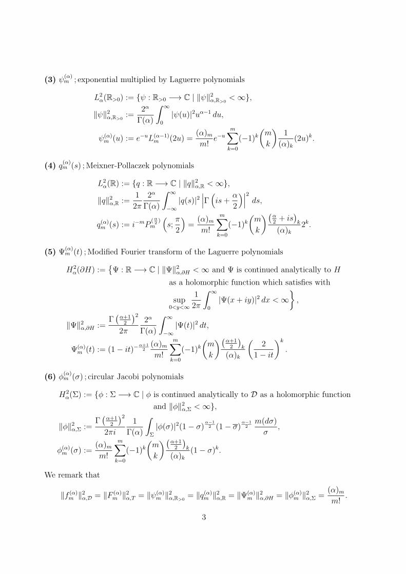
(3) ψ(α)m ; exponential multiplied by Laguerre polynomials

L2α(R>0) := ψ : R>0 −→ C | ∥ψ∥2α,R>0

<∞,

∥ψ∥2α,R>0:=

2α

Γ(α)

∫ ∞

0

|ψ(u)|2uα−1 du,

ψ(α)m (u) := e−uL(α−1)

m (2u) =(α)mm!

e−u

m∑k=0

(−1)k(m

k

)1

(α)k(2u)k.

(4) q(α)m (s) ;Meixner-Pollaczek polynomials

L2α(R) := q : R −→ C | ∥q∥2α,R <∞,

∥q∥2α,R :=1

2π

2α

Γ(α)

∫ ∞

−∞|q(s)|2

∣∣∣Γ(is+ α

2

)∣∣∣2 ds,q(α)m (s) := i−mP

(α2)

m

(s;π

2

)=

(α)mm!

m∑k=0

(−1)k(m

k

)(α2+ is

)k

(α)k2k.

(5) Ψ(α)m (t) ;Modified Fourier transform of the Laguerre polynomials

H2α(∂H) :=

Ψ : R −→ C | ∥Ψ∥2α,∂H <∞ and Ψ is continued analytically to H

as a holomorphic function which satisfies with

sup0<y<∞

1

2π

∫ ∞

0

|Ψ(x+ iy)|2 dx <∞,

∥Ψ∥2α,∂H :=Γ(α+12

)22π

2α

Γ(α)

∫ ∞

−∞|Ψ(t)|2 dt,

Ψ(α)m (t) := (1− it)−

α+12(α)mm!

m∑k=0

(−1)k(m

k

)(α+12

)k

(α)k

(2

1− it

)k

.

(6) ϕ(α)m (σ) ; circular Jacobi polynomials

H2α(Σ) := ϕ : Σ −→ C | ϕ is continued analytically to D as a holomorphic function

and ∥ϕ∥2α,Σ <∞,

∥ϕ∥2α,Σ :=Γ(α+12

)22πi

1

Γ(α)

∫Σ

|ϕ(σ)|2(1− σ)α−12 (1− σ)

α−12m(dσ)

σ,

ϕ(α)m (σ) :=

(α)mm!

m∑k=0

(−1)k(m

k

)(α+12

)k

(α)k(1− σ)k.

We remark that

∥f (α)m ∥2α,D = ∥F (α)

m ∥2α,T = ∥ψ(α)m ∥2α,R>0

= ∥q(α)m ∥2α,R = ∥Ψ(α)m ∥2α,∂H = ∥ϕ(α)

m ∥2α,Σ =(α)mm!

.

3

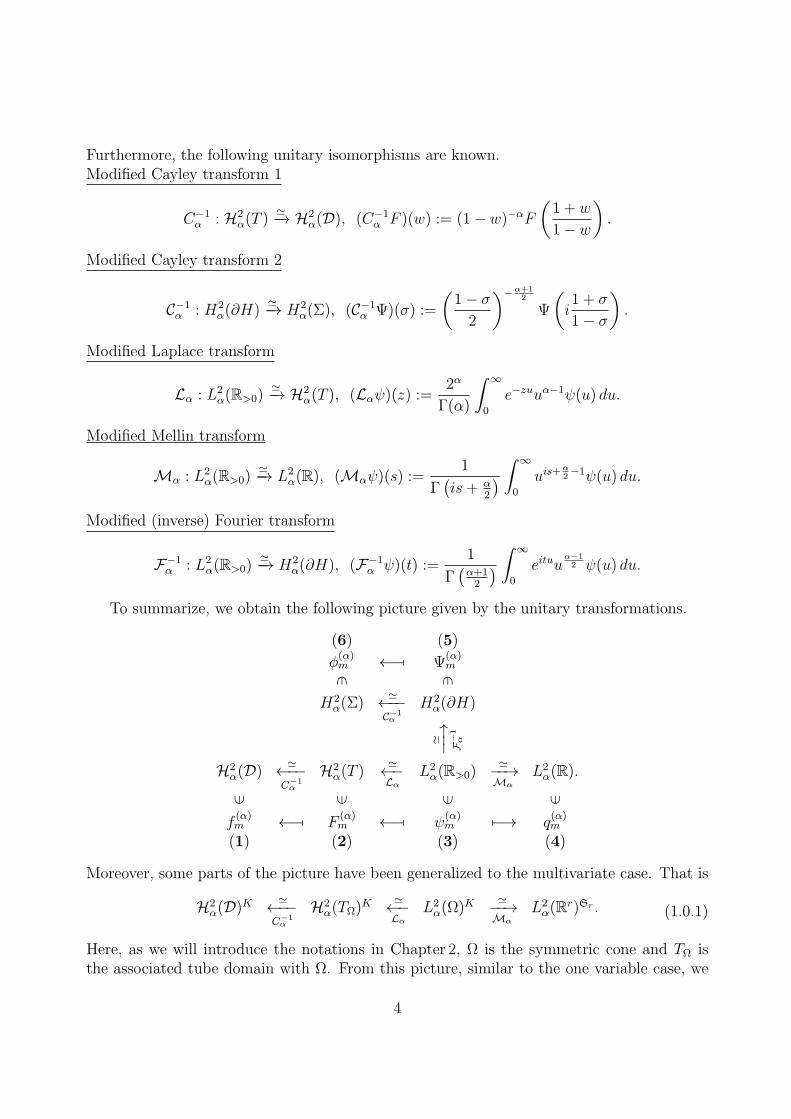
Furthermore, the following unitary isomorphisms are known.Modified Cayley transform 1

C−1α : H2

α(T )≃−→ H2

α(D), (C−1α F )(w) := (1− w)−αF

(1 + w

1− w

).

Modified Cayley transform 2

C−1α : H2

α(∂H)≃−→ H2

α(Σ), (C−1α Ψ)(σ) :=

(1− σ2

)−α+12

Ψ

(i1 + σ

1− σ

).

Modified Laplace transform

Lα : L2α(R>0)

≃−→ H2α(T ), (Lαψ)(z) :=

2α

Γ(α)

∫ ∞

0

e−zuuα−1ψ(u) du.

Modified Mellin transform

Mα : L2α(R>0)

≃−→ L2α(R), (Mαψ)(s) :=

1

Γ(is+ α

2

) ∫ ∞

0

uis+α2−1ψ(u) du.

Modified (inverse) Fourier transform

F−1α : L2

α(R>0)≃−→ H2

α(∂H), (F−1α ψ)(t) :=

1

Γ(α+12

) ∫ ∞

0

eituuα−12 ψ(u) du.

To summarize, we obtain the following picture given by the unitary transformations.

(6) (5)

ϕ(α)m ←− [ Ψ

(α)m

∋ ∋

H2α(Σ)

≃←−−C−1α

H2α(∂H)

≃ −−→

F−1

α

H2α(D)

≃←−−C−1

α

H2α(T )

≃←−Lα

L2α(R>0)

≃−−→Mα

L2α(R).

∈ ∈ ∈ ∈

f(α)m ←− [ F

(α)m ←− [ ψ

(α)m 7−→ q

(α)m

(1) (2) (3) (4)

Moreover, some parts of the picture have been generalized to the multivariate case. That is

H2α(D)K

≃←−−C−1

α

H2α(TΩ)

K ≃←−Lα

L2α(Ω)

K ≃−−→Mα

L2α(Rr)Sr . (1.0.1)

Here, as we will introduce the notations in Chapter 2, Ω is the symmetric cone and TΩ isthe associated tube domain with Ω. From this picture, similar to the one variable case, we

4

obtain the well-known correspondence between Laguerre and spherical polynomials. A linkbetween Laguerre and Meixner-Pollaczek polynomials from a spherical Fourier transform hasrecently been established that was also established by Davidson, Olafsson and Zhang [DOZ],and Faraut and Wakayama [FW1]. This setting is not only beneficial for introducing theabove orthogonal systems, but also studying their fundamental properties (orthogonality,generating functions, difference or differential equations and recurrence formulas).

This thesis has two purposes. The first is to study a multivariate analogue of the resultsobtained by Shen [She]. Namely, we consider a modified Fourier transform of L2

α(Ω)K and

multivariate Laguerre polynomials. Using this unitary isomorphism and the modified Cayleytransform, we introduce some new multivariate special orthogonal polynomials, which area multivariate analogue of circular Jacobi polynomials. These polynomials, which we callmultivariate circular Jacobi (MCJ) polynomials, are generalizations of the spherical (zonal)polynomials that are different from the Jack or Macdonald polynomials, which are wellknown as an extension of spherical polynomials. We also remark that the weight functionof their orthogonality relation coincides with the circular Jacobi ensemble defined by Bour-gade et al. [BNR]. Furthermore, we provide a generating function for the MCJ polynomialsand a differential equation that is satisfied by the modified Cayley transform of the MCJpolynomials.

The second purpose is to introduce some multivariate discrete orthogonal polynomi-als within the setting (1.0.1) that are multivariate analogues of Meixner, Charlier andKrawtchouk polynomials, and to establish their main properties, that is, duality, degener-ate limits, generating functions, orthogonality relations, difference equations and recurrenceformulas. A particularly important and interesting result is that “the generating function ofthe generating function” for the Meixner polynomials coincides with the generating functionof the Laguerre polynomials. We derive the above properties for the multivariate Meixner,Charlier and Krawtchouk polynomials from some properties of the multivariate Laguerrepolynomials and the unitary picture (1.0.1) by using this key lemma. This scheme has pre-viously not been known even for the one variable case. It is also interesting to note that thereis correspondence between Laguerre and Meixner polynomials. The former has orthogonalitydefined by the integral on the symmetric cone and the latter is defined by the summationon partitions.

Let us now describe the content of the following chapters. The basic definitions andfundamental properties of Jordan algebras and symmetric cones, and lemmas for analysis onsymmetric cones and tube domains have been presented in the first section of Chapter 2, sothat they can be referred to later. The next section presents a compilation of basic facts forthe multivariate Laguerre polynomials and their unitary picture. In particular, we constructthe unitary isomorphism between L2

α(Ω)K and L2

α,θ(Rr)Sr . Since we do not need to use theGutzmer formula, our construction is much simpler than [FW1] and is regarded as a multipleanalogue of Koornwinder’s construction [Ko]. Based on these preparations, in Chapter 3, we

5

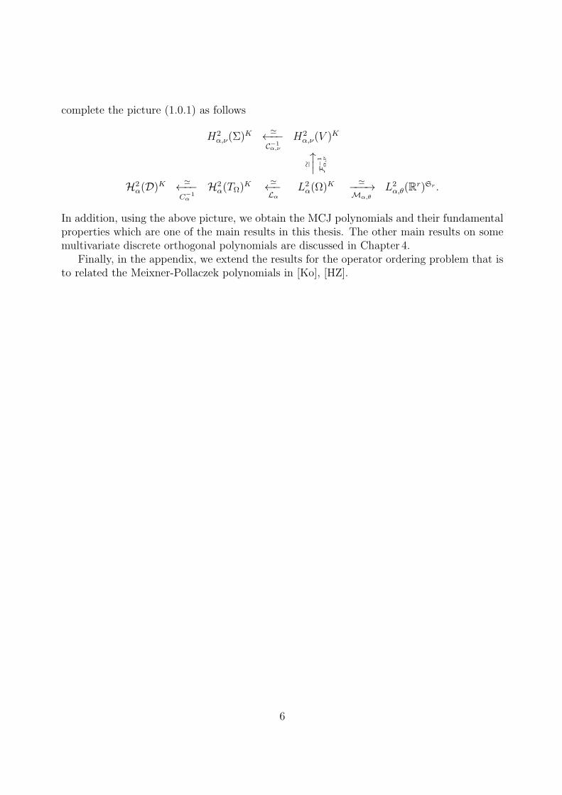
complete the picture (1.0.1) as follows

H2α,ν(Σ)

K ≃←−−C−1α,ν

H2α,ν(V )K

≃ −−→

F−1

α,ν

H2α(D)K

≃←−−C−1

α

H2α(TΩ)

K ≃←−Lα

L2α(Ω)

K ≃−−−→Mα,θ

L2α,θ(Rr)Sr .

In addition, using the above picture, we obtain the MCJ polynomials and their fundamentalproperties which are one of the main results in this thesis. The other main results on somemultivariate discrete orthogonal polynomials are discussed in Chapter 4.

Finally, in the appendix, we extend the results for the operator ordering problem that isto related the Meixner-Pollaczek polynomials in [Ko], [HZ].

6

Acknowledgements

First and foremost, I would like to express my sincere gratitude to Professor MasatoWakayama.He guided me toward studying multivariate special orthogonal polynomial systems, which isthe main theme in this thesis and gave me much useful advice as my supervisor.

I would also like to express my deep gratitude to the examiners, Professor Hiroyuki Ociai,Toshio Oshima and Toru Umeda.

In addition, I would like to thank the people who helped me and advised me on manyissues in my thesis. Especially, I would like to express my sincere gratitude to ProfessorHiroyuki Ochiai who gave me a chance to talk about my thesis in his laboratory and varioususeful advice, not only about mathematics, but about my academic life. I am also grateful toProfessor Takaaki Nomura for his helpful advice and information for analysis on symmetriccones, and Professor Katsuhiko Kikuchi for his valuable suggestions on the shifted Schurand Jack polynomials. I am also indebted to Professor Saburo Kakei for the productive dis-cussions on multivariate special orthogonal polynomials and degenerate double affine Heckealgebra and to Professor Satoshi Tsujimoto and Hiroshi Miki for the beneficial information onthe multivariate discrete orthogonal polynomials, and to Professor Tomoyuki Shirai for thevaluable advice for random matrix theory. I also wish to thank Professor Masatoshi Noumi,Toshio Oshima and Toru Umeda for the constructive advice they provided on representationtheory, harmonic analysis, quantum integral systems and some special functions.

Further, I am greatly indebted to the Faculty of Mathematics of Kyushu University,particularly, the office staff and the staff of research room 4.

My academic career would have been impossible without generous funding by the GlobalCOE Program of the ”Education-and-Research Hub for Mathematics-for-Industry” of theGraduate School of Mathematics at Kyushu University and a Grant-in-Aid for JSPS Fellowsfrom April 2012 to March 2014, which supported various research activities.

My special thanks go to the Kawamura family in Kyoto, and Mr. Takafumi Aizawa andMrs. Sayaka Aizawa who supported me in attending seminars, workshops and conferencesin Kyoto or Tokyo.

Finally, I would like to give my exceptional thanks to my mother Takako Shibukawa,my grandfather Shinichi Tsuboi, my grandmother Norie Tsuboi, my uncle Haruhiko Tsuboiand my aunt Mayumi Tsuboi for their longtime support. Further, I would also like toposthumously thank my father Hiroki Shibukawa who passed away twenty six years agoat the young age of twenty-eight, and my great-grandfather Itsuji Tsuboi and my great-grandmother Fumiyo Tsuboi who have also passed away.

7

Chapter 2

Preliminaries

Throughout the paper, we denote the ring of rational integers by Z, the field of real numbersby R, the field of complex numbers by C, the partition set of length r by P

P := m = (m1, . . . ,mr) ∈ Zr≥0 | m1 ≥ · · · ≥ mr. (2.0.1)

For any vector s = (s1, . . . , sr) ∈ Cr, we put

Re s := (Re s1, . . . ,Re sr), (2.0.2)

|s| := s1 + · · ·+ sr, (2.0.3)

∥s∥ := (|s1|, . . . , |sr|). (2.0.4)

Moreover, for m ∈Pm! := m1! · · ·mr!

and we set δ := (r − 1, r − 2, . . . , 1, 0). Refer to Faraut and Koranyi [FK] for the details inthis chapter.

2.1 Analysis on symmetric cones

Let Ω be an irreducible symmetric cone in V which is a finite dimensional simple EuclideanJordan algebra of dimension n as a real vector space and rank r. The classification of irre-ducible symmetric cones is well-known. Namely, there are four families of classical irreduciblesymmetric cones Πr(R),Πr(C),Πr(H), the cones of all r × r positive definite matrices overR, C and H, the Lorentz cones Λr and an exceptional cone Π3(O) (see [FK] p. 97). Also, letV C be its complexification. For w, z ∈ V C, we define

L(w)z := wz,

wz := L(wz) + [L(w), L(z)],

P (w, z) := L(w)L(z) + L(z)L(w)− L(wz),P (w) := P (w,w) = 2L(w)2 − L(w2).

8

We denote the Jordan trace and determinant of the complex Jordan algebra V C by tr x andby ∆(x) respectively.

Fix a Jordan frame c1, . . . , cr that is a complete system of orthogonal primitive idem-potents in V and define the following subspaces:

Vj := x ∈ V | L(cj)x = x,

Vjk :=

x ∈ V

∣∣∣∣L(cj)x =1

2x and L(ck)x =

1

2x

.

Then, Vj = Rej for j = 1, . . . , r are 1-dimensional subalgebras of V , while the subspaces Vjkfor j, k = 1, . . . , r with j < k all have a common dimension d = dimR Vjk. Then, V has thePeirce decomposition

V =

(r⊕

j=1

Vj

)⊕

(⊕j<k

Vjk

),

which is the orthogonal direct sum. It follows that n = r + d2r(r − 1). Let G(Ω) denote

the automorphism group of Ω and let G be the identity component in G(Ω). Then, G actstransitively on Ω and Ω ∼= G/K where K ∈ G is the isotropy subgroup of the unit element,e ∈ V . K is also the identity component in Aut (V ).

For any x ∈ V , there exists k ∈ K and λ1, . . . , λr ∈ R such that

x = kr∑

j=1

λjcj, (λ1 ≥ · · · ≥ λr).

From this polar decomposition, we obtain the following integral formula (see [FK]TheoremVI. 2.3).

Lemma 2.1.1. Let f be an integrable function on V. We have∫V

f(x) dx = c0

∫K×Rr

f(kλ)∏

1≤p<q≤r

|λp − λq|d dkdλ1 · · · dλr. (2.1.1)

Here, dx is the Euclidean measure associated with the Euclidean structure on V given by(u|v) = tr(uv), dk is the normalized Haar measure on the compact group K, λ =

∑rj=1 λjcj

and c0 is defined by

c0 := (2π)n−r2

r∏j=1

Γ(d2+ 1)

Γ(d2j + 1

) =(2π)

n−r2

r!

r∏j=1

Γ(d2

)Γ(d2j) . (2.1.2)

In particular, for f ∈ L1(V )K∫V

f(x) dx = c0

∫Rr

f(λ1, . . . , λr)∏

1≤p<q≤r

|λp − λq|d dλ1 · · · dλr. (2.1.3)

9

As in the case of V , we also have the following spectral decomposition for V C. Every zin V C can be written

z = ur∑

j=1

λjcj,

with u in U which is the identity component of Str(V C) ∩ U(V C), λ1 ≥ · · · ≥ λr ≥ 0.Moreover, we define the spectral norm of z ∈ V C by |z| = λ1 and introduce open unit ballD ∈ V C as follows.

D = z ∈ V C | |z| < 1.

We define Σ as the set of invertible elements in V C such that z−1 = z, which coin-cides with the Shilov boundary of D. For Σ, the following result is well known (see [FK]PropositionX.2.3).

Lemma 2.1.2. For z ∈ V C, the following properties are equivalent:(i) z ∈ Σ,(ii) z = eiθ =

∑rj=1 e

iθjcj with θ =∑r

j=1 θjcj ∈ V ,

(iii) z ∈ c−1(V ),where c−1(t) := (t− ie)(t+ ie)−1 = e− 2i(t+ ie)−1 is called the inverse Cayley transform.

We will later need the following integral formula on Σ to describe the MCJ polynomials.

Lemma 2.1.3. Let µ denote the measure associated with the Riemannian structure on Σinduced by the Euclidean structure of V C.(1) If ϕ is an integrable function on Σ, then∫

Σ

ϕ(σ) dµ(σ) = 2n∫V

ϕ(c−1(t))|∆(e− it)−nr |2 dt. (2.1.4)

(2) If Ψ is an integrable function on V , then∫V

Ψ(t) dt = 2n∫Σ

Ψ(c(σ))|∆(e− σ)−nr |2 dµ(σ). (2.1.5)

Here, c is a Cayley transform defined by c(σ) := i(e+ σ)(e− σ)−1 = −ie+ 2i(e− σ)−1.(3) If Ψ is an integrable function on V and a K-invariant, then∫

Σ

ϕ(σ) dµ(σ) = c0

∫Sr

ϕ(eiθ)∏

1≤p<q≤r

|eiθp − eiθq |d dθ1 · · · dθr. (2.1.6)

Here, Sr is the direct product of r copies of S1.

Proof. (1) is PropositionX.2.4 of [FK] itself and (2) also immediately follows from someproposition. Hence, we only prove (3).

Let ϕ ∈ L1(Σ)K . Since for any k ∈ K

c−1(kt) = (k(t− ie))(k(t+ ie))−1 = k((t+ ie)(t− ie)−1) = kc−1(t),

10

from Lemma2.1.1, we have∫Σ

ϕ(σ) dµ(σ) = 2n∫V

ϕ(c−1(t))∆(e+ t2)−nr dt

= 2nc0

∫K×Rr

ϕ(c−1(kλ))∆(e+ (kt)2)−nr

∏1≤p<q≤r

|λp − λq|d dkdλ1 · · · dλr

= 2nc0

∫Rr

ϕ(c−1(λ))∆(e+ λ2)−nr

∏1≤p<q≤r

|λp − λq|d dλ1 · · · dλr.

If we put λj = − cot(

θj2

), then

λ = −r∑

j=1

cot

(θj2

)cj = i

r∑j=1

1 + eiθj

1− eiθjcj = i

(r∑

j=1

(1 + eiθj)cj

)(r∑

l=1

(1− eiθl)cl

)−1

= c(eiθ).

Therefore,

∫Σ

ϕ(σ) dµ(σ) = 2n−rc0

∫Sr

ϕ(eiθ)r∏

j=1

sin

(θj2

)2(nr−1)∏1≤p<q≤r

∣∣∣∣∣∣ sin(12(θp − θq)

)sin(

θp2

)sin(

θq2

)∣∣∣∣∣∣d

dθ1 · · · dθr

= c0

∫Sr

ϕ(eiθ)∏

1≤p<q≤r

|eiθp − eiθq |d dθ1 · · · dθr.

For j = 1, . . . , r, let ej := c1 + · · ·+ cj, and set

V (j) := x ∈ V | L(ej)x = x.

Denote the orthogonal projection of V onto the subalgebra V (j) by Pj, and define

∆j(x) := δj(Pjx)

for x ∈ V , where δj denotes the Koecher norm function for V (j). In particular, δr = ∆.Then, ∆j is a polynomial on V that is homogeneous of degree j. Let s := (s1, . . . , sr) ∈ Cr

and define the function ∆s on V by

∆s(x) := ∆(x)srr−1∏j=1

∆j(x)sj−sj+1 . (2.1.7)

That is the generalized power function on V . Furthermore, for m ∈ P, ∆m becomes apolynomial function on V , which is homogeneous of degree |m|.

11

The gamma function ΓΩ for the symmetric cone Ω is defined, for s ∈ Cr, with Re sj >d2(j − 1) (j = 1, . . . , r) by

ΓΩ(s) :=

∫Ω

e−tr(x)∆s(x)∆(x)−nr dx. (2.1.8)

Its evaluation gives

ΓΩ(s) = (2π)n−r2

r∏j=1

Γ

(sj −

d

2(j − 1)

). (2.1.9)

Hence, ΓΩ extends analytically as a meromorphic function on Cr.

Lemma 2.1.4. For any y ∈ Ω, β ∈ C,Re β > 0 and Re sj >d2(j − 1) :∫

Ω

e−(βy|x)∆s(x)∆(x)−nr dx = ΓΩ(s)∆s((βy)

−1). (2.1.10)

For s ∈ Cr and m ∈P, we define the generalized shifted factorial by

(s)m :=ΓΩ(s+m)

ΓΩ(s). (2.1.11)

It follows from (2.1.9) that

(s)m =r∏

j=1

(sj −

d

2(j − 1)

)mj

. (2.1.12)

Lemma 2.1.5. If s ∈ Cr,m,k ∈P and m ⊃ k, then∣∣∣∣(s)m(s)k

∣∣∣∣ ≤ (∥s∥+ d(r − 1))m(∥s∥+ d(r − 1))k

. (2.1.13)

Proof. We remark that for any s ∈ C, N ∈ Z≥0 and j = 1, . . . , r, the following is satisfied.∣∣∣∣s+N − d

2(j − 1)

∣∣∣∣ ≤ |s|+N + d(r − 1)− d

2(j − 1) = |s|+N +

d

2(2r − j − 1).

Hence, ∣∣∣∣(s)m(s)k

∣∣∣∣ = r∏j=1

∣∣∣∣∣(sj + kj −

d

2(j − 1)

)mj−kj

∣∣∣∣∣≤

r∏j=1

(|sj|+ kj + d(r − 1)− d

2(j − 1)

)mj−kj

=(∥s∥+ d(r − 1))m(∥s∥+ d(r − 1))k

.

12

Corollary 2.1.6. If s ∈ Cr,m ∈P, then

|(s)m| ≤ (∥s∥+ d(r − 1))m ≤r∏

j=1

(|sj|+ d(r − 1))mj. (2.1.14)

The space, P(V ), of the polynomial ring on V has the following decomposition.

P(V ) =⊕m∈P

Pm,

where each Pm are mutually inequivalent, and finite dimensional irreducible G-modules.Further, their dimensions are denoted by dm. For dm, the following formula is known (see,[Up] Lemma 2.6 or [FK] p. 315).

Lemma 2.1.7. For any m ∈P,

dm =c(−ρ)

c(ρ−m)c(m− ρ)(2.1.15)

=∏

1≤p<q≤r

mp −mq +d2(q − p)

d2(q − p)

B(mp −mq,

d2(q − p− 1) + 1

)B(mp −mq,

d2(q − p+ 1)

) (2.1.16)

=Γ(d2

)rΓ(d2r) r−1∏

j=1

1

Γ(d2j)2 ∏

1≤p<q≤r

(mp −mq +d

2(q − p))

Γ(mp −mq +

d2(q − p+ 1)

)Γ(mp −mq +

d2(q − p− 1) + 1

) .(2.1.17)

Here, ρ = (ρ1, . . . , ρr), ρj :=d4(2j − r − 1), and c is the Harish-Chandra function:

c(s) =∏

1≤p<q≤r

B(sq − sp, d2

)B(d2(q − p), d

2

) .In particular, for d = 2

dm =∏

1≤p<q≤r

(mp −mq + q − p

q − p

)2

= sm(1, . . . , 1)2. (2.1.18)

Here, sm is the Schur polynomial corresponding to m ∈P defined by

sm(λ1, . . . , λr) :=det (λmk+r−k

j )

det (λr−kj )

.

The following lemma is necessary to evaluate the Fourier transform of the multivariateLaguerre polynomial.

13

Lemma 2.1.8 ([FK]TheoremXI. 2.3). For p ∈ Pm, Reα > (r − 1)d2, and y ∈ Ω + iV ,∫

Ω

e−(y|x)p(x)∆(x)α−nr dx = ΓΩ(m+ α)∆(y)−αp(y−1). (2.1.19)

Here, α is regarded as (α, . . . , α) ∈ Cr.

For each m ∈P, the spherical polynomial of weight |m| on Ω is defined by

Φ(d)m (x) :=

∫K

∆m(kx) dk. (2.1.20)

We often omit multiplicity d of Φ(d)m (x). The algebra of all K-invariant polynomials on V ,

denoted by P(V )K , decomposes as

P(V )K =⊕m∈P

CΦm.

By analytic continuation to the complexification V C of V , we can extend tr ,∆ and Φm topolynomial functions on V C.

Remark 2.1.9. (1) Since Φm ∈ PKm , for x = k

∑rj=1 λjcj, Φm(x) can be expressed by

Φm(λ1, . . . , λr) := Φm

(r∑

j=1

λjcj

)(= Φm(x)).

Φm(x) also has the following expression (see [F]).

Φ(d)k (λ1, . . . , λr) =

P( 2d)

k (λ1, . . . , λr)

P( 2d)

k (1, . . . , 1). (2.1.21)

Here, P( 2d)

k (λ1, . . . , λr) is an r-variable Jack polynomial (see [M], Chapter. VI.10). In partic-

ular, since P(1)k (λ1, . . . , λr) = sm(λ1, . . . , λr), Φ

(2)m becomes the Schur polynomial.

Φ(2)m (λ1, . . . , λr) =

sm(λ1, . . . , λr)

sm(1, . . . , 1)=

δ!∏p<q(mp −mq + q − p)

sm(λ1, . . . , λr). (2.1.22)

(2)When r = 2, Φ(d)m has the following hypergeometric expression (see [Sa]).

Φ(d)m1,m2

(λ1, λ2) = λm11 λm2

2 2F1

(−(m1 −m2),

d2

d;λ1 − λ2λ1

)= λm1

1 λm22

(d2

)m1−m2

(d)m1−m2

2F1

(−(m1 −m2),

d2

−(m1 −m2)− d2+ 1

;λ2λ1

).

14

We remark that the function Φm(e + x) is a K-invariant polynomial of degree |m| anddefine the generalized binomial coefficients

(mk

)d2

by using the following expansion.

Φ(d)m (e+ x) =

∑|k|≤|m|

(m

k

)d2

Φ(d)k (x). (2.1.23)

For(mk

)d2

, we also often omit d2. The fact that if k ⊂m, then

(mk

)= 0, is well known. Hence,

we have

Φm(e+ x) =∑k⊂m

(m

k

)Φk(x). (2.1.24)

Lemma 2.1.10. For z = u∑r

j=1 λjcj with u ∈ U , λ1 ≥ · · · ≥ λr ≥ 0 and m ∈P, we have

|Φm(z)| ≤ λm11 · · ·λmr

r ≤ λ|m|1 = Φm(λ1). (2.1.25)

Lemma 2.1.11. For any α ∈ C, z ∈ D, w ∈ D, we have∑m∈P

dm(α)m(nr

)m

Φm(z)Φm(w) = ∆(w)−α

∫K

∆(kw−1 − z)−α dk. (2.1.26)

The spherical function, φs, on Ω for s ∈ Cr is defined by

φs(x) :=

∫K

∆s+ρ(kx) dk. (2.1.27)

We remark that for x ∈ Ωφs(x

−1) = φ−s(x) (2.1.28)

and for x ∈ Ω,m ∈PΦm(x) = φm−ρ(x). (2.1.29)

Let D(Ω) be the algebra of G-invariant differential operators on Ω, P(V )K be the spaceof K-invariant polynomials on V , and P(V × V )G be the space of polynomials on V × V ,which are invariant in the sense that

p(gx, ξ) = p(x, g∗ξ), (g ∈ G).

Here, we write g∗ for the adjoint of an element g (i.e., (gx|y) = (x|g∗y) for all x, y ∈ V ). Thespherical function φs is an eigenfunction of every D ∈ D(Ω). Thus, we denote its eigenvaluesby γ(D)(s), that is, Dφs = γ(D)(s)φs.

The symbol σD of a partial differential operator D which acts on the variable x ∈ V isdefined by

De(x|ξ) = σD(x, ξ)e(x|ξ) (x, ξ ∈ V ).

Differential operator D on Ω is invariant under G if and only if its symbol σD belongs toP(V ×V )G. In addition, the map D 7→ σD establishes a linear isomorphism from D(Ω) onto

15

P(V × V )G. Moreover, the map D 7→ σD(e, u) is a vector space isomorphism from D(Ω)onto P(V )K . In particular, for k ∈P, s ∈ Cr, we put

γk(s) := γ(Φk(∂x))(s) = Φk(∂x)φs(x)|x=e. (2.1.30)

Here, Φk(∂x) is a unique G-invariant differential operator, which is satisfied with

σΦk(∂x)(e, ξ) = Φk(ξ) ∈ P(V )K , i.e., Φk(∂x)e(x|ξ)|x=e = Φk(ξ)e

tr ξ.

We remark that Φk(∂x) = ∂kx and γk(s) = s(s− 1) · · · (s− k + 1) in the r = 1 case, and forany α ∈ C, k ∈P, we have

γk(α− ρ) = (−1)|k|(−α)k. (2.1.31)

The function γD is an r variable symmetric polynomial and map D 7→ γD is an algebraisomorphism from D(Ω) onto algebra P(Rr)Sr , which is a special case of the Harish-Chandraisomorphism.

Lemma 2.1.12. If β ∈ C,Re β > 0,Re sj >d4(r − 1), then for all k ∈P, we have∫

Ω

e−β tr uΦk(u)φs(u)∆(u)−nr du = (−1)|k|β−|s+k|ΓΩ(s+ ρ)γk(−s). (2.1.32)

Here, we choose the branch of β−|s|, which takes the value 1 at β = 1.

Proof. We remark that the left hand side of (2.1.32) is converges absolutely under the as-sumptions. Hence,∫

Ω

e−β tr uΦk(u)φs(u)∆(u)−nr du = (−β)−|k|

∫Ω

Φk(∂x)e−(βx|u)|x=eφs(u)∆(u)−

nr du

= (−β)−|k|Φk(∂x)

∫Ω

∫K

e−(βx|u)∆s+ρ(ku)∆(u)−nr dkdu

∣∣∣∣x=e

= (−β)−|k|Φk(∂x)

∫K

∫Ω

e−(βkx|u)∆s+ρ(u)∆(u)−nr dudk

∣∣∣∣x=e

.

By Lemma2.1.4,∫Ω

e−(βkx|u)∆s+ρ(u)∆(u)−nr du = ΓΩ(s+ ρ)∆s+ρ((βkx)

−1) = β−|s|ΓΩ(s+ ρ)∆s+ρ((kx)−1).

Therefore,∫Ω

e−β tr uΦk(u)φs(u)∆(u)−nr du = (−1)|k|β−|s+k|ΓΩ(s+ ρ)Φk(∂x)

∫K

∆s+ρ(kx−1) dk

∣∣∣∣x=e

= (−1)|k|β−|s+k|ΓΩ(s+ ρ)Φk(∂x)φ−s(x)|x=e.

16

If a K-invariant function ψ is analytic in the neighborhood of e, it admits a sphericalTaylor expansion near e:

ψ(e+ x) =∑k∈P

dk1(nr

)k

Φk(∂x)ψ(x)|x=eΦk(x).

By the definition of γk, we have

φs(e+ x) =∑k∈P

dk1(nr

)k

γk(s)Φk(x).

Since Φm = φm−ρ, (m

k

)= dk

1(nr

)k

γk(m− ρ).

For a complex number α, we define the following differential operator on Ω:

Dα = ∆(x)1+α∆(∂x)∆(x)−α.

For this operator, we have

γ(Dα)(s) =r∏

j=1

(sj − α+

d

4(r − 1)

). (2.1.33)

The operators Dj d2, j = 0, . . . , r − 1 generate algebra D(Ω).

Lemma 2.1.13. For all k ∈ P, there exist some constant C > 0 and integer N such thatfor any s ∈ Cr

|γk(s)| ≤ C

r∏l=1

(|sl|+

d

4(r − 1)

)N

. (2.1.34)

|γk(s− ρ)| ≤ C

r∏l=1

(|sl|+

d

2(r − 1)

)N

. (2.1.35)

Proof. Since algebra D(Ω) is generated by Dj d2, j = 0, . . . , r − 1, for Φk(∂x) ∈ D(Ω),

Φk(∂x) =∑

l0,...,lr−1;finite

al0,...,lr−1Dl00 d2

· · ·Dlr−1

(r−1) d2

.

Here, we remark that for j = 0, . . . , r − 1

|γ(D d2(j−1))(s)| =

∣∣∣∣∣r∏

l=1

(sl +

d

4(r − 1)− d

2(j − 1)

)∣∣∣∣∣ ≤r∏

l=1

(|sl|+

d

4(r − 1)

).

Therefore,

|γk(s)| ≤∑

l0,...,lr−1;finite

|al0,...,lr−1 |γ(D0 d2)(s)l0 · · · γ(D(r−1) d

2)(s)lr−1 ≤ C

r∏l=1

(|sl|+

d

4(r − 1)

)N

.

We immediately derive (2.1.35) from (2.1.34).

17

Lemma 2.1.14. For all s ∈ Cr, there exist some l ∈ Z≥0 and some constant C > 0 suchthat for all l ⊂ k ∈P

|γk(−s)| ≤ CΓΩ(Re (s) + ρ+ k)

|ΓΩ(s)|≤ C

∣∣∣∣ΓΩ(Re (s) + ρ)

ΓΩ(s)

∣∣∣∣ (∥Re (s)∥+ d(r − 1))k. (2.1.36)

Proof. For fixed s ∈ Cr, we assume the integral∫Ω

|e− tr uΦl(u)∆s+ρ(u)∆(u)−nr | du

converges absolutely. Hence, for all l ⊂ k ∈P,∫Ω

|e− tr uΦk(u)∆s+ρ(u)∆(u)−nr | du <∞.

By Lemma2.1.12,

γk(−s) =(−1)|k|

ΓΩ(s)

∫Ω

e− tr uΦk(u)∆s+ρ(u)∆(u)−nr du.

Hence,

|γk(−s)| ≤1

|ΓΩ(s)|

∫Ω

e− tr uΦk(u)|∆s+ρ(u)|∆(u)−nr du

≤ 1

|ΓΩ(s)|

∫K

∫Ω

e− tr u∆k(u)∆Re (s)+ρ(ku)∆(u)−nr dudk.

Since K is a compact group and∫Kdk = 1, there exists some k ∈ K such that∫

K

∫Ω

e− tr u∆k(u)∆Re (s)+ρ(ku)∆(u)−nr dudk ≤

∫Ω

e− tr u∆k(u)∆Re (s)+ρ(ku)∆(u)−nr du.

Moreover, since ∆k is a homogeneous degree |k| polynomial and k ∈ K is a linear transfor-mation on V , there exists some constant C > 0 such that∫

Ω

e− tr u∆k(ku)∆Re (s)+ρ(u)∆(u)−nr du ≤ C

∫Ω

e− tr u∆Re (s)+ρ+k(u)∆(u)−nr du.

Therefore, by using the definition of ΓΩ, we have

|γk(−s)| ≤C

|ΓΩ(s)|

∫Ω

e− tr u∆Re (s)+ρ+k(u)∆(u)−nr du

= CΓΩ(Re (s) + ρ+ k)

|ΓΩ(s)|

≤ C

∣∣∣∣ΓΩ(Re (s) + ρ)

ΓΩ(s)

∣∣∣∣ |(Re (s) + ρ)k|

≤ C

∣∣∣∣ΓΩ(Re (s) + ρ)

ΓΩ(s)

∣∣∣∣ (∥Re (s)∥+ d(r − 1))k.

18

The final inequality follows from

|(Re (s) + ρ)k| =r∏

j=1

∣∣∣∣∣(Re (s) + ρj −

d

2(j − 1)

)kj

∣∣∣∣∣≤

r∏j=1

(|Re (s)|+ d

2(r − 1)

)kj

≤ (∥Re (s)∥+ d(r − 1))k.

Lemma 2.1.15. For all m,k ∈P, we have

γk(m− ρ) ≥ 0. (2.1.37)

Proof. Since γk(m − ρ) = 1dk

(nr

)k

(mk

)and dk,

(nr

)k> 0, it suffices to show

(mk

)≥ 0 for all

m,k ∈P. From [OO], generalized binomial coefficients are written as(m

k

)d2

=P ∗k

(m; d

2

)H( d

2)(k)

,

where P ∗k

(m; d

2

)is the shifted Jack polynomial and H( d

2)(k) > 0 is a deformation of the hook

length. Moreover, by using (5.2) in [OO]

P ∗k

(m;

d

2

)=

d2- dimm/kd2- dimm

|m|(|m| − 1) · · · (|m| − |k|+ 1).

Further, the positivity of the generalized dimensions of the skew Young diagram, d2- dimm/k,

follows from (5.1) of [OO] and Chapter VI. 6 of [M]. Therefore, we obtain the positivity ofthe shifted Jack polynomial and the conclusion.

Theorem 2.1.16. (1) For w ∈ D,k ∈P, α ∈ C, we have

(α)k∆(e− w)−αΦk(w(e− w)−1) =∑x∈P

dx(α)x(nr

)x

γk(x− ρ)Φx(w). (2.1.38)

Here, we choose the branch of ∆(e− w)−α which takes the value 1 at w = 0.(2)For w ∈ V C,k ∈P, a K-invariant analytic function etr wΦk(w) has the following expan-sion.

etr wΦk(w) =∑x∈P

dx1(nr

)x

γk(x− ρ)Φx(w). (2.1.39)

Proof. (1)We take w = u∑r

j=1 λjcj ∈ D with u ∈ U and 1 > λ1 ≥ . . . ≥ λr ≥ 0. ByLemmas 2.1.10 and 2.1.13, there exist some C > 0 and N ∈ Z≥0 such that∑

x∈P

∣∣∣∣∣dx (α)x(nr

)x

γk(x− ρ)Φx(w)

∣∣∣∣∣ ≤∑x∈P

dx|(α)x|(

nr

)x

|γk(x− ρ)||Φx(w)|

≤ C

r∏l=1

∑xl≥0

(|α|+ d(r − 1))xl

xl!

(xl +

d

2(r − 1)

)N

λxll <∞.

19

Therefore, the right hand side of (2.1.38) converges absolutely. By analytic continuation, itis sufficient to show the assertion when Reα > d

2(r − 1) and w ∈ Ω ∩ (e− Ω) ⊂ D.

Φk(∂z)∑x∈P

dx(α)x(nr

)x

Φx(z)Φx(w)

∣∣∣∣z=e

=∑x∈P

dx(α)x(nr

)x

Φk(∂z)Φx(z)|z=eΦx(w)

=∑x∈P

dx(α)x(nr

)x

γk(x− ρ)Φx(w).

On the other hand,

Φk(∂z)∑x∈P

dx(α)x(nr

)x

Φx(z)Φx(w)

∣∣∣∣z=e

= Φk(∂z)∆(w)−α

∫K

∆(kw−1 − z)−α dk

∣∣∣∣z=e

= ∆(w)−α

∫K

Φk(∂z)∆(kw−1 − z)−α∣∣z=e

dk.

Here, from kw−1 − z ∈ TΩ for all k ∈ K and Lemma2.1.8,

Φk(∂z)∆(kw−1 − z)−α∣∣z=e

= Φk(∂z)1

ΓΩ(α)

∫Ω

e−(x|kw−1−z)∆(x)α∆(x)−nr dx

∣∣∣∣z=e

=1

ΓΩ(α)

∫Ω

Φk(∂z)e(x|z)|z=ee

−(x|kw−1)∆(x)α∆(x)−nr dx

=1

ΓΩ(α)

∫Ω

Φk(x)e−(kx|(w−1−e))∆(x)α∆(x)−

nr dx

= (α)k∆(w−1 − e)−αΦk((w−1 − e)−1).

Therefore,

Φk(∂z)∑x∈P

dx(α)x(nr

)x

Φx(z)Φx(w)

∣∣∣∣z=e

= ∆(w)−α

∫K

(α)k∆(w−1 − e)−αΦk((w−1 − e)−1) dk

= (α)k∆(e− w)−αΦk(w(e− w)−1).

(2) Since the right hand side of (2.1.39) converges absolutely due to a similar argument of(1), we have

etr wΦk(w) = limα→∞

(α)k∆(e− w

α

)−α

Φk

(w

α

(e− w

α

)−1)

=∑x∈P

dx1(nr

)x

γk(x− ρ) limα→∞

(α)xΦx

(wα

)=∑x∈P

dx1(nr

)x

γk(x− ρ)Φx(w).

20

Next, we preview the gradient for a C-valued and V -valued function f on simple EuclideanJordan algebra V . In this parts, we refer to [Di]. For differentiable function f : V → R andx, u ∈ V , we define the gradient, ∇f(x) ∈ V , of f by

(∇f(x)|u) = Duf(x) =d

dtf(x+ tu)

∣∣∣∣t=0

.

For a C-valued function f = f1 + if2, we define ∇f = ∇f1 + i∇f2. For z = x + iy ∈ V C,we define Dz = Dx + iDy. Moreover, if e1, . . . , en is an orthonormal basis of V andx =

∑nj=1 xjej ∈ V C, then

∇f(x) =n∑

j=1

∂f(x)

∂xjej.

We remark that this expression is independent of the choice of an orthonormal basis of V .For a V -valued function f : V → V expressed by f(x) =

∑rj=1 fj(x)ej, we define ∇f by

∇f(x) =n∑

j,l=1

∂fj(x)

∂xlejel.

That is also well defined. Let us present some derivation formulas.

Lemma 2.1.17. (1)The product rule of differentiation: For V -valued function f, h, we have

tr (∇(f(x)h(x))) = tr (∇f(x))h(x) + f(x) tr (∇h(x)). (2.1.40)

For C-valued functions f, h,

∇(f(x)h(x)) = (∇f(x))h(x) + f(x)(∇h(x)). (2.1.41)

(2)

∇x =n

re. (2.1.42)

(3)For any invertible element x ∈ V C,

tr (x∇)x−1 := tr (x(∇x−1)) = −nrtr x−1. (2.1.43)

(4)For β ∈ C and an invertible element x ∈ V C,

∇(∆(x)β) = β∆(x)βx−1. (2.1.44)

(1), (2), and (4) are well known (see [FK], [Di], and [FW1]). (3) follows from (1), (2), and∇(xx−1) = ∇(e) = 0.

The following recurrence formulas for the spherical functions, some of which involve thegradient, are also well known (see [Di] and [FW1]).

21

Lemma 2.1.18. Let s ∈ Cr and x ∈ V C. Put

aj(s) :=c(s)

c(s+ ϵj)=∏k =j

sj − sk + d2

sj − sk. (2.1.45)

Then,

(tr x)φs(x) =r∑

j=1

aj(s)φs+ϵj(x), (2.1.46)

(tr ∇)φs(x) =r∑

j=1

(sj +

d

4(r − 1)

)aj(−s)φs−ϵj(x), (2.1.47)

(tr (x2∇))φs(x) =r∑

j=1

(sj −

d

4(r − 1)

)aj(s)φs+ϵj(x). (2.1.48)

Finally, we provide a Plancherel theorem, which is needed to investigate the MCJ poly-nomials.

Lemma 2.1.19. Put

L2(Ω) := ψ : Ω −→ C | ∥ψ∥2Ω <∞,H2(V ) := Ψ : V −→ C | Ψ is continued analytically to HΩ as a holomorphic function

and ∥Ψ∥2V <∞.

Here,

∥ψ∥2Ω :=

∫Ω

|ψ(u)|2 du, ∥Ψ∥2V :=1

(2π)n

∫V

|Ψ(t)|2 dt.

The (inverse) Fourier transform of an integrable function, ψ, on Ω is defined as

(F−1ψ)(t) :=

∫Ω

ei(t|u)ψ(u) du. (2.1.49)

We have

F−1 : L2(Ω)≃−→ H2(V ) (unitary). (2.1.50)

In particular,

F−1 : L2(Ω)K≃−→ H2(V )K (unitary). (2.1.51)

Proof. From Theorem IX.4.1 in [FK], we have

F−1 : L2(Ω)≃−→ H2(HΩ) (unitary),

22

where

H2(HΩ) := Ψ : HΩ := V + iΩ −→ C | Ψ is analytic in HΩ and ∥Ψ∥2HΩ<∞,

∥Ψ∥2HΩ:= sup

y∈Ω

1

(2π)n

∫V

|Ψ(x+ iy)|2 dx,

F−1(ψ)(z) :=

∫Ω

ei(z|u)ψ(u) du.

Moreover, from Corollary IX.4.2 in [FK], for function Ψ ∈ H2(HΩ), y ∈ Ω, we write Ψy(x) :=

Ψ(x+ iy); then,

limy→0,y∈Ω

Ψy = Ψ0, Ψ0(t) :=

∫Ω

ei(t|u)ψ(u) du = F−1(ψ)(t),

exists in L2(V ) and the map Ψ 7→ Ψ0 is an isometric embedding of H2(HΩ) into L2(V ).

Hence, the map F−1 : ψ 7→ Ψ0 is unitary. The surjectivity of this map follows from theabove facts and the definition of H2(V ).

Furthermore, since the inverse Fourier transform F−1 and the action of K are commuta-tive, the above unitary isomorphism also holds for the K-invariant spaces.

2.2 Multivariate Laguerre polynomials and their uni-

tary picture

In this section, we promote a unitary picture associated with the multivariate Laguerrepolynomials and provide some fundamental lemmas based on [FK], [FW1].

First, we recall some function spaces and their complete orthogonal basis as in the caseof one variable. Let α > 2n

r− 1, m ∈P, TΩ := Ω + iV , and Sr be the symmetric group of

order r.(1) f

(α)m ; spherical polynomials

H2α(D)K := f : D −→ C | f is K-invariant and analytic in D, and ∥f∥2α,D <∞,

∥f∥2α,D :=1

πn

ΓΩ(α)

ΓΩ

(α− n

r

) ∫D|f(w)|2h(w)α−

2nr m(dw),

h(w) := Det(IV C − 2ww + P (w)P (w))r2n ,

f (α)m (w) := dm

(α)m(nr

)m

Φm(u).

Here, Det stands for the usual determinant of a complex linear operator on V C.

23

(2) F(α)m ; Cayley transform of the spherical polynomials

H2α(TΩ)

K := F : TΩ −→ C | F is K-invariant and analytic in TΩ, and ∥F∥2α,TΩ<∞,

∥F∥2α,TΩ:=

1

(4π)nΓΩ(α)

ΓΩ

(α− n

r

) ∫TΩ

|F (z)|2∆(x)α−2nr m(dz),

F (α)m (z) := dm

(α)m(nr

)m

∆

(e+ z

2

)−α

Φm((z − e)(z + e)−1).

(3) ψ(α)m ;Multivariate Laguerre polynomials (to multiply exponential)

L2α(Ω)

K := ψ : Ω −→ C | ψ is K-invariant and ∥ψ∥2α,Ω <∞,

∥ψ∥2α,Ω :=2rα

ΓΩ(α)

∫Ω

|ψ(u)|2∆(u)α−nr du,

ψ(α)m (u) := e− tr uL

(α−nr)

m (2u).

Here, L(α−n

r )m (u) is the multivariate Laguerre polynomial defined by

L(α−n

r )m (u) := dm

(α)m(nr

)m

∑k⊂m

(m

k

)(−1)k

(α)kΦk(u)

= dm(α)m(nr

)m

∑k⊂m

(−1)kdkγk(m− ρ)(

nr

)k(α)k

Φk(u).

(4) q(α)m (s) ;Multivariate Meixner-Pollaczek polynomials

L2α(Rr)Sr := q : Rr −→ C | q is Sr-invariant and ∥q∥2α,R <∞,

∥q∥2α,Rr :=1

(2π)r2rα

ΓΩ(α)

∫Rr

|q(s)|2∣∣∣ΓΩ

(is+

α

2+ ρ)∣∣∣2 m(ds)

|c(is)|2,

q(α)m (s) := i−|m|P(α2)

m

(s;π

2

).

Here, P(α)m (s; θ) is the multivariate Meixner-Pollaczek polynomial defined by

P (α)m (s; θ) := ei|m|θdm

(2α)m(nr

)m

∑k⊂m

(m

k

)γk(−is− α)

(2α)k(1− e−2iθ)|k|

= ei|m|θdm(2α)m(

nr

)m

∑k⊂m

dkγk(m− ρ)γk(−is− α)(

nr

)k(2α)k

(1− e−2iθ)|k|.

We remark that

∥f (α)m ∥2α,D = ∥F (α)

m ∥2α,TΩ= ∥ψ(α)

m ∥2α,Ω = ∥q(α)m ∥2α,Rr = dm(α)m(nr

)m

24

and the orthogonality relations of ψ(α)m and q

(α)m also hold for α > n

r− 1.

Next, similar to the one variable case, we will consider some unitary isomorphisms.

Modified Cayley transform 1

C−1α : H2

α(TΩ)K ≃−→ H2

α(D)K , (C−1α F )(w) := ∆(e− w)−αF

((e+ w)(e− w)−1

).

Modified Laplace transform

Lα : L2α(Ω)

K ≃−→ H2α(TΩ)

K , (Lαψ)(z) :=2rα

ΓΩ(α)

∫Ω

e−(z|u)∆(u)α−nr ψ(u) du.

Modified Mellin transform

Mα : L2α(Ω)

K ≃−→ L2α(Rr)Sr , (Mαψ)(s) :=

1

ΓΩ

(is+ ρ+ α

2

) ∫Ω

φis(u)∆(u)α2−n

r ψ(u) du.

To summarize the above, we obtain the following picture.

H2α(D)K

≃←−−C−1

α

H2α(TΩ)

K ≃←−Lα

L2α(Ω)

K ≃−−→Mα

L2α(Rr)Sr .

∈ ∈ ∈ ∈f(α)m ←−[ F

(α)m ←−[ ψ

(α)m 7−→ q

(α)m

(1) (2) (3) (4)

Furthermore, the link between ψ(α)m and q

(α)m obtained by the modified Mellin transform is

extended to the correspondence between ψ(α)m and q

(α,θ)m (s) := e−i|m|θP

(α2)

m (s; θ).

Theorem 2.2.1. We put α > nr− 1, 0 < θ < 2π and

L2α,θ(Rr)Sr := q : Rr −→ C | q is Sr-invariant and ∥q∥2α,θ,Rr <∞,

∥q∥2α,θ,Rr :=1

(2π)r(2 sin θ)rα

ΓΩ(α)

∫Rr

|q(s)|2e(2θ−π)|s|∣∣∣ΓΩ

(is+

α

2+ ρ)∣∣∣2 m(ds)

|c(is)|2,

Mα,θ(ψ)(s) := (1− i cot θ)i|s|+α2rMα(e

i cot θ tr uψ)(s)

=(1− i cot θ)i|s|+α

2r

ΓΩ

(is+ α

2+ ρ) ∫

Ω

ei cot θ tr uφis(u)∆(u)α2−n

r ψ(u) du.

Here, we choose the branch of (1 − i cot θ)i|s|+α2r, which takes the value 1 at θ = π

2. Then,

we have

Mα,θ : L2α(Ω)

K ≃−→ L2α,θ(Rr)Sr (unitary).

∈ ∈

ψ(α)m 7−→ q

(α,θ)m

25

Proof. Let us evaluate (Mα ei cot θ tr u)(ψ(α)m )(s). By using this assumption, we can apply

Lemma2.1.12 to this one. Thus, we have

Mα(ei cot θ tr ue− tr uΦk)(s) =

1

ΓΩ

(is+ α

2+ ρ) ∫

Ω

e−(1−i cot θ) tr uΦk(u)φis+α2(u)∆(u)−

nr du

= (−1)|k|(1− i cot θ)−i|s|−α2r−|k|γk

(−is− α

2

).

Hence, we have

(Mα ei cot θ tr u)(ψ(α)m )(s) = dm

(α)m(nr

)m

∑k⊂m

(m

k

)(−2)k

(α)kMα(e

i cot θ tr ue− tr uΦk)(s)

= (1− i cot θ)−i|s|−α2rq(α,θ)m (s).

Since ψ 7→ ei cot θ tr uψ is the unitary transform on L2α(Ω),Mα ei cot θ tr u is also the unitary

isomorphism from L2α(Ω) onto L

2α(Rr)Sr . Therefore,

∥ψ(α)m ∥2α,Ω = ∥(Mα ei cot θ tr u)ψ(α)

m ∥2α,Rr = ∥(1− i cot θ)−i|s|−α2rq(α,θ)m (s)∥2α,Rr . (2.2.1)

Finally, if we adjust the weight function and norm, we obtain the conclusion.

We obtain the generating function for q(α,θ)m as an application of this theorem.

Lemma 2.2.2. (1)For any α ∈ C, u ∈ Ω and z ∈ D, we have

∑m∈P

L(α−n

r )m (u)Φm(z) = ∆(e− z)−α

∫K

e−(ku|z(e−z)−1) dk. (2.2.2)

Here, we define the branch by ∆(e)−α = 1.

(2)Let z = u′∑r

j=1 ajcj ∈ D with u′ ∈ U , 1 > a1 ≥ . . . ≥ ar ≥ 0, α ∈ C, 0 < θ < 2π and

s ∈ Rr. If a1 <13, then

∑m∈P

q(α,θ)m (s)Φm(z) = ∆(e− z)−αφ−is−α2((e− e−2iθz)(e− z)−1). (2.2.3)

Proof. (1)By referring to [FK], (2.2.2) holds for α > nr− 1 = d(r − 1). Moreover, the right

hand side of (2.2.2) is well defined for any α ∈ C. Hence, by analytic continuation, it issufficient to show the absolute convergence of the left hand side under the assumption. By

26

Lemmas 2.1.5, 2.1.10 and 2.1.11,

∑m∈P

|L(α−nr )

m (u)Φm(z)| ≤∑m∈P

∑k⊂m

∣∣∣∣∣dm (α)m(nr

)m

(m

k

)(−1)k

(α)kΦk(u)

∣∣∣∣∣Φm(a1)

≤∑k∈P

dk1(nr

)k

1

(|α|+ d(r − 1))kΦk(u)

∑m∈P

dm(|α|+ d(r − 1))m(

nr

)m

γk(m− ρ)Φm(a1)

= (1− a1)−r|α|−dr(r−1)∑k∈P

dk1(nr

)k

Φk

(a1

1− a1u

)= (1− a1)−r|α|−dr(r−1)e

a11−a1

tr u<∞. (2.2.4)

(2) From the proof of (1), for α > nr− 1, we have

Mα,θ

(∑m∈P

|ψ(α)m (u)Φm(z)|

)(s) =Mα,θ

(∑m∈P

|e− tr uL(α−n

r )m (2u)Φm(z)|

)(s)

≤ (1− a1)−r|α|−dr(r−1)Mα,θ(e− 1−3a1

1−a1tr u

)(s).

By 1− 3a1 > 0, we can apply Lemma2.1.12 toMα,θ(e− 1−3a1

1−a1tr u

)(s). Thus,

Mα,θ

(∑m∈P

|ψ(α)m (u)Φm(z)|

)(s) ≤ (1− a1)−r|α|−dr(r−1)

(1− a1

1− a1(1− e−2iθ)

)−i|s|−α2r

.

Hence, the exchange of integration and summation is justified and we obtain

Mα,θ

(∑m∈P

ψ(α)m (u)Φm(z)

)(s) =

∑m∈P

Mα,θ(ψ(α)m )(s)Φm(z) =

∑m∈P

q(α,θ)m (s)Φm(z).

On the other hand,

Mα,θ

(∑m∈P

ψ(α)m (u)Φm(z)

)(s) = ∆(e− z)−αMα,θ

(∫K

e−(ku|(e+z)(e−z)−1) dk

)(s).

We remark that if z ∈ D, then (e+ z)(e− z)−1 ∈ TΩ,Mα,θ

(∫K|e−(ku|(e+z)(e−z)−1) dk|

)(s) is

convergent under these conditions. Therefore, by Lemma2.1.4,

Mα,θ

(∫K

e−(ku|(e+z)(e−z)−1) dk

)(s) = φ−is−α

2((e− e−2iθz)(e− z)−1).

Hence, for α > nr− 1, it can be seen that this assertion holds.

27

Finally, from a similar argument to that in (1), it is sufficient to prove the absolute

convergence of the generating function of q(α,θ)m (s) for all α ∈ C.∑

m∈P

|q(α,θ)m (s)Φm(z)| ≤∑m∈P

∑k⊂m

∣∣∣∣∣dm (α)m(nr

)m

(m

k

)γk(−is− α

2

)(α)k

(1− e−2iθ)k

∣∣∣∣∣Φm(a1)

≤∑k∈P

dk1(nr

)k

∣∣γk (−is− α2

)∣∣(|α|+ d(r − 1))k

(2 sin θ)k

∑m∈P

dm(|α|+ d(r − 1))m(

nr

)m

γk(m− ρ)Φm(a1)

≤∑k∈P

dk

∣∣γk (−is− α2

)∣∣(nr

)k

Φk

(2a1

1− a1sin θ

).

Moreover, by Lemma2.1.14, there exists some constants, C1, C2 > 0 and l ∈ Z≥0, such that∑m∈P

|q(α,θ)m (s)Φm(z)| ≤ C1 + C2

ΓΩ

(α2+ ρ)

|ΓΩ(is)|∑

l⊂k∈P

dk

(α2+ ρ)k(

nr

)k

Φk

(2a1

1− a1sin θ

)<∞.

Let us consider the operators D(j)α for j = 1, 2, 3. The operator D

(1)α is a first order

differential operator on the domain D:

D(1)α := 2 tr (w∇w). (2.2.5)

Since this is the Euler operator,

D(1)α f (α)

m (w) = 2|m|f (α)m (w).

The operators D(2)α and D

(3)α are respectively defined by C−1

α D(2)α = D

(1)α C−1

α and LαD(3)α =

D(2)α Lα. Hence, D

(2)α F

(α)m (w) = 2|m|F (α)

m (w) and

D(3)α ψ(α)

m (u) = 2|m|ψ(α)m (u). (2.2.6)

Moreover, they have the following expressions.

D(2)α = tr ((z2 − e)∇z + α(z − αe)), (2.2.7)

D(3)α = tr (−u∇2

u − α∇u + u− αe). (2.2.8)

Lemma 2.2.3. (1)

D(3)α φs(u) =

r∑j=1

aj(s)φs+ϵj(u)− rαφs(u)

−r∑

j=1

(sj +

d

4(r − 1)

)(sj + α− d

4(r − 1)− 1

)aj(−s)φs−ϵj(u). (2.2.9)

28

(2)

D(3)α Φx(u) =

r∑j=1

aj(x)Φx+ϵj(u)− rαΦx(u)

−r∑

j=1

(xj +

d

2(r − j)

)(xj + α− 1− d

2(j − 1)

)aj(−x)Φx−ϵj(u). (2.2.10)

Here,

aj(x) := aj(x− ρ) =∏k =j

xj − xk − d2(j − k − 1)

xj − xk − d2(j − k)

. (2.2.11)

(3)For any C ∈ C,

eC tr uD(3)α e−C tr uΦx(u) = (1− C2)

r∑j=1

aj(x)Φx+ϵj(u)

+r∑

j=1

(C(2xj + α)− α)Φx(u)

−r∑

j=1

(xj +

d

2(r − j)

)(xj + α− 1− d

2(j − 1)

)aj(−x)Φx−ϵj(u).

(2.2.12)

(2.2.9) is a corollary of Lemma3.18 in [FW1]. However, since Faraut and Wakayama’slemma is incorrect in terms of the sign, we re-prove it.

Proof. (1) The modified Laplace transform of φs is given by

(Lαφs)(z) =2rα

ΓΩ(α)

∫Ω

e−(z|u)φs(u)∆(u)α−nr du = 2rα

ΓΩ(s+ α + ρ)

ΓΩ(α)φ−s−α(z).

Thus, from the definition of D(3)α and Lemma2.1.18,

Lα(D(3)α φs)(z) = D(2)

α (Lαφs)(z)

= 2rαΓΩ(s+ α+ ρ)

ΓΩ(α)D(2)

α φ−s−α(z)

=r∑

j=1

(sj + α− d

4(r − 1)

)aj(s+ α)2rα

ΓΩ(s+ α + ρ)

ΓΩ(α)φ−s−α−ϵj(z)

− rα2rαΓΩ(s+ α + ρ)

ΓΩ(α)φ−s−α(z)

−r∑

j=1

(sj +

d

4(r − 1)

)aj(−s− α)2rα

ΓΩ(s+ α + ρ)

ΓΩ(α)φ−s−α+ϵj(z).

29

Since

φ−s−α±ϵj(z) =ΓΩ(s+ α + ρ)

ΓΩ(s+ α + ρ± ϵj)Lα(φs±ϵj)(z),

we have

D(2)α (Lαφs)(z) =

r∑j=1

(sj + α− d

4(r − 1)

)aj(s)

ΓΩ(s+ α + ρ)

ΓΩ(s+ α + ρ+ ϵj)Lα(φs+ϵj)(z)

− rα(Lαφs)(z)

−r∑

j=1

(sj +

d

4(r − 1)

)aj(−s)

ΓΩ(s+ α + ρ)

ΓΩ(s+ α+ ρ− ϵj)Lα(φs−ϵj)(z)

= Lα

(r∑

j=1

aj(s)φs+ϵj(u)− rαφs(u)

−r∑

j=1

(sj +

d

4(r − 1)

)(sj + α− d

4(r − 1)− 1

)aj(−s)φs−ϵj(u)

)(z).

(2) Put s = m− ρ in (2.2.9).(3) By

eC tr u∇ue−C tr u = −Ce. eC tr u tr (u∇2

u)e−C tr u = C2 tr u

and the product rule of differentiation, we remark that

eC tr u tr (u∇2u)e

−C tr uΦx(u) = tr (u∇2u)Φx(u)

+ 2 tr (ueC tr u∇u(e−C tr u)∇u(Φx(u)))

+ eC tr uΦx(u) tr u∇2ue

−C tr u

=tr (u∇2

u + C2 tr u)− 2C|x|Φx(u)

and

eC tr u tr (∇u)e−C tr uΦx(u) = Φx(u) tr (e

C tr u∇ue−C tr u) + tr (∇u)Φx(u)

= −CrΦx(u) + tr (∇u)Φx(u).

Hence,

eC tr uD(3)α e−C tr uΦx(u) = D(3)

α Φx(u)− C2 tr uΦx(u) + C(2|x|+ rα)Φx(u).

Therefore, from (2.2.10) and (2.1.46), we have the conclusion.

30

Chapter 3

Multivariate circular Jacobipolynomials

In the first section of this chapter, we complete the picture (2.2.1) below

(6) (5)

ϕ(α,ν)m ←−[ Ψ

(α,ν)m

∋ ∋

H2α,ν(Σ)

K ≃←−−C−1α,ν

H2α,ν(V )K

≃−−→

F−1

α,ν

H2α(D)K

≃←−−C−1

α

H2α(TΩ)

K ≃←−Lα

L2α(Ω)

K ≃−−−→Mα,θ

L2α,θ(Rr)Sr

∈ ∈ ∈ ∈

f(α)m ←−[ F

(α)m ←−[ ψ

(α)m 7−→ q

(α,θ)m

(1) (2) (3) (4)

(3.0.1)

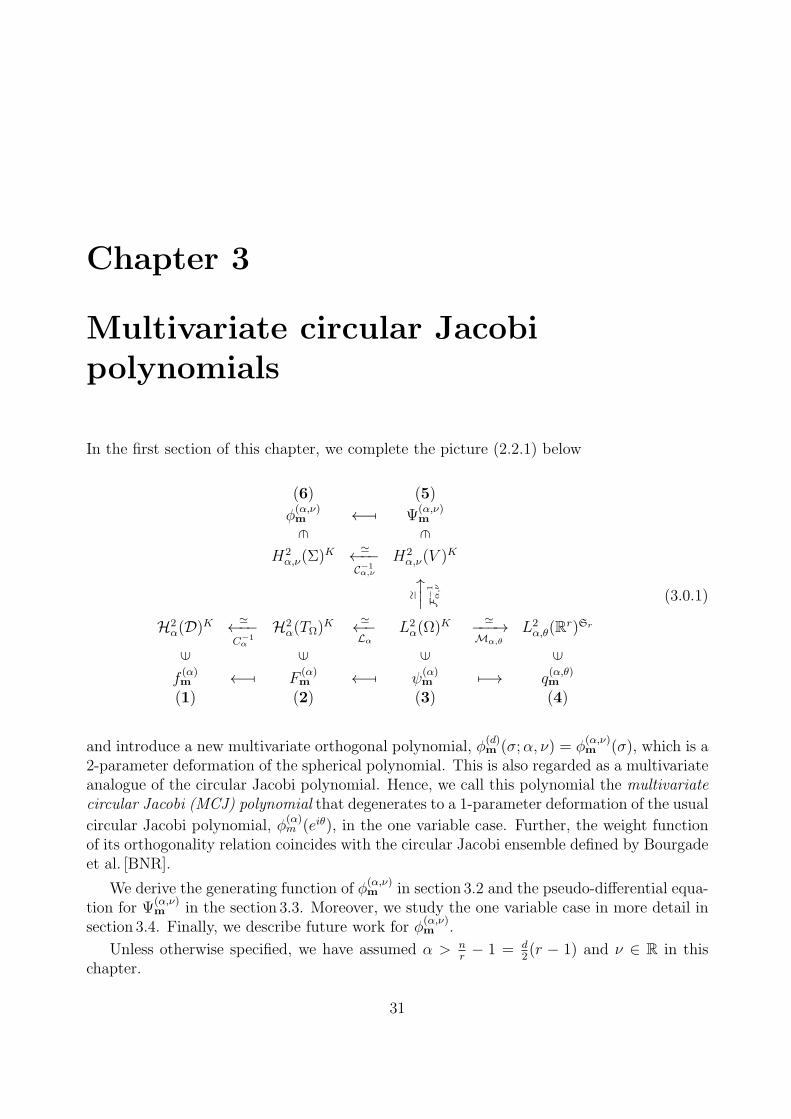
and introduce a new multivariate orthogonal polynomial, ϕ(d)m (σ;α, ν) = ϕ

(α,ν)m (σ), which is a

2-parameter deformation of the spherical polynomial. This is also regarded as a multivariateanalogue of the circular Jacobi polynomial. Hence, we call this polynomial the multivariatecircular Jacobi (MCJ) polynomial that degenerates to a 1-parameter deformation of the usual

circular Jacobi polynomial, ϕ(α)m (eiθ), in the one variable case. Further, the weight function

of its orthogonality relation coincides with the circular Jacobi ensemble defined by Bourgadeet al. [BNR].

We derive the generating function of ϕ(α,ν)m in section 3.2 and the pseudo-differential equa-

tion for Ψ(α,ν)m in the section 3.3. Moreover, we study the one variable case in more detail in

section 3.4. Finally, we describe future work for ϕ(α,ν)m .

Unless otherwise specified, we have assumed α > nr− 1 = d

2(r − 1) and ν ∈ R in this

chapter.

31

3.1 Definitions and orthogonality

Following Chapter 2, we introduce some function space, functions that become completeorthogonal bases and unitary transformations required to provide the MCJ polynomials.

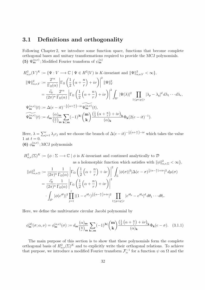
(5) Ψ(α,ν)m ;Modified Fourier transform of ψ

(α)m

H2α,ν(V )K := Ψ : V −→ C | Ψ ∈ H2(V ) is K-invariant and ∥Ψ∥2α,ν,V <∞,

∥Ψ∥2α,ν,V :=2rα

ΓΩ(α)

∣∣∣∣ΓΩ

(1

2

(α +

n

r

)+ iν

)∣∣∣∣2 ∥Ψ∥2V=

c0(2π)n

2rα

ΓΩ(α)

∣∣∣∣ΓΩ

(1

2

(α+

n

r

)+ iν

)∣∣∣∣2 ∫Rr

|Ψ(λ)|2∏

1≤p<q≤r

|λp − λq|d dλ1 · · · dλr,

Ψ(α,ν)m (t) := ∆(e− it)−

12(α+

nr )−iνΨ

(α,ν)m (t),

Ψ(α,ν)m (t) := dm

(α)m(nr

)m

∑k⊂m

(−1)|k|(m

k

)(12

(α + n

r

)+ iν

)k

(α)kΦk(2(e− it)−1).

Here, λ =∑r

j=1 λjcj and we choose the branch of ∆(e− it)−12(α+

nr )−iν which takes the value

1 at t = 0.

(6) ϕ(α,ν)m ;MCJ polynomials

H2α,ν(Σ)

K := ϕ : Σ −→ C | ϕ is K-invariant and continued analytically to Das a holomorphic function which satisfies with ∥ϕ∥2α,ν,Σ <∞,

∥ϕ∥2α,ν,Σ :=1

(2π)n1

ΓΩ(α)

∣∣∣∣ΓΩ

(1

2

(α +

n

r

)+ iν

)∣∣∣∣2 ∫Σ

|ϕ(σ)|2|∆(e− σ)12(α−n

r)+iν |2 dµ(σ)

=c0

(2π)n1

ΓΩ(α)

∣∣∣∣ΓΩ

(1

2

(α +

n

r

)+ iν

)∣∣∣∣2·∫Sr

|ϕ(eiθ)|2r∏

j=1

|(1− eiθj)12(α−

nr )+iν |2

∏1≤p<q≤r

|eiθp − eiθq |d dθ1 · · · dθr.

Here, we define the multivariate circular Jacobi polynomial by

ϕ(d)m (σ;α, ν) = ϕ(α,ν)

m (σ) := dm(α)m(nr

)m

∑k⊂m

(−1)|k|(m

k

)(12

(α + n

r

)+ iν

)k

(α)kΦk(e− σ). (3.1.1)

The main purpose of this section is to show that these polynomials form the completeorthogonal basis of H2

α,ν(Σ)K and to explicitly write their orthogonal relations. To achieve

that purpose, we introduce a modified Fourier transform F−1α for a function ψ on Ω and the

32

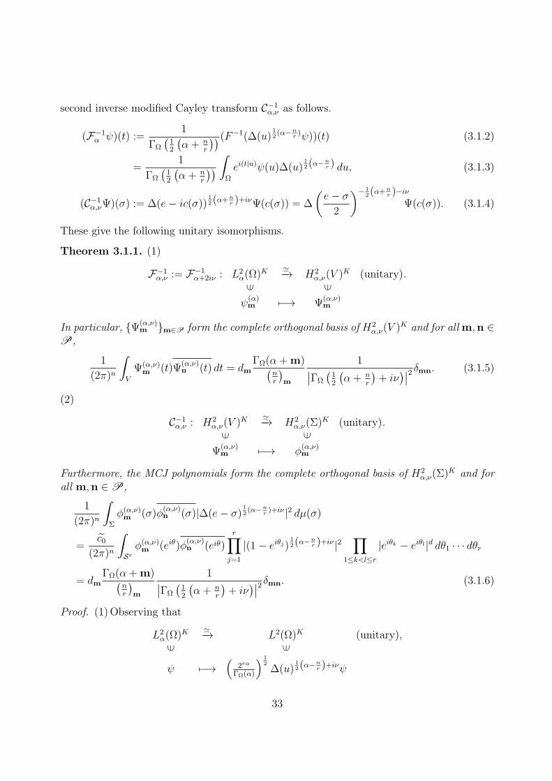
second inverse modified Cayley transform C−1α,ν as follows.

(F−1α ψ)(t) :=

1

ΓΩ

(12

(α + n

r

))(F−1(∆(u)12(α−n

r)ψ))(t) (3.1.2)

=1

ΓΩ

(12

(α + n

r

)) ∫Ω

ei(t|u)ψ(u)∆(u)12(α−

nr ) du, (3.1.3)

(C−1α,νΨ)(σ) := ∆(e− ic(σ))

12(α+

nr )+iνΨ(c(σ)) = ∆

(e− σ2

)− 12(α+

nr )−iν

Ψ(c(σ)). (3.1.4)

These give the following unitary isomorphisms.

Theorem 3.1.1. (1)

F−1α,ν := F−1

α+2iν : L2α(Ω)

K ≃−→ H2α,ν(V )K (unitary).

∈ ∈

ψ(α)m 7−→ Ψ

(α,ν)m

In particular, Ψ(α,ν)m m∈P form the complete orthogonal basis of H2

α,ν(V )K and for all m,n ∈P,

1

(2π)n

∫V

Ψ(α,ν)m (t)Ψ

(α,ν)n (t) dt = dm

ΓΩ(α +m)(nr

)m

1∣∣ΓΩ

(12

(α+ n

r

)+ iν

)∣∣2 δmn. (3.1.5)

(2)

C−1α,ν : H2

α,ν(V )K≃−→ H2

α,ν(Σ)K (unitary).

∈ ∈

Ψ(α,ν)m 7−→ ϕ

(α,ν)m

Furthermore, the MCJ polynomials form the complete orthogonal basis of H2α,ν(Σ)

K and forall m,n ∈P,

1

(2π)n

∫Σ

ϕ(α,ν)m (σ)ϕ

(α,ν)n (σ)|∆(e− σ)

12(α−n

r)+iν |2 dµ(σ)

=c0

(2π)n

∫Sr

ϕ(α,ν)m (eiθ)ϕ

(α,ν)n (eiθ)

r∏j=1

|(1− eiθj)12(α−

nr )+iν |2

∏1≤k<l≤r

|eiθk − eiθl|d dθ1 · · · dθr

= dmΓΩ(α+m)(

nr

)m

1∣∣ΓΩ

(12

(α + n

r

)+ iν

)∣∣2 δmn. (3.1.6)

Proof. (1)Observing that

L2α(Ω)

K ≃−→ L2(Ω)K (unitary),

∈ ∈

ψ 7−→(

2rα

ΓΩ(α)

) 12∆(u)

12(α−

nr )+iνψ

33

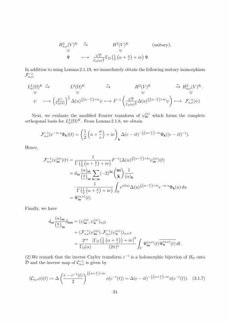
H2α,ν(V )K

≃−→ H2(V )K (unitary).

∈ ∈

Ψ 7−→ 2rα2

ΓΩ(α)12ΓΩ

(12

(α+ n

r

)+ iν

)Ψ

In addition to using Lemma2.1.19, we immediately obtain the following unitary isomorphismF−1

α,ν .

L2α(Ω)

K ≃−→ L2(Ω)K≃−→ H2(V )K

≃−→ H2α,ν(V )K .

∈ ∈ ∈ ∈

ψ 7−→(

2rα

ΓΩ(α)

) 12∆(u)

12(α−

nr )+iνψ 7−→ F−1

(2rα2

ΓΩ(α)12∆(u)

12(α−

nr )+iνψ

)7−→ F−1

α,ν(ψ)

Next, we evaluate the modified Fourier transform of ψ(α)m which forms the complete

orthogonal basis for L2α(Ω)

K . From Lemma2.1.8, we obtain

F−1α,ν(e

− tr uΦk)(t) =

(1

2

(α +

n

r

)+ iν

)k

∆(e− it)−12(α+

nr )−iνΦk((e− it)−1).

Hence,

F−1α,ν(ψ

(α)m )(t) =

1

Γ(12

(α + n

r

)+ iν

)F−1(∆(u)12(α−

nr )+iνψ(α)

m )(t)

= dm(α)m(nr

)m

∑k⊂m

(−2)|k|(m

k

)1

(α)k

· 1

Γ(12

(α + n

r

)+ iν

) ∫Ω

ei(t|u)∆(u)12(α−

nr )+iνe− tr uΦk(u) du

= Ψ(α,ν)m (t).

Finally, we have

dm(α)m(nr

)m

δmn = (ψ(α)m , ψ(α)

n )α,Ω

= (F−1α,ν(ψ

(α)m ),F−1

α,ν(ψ(α)n ))α,ν,V

=2rα

ΓΩ(α)

∣∣ΓΩ

(12

(α+ n

r

))+ iν

∣∣2(2π)n

∫V

Ψ(α,ν)m (t)Ψ

(α,ν)n (t) dt.

(2)We remark that the inverse Cayley transform c−1 is a holomorphic bijection of HΩ ontoD and the inverse map of C−1

α,ν is given by

(Cα,νϕ)(t) := ∆

(e− c−1(t)

2

) 12(α+

nr )+iν

ϕ(c−1(t)) = ∆(e− it)−12(α+

nr )−iνϕ(c−1(t)). (3.1.7)

34

Hence, since Ψ(α,ν)m m∈P form the complete orthogonal basis of H2

α,ν(V )K , it is sufficient to

show the statement for Ψ(α,ν)m m∈P and ϕ(α,ν)

m m∈P .By the definition, we have

(C−1α,νΨ

(α,ν)m )(σ) = ∆

(e− σ2

)− 12(α+

nr )−iν

∆(e− ic(σ))−12(α+

nr )−iνΨ

(α,ν)m (c(σ)) = ϕ(α,ν)

m (σ),

and from (2.1.5) of Lemma2.1.3, we have∫V

|Ψ(α,ν)m (t)|2 dt = 2n

∫Σ

|∆(e− σ)−nr |2|Ψ(α,ν)

m (c(σ))|2 dµ(σ)

= 2n∫Σ

|∆(e− σ)−nr |2∣∣∣∣∣∆(e− σ2

) 12(α+

nr )+iν

∣∣∣∣∣2

|(C−1α,νΨ

(α,ν)m )(σ)|2 dµ(σ)

= 2−rα

∫Σ

|ϕ(α,ν)m (σ)|2|∆(e− σ)

12(α−

nr )+iν |2 dµ(σ).

Therefore, we obtain

(ϕ(α,ν)m , ϕ(α,ν)

n )α,ν,Σ = (C−1α,ν(Ψ

(α,ν)m ), C−1

α,ν(Ψ(α,ν)n ))α,ν,Σ = (Ψ(α,ν)

m ,Ψ(α,ν)n )α,ν,V = dm

(α)m(nr

)m

δmn.

(3.1.6) follows from (2.1.6) of Lemma2.1.3 immediately.

Remark 3.1.2. (1)The weight function of the left hand side for (3.1.6)

r∏j=1

(1− eiθj)12(α−

nr )+iν(1− e−iθj)

12(α−

nr )−iν

∏1≤p<q≤r

|eiθp − eiθq |d

coincides with the circular Jacobi ensemble defined by [BNR].(2)When α = n

r, ν = 0, (3.1.1) and (3.1.6) degenerate to

ϕ(nr,0)

m (eiθ) = dm∑k⊂m

(−1)|k|(m

k

)Φk(e− eiθ) = dmΦm(eiθ), (3.1.8)

1

(2π)n

∫Σ

ϕ(nr,0)

m (σ)ϕ(nr,0)

n (σ) dµ(σ)

=c0

(2π)n

∫Sr

ϕ(nr,0)

m (eiθ)ϕ(nr,0)

n (eiθ)∏

1≤p<q≤r

|eiθp − eiθq |d dθ1 · · · dθr = dm1

ΓΩ

(nr

)δmn. (3.1.9)

Therefore, ϕ(α,ν)m (eiθ) is regarded as a 2-parameter deformation of the spherical polynomial.

As a generalization of spherical polynomial Φ(d)m , the Jack polynomial P

( 2d)

m which isa generalization for multiplicity d is well known (see [M], ChapterVI). This multivariatespecial orthogonal polynomial system is derived as the simultaneous eigenfunctions of some

35

commuting differential operators. On the other hand, using the unitary picture, we obtainanother extension ϕ

(α,ν)m , which is different from the Jack polynomial, that is, instead of the

multiplicity d, we consider deformations for real 2-parameters α and ν.

(3) From (2.1.31), for any θ ∈ R and m ∈P, we have

ϕ(α,ν)m (eiθe) = q

(α,− θ2)

m

(ν − i

( n2r

+ ρ))

. (3.1.10)

3.2 Generating function

By using these unitary isomorphisms, we present the generating functions of MCJ polyno-mials from (2.2.2).

Theorem 3.2.1. We assume z = u∑r

j=1 ajcj ∈ D with u ∈ U , 1 > a1 ≥ . . . ≥ ar ≥ 0 and

a1 <13.

(1)For all t ∈ V ,

∑m∈P

Ψ(α,ν)m (t)Φm(z) = ∆(e− z)−α

∫K

∆((e+ z)(e− z)−1 − ikt)−12(α+

nr )−iν dk. (3.2.1)

(2)For any σ ∈ Σ,

∑m∈P

ϕ(α,ν)m (σ)Φm(z) = ∆(e− z)−α

∫K

∆((e− z)−1 − (z(e− z)−1)kσ)−12(α+

nr )−iν dk. (3.2.2)

Proof. (1) From a similar argument to that in (2) of Lemma2.2.2,

F−1α,ν

(∑m∈P

|ψ(α)m (u)Φm(z)|

)(t) ≤ (1− a1)−r|α|−dr(r−1)F−1

α,ν(e− 1−3a1

1−a1tr u

)(t)

= (1− a1)−r|α|−dr(r−1)∆

(1− 3a11− a1

e− it)− 1

2(α+nr )−iν

<∞.

Hence, the exchange of integration and summation is justified and we obtain∑m∈P

Ψ(α,ν)m (t)Φm(z) =

∑m∈P

F−1α,ν(ψ

(α)m )(t)Φm(z)

= F−1α,ν

(∑m∈P

ψ(α)m (u)Φm(z)

)(t)

= ∆(e− z)−αF−1α,ν

(∫K

e−(ku|(e+z)(e−z)−1) dk

)(t).

36

Moreover, by Lemma2.1.8,

F−1α,ν

(∫K

e−(ku|(e+z)(e−z)−1) dk

)(t) =

1

ΓΩ

(12

(α+ n

r

)+ iν

)·∫Ω

ei(t|u)∆(u)12(α−

nr )+iν

∫K

e−(ku|(e+z)(e−z)−1) dkdu

=1

ΓΩ

(12

(α+ n

r

)+ iν

)·∫K

∫Ω

e−(u|k(e+z)(e−z)−1−it)∆(u)12(α−

nr )+iν dudk

=

∫K

∆(k(e+ z)(e− z)−1 − it)−12(α+

nr )−iν dk

=

∫K

∆((e+ z)(e− z)−1 − ikt)−12(α+

nr )−iν dk.

(2)Applying the modified Cayley transform C−1α,ν to (3.2.1), we obtain

∑m∈P

ϕ(α,ν)m (σ)Φm(z) = ∆(e− z)−αC−1

α,ν

(∫K

∆((e+ z)(e− z)−1 − ikt)−12(α+

nr )−iν dk

)(σ)

= ∆(e− z)−α∆

(e− σ2

)− 12(α+

nr )−iν

·∫K

∆((e+ z)(e− z)−1 − ikc(σ))−12(α+

nr )−iν dk.

(3.2.3)

Since

(e+ z)(e− z)−1 − ikc(σ) = 2z(e− z)−1 + 2k(e− σ)−1,

we have

∆(e− σ)−12(α+

nr )−iν

∫K

∆(z(e− z)−1 + k(e− σ)−1)−12(α+

nr )−iν dk

=

∫K

∆(e+ (k(z(e− z)−1))(e− σ))−12(α+

nr )−iν dk

=

∫K

∆(e+ (z(e− z)−1)(e− kσ))−12(α+

nr )−iν dk

=

∫K

∆((e− z)−1 − (z(e− z)−1)kσ)−12(α+

nr )−iν dk.

37

3.3 Differential equation for Ψ(α,ν)m

Considering some pseudo-differential operator that is defined by

tr (∇−1t )e(t|u) = tr (u−1)e(t|u) (any t ∈ V, u ∈ Ω), (3.3.1)

we obtain the explicit (pseudo-) differential equations for Ψ(α,ν)m as follows.

Theorem 3.3.1. The operator D(5)α,ν on V is defined by the relation D

(5)α,νF−1

α,ν = F−1α,νD

(3)α .

Then, we obtain

D(5)α,ν = tr

(−i(e+ t2)∇t +

(2ν − in

r

)t− αe+ i

(1

4

(α− n

r

)2+ ν2

)∇−1

t

), (3.3.2)

andD(5)

α,νΨ(α,ν)m (t) = 2|m|Ψ(α,ν)

m (t). (3.3.3)

Proof. From Theorem3.1.1, to prove (3.3.2), it suffices to show the relation for complete

orthogonal basis ψ(α)m for L2

α(Ω)K

(F−1α,νD

(3)α ψ(α)

m )(t) = D(5)α,ν((F−1

α,νψ(α)m )(t)),

where D(5)α,ν is the operator on the right hand side of (3.3.2).

By the very definition of the modified Fourier transform F−1α,ν and the inner product of

L2α(Ω), we can write

(F−1α,νψ)(t) = (ei(t|u)∆(u)−

12(α−

nr )+iν |ψ)L2

α(Ω), (3.3.4)

and from Lemma3.13 in [FW1], D(3)α = D

(3)α is a self-adjoint operator with respect to the

measure ∆(u)α−nr du. Hence,

(F−1α,νD

(3)α ψ(α)

m )(t) = (ei(t|u)∆(u)−12(α−

nr )+iν |D(3)

α ψ(α)m )L2

α(Ω)

= (D(3)α (ei(t|u)∆(u)−

12(α−

nr )+iν)|ψ(α)

m )L2α(Ω).

Furthermore, based on Lemma2.1.17, let us perform

tr (u∇2u)(e

i(t|u)∆(u)−12(α−

nr )+iν) = tr (u(∇2

uei(t|u)))∆(u)−

12(α−

nr )+iν

+ 2 tr (u(∇uei(t|u))(∇u∆(u)−

12(α−

nr )+iν))

+ ei(t|u) tr (u∇2u∆(u)−

12(α−

nr )+iν)

= ei(t|u)∆(u)−12(α−

nr )+iν

tr (−ut2)− i

((α− n

r

)− 2iν

)tr (t)

+

(1

2

(α− n

r

)− iν

)(1

2

(α +

n

r

)− iν

)tr (u−1)

,

38

and

tr (α∇u)(ei(t|u)∆(u)−

12(α−

nr )+iν) = α tr (∇ue

i(t|u))∆(u)−12(α−

nr )+iν

+ αei(t|u) tr (∇u∆(u)−12(α−

nr )+iν)

= tr

(iαt− α

(1

2

(α− n

r

)− iν

)u−1

)ei(t|u)∆(u)−

12(α−

nr )+iν .

Here, we remark that for any p ∈ Z≥0 tr ((∇pue

i(t|u))) = tr ((it)p)ei(t|u) and

tr (u∇2u∆(u)−

12(α−

nr )+iν) =

(−1

2

(α− n

r

)+ iν

)tr (u(∇uu

−1))∆(u)−12(α−

nr )+iν + tr (∇u∆(u)−

12(α−

nr )+iν)

=

(1

2

(α− n

r

)− iν

)(1

2

(α +

n

r

)− iν

)tr (u−1)∆(u)−

12(α−

nr )+iν

and

tr ((∇uei(t|u))(u∇u∆(u)−

12(α−

nr )+iν)) =

(−1

2

(α− n

r

)+ iν

)tr (it)ei(t|u)∆(u)−

12(α−

nr )+iν .

Hence,

D(3)α (ei(t|u)∆(u)−

12(α−

nr )+iν) = tr (−u∇2

u − α∇u + u− αe)(ei(t|u)∆(u)−12(α−

nr )+iν)

= tr

((e+ t2)u+

(2ν − in

r

)t− αe+

(1

4

(α− n

r

)2+ ν2

)u−1

)· ei(t|u)∆(u)−

12(α−

nr )+iν

= D(5)α,νe

i(t|u)∆(u)−12(α−

nr )+iν .

Therefore,

(F−1α,νD

(3)α ψ(α)

m )(t) = (D(5)α,νe

i(t|u)∆(u)−12(α−

nr )+iν |ψ(α)

m )L2α(Ω)

= D(5)α,ν(e

i(t|u)∆(u)−12(α−

nr )+iν |ψ(α)

m )L2α(Ω)

= D(5)α,ν((F−1

α,νψ)(t)).

The second equality is justified by ei(t|u)∆(u)12(α−

nr )+iνψ

(α)m ∈ L1(Ω). Finally, since F−1

α,ν is

an isomorphism from the space L2α(Ω)

K onto H2α,ν(V )K , we obtain D

(5)α,ν = D

(5)α,ν .

On the other hand, for (3.3.3), from the definition of D(5)α,ν and (2.2.6), we have

D(5)α,νΨ

(α,ν)m (t) = D(5)

α,νF−1α,ν(ψ

(α)m )(t) = F−1

α,ν(D(3)α ψ(α)

m )(t) = 2|m|F−1α,ν(ψ

(α)m )(t) = 2|m|Ψ(α,ν)

m (t).

39

We can also define D(6)α,ν by the relation D

(6)α,νC−1

α,ν = C−1α,νD

(5)α,ν . However, since there are

difficulties in deriving the modified Cayley transform of ∇−1t , we have not been able to obtain

the explicit expression for D(6)α,ν like that in the above theorem. On the other hand, when

α = nr, ν = 0, Ψ

(nr,0)

m (t) becomes

Ψ(nr,0)

m (t) = ∆(e− it)−nr dm

∑k⊂m

(−1)|k|(m

k

)Φk(2(e− it)−1)

= ∆(e− it)−nr dmΦm(c−1(t)). (3.3.5)

(3.3.6)

Further, the term of the pseudo-differential operator vanishes for D(5)nr,0. Hence,

D(5)nr,0 = −i tr ((e+ t2)∂t)−

n

rtr (e+ it). (3.3.7)

Therefore, we obtain the following explicit expression for D(6)nr,0 from the modified Cayley

transform of D(5)nr,0.

D(6)nr,0 = 2 tr (σ∇σ). (3.3.8)

3.4 One variable case

In this section, we have assumed that r = 1.First, we remark that (3.1.1) becomes

ϕ(α,ν)m (σ) :=

(α)mm!

m∑k=0

(−1)k(m

k

)(12(α+ 1) + iν

)k

(α)k(1− σ)k (3.4.1)

=(α)mm!

2F1

(−m, 1

2(α + 1) + iνα

; 1− σ)

(3.4.2)

=

(α−12− iν

)m!

2F1

(−m, 1

2(α + 1) + iν

−m− α−32

+ iν; σ

). (3.4.3)

and for α > 0, ν ∈ R, (3.1.6) degenerates to

1

2πi

∫Σ

ϕ(α,ν)m (σ)ϕ

(α,ν)n (σ)|(1− σ)

α−12

+iν |2 m(dσ)

σ=

Γ(α +m)

m!

1∣∣Γ(α+12

+ iν)∣∣2 δmn. (3.4.4)

That is a 1-parameter deformation of the usual circular Jacobi polynomial that coincideswith ϕ

(α,0)m (σ)(See [As], [Is]). In particular, ϕ

(1,0)m (σ) = σm and

1

2πi

∫Σ

ϕ(1,0)m (σ)ϕ

(1,0)n (σ)

m(dσ)

σ=

1

2π

∫ 2π

0

eimθe−inθ dθ = δmn.

40

We also remark that the rank 1 case of (3.1.10) is

ϕ(α,ν)m (eiθ) = q

(α,− θ2)

m

(ν +

1

2i

)= em

iθ2 P

(α2 )

m

(ν +

1

2i;−θ

2

), (3.4.5)

That means if θ is regarded as a parameter and ν is regarded as a variable for the circularJacobi polynomial, then we can consider the circular Jacobi polynomial to be the Meixner-Pollaczek polynomial. Moreover, the generating function of ϕ

(α,ν)m (σ) is given by∑

m≥0

ϕ(α,ν)m (σ)zm = (1− z)−

12(α−1)+iν(1− σz)−

12(α+1)−iν . (3.4.6)

Although, we have not been given an explicit expression for the differential relation ofϕ(α,ν)m (σ) in the multivariate case, we obtain the following explicit result in the one variable

case from the differential equation of 2F1.

Proposition 3.4.1. If

Dα,ν := σ(1− σ)∂2σ +(−m+

3

2+ iν

)(1− σ)− α

2(1 + σ)

∂σ +m

(1

2(α + 1) + iν

),

(3.4.7)

thenDα,νϕ

(α,ν)m (σ) = 0. (3.4.8)

3.5 Concluding remarks

We have investigated the fundamental properties of MCJ polynomials, that is, orthogonalityand the generating function etc. However, as we have not succeeded in obtaining a differentialequation for ϕ

(α,ν)m similar to Proposition 3.4.1, we can not derive a modified Cayley transform

of tr ∇−1u .

It is also important to consider the generalization of MCJ polynomials for multiplicity d.Actually, this generalization has been obtained by Baker and Forrester [BF] for multivariateLaguerre polynomials which are a modified Fourier transform of the Cayley transform ofMCJ polynomials. In addition, we can consider MCJ polynomials and their orthogonalitywithout using the analysis on the symmetric cones as follows.

Let n := r + d2r(r − 1),

dm :=Γ(d2

)rΓ(d2r) r−1∏

j=1

1

Γ(d2j)2 ∏

1≤p<q≤r

(mp −mq +

d

2(q − p)

)Γ(mp −mq +

d2(q − p+ 1)

)Γ(mp −mq +

d2(q − p− 1) + 1

) ,(3.5.1)

ΓΩ(s) := (2π)n−r2

r∏j=1

Γ

(sj −

d

2(j − 1)

),

(s)k :=r∏

j=1

(sj −

d

2(j − 1)

)kj

.

41

Further, P( 2d)

k (λ1, . . . , λr) is an r-variable Jack polynomial and

Φ(d)k (λ1, . . . , λr) :=

P( 2d)

k (λ1, . . . , λr)

P( 2d)

k (1, . . . , 1). (3.5.2)

Furthermore, we introduce the generalized (Jack) binomial coefficients based on [OO] by

Φ(d)m (1 + λ1, . . . , 1 + λr) =

∑k⊂m

(m

k

)d2

Φ(d)k (λ1, . . . , λr).

Definition 3.5.1. We define the generalized MCJ polynomial as follows.

ϕ(d)m (eiθ;α, ν) = ϕ(d)

m (eiθ1 , . . . , eiθr ;α, ν) := dm(α)m(nr

)m

∑k⊂m

(−1)|k|(m

k

)d2

(12

(α + n

r

)+ iν

)k

(α)k

· Φ(d)k (1− eiθ1 , . . . , 1− eiθr). (3.5.3)

Therefore, we present the following conjecture.

Conjecture 3.5.2. If α > nr− 1, ν ∈ R, d > 0, then

c0(2π)n

∫Sr

ϕ(d)m (eiθ;α, ν)ϕ

(d)n (eiθ;α, ν)

r∏j=1

|(1− eiθj)12(α−

nr )+iν |2

∏1≤p<q≤r

|eiθp − eiθq |d dθ1 · · · dθr

= dmΓΩ(α +m)(

nr

)m

1∣∣ΓΩ

(12

(α + n

r

)+ iν

)∣∣2 δmn. (3.5.4)

For some special case, we prove the conjecture.

Proposition 3.5.3. (1) If d = 1, 2, 4 or r = 2, d ∈ Z>0 or r = 3, d = 8, then this conjectureis true.

(2)The case of α = nrand ν = 0 is also true.

Proof. (1) It follows immediately from Theorem3.1.1 and the classification of irreduciblesymmetric cones.

(2)We remark that when α = nr, ν = 0,

ϕ(d)m

(eiθ;

n

r, 0)= dm

∑k⊂m

(−1)|k|(m

k

)d2

P( 2d)

k (1− eiθ1 , . . . , 1− eiθr)

P( 2d)

k (1, . . . , 1)

= dmP

( 2d)

m (eiθ1 , . . . , eiθr)

P( 2d)

m (1, . . . , 1). (3.5.5)

42

For the Jack polynomial, the following formulas are known (see (6.4) in [OO] and (10.38) in[M] respectively).

P( 2d)

m (1, . . . , 1) =r∏

j=1

Γ(d2

)Γ(d2j) ∏

1≤p<q≤r

Γ(mp −mq +

d2(q − p+ 1)

)Γ(mp −mq +

d2(q − p)

) , (3.5.6)

∥P (2d)

m ∥2r, 2

d:=

1

(2π)r1

r!

∫Sr

|P (2d)

m (eiθ1 , . . . , eiθr)|2∏

1≤p<q≤r

|eiθp − eiθq |d dθ1 · · · dθr

=∏

1≤p<q≤r

Γ(mp −mq +

d2(q − p+ 1)

)Γ(mp −mq +

d2(q − p− 1) + 1

)Γ(mp −mq +

d2(q − p)

)Γ(mp −mq +

d2(q − p) + 1)

) .

(3.5.7)

Hence, from (3.5.1), (3.5.6) and (3.5.7), we have

dm∥P( 2d)

m ∥2r, 2

d=

Γ(d2r)

Γ(d2

)r P ( 2d)

m (1, . . . , 1)2. (3.5.8)

Therefore, by (3.5.5) and the orthogonality of the Jack polynomial, we obtain

c0(2π)n

∫Sr

ϕ(d)m

(eiθ;

n

r, 0)ϕ(d)n

(eiθ;

n

r, 0) ∏

1≤p<q≤r

|eiθp − eiθq |d dθ1 · · · dθr

=1

(2π)n(2π)

n−r2

r!

r∏

j=1

Γ(d2

)Γ(d2j) d2m

P( 2d)

m (1, . . . , 1)2(2π)rr!∥P (

2d)

m ∥2r, 2

dδmn

=dm

(2π)n−r2

r−1∏j=1

1

Γ(d2j)δmn = dm

1

ΓΩ

(nr

)δmn.

Although a proof of a general case would be desirable, our method in this thesis cannotbe applied to a general case. It may be necessary to consider a method of quantum integrablesystems, that is, to construct some commuting families of differential or pseudo-differentialoperators whose simultaneous eigenfunctions become MCJ polynomials. We are not awareof any studies of constructions of commuting families of pseudo-differential operators thusfar. Hence, we think our conjecture is likely to be an important target of investigations intoquantum integrable systems. Since multivariate Laguerre polynomials have been studied byusing degenerate double affine Hecke algebra [Ka], we are also interested in similar algebraictreatment of MCJ polynomials which are the composition of modified Cayley and Fouriertransforms of multivariate Laguerre polynomials.

Finally, we would like to raise the issue of applications for MCJ polynomials. In partic-ular, since the weight function of the orthogonality relation for MCJ polynomials coincideswith a circular Jacobi ensemble, we expect an application to the random matrix model whosedensity function is a circular Jacobi ensemble. However, further details on this are goals offuture work.

43

Chapter 4

Multivariate Meixner, Charlier andKrawtchouk polynomials

The standard Meixner, Charlier and Krawtchouk polynomials of single discrete variable aredefined by

Mm(x;α, c) := 2F1

(−m,−x

α; 1− 1

c

)=

m∑k=0

k!

(α)k

(m

k

)(x

k

)(1− 1

c

)k

,

Cm(x; a) := 2F0

(−m,−x− ;−1

a

)=

m∑k=0

(m

k

)(x

k

)(−1

a

)k

,

Km(x; p,N) := 2F1

(−m,−x−N ;

1

p

)=

m∑k=0

k!

(−N)k

(m

k

)(x

k

)(1

p

)k

,

respectively. These polynomials have been generalized to the multivariate case [DG], [Gr1],[Gr2], and [Il]. Although these multivariate discrete orthogonal polynomials are types writtenin Aomoto-Gelfand hypergeometric series, we introduce other types of multivariate Meixner,Charlier and Krawtchouk polynomials in this chapter, which are defined by generalizedbinomial coefficients. Moreover, we provide their fundamental properties, that is, duality,degenerate limits, generating functions, orthogonality relations, difference equations andrecurrence formulas. The most basic result in these properties is Theorem4.2.2, whichstates that the generating function of the generating functions for the multivariate Meixnerpolynomials ∑

x∈P

dx1(nr

)x

∑m∈P

dm(α)m(nr

)m

Mm(x;α, c)Φm(z)

Φx(w)

coincides with the generating function for the multivariate Laguerre polynomials

∑m∈P

etr wL(α−n

r )m

((1

c− 1

)w

)Φm(z).

44

Even though this result has not been known even for one variable, many properties for ourmultivariate discrete special orthogonal polynomials follow from this and the unitary picture(3.0.1).

In this chapter, we assume that m,n,x,y ∈ P, α ∈ C, 0 < c, p < 1, a > 0, N ∈ Z≥0

unless otherwise specified.

4.1 Definitions

Definition 4.1.1. We define the multivariate Meixner, Charlier and Krawtchouk polyno-mials as follows.

Mm(x;α, c) :=∑k⊂m

1

dk

(nr

)k

(α)k

(m

k

)(x

k

)(1− 1

c

)|k|

(4.1.1)

=∑k⊂m

(m

k

)γk(x− ρ)

(α)k

(1− 1

c

)|k|

(4.1.2)

=∑k⊂m

dkγk(m− ρ)γk(x− ρ)(

nr

)k(α)k

(1− 1

c

)|k|

, (4.1.3)

Cm(x; a) :=∑k⊂m

1

dk

(nr

)k

(m

k

)(x

k

)(−1

a

)|k|

(4.1.4)

=∑k⊂m

(m

k

)γk(x− ρ)

(−1

a

)|k|

(4.1.5)

=∑k⊂m

dkγk(m− ρ)γk(x− ρ)(

nr

)k

(−1

a

)|k|

, (4.1.6)

Km(x; p,N) :=∑k⊂m

1

dk

(nr

)k

(−N)k

(m

k

)(x

k

)(1

p

)|k|

(m ⊂ N = (N, . . . , N)) (4.1.7)

=∑k⊂m

(m

k

)γk(x− ρ)(−N)k

(1

p

)|k|

(4.1.8)

=∑k⊂m

dkγk(m− ρ)γk(x− ρ)(

nr

)k(−N)k

(1

p

)|k|

. (4.1.9)

When r = 1, these polynomials become the usual Meixner, Charlier and Krawtchoukpolynomials. By the definition, we immediately obtain a duality property for these polyno-mials.

Proposition 4.1.2. (1)For all m,x ∈P, we have

Mm(x;α, c) =Mx(m;α, c). (4.1.10)

45

(2)For all m,x ∈P, we haveCm(x; a) = Cx(m; a). (4.1.11)

(3)For all N ⊃m,x ∈P, we have

Km(x; p,N) = Kx(m; p,N). (4.1.12)

We also obtain the following relations by the definitions.

Proposition 4.1.3. (1)

Mm

(x;−N, p

p− 1

)= Km(x; p,N). (4.1.13)

(2)

limα→∞

Mm

(x;α,

a

a+ α

)= Cm(x; a). (4.1.14)

(3)

limN→∞

Km

(x;

a

N,N)= Cm(x; a). (4.1.15)

Actually, (1) follows from the definitions. For (2) and (3), we remark that

limα→∞

α|k|

(α)k= lim

α→∞

r∏j=1

αkj(α− d

2(j − 1)

)kj

= 1,

limN→∞

N |k|

(−N)k= lim

N→∞

r∏j=1

Nkj(−N − d

2(j − 1)

)kj

= (−1)|k|.

4.2 Generating functions

In this chapter, we put

z = u1

r∑j=1

ajcj, w = u2

r∑j=1

bjcj ∈ V C,

with u1, u2 ∈ U , a1 ≥ · · · ≥ ar ≥ 0, b1 ≥ · · · ≥ br ≥ 0 unless otherwise specified.To consider some generating functions of generating functions for the above polynomials,

we need to prove their convergences.

Lemma 4.2.1. (1) If 1 > a1 ≥ · · · ≥ ar ≥ 0, b1 ≥ · · · ≥ br ≥ 0, then∑x,m∈P

∣∣∣∣∣dm (α)m(nr

)m

Mm(x;α, c)Φm(z)dx1(nr

)x

Φx(w)

∣∣∣∣∣ ≤ erb1

(1+

a11−a1

( 1c−1)

)(1− a1)−r(|α|+2n).

(4.2.1)(2)For any z, w ∈ V C, we have∑

x,m∈P

∣∣∣∣∣dm 1(nr

)m

Cm(x, a)Φm(z)dx1(nr

)x

Φx(w)

∣∣∣∣∣ ≤ er(a1+b1+a1b1a ). (4.2.2)

46

Proof. (1) By Lemma2.1.5, Lemma2.1.10 and Lemma2.1.15,

∑x,m∈P

∣∣∣∣∣dm (α)m(nr

)m

Mm(x;α, c)Φm(z)dx1(nr

)x

Φx(w)

∣∣∣∣∣≤∑k∈P

dk1(

nr

)k(|α|+ d(r − 1))k

(1

c− 1

)|k|

·∑m∈P

dm(|α|+ d(r − 1))m(

nr

)m

γk(m− ρ)Φm(a1)∑x∈P

dx1(nr

)x

γk(x− ρ)Φx(b1).

Moreover, from (2.1.38) and (2.1.39) of Theorem2.1.16,

∑m∈P

dm(|α|+ d(r − 1))m(

nr

)m

γk(m− ρ)Φm(a1) = (|α|+ d(r − 1))k(1− a1)−r|α|−dr(r−1)

(a1

1− a1

)|k|

,

∑x∈P

dx1(nr

)x

γk(x− ρ)Φx(b1) = erb1b1|k|.

Therefore, we have

∑x,m∈P

∣∣∣∣∣dm (α)m(nr

)m

Mm(x;α, c)Φm(z)dx1(nr

)x

Φx(w)

∣∣∣∣∣≤ erb1(1− a1)−r(|α|+d(r−1))

∑k∈P

dk1(nr

)k

Φk

((1

c− 1

)a1b11− a1

)= e

rb1(1+

a11−a1

( 1c−1)

)(1− a1)−r(|α|+d(r−1)) <∞.

(2)By a similar argument,

∑x,m∈P

∣∣∣∣∣dm 1(nr

)m

Cm(x, a)Φm(z)dx1(nr

)x

Φx(w)

∣∣∣∣∣≤∑k∈P

dk1(nr

)k

a−|k|∑m∈P

dm1(nr

)m

γk(m− ρ)Φm(a1)∑x∈P

dx1(nr

)x

γk(x− ρ)Φx(b1)

= er(a1+b1)∑k∈P

dk1(nr

)k

Φk

(a1b1a

)= er(a1+b1+

a1b1a ) <∞.

The following theorem is the key result in our theory.

47

Theorem 4.2.2. (1) For z ∈ D, w ∈ V C, α ∈ C, 0 < c < 1, we obtain∑m∈P

etr wL(α−n

r )m

((1

c− 1

)w

)Φm(z) =

∑x,m∈P

dm(α)m(nr

)m

Mm(x;α, c)Φm(z)

· dx1(nr

)x

Φx(w) (4.2.3)

= ∆(e− z)−α

∫K

e(kw|(e− 1cz)(e−z)−1) dk. (4.2.4)

(2)For w, z ∈ V C, a > 0, we obtain∑m∈P

dm1(nr

)m

etr wΦm

(e− 1

aw

)Φm(z) =

∑x,m∈P

dm1(nr

)m

Cm(x; a)Φm(z)

· dx1(nr

)x

Φx(w) (4.2.5)

= etr (w+z)

∫K

e−1a(kw|z) dk. (4.2.6)

Proof. (1) By the above lemma, the series converges absolutely under the conditions. There-fore, we derive∑

x,m∈P

dm(α)m(nr

)m

Mm(x;α, c)Φm(z)dx1(nr

)x

Φx(w)

=∑m∈P

dm(α)m(nr

)m

Φm(z)∑k⊂m

(m

k

)1

(α)k

(1− 1

c

)|k| ∑x∈P

dx1(nr

)x

γk(x− ρ)Φx(w)

=∑m∈P

etr wdm(α)m(nr

)m

∑k⊂m

(m

k

)(−1)k

(α)kΦk

((1

c− 1

)w

)Φm(z)

=∑m∈P

etr wL(α−n

r )m

((1

c− 1

)w

)Φm(z).

(4.2.4) follows from (2.2.2).(2) Put c = a

a+α, w → w

α, a, α ∈ R>0 in (1) of Theorem4.2.2 and take the limit of α→∞.

The generating functions of our polynomials are a corollary of the above theorem.

Theorem 4.2.3. (1) For z ∈ D,x ∈P, α ∈ C, 0 < c < 1, we have

∆(e− z)−αΦx

((e− 1

cz

)(e− z)−1

)=∑n∈P

dn(α)n(nr

)n

Mn(x;α, c)Φn(z). (4.2.7)

(2) For z ∈ D,x ∈P, a > 0, we have

etr zΦx

(e− 1

az

)=∑n∈P

dn1(nr

)n

Cn(x; a)Φn(z). (4.2.8)

48

(3) For z ∈ D,x ∈P, 0 < p < 1, we have

∆(e+ z)NΦx

((e− 1− p

pz

)(e+ z)−1

)=∑n⊂N

(N

n

)Kn(x; p,N)Φn(z). (4.2.9)

Proof. (1)We evaluate the spherical Taylor expansion of (4.2.4) with respect to w:

Φx(∂w)∆(e− z)−α

∫K

e(kw|(e− 1cz)(e−z)−1) dk

∣∣∣∣w=0

= ∆(e− z)−α

∫K

Φx(∂w)e(w|k(e− 1

cz)(e−z)−1)|w=0 dk

= ∆(e− z)−α

∫K

Φx

(k

((e− 1

cz

)(e− z)−1

))dk

= ∆(e− z)−αΦx

((e− 1

cz

)(e− z)−1

).

On the other hand, by (4.2.3),

Φx(∂w)∆(e− z)−α

∫K

e(kw|(e− 1cz)(e−z)−1) dk

∣∣∣∣w=0

=∑n∈P

dn(α)n(nr

)n

Mn(x;α, c)Φn(z).

Therefore, we obtain the conclusion.(2) The result is proved by a similar argument as in (1). That is, by (2) of Theorem4.2.2,we have ∑

n∈P

dn1(nr

)n

Cn(x; a)Φn(z) = Φx(∂w)etr (w+z)

∫K

e−1a(kw|z) dk

∣∣∣∣w=0

= etr z

∫K

Φx(∂w)e(w|k(e− 1

az))|w=0 dk

= etr z

∫K

Φx

(k

(e− 1

az

))dk

= etr zΦx

(e− 1

az

).

(3)By putting α = −N in (4.2.3), we have

∆(e− z)NΦx

((e− 1

cz

)(e− z)−1

)=∑n⊂N

dn(−N)n(

nr

)n

Mn(x;−N, c)Φn(z)

=∑n⊂N

(N

n

)Mn(x;−N, c)Φn(−z).

Since this series is a finite sum, we can take c = pp−1

in the above. Therefore, we obtain

∆(e− z)NΦx

((e+

1− pp

z

)(e− z)−1

)=∑n⊂N

(N

n

)Mn

(x;−N, p

p− 1

)Φn(−z)

=∑n⊂N

(N

n

)Kn (x; p,N) Φn(−z).

49

Next, we apply the unitary transformations in (3.0.1) to Theorem4.2.2. Here, we alsocheck convergence.

Lemma 4.2.4. (1)Fix 0 < c < 1 and let 0 < ε < 1 and w, z ∈ D satisfy that(c+ (1− c) ε

1− ε

)(1 + (1− c) ε

1− cε

)< 1,

|Φm(w)|, |Φm(z)| < Φm(ε) = ε|m|. (4.2.10)

Then,

∑x,m,n∈P

∣∣∣∣∣dx (α)x(nr

)x

c|x|dm(α)m(nr

)m

Mm(x;α, c)Φm(z)dn(α)n(nr

)n

Mn(x;α, c)Φn(cw)

∣∣∣∣∣< ((1− c)(1− 2(1 + c)ε+ (4c− 1)ε2))−r|α|−dr(r−1). (4.2.11)

(2)Let z ∈ D satisfy that

√c+

1− c√c

a11− a1

< 1, |Φm(z)| ≤ a1|m|. (4.2.12)

Under this condition, the series

∑x,m∈P

dm(α)m(nr

)m

Mm(x;α, c)Φm(z)dx1(nr

)x

γx

(−is− α

2

)(c(1− e2iθ)e2iθ − c

)|x|

(4.2.13)

and

∑x,m∈P

dm(α)m(nr

)m

Mm(x;α, c)Φm(z)dx

(12

(α + n

r

)+ iν

)x(

nr

)x

c|x|Φx((e− σ)(e− cσ)−1) (4.2.14)

converge absolutely for any s ∈ Rr and σ ∈ Σ respectively.

Proof. (1) By Lemma2.1.5 and Lemma2.1.15, we have

(LHS) ≤∑x∈P

dx(|α|+ d(r − 1))x(

nr

)x

c|x|

·∑k⊂x

(x

k

)1

(|α|+ d(r − 1))k

(1

c− 1

)|k|∑l⊂x

(x

l

)1

(|α|+ d(r − 1))l

(1

c− 1

)|l|

·∑m∈P

dm(|α|+ d(r − 1))m(

nr

)m

γk(m− ρ)Φm(ε)∑n∈P

dn(|α|+ d(r − 1))n(

nr

)n

γl(n− ρ)Φn(cε).

50

Furthermore, from Lemma2.1.16 and the definition of the generalized binomial coefficients(2.1.24), we derive

(LHS) ≤ ((1− ε)(1− cε))−r|α|−dr(r−1)∑x∈P

dx(|α|+ d(r − 1))x(

nr

)x

c|x|

·∑k⊂x

(x

k

)(1

c− 1

)|k|

Φk

(ε

1− ε

)∑l⊂x

(x

l

)(1

c− 1

)|l|

Φl

(cε

1− cε

)= ((1− ε)(1− cε))−r|α|−dr(r−1)

·∑x∈P

dx(|α|+ d(r − 1))x(

nr

)x

Φx

((c+ (1− c) ε

1− ε

)(1 + (1− c) ε

1− cε

)).

Finally, by using the assumption and Lemma2.1.16, we obtain

(LHS) ≤((1− ε)(1− cε)

(1−

(c+ (1− c) ε

1− ε

)(1 + (1− c) ε

1− cε

)))−r|α|−dr(r−1)

= ((1− c)(1− 2(1 + c)ε+ (4c− 1)ε2))−r|α|−dr(r−1).

(2) For (4.2.13), by a similar argument as that above, we obtain∑x,m∈P

∣∣∣∣∣dm (α)m(nr

)m

Mm(x;α, c)Φm(z)dx1(nr

)x

γx

(−is− α

2

)(c(1− e2iθ)e2iθ − c

)|x|∣∣∣∣∣

≤∑x∈P

dx1(nr

)x

∣∣∣γx (−is− α

2

)∣∣∣ ( 2c

1 + c

)|x|∑k⊂x

(x

k

)1

(|α|+ d(r − 1))k

(1

c− 1

)|k|

·∑m∈P

dm(|α|+ d(r − 1))m(

nr

)m

γk(m− ρ)Φm(a1)

≤ (1− a1)−r|α|−dr(r−1)∑x∈P

dx1(nr

)x

∣∣∣γx (−is− α

2

)∣∣∣ c |x|2

∑k⊂x

(x

k

)Φk

((1

c− 1

)a1

1− a1

)≤ (1− a1)−r|α|−dr(r−1)

∑x∈P

dx1(nr

)x

∣∣∣γx (−is− α

2

)∣∣∣Φx

(√c+

1− c√c

a11− a1

).

Finally, by Lemma2.1.14,

≤ C1 + C2(1− a1)−r|α|−dr(r−1)∑x∈P

dx(|α|+ d(r − 1))x(

nr

)x

Φx

(√c+

1− c√c

a11− a1

)

≤ C1 + C2

((1−

√c)

(1− a1 −

(1 +

1√c

)a1

))−r|α|−dr(r−1)

.

For (4.2.14), by using σ =∑r

j=1 eiθjcj and

|(e− σ)(e− cσ)−1)| ≤r∑

j=1

∣∣∣∣ 1− eiθj1− ceiθj

∣∣∣∣ cj ≤ r∑j=1

2

1 + ccj =

2

1 + c≤ 1√

c,

51

we have∑x,m∈P

∣∣∣∣∣dm (α)m(nr

)m

Mm(x;α, c)Φm(z)dx

(12

(α + n

r

)+ iν

)x(

nr

)x

c|x|Φx((e− σ)(e− cσ)−1)

∣∣∣∣∣≤∑x∈P

dx

(12

(|α|+ n

r

)+ |ν|+ d(r − 1)

)x(

nr

)x

Φx(√c)

·∑k⊂x

(x

k

)1

(|α|+ d(r − 1))k

(1

c− 1

)|k| ∑m∈P

dm(|α|+ d(r − 1))m(

nr

)m

γk(m− ρ)Φm(a1)

= (1− a1)−r|α|−dr(r−1)∑x∈P

dx

(12

(|α|+ n

r

)+ |ν|+ d(r − 1)

)x(

nr

)x

Φx(√c)

·∑k⊂x

(x

k

)Φk

((1

c− 1

)a1

1− a1

)

= (1− a1)−r|α|−dr(r−1)∑x∈P

dx

(12

(|α|+ n

r

)+ |ν|+ d(r − 1)

)x(

nr

)x

Φx

(√c+

1− c√c

a11− a1

)= (1− a1)−r|α|−dr(r−1)

((1−

√c)

(1−

(1 +

1√c

)a1

1− a1

))<∞.

From this lemma, we can consider the following generating functions.

Theorem 4.2.5. (1)For z ∈ D, u ∈ V C, we obtain∑m∈P

ψ(α)m (u)Φm(z) =

∑x,m∈P

dm(α)m(nr

)m

Mm(x;α, c)Φm(z)

· dx1(nr

)x

(2c

1− c

)|x|

e−1+c1−c

tr uΦx(u) (4.2.15)

= ∆(e− z)−α

∫K

e−(ku|(e+z)(e−z)−1) dk.

(2)Fixed 0 < c < 1 and assume that w, z ∈ D satisfy the condition in (1) of Lemma4.2.4.We obtain∑

m∈P

dm(α)m(nr

)m

Φm(w)Φm(z) = (1− c)rα∑

x,m∈P

dm(α)m(nr

)m

Mm(x;α, c)Φm(z)

· dx(α)x(nr

)x

c|x|∆(e− cw)−αΦx((e− w)(e− cw)−1) (4.2.16)

= ∆(z)−α

∫K

∆(kz−1 − w)−α dk.

52

(3)Fixed 0 < c < 1 and assume that z ∈ D satisfy the condition in (2) of Lemma4.2.4. Fors ∈ Rr, 0 < θ < 2π, we obtain

∑m∈P

q(α)m (s; θ)Φm(z) =

(1− c

1− ce−2iθ

)−i|s|−α2r ∑x,m∈P

dm(α)m(nr

)m

Mm(x;α, c)Φm(z)

· dx1(nr

)x

γx

(−is− α

2

)(c(1− e2iθ)e2iθ − c

)|x|

(4.2.17)

= ∆(e− z)−αφis+α2((e− e−2iθz)−1(e− z)).

(4)Fixed 0 < c < 1 and assume that z ∈ D satisfy the condition in (2) of Lemma4.2.4. Forσ ∈ Σ, we obtain∑m∈P

ϕ(α,ν)m (σ)Φm(z) = (1− c)

r2(α+

nr )+irν

∑x,m∈P

dm(α)m(nr

)m

Mm(x;α, c)Φm(z)

· dx

(12

(α+ n

r

)+ iν

)x(

nr

)x

c|x|∆(e− cσ)−12(α+

nr )−iνΦx((e− σ)(e− cσ)−1)

(4.2.18)

= ∆(e− z)−α

∫K

∆((e− z)−1 − (z(e− z)−1)kσ)−12(α+

nr )−iν dk.

(5)For w, z ∈ V C, a > 0, we obtain

∑m∈P

dm1(nr

)m

Φm(w)Φm(z) = e−ra∑

x,m∈P

dma|m|(nr

)m

Cm(x; a)Φm(z)

· dxa|x|(nr

)x

etr wΦx

(e− 1

aw

)(4.2.19)

= etr w

∫K

e−a(kw|e−z) dk.

Proof. As (1) and (5) follow immediately from Theorem4.2.2, we only prove (2), (3) and(4).

First, we remark that the right hand sides of (4.2.16), (4.2.17) and (4.2.18) convergeabsolutely under the conditions in Lemma4.2.4. Thus, by analytic continuation, it sufficesto show these equations when a1 <

13. Moreover, we also remark that since (2.2.4)∑

m∈P

|ψ(α)m (u)Φm(z)| ≤ (1− a1)−r|α|−dr(r−1)e

− 1−3a11−a1 ,

the exchange of unitary transformations Lα,Mα,θ and F−1α,ν , and the summation are justified

under these restrictions. Therefore, to obtain the results, we apply the unitary transformsto both sides of (4.2.15). We try to perform these calculations.

53

For (2), we apply transform C−1α Lα to both sides of (4.2.15). From Lemma2.1.8, we

have

Lα(e− 1+c

1−ctr uΦx)(z) =

2rα

ΓΩ(α)

∫Ω

e−(

1+c1−c

e+z

∣∣u)Φx(u)∆(u)α−

nr du

= 2rα(α)x∆

(1 + c

1− ce+ z

)−α

Φx

((1 + c

1− ce+ z

)−1).

Furthermore,

C−1α Lα(e

− 1+c1−c

tr uΦx)(w) = 2rα(α)xC−1α

(∆

(1 + c

1− ce+ z

)−α

Φx

((1 + c

1− ce+ z

)−1))

(w)

= (α)x∆(e− w)−α∆

(1

2

((e+ w)(e− w)−1 +

1 + c

1− ce

))−α

· Φx

(((e+ w)(e− w)−1 +

1 + c

1− ce

)−1)

= (α)x(1− c)rα∆(e− cw)−αΦx

(1− c2

(e− w)(e− cw)−1

).

Hence, the right-hand side of (4.2.15) becomes the right-hand side of (4.2.16). Therefore,

since C−1α Lα(ψm(α))(w) = dm

(α)m

(nr )m

Φm(w), we obtain the conclusion.

By similar arguments, for (3) and (4), we only need to evaluate the following calculations.(2c

1− c

)|x|

Mα,θ(e− 1+c

1−ctr uΦx)(s) =

(1− c

1− ce−2iθ

)−i|s|−α2r

γx

(−is− α

2

)(c(1− e2iθ)e2iθ − c

)|x|

,(2c

1− c

)|x|

C−1α,ν F−1

α,ν(e− 1+c

1−ctr uΦx)(σ) = (1− c)

r2(α+

nr )+irν

(1

2

(α+

n

r

)+ iν

)x

· c|x|∆(e− cσ)−12(α+

nr )−iνΦx((e− σ)(e− cσ)−1)

These follow from Lemma2.1.12 and Lemma2.1.8.

4.3 Orthogonality relations

We provide the orthogonality relations for our discrete orthogonal polynomials as a corollaryof Theorem4.2.5.

Theorem 4.3.1. (1) For α > nr− 1, 0 < c < 1, we obtain

∑x∈P

dx(α)x(nr

)x

c|x|Mm(x;α, c)Mn(x;α, c) =c−|m|

(1− c)rα1

dm

(nr

)m

(α)mδm,n ≥ 0. (4.3.1)

54

(2) For a > 0, we obtain

∑x∈P

dxa|x|(nr

)x

Cm(x; a)Cn(x; a) = a−|m|era(nr

)m

dmδm,n ≥ 0. (4.3.2)

(3) For 0 < p < 1, we obtain

∑x⊂N

(N

x

)p|x|(1− p)rN−|x|Km(x; p,N)Kn(x; p,N) =

(1− pp

)|m|(N

m

)−1

δm,n ≥ 0. (4.3.3)

Proof. (1) From (4.2.16) and (4.2.7), we have

∑m∈P

dm(α)m(nr

)m

Φm(w)Φm(z) = (1− c)rα∑

x,m∈P

dm(α)m(nr

)m

Mm(x;α, c)Φm(z)

· dx(α)x(nr

)x

c|x|∆(e− cw)−αΦx((e− w)(e− cw)−1)

=∑

m,n∈P

(1− c)rαdm(α)m(nr

)m

dn(α)n(nr

)n

c|n|

·

∑x∈P

dx(α)x(nr

)x

c|x|Mm(x;α, c)Mn(x;α, c)

Φm(z)Φn(w).

Therefore, by comparing the coefficients of Φm(z)Φn(w) on both sides of this equation, weobtain (4.3.1).

(2) From (4.2.19) and (4.2.8), we derive

∑m∈P

dm1(nr

)m

Φm(w)Φm(z) = e−ra∑

x,m∈P

dma|m|(nr

)m

Cm(x; a)Φm(z)

· dxa|x|(nr

)x

etr wΦx

(e− 1

aw

)=

∑m,n∈P

e−radma|m|(nr

)m

dn1(nr

)n

·

∑x∈P

dxa|x|(nr

)x

Cm(x; a)Cn(x; a)

Φm(z)Φn(w).

Then, by comparing the coefficients of Φm(z)Φn(w), we have the conclusion.

55

(3) In (4.2.16), taking α = −N , one has

∑m⊂N

dm(−N)m(

nr

)m

Φm(w)Φm(−z) =∑m⊂N

(N

m

)Φm(w)Φm(z)

= (1− c)−rN∑

x,m⊂N

dm(−N)m(

nr

)m

Mm(x;−N, c)Φm(−z)

· dx(−N)x(

nr

)x

c|x|∆(e− cw)NΦx((e− w)(e− cw)−1).

The first equality follows from (2.1.31). Since the above sum is finite, we can put c =p

p−1, (0 < p < 1). Hence,

∑m⊂N

(N

m

)Φm(w)Φm(z) = (1− p)rN

∑x,m⊂N

(N

m

)Km(x; p,N)Φm(z)

(N

x

)(p

1− p

)|x|

·∆(e+

p

1− pw

)N

Φx

((e− w)

(e+

p

1− pw

)−1).

From (4.2.9), we have

∆

(e+

p

1− pw

)N

Φx

((e− w)

(e+

p

1− pw

)−1)

=∑n⊂N

(N

n

)Kn(x; p,N)

(p

1− p

)|n|

Φn(w).

Therefore,

∑m⊂N

(N

m

)Φm(w)Φm(z) =

∑m,n⊂N

(N

m

)(p

1− p

)|n|(N

n

)

·

∑x⊂N

(N

x

)p|x|(1− p)rN−|x|Km(x; p,N)Kn(x; p,N)

Φm(z)Φn(w).

4.4 Difference equations and recurrence relations

In this section, we derive the difference equations and recurrence formulas for our polynomialsfrom (2.2.6), Lemma2.2.3 and (1) of Theorem4.2.5.

56

Theorem 4.4.1. (1) For x,m ∈P, α ∈ C, c ∈ C∗, we have

dx(c− 1)|m|Mm(x;α, c) =r∑

j=1

dx+ϵj aj(−x− ϵj)(xj + α− d

2(j − 1)

)cMm(x+ ϵj;α, c)

−r∑

j=1

dx(xj + (xj + α)c)Mm(x;α, c)

+r∑

j=1

dx−ϵj aj(x− ϵj)(xj +

d

2(r − j)

)Mm(x− ϵj;α, c). (4.4.1)

(2) For x,m ∈P, a ∈ C∗, we have

−dx|m|Cm(x; a) =r∑

j=1

dx+ϵj aj(−x− ϵj)aCm(x+ ϵj; a)

−r∑

j=1

dx(xj + a)Cm(x; a)

+r∑

j=1

dx−ϵj aj(x− ϵj)(xj +

d

2(r − j)

)Cm(x− ϵj; a). (4.4.2)

(3) For x,m ∈P, p ∈ C∗, we have

−dx|m|Km(x; p,N) =r∑

j=1

dx+ϵj aj(−x− ϵj)(N − xj +

d

2(j − 1)

)pKm(x+ ϵj; p,N)

−r∑

j=1

dx(p(N − xj) + xj(1− p))Km(x; p,N)

+r∑

j=1

dx−ϵj aj(x− ϵj)(xj +

d

2(r − j)

)(1− p)Km(x− ϵj; p,N).

(4.4.3)

Proof. (1) Let us apply operator c−12e

1+c1−c

tr uD(3)α to both sides of (4.2.15). SinceD

(3)α ψ

(α)m (u) =

2|m|ψ(α)m (u), we have

c− 1

2e

1+c1−c

tr uD(3)α

(∑m∈P

ψ(α)m (u)Φm(z)

)=∑m∈P

(c− 1)e1+c1−c

tr u|m|ψ(α)m (u)Φm(z)

=∑

x,m∈P

dm(α)m(nr

)m

(2c

1− c

)|x|

Φx(u)Φm(z)

· dx1(nr

)x

(c− 1)|m|Mm(x;α, c).

57

On the other hand, by (2.2.12), we have

c− 1

2e

1+c1−c

tr uD(3)α

(∑m∈P

ψ(α)m (u)Φm(z)

)

=∑

x,m∈P

dm(α)m(nr

)m

Mm(x;α, c)Φm(z)dx1(nr

)x

(2c

1− c

)|x|c− 1

2e

1+c1−c

tr uD(3)α (e−

1+c1−c

tr uΦx(u))

=∑

x,m∈P

dm(α)m(nr

)m

Mm(x;α, c)Φm(z)dx1(nr

)x

(2c

1− c

)|x|

·

2c

1− c

r∑j=1

aj(x)Φx+ϵj(u)−r∑

j=1

(xj + (xj + α)c)Φx(u)

+1− c2

r∑j=1

(xj +

d

2(r − j)

)(xj + α− 1− d

2(j − 1)

)aj(−x)Φx−ϵj(u)

=∑

x,m∈P

dm(α)m(nr

)m

(2c

1− c

)|x|

Φx(u)Φm(z)

·

r∑

j=1

dx+ϵj aj(−x− ϵj)xj + 1 + d

2(r − j)(

nr

)x+ϵj

(xj + α− d

2(j − 1)

)Mm(x+ ϵj;α, c)

−r∑

j=1

dx1(nr

)x

(xj + (xj + α)c)Mm(x;α, c)

+r∑

j=1

dx−ϵj aj(x− ϵj)1(

nr

)x−ϵj

Mm(x− ϵj;α, c)

.

Finally, the conclusion is obtained by

(nr

)x+ϵj

=

(xj + 1 +

d

2(r − j)

)(nr

)x

and comparing the coefficients in the above.

(2) Put c = aa+α

in (4.4.1) and take the limit as α → ∞. Then, by (4.1.14), we have theconclusion.

(3) Put c = pp−1

, α = −N and multiply 1 − p in (4.4.1). Then, by (4.1.13), we have theconclusion.

The recurrence formulas follow immediately from Theorem4.4.1 and Proposition 4.1.2.

58

Theorem 4.4.2. (1) For x,m ∈P, α ∈ C, c ∈ C∗, we have

dm(c− 1)|x|Mm(x;α, c) =r∑

j=1

dm+ϵj aj(−m− ϵj)(mj + α− d

2(j − 1)

)cMm+ϵj(x;α, c)

−r∑

j=1

dm(mj + (mj + α)c)Mm(x;α, c)

+r∑

j=1

dm−ϵj aj(m− ϵj)(mj +

d

2(r − j)

)Mm−ϵj(x;α, c). (4.4.4)

(2) For x,m ∈P, a ∈ C∗, we have

−dm|x|Cm(x; a) =r∑

j=1

dm+ϵj aj(−m− ϵj)aCm+ϵj(x; a)

−r∑

j=1

dm(mj + a)Cm(x; a)

+r∑

j=1

dm−ϵj aj(m− ϵj)(mj +

d

2(r − j)

)Cm−ϵj(x; a). (4.4.5)

(3) For x,m ∈P, p ∈ C∗, we have

−dm|x|Km(x; p,N) =r∑

j=1

dm+ϵj aj(−m− ϵj)(N −mj +

d

2(j − 1)

)pKm+ϵj(x; p,N)

−r∑

j=1

dm(p(N −mj) +mj(1− p))Km(x; p,N)

+r∑

j=1

dm−ϵj aj(m− ϵj)(mj +

d

2(r − j)

)(1− p)Km−ϵj(x; p,N).

(4.4.6)

4.5 Concluding remarks

Interesting problems remain that are related to multivariate Meixner, Charlier and Krawtchoukpolynomials. First, we may consider a generalization of our discrete orthogonal polynomialsfor an arbitrary real value of multiplicity d, which is similar to Conjecture 3.5.2.

Definition 4.5.1. Using the notations of Conjecture 3.5.2, we define the generalized multi-

59

variate Meixner, Charlier and Krawtchouk polynomials by

M (d)m (x;α, c) :=

∑k⊂m

1

dk

(nr

)k

(α)k

(m

k

)d2

(x

k

)d2

(1− 1

c

)|k|

, (4.5.1)

C(d)m (x; a) :=

∑k⊂m

1

dk

(nr

)k

(m

k

)d2

(x

k

)d2

(−1

a

)|k|

, (4.5.2)

K(d)m (x; p,N) :=

∑k⊂m

1

dk

(nr

)k

(−N)k

(m

k

)d2

(x

k

)d2

(1

p

)|k|

(m ⊂ N = (N, . . . , N)). (4.5.3)

By the definitions, Proposition 4.1.2 and 4.1.3 also hold for the generalized multivariateMeixner, Charlier and Krawtchouk polynomials. Therefore, we think the following conjectureis natural.

Conjecture 4.5.2. Generating functions, orthogonality, difference equations and recur-rence formulas also hold for the generalized multivariate Meixner, Charlier and Krawtchoukpolynomials, as in Theorems 4.2.3, 4.3.1, 4.4.1 and 4.4.2 respectively. Here, we consider∆(e− z) = (1− z1) · · · (1− zr).

We remark that when d = 1, 2, 4 or r = 2, d ∈ Z>0 or r = 3, d = 8, this conjecture isproved in the same way as Conjecture 3.5.2. However, it may be necessary to consider somealgebraic treatment to prove the general case. In particular, since the difference equationfor the multivariate Meixner polynomials is equivalent to the differential equation for themultivariate Laguerre polynomials which is explained by the degenerate double affine Heckealgebra [Ka], we expect the existence of a particular algebraic structure related to this algebrafor our polynomials. Once we obtain such an interpretation, we may not only succeed inproving the above conjecture but also in providing further generalizations of our polynomialsassociated with root systems.

It is also valuable to give a group theoretic picture of our multivariate discrete orthogonalpolynomials. In the one variable case, there are many geometric interpretations for thesepolynomials [VK1], [VK2]. Moreover, for the multivariate case for the Aomoto-Gelfandhypergeometric series, such group theoretic interpretations have recently been studied [GVZ],[GMVZ]. On the other hand, since our multivariate discrete orthogonal polynomials havemany rich properties which are generalizations of the one variable case, they are consideredto be a good multivariate analogue of the Meixner, Charlier and Krawtchouk polynomials.Hence, for our multivariate discrete orthogonal polynomials, it seems that there is somegroup theoretic interpretation as some matrix elements or some spherical functions etc. Weare also interested in a connection between our multivariate discrete orthogonal polynomialsand the Aomoto-Gelfand type.

We are interested in whether we can apply our method to other discrete orthogonalpolynomials, for example, the Hahn polynomial which is a special orthogonal polynomial in

60

the Askey scheme [KLS],

Qm(x;α, β,N) = 3F2

(−m,m+ α+ β + 1,−x

α+ 1,−N ; 1

)=

m∑k=0

k!

(−N)k

(m+ α + β + 1)k(α + 1)k

(m

k

)(x

k

)(m = 0, 1, · · · , N).

Namely, by considering “some generating functions of the generating functions” for thesediscrete orthogonal polynomials, we expect to obtain correspondence between the Hahnpolynomials and other orthogonal polynomials, for example, the Jacobi polynomials.

Finally, we would like to raise the issue of applications of our multivariate Meixner,Charlier and Krawtchouk polynomials. The standard Meixner, Charlier and Krawtchoukpolynomials of single discrete variable have found numerous applications in combinatorics,stochastic processes, probability theory and mathematical physics (for their reference, see theintroduction in [GMVZ]). Hence, we hope that our multivariate polynomials can be appliedto various situations and we intend to investigate these in research tasks in the future.

61

Appendix A

Operator orderings andMeixner-Pollaczek polynomials

The aim of this chapter is to give some identities which are generalizations of the formulasgiven by Koornwinder [Ko] and Hamdi-Zeng [HZ]. Our proofs are much simpler than anddifferent from the previous investigations. This chapter is based on [Shi].

A.1 Introduction

Let W be the Weyl algebra generated by p and q with the relation [p, q] := pq − qp = 1. Inthis paper, we prove the following theorems.

Theorem A.1.1. We put T := pq + qp. We obtain

2nm∑k=0

(m

k

)pkqnpm−k = 2m

n∑k=0

(n

k

)qkpmqn−k (A.1.1)

=

2mn!i−nP( 1+m−n

2)

n

(i(T+m−n)

2; π2

)pm−n (m ≥ n)

2nm!i−mqn−mP( 1+n−m

2)

m

(i(T+n−m)

2; π2

)(n ≥ m)

.

In particular, we have([HZ])

n∑k=0

(n

k

)pkqnpn−k =

n∑k=0

(n

k

)qkpnqn−k = n!i−nP

( 12)

n

(iT

2;π

2

). (A.1.2)

Here P(α)n (x;ϕ) is the Meixner-Pollaczek polynomial given by the hypergeometric series

P (α)n (x;ϕ) :=

(2α)nn!

einϕ2F1

(−n, α + ix

2α; 1− e−2iϕ

). (A.1.3)

62

Theorem A.1.2. Let Tm,n be the sum of all possible terms containing m factors of p and nfactors of q. We have

Tm,n =

n!2n

(m+nn

)i−nP

( 1+m−n2

)n

(i(T+m−n)

2; π2

)pm−n (m ≥ n)

m!2m

(m+nm

)i−mqn−mP

( 1+n−m2

)m

(i(T+n−m)

2; π2

)(n ≥ m)

. (A.1.4)

In particular, we have([Ko],[HZ],[FW2])

Tn := Tn,n =n!

2n

(2n

n

)i−nP

( 12)

n

(iT

2;π

2

). (A.1.5)

The formula (A.1.5) for Tn was first observed by Bender, Mead and Pinsky([BMP]), andproved by Koorwinder([Ko]). The idea of the proof in [Ko] is to consider the irreducibleunitary representations of the Heisenberg group and some analysis for special functions.Moreover, a combinatorial proof was given by Hamdi and Zeng([HZ]). They used the rookplacement interpretation of the normal ordering of the Weyl algebra and gave also a proofof (A.1.2), which was first observed by [BD]. Our results extend these to general m and n.

The proofs given in this paper are much simpler than the investigations([Ko], [BD]).Actually, we only use some basic properties of the Weyl algebra and a certain transformationformula of the hypergeometric function. Our proofs clarify the reason why (A.1.2) and(A.1.5) are equal up to constant, which is not explained in [HZ].

A.2 Proof of Theorem A.1.1

The operations LA, RA ∈ End C(W ) are respectively left and right multiplications, that is,

LA.X := AX, RA.X := XA, (A,X ∈ W ). (A.2.1)

We introduce some useful operators([W]).

ad(A) := LA +RA. (A.2.2)

We remark that L,R : W → End C(W ) are linear, hence ad is also linear. In addition, sincead(A)N .1 = 2NAN , we obtain the following lemma immediately.

Lemma A.2.1. Let t1, · · · , tn be indeterminates. For any N ∈ Z≥0, we obtainn∑

k=1

tkad(Ak)

N

.1 = 2N

n∑

k=1

tkAk

N

. (A.2.3)

In particular, we have

(t1ad(p) + t2ad(q))N .1 = 2N(t1p+ t2q)

N . (A.2.4)

63

Remark A.2.2. When N = n in LemmaA.2.1, comparing the coefficients of t1 · · · tn onboth sides of the (A.2.3), we obtain the following formula immediately.

F (ad(An)).1 = 2nF (An). (A.2.5)

Here An := (A1, . . . , An), ad(An) := (ad(A1), . . . , ad(An)) and

F (An) :=∑σ∈Sn

Aσ(1) · · ·Aσ(n), F (ad(An)) :=∑σ∈Sn

ad(Aσ(1)) · · · ad(Aσ(n)). (A.2.6)

Lemma A.2.3. The operators ad(p) and ad(q) are commutative.

Proof. Obviously LA and RB are commutative. Since L is a homomorphism and R is ananti-homomorphism, we have

[ad(p), ad(q)] = [Lp +Rp, Lq +Rq] = [Lp, Lq] + [Rp, Rq] = Lpq−qp −Rpq−qp = 0.

Proposition A.2.4.

ad(p)mad(q)n.1 = 2nm∑k=0

(m

k

)pkqnpm−k = 2m

n∑k=0

(n

k

)qkpmqn−k. (A.2.7)

Proof. Since LA andRB are commutative, L is a homomorphism andR is an anti-homomorphism,we obtain

ad(p)mad(q)n.1 = (Lp +Rp)m.2nqn = 2n

m∑k=0

(m

k

)LpkRpm−k .qn = 2n

m∑k=0

(m

k

)pkqnqm−k.

On the other hand, since ad(p) and ad(q) are commutative, we have

ad(p)mad(q)n = ad(q)nad(p)m.

Hence, the second equality of (A.2.7) can be proved in the same way.

Remark A.2.5. Wakayama([W]) has constructed the oscillator representation of the simpleLie algebra sl2 by ad and ad in End C(W ) and then, proves that ad(p)nad(q)n.1 satisfies thedifference equation of the Meixner-Pollaczek polynomials.

Since T = pq + qp and pq − qp = 1, we have

pq =T + 1

2, qp =

T − 1

2. (A.2.8)

The proof of the following lemma is straightforward.

64

Lemma A.2.6. (1) Let f(T ) ∈ C[T ], l ∈ Z≥0. We have

plf(T ) = f(T + 2l)pl, qlf(T ) = f(T − 2l)ql. (A.2.9)

(2) For any l ∈ Z≥0, we have

plql =

(1 + T

2

)l

, qlpl = (−1)l(1− T2

)l

. (A.2.10)

Here, (x)l := x(x+ 1) · · · (x+ l − 1), (x)0 := 1.

Proposition A.2.7.

n!i−nP (α)n

(ix

2;π

2

)=

n∑k=0

(n

k

)(−1)k

(α− x

2

)k

(α +

x

2

)n−k

. (A.2.11)

Proof. It follows from the formula (2.3.14) in [AAR] that

(LHS) = (2α)n2F1

(−n, α− x

2

2α; 2

)=(α +

x

2

)n2F1

(−n, α− x

2

−n− α− x2+ 1

;−1)

= (RHS).

Remark A.2.8. One may also prove this proposition using the generating function forMeixner-Pollaczek polynomials.

We now prove Theorem A.1.1 as follows. If m ≥ n,

2mn∑

k=0

(n

k

)qkpmqn−k = 2m

n∑k=0

(n

k

)qkpkpm−npn−kqn−k

= 2mn∑

k=0

(n

k

)(−1)k

(1− T2

)k

pm−n

(1 + T

2

)n−k

= 2mn∑

k=0

(n

k

)(−1)k

(1− T2

)k

(1 + T

2+m− n

)n−k

pm−n

= 2mn!i−nP( 1+m−n

2 )n

(i(T +m− n)

2;π

2

)pm−n.

The second equality follows from (A.2.10), the third from (A.2.9) and the fourth from(A.2.11). By PropositionA.2.4, the case of n ≥ m can be proved in the same way.

A.3 Proof of Theorem A.1.2

Comparing the coefficients of tm1 tn2 on both sides in (A.2.4) for N = m + n, one obtain the

key proposition.

65

Proposition A.3.1. For any m,n ∈ N, we have

Tm,n =1

2m+n

(m+ n)!

m!n!ad(p)mad(q)n.1. (A.3.1)

TheoremA.1.2 follows immediately from (A.3.1), (A.2.7) and (A.1.1).

Remark A.3.2. (1) If m ≥ n, then we have the following result immediately by Theo-remA.1.2 and (A.2.10).

Tm,nqm−n =

n!

2n

(m+ n

n

)i−n

(1 + T

2

)m−n

P( 1+m−n

2)

n

(i(T +m− n)

2;π

2

). (A.3.2)

The case of n ≥ m is similar.(2) If m ≥ n, then a explicit expression of the Poincare-Birkhoff-Witt theorem for Tm,n

follows from (A.1.4), (A.1.3) and (A.2.10).

Tm,n =1

2nm!

(m− n)!

(m+ n

n

)∑k≥0

(n

k

)2k

(1 +m− n)kqkpk+m−n. (A.3.3)

The case of n ≥ m is similar.

Recently, a generalization of TheoremA.1.2 using the multivariate Meixner-Pollaczekpolynomials in the framework of the Gelfand pair has been established in [FW2]. Anotherproof of [FW2] in our current approach would be desirable.

66

Bibliography

[AAR] G.E.Andrews,R.Askey and R.Roy: Special Functions, Cambridge UniversityPress, 1999.

[As] R.Askey: Discussion of Szego’s paper Beitrage zur Theorie der Toeplitzschen For-men, in G. Szego, Collected Works, Vol. I, Birkhauser, Boston, 1982, 303–305.

[BD] C.M.Bender and G.V.Dunne: Polynomials and operator orderings, J. Math.Phys., 29 (1988), 1727–1731.

[BF] T.H.Baker and P. J. Forrester: The Calogero-Sutherland model and generalizedclassical polynomials, Commun. Math. Phys., 188 (1997), 175–216.

[BMP] C.M.Bender, L.R.Mead and S. S. Pinsky: Resolution of the Operator-OrderingProblem by the Method of Finite Elements, Phys. Rev. Lett., 56 (1986), 2445–2448.

[BNR] P.Bourgade,A.Nikeghbali and A.Rouault: Circular Jacobi ensembles and de-formed Verblunsky coefficients, IMRN., 23 (2009), 4357–4394.

[DOZ] M.Davidson,G. Olafsson and G. Zhang: Laplace and Segal-Bargmann transformson Hermitian symmetric spaces and orthogonal polynomials, J. Funct. Anal., 204(2003), 157–195

[DG] P.Diaconis and R. Griffiths An introduction to multivariate Krawtchouk polynomi-als and their applications, arXiv:1309.0112 (2013).

[Di] H.Ding: Differential equations and recursion relations for Laguerre functions onsymmetric cones, Trans. Amer. Math. Soc., 359 (2007), 3239–3250.

[F] J. Faraut: Prolongement analytique des series de Taylor spheriques, Contemp.Math., 138 (1992), 139–149.

[FK] J. Faraut and A.Koranyi: Analysis on Symmetric Cones, Clarendon Press, Oxford,1994.

[FW1] J. Faraut and M.Wakayama: Hermitian symmetric spaces of tube type and multi-variate Meixner-Pollaczek polynomials, arXiv:0812.1292 (2008).

67

[FW2] J. Faraut and M.Wakayama: Invariant differential operators on the Heisenberggroup and Meixner-Pollaczek polynomials, Adv. Pure Appl. Math., to appear(2013).

[GVZ] V.X.Genest, L.Vinet and A. Zhedanov: The multivariate Krawtchouk polynomialsas matrix elements of the rotation group representations on oscillator states, J.Phys. A: Math. Theor., 46, 505203 (2013)

[GMVZ] V.X.Genest, H.Miki, L.Vinet and A. Zhedanov: The multivariate Meixnerpolynomials as matrix elements of SO(d, 1) representations on oscillator states,arXiv:1310.6953 (2013).

[Gr1] R.C.Griffiths: Orthogonal polynomials on the multinomial distribution, Aus. J.Stat., 13-1 (1971), 27–35.

[Gr2] R.C.Griffiths: Orthogonal polynomials on the negative multinomial distribution, J.Mult. Var. Anal., 5-2 (1975), 271–277.

[HZ] A.Hamdi and J. Zeng: Orthogonal polynomials and operator orderings, J. Math.Phys., 51, 043506 (2010).

[Il] P. Iliev: Meixner polynomials in several variables satisfying bispectral differenceequations, Adv. Appl. Math., 49-1 (2012), 15–23.

[Is] M. Ismail: Classical and Quantum Orthogonal Polynomials in One Variable, Ency-clopedia of Mathematics and its Applications, 98. Cambridge University Press, 2009.

[Ka] S.Kakei: Quantum Calogero models and the degenerate double affine Hecke algebra,RIMS Kokyuroku, 1036 (1998), 65–87.

[KLS] R.Koekoek, P.A. Lesky and R.F. Swarttouw: Hypergeometric Orthogonal Polyno-mials and Their q-analogues, Springer-Verlag, 2010.

[Ko] T.H.Koornwinder: Meixner-Pollaczek polynomials and the Heisenberg algebra, J.Math. Phys., 30 (1989), 767–769.

[M] I.G.Macdonald: Symmetric Functions and Hall Polynomials, Oxford UniversityPress, 1995.

[OO] A.Okounkov and G. Olshanski: Shifted Jack polynomials, binomial formula, andapplications, Math. Res. Letters, 4 (1997), 69–78.

[Sa] P. Sawyer: Spherical functions on symmetric cones, Trans. Amer. Math. Soc., 349-9(1997), 3569–3584.

[She] L. Shen: Orthogonal polynomials on the unit circle associated with the Laguerrepolynomials, Proc. Amer. Math. Soc., 129 (2001), 873–879.

68

[Shi] G. Shibukawa: Operator orderings and Meixner-Pollaczek polynomials, J. Math.Phys., 54-3 (2013), 033510, 4 pp.

[Up] H.Upmeier: Toeplitz operators on bounded symmetric domains, Trans. Amer. Math.Soc., 280-1 (1983), 221–237.

[VK1] N. Ja.Vilenkin and A.U.Klimyk: Representation of Lie Groups and Special Func-tions -Volume 1-, Kluwer Academic Publishers, 1991.

[VK2] N. Ja.Vilenkin and A.U.Klimyk: Representation of Lie Groups and Special Func-tions -Volume 2-, Kluwer Academic Publishers, 1993.

[W] M.Wakayama: Multivariate Meixner-Pollaczek polynomials and their applica-tions (in Japanese), RIMS Kokyuroku, 1825 (2013), 197–204.

Graduate School of Mathematics, Kyushu University744, Motooka, Nishi-ku, Fukuoka, 819-0395, JAPAN.E-mail: g-shibukawa@math.kyushu-u.ac.jp

69