Embed Size (px)
Citation preview
Universita degli Studi di Padova
Dipartimento di Matematica ”Tullio Levi-Civita”
Corso di Laurea Magistrale in Matematica
logarithmic conformal field theories of type Bn, p = 2and symplectic fermions
Candidato: Relatori:
Ilaria Flandoli Giovanna Carnovale
1129301 Simon Lentner
21 Luglio 2017
Contents
1 Preliminary definitions 61.0.1 Hopf algebra . . . . . . . . . . . . . . . . . . . . . . . . . 61.0.2 Vertex operator algebra . . . . . . . . . . . . . . . . . . . 91.0.3 Super vector space . . . . . . . . . . . . . . . . . . . . . . 10
2 Setting 122.1 First steps in the VOA world . . . . . . . . . . . . . . . . . . . . 122.2 The lattice VOA . . . . . . . . . . . . . . . . . . . . . . . . . . . 142.3 Screening operators . . . . . . . . . . . . . . . . . . . . . . . . . . 162.4 Virasoro action . . . . . . . . . . . . . . . . . . . . . . . . . . . . 172.5 Rescaled root lattices . . . . . . . . . . . . . . . . . . . . . . . . . 232.6 Application of results . . . . . . . . . . . . . . . . . . . . . . . . . 252.7 Example A1 . . . . . . . . . . . . . . . . . . . . . . . . . . . . . . 26
3 The W subspace 283.1 A1, ` = 4 . . . . . . . . . . . . . . . . . . . . . . . . . . . . . . . 29
3.1.1 Lattices . . . . . . . . . . . . . . . . . . . . . . . . . . . . 293.1.2 Groundstates . . . . . . . . . . . . . . . . . . . . . . . . . 293.1.3 Screening operators . . . . . . . . . . . . . . . . . . . . . 303.1.4 LCFT W . . . . . . . . . . . . . . . . . . . . . . . . . . . 33
4 Case Bn, ` = 4 354.1 n = 2 . . . . . . . . . . . . . . . . . . . . . . . . . . . . . . . . . 35
4.1.1 Lattices . . . . . . . . . . . . . . . . . . . . . . . . . . . . 354.1.2 Groundstates . . . . . . . . . . . . . . . . . . . . . . . . . 374.1.3 Degeneracy . . . . . . . . . . . . . . . . . . . . . . . . . . 384.1.4 Decomposition behaviour of B2 . . . . . . . . . . . . . . . 394.1.5 Short screening operators . . . . . . . . . . . . . . . . . . 394.1.6 The W subspace . . . . . . . . . . . . . . . . . . . . . . . 45
4.2 n arbitrary . . . . . . . . . . . . . . . . . . . . . . . . . . . . . . 454.2.1 Positive roots and lattices . . . . . . . . . . . . . . . . . . 454.2.2 Groundstates . . . . . . . . . . . . . . . . . . . . . . . . . 48
4.3 Conformal dimension of the grounstates . . . . . . . . . . . . . . 504.4 Screening operators, restriced modules . . . . . . . . . . . . . . . 52
2
5 Comparison with the Symplectic Fermions 535.1 The Symplectic Fermions VOA . . . . . . . . . . . . . . . . . . . 535.2 Three supporting results . . . . . . . . . . . . . . . . . . . . . . . 545.3 Graded dimension . . . . . . . . . . . . . . . . . . . . . . . . . . 555.4 Symplectic Fermions characters . . . . . . . . . . . . . . . . . . . 565.5 Comparison . . . . . . . . . . . . . . . . . . . . . . . . . . . . . . 57
5.5.1 First approximate comparison for n = 2 . . . . . . . . . . 575.5.2 Proofs for n = 1 . . . . . . . . . . . . . . . . . . . . . . . 575.5.3 Proofs for arbitrary n . . . . . . . . . . . . . . . . . . . . 60
6 Isomorphism of VOAs 65
7 Appendix 687.1 Fundamental weights, B2 . . . . . . . . . . . . . . . . . . . . . . 687.2 Explicit computation of Q, Λ⊕ in the case B2 . . . . . . . . . . . 68
References 70
3
Introduction
A Vertex Operator Algebra (VOA) is a complex graded vector space with avacuum element, a derivation and a vertex operator satisfying three given axioms(Definition 1.13). For any given even integer lattice Λ it is possible to constructan associated VOA VΛ, called lattice VOA, labelling its elements by the ones ofΛ. From a physical prospective this is the space of states of a free boson on atorus.In literature many results are known about this structure and its representationtheory. In particular the latter is semisimple and known to be equivalent asabelian category to the category of the Λ∗/Λ-graded vector spaces, where Λ∗ isthe dual lattice (see Theorem 2.7).
Less known is the case of VOAs with non-semisimple representation theory,the so-called logarithmic conformal field theories (LCFT). Those are indeedvertex algebras with some finiteness conditions but with non-semisimple repre-sentation theory. Their name comes from Physics where they are associated tocorrelation functions and these have logarithmic singularities.Only few examples of this structure are known, as the algebra of n pairs of sym-plectic fermions VSFevenn
(see [DR16]) and the triplet algebra Wp (see [AM08],[FFHST02]).
In particular the latter is constructed through free field realization, i.e. assubVOA of a lattice VOA, in the case where the lattice is a rescaled Lie algebraroot lattice of type A1. There are conjectures formulated successively by severalauthors [FF88], [FFHST02], [TF09], [FGST06a], [AM08], that say that usingthis procedure it is possible to construct LCFT for every type of root lattice.The main aim of this work is to prove these conjectures in the case of a rootlattice of type Bn rescaled by a parameter ` = 4.What we do is indeed to construct such a subspace WBn,`=4 and to prove thatthis is a LCFT. The latter result follows from Corollary 6.3 of section 6 thatsays:
WBn,`=4∼= VSFevenn
i.e. it is proven that the new defined structure WBn,`=4 is isomorphic to thewell-known LCFT of n pairs of symplectic fermions VSFevenn
.
Let us list in details the contents of this work:
In Chapter 1 we give the preliminary definitions of Hopf algebra, vertex op-erator algebra and super vector space.
In Chapter 2 we introduce the general setting: we consider a lattice andwe define a lattice VOA. Then we give known results about these algebras andabout their representation theory, we describe their conformal structure and wedefine some maps Zα on the lattice VOA VΛ and on its modules, the screeningcharge operators.
In order to construct a non-semisimple VOA W through free field realiza-tion, we are then interested in the particular case when the lattice is a rootlattice ΛR of g complex finite-dimensional semisimple Lie algebra. Moreover,
4
we want to rescale ΛR. Hence we consider ` = 2p even natural number withsome divisibility conditions (defined in section 2.5) and we define three latticesrescaled by `, related to the root, coroot and weight lattice: the short screeningΛ, the long screening Λ⊕ and the dual of the long screening (Λ⊕)
∗lattice.
In Chapter 3 we use the screening operators associated to the lattice Λ todefine the subspace W as their kernel in the lattice VOA VΛ⊕
The subject of study is W := VΛ⊕ ∩⋂i
kerZαi .
On this space, as we said, a conjecture has been formulated:
Conjecture 0.1. W is a vertex subalgebra and a logarithmic conformal fieldtheory with the same representation theory as a small quantum group uq(g).
This work is focused on two examples: in Chapters 2 and 3 we treat theknown one of g = A1, ` = 4 where W happens to be equal to the triplet algebraW2 (see [FFHST02]). In Chapter 4, using the same approach, we study the newcase g = Bn, ` = 4.
More precisely, in each example we describe the involved lattices, the kernelof the short screenings W, the representations V[λ] of the lattice vertex algebraVΛ and their decomposition when we restrict to W.
We highlight that the second example, g = Bn, ` = 4, is special becausepresents degeneracy (4.1.3): singularly the rescaled long roots have still even in-teger norm. This implies that the short screenings associated to those roots inBn are still bosonic and do not satisfy the Nichols Algebra relations of theorem2.14. Thus we only work with short screenings associated to short roots of Bnwhich is a subsystem of type An1 . This make the treatise much easier and makepossible to deduce the final result by first approaching the easy case A1.
In Chapter 5 we introduce the VOA of n pairs of Symplectic FermionsVSFevenn
and we describe it, together with its 4 irreducible modules. We thengive the definition of graded dimension of a VOA module and we compute thoseof the four WBn,`=4 modules χΛ(1), χΛ(2), χΠ(1), χΠ(2). Finally we comparethese graded dimensions to the ones of the symplectic fermions modules χi
SF ,i = 1, . . . , 4 defined in [DR16], to verify that they really match:
χ1SF + χ2
SF = χΛ(1) + χΠ(1)
χ3SF = χΛ(2)
χ4SF = χΠ(2)
This comparison is one of the tools used in Chapter 6 to prove the VOA iso-morphism between ourWBn,`=4 and the n pairs of Symplectic Fermions VSFevenn
.
5
Chapter 1
Preliminary definitions
The structure that we are going to study in the next chapters is a commutativecocommutative infinite-dimensional Hopf algebra associated to a given lattice.In this chapter we thus give the definitions of a Hopf algebra building it step bystep from the one of algebra following [Kassel95].
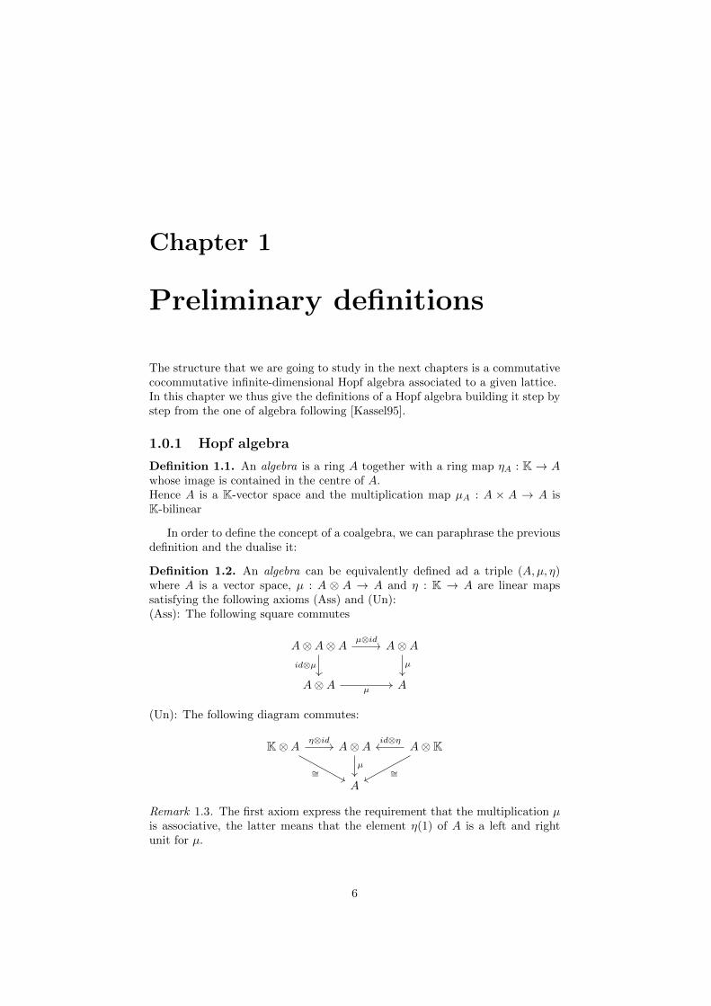
1.0.1 Hopf algebra
Definition 1.1. An algebra is a ring A together with a ring map ηA : K → Awhose image is contained in the centre of A.Hence A is a K-vector space and the multiplication map µA : A × A → A isK-bilinear
In order to define the concept of a coalgebra, we can paraphrase the previousdefinition and the dualise it:
Definition 1.2. An algebra can be equivalently defined ad a triple (A,µ, η)where A is a vector space, µ : A ⊗ A → A and η : K → A are linear mapssatisfying the following axioms (Ass) and (Un):(Ass): The following square commutes
A⊗A⊗A A⊗A
A⊗A A
µ⊗id
id⊗µ µ
µ
(Un): The following diagram commutes:
K⊗A A⊗A A⊗K
A
∼=
η⊗id
µ
id⊗η
∼=
Remark 1.3. The first axiom express the requirement that the multiplication µis associative, the latter means that the element η(1) of A is a left and rightunit for µ.
6
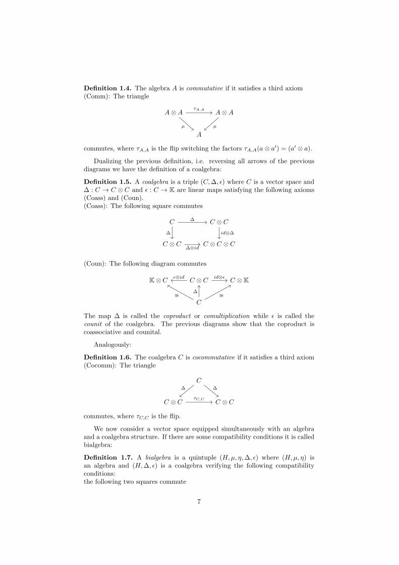
Definition 1.4. The algebra A is commutative if it satisfies a third axiom(Comm): The triangle
A⊗A A⊗A
A
τA,A
µ µ
commutes, where τA,A is the flip switching the factors τA,A(a⊗ a′) = (a′ ⊗ a).
Dualizing the previous definition, i.e. reversing all arrows of the previousdiagrams we have the definition of a coalgebra:
Definition 1.5. A coalgebra is a triple (C,∆, ε) where C is a vector space and∆ : C → C ⊗ C and ε : C → K are linear maps satisfying the following axioms(Coass) and (Coun).(Coass): The following square commutes
C C ⊗ C
C ⊗ C C ⊗ C ⊗ C
∆
∆ id⊗∆
∆⊗id
(Coun): The following diagram commutes
K⊗ C C ⊗ C C ⊗K
C
ε⊗id id⊗ε
∼=∆ ∼=
The map ∆ is called the coproduct or comultiplication while ε is called thecounit of the coalgebra. The previous diagrams show that the coproduct iscoassociative and counital.
Analogously:
Definition 1.6. The coalgebra C is cocommutative if it satisfies a third axiom(Cocomm): The triangle
C
C ⊗ C C ⊗ C
∆ ∆
τC,C
commutes, where τC,C is the flip.
We now consider a vector space equipped simultaneously with an algebraand a coalgebra structure. If there are some compatibility conditions it is calledbialgebra:
Definition 1.7. A bialgebra is a quintuple (H,µ, η,∆, ε) where (H,µ, η) isan algebra and (H,∆, ε) is a coalgebra verifying the following compatibilityconditions:the following two squares commute
7

H ⊗H H H ⊗H K⊗K
(H ⊗H)⊗ (H ⊗H) H ⊗H H K
µ
(id⊗τ⊗id)(∆⊗∆) ∆ µ
ε⊗ε
id
µ⊗µ ε
the following two diagrams commute
K H K H
K⊗K H ⊗H K
η
id ∆id
η
ε
η⊗η
We finally define the convolution of two linear maps:
Definition 1.8. Given (A,µ, η) algebra and (C,∆, ε) coalgebra, given f and gin Hom(C,A), we define the convolution f ?g as the composition of the followingmaps:
C C ⊗ C A⊗A A∆ f⊗g µ
We are now ready for the wanted definition:
Definition 1.9. A Hopf algebra is a bialgebra (H,µ, η,∆, ε) together with aK-linear map S : H → H such that
S ? id = id ? S = η ◦ ε
The endomorphism S is called antipode.
Remark 1.10. If the antipode exists, it is unique by definition.
Example 1.11. Given G group we can construct the group algebra K[G] asthe formal linear combinations of elements of G with coefficients in K.This happens to be a Hopf algebra (K[G], µ, η,∆, ε, S).Let us define the related maps:
∆ : K[G] −→ K[G]⊗K[G]
g 7−→ g ⊗ gε : K[G] −→ K
g 7−→ 1 ∀g ∈ Gη : K −→ K[G]
1 7−→ eG
µ : K[G]⊗K[G] −→ K[G]
g1 ⊗ g2 7−→ g1g2
S : K[G] −→ K[G]
g 7−→ g−1
8
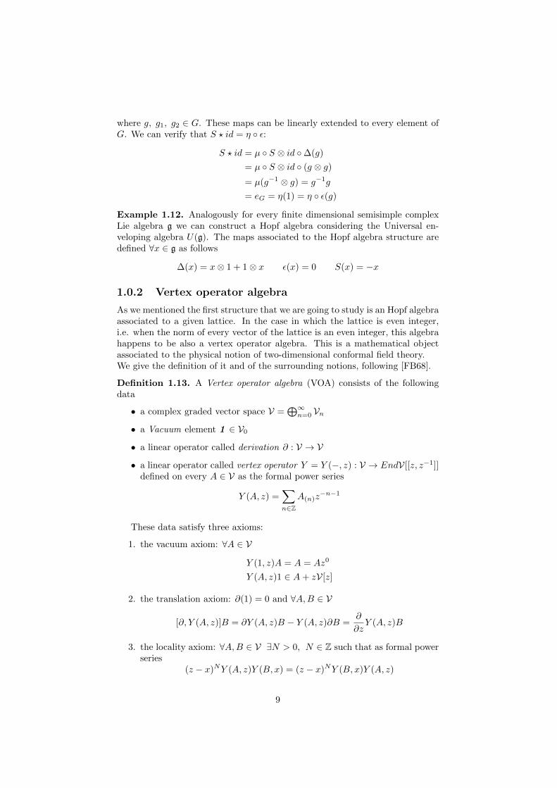
where g, g1, g2 ∈ G. These maps can be linearly extended to every element ofG. We can verify that S ? id = η ◦ ε:
S ? id = µ ◦ S ⊗ id ◦∆(g)
= µ ◦ S ⊗ id ◦ (g ⊗ g)
= µ(g−1 ⊗ g) = g−1g
= eG = η(1) = η ◦ ε(g)
Example 1.12. Analogously for every finite dimensional semisimple complexLie algebra g we can construct a Hopf algebra considering the Universal en-veloping algebra U(g). The maps associated to the Hopf algebra structure aredefined ∀x ∈ g as follows
∆(x) = x⊗ 1 + 1⊗ x ε(x) = 0 S(x) = −x
1.0.2 Vertex operator algebra
As we mentioned the first structure that we are going to study is an Hopf algebraassociated to a given lattice. In the case in which the lattice is even integer,i.e. when the norm of every vector of the lattice is an even integer, this algebrahappens to be also a vertex operator algebra. This is a mathematical objectassociated to the physical notion of two-dimensional conformal field theory.We give the definition of it and of the surrounding notions, following [FB68].
Definition 1.13. A Vertex operator algebra (VOA) consists of the followingdata
• a complex graded vector space V =⊕∞
n=0 Vn
• a Vacuum element 1 ∈ V0
• a linear operator called derivation ∂ : V → V
• a linear operator called vertex operator Y = Y (−, z) : V → EndV[[z, z−1]]defined on every A ∈ V as the formal power series
Y (A, z) =∑n∈Z
A(n)z−n−1
These data satisfy three axioms:
1. the vacuum axiom: ∀A ∈ V
Y (1, z)A = A = Az0
Y (A, z)1 ∈ A+ zV[z]
2. the translation axiom: ∂(1) = 0 and ∀A,B ∈ V
[∂, Y (A, z)]B = ∂Y (A, z)B − Y (A, z)∂B =∂
∂zY (A, z)B
3. the locality axiom: ∀A,B ∈ V ∃N > 0, N ∈ Z such that as formal powerseries
(z − x)NY (A, z)Y (B, x) = (z − x)NY (B, x)Y (A, z)
9

Remark 1.14. The locality axiom says that ∀A,B ∈ V, the formal power series intwo variables obtained by composing Y (A, z) and Y (B, x) in two possible waysare equal to each other, possibily after multiplying them with a large enoughpower of (z − x).
Definition 1.15. A vertex algebra homomorphism ρ between vertex algebras
ρ : (V, 1, ∂, Y )→ (V ′, 1′, ∂′, Y ′)
is a linear map V → V ′ mapping 1 to 1′, intertwining the translation operatorsand satisfying
ρ(Y (A, z)B) = Y (ρ(A), z)ρ(B).
Definition 1.16. A vertex subalgebra V ′ ⊂ V is a ∂-invariant subspace contain-ing the vacuum vector, and satisfying Y (A, z)B ∈ V ′((z)) for all A,B ∈ V ′.
For completeness’ sake, we here introduce the technical definition of a V-module. However we will just treat lattice vertex algebras: their representationtheory is fully known (described in 2.7) and we will just use the results on it.
Definition 1.17. Let (V, 1, ∂, Y ) be a vertex algebra. A vector space M iscalled a V-module if it id equipped with an operation YM : V → EndM [[z±1]]which assigns to each A ∈ V a field
YM (A, z) =∑n∈Z
AM(n)z−n−1
on M subject to the following axioms:
• YM (1, z) = IdM
• for all A,B ∈ V, C ∈M the three expressions
YM (A, z)YM (B,w)C ∈M((z))((w)),
YM (B,w)YM (A, z)C ∈M((w))((z)),
YM (YM (A, z − w)B,w)C ∈M((w))((z − w))
are the expansions, in their respective domains, of the same element of
M [[z, w]][z−1, w−1, (z − w)−1].
1.0.3 Super vector space
Lastly we give a third important definition that will be useful in Chapter 5 and6 when we will speak about the Symplectic Fermions.
Definition 1.18. A super vector space is a Z/2Z-graded vector space
V = V0 ⊕ V1
The elements of V0 are called even and the elements of V1 are called odd.The super dimension of a super vector space V is the pair (p, q) where dim(V0) =p and dim(V1) = q as ordinary vector spaces. We write dimV = p|q.
10
The super vector spaces form a braided tensor category where the morphismspreserve the Z/2Z grading. A braided tensor category is a tensor categoryequipped with a natural isomorphism called braiding, which switch two objectsin a tensor product. In this case for example the braiding is given by
x⊗ y → (−1)|x|+|y|y ⊗ x
We can then define a super algebra as an algebra in the category of super vectorspaces; explicitly:
Definition 1.19. A super algebra is a super vector space A together with abilinear multiplication morphism ηA : A⊗A → A such that
AiAj ⊆ Ai+j
where the indexes are read modulo 2.
Analogously it is possible to define a vertex operator superalgebra (VOSA).
11
Chapter 2
Setting
2.1 First steps in the VOA world
Let us consider a commutative cocommutative Hopf algebra V and let us con-struct on it some additional structure, defining:
• an Hopf pairing 〈 , 〉 : V ⊗ V −→ C[z, z−1] i.e. a z-dependent map suchthat the following relations hold:
〈ab, c〉 =⟨a, c(1)
⟩⟨b, c(2)
⟩〈a, bc〉 =
⟨a(1), b
⟩⟨a(2), c
⟩〈a, 1〉 = ε(a)
〈1, b〉 = ε(b)
where a, b, c ∈ V, ε is the Hopf algebra counit and a(1), a(2), c(1), c(2) arethe target terms of the Hopf algebra comultiplication ∆ where a sum isimplicit.
• a derivation or translator operator, ∂ : V → V such that:
∂.(ab) = (∂.a)b+ a(∂.b)
compatible with the Hopf pairing:
〈a, ∂.b〉 = − ∂
∂z〈a, b〉
〈∂.a, b〉 =∂
∂z〈a, b〉
From these data, under certain conditions (see [Lent17], [Lent07]), we can definea map, the vertex operator
Y : VΛ → EndVΛ[[z, z−1]],
a 7−→
b 7→∑k≥0
⟨a(1), b(1)
⟩· b(2) · z
k
k!∂k.a(2)
In turn it defines on V the structure of a local Vertex Algebra as proven in thequoted references.
12
Free particle in one dimension
As first example of such a Hopf algebra V we consider the free commutativealgebra generated by the formal symbols
∂φ, ∂2φ, ∂3φ, . . .
On V is naturally defined a N0-grading such that the N0-degree of ∂kφ is k.Every element is primitive as coalgebra element i.e.
∆∂1+kφ = 1⊗ ∂1+kφ+ ∂1+kφ⊗ 1
For every c ∈ C∗ we can construct a derivation and a Hopf pairing as follows:
∂.∂kφ = ∂k+1φ
〈∂φ, ∂φ〉 =c
z2
The following are some examples of the vertex operator Y applied to genericelements of V:
Y (1)∂hφ = ∂hφ
Y (∂hφ)1 =∑k
zk∂k
k!∂hφ =
∑k
zk
k!∂h+kφ
Y (∂φ)∂φ =c
z2+ ∂φY (∂φ)1
This V is ∀c ∈ C∗ the Heisenberg VOA defined in Chapter 2.1 of [FB68]. Froma physics perspective, V is as a vector space the space of states of a free particlein one dimension and the map Y represents an interaction between two statesto a third one.
Free particle in n-dimensional space or n free particles in one dimen-sion
We extend now the previous construction, considering the free commutativecocommutative Hopf algebra generated ∀α ∈ Rn by the formal symbols:
∂φα, ∂2φα, ∂
3φα, . . .
with the following relation:
∂1+kφaα+bβ = a∂1+kφα + b∂1+kφβ
where a, b ∈ R and α, β ∈ Rn. Because of this linear combination it actuallysuffices to take as generators the elements
∂φα1, . . . , ∂φαn
for any fixed basis {α1, . . . αn} of Rn. This Hopf algebra can now be endowedas before with a derivation and an Hopf pairing. In particular we have:
〈∂φα, ∂φβ〉 =(α, β)
z2
Physically the system describes a free particle in a n-dimensional space, orequivalently, n particles in one dimension.
13
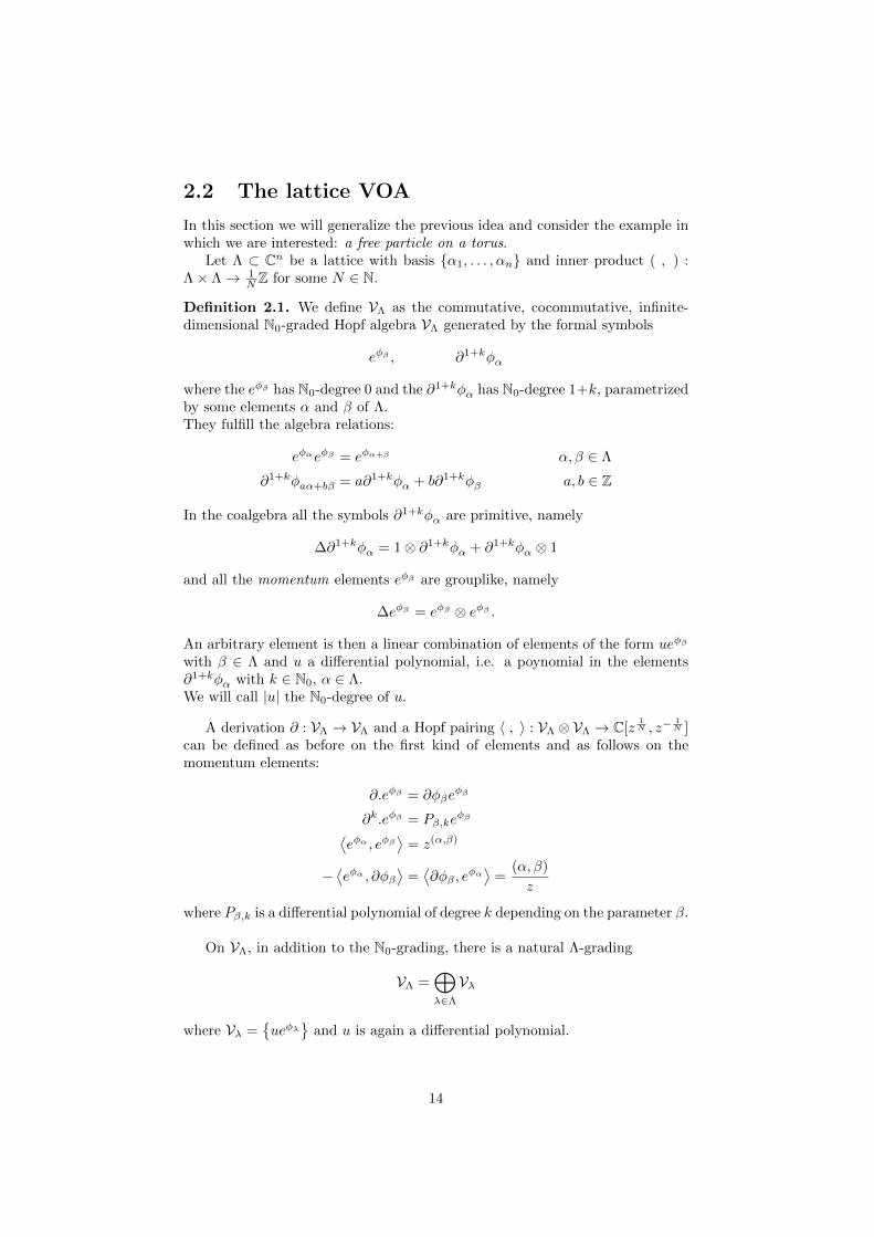
2.2 The lattice VOA
In this section we will generalize the previous idea and consider the example inwhich we are interested: a free particle on a torus.
Let Λ ⊂ Cn be a lattice with basis {α1, . . . , αn} and inner product ( , ) :Λ× Λ→ 1
NZ for some N ∈ N.
Definition 2.1. We define VΛ as the commutative, cocommutative, infinite-dimensional N0-graded Hopf algebra VΛ generated by the formal symbols
eφβ , ∂1+kφα
where the eφβ has N0-degree 0 and the ∂1+kφα has N0-degree 1+k, parametrizedby some elements α and β of Λ.They fulfill the algebra relations:
eφαeφβ = eφα+β α, β ∈ Λ
∂1+kφaα+bβ = a∂1+kφα + b∂1+kφβ a, b ∈ Z
In the coalgebra all the symbols ∂1+kφα are primitive, namely
∆∂1+kφα = 1⊗ ∂1+kφα + ∂1+kφα ⊗ 1
and all the momentum elements eφβ are grouplike, namely
∆eφβ = eφβ ⊗ eφβ .
An arbitrary element is then a linear combination of elements of the form ueφβ
with β ∈ Λ and u a differential polynomial, i.e. a poynomial in the elements∂1+kφα with k ∈ N0, α ∈ Λ.We will call |u| the N0-degree of u.
A derivation ∂ : VΛ → VΛ and a Hopf pairing 〈 , 〉 : VΛ ⊗ VΛ → C[z1N , z−
1N ]
can be defined as before on the first kind of elements and as follows on themomentum elements:
∂.eφβ = ∂φβeφβ
∂k.eφβ = Pβ,keφβ⟨
eφα , eφβ⟩
= z(α,β)
−⟨eφα , ∂φβ
⟩=⟨∂φβ , e
φα⟩
=(α, β)
z
where Pβ,k is a differential polynomial of degree k depending on the parameter β.
On VΛ, in addition to the N0-grading, there is a natural Λ-grading
VΛ =⊕λ∈Λ
Vλ
where Vλ ={ueφλ
}and u is again a differential polynomial.
14
Definition 2.2. The Vertex algebra operator Y is defined as
Y : VΛ → EndVΛ[[z1N , z−
1N ]],
a 7−→
b 7→∑k≥0
⟨a(1), b(1)
⟩· b(2) · z
k
k!∂k.a(2)
Depending on the lattice Λ, this algebra VΛ happens to be a more complex
algebraic object.
Definition 2.3. A lattice Λ is called even integer lattice if the norm of everyvector is an even integer. In particular this implies that the inner product hasalways integer values.A lattice Λ is called an odd integer lattice if the norm of every vector is aninteger but not necessarily even.A lattice Λ is called a not integer or fractional lattice if there exist non integernorms.
Theorem 2.4. • [FB68] If Λ is an even integer lattice then (VΛ, Y ) is alattice vertex algebra (VOA), i.e. a vertex algebra whose elements areparametrized by the one of the lattice Λ.
• [FB68] If Λ is an odd integer lattice then (VΛ, Y ) is a lattice super vertex al-gebra (VOSA), i.e. a super vertex algebra whose elements are parametrizedby the one of the lattice Λ.
Remark 2.5. If Λ is not integer, i.e. is fractional, then the locality in VΛ isreplaced by other relations (see [Lent17] ) and we can still speak about it assome generalized lattice VOA.
We now consider the dual lattice Λ∗ = {λ ∈ C| (λ, α) ∈ Z ∀α ∈ Λ}. Thefollowing result, shown in Chapter 5 of [FB68], gives us informations about therepresentation category VΛ-Rep of a lattice VOA VΛ.
Remark 2.6. It is possible to have an action of VΛ on VΛ∗ through the vertexoperator Y because the inclusion Λ ⊂ Λ∗ implies
Y : VΛ × VΛ∗ → VΛ∗
and from the definition of the dual lattice we have only integer z-powers. Ex-plicitly, if α ∈ Λ and λ ∈ Λ∗ then α+ λ ∈ Λ∗ and (α, λ) ∈ Z. Thus
Y (eφα)eφλ = 〈z, z−1, φ1+k〉 eφα+λ ∈ VΛ∗
Theorem 2.7. Let Λ be a even integer lattice, then VΛ-Rep is a category equiv-alent to the category of (Λ∗/Λ)-Vect i.e. the vector spaces graded by the abeliangroup (Λ∗/Λ). We can decompose the module
VΛ∗ =⊕
[λ]∈Λ∗/Λ
V[λ]
i.e. as direct sum of simple modules. We call VΛ = V[0] the vacuum module.
15
Remark 2.8. The equivalence of Theorem 2.7 is as abelian categories. Moreover,asking some finiteness conditions on VΛ, its representation category becomes amodular tensor category; then adding a braiding of the form eiπ(λ,λ′) on theright side the equivalence is also as modular tensor categories.
Remark 2.9. The equivalence as abelian categories implies, in particular, thatthe simple objects of the two categories corresponds and thus their numbercoincides. Therefore we have as many VΛ-simple modules in VΛ-Rep as one di-mensional vector spaces in the category of (Λ∗/Λ)-graded vector spaces. Sincein the latter, we have one dimensional vector spaces for every layer, we have ex-actly |Λ∗/Λ| one dimensional vector spaces and thus, irreducible representationsof VΛ.
2.3 Screening operators
Once the vertex operator Y is defined, we can produce linear endomorphismsof VΛ as follows:
Definition 2.10. For a given element a ∈ VΛ and m ∈ 1NZ we can consider the
zm-term ofY (a)b =
∑m
Y (a)mzmb
with b ∈ VΛ, and thus produce an endomorphism: the mode operator
Y (a)m : VΛ → VΛ b 7−→∑k≥0
⟨a(1), b(1)
⟩−k+m
b(2) 1
k!∂k.a(2)
where 〈a, b〉n denotes the zn-coefficient.
From this we can define also the so-called ResY -operator, an operator thatfor every b give us an endomorphism of VΛ:
Definition 2.11. Given a ∈ Vα, b ∈ Vβ and m := (α, β)
ResY (a) : b 7−→ Res(Y (a)b)
Res(Y (a)b) :=
Y (a)−1 if m ∈ Ze2πim−1
2πi
∑k∈Z
1m+k+1Y (a)m+k if m /∈ Z
where the residue is defined as a formal residue of fractional polynomials andgeometrically is the integral along the unique lift of a circle with given radiusto the multivalued covering on which the polynomial with fractional exponentsis defined.
In the integer case this endomorphism has a derivational property thanks tothe OPE associativity [Thiel94], [FB68]:
Y (a)−1 (Y (b)mc) = Y (Y (a)−1b)mc± Y (b)m (Y (a)−1c) (2.1)
Using the residue we arrive to define some interesting maps on the lattice VOAVΛ and its modules i.e. the screening charge operators.
16
Definition 2.12. For α ∈ Λ∗ we define the screening charge operator Zα as
Zαv := ResY (eφα)v
By the given definition, if (α, β) ∈ Z it simplifies to
Zαueφβ =
∑k≥0
〈eφα , u(1)〉−k−1−(α,β)u(2)eφβ
1
k!∂k.eφα (2.2)
Remark 2.13. We notice that the operators shift the Λ-grading
Zα : Vλ → Vλ+α
Moreover in the case of α ∈ Λ they fix the VΛ-modules i.e.
Zα : V[λ] → V[λ]
where [λ] ∈ Λ∗/Λ.
The screening operators are an old construction in CFT. In the case of non-integral lattice we have however a new result by [Lent17] that gives us relationsof screenings. This result follows in the same paper from the study of thecomplicated structures of Nichols algebra.For our purposes it is not necessarily to define such structures but it is interestingto state the Theorem because its consequences (displayed in section 2.6) are oneof the motivations of this work.
Theorem 2.14. [Lentner17] Let Λ be a positive-definite lattice and {α1, . . . , αn}be a fixed basis that fulfils |αi| ≤ 1. Then the endomorphisms Zαi := ResY (eφαi )on the fractional lattice VOA VΛ constitute an action of the diagonal Nicholsalgebra generated by the Zαi with braiding matrix
qij = eπi(αi,αj).
The theorem proves that the screening operators associated to a small enoughlattice obey Nichols algebra relations.
Corollary 2.15. As consequences of the theorem we have:
• if (α, α) is an odd integer ⇒ (Zα)2 = 0
• if (α, β) is an even integer ⇒ Zα and Zβ commute.
What we will do next is to find Λ root lattice of some Lie algebra such thatqij is the braiding of a quantum group. But first we want to introduce thenotion of Virasoro Algebra and understand how does it act on our VOA.
2.4 Virasoro action
Definition 2.16. The Witt algebra is a Lie algebra generated by the vectorfields
Ln := −zn+1 ∂
∂z
with n ∈ Z. The Lie bracket of two vector fields is given by
[Lm, Ln] = (m− n)Lm+n
17
This is the Lie algebra of the group of diffeomorphisms of the circle.
Definition 2.17. The Virasoro Algebra V irc is the non-trivial central extensionof the Witt Lie algebra. It is generated by the central charge C = c1, c ∈ C, andthe operators Ln indexed by an integer n ∈ Z and that fulfil the commutationrelations
[Lm, Ln] = (m− n)Lm+n +C
12(m3 −m)δm+n,0
[Ln, C] = 0 ∀n ∈ Z.
Definition 2.18. A vertex algebra V is called conformal, of central chargec ∈ C, if there is a non-zero conformal vector ω ∈ V2 such that the Y (ω)−2−n ofthe corresponding vertex operator satisfy the defining relations of the Virasoroalgebra with central charge c and in addition we have Y (ω)−1 = ∂, Y (ω)0|Vn =nId.
On our lattice VOA VΛ we have the following result by [FF88] which inparticular tell us that VΛ is conformal:
Theorem 2.19. If we choose an Energy-Stress tensor in VΛ
T =1
2
∑i
∂φαi∂φαi∗ +∑i
Qi∂2φαi ,
depending on an arbitrary vector Q = (Q1, . . . , Qn) ∈ spanC〈α1, . . . , αn〉 andindependent of the choice of a dual basis (αi, αj
∗) = δij, then Ln := Y (T )−2−nconstitute an action of the Virasoro algebra V irc with central charge c = rank−12(Q,Q) on VΛ.
Remark 2.20. Since T ∈ VΛ, in this way we automatically obtain a Virasoroaction also on all the vertex modules of VΛ.
Remark 2.21. The action of V irc on VΛ is an action on the vector space and onevery module that is compatible with the VOA structure (defined in Chapter1).
Lemma 2.22. For the defined T , fixed a value of Q, the action of the L0 andL−1 elements of V irc on a generic element ueφβ of the VOA VΛ is given by:
L−1ueφβ = ∂.(ueφβ )
L0ueφβ =
((β, β)
2− (β,Q) + |u|
)ueφβ
The L0 eigenvalues are called conformal dimensions.
Proof. Here we just verify the action of L−1.
L−1ueφβ = Y (
1
2
∑i
∂φαi∂φαi∗ +∑i
Qi∂2φαi)
−1
ueφβ =
=1
2
∑i
Y (∂φαi∂φαi∗)−1ueφβ +
∑i
QiY (∂2φαi)−1ueφβ
18
The co-multiplications of the T summands are:
∆(∂φαi∂φαi∗) = ∆(∂φαi)∆(∂φαi∗)
= 1⊗ ∂φαi∂φαi∗ + 2∂φαi ⊗ ∂φαi∗ + ∂φαi∂φαi∗ ⊗ 1
∆(∂2φαi) = 1⊗ ∂2φαi + ∂2φαi ⊗ 1
Now we write temporarily v := ueφβ and define
A := Y (∂φαi∂φαi∗)v
B := Y (∂2φαi)v
and we explicitly compute them:
A = 〈1, v(1)〉v(2)∑k
zk∂k
k!(∂φαi∂φαi∗) + 2〈∂φαi , v(1)〉v(2)
∑k
zk∂k
k!∂φαi∗
+ 〈∂φαi∂φαi∗, v(1)〉v(2)∑k
zk∂k
k!1
= 0 + 2∑k
〈∂φαi , v(1)〉nv(2)zk+n ∂k+1φαi∗k!
+ 〈∂φαi∂φαi∗, v(1)〉nv(2)zn
B = 〈1, v(1)〉v(2)∑k
zk∂k
k!∂2φαi + 〈∂2φαi , v
(1)〉v(2)∑k
zk∂k
k!1
= v∑k
zk
k!∂k+2φαi + 〈∂2φαi , v
(1)〉nv(2)zn.
Going back to the first equation and noticing that the term B vanishes, weobtain:
L−1ueφβ =
1
2
∑i
(2∑k
〈∂φαi , u(1)eφβ 〉−k−1u(2)eφβ
∂k+1φαi∗k!
+ 〈∂φαi∂φαi∗, u(1)eφβ 〉−1u(2)eφβ
)+∑i
Qi〈∂2φαi , u(1)eφβ 〉−1u
(2)eφβ
The last two terms vanish:
1.
〈∂φαi∂φαi∗, u(1)eφβ 〉 = 〈1, eφβ 〉〈∂φαi∂φαi∗, u(1)〉+ 2〈∂φαi , eφβ 〉〈∂φαi∗, u(1)〉+ 〈∂φαi∂φαi∗, eφβ 〉〈1, u(1)〉
=
{〈∂φαi∂φαi∗, eφβ 〉 if u(1) = 1
2〈∂φαi , eφβ 〉〈∂φαi∗, u(1)〉 if u(1) 6= 1
and both cases give some power of z with exponential lower than −1.
2.
〈∂2φαi , u(1)eφβ 〉 = ∂〈∂φαi , u(1)eφβ 〉 = ∂
[〈∂φαi , u(1)〉〈1, eφβ 〉+ 〈1, u(1)〉〈∂φαi , eφβ 〉
]=
{∂〈∂φαi , eφβ 〉 if u(1) = 1
∂〈∂φαi , u(1)〉 if u(1) 6= 1
and again both cases give some power of z lower than −1.
19
Hence we obtain
L−1ueφβ =
∑i
∑k
〈∂φαi , u(1)eφβ 〉−k−1u(2)eφβ
∂k+1φαi∗k!
=∑i
∑k1+k2=−k−1
(〈∂φαi , u(1)〉k1
〈1, eφβ 〉k2+ 〈1, u(1)〉k1
〈∂φαi , eφβ 〉k2
)u(2)eφβ
∂k+1φαi∗k!
Now we split it again in two cases
• If u(1) = 1 then we just have the second summand
∑i
∑k
〈∂φαi , eφβ 〉−k−1ueφβ∂k+1φαi∗
k!=∑i
(αi, β)ueφβ∂φαi∗
=∑i
(αi, β)ueφβ ~α∗i · ∂~φ =∑i
ueφβ ~αi · ~β · ~α∗i · ∂~φ
= ueφβ ~β · ∂~φ = ueφβ∂φβ = u(∂.eφβ )
where we had highlighted the vector nature of ∂φ and the elements α ofthe n-dimensional lattice Λ.
• If u(1) 6= 1 then we just have the first summand
∑i
∑k
〈∂φαi , u(1)〉−k−1u(2)eφβ
∂k+1φαi∗k!
In this case the only possible u(1) such that the Hopf pairing is non-zerois u(1) = ∂n+1φγ . In particular u(2) = 1. We have now
〈∂φαi , ∂n+1φγ〉 = −∂.〈∂φαi , ∂nφγ〉= (−1)2∂2.〈∂φαi , ∂n−1φγ〉= (−1)n∂n.〈∂φαi , ∂φγ〉= (−1)n∂n(αi, γ)z−2
= (−1)2n(n+ 1)!z−(n+2)(αi, γ)
Thus, the only term not equal to zero is for k = n+ 1. We obtain:∑i
1
(n+ 1)!(n+ 1)!(αi, γ)eφβ∂n+2φαi∗ = ∂n+2φγe
φβ = ∂.(∂n+1φγ)eφβ
Putting together these two cases we have:
L−1ueφβ = u(∂.eφβ ) + (∂.u)eφβ
⇒ L−1ueφβ = ∂.(ueφβ )
We now qualitatively describe the modules of V irc and its action on them.
20
• The modules of V irc are given by the Λ-grading layers Vλ.Indeed we have that every operator Ln acts on an element ueφβ increasing(if n < 0) or decreasing (if n > 0) its N0-degree of n, but doesn’t shift theΛ-grading.For example the L−1 operator acts as a derivation, i.e. as follows:
∂.eφλ := ∂φλeφλ
∂.∂kφα := ∂1+kφα
and more generally it increases the degree of ueφλ by 1, but maintains thestructure Polynomial · eφλ .
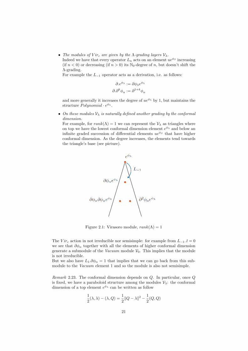
• On these modules Vλ is naturally defined another grading by the conformaldimension.For example, for rank(Λ) = 1 we can represent the Vλ as triangles whereon top we have the lowest conformal dimension element eφλ and below aninfinite graded succession of differential elements ueφβ that have higherconformal dimension. As the degree increases, the elements tend towardsthe triangle’s base (see picture).
Figure 2.1: Virasoro module, rank(Λ) = 1
The V irc action in not irreducible nor semisimple: for example from L−1.1 = 0we see that ∂φα together with all the elements of higher conformal dimensiongenerate a submodule of the Vacuum module V0. This implies that the moduleis not irreducible.But we also have L1.∂φα = 1 that implies that we can go back from this sub-module to the Vacuum element 1 and so the module is also not semisimple.
Remark 2.23. The conformal dimension depends on Q. In particular, once Qis fixed, we have a paraboloid structure among the modules Vλ: the conformaldimension of a top element eφλ can be written as follow
1
2(λ, λ)− (λ,Q) =
1
2‖Q− λ‖2 − 1
2(Q,Q)
21
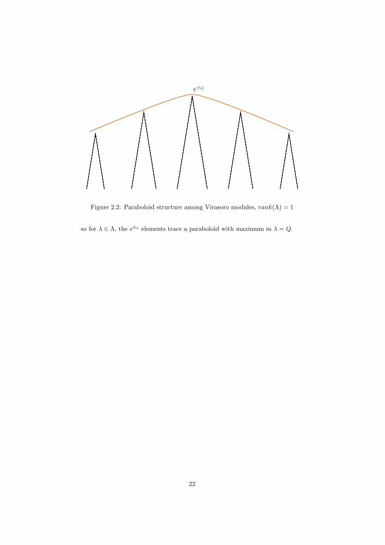
Figure 2.2: Paraboloid structure among Virasoro modules, rank(Λ) = 1
so for λ ∈ Λ, the eφλ elements trace a paraboloid with maximum in λ = Q.
22
2.5 Rescaled root lattices
Let g be a complex finite dimensional semisimple Lie algebra. Denote by:
• ΛR its root lattice with basis {α1, . . . , αrank}
• ΛW its weight lattice i.e. the lattice spanned by the fundamental weights{λ1, . . . , λrank} such that (λi, αj) = djδij = 1
2 (αj , αj)δij
• ΛR∨ its coroot lattice with basis {α1
∨, . . . , αrank∨} where αi
∨ := αi2
(αi,αi)
Let ` = 2p be an even natural number divisible by all (αj , αj).
We rescale the root lattice ΛR.
Definition 2.24. We call short screening lattice Λ := 1√pΛR with basis the
short screening momenta{α1 := − α1√
p, . . . , αrank
:= −αrank√p
}.
We now consider the (generalized) lattice VOA VΛ . By Lemma 2.22 weknow that for every value of Q there is a Virasoro action on the algebra. Thus welook for the unique value of Q such that the conformal dimension of the elementseφαi , that we will denote by hQ(αi
), is equal to 1. We will understand laterwhy this is convenient.
Lemma 2.25. The unique Q such that hQ(αi) = 1 is given by Q = (p · ρg∨−
ρg)/√p, where we define ρg as the half sum of all positive roots, and ρg
∨ theanalogous for the dual root system.
Proof. To prove it we have to show that
1
2(αi, αi
)− (αi, Q) = 1
So, let us compute the first term:
1
2(− αi√
p,− αi√
p)− (− αi√
p, (p · ρg∨ − ρg)
1√p
)
=1
2p(αi, αi) +
1
p(αi, p · ρg∨)− 1
p(αi, ρg)
=1
2p(αi, αi) + (αi, ρg
∨)− 1
p
(αi, αi)
2
= (αi, ρg∨) =
(αi, αi)
2(αi∨, ρg
∨)
=(αi, αi)
2
(αi∨, αi
∨)
2= 1
where we used that αi∨ = αi
2(αi,αi)
and (αi, ρg) = (αi,αi)2 .
Lemma 2.26. Fixed Q = (p · ρg∨ − ρg)/√p as above, another combination of
elements of ΛR, β, such that hQ(β) = 1 is given by β := αi∨√p
23
Proof. Let’s compute hQ(β)
1
2(αi∨√p, αi∨
√p)− (αi
∨√p, (p · ρg∨ − ρg)/√p)
=p
2(αi∨, αi
∨)− (αi∨, p · ρg∨) + (αi
∨, ρg)
=p
2(αi∨, αi
∨)− p
2(αi∨, αi
∨) +2
(αi, αi)(αi, ρg) = 1
Hence, once the lattice ΛR is rescaled to Λ, the choice of such a Q givesdirectly a second lattice spanned by roots β such that hQ(β) = 1.
Definition 2.27. The long screening lattice is Λ⊕ :=√pΛR
∨ with basis thelong screening momenta
{α1⊕ := α∨1
√p, . . . , αrank
⊕ := α∨rank√p}.
We consider lastly a third bigger lattice (Λ⊕)∗
defined as the dual lattice ofΛ⊕ namely as the one spanned by some λ1
∗, . . . λrank∗ such that (λi
∗, αj⊕) =
δij .
Lemma 2.28. This lattice happens to be equal to the rescaled weight lattice:
(Λ⊕)∗ =1√p
ΛW
Proof. The equality can be easily proved:
(λi∗, αj
⊕) = (1√pλi,√pαj∨) = (
1√pλi,√pαj
2
(αj , αj)) =
2
(αj , αj)(λi, αj) = δij
The inclusion relationships among these three lattices is as follows:
Λ⊕ ⊂ Λ ⊂ (Λ⊕)∗
Remark 2.29. The choice of l = 2p to be divisible by all (αj , αj) implies thatΛ⊕ is integral. This in turn implies that VΛ⊕ is a lattice VOA.Instead we will talk about generalized lattice VOA in the case of VΛ and V(Λ⊕)∗
Corollary 2.30. The number of irreducible representations of VΛ⊕ is, by The-orem 2.7 equal to |(Λ⊕)
∗/Λ⊕|. To compute it, it is in general helpful to use the
intermediate lattice Λ as follows
|(Λ⊕)∗/Λ⊕| = |(Λ⊕)
∗/Λ| · |(Λ)/Λ⊕|
= | 1√p
ΛW /1√p
ΛR| · |1√p
ΛR/√pΛ∨R|
= |ΛW /ΛR| ·
∣∣∣∣∣⊕αi
(1√pαiZ/
√p
2
(αi, αi)αiZ
)∣∣∣∣∣= |ΛW /ΛR| ·
rank∏i=1
`
(αi, αi)
where the order of ΛW /ΛR is the determinant of the Cartan matrix.
24
2.6 Application of results
We will now apply the results displayed in section 2.2, 2.3, 2.4 to the latticeVOAs associated to the three lattices Λ,Λ⊕, (Λ⊕)
∗.
Let VΛ⊕ be the lattice VOA associated to the lattice Λ⊕. We know that itssimple vertex algebra modules are V[λ] parametrized by (Λ⊕)
∗/Λ⊕ and we can
decompose
V(Λ⊕)∗ =⊕
[λ]∈(Λ⊕)∗/(Λ⊕)
V[λ].
Moreover, as said in Remark 2.20, the action of V irc on VΛ⊕ given by the vertexoperator passes automatically on all the VΛ⊕ -modules V[λ]. Any VΛ⊕ -moduleV[λ] decompose as Virasoro module into its Λ-grading layers:
V[λ] =⊕λ∈[λ]
Vλ (2.3)
Theorem 2.14 applied to the lattice Λ = Λ implies:
Corollary 2.31. For those roots αi such that (αi
, αi) ≤ 1, i.e. (αi, αi) ≤ p,
the short screening operators Zαi constitute a representation on V(Λ⊕)∗ of theNichols algebra for braiding
qij = eπi(− αi√
p ,−αj√p )
= eπip (αi,αj) = q(αi,αj)
with q := e2πi` a `-th root of unity. This is precisely the representation of the
postive part of the small quantum group uq(g)+.
On the other hand a classical result in [TF09] for g simply-laced says:
Corollary 2.32. The long screening operators Zαi⊕ constitute a representation
of the negative part of the enveloping algebra of g∨: U(g∨)−
Remark 2.33. A conjecture in [Lent17] affirms it for the general non simply-lacedcase.
We chose the Virasoro action parametrized by Q such that the followingconformal dimensions are
hQ(αi) = hQ(αi
⊕) = 1
Thanks to the usual OPE associativity (equation 2.1) for the integer operatorsZαi⊕ this implies:
Corollary 2.34. The long screening operators Zαi⊕ commute with the Virasoroaction, i.e. that they are Virasoro homomorphisms.
In [Lent17] it is proven that this commutativity relation holds in a weakerform also for the short screening case thanks to Nichols algebra relations:
25
Corollary 2.35. There exist a h ∈ N depending on the modules V[λ] such
that the Weyl reflections (Zαi)h
around the vector Q, called Steinberg point,commute with the Virasoro action, i.e. are Virasoro homomorphisms.
For example, in the vacuum module V[0] = VΛ⊕ we have h = 1. So on thismodule all (Zαi) are Virasoro homomorphisms. Finally, from the definition ofscreening operators we have
Corollary 2.36. The Zαi⊕ ’s preserve the VΛ⊕-modules and the Zαi ’s preservethe Λ cosets.
2.7 Example A1
Let us now focus on the easiest example of a Lie algebra g of type A1 alreadytreated in [FGST06a], [TW13], [NT11].We will compute the three lattices Λ, Λ⊕ and (Λ⊕)∗ as defined in section 2.5.We will then consider the lattice VOA VΛ⊕ and obtain its simple modules.
Consider thus g = sl2 and its root lattice ΛR = αZ with α simple root suchthat (α, α) = 2. For the moment we assume ` = 2p an arbitrary even number.
• We start as before by rescaling the root lattice to the short screeninglattice
Λ = αZ = − α√pZ.
with short screening momentum α = − α√p .
• To compute Q as in Lemma 2.25, we first notice that in this case α∨ =α 2
(α,α) = α and
ρg = ρg∨ =
1
2α
so we easily arrive to
Q =1√p
(pρg∨ − ρg) =
1
2√p
(p · α− α) =1
2
(p− 1)√p
α = −p− 1
2α
Remark 2.37. In this case, since there is just one simple root we cancompute Q also directly. From the general ansatz we know indeed thatQ = kα with k ∈ C, is the only one such that the property hQ(αi
) = 1holds. This implies that it has to be:
1
2(− α√p,− α√p
)− (− α√p, kα) = 1
1
2p(α, α) +
k√p
(α, α) = 1
⇒ k =1
2
(p− 1)√p
and then Q = 12
(p−1)√p α, as claimed.
26
• Consider then the long screening lattice Λ⊕ = Zα⊕ found as before re-quiring hQ(α⊕) = 1. From Lemma 2.26 we obtain:
α⊕ = α√p Λ⊕ = α
√p Z
again because α∨ = α 2(α,α) = α.
• To have the third lattice we have to compute the fundamental weight i.e.the λ = kα such that (λ, α) = 1
2 (α, α) = 1. Immediately we arrive tok = 1
2 and so:
(Λ⊕)∗ =1√p
ΛW =α
2√pZ
• Now we can compute the number of representations of VΛ⊕ :∣∣(Λ⊕)∗/Λ⊕∣∣ =
∣∣(Λ⊕)∗/Λ∣∣ · ∣∣Λ/Λ⊕∣∣ =
=
∣∣∣∣ 1√p
ΛW /1√p
ΛR
∣∣∣∣ · ∣∣∣∣ 1√p
ΛR/√pΛR
∨∣∣∣∣ =
= |ΛW /ΛR| ·∣∣∣∣ 1√p
ΛR/√pΛR
∨∣∣∣∣ =
= 2
∣∣∣∣− 1√pαZ/√pαZ
∣∣∣∣ = 2 |Zp| = 2p
• Explicitly these 2p representations are given by the cosets with represen-tatives:
(Λ⊕)∗/Λ⊕ =
{[kα
2√p
] : k = 0, 1, . . . , 2p− 1
}that fall into two Λ-cosets
0 + Λ/Λ⊕ = { kα2√p, k even} α
2√p
+ Λ/Λ⊕ = { kα2√p, k odd}.
The representations are thus V[ kα2√p ], with k = 0, 1, . . . , 2p− 1.
27
Chapter 3
The W subspace
We now want to use the short screenings to construct a subspace W of thelattice VOA VΛ⊕ following the so called free-field realization.
The subject of study is
W := VΛ⊕ ∩⋂i
kerZαi .
Remark 3.1. The space W is a sub vertex algebra of VΛ⊕ due to OPE associa-tivity (equation 2.1).
On this space a conjecture has been formulated successively by several au-thors [FF88], [FFHST02], [TF09], [FGST06a], [AM08]:
Conjecture 3.2. 1. W is a vertex subalgebra with an action of the Lie algebrag∨ via the long screenings.
2. It is a Logarithmic conformal field theory (LCFT) i.e. a VOA with finitenonsemisimple representation theory.
3. Its Representation category is equivalent to the one of the respective smallquantum group uq(g) at a root of unity q of order ` = 2p .
Remark 3.3. Saying that a LCFT is a VOA with (nonsemisimple) finite repre-sentation theory means that the Rep category is a finite tensor category in thesense of [EO03].
The construction of such aW is interesting because of the third point of theconjecture and in its own right, since few logarithmic CFTs are known: mostimportantly the triplet algebra Wp, which is exactly the one we will constructthrough free field realization in the A1 case, and the even part of n pairs ofsymplectic fermions that we will study later on.
In the next section we will go deeper in the study of the VΛ⊕ -modules andwe will look at this new space W and at its representations in the particularcase A1, ` = 4.
28
3.1 A1, ` = 4
3.1.1 Lattices
Let us consider again the previous example, specialized to ` = 2p = 4. For thisvalue of ` we have:
• Q = α2√
2
• Λ = Z α√2, α = − α√
2
• Λ⊕ = Zα√
2 α⊕ =√
2α,
• (Λ⊕)∗
= Z α2√
2λ∗ = α
2√
2
• the number of simple representations of V⊕Λ is now 4 and they are givenby the classes of (Λ⊕)∗/Λ⊕, [ kα
2√
2] for k = 0, 1, 2, 3; explicitly:
V[0], V[ α2√
2], V[ 2α
2√
2], V[ 3α
2√
2]
To simplify what follows we give informal names to them:Blue (or Vacuum), Steinberg, Green and Facet module.
3.1.2 Groundstates
We now introduce the notion of groundstates elements. These give us infor-mation about the modules and are the elements on which we will apply thescreening operators in the next section.
Definition 3.4. The space of groundstates is the L0-eigenspace associated withthe minimal eigenvalue, i.e. the minimal conformal dimension.
Remark 3.5. For each module V[ kα2√
2] of VΛ⊕ , a preferred basis for this space are
the elements eφλ with λ ∈ [ kα2√
2] vector with minimal distance to Q.
Definition 3.6. In particular in this work we will understand under the nameof groundstates elements exactly the elements eφλ with λ of minimal distanceto Q.
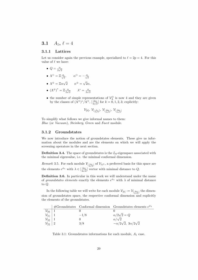
In the following table we will write for each module V[k] := V[ kα2√
2] the dimen-
sion of groundstates space, the respective conformal dimension and explicitlythe elements of the groundstates.
#Groundstates Conformal dimension Groundstates elements eφλ
V[0] 1 0 0
V[1] 1 −1/8 α/2√
2 = Q
V[2] 1 0 α/√
2
V[3] 2 3/8 −α/2√
2, 3α/2√
2
Table 3.1: Groundstates informations for each module, A1 case.
29
3.1.3 Screening operators
We now focus on the screening operators and on their action. From the Corol-lary 2.34 and 2.35 of Section 2.6 we know that the long screening operatorsand some power of the short screening operators are Vir -homomorphisms. Inparticular on the Blue and Green modules this power is equal to 1, i.e. onthem the short screening operators are really Vir -homomorphisms.
We will now explicitly apply the screening operators short Z−α/√
2 and long Zα√
2
to our modules to see how they act. Since ∀β ∈ [0], [ 2α2√
2] we have (− α√
2, β) ∈ Z
we can use formula 2.2 of Definition 2.12.
Remark 3.7. We notice that, from the consequences of Theorem 2.14, since(−α/
√2,−α/
√2) = 1 is an odd integer, then (Z−α/
√2)
2= 0 holds.
We start applying the short screening operator to the first two layers of Blueand Green modules:
1. The short screening operator applied to the Blue groundstates element(i.e. with conformal dimension equal to 0) give us the result:Z−α/
√2(e0) = Z−α/
√2(1) = 0
2. The short screening operator applied to the second layer (i.e. with con-formal dimension equal to 1) of the Blue module gives us the results:
Z−α/√
2(∂φα/√
2) =
=∑k
⟨eφ− α√
2 , ∂φα/√
2
⟩−k−1
1
k!∂ke
φ− α√2 +
∑k
⟨eφ− α√
2 , 1⟩−k−1
∂φα/√
2
1
k!∂ke
φ− α√2
=⟨eφ− α√
2 , ∂φα/√
2
⟩−1eφ− α√
2 + 0
= −(α√2,− α√
2)eφ− α√
2 = eφ− α√
2
Z−α/√
2(eφα√
2) =
=∑k
⟨eφ− α√
2 , 1⟩−k−1+2
eφα√
21
k!∂ke
φ− α√2 = ∂φ−α/
√2eφ α√
2
In the first equation the first term gives a nonzero result if and only ifk = 0; the second term vanishes because it could be non zero just fork = −1 but k > 0.In the second equation k must be equal to 1.
3. The short screening operator applied to the Green groundstates element(i.e. with conformal dimension equal to 0) gives us the result:
Z−α/√
2(eφ α√
2 ) =∑k
⟨eφ− α√
2 , 1⟩−k−1+1
eφ α√
21
k!∂ke
φ− α√2 =
=⟨eφ− α√
2 , 1⟩
0eφ α√
2 = e0 = 1
since the only term non equal to zero is for k = 0.
30
4. The short screening operator applied to the second layer (i.e. with con-formal dimension equal to 1) of the Green module give us the results:
Z−α/√
2(∂φα/√
2eφ α√
2 ) = Z−α/√
2(L−1(eφ α√
2 )) = L−1(Z−α/√
2(eφ α√
2 )) = L−1(1) = 0
Z−α/√
2(eφ− α√
2 ) =∑k
⟨eφ− α√
2 , 1⟩−k−1−1
eφ− α√
21
k!∂ke
φ− α√2 = 0
In the first equation we used the commutativity with the Virasoro action.In the second equation the term vanishes since k should be equal to −2and this is not possible.
We will now apply the long screening operator to these elements:
1. Blue, first layerZα√
2(e0) = Zα√
2(1) = 0
2. Blue, second layer
Zα√
2(∂φα/√
2) = −2eφα√
2
Zα√
2(eφα√
2) = 0
3. Green, first layer
Zα√
2(eφ α√
2 ) = 0
4. Green, second layer
Zα√
2(∂φα/√
2eφ α√
2 ) = 0
Zα√
2(eφ− α√
2 ) = ∂φα√
2eφ α√
2
Finally, we show these and more results in the following picture.The (Λ⊕)∗-grading kα/2
√2 is given by k on the x-axis. The conformal
dimension is on the y-axis.In the figure are shown nine Virasoro modules; among them we have onerepresentative of the Steinberg module (purple), two of the Facet module(orange) and three of the others.
31
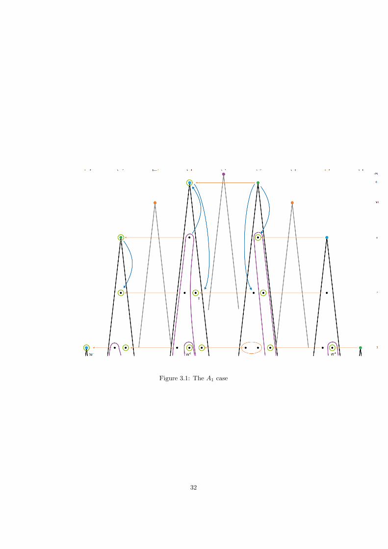
Figure 3.1: The A1 case
32
The orange arrows, going from the Green to the Blue modules and vice versa,represent the short screening operator and the elements in its kernel are encircledwith green colour.We notice that all the elements in the Blue or Green modules on the left borderof this constellation belong to the kernel. Moreover, if an element is in thekernel then it also belongs to the image.The blue arrows represent some examples of the Virasoro action. In particularit is shown the following result:
Proposition 3.8. Defined T = 12
∑i ∂φαi∂φαi∗ +
∑iQi∂
2φαi Energy-Stresstensor as in Theorem 2.19, we have:
L−21 = T
Proof.
L−21 = Y (T )01 = Y (1
2
∑i
∂φαi∂φαi∗ +∑i
Qi∂2φαi)01
=1
2
∑i
Y (∂φαi∂φαi∗) +∑i
QiY (∂2φαi)01)
=1
2
∑i
∑k≥0
〈1, 1〉−k1
k!∂k.∂φαi∂φαi∗ +
∑k≥0
2〈∂φαi , 1〉−k1
k!∂k+1φαi∗ +
∑k≥0
〈∂φαi∂φαi∗, 1〉−k1
k!∂k1
+
+∑i
Qi
∑k≥0
〈1, 1〉−k1
k!∂k.∂2φαi
=
1
2
∑i
∂φαi∂φαi∗ +∑i
Qi∂2φαi = T
in the first and last term of the third line we have k = 0 whereas the secondand third terms vanish.
3.1.4 LCFT WWe now look at the subspace W. In this case, the A1 case, it is known to beequal to the W2-triplet algebra. The elements W−,W0,W+ showed in picture3.1 and studied in [FFHST02], form the adjoint 3-dimensional representation ofg∨ = sl2 acting by long screenings.Since the rank is equal to 1, we have only one short screening operator Z−α/
√2
and so the definition becomes:
W = VΛ⊕ ∩ kerZ−α/√
2
= V√2αZ ∩ kerZ−α/√
2
= V[0] ∩ kerZ−α/√
2.
Since W is a subalgebra of VΛ⊕ , we can now restrict the modules of VΛ⊕ toW-modules and describe their (non-semisimple) decomposition behaviour intoirreducibles.As shown in Corollary 2.35, the Weyl reflections (Z−α/
√2)h
are Virasoro homo-morphisms. Moreover they commute with the W-action by OPE associativity
33
(equation 2.1). Thus they are vertex module homomorphisms for the restric-tion to W and so their kernel and image are W-submodules. In the followingtable we see which values of the power h are associated to the four modulesV[k] := V[ kα
2√
2]:
hV[0] 1V[1] 0V[2] 1V[3] 2
• For the Steinberg module V[1] the commuting map is just the identity sothe kernel is trivial and the image is all. We get then that the modulestays irreducible over W-action and we call it Λ(2).
• For the Facet module V[3], since (Z− α√2)2
= 0, the image is trivial and the
kernel is all. Then again the module stays irreducible and we call it Π(2).
• For the Blue and Green modules, respectively V[0] and V[2], we have instead
that (Z− α√2)1
decomposes them into non-trivial kernel and image. We will
call them Λ(1) and Π(1) and explicitly we have:
Λ(1)→V[0] → Π(1)
Π(1)→V[2] → Λ(1)
To summarize we have the following decompositions:
Λ(1)→V[0] → Π(1)
Π(1)→V[2] → Λ(1)
V[1]∼= Λ(2)
V[3]∼= Π(2)
Remark 3.9. The letters were chosen by Semikhatov to suggest that Λ(1)and Λ(2) have a 1-dimensional groundstates space and Π(1) and Π(2) a 2-dimensional groundstates space.
Remark 3.10. We remark that what we said neither proves that Λ(i),Π(i) areirreducible representations nor that these are all the irreducible representationsof W. However for this particular case, A1, it is proven e.g. in [AM08].
34
Chapter 4
Case Bn, ` = 4
In the previous chapters we introduced a setting, we defined through free-fieldrealization a subspaceW, conjecturally a logarithmic CFT, and then we appliedthe theory to the example of a Lie algebra g with root system A1.In this chapter we will follow again this outline applying it to a new example:the Bn case, ` = 4. This is particularly interesting because it is degenerate ina sense that will be explained later on. To understand the general instance wewill start with the B2 case.
4.1 n = 2
4.1.1 Lattices
Let g be a Lie algebra with root system B2, i.e. g = so(5). Let ` as before bean even integer ` = 2p.Consider as basis of the root lattice ΛR the set {α1, α2} with Killing form:
(α1, α1) = 4 (α2, α2) = 2 (α1, α2) = −2
that means α1 is the long root and α2 the short root.The coroots are then α1
∨ = α1/2, and α2∨ = α2 and so the sets of positive
roots and positive coroots are
Φ+(B2) = {α1, α2, α1 + α2, α1 + 2α2}Φ+(B2
∨) = {α1∨, α2
∨, α1∨ + α2
∨, 2α1∨ + α2
∨}
Therefore
ρg = 3/2 α1 + 2α2
ρg∨ = 2α1
∨ + 3/2 α2∨ = α1 + 3/2 α2
As in the example A1 we now compute the three lattices Λ, Λ⊕, (Λ⊕)∗; thenwe focus on the lattice VOA VΛ⊕ and on its simple modules.
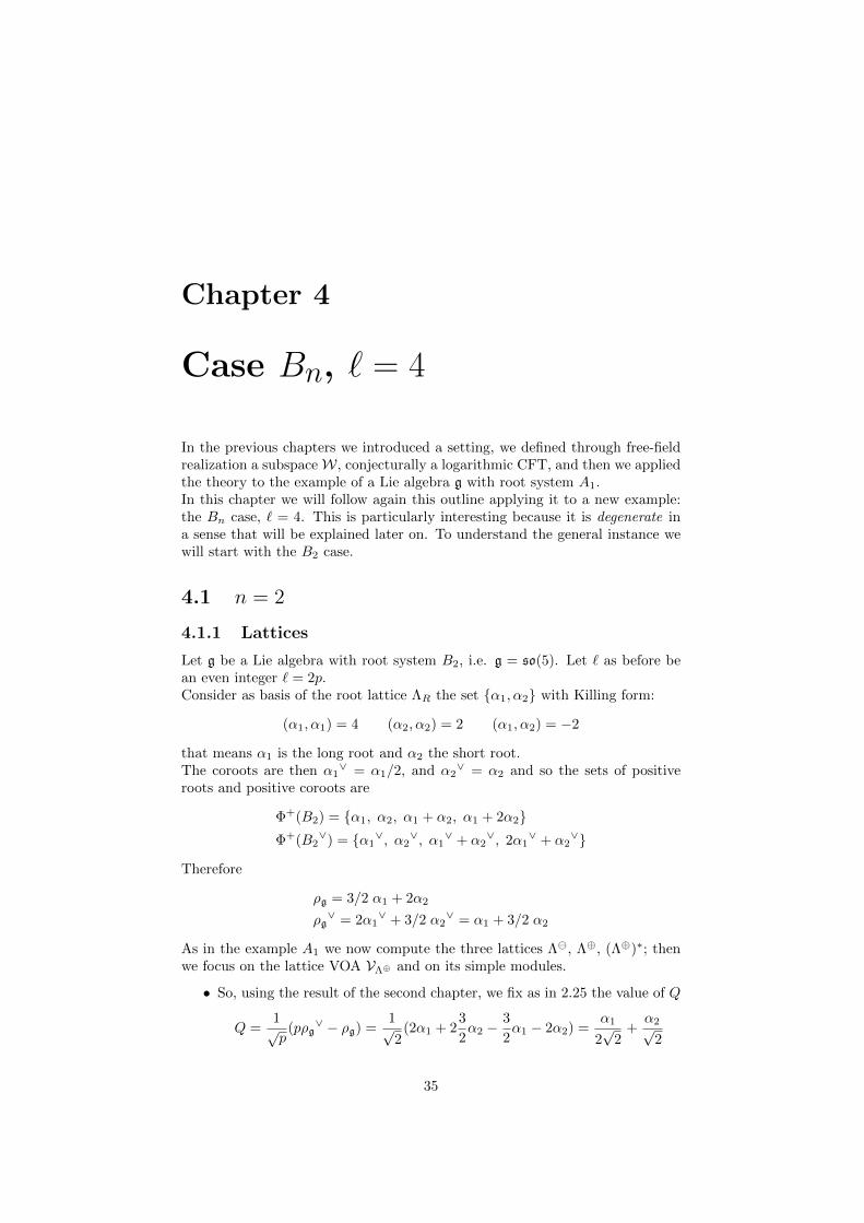
• So, using the result of the second chapter, we fix as in 2.25 the value of Q
Q =1√p
(pρg∨ − ρg) =
1√2
(2α1 + 23
2α2 −
3
2α1 − 2α2) =
α1
2√
2+α2√
2
35
Remark 4.1. In this case, since the dimension is still small, it is possibleto compute Q explicitly (see Appendix).
• The short screening lattice with its basis is in this special case an oddintegral lattice
Λ =1√p
ΛR, {− 1√pα1,−
1√pα2}
• The long screening lattice with its basis is the even integral lattice
Λ⊕ =√pΛR
∨, {√pα1∨,√pα2∨}
Remark 4.2. We recall that if ΛR is the root lattice in the case B2, thenΛR∨ is the root lattice of type C2.
• As last lattice we consider as before the dual of the long screening lattice(Λ⊕)∗ with its basis found by computing the fundamental weights (seeAppendix)
(Λ⊕)∗ =1√p
ΛW {λ1⊕, λ2
⊕} = { α1√p
+α2√p,α1
2√p
+α2√p}
Remark 4.3. λ2⊕ = Q and will be the groundstates representative of one
of the modules V[λ2⊕].
• Now we can compute the number of representations of V⊕Λ :
∣∣(Λ⊕)∗/Λ⊕∣∣ =
∣∣(Λ⊕)∗/Λ∣∣ ∣∣Λ/Λ⊕∣∣ =
∣∣∣∣ 1√p
ΛW /1√p
ΛR
∣∣∣∣ ∣∣∣∣ 1√p
ΛR/√pΛR
∨∣∣∣∣
= |ΛW /ΛR|∣∣∣∣ 1√p
ΛR/√pΛR
∨∣∣∣∣ = 2
∣∣∣∣∣⊕αi
(− 1√pαiZ/
√p(αi)
∨Z)∣∣∣∣∣ =
= 2
∣∣∣∣∣⊕αi
(1√pαiZ/
√p
2
(αi, αi)αiZ
)∣∣∣∣∣ = 2
∣∣∣∣∣⊕αi
Z 2p(αi,αi)
∣∣∣∣∣where |ΛW /ΛR| is obtained by looking explicitly to the cosets or comput-ing the determinant of the Cartan matrix. In our p = 2 case, remem-bering the scalar products (αi, αi), we get that the number of modules is2(p2 · p) = 2 · (1 · 2) = 4.
Specializing to p = 2 above and summarising, our lattices are:
Λ = span{− α1√2,− α2√
2}
Λ⊕ = span{ α1√2,√
2α2}
(Λ⊕)∗ = span{ α1√2
+α2√
2,α1
2√
2+α2√
2}
36
The modules can now be explicitly determined by looking at the cosets in thequotient (Λ⊕)∗/Λ⊕:
[0] [λ2⊕] [λ1
⊕] [λ1⊕ + λ2
⊕]
To make the further description simpler, we give again the previous pictorialnames, i.e. Blue V[0], Steinberg V[λ2
⊕], Green V[λ1⊕] and Facet V[λ1
⊕+λ2⊕] mod-
ule respectively.
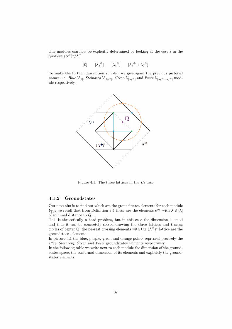
Figure 4.1: The three lattices in the B2 case
4.1.2 Groundstates
Our next aim is to find out which are the groundstates elements for each moduleV[λ]; we recall that from Definition 3.4 these are the elements eφλ with λ ∈ [λ]of minimal distance to Q.This is theoretically a hard problem, but in this case the dimension is smalland thus it can be concretely solved drawing the three lattices and tracingcircles of center Q: the nearest crossing elements with the (Λ⊕)∗ lattice are thegroundstates elements.In picture 4.1 the blue, purple, green and orange points represent precisely theBlue, Steinberg, Green and Facet groundstates elements respectively.In the following table we write next to each module the dimension of the ground-states space, the conformal dimension of its elements and explicitly the ground-states elements:
37
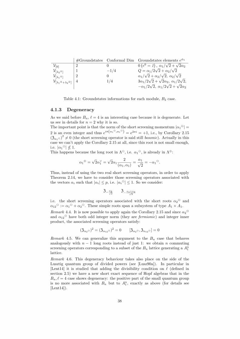
#Groundstates Conformal Dim Groundstates elements eφλ
V[0] 2 0 0(e0 = 1
), α1/
√2 +√
2α2
V[λ2⊕] 1 −1/4 Q = α1/2
√2 + α2/
√2
V[λ1⊕] 2 0 α1/
√2 + α2/
√2, α2/
√2
V[λ1⊕+λ2
⊕] 4 1/4 3α1/2√
2 +√
2α2, α1/2√
2,
−α1/2√
2, α1/2√
2 +√
2α2
Table 4.1: Groundstates informations for each module, B2 case.
4.1.3 Degeneracy
As we said before Bn, ` = 4 is an interesting case because it is degenerate. Letus see in details for n = 2 why it is so.The important point is that the norm of the short screening momentum |α1
| =2 is an even integer and thus eiπ(α1
,α1) = e2πi = +1, i.e., by Corollary 2.15
(Zα1)
2 6= 0 (the short screening operator is said still bosonic). Actually in thiscase we can’t apply the Corollary 2.15 at all, since this root is not small enough,i.e. |α1
| � 1.This happens because the long root in Λ, i.e. α1
, is already in Λ⊕:
α1⊕ =
√2α∨1 =
√2α1
2
(α1, α1)=α1√
2= −α1
.
Thus, instead of using the two real short screening operators, in order to applyTheorem 2.14, we have to consider those screening operators associated withthe vectors αi such that |αi| ≤ p, i.e. |αi| ≤ 1. So we consider:
Z− α2√2
Z−α1+α2√2
i.e. the short screening operators associated with the short roots α2 and
α12 := α1
+ α2. These simple roots span a subsystem of type A1 ×A1.
Remark 4.4. It is now possible to apply again the Corollary 2.15 and since α2
and α12 have both odd integer norm (they are fermionic) and integer inner
product, the associated screening operators satisfy:
(Zα2)2 = (Zα12
)2 = 0 [Zα2 ,Zα12
] = 0
Remark 4.5. We can generalize this argument to the Bn case that behavesanalogously with n − 1 long roots instead of just 1: we obtain n commutingscreening operators corresponding to a subset of the Bn lattice generating a An1lattice.
Remark 4.6. This degeneracy behaviour takes also place on the side of theLusztig quantum group of divided powers (see [Lusz90a]). In particular in[Lent14] it is studied that adding the divisibility condition on ` (defined insection 2.5) we have a new short exact sequence of Hopf algebras that in theBn, ` = 4 case shows degeneracy: the positive part of the small quantum groupis no more associated with Bn but to An1 , exactly as above (for details see[Lent14]).
38
4.1.4 Decomposition behaviour of B2
At this point it is interesting to briefly focus our attention on the decompositionbehaviour of B2 into A1 ×A1 classes.
The relations between the lattices of B2 and A1 ×A1 are the following:
ΛB2 ⊃ Λ(A1×A1)
Λ⊕B2⊃ Λ⊕(A1×A1)
(Λ⊕)∗B2⊂ (Λ⊕)
∗(A1×A1)
On the level of the lattice VOAs we have that VΛ⊕(B2) has got 4 modules,VΛ⊕(A1 ×A1) has got 16 instead.In particular, every VΛ⊕(B2)-module can be restricted to VΛ⊕(A1×A1)-moduleand so decomposes in direct sum of irreducible VΛ⊕(A1×A1)-modules. Explic-itly the cosets decompose:
[Blue] = [0]Bn =
([0]⊕ [α2 +
α12√2
]
)A1×A1
[Steinberg] = [λ2⊕]Bn =
([λ2⊕]⊕ [λ2
⊕ +α2 + α12√
2]
)A1×A1
[Green] = [λ1⊕]Bn
([α2√
2]⊕ [
α12√2
]
)A1×A1
[Facet] = [λ1⊕ + λ2
⊕]Bn =
([λ2⊕ +
α2√2
]⊕ [λ2⊕ +
α12√2
]
)A1×A1
4.1.5 Short screening operators
Let us now go back to the B2 case and look at how the short screening operatorsact in the Blue V[0] and Green V[λ1
⊕] module on the groundstates elements (i.e.conformal dimension equal to 0) and on the higher conformal dimension levelelements (i.e. conformal dimension equal to 1). We will list the results and thenlook at which elements are in the kernel of one or both of the screenings. Tosimplify the notation we will denote
Z1 := Z− α2√2
and Z2 := Z−α1+α2√2
.
Among the elements of conformal dimension 1 we will call inside elements theone below the groundstates elements and outside those which are on top of moreexternal module elements.
1. The screening operators applied to the groundstates elements of the Bluemodule give as results:
• Z1(1) = 0
• Z2(1) = 0
• Z1(eφ α1√
2+√
2α2 ) = eφ (α1+α2)√
2
• Z2(eφ α1√
2+√
2α2 ) = eφ α2√
2
39
2. The screening operators applied to the inside elements of the upper con-formal dimension level of the Blue give as results:
• Z1(∂φ−α2/√
2) = eφ− α2√
2
• Z2(∂φ−α2/√
2) = 0
• Z1(∂φ−(α1+α2)/√
2) = 0
• Z2(∂φ−(α1+α2)/√
2) = eφ− (α1+α2)√
2
• Z1(∂φ(α1+α2)/√
2eφ√
2α1+α2√
2 ) = ∂φ(α1+α2)/√
2eφ (α1+α2)√
2
• Z2(∂φ(α1+α2)/√
2eφ√
2α1+α2√
2 ) = 0
• Z1(∂φ−α2/√
2eφ√
2α1+α2√
2 ) = 0
• Z2(∂φ−α2/√
2eφ√
2α1+α2√
2 ) = ∂φα2/√
2eφ α2√
2
3. The screening operators applied to the outside elements of the upper con-formal dimension level of the Blue give as results:
• Z1(eφ− α1√
2 ) = eφ− (α1+α2)√
2
• Z2(eφ− α1√
2 ) = 0
• Z1(eφ α1√
2 ) = 0
• Z2(eφ α1√
2 ) = eφ− α2√
2
• Z1(eφ√
2(α1+α2)) = 0
• Z2(eφ√
2(α1+α2)) = eφ (α1+α2)√
2
• Z1(eφ√
2α2 )) = eφ α2√
2
• Z2(eφ√
2α2 )) = 0
4. The screening operators applied to the groundstates elements of the Greenmodule give as results:
• Z1(eφ (α1+α2)√
2 ) = 0
• Z2(eφ (α1+α2)√
2 ) = 1
• Z1(eφ α2√
2 ) = 1
• Z2(eφ α2√
2 ) = 0
5. The screening operators applied to the inside elements of the upper con-formal dimension level of the Green give as results:
• Z1((∂φα1/√
2 + ∂φα2/√
2)eφ (α1+α2)√
2 ) = 0
• Z2((∂φα1/√
2 + ∂φα2/√
2)eφ (α1+α2)√
2 ) = 0
40
• Z1(∂φα2/√
2eφ α2√
2 ) = 0
• Z2(∂φα2/√
2eφ α2√
2 ) = 0
• Z1(∂φα2/√
2eφ (α1+α2)√
2 ) = eφ α1√
2
• Z2(∂φα2/√
2eφ (α1+α2)√
2 ) = ∂φα1/√
2
• Z1(∂φ−(α1+α2)/√
2eφ α2√
2 ) = ∂φ−(α1+α2)/√
2
• Z2(∂φ−(α1+α2)/√
2eφ α2√
2 ) = eφ− α1√
2
6. The screening operators applied to the outside elements of the upper con-formal dimension level of the Green give as results:
• Z1(eφ− (α1+α2)√
2 ) = 0
• Z2(eφ (α1+α2)√
2 ) = 0
• Z1(eφ− α2√
2 ) = 0
• Z2(eφ− α2√
2 ) = 0
• Z1(eφ√
2α1+ 3√2α2 ) = eφ
√2(α1+α2)
• Z2(eφ√
2α1+ 3√2α2 ) = e
φ α1√2
+√
2α2
• Z1(eφ α1√
2+ 3√
2α2 )) = e
φ α1√2
+√
2α2
• Z2(eφ α1√
2+ 3√
2α2 )) = eφ
√2α2
In the following picture are shown the kernels of the two short screenings inthe Blue (left) and Green (right) modules. The blue arrows represent Z1, theorange ones Z2.
Remark 4.7. Since (Zi)2 = 0, i = 1, 2 then applying Zi we always land in KerZi.
41
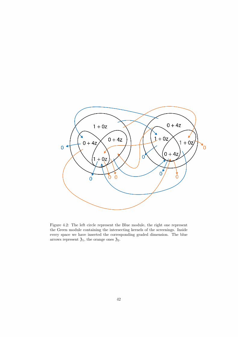
Figure 4.2: The left circle represent the Blue module, the right one representthe Green module containing the intersecting kernels of the screenings. Insideevery space we have inserted the corresponding graded dimension. The bluearrows represent Z1, the orange ones Z2.
42
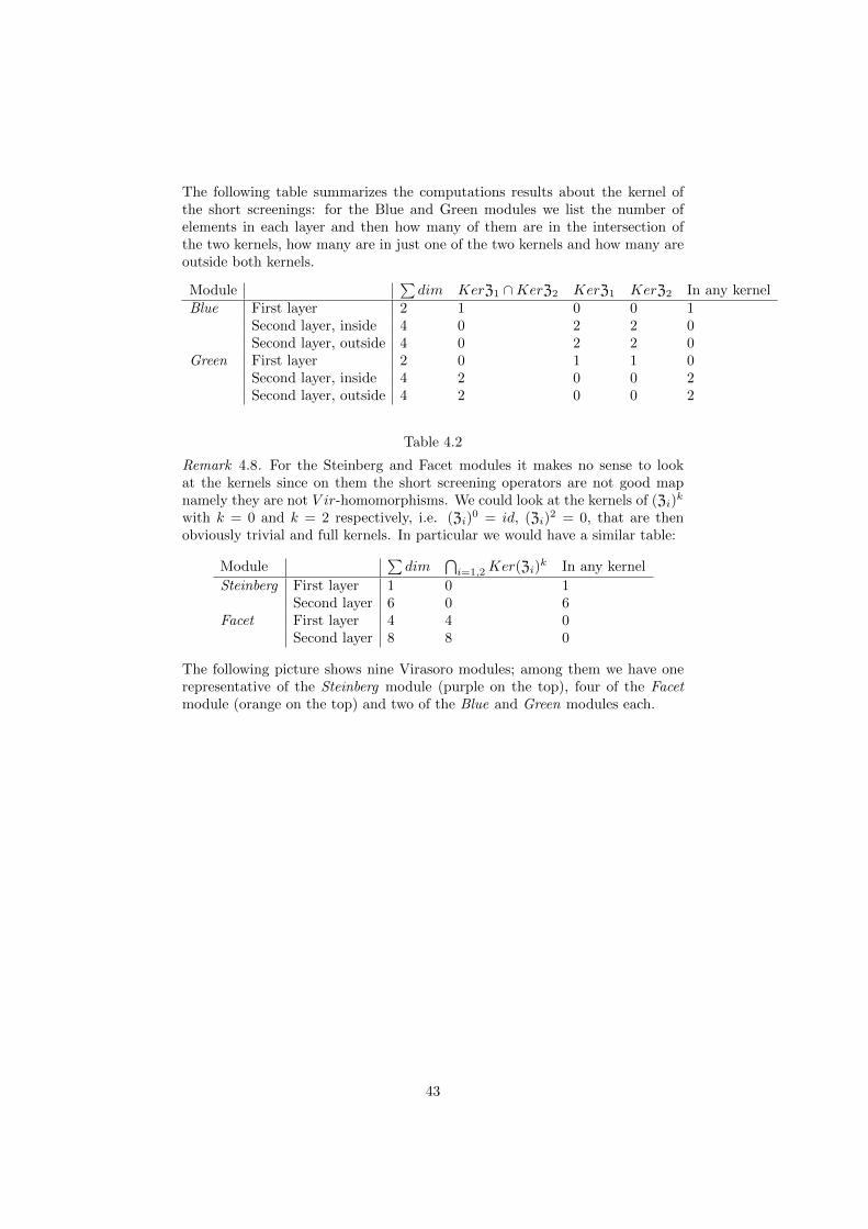
The following table summarizes the computations results about the kernel ofthe short screenings: for the Blue and Green modules we list the number ofelements in each layer and then how many of them are in the intersection ofthe two kernels, how many are in just one of the two kernels and how many areoutside both kernels.
Module∑dim KerZ1 ∩KerZ2 KerZ1 KerZ2 In any kernel
Blue First layer 2 1 0 0 1Second layer, inside 4 0 2 2 0Second layer, outside 4 0 2 2 0
Green First layer 2 0 1 1 0Second layer, inside 4 2 0 0 2Second layer, outside 4 2 0 0 2
Table 4.2
Remark 4.8. For the Steinberg and Facet modules it makes no sense to lookat the kernels since on them the short screening operators are not good mapnamely they are not V ir-homomorphisms. We could look at the kernels of (Zi)
k
with k = 0 and k = 2 respectively, i.e. (Zi)0 = id, (Zi)
2 = 0, that are thenobviously trivial and full kernels. In particular we would have a similar table:
Module∑dim
⋂i=1,2Ker(Zi)
k In any kernel
Steinberg First layer 1 0 1Second layer 6 0 6
Facet First layer 4 4 0Second layer 8 8 0
The following picture shows nine Virasoro modules; among them we have onerepresentative of the Steinberg module (purple on the top), four of the Facetmodule (orange on the top) and two of the Blue and Green modules each.
43
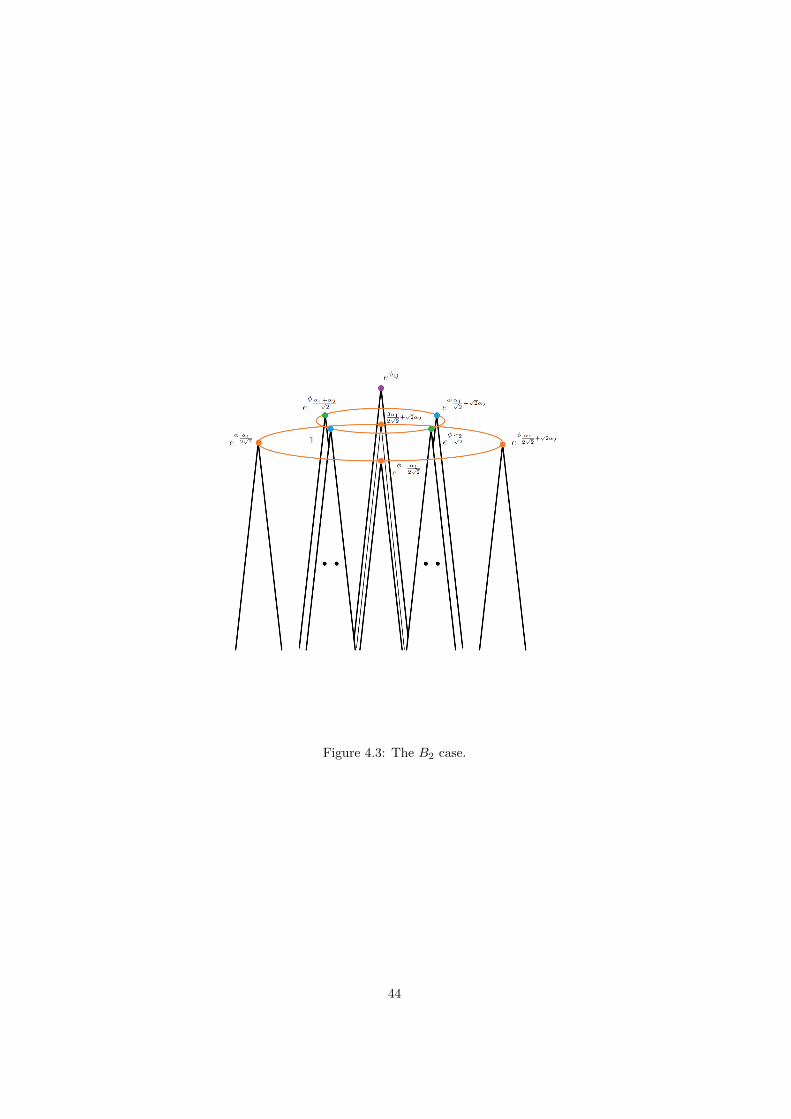
Figure 4.3: The B2 case.
44
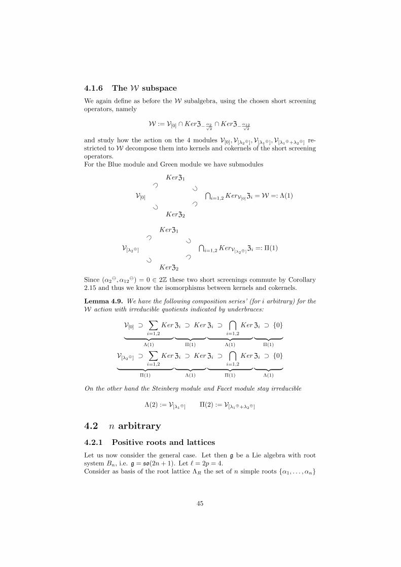
4.1.6 The W subspace
We again define as before the W subalgebra, using the chosen short screeningoperators, namely
W := V[0] ∩KerZ− α2√2∩KerZ−α12√
2
and study how the action on the 4 modules V[0],V[λ2⊕],V[λ1
⊕],V[λ1⊕+λ2
⊕] re-stricted to W decompose them into kernels and cokernels of the short screeningoperators.For the Blue module and Green module we have submodules
KerZ1
⊃ ⊃V[0]
⋂i=1,2KerV[0]
Zi =W =: Λ(1)
⊃ ⊃KerZ2
KerZ1
⊃ ⊃V[λ2
⊕]
⋂i=1,2KerV[λ2
⊕]Zi =: Π(1)
⊃ ⊃KerZ2
Since (α2, α12
) = 0 ∈ 2Z these two short screenings commute by Corollary2.15 and thus we know the isomorphisms between kernels and cokernels.
Lemma 4.9. We have the following composition series’ (for i arbitrary) for theW action with irreducible quotients indicated by underbraces:
V[0] ⊃∑i=1,2
Ker︸ ︷︷ ︸Λ(1)
Zi ⊃ Ker︸ ︷︷ ︸Π(1)
Zi ⊃⋂i=1,2
Ker︸ ︷︷ ︸Λ(1)
Zi ⊃ {0}︸ ︷︷ ︸Π(1)
V[λ2⊕] ⊃
∑i=1,2
Ker︸ ︷︷ ︸Π(1)
Zi ⊃ Ker︸ ︷︷ ︸Λ(1)
Zi ⊃⋂i=1,2
Ker︸ ︷︷ ︸Π(1)
Zi ⊃ {0}︸ ︷︷ ︸Λ(1)
On the other hand the Steinberg module and Facet module stay irreducible
Λ(2) := V[λ1⊕] Π(2) := V[λ1
⊕+λ2⊕]
4.2 n arbitrary
4.2.1 Positive roots and lattices
Let us now consider the general case. Let then g be a Lie algebra with rootsystem Bn, i.e. g = so(2n+ 1). Let ` = 2p = 4.Consider as basis of the root lattice ΛR the set of n simple roots {α1, . . . , αn}
45
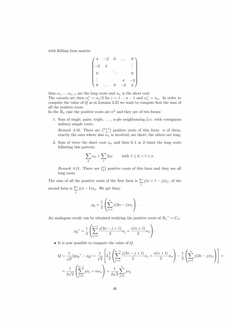
with Killing form matrix:
4 −2 0 . . . 0
−2 4...
0. . . 0
... 4 −20 . . . 0 −2 2
thus α1, . . . αn−1 are the long roots and αn is the short root.The coroots are then α∨i = αi/2 for i = 1 . . . n − 1 and α∨n = αn. In order tocompute the value of Q as in Lemma 2.25 we want to compute first the sum ofall the positive roots.In the Bn case the positive roots are n2 and they are of two forms:
1. Sum of single, pairs, triple, . . . , n-ple neighbouring (i.e. with contiguousindices) simple roots.
Remark 4.10. There are(n+1
2
)positive roots of this form: n of them,
exactly the ones where also αn is involved, are short; the others are long.
2. Sum of twice the short root αn and then 0, 1 or 2 times the long rootsfollowing this pattern:∑
k
αk +∑l
2αl with 1 ≤ k < l ≤ n
Remark 4.11. There are(n2
)positive roots of this form and they are all
long roots.
The sum of all the positive roots of the first form is∑j
j(n + 1 − j)αj , of the
second form is∑j
j(n− 1)αj . We get then:
ρg =1
2
n∑j=1
j(2n− j)αj
.
An analogous result can be obtained studying the positive roots of Bn∨ = Cn:
ρg∨ =
1
2
n−1∑j=1
j(2n− j + 1)
2αj +
n(n+ 1)
2αn
.
• It is now possible to compute the value of Q
Q =1√p
(pρg∨ − ρg) =
1√2
21
2
n−1∑j=1
j(2n− j + 1)
2αj +
n(n+ 1)
2αn
− 1
2
n∑j=1
j(2n− j)αj
=
=1
2√
2
n−1∑j=1
jαj + nαn
=1
2√
2
n∑j=1
jαj
46
• The short screening lattice with its basis is in this special case an oddintegral lattice
Λ =1√2
ΛR, {− 1√2α1, . . . ,−
1√2αn}
• The long screening lattice with its basis is an even integral lattice
Λ⊕ =√
2ΛR∨,
{√2α1∨, . . . ,
√2αn
∨}
=
{α1√
2, . . . ,
αn−1√2,√
2αn
}• And finally the dual of the long screening lattice with its basis, found
through the known fundamental weights, is
(Λ⊕)∗ =1√2
ΛW {λ1⊕, . . . , λn
⊕} = { α1√2
+ . . .+αn√
2,α1√
2+
2√2
(α2 + . . .+ αn) , . . .
. . . ,α1√
2+
2√2α2 + . . .+
i− 1√2αi−1 +
i√2
(αi + . . .+ αn) ,1
2√
2(α1 + 2α2 + . . .+ nαn)}
Remark 4.12. As in the B2 case 4.1 we obtain the equality λn⊕ = Q.
• Let us compute the number of representations of V⊕Λ :
∣∣(Λ⊕)∗/Λ⊕∣∣ =
∣∣(Λ⊕)∗/Λ∣∣ ∣∣Λ/Λ⊕∣∣ = 2
∣∣∣∣∣⊕αi
Z 2p(αi,αi)
∣∣∣∣∣= 2
∣∣Zp × Zp/2 × Zp/2 × · · · × Zp/2∣∣ =
= 2 |Z2 × Z× Z× · · · × Z| = 4
where again we obtained |(Λ⊕)∗/Λ| = 2 by looking at the determinantof the Cartan matrix
|〈αi, αj〉| = 2
∣∣∣∣ (αi, αj)(αj , αj)
∣∣∣∣ =
∣∣∣∣∣∣∣∣∣∣
2 −1
−1. . .
. . .
. . .. . . −1−1 2
∣∣∣∣∣∣∣∣∣∣
= 2
or explicitly looking at the cosets with respect to Λ:
(Λ⊕)∗/Λ ={
0 + Λ, Q+ Λ}
• Thus, since Λ/Λ⊕ ={
0 + Λ⊕, αn√2
+ Λ⊕}
, our 4 modules are given by
the cosets[0], [
αn√2
], [Q], [Q+αn√
2]
respectively the Blue, Green, Steinberg and Facet module.
47
4.2.2 Groundstates
Now, as in the A1 and B2 case we would like to determine the groundstates ele-ments. In the lower dimensional case this was a drawing or easy-computationalproblem; in the n dimension case we can proceed in two ways: the more heuristicone, that generalizes those results, and the sharper one, that follows the wrongwalks approach.
Theorem 4.13. The groundstates elements of each module in the Bn case arethe ones listed in the following table together with the dimension of the associatedgroundstates space:
Blue Q+ 12
n∑k=1
εkαk...n, such that
∏i εi = 1 2n−1
Steinberg Q 1
Green Q+ 12
n∑k=1
εkαk...n , such that
∏i εi = −1 2n−1
Facet Q± αk...n 2n
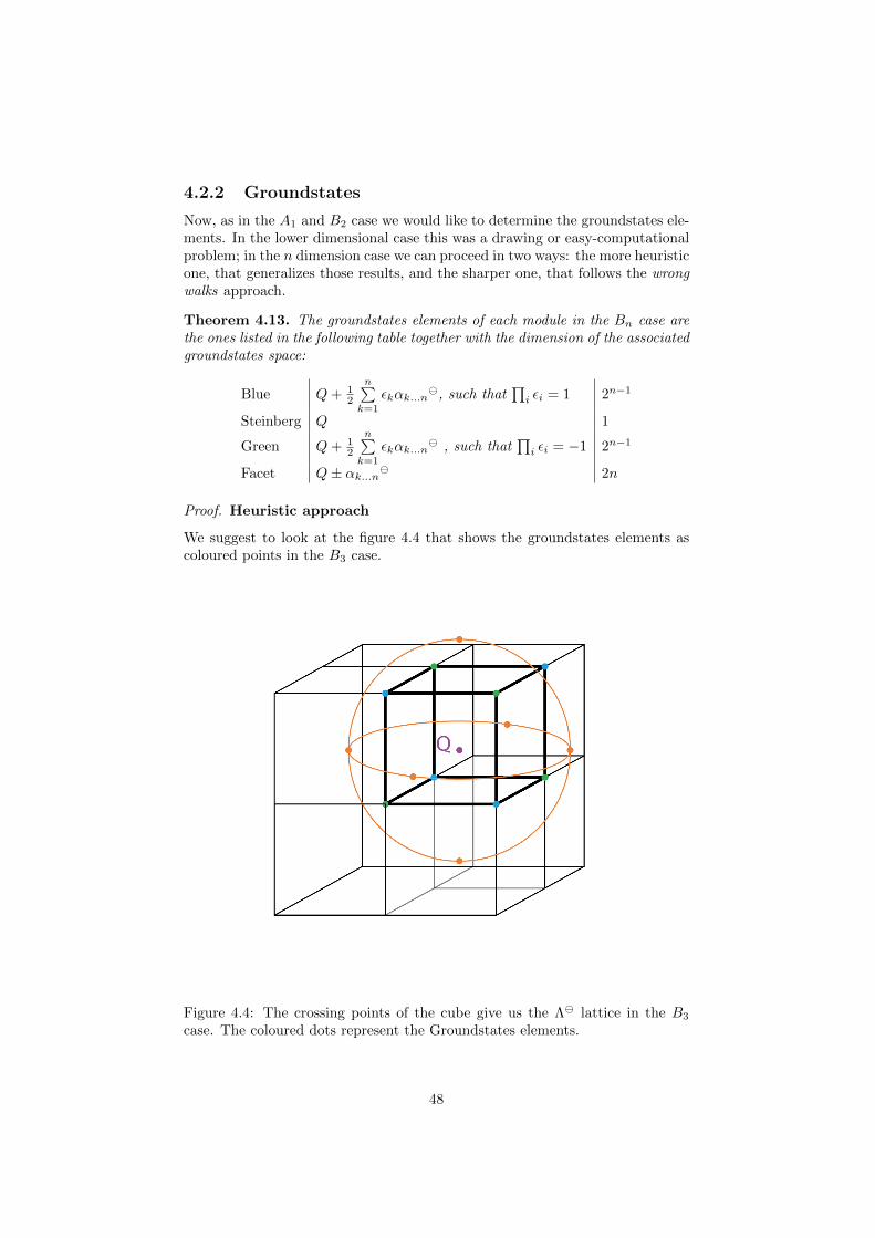
Proof. Heuristic approach
We suggest to look at the figure 4.4 that shows the groundstates elements ascoloured points in the B3 case.
Figure 4.4: The crossing points of the cube give us the Λ lattice in the B3
case. The coloured dots represent the Groundstates elements.
48
We can think at the groundstates elements constellation as located on a n-dimensional hypercube and on a (n − 1)-dimensional sphere (for n = 1 a lineand a pair of points, for n = 2 a square and a circle, for n = 3 a 3-dimensionalcube and a 2-dimensional sphere in the 3-dimensional space). The hypercubeedge and the sphere radius are equal to the short screenings length; the centerof both is in the Steinberg point Q.With this picture in mind we can now place the Blue and Green representativegroundstates elements alternating on the vertices of the hypercube. The Facetrepresentative groundstates elements are instead on those sphere points suchthat tracing a line from them to Q, we cross the hyperplane in the center of the(n− 1)-faces.So we obtain that the Steinberg module (purple in the figure) has always justone dimensional groundstates space. The dimension of the groundstates spaceof the Blue and Green modules together is equal to the number of vertices i.e.2n, so they have a 2n−1 dimensional groundstates space each. The dimensionof the groundstates space of the Facet module (orange in the figure) is insteadequal to the number of (n− 1)-faces i.e. 2n.
Sharper approach
We now try to define these groundstates elements in a clearer, less heuristic way.We consider, as in the case n = 2, the very short roots of Λ i.e.
αk...n := αk
+ . . .+ αn, k = 1, . . . , n
with αnn := αn
. We notice that if we sum αk...n to a vector of the lattice
it just moves one component of it, namely the k-th component.We then consider the set of vectors Γ =
{12αk...n
with k ∈ {1, . . . , n}}
. They
are a basis of (Λ⊕)∗A1
n and since they are all orthogonal and of the same length,they form a Zn-lattice.What we will do is moving from the starting pointQ to the surroundings throughthese vectors. In this way we will cross the nearest points to Q of (Λ⊕)
∗Bn
: thosewill be the wanted groundstates elements.
• Q is obviously the only groundstates element of the Steinberg module.
• Summing just one vector of Γ we don’t land in (Λ⊕)∗Bn
, so the vectors of
the form Q± 12αk...n
are not groundstates elements.
• Analogously summing several vectors of Γ but not all of them, we againdon’t reach any (Λ⊕)
∗Bn
element.
• To get a (Λ⊕)∗Bn
element we have to sum all of them, i.e.{Q+ 1
2
n∑k=1
εkαk...n}
with εk ∈ {±1}. In this case:
– we reach an elements of the Blue module ←→∏k
εk = 1
– we reach an elements of the Green module ←→∏k
εk = −1
This result give us again the dimension of the groundstates space: the
number of combinations
{Q+ 1
2
n∑k=1
εkαk...n}
with εk ∈ {±1} are 2n.
49
The ones corresponding to the Blue case, i.e.∏k
εk = 1 and to the case
Green case i.e.∏k
εk = −1 are half of them namely 2n−1.
• Finally if we sum the double of a vector of Γ we get Q± αk...n and thisis in (Λ⊕)
∗Bn
, in particular it is in the Facet module. So these are all theFacet groundstates element.The dimension of the groundstates space of the Facet module results againequal to 2n since we can reach them summing or subtracting n vectors⇒ (n+ n) = 2n.
4.3 Conformal dimension of the grounstates
We now want to compute the conformal dimension.
Lemma 4.14. The conformal dimension of the Steinberg, Blue, Green andFacet modules are −n8 , 0, 0 and 4−n
8 respectively.
Proof. • To calculate the conformal dimension of the Steinberg module it isthen sufficient to compute:
1
2(Q,Q)− (Q,Q) = −1
2(Q,Q)
where the value of Q is the one found in 4.2, namely Q = 12√
2
n∑j=1
jαj .
(Q,Q) = (1
2√
2
n∑j=1
jαj ,1
2√
2
n∑j=1
jαj)
=1
8(
n∑j=1
jαj ,
n∑j=1
jαj)
=1
8
n∑j=1
j2(αj , αj) + 2
n−1∑j=1
(jαj , (j + 1)αj+1)
=
1
8
n−1∑j=1
j2 · 4 + n2 · 2 + 2
n−1∑j=1
j(j + 1)(−2)
=
1
8
−4
n−1∑j=1
j + 2n2
=
1
8
[−4
(n− 1)n
2+ 2n2
]=
1
8· 2n
Then the conformal dimension of the Steinberg module is equal to −n8• For the Blue and Green module the calculation is similar. We choose as
representative the groundstates element Q + 12
n∑k=1
αk...n, i.e., the one
50
with εk = 1 ∀k. The computation becomes:
1
2(Q+
1
2
n∑k=1
αk...n, Q+
1
2
n∑k=1
αk...n)− (Q+
1
2
n∑k=1
αk...n, Q)
= −1
2(Q,Q) +
1
2(1
2
n∑k=1
αk...n,
1
2
n∑k=1
αk...n)
= −n8
+1
8(
n∑k=1
αk...n,
n∑k=1
αk...n)
= −n8
+1
8(
n∑j=1
jαj,
n∑j=1
jαj)
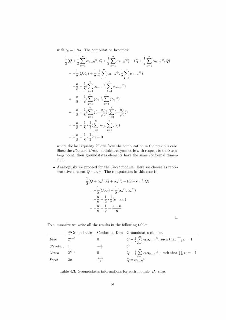
= −n8
+1
8(
n∑j=1
j(− αj√2
),
n∑j=1
(− αj√2
))
= −n8
+1
8· 1
2(
n∑j=1
jαj ,
n∑j=1
jαj)
= −n8
+1
8· 1
22n = 0
where the last equality follows from the computation in the previous case.Since the Blue and Green module are symmetric with respect to the Stein-berg point, their groundstates elements have the same conformal dimen-sion.
• Analogously we proceed for the Facet module. Here we choose as repre-sentative element Q+ αn
. The computation in this case is:
1
2(Q+ αn
, Q+ αn)− (Q+ αn
, Q)
= −1
2(Q,Q) +
1
2(αn, αn
)
= −n8
+1
2· 1
2(αn, αn)
= −n8
+1
2=
4− n8
To summarize we write all the results in the following table:
#Groundstates Conformal Dim Groundstates elements
Blue 2n−1 0 Q+ 12
n∑k=1
εkαk...n, such that
∏i εi = 1
Steinberg 1 −n8 Q
Green 2n−1 0 Q+ 12
n∑k=1
εkαk...n , such that
∏i εi = −1
Facet 2n 4−n8 Q± αk...n
Table 4.3: Groundstates informations for each module, Bn case.
51
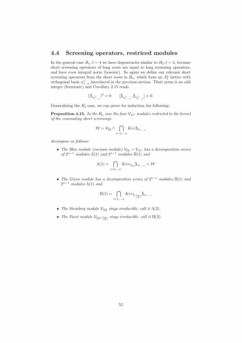
4.4 Screening operators, restriced modules
In the general case Bn, ` = 4 we have degeneracies similar to B2, ` = 4, becauseshort screening operators of long roots are equal to long screening operators,and have even integral norm (bosonic). So again we define our relevant shortscreening operators from the short roots in Bn, which form an An1 lattice withorthogonal basis αi...n introduced in the previous section. Their norm is an oddinteger (fermionic) and Corollary 2.15 reads
(Zαi...n)2 = 0 [Zαi...n
,Zαj...n] = 0.
Generalizing the B2 case, we can prove for induction the following:
Proposition 4.15. In the Bn case the four VΛ⊕ modules restricted to the kernelof the commuting short screenings
W = V[0] ∩⋂
i=1,...n
KerZαi...n
decompose as follows:
• The Blue module (vacuum module) V[0] = VΛ⊕ has a decomposition seriesof 2n−1 modules Λ(1) and 2n−1 modules Π(1) and
Λ(1) =⋂
i=1,...n
KerV[0]Zαi...n =W
• The Green module has a decomposition series of 2n−1 modules Π(1) and2n−1 modules Λ(1) and
Π(1) =⋂
i=1,...n
KerV[αn√
2]Zαi...n
• The Steinberg module V[Q] stays irreducible, call it Λ(2).
• The Facet module V[Q+αn√2
] stays irreducible, call it Π(2).
52
Chapter 5
Comparison with theSymplectic Fermions
In Chapter 4 we constructed the VOA W in the case g = Bn, ` = 4. We willcall it WBn,`=4.While studying this structure we conjectured that it has the same representationcategory of a known VOA, the Symplectic Fermions VOA.We will now introduce the Symplectic Fermions VOA and present some resultsthat convinced us of the plausibility of this conjecture.We want anyway to highlight that we later proved the conjecture in a strongerform, showing that these VOAs are even isomorphic. The proof is displayed inChapter 6.
5.1 The Symplectic Fermions VOA
The vertex algebra of a single pair of symplectic fermions VSF = VSF1is a
super-vertex algebra (VOSA) with central charge −2 introduced by [Kausch00].Our exposition follows [DR16]: in vertex algebra language, the symplecticfermions are generated by two fermionic fields ψ,ψ∗, explicitly
ψ(z) =∑n∈Z
ψ−n−1zn ψ∗(z) =
∑n∈Z
ψ∗−n−1zn
fulfilling the following anticommutators
[ψn, ψ∗m]+ = nδn+m=0 id
Remark 5.1. This super-vertex algebra can equivalently be described with thefollowing construction: we can first consider a purely odd super-vector space hover C of dimension 2, h = 〈x, y〉 ∼= C0|2: from it we can construct a structure,
called the affine Lie super-algebra h of free super-bosons. This has a module, thevacuum h-module, that carries the structure of a vertex operator super-algebraVSF , the symplectic fermion VOSA.
Similarly one defines the super-vertex algebra of n-pairs of symplectic fermions
VSFn = (VSF1)n
53
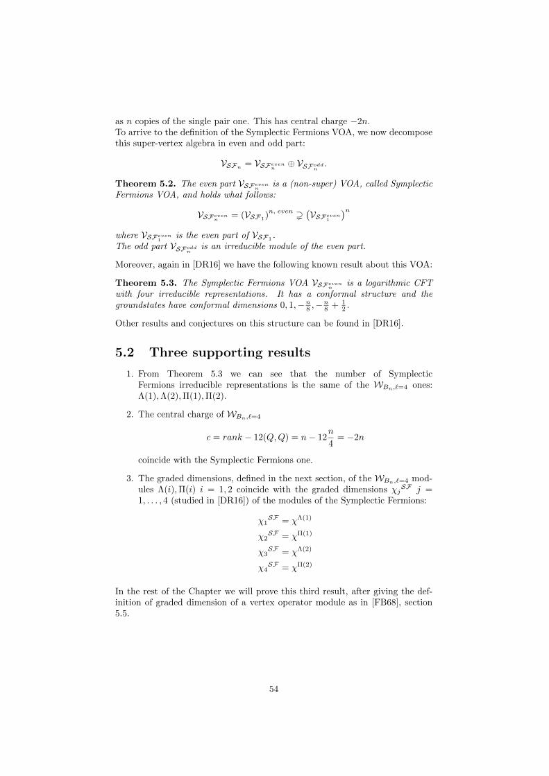
as n copies of the single pair one. This has central charge −2n.To arrive to the definition of the Symplectic Fermions VOA, we now decomposethis super-vertex algebra in even and odd part:
VSFn = VSFevenn⊕ VSFoddn
.
Theorem 5.2. The even part VSFevennis a (non-super) VOA, called Symplectic
Fermions VOA, and holds what follows:
VSFevenn= (VSF1
)n, even )
(VSFeven1
)nwhere VSFeven1
is the even part of VSF1 .The odd part VSFoddn
is an irreducible module of the even part.
Moreover, again in [DR16] we have the following known result about this VOA:
Theorem 5.3. The Symplectic Fermions VOA VSFevennis a logarithmic CFT
with four irreducible representations. It has a conformal structure and thegroundstates have conformal dimensions 0, 1,−n8 ,−
n8 + 1
2 .
Other results and conjectures on this structure can be found in [DR16].
5.2 Three supporting results
1. From Theorem 5.3 we can see that the number of SymplecticFermions irreducible representations is the same of the WBn,`=4 ones:Λ(1),Λ(2),Π(1),Π(2).
2. The central charge of WBn,`=4
c = rank − 12(Q,Q) = n− 12n
4= −2n
coincide with the Symplectic Fermions one.
3. The graded dimensions, defined in the next section, of the WBn,`=4 mod-ules Λ(i),Π(i) i = 1, 2 coincide with the graded dimensions χj
SF j =1, . . . , 4 (studied in [DR16]) of the modules of the Symplectic Fermions:
χ1SF = χΛ(1)
χ2SF = χΠ(1)
χ3SF = χΛ(2)
χ4SF = χΠ(2)
In the rest of the Chapter we will prove this third result, after giving the def-inition of graded dimension of a vertex operator module as in [FB68], section5.5.
54
5.3 Graded dimension
Definition 5.4. Let V be a conformal vertex algebra of central charge c. LetM =
⊕nMn be a graded module of V, with Mn finite dimensional ∀n. We define
the graded dimension, or character, of M , as the formal power series
dimM = q−c24
∑n
dimMnqn.
We compute now the graded dimension of each Virasoro module and from thatthe one of the VΛ⊕-modules.
Proposition 5.5. The graded dimension of a Virasoro module Vλ is
dimVλ =q
12 (Q−λ,Q−λ)
η(q)n
Proof. The Virasoro modules Vλ ={ueφλ with u differential polynomial
}are
graded by the conformal dimension. We will call E0 := 12 (λ, λ)− (λ,Q) so that
the degrees are of the form E0 + k with k ∈ N0.For rank = 1 the graded dimension of a general Virasoro module Vλ with topelement eφλ will then be:
dimVλ = q−c24
(qE0 + qE0+1 + 2qE0+2 + 3qE0+3 + 5qE0+4 + . . .
)(5.1)
= q−c24
∑k∈N0
pkqE0+k (5.2)
where pk denotes the number of possible combinations u of differential elementswith |u| equal to k.In our case c is the Virasoro central charge c = rank−12(Q,Q) = 1−12(Q,Q),so Formula 5.1 becomes:
dimVλ = q[− 124 (1−12(Q,Q))+ 1
2 (λ,λ)−(λ,Q)]∑k∈N0
pkqk
= q12 (Q−λ,Q−λ)q−
124
∑k∈N0
pkqk
Now∑k∈N0
pkqk is again the dimension of a graded space i.e. the space
N :=⊗k∈N0
C[∂kφ]
We compute it:∑k∈N0
pkqk = dimN =
∏k∈N
dimC[∂kφ] =∏k∈N
∑h∈N0
qhk =∏k∈N
1
1− qk
55
Now we recognise that q−124
∏k∈N
11−qk is the inverse of the Dedekind eta function
η(q) (defined for istance in [Kob93]).Thus the dimension of the Virasoro module Mλ is equal to:
dimVλ =q
12 (Q−λ,Q−λ)
η(q)
Similarly in arbitrary rank = n:
dimVλ =q
12 (Q−λ,Q−λ)
η(q)n
Proposition 5.6. The graded dimension of a VΛ⊕ modules V[µ] is:
dim(V[µ]) = χ[µ] =Θ[Q−µ]
η(q)n=
∑λ∈[µ]
q12 (Q−λ,Q−λ)
[q124
∏k∈N
(1− qk)]n
Proof. To compute the graded dimension of a module V[µ] of VΛ⊕ , since for 2.3V[µ] =
⊕λ∈[µ] Vλ, we have now to sum among the graded dimensions of the
Virasoro modules Vλ with λ ∈ [µ] coset of (Λ⊕)∗/Λ⊕.We consider the general case rank = n arbitrary and the Jacobi theta function(defined for istance in [HW59])
Θ[Q−µ](q) :=∑λ∈[µ]
q12 (Q−λ,Q−λ)
to get finally the graded dimension
dim(V[µ]) = χ[µ] =Θ[Q−µ]
η(q)n=
∑λ∈[µ]
q12 (Q−λ,Q−λ)
[q124
∏k∈N
(1− qk)]n
5.4 Symplectic Fermions characters
We now copy from [DR16] first the functions:
χns,+ = (q124
∞∏m=1
(1 + qm))2n χns,− = (q124
∞∏m=1
(1− qm))2n
χr,+ = (q−148
∞∏m=1
(1 + qm−12 ))2n χr,− = (q−
148
∞∏m=1
(1− qm− 12 ))2n
used to define the characters of the modules of the Symplectic Fermions:
χ1SF =
1
2(χns,+ + χns,−) χ2
SF =1
2(χns,+ − χns,−)
χ3SF =
1
2(χr,+ + χr,−) χ4
SF =1
2(χr,+ − χr,−)
56
5.5 Comparison
The claim is that the graded dimensions computation support the conjecture ofthe category equivalence between W(Bn)-Rep and SFn −Rep by showing
χ3SF = χΛ(2) = χV[1]
χ4SF = χΠ(2) = χV[3]
2n−1(χ1SF + χ2
SF ) = 2n−1(χΛ(1) + χΠ(1)) = χV[0] = χV[2]
In particular, χ1SF and χ2
SF should give us the graded dimension of the kernelof the screening in the Blue and Green modules respectively. The factor 2n−1
counts all the possible combinations of kernel of short screenings.
We will now prove this claim building the proof from the A1 case and arrivingto the arbitrary n case. But first, we show it in the n = 2 case as a consequenceof the results of section 4.1.5.
5.5.1 First approximate comparison for n = 2
Going briefly back to section 4.1.5, we can notice that, for n = 2, table 4.2tells us the first terms of the graded dimensions of Λ(1) and Π(1) since thesemodules are given by the intersection of the kernels in the Blue and Greenmodule respectively. In this case c = −2n = −4; they are
χΛ(1) ≈ q− c24 (1 + 0q) ≈ q 1
6 (1 + 0q)
χΠ(1) ≈ q− c24 (0 + 4q) ≈ q 1
6 (0 + 4q)
We now make a first approximate comparison, computing the characters χ1SF
and χ2SF of the modules of the symplectic fermions VOA for n = 2 up to the
second power. We ignore the multiplied term q124 .
χns,+ ≈ q16 (1 + q)4(1 + q2)4 . . . ≈q 1
6 (1 + 4q + 6q2 + . . .)(1 + 4q2 + . . .) . . . ≈ q 16 (1 + 4q + 10q2 + . . .)
χns,− ≈ q16 (1− q)4(1− q2)4 . . . ≈q 1
6 (1− 4q + 6q2 + . . .)(1− 4q2 + . . .) . . . ≈ q 16 (1− 4q + 2q2 + . . .)
⇒ χ1SF =
1
2(χns,+ + χns,−) ≈ 1
2q
16 (2 + 12q2) ≈ q 1
6 (1 + 0q + 6q2)
⇒ χ2SF =
1
2(χns,+ − χns,−) ≈ 1
2q
16 (8q + 8q2) ≈ q 1
6 (0 + 4q + 4q2)
so the results match.
5.5.2 Proofs for n = 1
The next results are true for the A1 case, i.e. for n = 1.
Lemma 5.7.χns,+ = χ1
SF + χ2SF = χV[0] = χV[2]
Proof. Let us compute the graded dimension of the Blue module V[0] and com-pare it to χns,+. We said that for [µ] ∈ (Λ⊕)∗/Λ⊕, the graded dimension is:
χ[µ] =Θ[Q−µ](q)
η(q)=
∑λ∈[µ]
q12 (Q−λ,Q−λ)
q124
∞∏m=1
(1− qm)
57
In the case of [µ] equal to the Blue module V[0] namely in the case of elements
of the form kα2√
2with k ≡ 0 (4), we have:
1
2(Q− λ,Q− λ)− 1
2(Q,Q) =
1
2(kα
2√
2,kα
2√
2)− (
α
2√
2,kα
2√
2) =
1
8(k2 − 2k)
⇒ 1
2(Q− λ,Q− λ) =
1
8(k2 − 2k + 1)
and so the dimension turns out to be:
χV[0] = q18 q−
124
∑k≡0(4)
q18 (k2−2k)
∞∏m=1
(1− qm)= q
224
∑rq2(r2− r2 )
∞∏m=1
(1− qm)
where r := k/4.Now, to compare it to χns,+ we use the Jacobi triple product ([HW59]), namely:
∞∑m=1
w2mqm2
=
∞∏m=1
(1− q2m)(1 + w2q2m−1)(1 + w−2q2m−1)
Substituting q = q2 and w = q12 we can rewrite the sum above as follows:
χV[0] =q224
∞∏m=1
(1− q4m)(1 + q−1q4m−2)(1 + qq4m−2)
∞∏m=1
(1− qm)
=q224
∞∏m=1
(1− q4m)(1 + q4m−3)(1 + q4m−1)
∞∏m=1
(1− qm)
=q224
∞∏m=1
(1− qm)(1 + qm)(1 + q2m)(1 + q4m−3)(1 + q4m−1)
∞∏m=1
(1− qm)
=q224
∞∏m=1
(1 + qm)(1 + q2m)(1 + q4m−3)(1 + q4m−1)
This result is exactly the expected
χns,+ = q224
∞∏m=1
(1 + qm)2
since (1 + q2m) give us all the even terms and (1 + q4m−3)(1 + q4m−1) the oddones of (1 + qm).
58
For the Green module V[2] the computation is the same. The Green elements
are of the form kα2√
2with k ≡ 2 (4) that brings us to:
χV[2] = q224
∑rq2(r2+ r
2 )
∞∏m=1
(1− qm)
So the only thing that is changing is in the nominator the plus in the power ofq that implies just a switch between the last to terms of the final product:
∞∏m=1
(1 + qm)(1 + q2m)(1 + q4m−1)(1 + q4m−3)
The result holds the same. So we have, as claimed:
χV[0] = χV[2] = χns,+
In the same way we can say something about the Steinberg V[1] and the FacetV[3] modules. In this case χ3
SF and χ4SF should give us directly their graded
dimensions.
Lemma 5.8.χ3SF = χV[1] χ4
SF = χV[3]
Proof. Here the computation is slightly harder. The reason is that in this casewe have to deal with χ3
SF and χ4SF that are sums of two products. Thus, it
is not convenient to proceed as before. We follow an other strategy.The trick consist in looking at the two modules together: we can namely considerthe sum of their graded dimensions and then split them using the fact that forthe Steinberg module we have integral powers such as qm and for the Facetmodule fractional ones q
12 +m.∑
k≡1(4)
q18 (k2−2k+1) =
1
2(∑k≡1(2)
q18 (k−1)2
+∑k≡1(2)
q18 (k−1)2
)
where we define q such that: q12 = −q 1
2 . In this way we have that if k ≡ 3(4)we catch a minus sign and the terms vanish. If instead k ≡ 1(4) the terms getsummed and multiplying them by 1
2 we get the equality. Now we can indicatek = 2r + 1
1
2
∑k≡1(2)
(q12 )
14 (k−1)2
+∑k≡1(2)
(−q 12 )
14 (k−1)2
=1
2
(∑r
(q12 )r
2
+∑r
(−q 12 )r
2
)
Proceeding as before, we use the Jacobi triple product to write the graded di-
59
mension as sum of products:
1
2q−
124
∞∏m=1
(1− qm)(1 + qm−12 )(1 + qm−
12 )
∞∏m=1
(1− qm)+
∞∏m=1
(1− qm)(1− qm− 12 )(1− qm− 1
2 )
∞∏m=1
(1− qm)
=
1
2q−
124
( ∞∏m=1
(1 + qm−12 )(1 + qm−
12 ) +
∞∏m=1
(1− qm− 12 )(1− qm− 1
2 )
)
=1
2(χr,+ + χr,−) = χ3
SF
The Facet case is complementary: if k ≡ 3 (4) the terms have to be summedand if k ≡ 1 (4), the terms have to be erased. In order to get that we put aminus in the expression above:∑
k≡3(4)
q18 (k2−2k+1) =
1
2(∑k≡1(2)
q18 (k−1)2
−∑k≡1(2)
q18 (k−1)2
)
that proceeding as before turns out to be exactly:
1
2(χr,+ − χr,−) = χ4
SF
So, as we claimed we reached the following:
χ3SF = χV[1] χ4
SF = χV[3]
5.5.3 Proofs for arbitrary n
We now generalize these proofs to the n dimensional case. We start with apreparatory result that for simplicity we prove for n = 2, but holds for arbitraryn:
Lemma 5.9. Consider [λ] ∈ (Λ⊕A12)∗/Λ⊕A1
2 , which in the A12 coordinates
with basis {α1⊕, α12
⊕ = α1⊕ + α2
⊕} has the form: λ = λ1α1⊕ + λ2α12
⊕.Then we have the following relation between the associated Jacobi theta func-tions:
Θ[λ] = Θ[λ1] ·Θ[λ2]
Proof. We write λ = x + k where x ∈ (Λ⊕A12)∗ and k ∈ Λ⊕A1
2 and we writealso x and k in coordinates:
x = x1α1⊕ + x2α12
⊕ k = k1α1⊕ + k2α12
⊕
where k1, k2 ∈ Z and x1, x2 can be also fractional.Then, decomposing also Q = Q1α1
⊕ +Q2α12⊕ with Q1, Q2 fractional, we get:
‖λ−Q‖2 = ‖x1α1⊕ + x2α12
⊕ + k1α1⊕ + k2α12
⊕ −Q1α1⊕ −Q2α12
⊕‖2
= ‖(x1 + k1 −Q1)α1⊕ + (x2 + k2 −Q2)α12
⊕‖2
= ‖(x1 + k1 −Q1)α1⊕‖2 + ‖(x2 + k2 −Q2)α12
⊕‖2
60
So the Theta function, using the associativity of the product, becomes:
Θ[λ−Q] =∑
λ=x+k
q12 (λ−Q,λ−Q) =
∑k1,k2
q12‖(x1+k1−Q1)α1
⊕‖2+ 12‖(x2+k2−Q2)α12
⊕‖2
=
(∑k1
q12‖(x1+k1−Q1)α1
⊕‖2)·
(∑k2
q12‖(x2+k2−Q2)α12
⊕‖2)
=
( ∑λ1=x1+k1
q12 (λ1−Q1,λ1−Q1)
)( ∑λ2=x2+k2
q12 (λ2−Q2,λ2−Q2)
)= Θ[λ1−Q] ·Θ[λ2−Q]
We will use now this result to compute the graded dimension of the modules forarbitrary n. We start from the Blue V[0] and Green V[αn√
2] modules.
Lemma 5.10.
χV[0] = χV[αn√
2]
= 2n−1(χ1SF + χ2
SF ) = 2n−1χns,+
Proof. To prove this result we will use
1. the fact that these two modules have the same structure and thus theyhave the same graded dimension
2. the fact that the sum of them gives the ΛA1n lattice
3. Lemma 5.9.
ΘV[0]=
∑λ∈0+Λ⊕Bn
q12 (Q−λ,Q−λ)
=(1)
1
2
∑λ∈0+Λ⊕Bn
q12 (Q−λ,Q−λ) +
∑λ∈αn+Λ⊕Bn
q12 (Q−λ,Q−λ)
=(2)
1
2
∑λ∈ΛA1
n
q12 (Q−λ,Q−λ)
=(3)
1
2
∑λ∈ΛA1
q12 (Q−λ,Q−λ)
n
Now we proceed as in the case n = 1:
λ ∈ ΛA1⇐⇒ λ = −mα√
2, m ∈ N
Then the graded dimension can be written:
χV[0] =
12
( ∑λ∈ΛA1
q12 (Q−λ,Q−λ)
)nηn
=1
2
∞∑m=1
q12 (m2+m+ 1
4 )
q124
∞∏m=1
(1− qm)
n
61
Finally we use again the Jacobi triple product to conclude:
=1
2
(q
18 · q− 1
24
∞∏m=1
(1− qm)(1 + q12 qm−
12 )(1 + q−
12 qm−
12 )
(1− qm)
)n
=1
2
(q
224
∞∏m=1
(1 + qm)(1 + qm−1)
)n
=1
2q
2n24
((1 + q1−1)
∞∏m=1
(1 + qm)2
)n
=1
2q
2n24 2n
( ∞∏m=1
(1 + qm)
)2n
= 2n−1χns,+
We now want this matching result also for the Steinberg V[Q] and FacetV[Q+αn/
√2] modules. We could proceed as for n = 1, but it is interesting
to follow another path which uses the decomposition behaviour of Bn intoA1 × . . . × A1 coordinates. To make it understandable we first present theresult in the B2 case.
Notation 5.11. χi will denote the character associated with the ith dimensioni.e. to Ai1.χj will denote the characters of Symplectic Fermions (instead of χj
SF ).
Lemma 5.12. In the B2 case we have:
χV[Q] = χ32
Proof. We consider the class of (Λ⊕B2)∗/Λ⊕B2
and we want to write it as sumof classes of (Λ⊕A1
2)∗/Λ⊕A12 as in 4.1.4. We have again:
[Q]B2=
([Q]⊕ [Q+
α2 + α12√2
]
)A1
2
= ([Q]⊕ [−Q])A12
Hence in the character we can decompose the sum:
χV[Q] =
∑λ∈Q+Λ⊕B2
q12 (Q−λ,Q−λ)
η2
=
∑λ∈Q+Λ⊕A1
2
q12 (Q−λ,Q−λ) +
∑λ∈−Q+Λ⊕A1
2
q12 (Q−λ,Q−λ)
η2
=Θ2
[Q]
η2+
Θ2[−Q]
η2
Now the class [−Q] in A12 can be written in A1 × A1 coordinates as (Facet
module × Facet module) and thus the second term is the square of the gradeddimension of the Facet module for n = 1. The first term is instead simply the
62
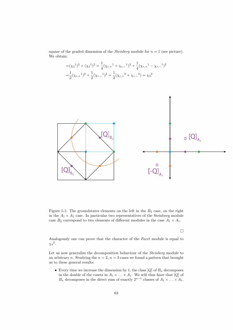
square of the graded dimension of the Steinberg module for n = 1 (see picture).We obtain:
=(χ31)2 + (χ4
1)2 =1
4(χr,+
1 + χr,−1)2 +
1
4(χr,+
1 − χr,−1)2
=1
2(χr,+
1)2 +1
2(χr,−
1)2 =1
2(χr,+
2 + χr,−2) = χ3
2
Figure 5.1: The groundstates elements on the left in the B2 case, on the rightin the A1 × A1 case. In particular two representatives of the Steinberg modulecase B2 correspond to two elements of different modules in the case A1 ×A1.
Analogously one can prove that the character of the Facet module is equal toχ4
2.
Let us now generalize the decomposition behaviour of the Steinberg module toan arbitrary n. Studying the n = 2, n = 3 cases we found a pattern that broughtus to these general results:
• Every time we increase the dimension by 1, the class [Q] of Bn decomposesin the double of the cosets in A1× . . .×A1. We will thus have that [Q] ofBn decomposes in the direct sum of exactly 2n−1 classes of A1× . . .×A1.
63
• In particular it decomposes in combination of classes of A1 associated tothe Steinberg and the Facet modules.
• The combination follows the Pascal’s triangle; more precisely the coeffi-cient of the combination of the Steinberg and the Facet classes are theeven powers coefficients of the expansion of the n-th power of a binomial.
From these three results we have that the graded dimension of the Steinbergmodule is given by the graded dimensions of the one dimensional Steinberg andFacet modules combined in a binomial form:
χ[Q] =
n/2∑k=0
(n
2k
)(χ3
1)n−2k(χ41)2k
if n even, otherwise the sum arrives to n−12 .
Analogously for the Facet module we obtain the coefficients related to the oddpowers:
χ[Q+αn/√
2] =
(n−2)/2∑k=0
(n
2k + 1
)(χ3
1)n−2k−1(χ41)2k+1
if n even, otherwise the sum arrives to n−12 .
This result, as we can see, matches with our claim:
1
2(χ[Q] + χ[Q+αn/
√2]) =
=1
2
n/2∑k=0
(n
2k
)(χ3
1)n−2k(χ41)2k +
(n−2)/2∑k=0
(n
2k + 1
)(χ3
1)n−2k−1(χ41)2k+1
=
1
2
[n∑k=0
(n
k
)(χ3
1)n−k(χ41)k)
]
=1
2(χ3
1 + χ41)n = (χns,+
1)n
= χns,+n =
1
2(χ3
n + χ4n)
64
Chapter 6
Isomorphism of VOAs
As we mentioned in Chapter 5, at the end of this project we proved a re-sult stronger than the one conjectured: our VOA WBn,`=4 and the SymplecticFermions VOA VSFevenn
are isomorphic.We will now show this proof step by step: we first prove it for A1 = B1 and thenwe generalize it to the n dimensional case using that the super-vertex algebrajust consists of n copies of the one-dimensional one.
Lemma 6.1. For the datum g = A1, ` = 4 the lattice Λ = 1√2ΛR is an odd
integral lattice. We have the following isomorphisms of super-vertex algebrasand vertex algebras
VSF1= KerVΛ
Z−α/√
2
VSFeven1
∼=WA1,`=4
Proof. This seems to be common knowledge (see e.g. [FGST06a]), but let usdraw a quick proof: we define an isomorphisms from VSF1 to VΛ that sendsthe states (defined in 5.1) as follows
ψ 7−→ eφ−α/√
2
ψ∗ 7−→ ∂eφ+α/√
2
This maps lands clearly in KerZ−α/√2since
Z−α/√
2(eφ−α/√
2) = 0 Z−α/√
2(∂eφ+α/√
2) = ∂Z−α/√
2(eφ+α/√
2) = ∂.1 = 0
and the OPE between the images is the same as the one of the sources insymplectic fermions, in our language:
Y (eφ−α/√
2)∂eφ+α/√
2 =∑k≥0
⟨eφ−α/
√2 , ∂φα/
√2
⟩⟨eφ−α/
√2 , eφα/
√2
⟩eφα/
√2zk
∂k
k!eφ−α/
√2
+∑k≥0
⟨eφ−α/
√2 , eφα/
√2
⟩∂φα/
√2eφα/√
2zk∂k
k!eφ−α/
√2
=∑k≥0
z−1zk∂eφ+α/√
2∂k
k!eφ−α/
√2 +
∑k≥0
(+z−2)zkeφ+α/√
2∂k
k!eφ−α/
√2
= e0z−2 + 0 z−1 + · · ·
65
If we want to explicitly prove the defining relations of the mode operators
Y (ψ, z) = ψ(z) =∑n∈Z
Y (ψ)nzn
Y (ψ∗, z) = ψ∗(z) =∑n∈Z
Y (ψ∗)nzn
[Y (ψ)−1−n, Y (ψ∗)−1−m]+ = mδm+n=0
for the images Y (a)−1−n, Y (b)−1−m from the previous calculation of Y (a)b, weinvoke the associativity formula for integer OPE’s (as in [Thiel94], here of asuper-vertex algebra)
[Y (a)−1−n, Y (b)−1−m]+ =∑l≥0
(n
l
)Y (Y (a)−l−1b)l−(1+n+m)
=
(n
0
)Y (0)−(1+n+m) +
(n
1
)Y (e0)1−(1+n+m)
= nδn+m=0 id
arriving to the wanted result.Now, we can think about the VOAs as modules over themselves, i.e. as thetwo vacuum representations, and use the found results. In particular, since thevacuum representation of VSF1 is irreducible, the vertex algebra homomorphismis injective: the Kernel must be a trivial subrepresentation and can not be all,since the image is non-zero.Analogously, surjectivity follows from the matching of the graded dimensionscalculated above: the dimensions of the two vacuum modules match, indeed.So we found a bijective map
VSF1←→ KerVΛ
Z−α/√
2.
It is easy to see that the even subspace VSFeven1, i.e. differential polynomials in
ψ,ψ∗ with an even number of factors in each monomial, maps precisely to thesubspace with Λ-degrees in Λ⊕ = 2Λ hence
VSFeven1
∼= kerVΛ⊕Z−α/
√2 =WA1,`=4
Corollary 6.2. By tensoring n copies we get
VSFn =
(kerV 1√
2ΛR,A1
Z−α/√
2
)n=
⋂i=1,...n
kerV 1√2
ΛR,An1
Z−α
An1i /√
2
Now we want to prove that the result of Corallary 6.2 holds taking the evenpart on both sides. The even part of VSFn is again completely characterized
66
by its lattice-degrees: They are the sublattice Λ ⊂ 1√2ΛR,An1 = Zn consisting of
even sums of the basis elements, i.e.
Λ =
{∑i
xi(αAn1i /√
2) | xi ∈ Z,∑i
xi ∈ 2Z
}⊂ Zn
But this Λ is precisely the Dn-root lattice, which is equal to the rescaled rootlattice 1√
2Cn, which is in turn the rescaled coroot lattice
√2B∨n . And this is
precisely the lattice Λ⊕ for Bn, ` = 4 and the images of the orthogonal basis arethe dual short roots:
Λ =√
2Λ∨R,Bn = Λ⊕Bn,`=4 αAn1i /√
2 = αBni...n/√
2
which we prescribed in 4.2.2 as short screening momenta in the degenerate caseBn, ` = 4. Altogether this gives our final result
Corollary 6.3.
VSFevenn=
⋂i=1,...n
kerV√2Λ∨R,Bn
Z−αBni...n∼=WBn,`=4
67
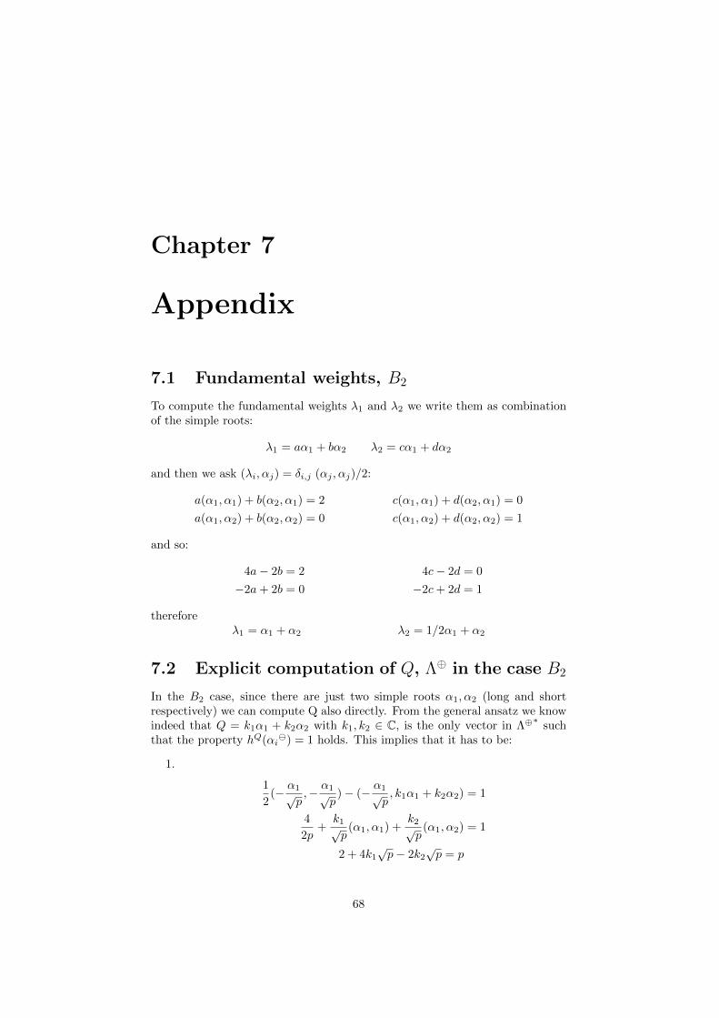
Chapter 7
Appendix
7.1 Fundamental weights, B2
To compute the fundamental weights λ1 and λ2 we write them as combinationof the simple roots:
λ1 = aα1 + bα2 λ2 = cα1 + dα2
and then we ask (λi, αj) = δi,j (αj , αj)/2:
a(α1, α1) + b(α2, α1) = 2 c(α1, α1) + d(α2, α1) = 0
a(α1, α2) + b(α2, α2) = 0 c(α1, α2) + d(α2, α2) = 1
and so:
4a− 2b = 2 4c− 2d = 0
−2a+ 2b = 0 −2c+ 2d = 1
thereforeλ1 = α1 + α2 λ2 = 1/2α1 + α2
7.2 Explicit computation of Q, Λ⊕ in the case B2
In the B2 case, since there are just two simple roots α1, α2 (long and shortrespectively) we can compute Q also directly. From the general ansatz we knowindeed that Q = k1α1 + k2α2 with k1, k2 ∈ C, is the only vector in Λ⊕
∗such
that the property hQ(αi) = 1 holds. This implies that it has to be:
1.
1
2(− α1√
p,− α1√
p)− (− α1√
p, k1α1 + k2α2) = 1
4
2p+
k1√p
(α1, α1) +k2√p
(α1, α2) = 1
2 + 4k1√p− 2k2
√p = p
68
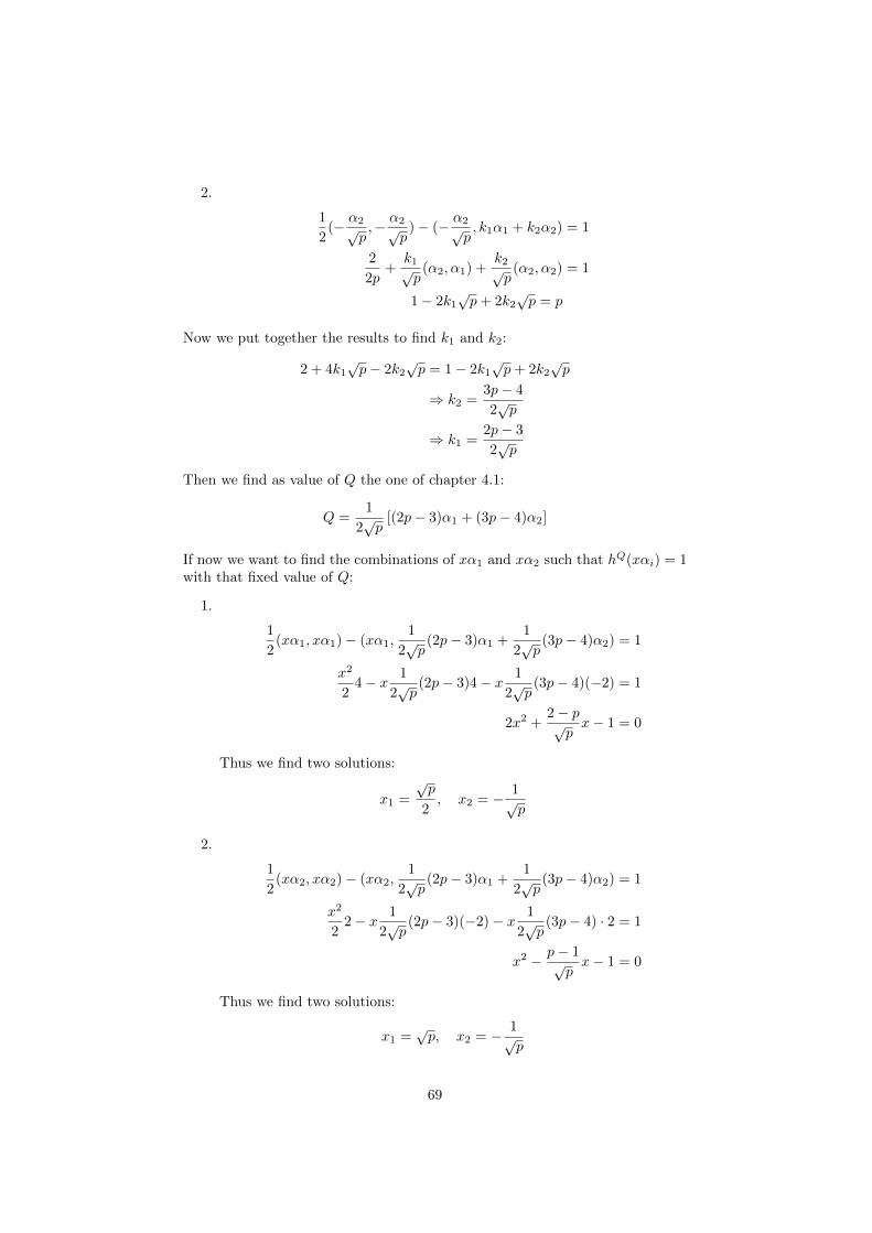
2.
1
2(− α2√
p,− α2√
p)− (− α2√
p, k1α1 + k2α2) = 1
2
2p+
k1√p
(α2, α1) +k2√p
(α2, α2) = 1
1− 2k1√p+ 2k2
√p = p
Now we put together the results to find k1 and k2:
2 + 4k1√p− 2k2
√p = 1− 2k1
√p+ 2k2
√p
⇒ k2 =3p− 4
2√p
⇒ k1 =2p− 3
2√p
Then we find as value of Q the one of chapter 4.1:
Q =1
2√p
[(2p− 3)α1 + (3p− 4)α2]
If now we want to find the combinations of xα1 and xα2 such that hQ(xαi) = 1with that fixed value of Q:
1.
1
2(xα1, xα1)− (xα1,
1
2√p
(2p− 3)α1 +1
2√p
(3p− 4)α2) = 1
x2
24− x 1
2√p
(2p− 3)4− x 1
2√p
(3p− 4)(−2) = 1
2x2 +2− p√px− 1 = 0
Thus we find two solutions:
x1 =
√p
2, x2 = − 1
√p
2.
1
2(xα2, xα2)− (xα2,
1
2√p
(2p− 3)α1 +1
2√p
(3p− 4)α2) = 1
x2
22− x 1
2√p
(2p− 3)(−2)− x 1
2√p
(3p− 4) · 2 = 1
x2 − p− 1√px− 1 = 0
Thus we find two solutions:
x1 =√p, x2 = − 1
√p
69
So we found again our four solutions:
α1⊕ :=
√p
2α1 α1
:= − 1√pα1
α2⊕ :=
√pα2 α2
:= − 1√pα2
70
Bibliography
[AM08] D. Adamovic, A. Milas , On the triplet vertex algebra W(p), Advancesin Mathematics, 217 (2008) 2664-2699
[DR16] A. Davydov, I. Runkel, Holomorphic Symplectic Fermions, (2016)arXiv:1601.06451v1
[EO03] P. Etingof, V. Ostrik Finite tensor categories (2003)arXiv:math/0301027
[FB68] E. Frenkel, D. Ben-Zvi Vertex Algebras and Algebraic Curves AmericanMathematical Society
[FF88] B. L. Feigin, E. V. Frenkel: A family of representations of affine Lie al-gebras, Uspekhi Mat. Nauk, 43:5(263) (1988), 227-228. English Translation:Russian Mathematical Surveys(1988),43(5):221
[FFHST02] J. Fjelstad, J. Fuchs, S. Hwang, A.M. Semikhatov, I.Yu.Tipunin, Logarithmic conformal field theories via logarithmic deformations,Nucl.Phys. B633 (2002) 379-413
[FGST06a] B.L. Feigin, A. M. Gainutdinov, A. M. Semikhatov, I. Yu. Tipunin,Kazhdan-Lusztig correspondence for the representation category of the tripletW-algebra in logarithmic CFT, Theor.Math.Phys. 148 (2006) 1210-1235;Teor.Mat.Fiz. 148 (2006) 398-427.
[HW59] G. H. Hardy, E. M. Wright An Introduction to the Theory of Numbers(1959) Oxford: Clarendon Press
[Kassel95] C. Kassel, Quantum Groups (1995) Graduate Texts in Mathematics,Springer-Verlag New York
[Kausch95] H.G Kausch, Curiosities at c = −2, (1995) arXiv:hep-th/9510149
[Kausch00] H. G. Kausch, Symplectic Fermions (2000) Nucl. Phys. B 583 , p.513-541.
[Kob93] N. Koblitz, Introduction to Elliptic Curves and Modular Forms Grad-uate Texts in Mathematics 97 (1993), Springer-Verlag
[Lent07] S. Lentner Vertex Algebras Constructed from Hopf Algebra Structures(2007) Diploma Thesis
[Lent14] S. Lentner, A Frobenius homomorphism for Lusztig’s quantum groupsfor arbitrary roots of unity., (2014) arXiv:1406.0865
71
[Lent17] S. Lentner, Quantum Groups and Nichols Algebras acting on Confor-mal Quantum Field Theories, (2017) arXiv:1702.06431v1
[Lusz90a] G. Lusztig, Finite-dimensional Hopf algebras arising from quantizeduniversal enveloping algebras, Journal of the AMS Vol. 3/1 (1990), 257-296.
[NT11] K. Nagatomo and A. Tsuchiya, The Triplet Vertex Operator AlgebraW (p) and the Restricted Quantum Group Uq(sl2) at 1 = e
πıp ,
[Runkel12] I. Runkel, A braided monoidal category for free super-bosons, (2012)Preprint, arXiv:1209.5554.
[TF09] B.L. Feigin, I. Yu. Tipunin, Logarithmic CFTs connected with simple liealgebras, (2009) arXiv:1002.5047
[Thiel94] K. Thielemans, An algorithmic approach to Operator Product Expan-sions, W-algebras and W-strings, (1994), arXiv:hep-th/9506159
[TW13] A. Tsuchiya, S. Wood, The tensor structure on the representation cat-egory of the Wp triplet algebra, J. Phys. A: Math. Theor. 46 (2013) 445203.(2011), arXiv:0902.4607
72
Acknowledgement
First of all I would like to thank my supervisors: Giovanna Carnovale for sup-porting me to go to Hamburg and being always patient and helpful, and SimonLentner for the daily motivation and care that made me feel welcome from thevery first moment.Then I would like to thank my family: my parents, Emanuele, Nina, Niccolo,Nora, Claudia, Nicola, Marta and Fabio, for the unlimited love.Finally I would like to thank my second family, my friends spread all over Europethat despite the distance are always with me.
73


![Universit a degli Studi di Padova - Benvenuti su [email protected]](https://img.pdfslide.tips/doc/110x75/623144e01cb07c303d32a836/universit-a-degli-studi-di-padova-benvenuti-su-emailprotected.jpg)