Embed Size (px)
Citation preview
Universita degli Studi di Milano
Facolta di Scienze Matematiche Fisiche e Naturali
Corso di Laurea in Fisica
Anna Miglio
Cooperative Jahn-Teller effect in LiNiO2
Relatore: Nicola Manini
Correlatore: Giovanni Onida
Correlatore: Jeroen van den Brink
Anno Accademico 2004/2005

ii
Contents
1 Introduction 11.1 Cooperative Jahn-Teller effect in crystals . . . . . . . . . . . . . . . . 11.2 Nickel oxides : LiNiO2 and NaNiO2 . . . . . . . . . . . . . . . . . . . 2
2 Numerical techniques 72.1 DFT . . . . . . . . . . . . . . . . . . . . . . . . . . . . . . . . . . . . 72.2 The ABINIT code . . . . . . . . . . . . . . . . . . . . . . . . . . . . . 10
3 Test calculations for NiO 153.1 Structure of NiO . . . . . . . . . . . . . . . . . . . . . . . . . . . . . 163.2 Convergency calculations . . . . . . . . . . . . . . . . . . . . . . . . . 18
3.2.1 Convergence with respect to Ecutoff . . . . . . . . . . . . . . . 18
3.2.2 Convergence: ~k-point mesh and smearing parameter . . . . . . 203.3 The NiO lattice parameter . . . . . . . . . . . . . . . . . . . . . . . 213.4 NiO band structure and magnetic ordering . . . . . . . . . . . . . . . 23
4 LiNiO2 294.1 Structure and system energetics . . . . . . . . . . . . . . . . . . . . . 29
4.1.1 Optimization of the geometry . . . . . . . . . . . . . . . . . . 354.1.2 Jahn-Teller distortions . . . . . . . . . . . . . . . . . . . . . . 35
4.2 Bands . . . . . . . . . . . . . . . . . . . . . . . . . . . . . . . . . . . 39
5 Conclusions and discussion 47
Ringraziamenti 51
iii

iv CONTENTS
Chapter 1
Introduction
The Jahn-Teller effect encompasses several different phenomena, from the distortionsof high-symmetry molecules and molecular ions, to the physics of many isolateddefects in high-symmetry (e.g. cubic) crystals, to the collective distorted phasesof several solids. All these phenomena have in common a spontaneously brokensymmetry to a distorted phase producing a lowering in electronic energy associatedto a splitting of some electronic configuration which is otherwise degenerate in high-symmetry geometry.
Several equivalent (or sometimes inequivalent) distortions are usually realized,each associated to a different electronic state. Thermal or quantum tunneling amongthe local minima restores the broken symmetry to a state (known as dynamical J-Teffect) which is deeply non-adiabatic in nature. This possibility is realized by molec-ular and impurity J-T systems, where the energy barriers separating the differentminima are finite. In contrast, cooperative J-T crystals can only distort statically toone of the several equivalent configurations, where they remain trapped with macro-scopically large barriers to equivalent distortions.
1.1 Cooperative Jahn-Teller effect in crystals
Collective distortions of J-T solids affect the mechanical and electronic properties ofthese materials in several different ways. Characteristically, the J-T distortion is ob-served as a finite-temperature phase transition from a high-temperature undistortedphase (often accompanied by locally fluctuating distortions) to a low-temperaturecollectively distorted phase. The phase transition occurs at a temperature Tc suchthat kBTc is of the order of the characteristic energy gained by the J-T distortion ofa typical chemical unit in the lattice.
The cooperative J-T distortion leads to (typically small, but finite) macroscopicchanges in density and, more importantly, shape of the solid sample. Different ener-
1
2 CHAPTER 1. INTRODUCTION
getically equivalent static distortions lead to geometrically different changes in shapeof the crystal. The boundary geometric constraints of a packing of different micro-crystals take advantage of the different equivalent distortions. Macroscopically largecrystals instead may undergo severe damages near the phase transition due to hugestrains at the boundary between regions where distortions at different equivalentminima could have developed. This type of phenomena is especially important inmaterials such as the manganites (LaMnO3) where the J-T distortion is large.
Also the undistorted high-temperature phase is of significant interest, since thetendency to incoherently fluctuating local distortions can lead to anomalously largeDebye-Waller factors and to anomalous response functions of the conducting elec-trons. In fact the electronic state of a crystal is a band state, and typically the J-Tcollective distortion affects the crystal bands.
The J-T effect might also have an important role in determining the magneticbehavior of many compounds e.g. Transition Metal compounds and rare earth com-pounds; Jahn-Teller can be held responsible not only for their structural propertiesbut also for their magnetic structure. Within this class of materials,we are inter-ested in compounds containing magnetic ions whose ground-state is characterized byhaving an orbital degeneracy as well as spin degeneracy.
1.2 Nickel oxides : LiNiO2 and NaNiO2
Transition metal (TM) oxides show interesting electronic, magnetic and structuralproperties and thus are still a subject of constant attention and research, also inview of possible applications. LiNiO2, NaNiO2 and other TM oxides such as LiCoO2
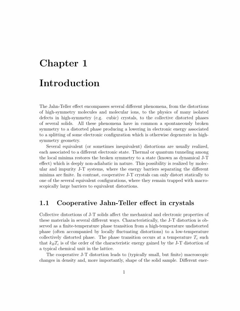
are roughly isostructural; they all crystallize with a rhombohedral rock-salt structure(Fig. 1.1). Metal ions occupy the octahedral sites of an approximately cubic close-packed network of oxygens ions to form ordered layers of Ni and Li ions. In particular,in LiNiO2 the triangular layers are orthogonal to the (111) direction of the cubic rock-salt structure. Unlike the cuprates and manganites that have a corner shared networkof octahedra, LiNiO2 has an edge-shared network of NiO6 octahedra. The corner-shared network of MO6 octahedra has linear M-O-M bonds which can be distortedmore easily than in edge-shared networks as two M are linked by two oxygens ionsthus making the bond more rigid.
In particular, layered oxides that belong to the AMO2 family (A=Li, Na andM=Ni, Fe, Co) are very promising materials for battery applications. Several workshave been devoted to the magnetic properties of LiNiO2 but the results remain con-troversial. Since this material is crucial for battery capacity, solid-state chemistshave improved the synthesis and the characterization of the samples. It has beenshown that both electro-chemical and magnetic properties are very sensitive to thedeparture from stoichiometry often represented symbolically by the chemical for-
1.2. NICKEL OXIDES : LINIO2 AND NANIO2 3
Figure 1.1: The idealized crystal structure of LiNiO2, as depicted in Goodenough[1]. Actually LiNiO2’s structure is not cubic as the distance between successive Ni3+
triangular planes in the (111) direction is slightly shorter than the ideal cubic valueas determined by the in-plane spacings.
4 CHAPTER 1. INTRODUCTION
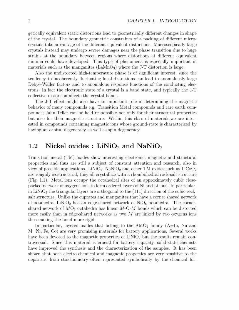
Figure 1.2: The splitting of Ni3+ (S=1/2) 3d orbitals in the octahedral field of thesix neighboring oxygens atoms.
mula Li1−xNi1+xO2, 0.02 ≤ x ≤ 0.20, depending on the experimental conditionsof the synthesis process. While NaNiO2 can be characterized as being an A-typeanti-ferromagnetic insulator with a ferrodistorsive orbital ordering due to the cooper-ative Jahn-Teller effect of the Ni3+ ions in the low spin state, the magnetic structureof LiNiO2 is still partly unclear. The absence of long-range magnetic and orbitalordering in LiNiO2, indeed observed in isostructural NaNiO2, has not been fully un-derstood and explained yet. Rougier et AP . [2, 3] reports the existence of a NiO6
octahedra distortion: two different Ni-O bond lengths with four short bonds of 1.91A and two of 2.09 A. On the basis of this EXAFS analysis, this difference is seenas a local Jahn-Teller effect of the Ni3+ ion. The analysis has been performed overquasi-stoichiometric LiNiO2 and considering quasi-stoichiometric LiNiO2 being in anordered structure made of NiO2 slabs even though diffraction studies would be nec-essary to prove it without ambiguity. The synthesis of quasi-stoichiometric LiNiO2
is necessary to a clear interpretation of EXAFS data as the non-stoichiometric char-acter of this compound would not allow to distinguish whether the existence of twobond lengths is due to the J-T effect of nickel trivalent ions (t62e
1) (in Fig.1.2) in theoctahedral environment (NiO2 slab made of NiO6 edge-sharing octahedra, see figuresin Sec.4 or to the different ionic radii of Ni3+ and Ni2+. As mentioned above, LiNiO2
true formula Li1−xNi1+xO2 indicates the presence of extra nickel ions in substitution
1.2. NICKEL OXIDES : LINIO2 AND NANIO2 5
of lithium ones. As a result, a certain amount of nickel ions (2x) are in the divalentstate (t62e
2) and therefore prevent J-T distortion. Li0.98Ni1.02O2 (as in Ref.[2]) is theclosest compound to “true” LiNiO2. Another EXAFS study [4] reports a similar dis-tortion of the NiO6 octahedra with four Ni-O distances at 1.85 A and two of 2.04 A.The NiO6 octahedra distortion reported in the articles above is actually a well knownfeature of NaNiO2 which undergoes a structural phase transition from rhombohedralsymmetry to monoclinic, with four short Ni-O distances (1.95 A) and two long ones(2.17 A) [5]. This lowering of the symmetry in NaNiO2 is achieved by a cooperativegliding of the two oxygen layers in the NiO2 slab. NaNiO2 monoclinic phase is char-acterized by the existence of two Ni-Ni distances, at 3.03 A and 2.86 A indicatingdeparture from rhombohedral symmetry. According to Ref.[2], there is no evidenceof two Ni-Ni distances in LiNiO2, although it is pointed out that a small distributionof Ni-Ni length cannot be detected by EXAFS and therefore cannot be excluded.
Since Ni3+ are strong J-T ions and NaNiO2 is chemically and topologically equiv-alent to LiNiO2, but shows a collective J-T distortion, one could assume the LiNiO2
J-T orbitals to be randomly oriented. Recently, Chung et al . [6] have performedtemperature-dependent diffraction studies of LiNiO2 to investigate the local order-ing of Ni3+ orbitals. They report local J-T distortions as well as features such assharp oxygen-oxygen distance correlations and inverted temperature dependence ofthe medium-range correlations. These results show that J-T distortions are not ran-domly oriented, but locally ordered. This can be seen as the ordering of Ni3+ ionsinto sub-lattices: the strain field they generate would account for the absence oflong-range ordering and for the formation of domains of the order of nm. This typeof ordering is different from the one shown by NaNiO2 : Ni3+ 3dz2−r2/3 orbitals arenot collinear, but oriented toward the shared oxygen site, the latter being displacedfrom the NiO2 plane. This displacement can lead to a curvature of the NiO2 planewhich does not allow the orbital ordering at long distances. Evidence of this featureis found in the diffraction profile as an anomalous monoclinic peak broadening. Thetemperature for the local ordering of the NiO6 octahedra pf LiNiO2 they estimatedis of approximately 375 K.

6 CHAPTER 1. INTRODUCTION
Chapter 2
Numerical techniques
2.1 DFT
The electronic-structure calculations are of fundamental importance in solid-statephysics for the following main reasons: (i) computed band structures can be directlycompared to experiment and (ii) total electronic energy determines the ground-stategeometry and phonons frequencies, as properties of the adiabatic potential minimum.The many-electrons wave-function must be treated approximately in condensed-matter systems. Standard approximate methods include the Hartree-Fock theoryand the Density Functional Theory (DFT). In particular, within Density FunctionalTheory it is possible to use the electronic density as the main variable, instead ofthe many-body electronic wave-function. The first attempt in this direction was theThomas-Fermi [7] [8] model in the 1920s; corrections were added by Dirac [9] a fewyears later to account for the exchange-energy contribution as in the Hartree-Fockmodel, but electron correlation was still missing.
The modern DFT is based on the Hohenberg-Kohn (HK) theorems [10]. Thefirst HK theorem demonstrates the existence of a one-to-one mapping between theground-state electron density and the ground-state wavefunction of a many-particlesystem. From this theorem it follows that the ground-state properties can be seen asfunctional of the ground-state electronic density. This is only an existence theoremand it does not provide the explicit mapping. The second HK theorem proves thatthe ground-state density minimizes the total electronic energy of the system. Theoriginal HK theorems held only for the ground-state in the absence of magnetic field,although they have since been generalized.
The most common implementation of the DFT is through the Kohn-Sham (KS)method. Within the KS framework, the intractable many-body problem of interact-ing electrons in a static external potential is reduced to a problem of non-interactingelectrons moving in an effective potential and producing the same density as the fully
7
8 CHAPTER 2. NUMERICAL TECHNIQUES
interacting system. This effective potential includes the external potential and theeffects of the Coulomb interaction between the electrons and also the exchange andcorrelation interactions. Modeling the latter two interactions is the main difficultyof the KS approach. The simplest approximation is the Local Density Approxima-tion (LDA), which is based upon exact exchange of the homogeneous electron gasobtained from the Thomas-Fermi model and from a fit to the correlation energy ob-tained by Quantum Monte Carlo techniques. Generalizations were developed at theaim of keeping explicitly into account the density variations in non-uniform systems,but without achieving a systematic improvement over LDA : these are known asGeneralized Gradient Approximation (GGA).
In order to illustrate schematically the DFT approach to the many-body problem,we start from the Hamiltonian describing the system of nuclei and electrons, in atomic
units (h = me = e2 = q2e
4πǫ0= 1)
H = Te + Ve−e + Tn + Ve−n + Vn−n, (2.1)
where Te = −1
2
∑
i ∇2i , Ve−e =
∑
i6=j1
|ri−rj | , Tn = −∑
α1
2Mα∇2
α, Ve−n = −∑
i,αZα
|ri−Rα| ,
Vn−n =∑
α6=βZαZβ
|Rα−Rβ | and ri and Rα are the coordinates of electrons and nuclei
respectively.If we omit the nuclear kinetic energy, the nuclei of the treated molecules or solids
are seen as fixed (Born-Oppenheimer approximation), generating an external poten-tial
Vext(r) = −∑
α
Zα
|r −Rα|, (2.2)
in which the electrons are moving. We consider the electron Hamiltonian rewritingonly the terms in Eq. (2.1) which affect the electronic motion:
Hel = Te + Vext + Ve−e. (2.3)
A stationary electronic state is then described by a wave function fulfilling themany-electron Schrodinger equation. Its total energy is
E =< Hel >=< Te > + < Ve−e > +∫
d3rVext(r)n(r), (2.4)
where n(r) is the electron density.
In the Kohn-Sham approach the original interacting-electron Hamiltonian is re-placed by an effective Hamiltonian for non-interacting electrons assuming they realizethe same density as the real interacting system
Heff = −1
2
∑
∇2 + Veff(r). (2.5)
2.1. DFT 9
The Kohn-Sham energy is then the sum
EKS = Teff +∫
n(r)Veffdr3 +HHartree[n] + Exc[n], (2.6)
where the kinetic energy is given by
Teff = −1
2
N∑
i=1
< ψi|∇2|ψi >,
n(r) =N
∑
i=1
|ψi(r)|2,
HHartree[n] =∫
n(r)VHartreedr3 =
∫
dr3n(r)∫
dr′3n(r′)
|r − r′| ,
Exc[n] =∫
n(r)ǫxc(n(r))dr3,
where ǫxc(n(r)) is the exchange-correlation energy per electron of a homogeneouselectron gas having a density equal to the real system’s density computed at r. Theelectronic ground-state is found by minimizing EKS with respect to the orthonormal-ized set of non interacting-electron wave-functions ψi(r)
∂EK−S
∂ψi(r)=
∂Teff
∂ψi(r)+∂Eother
∂n(r)
∂n(r)
∂ψi(r)= 0. (2.7)
The method of the Lagrange multipliers to impose orthogonality of the single-electroneigenfunctions ψi(r) leads to the Schrodinger-like equations
(Heff − ǫi)ψi(r) = 0, (2.8)
where ǫi are the eigenvalues,
Heff(r) = −1
2∇2 + Veff(r), (2.9)
and
Veff(r) = Vext(r)+∂EHartree
∂neff (r)+
∂Exc
∂neff (r)= Vext(r)+VHartree[neff ]+Vxc[neff ], (2.10)
The total energy can then be written as
EK−S =N
∑
i=1
ǫi −1
2
∫
VHartreeneffdr + Exc[n] −∫
Vxcneff(r)dr, (2.11)
where Exc[n] contains all the difficult terms.
10 CHAPTER 2. NUMERICAL TECHNIQUES
Solving the Kohn-Sham equations of this auxiliary non-interacting system yieldsthe total energy and the non-interacting orbitals ψi(r) that reproduce the densityof the original system. The solution of the Kohn-Sham equation can be found bysolving the KS equations (2.8) in a self-consistent way.
The major problem of DFT is that the exact functionals for exchange and corre-lation are not known except for the homogeneous electron gas. However, approxima-tions exist which permit the calculation of several physical quantities quite accurately.The approximation we use in this work is the Local Density Approximation (LDA),where the exchange-correlation potential depends only on the density nr at the po-sition r where the potential is evaluated with the same functional dependence as inthe uniform electron gas.
A variety of alternative exchange-correlation functionals have been developed forchemical applications. In particular to investigate magnetic states, the local spin-density approximation (LSDA) generalizes the LDA to include electron spin.
In the current DFT-LDA approach, it is not possible to estimate the error of thecalculations without comparing them to other methods or experiment. Despite theimprovements in DFT, there are still difficulties in using density functional theory toproperly describe intermolecular interactions. In particular, while s and p electrons inwide bands are generally well described by the DFT-LDA, the correlations of electronsin narrow d and f bands is generally addressed very poorly. This sort of difficultiesmust be held in mind when this method is applied to transition-metal compoundssuch as those at hand in the present work.
The implementation of the DFT-LDA method used in the present work (ABINITcode)[11] is based on a plane-wave basis set, a standard choice in solid-state calcula-tions.
2.2 The ABINIT code
First principles or (ab-initio) approaches provide a method for modeling systemsbased only on their atomic coordinates and charges Zα of the different atoms. TheABINIT code implements the DFT within the Kohn-Sham scheme in the LDA, LSDAand other schemes. The ψi(r) are expanded on a plane-waves set, thus using thepowerful Fast Fourier Transform (FFT) algorithm.
ABINIT computes the total energy, charge density and the Kohn-Sham electronicstructure of periodic systems composed of electrons (treated quantum mechanically)and nuclei in fixed geometrical positions. As many physical properties of the solid,e.g. its lattice constants and elastic constants, can be expressed in terms of the systemtotal energy, a computer simulation allows to compute these quantities, which couldthen be compared to experiment.
To run an ab-initio calculation one needs to specify first of all the positions and
2.2. THE ABINIT CODE 11
species of all the atoms involved. These atoms are placed in a unit cell which isthen repeated periodically in space. This unit cell is built by taking into account thesymmetries of the system in order to include a minimal number of electrons so thatthe memory and CPU required are sufficiently small to make the calculation feasible.Lattice invariance under translations of the direct Bravais lattice is compatible withBloch’s theorem, so that single-electron ψl eigenstates are labeled by a wavevector ~kwithin the first Brillouin zone (BZ) and a band index γ.
When studying an infinite system composed of periodic units, the most naturalchoice for the expansion of the one-particle wave-function ψl = ψγ,~kl
is a plane-wavebasis. Thanks to the Bloch’s theorem, we can write:
ψγ,~kl(r) = ei~kl·~ruγ,~kl
(r) = ei~kl·~r 1√Ω
∑
~G
cl, ~Gei ~G·~r, (2.12)
where uγ,~kl(r) has the same periodicity of the crystal lattice, ~G is a reciprocal lattice
vector, cl, ~G are the Fourier coefficients used by the code to represent the periodic partof the wavefunction, and Ω is the volume of the unit cell of the lattice.
Plane waves form a complete orthonormal set, independent of the atomic posi-tions. The choice of a plane-wave basis simplifies the evaluation of derivatives andintegrals, making it easy to calculate the matrix elements of the Hamiltonian. TheFFT is used to switch from the direct to the reciprocal space and vice-versa.
In practice, it is necessary to truncate the infinite basis set. This is achieved bymeans of an energy cutoff defined as follows:
1
2|k +G|2 ≤ Ecutoff . (2.13)
Accordingly, the number of plane waves NPW held in the basis is approximately:
NPW ∝ Ω(Ecutoff )3/2. (2.14)
The value of Ecutoff controls the convergence of the total energy and wavefunction.As the calculation is variational in the basis set, the energy EKS decreases to its exactvalue as Ecutoff increases to infinity. In Sec. 3.2 below we illustrate the calculations weperformed to establish a sufficiently large value of Ecutoff to produce well convergedresults.
The ~k index is in principle a continuous variable, but in practice a finite ~k-pointmesh is chosen. The number of allowed ~k-points equals the fictitious number ofrepeated cells composing the model system. The ~k-points sums represent integralsover the BZ of the ideal infinite crystal. For a semiconductor the charge density n(r)is then:
n(r) =Ω
(2π)3
occ∑
γ
∫
BZd3k|ψγ,k(r)|2, (2.15)
12 CHAPTER 2. NUMERICAL TECHNIQUES
in terms of the Kohn-Sham orbitals ψγ,k(r).In the numerical calculations integrals of this kind are discretized over a finite set
of Nk weighted ~k-points:
n(r) =occ∑
γ
Nk∑
l=1
wl|ψγ,~kl(r)|2, (2.16)
where the weights wl are characterized by the lattice and the points ~kl are chosen toapproximate the integral as accurately as possible with the smallest number of points,to save computational time. The choice of a sufficiently dense mesh of ~k-points iscrucial to achieve convergence in calculations. There is no variational principle behindthe convergence with respect to the ~k-points mesh and thus the total energy doesnot necessarily show a monotonous behavior for increasing density of the mesh. Ifthe integrand is periodic and symmetric, it is possible to chose the so-called “specialpoints”. This technique was first introduced by Chadi and Cohen [12] and thenrefined by Monkhorst and Pack [13]. Monkhorst-Pack points are equally spaced inthe BZ and there is no symmetry relation among them. Compared to an arbitrarymesh of points, the Monkhorst-Pack set reduces the number of points necessary togain a certain precision in calculating the integrals. The choice of these special pointis especially useful and suited for systems with cubic symmetry, e.g. NiO, that wehave chosen as a “test” system for our calculations.
Further complications arise in metallic systems, where the number of occupiedstates is not the same at all points in the BZ. An even denser ~k-point mesh is necessaryin such cases to achieve a reasonably accurate sampling of the Fermi surface.
To realize a stable algorithm with a relatively small number of ~k-points we makeuse of partial occupancies of the electronic states. When we calculate the analogousof Eq.(2.15), the integral over the filled parts of the bands, we obtain a sum which
converges exceedingly slowly with the number of included ~k-points. This slow conver-gence arises from the fact that the occupancies jump from 1 to 0 at the Fermi-level.If a band is completely filled the integral can be calculated accurately using a smallnumber of ~k-points (this is the case for semiconductors and insulators). For metals,convergence is improved by replacing the step function by a smearing, simulating thethermal one.
Finally it is important that the number of bands considered in the ground-statecalculation is chosen so that a sufficient number of empty bands is included (at leastone empty band is required). In iterative matrix-diagonalization schemes eigenvectorsclose to the top of the calculated number of vectors converge much slower than thelowest eigenvectors. This might result in a significant performance loss if not enoughempty bands are included in the calculation.
Another approximation implemented in the ABINIT code is the use of pseudo-potentials. For many applications, modeling crystals or molecules, we can consider
2.2. THE ABINIT CODE 13
core electrons as being frozen in their atomic configuration and not involved in thechemical bond.
The pseudo-potential method models the effect of core electrons on valence elec-trons by means of an effective (pseudo) potential, which reproduces the same valenceeigenvalues and eigenfunctions (outside a suitable core radius) of the real atom. Thesubstantial advantages of the pseudo-potential approximation are a radical reductionof the required cutoff energy (as the pseudo-wave-functions are much “softer” in thecore region), and the need to consider fewer electrons, as only valence electrons areincluded. The pseudo-potentials we use in this work are provided with the ABINITcode and are based on the Troullier-Martins method, generated by D.C. Allan andA. Khein [14].
The choice of the exchange-correlation potential is another crucial approximationin ground-state DFT calculations. We use the LDA: the functional dependence of theexchange-correlation energy on the density comes through a functional dependenceon the local value of the density:
ELDAxc [n] =
∫
n(r)ǫxc(n(r))dr, (2.17)
where the function ǫxc(n) is the exchange-correlation energy per particle in an in-teracting homogeneous electron gas. This quantity known with a high precision astaken from Monte Carlo simulations as done by Teter [15] known as the Teter-Padeparameterization of the exchange-correlation functional. ABINIT allows to optimizecell shape and dimensions determining iteratively the configuration that minimizesthe forces. In order to compute the equilibrium structure we need a minimizationalgorithm for relaxing the geometrical parameters. We also fix an allowed dilatation,i.e. an effective Ecutoff in order to have a sufficient number of plane-waves to accountfor the cell modifications. Among the possible choices we use the Broyden-Fletcher-Goldfarb-Shanno (BFGS)[16, 17, 18, 19] minimization algorithm.

14 CHAPTER 2. NUMERICAL TECHNIQUES
Chapter 3
Test calculations for NiO
To study the structure and distortions of LiNiO2 we first discuss the numerical pa-rameters and approximations used for a simpler, cubic, compound: NiO. As in Ref.[1]NiO can be considered part of a class of oxides Lix
+Ni1−2x2+Nix
3+O, defined by x = 0;among these compounds, NiO presents the structure with the highest degree of sym-metry. NiO and MnO can be classified as Mott insulators and their AF II ordering isexplained by super-exchange. NiO undergoes a magnetic phase transition at a Neeltemperature TN = 523 K.
NiO has long been a subject of study because of some unclear features such itsinter-atomic magnetic coupling and the electronic calculations at the root of its in-sulating behavior [20, 21, 22]. The Ni2+ ions have a partially filled d shell in a 3d8
ground-state configuration. MnO and NiO being of frequent use in first-principleselectronic structure investigations, have shown that the physics of the first row tran-sition metal monoxides required to be treated carefully: traditional methods suchas unrestricted Hartree-Fock fail to predict the correct properties as they do notinclude electron correlation effects. Although these effects are important in almostall solids, they are essential for the description of cooperative phenomena such asanti-ferromagnetism. The LSDA includes an exchange-correlation term and has beenpartially successful at describing the ground-state (zero temperature) electronic struc-ture of many anti-ferromagnetic systems. However, in structures where correlationsare strong, the approximation of a homogeneous electron gas fails and many of theelectronic properties predicted by LSDA are incorrect: MnO and NiO are predictedto be either metallic or possess a very small band gap, of few tenths of eV [20].Corrections to LSDA have been introduced to deal with correlations i.e. an on-siteCoulomb repulsion or “Hubbard-U” (LSDA + U) and therefore the computed prop-erties of these compounds differ radically depending upon which approximations areemployed.
15
16 CHAPTER 3. TEST CALCULATIONS FOR NIO
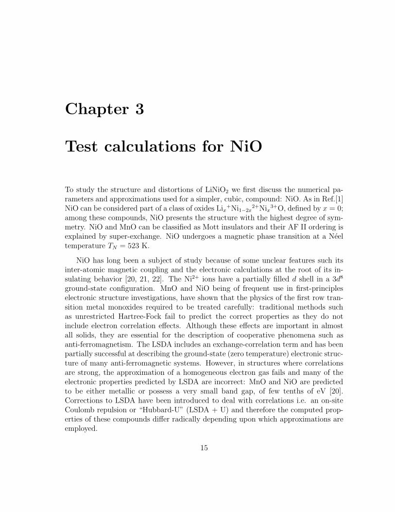
Figure 3.1: NiO cubic (rocksalt) structure. Nickel ions are represented by small bluespheres and oxygen ions by large gray spheres.
3.1 Structure of NiO
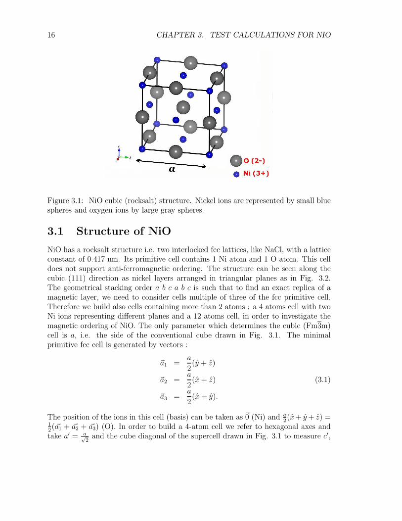
NiO has a rocksalt structure i.e. two interlocked fcc lattices, like NaCl, with a latticeconstant of 0.417 nm. Its primitive cell contains 1 Ni atom and 1 O atom. This celldoes not support anti-ferromagnetic ordering. The structure can be seen along thecubic (111) direction as nickel layers arranged in triangular planes as in Fig. 3.2.The geometrical stacking order a b c a b c is such that to find an exact replica of amagnetic layer, we need to consider cells multiple of three of the fcc primitive cell.Therefore we build also cells containing more than 2 atoms : a 4 atoms cell with twoNi ions representing different planes and a 12 atoms cell, in order to investigate themagnetic ordering of NiO. The only parameter which determines the cubic (Fm3m)cell is a, i.e. the side of the conventional cube drawn in Fig. 3.1. The minimalprimitive fcc cell is generated by vectors :
~a1 =a
2(y + z)
~a2 =a
2(x+ z) (3.1)
~a3 =a
2(x+ y).
The position of the ions in this cell (basis) can be taken as ~0 (Ni) and a2(x+ y+ z) =
1
2(~a1 + ~a2 + ~a3) (O). In order to build a 4-atom cell we refer to hexagonal axes and
take a′ = a√2
and the cube diagonal of the supercell drawn in Fig. 3.1 to measure c′,
3.1. STRUCTURE OF NIO 17
x’
y’
(a)
(b) (c)
Figure 3.2: The geometry of NiO seen as a stacking of triangular planes along thecubic (111) direction. Ni ions are represented as small blue spheres and O ions in asspheres of different shades of gray as they belong to two different triangular planes.(a) The stacking a b c a b c of the triangular planes seen along the cubic (111)direction. (b) A side view of the stacking of a Ni plane and 2 oxygen planes withthe Ni-Ni and O-O links highlighted, so that it is apparent that each Ni atom issurrounded by an octahedron of 6 oxygens. (c) The same stacking of planes, withthe Ni-O bonds highlighted.
18 CHAPTER 3. TEST CALCULATIONS FOR NIO
thus c′=√
6a′=√
3a. The primitive vectors are then:
~a′1 = a′x′
~a′2 = −a′
2x′ +
√3a′
2y′ (3.2)
~a′3 =a′√3y′ +
c′
6z′.
in a rotated reference frame
x′ = − x√2
+y√2
y′ = − x√6− y√
6+
√2√3z′
z′ =x√3
+y√3
+z√3
(3.3)
and the atomic positions in Cartesian coordinates (in the same reference frame) are:
Ni1 = ~0
O1 =a′√3y +
c′
6z =
1
4~a′1 +
1
2~a′2 +
1
4~a′3
Ni2 =a′
2x+
a′
2√
3y +
c′
3z =
1
2~a′1 +
1
2~a′3 (3.4)
O2 =c′
2z = −1
4~a′1 −
1
2~a′2 +
3
4~a′3.
3.2 Convergency calculations
3.2.1 Convergence with respect to Ecutoff
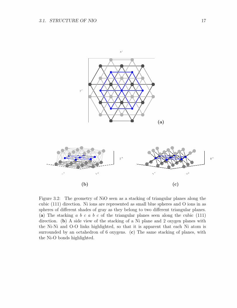
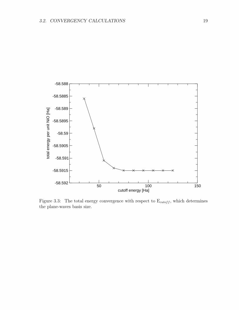
As the Ecutoff determines the number of elements of the plane-waves basis set neededto describe the system. This in turn determines the computational cost of the calcula-tions. We perform a convergence test over this parameter. The calculations reportedin Fig. 3.3 show that the total energy depends very weakly on Ecutoff above about50 Ha. We then take Ecutoff=55 Ha.
3.2. CONVERGENCY CALCULATIONS 19
50 100 150cutoff energy [Ha]
-58.592
-58.5915
-58.591
-58.5905
-58.59
-58.5895
-58.589
-58.5885
-58.588
tota
l ene
rgy
per
unit
NiO
[Ha]
Figure 3.3: The total energy convergence with respect to Ecutoff , which determinesthe plane-waves basis size.
20 CHAPTER 3. TEST CALCULATIONS FOR NIO
0 50 100 150 200density of k-points [Bohr^3]
-58.5908
-58.5907
-58.5906
-58.5905
-58.5904
-58.5903
-58.5902
tota
l ene
rgy
per
unit
form
ula
NiO
[H
a]
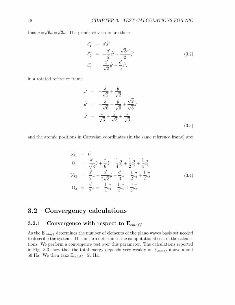
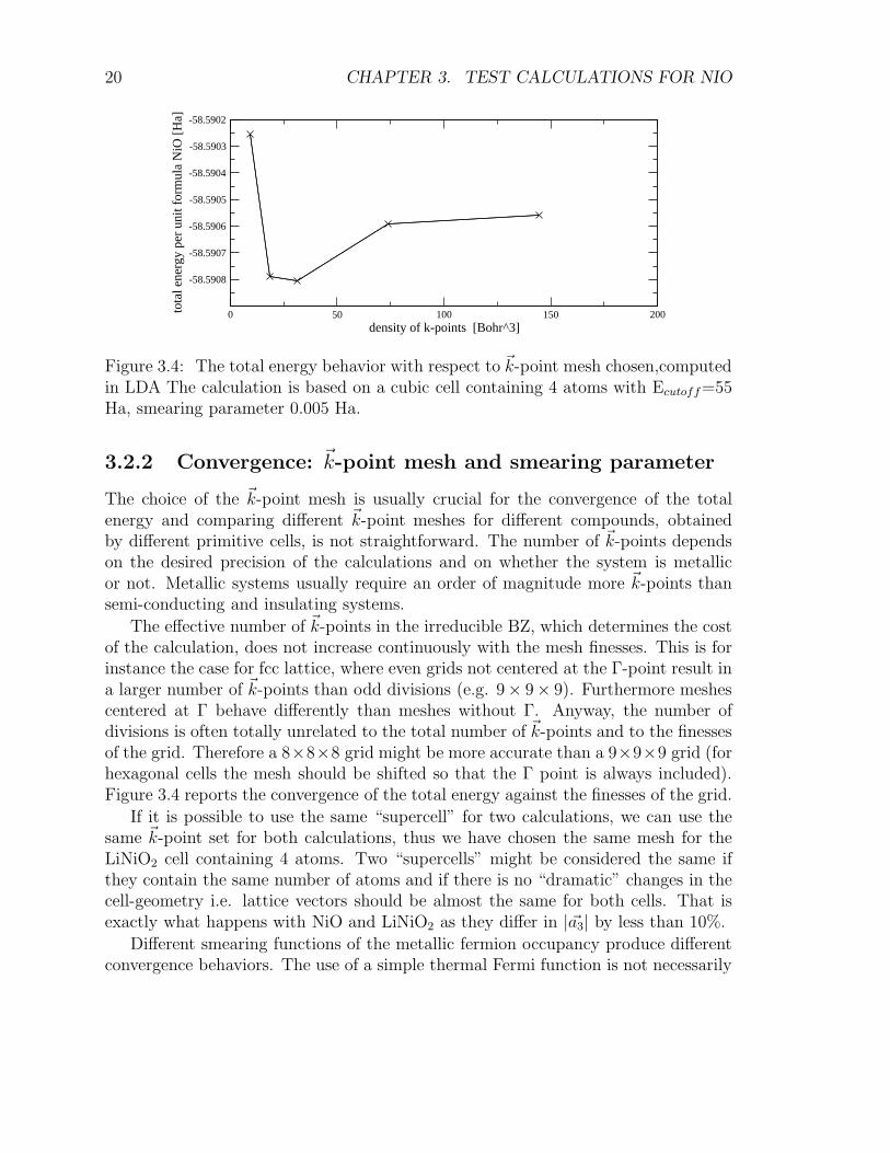
Figure 3.4: The total energy behavior with respect to ~k-point mesh chosen,computedin LDA The calculation is based on a cubic cell containing 4 atoms with Ecutoff=55Ha, smearing parameter 0.005 Ha.
3.2.2 Convergence: ~k-point mesh and smearing parameter
The choice of the ~k-point mesh is usually crucial for the convergence of the totalenergy and comparing different ~k-point meshes for different compounds, obtainedby different primitive cells, is not straightforward. The number of ~k-points dependson the desired precision of the calculations and on whether the system is metallicor not. Metallic systems usually require an order of magnitude more ~k-points thansemi-conducting and insulating systems.
The effective number of ~k-points in the irreducible BZ, which determines the costof the calculation, does not increase continuously with the mesh finesses. This is forinstance the case for fcc lattice, where even grids not centered at the Γ-point result ina larger number of ~k-points than odd divisions (e.g. 9× 9× 9). Furthermore meshescentered at Γ behave differently than meshes without Γ. Anyway, the number ofdivisions is often totally unrelated to the total number of ~k-points and to the finessesof the grid. Therefore a 8×8×8 grid might be more accurate than a 9×9×9 grid (forhexagonal cells the mesh should be shifted so that the Γ point is always included).Figure 3.4 reports the convergence of the total energy against the finesses of the grid.
If it is possible to use the same “supercell” for two calculations, we can use thesame ~k-point set for both calculations, thus we have chosen the same mesh for theLiNiO2 cell containing 4 atoms. Two “supercells” might be considered the same ifthey contain the same number of atoms and if there is no “dramatic” changes in thecell-geometry i.e. lattice vectors should be almost the same for both cells. That isexactly what happens with NiO and LiNiO2 as they differ in |~a3| by less than 10%.
Different smearing functions of the metallic fermion occupancy produce differentconvergence behaviors. The use of a simple thermal Fermi function is not necessarily
3.3. THE NIO LATTICE PARAMETER 21
0 0.005 0.01 0.015 0.02smearing [Ha]
-58.5905
-58.59
-58.5895
-58.589
-58.5885
-58.588
-58.5875
tota
l ene
rgy
per
unit
form
ula
NiO
[H
a]
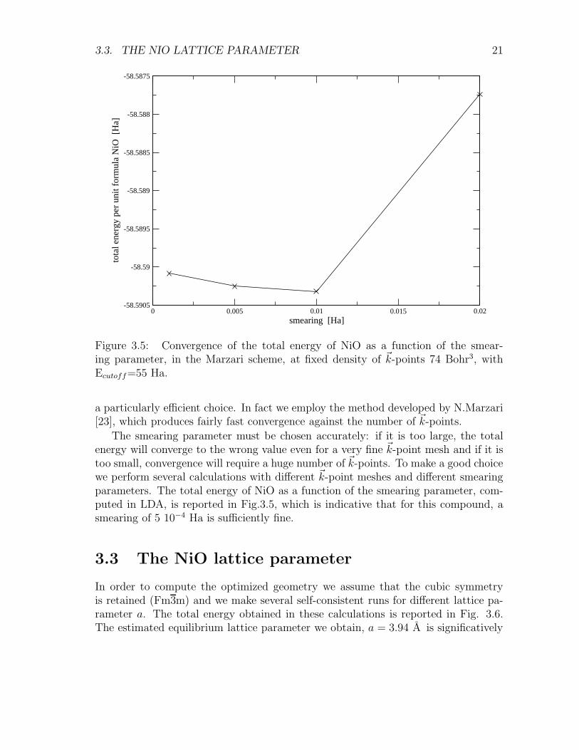
Figure 3.5: Convergence of the total energy of NiO as a function of the smear-ing parameter, in the Marzari scheme, at fixed density of ~k-points 74 Bohr3, withEcutoff=55 Ha.
a particularly efficient choice. In fact we employ the method developed by N.Marzari[23], which produces fairly fast convergence against the number of ~k-points.
The smearing parameter must be chosen accurately: if it is too large, the totalenergy will converge to the wrong value even for a very fine ~k-point mesh and if it istoo small, convergence will require a huge number of ~k-points. To make a good choicewe perform several calculations with different ~k-point meshes and different smearingparameters. The total energy of NiO as a function of the smearing parameter, com-puted in LDA, is reported in Fig.3.5, which is indicative that for this compound, asmearing of 5 10−4 Ha is sufficiently fine.
3.3 The NiO lattice parameter
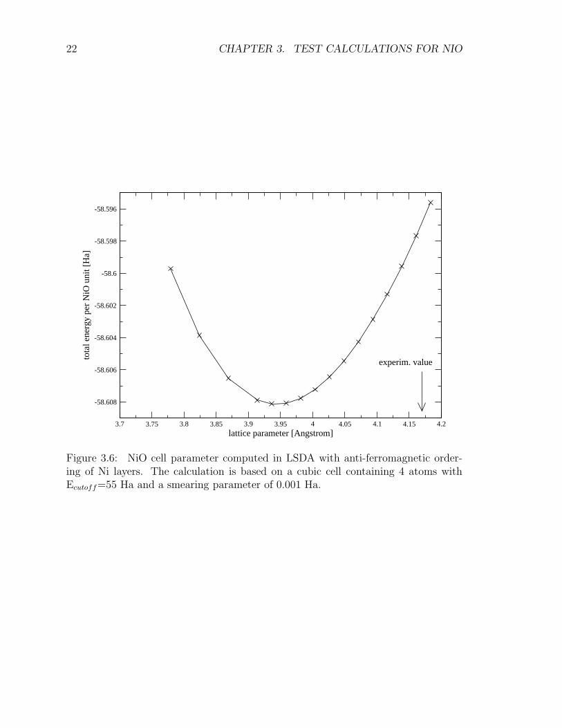
In order to compute the optimized geometry we assume that the cubic symmetryis retained (Fm3m) and we make several self-consistent runs for different lattice pa-rameter a. The total energy obtained in these calculations is reported in Fig. 3.6.The estimated equilibrium lattice parameter we obtain, a = 3.94 A is significatively
22 CHAPTER 3. TEST CALCULATIONS FOR NIO
3.7 3.75 3.8 3.85 3.9 3.95 4 4.05 4.1 4.15 4.2lattice parameter [Angstrom]
-58.608
-58.606
-58.604
-58.602
-58.6
-58.598
-58.596
tota
l ene
rgy
per
NiO
uni
t [H
a]
experim. value
Figure 3.6: NiO cell parameter computed in LSDA with anti-ferromagnetic order-ing of Ni layers. The calculation is based on a cubic cell containing 4 atoms withEcutoff=55 Ha and a smearing parameter of 0.001 Ha.
3.4. NIO BAND STRUCTURE AND MAGNETIC ORDERING 23
smaller than the experimentally observed one of 4.17 AAs discussed in Ref. [20]this is likely to be due to inadequacies of the LSDA to describe the strong Coulombrepulsion between 3d electrons of Ni2+ ions.
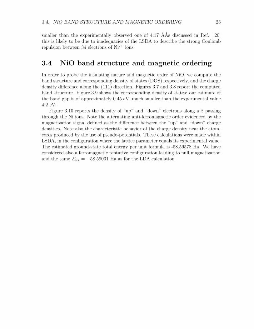
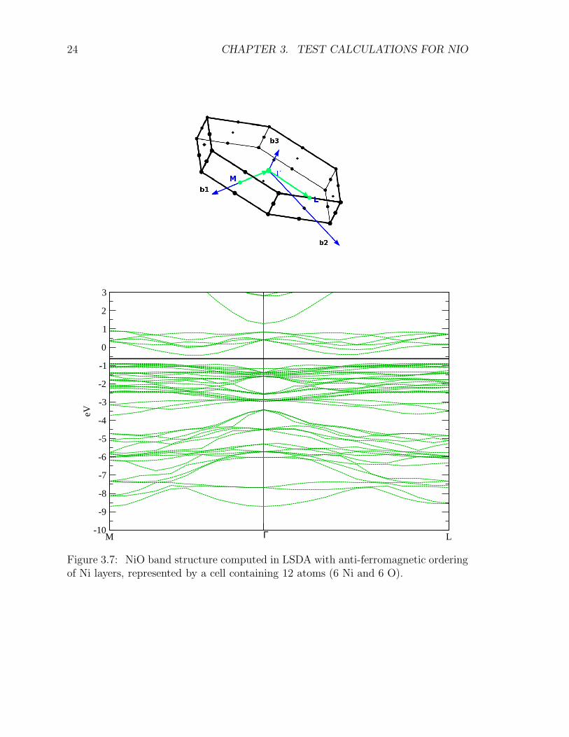
3.4 NiO band structure and magnetic ordering
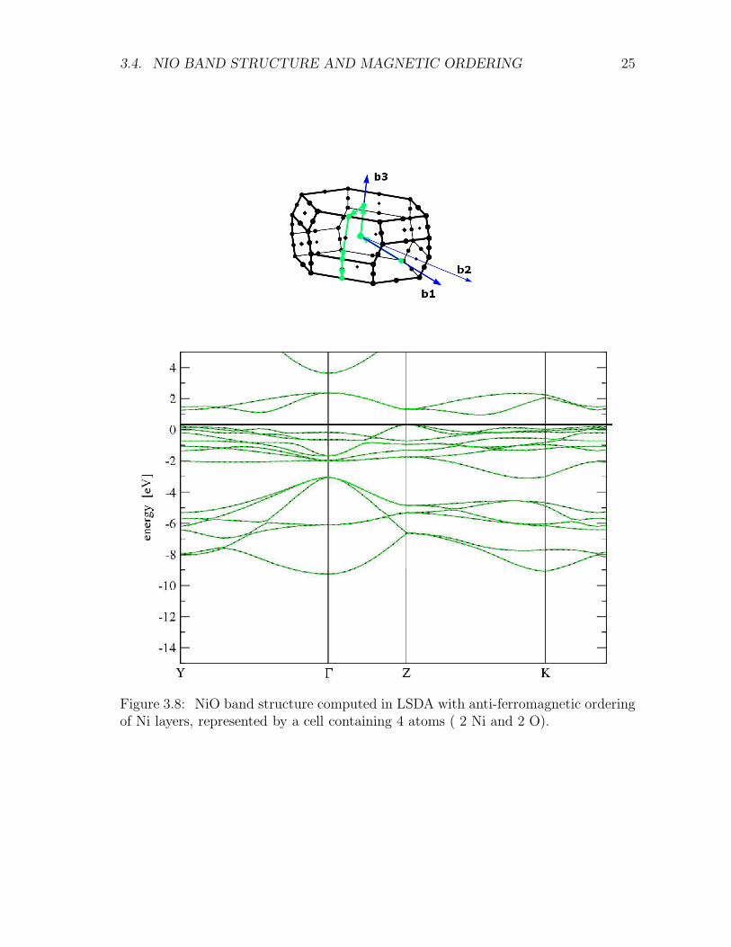
In order to probe the insulating nature and magnetic order of NiO, we compute theband structure and corresponding density of states (DOS) respectively, and the chargedensity difference along the (111) direction. Figures 3.7 and 3.8 report the computedband structure. Figure 3.9 shows the corresponding density of states: our estimate ofthe band gap is of approximately 0.45 eV, much smaller than the experimental value4.2 eV.
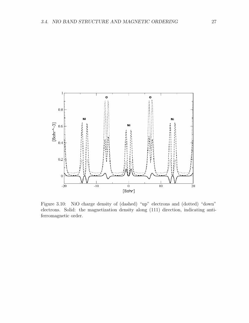
Figure 3.10 reports the density of “up” and “down” electrons along a z passingthrough the Ni ions. Note the alternating anti-ferromagnetic order evidenced by themagnetization signal defined as the difference between the “up” and “down” chargedensities. Note also the characteristic behavior of the charge density near the atom-cores produced by the use of pseudo-potentials. These calculations were made withinLSDA, in the configuration where the lattice parameter equals its experimental value.The estimated ground-state total energy per unit formula is -58.59578 Ha. We haveconsidered also a ferromagnetic tentative configuration leading to null magnetizationand the same Etot = −58.59031 Ha as for the LDA calculation.
24 CHAPTER 3. TEST CALCULATIONS FOR NIO
M L-10
-9
-8
-7
-6
-5
-4
-3
-2
-1
0
1
2
3
eV
Γ
Figure 3.7: NiO band structure computed in LSDA with anti-ferromagnetic orderingof Ni layers, represented by a cell containing 12 atoms (6 Ni and 6 O).
3.4. NIO BAND STRUCTURE AND MAGNETIC ORDERING 25
Figure 3.8: NiO band structure computed in LSDA with anti-ferromagnetic orderingof Ni layers, represented by a cell containing 4 atoms ( 2 Ni and 2 O).
26 CHAPTER 3. TEST CALCULATIONS FOR NIO
-0.1 -0.08 -0.06 -0.04 -0.02 0 0.02 0.04 0.06 0.08 0.1energy [Ha]
0
100
200
300
400
elec
tron
s/H
artr
ee/c
ell
LSDA antiferro
DOS NiO 4 atoms cell
ecut 55 Ha tsmear
Figure 3.9: NiO electronic DOS, computed in LSDA with anti-ferromagnetic orderingof Ni layers. As in all calculations, we take Ecutoff=55 Ha and occupancy smearingof 0.005 Ha.
3.4. NIO BAND STRUCTURE AND MAGNETIC ORDERING 27
Figure 3.10: NiO charge density of (dashed) “up” electrons and (dotted) “down”electrons. Solid: the magnetization density along (111) direction, indicating anti-ferromagnetic order.

28 CHAPTER 3. TEST CALCULATIONS FOR NIO
Chapter 4
LiNiO2
4.1 Structure and system energetics
According to Ref.[1], the class of oxides Li1−x Ni1+xO (x runs from 0 to 1) crystallizesapproximately with the cubic rock-salt structure of NiO (Fig. 1.1). The side of thecubic cell decreases with increasing x, thus with increasing fraction of the smaller Li+
and Ni3+ ions.
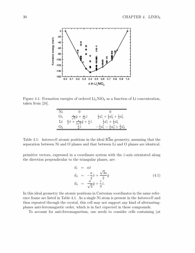
Figure 3.2 can be used also to visualize the structure of LiNiO2: Ni3+, O2− andLi+ planes alternate along the (111) direction (each plane ordered in a perfect tri-angular lattice) with nickel ions caged within edge-sharing octahedra of oxygen ions.This configuration is highly idealized, as real Li1−x Ni1+xO is strongly disordered andpoorly stoichiometric. Different composition show different thermodynamical stabil-ity as shown in Fig. 4.1. Experimentally, the Li0.98Ni1.02O2 compound is the closestto ideal stoichiometric LiNiO2.
X-rays measurements show a rhombohedral R3m structure characterized by latticeparameters a = 2.878 A and c = 14.19 A [1]. a represents the side of the equilateraltriangles of, e.g., Ni atoms; c represents the distance between two successive layers ofNi that are stacked exactly above each other: thus c equals three times the distancebetween successive layers of Ni, as shown in Fig. 4.2. In terms of the geometry ofFig. 1.1, the distance c is measured along the (111) direction, i.e. along the cubediagonal. This same ideal geometry is represented in Fig.4.2 with c in the uprightdirection. Based on these parameters, it is possible to construct several different unitcells, which, once repeated periodically to fill the whole space, produce the same idealcrystal structure.
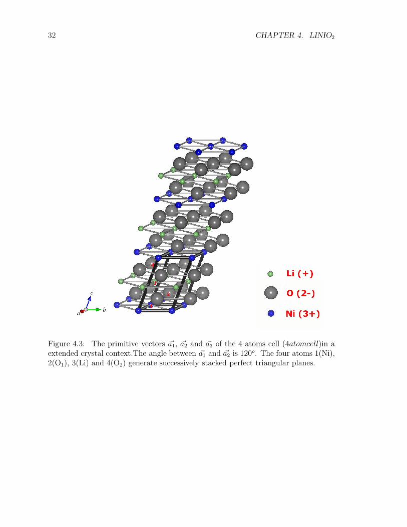
The most “economical” of these cells contains only 4 atoms as in the unit formulaLiNiO2. Each atom belongs to a different triangular plane. This geometric arrange-ment, identified as “4atomcell” , is illustrated in Fig. 4.3. The length of both ~a1 and
~a2 primitive vectors equals a, and |~a3| =√
a2
3+ c2
9. The Cartesian coordinates of the
29
30 CHAPTER 4. LINIO2
Figure 4.1: Formation energies of ordered LixNiO2 as a function of Li concentration,taken from [24].
Ni 0 0O1
a√3y + c
12z 1
4~a1 + 1
2~a2 + 1
4~a3
Li a2x+ a
2√
3y + c
6z 1
2~a1 + 1
2~a3
O2c4z −1
4~a1 − 1
2a~2 + 3
4~a3
Table 4.1: 4atomcell atomic positions in the ideal R3m geometry, assuming that theseparation between Ni and O planes and that between Li and O planes are identical.
primitive vectors, expressed in a coordinate system with the z-axis orientated alongthe direction perpendicular to the triangular planes, are:
~a1 = ax
~a2 = −a2x+
√3a
2y (4.1)
~a3 =a√3y +
c
3z.
In this ideal geometry the atomic positions in Cartesian coordinates in the same refer-ence frame are listed in Table 4.1. As a single Ni atom is present in the 4atomcell andthen repeated through the crystal, this cell may not support any kind of alternating-planes anti-ferromagnetic order, which is in fact expected in these compounds.
To account for anti-ferromagnetism, one needs to consider cells containing (at
4.1. STRUCTURE AND SYSTEM ENERGETICS 31
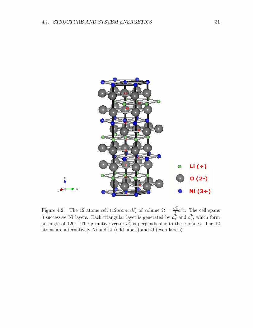
Figure 4.2: The 12 atoms cell (12atomcell) of volume Ω =√
3
2a2c. The cell spans
3 successive Ni layers. Each triangular layer is generated by ~a′′1 and ~a′′2, which form
an angle of 120o. The primitive vector ~a′′3 is perpendicular to these planes. The 12atoms are alternatively Ni and Li (odd labels) and O (even labels).
32 CHAPTER 4. LINIO2
Figure 4.3: The primitive vectors ~a1, ~a2 and ~a3 of the 4 atoms cell (4atomcell)in aextended crystal context.The angle between ~a1 and ~a2 is 120o. The four atoms 1(Ni),2(O1), 3(Li) and 4(O2) generate successively stacked perfect triangular planes.
4.1. STRUCTURE AND SYSTEM ENERGETICS 33
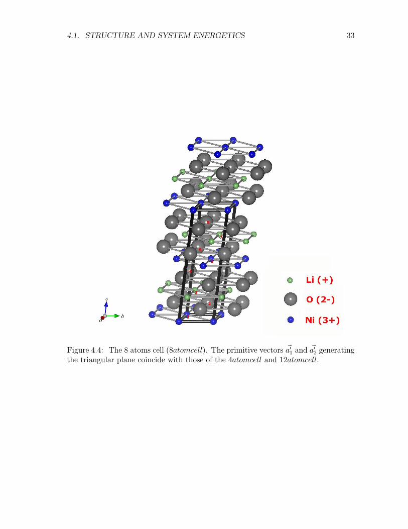
Figure 4.4: The 8 atoms cell (8atomcell). The primitive vectors ~a′1 and ~a′2 generatingthe triangular plane coincide with those of the 4atomcell and 12atomcell.
34 CHAPTER 4. LINIO2
Ni1 0 0
O1a√3y + c
12z 1
4~a′1 + 3
8~a′2 + 1
8~a′3
Li1a2x+ a
2√
3y + c
6z 1
2~a′1 + 1
4~a′2 + 1
4~a′3
O2c4z −1
4~a′1 − 1
8~a′2 + 3
8~a′3
Ni2a√3y + c
3z 1
2~a′2 + 1
2~a′3
O3a2x+ a
2√
3y + 5c
12z 1
4~a′1 + 1
8~a′2 + 5
8~a′3
Li2c2z −1
2~a′1 − 1
4~a′2 + 3
4~a′3
O4 ax+ a√3y + 7c
12z 3
4~a′1 + 3
8~a′2 + 7
8~a′3
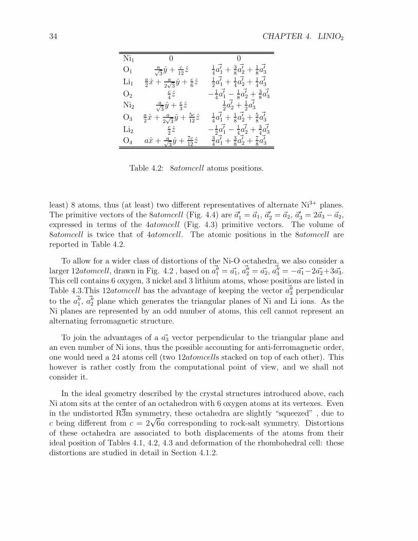
Table 4.2: 8atomcell atoms positions.
least) 8 atoms, thus (at least) two different representatives of alternate Ni3+ planes.The primitive vectors of the 8atomcell (Fig. 4.4) are ~a′1 = ~a1, ~a
′2 = ~a2, ~a
′3 = 2~a3 −~a2,
expressed in terms of the 4atomcell (Fig. 4.3) primitive vectors. The volume of8atomcell is twice that of 4atomcell. The atomic positions in the 8atomcell arereported in Table 4.2.
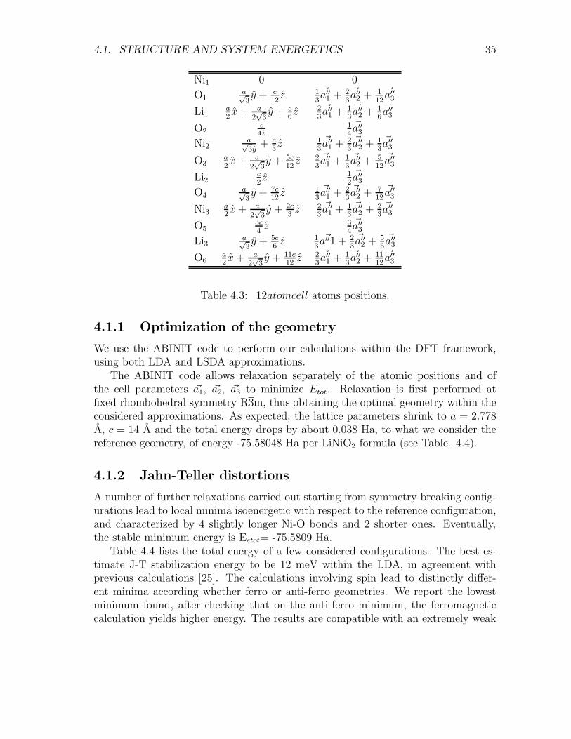
To allow for a wider class of distortions of the Ni-O octahedra, we also consider alarger 12atomcell, drawn in Fig. 4.2 , based on ~a′′1 = ~a1, ~a
′′2 = ~a2, ~a
′′3 = −~a1−2~a2+3~a3.
This cell contains 6 oxygen, 3 nickel and 3 lithium atoms, whose positions are listed inTable 4.3.This 12atomcell has the advantage of keeping the vector ~a′′3 perpendicular
to the ~a′′1,~a′′2 plane which generates the triangular planes of Ni and Li ions. As the
Ni planes are represented by an odd number of atoms, this cell cannot represent analternating ferromagnetic structure.
To join the advantages of a ~a3 vector perpendicular to the triangular plane andan even number of Ni ions, thus the possible accounting for anti-ferromagnetic order,one would need a 24 atoms cell (two 12atomcells stacked on top of each other). Thishowever is rather costly from the computational point of view, and we shall notconsider it.
In the ideal geometry described by the crystal structures introduced above, eachNi atom sits at the center of an octahedron with 6 oxygen atoms at its vertexes. Evenin the undistorted R3m symmetry, these octahedra are slightly “squeezed” , due toc being different from c = 2
√6a corresponding to rock-salt symmetry. Distortions
of these octahedra are associated to both displacements of the atoms from theirideal position of Tables 4.1, 4.2, 4.3 and deformation of the rhombohedral cell: thesedistortions are studied in detail in Section 4.1.2.
4.1. STRUCTURE AND SYSTEM ENERGETICS 35
Ni1 0 0
O1a√3y + c
12z 1
3~a′′1 + 2
3~a′′2 + 1
12~a′′3
Li1a2x+ a
2√
3y + c
6z 2
3~a′′1 + 1
3~a′′2 + 1
6~a′′3
O2c4z
1
4~a′′3
Ni2a√3y
+ c3z 1
3~a′′1 + 2
3~a′′2 + 1
3~a′′3
O3a2x+ a
2√
3y + 5c
12z 2
3~a′′1 + 1
3~a′′2 + 5
12~a′′3
Li2c2z 1
2~a′′3
O4a√3y + 7c
12z 1
3~a′′1 + 2
3~a′′2 + 7
12~a′′3
Ni3a2x+ a
2√
3y + 2c
3z 2
3~a′′1 + 1
3~a′′2 + 2
3~a′′3
O53c4z 3
4~a′′3
Li3a√3y + 5c
6z 1
3~a′′1 + 2
3~a′′2 + 5
6~a′′3
O6a2x+ a
2√
3y + 11c
12z 2
3~a′′1 + 1
3~a′′2 + 11
12~a′′3
Table 4.3: 12atomcell atoms positions.
4.1.1 Optimization of the geometry
We use the ABINIT code to perform our calculations within the DFT framework,using both LDA and LSDA approximations.
The ABINIT code allows relaxation separately of the atomic positions and ofthe cell parameters ~a1, ~a2, ~a3 to minimize Etot. Relaxation is first performed atfixed rhombohedral symmetry R3m, thus obtaining the optimal geometry within theconsidered approximations. As expected, the lattice parameters shrink to a = 2.778A, c = 14 A and the total energy drops by about 0.038 Ha, to what we consider thereference geometry, of energy -75.58048 Ha per LiNiO2 formula (see Table. 4.4).
4.1.2 Jahn-Teller distortions
A number of further relaxations carried out starting from symmetry breaking config-urations lead to local minima isoenergetic with respect to the reference configuration,and characterized by 4 slightly longer Ni-O bonds and 2 shorter ones. Eventually,the stable minimum energy is Eetot= -75.5809 Ha.
Table 4.4 lists the total energy of a few considered configurations. The best es-timate J-T stabilization energy to be 12 meV within the LDA, in agreement withprevious calculations [25]. The calculations involving spin lead to distinctly differ-ent minima according whether ferro or anti-ferro geometries. We report the lowestminimum found, after checking that on the anti-ferro minimum, the ferromagneticcalculation yields higher energy. The results are compatible with an extremely weak
36 CHAPTER 4. LINIO2
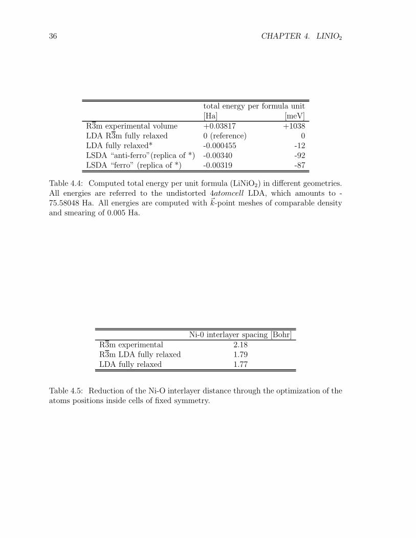
total energy per formula unit[Ha] [meV]
R3m experimental volume +0.03817 +1038LDA R3m fully relaxed 0 (reference) 0LDA fully relaxed* -0.000455 -12LSDA “anti-ferro”(replica of *) -0.00340 -92LSDA “ferro” (replica of *) -0.00319 -87
Table 4.4: Computed total energy per unit formula (LiNiO2) in different geometries.All energies are referred to the undistorted 4atomcell LDA, which amounts to -75.58048 Ha. All energies are computed with ~k-point meshes of comparable densityand smearing of 0.005 Ha.
Ni-0 interlayer spacing [Bohr]R3m experimental 2.18R3m LDA fully relaxed 1.79LDA fully relaxed 1.77
Table 4.5: Reduction of the Ni-O interlayer distance through the optimization of theatoms positions inside cells of fixed symmetry.
4.1. STRUCTURE AND SYSTEM ENERGETICS 37
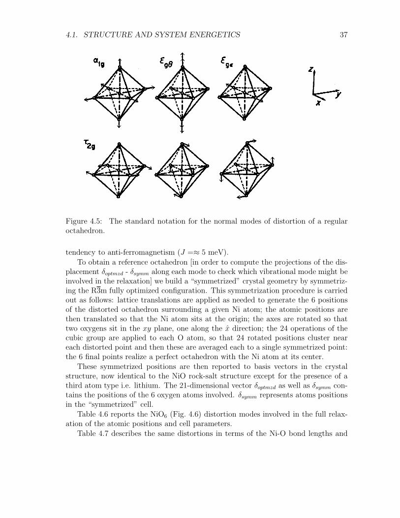
Figure 4.5: The standard notation for the normal modes of distortion of a regularoctahedron.
tendency to anti-ferromagnetism (J =≈ 5 meV).
To obtain a reference octahedron [in order to compute the projections of the dis-placement δoptmzd - δsymm along each mode to check which vibrational mode might beinvolved in the relaxation] we build a “symmetrized” crystal geometry by symmetriz-ing the R3m fully optimized configuration. This symmetrization procedure is carriedout as follows: lattice translations are applied as needed to generate the 6 positionsof the distorted octahedron surrounding a given Ni atom; the atomic positions arethen translated so that the Ni atom sits at the origin; the axes are rotated so thattwo oxygens sit in the xy plane, one along the x direction; the 24 operations of thecubic group are applied to each O atom, so that 24 rotated positions cluster neareach distorted point and then these are averaged each to a single symmetrized point:the 6 final points realize a perfect octahedron with the Ni atom at its center.
These symmetrized positions are then reported to basis vectors in the crystalstructure, now identical to the NiO rock-salt structure except for the presence of athird atom type i.e. lithium. The 21-dimensional vector δoptmzd as well as δsymm con-tains the positions of the 6 oxygen atoms involved. δsymm represents atoms positionsin the “symmetrized” cell.
Table 4.6 reports the NiO6 (Fig. 4.6) distortion modes involved in the full relax-ation of the atomic positions and cell parameters.
Table 4.7 describes the same distortions in terms of the Ni-O bond lengths and
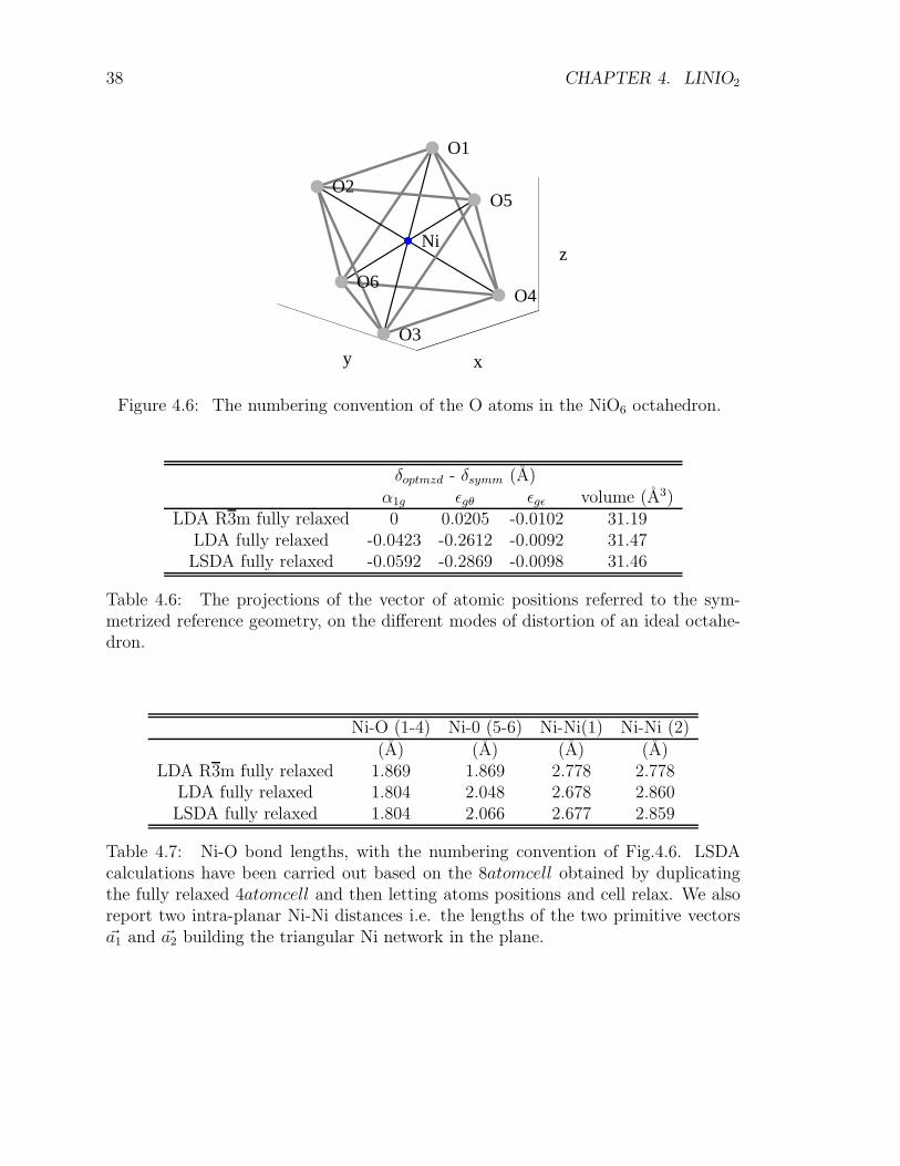
38 CHAPTER 4. LINIO2
xy
zNi
O1
O2
O3
O4
O5
O6
x
Figure 4.6: The numbering convention of the O atoms in the NiO6 octahedron.
δoptmzd - δsymm (A)α1g ǫgθ ǫgǫ volume (A3)
LDA R3m fully relaxed 0 0.0205 -0.0102 31.19LDA fully relaxed -0.0423 -0.2612 -0.0092 31.47LSDA fully relaxed -0.0592 -0.2869 -0.0098 31.46
Table 4.6: The projections of the vector of atomic positions referred to the sym-metrized reference geometry, on the different modes of distortion of an ideal octahe-dron.
Ni-O (1-4) Ni-0 (5-6) Ni-Ni(1) Ni-Ni (2)
(A) (A) (A) (A)LDA R3m fully relaxed 1.869 1.869 2.778 2.778
LDA fully relaxed 1.804 2.048 2.678 2.860LSDA fully relaxed 1.804 2.066 2.677 2.859
Table 4.7: Ni-O bond lengths, with the numbering convention of Fig.4.6. LSDAcalculations have been carried out based on the 8atomcell obtained by duplicatingthe fully relaxed 4atomcell and then letting atoms positions and cell relax. We alsoreport two intra-planar Ni-Ni distances i.e. the lengths of the two primitive vectors~a1 and ~a2 building the triangular Ni network in the plane.
4.2. BANDS 39
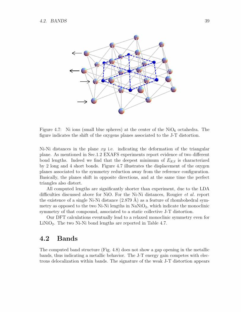
Figure 4.7: Ni ions (small blue spheres) at the center of the NiO6 octahedra. Thefigure indicates the shift of the oxygens planes associated to the J-T distortion.
Ni-Ni distances in the plane xy i.e. indicating the deformation of the triangularplane. As mentioned in Sec.1.2 EXAFS experiments report evidence of two differentbond lengths. Indeed we find that the deepest minimum of EKS is characterizedby 2 long and 4 short bonds. Figure 4.7 illustrates the displacement of the oxygenplanes associated to the symmetry reduction away from the reference configuration.Basically, the planes shift in opposite directions, and at the same time the perfecttriangles also distort.
All computed lengths are significantly shorter than experiment, due to the LDAdifficulties discussed above for NiO. For the Ni-Ni distances, Rougier et al . reportthe existence of a single Ni-Ni distance (2.879 A) as a feature of rhombohedral sym-metry as opposed to the two Ni-Ni lengths in NaNiO2, which indicate the monoclinicsymmetry of that compound, associated to a static collective J-T distortion.
Our DFT calculations eventually lead to a relaxed monoclinic symmetry even forLiNiO2. The two Ni-Ni bond lengths are reported in Table 4.7.
4.2 Bands
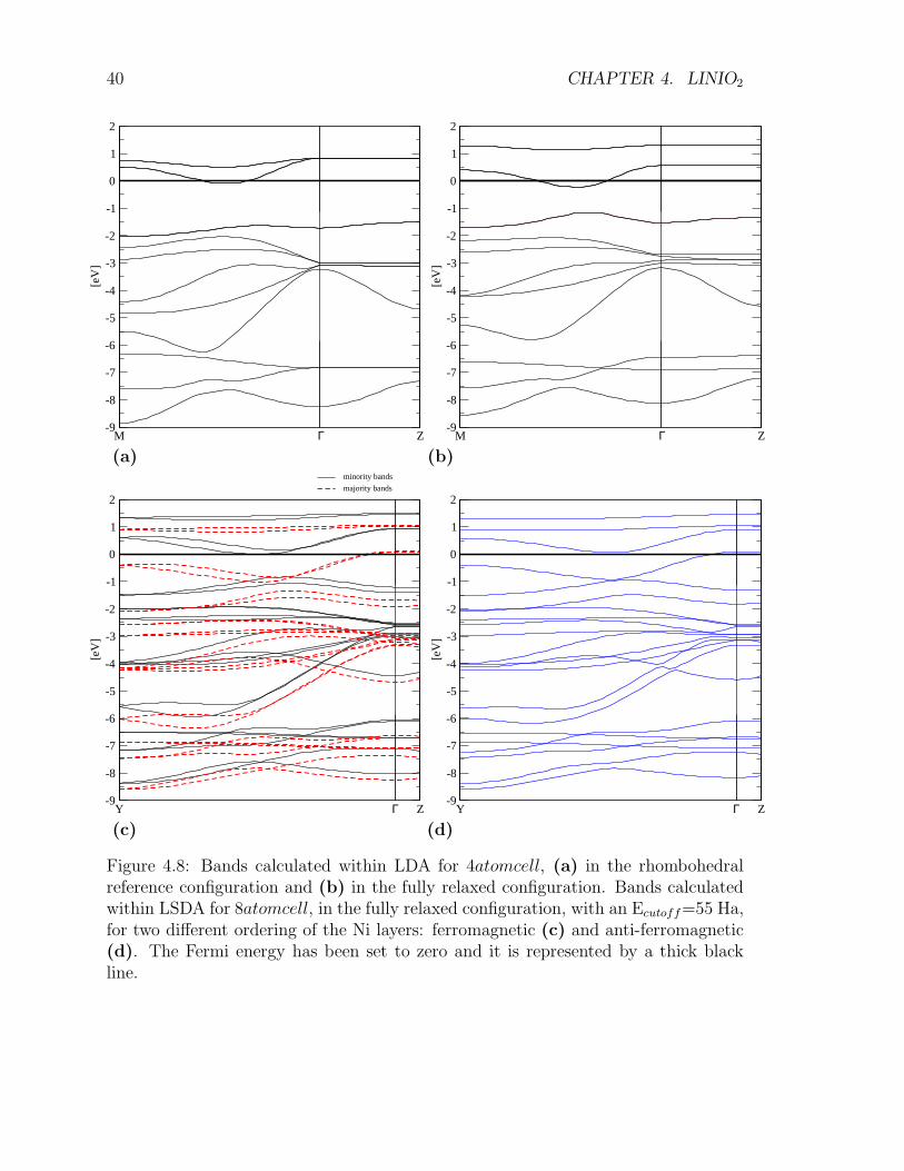
The computed band structure (Fig. 4.8) does not show a gap opening in the metallicbands, thus indicating a metallic behavior. The J-T energy gain competes with elec-trons delocalization within bands. The signature of the weak J-T distortion appears
40 CHAPTER 4. LINIO2
M Γ Z-9
-8
-7
-6
-5
-4
-3
-2
-1
0
1
2
[eV
]
M Γ Z-9
-8
-7
-6
-5
-4
-3
-2
-1
0
1
2
[eV
]
(a) (b)
Y Γ Z-9
-8
-7
-6
-5
-4
-3
-2
-1
0
1
2
[eV
]
minority bands
majority bands
Y Γ Z-9
-8
-7
-6
-5
-4
-3
-2
-1
0
1
2
[eV
]
(c) (d)
Figure 4.8: Bands calculated within LDA for 4atomcell, (a) in the rhombohedralreference configuration and (b) in the fully relaxed configuration. Bands calculatedwithin LSDA for 8atomcell, in the fully relaxed configuration, with an Ecutoff=55 Ha,for two different ordering of the Ni layers: ferromagnetic (c) and anti-ferromagnetic(d). The Fermi energy has been set to zero and it is represented by a thick blackline.
4.2. BANDS 41
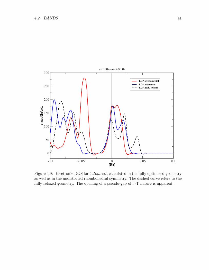
Figure 4.9: Electronic DOS for 4atomcell, calculated in the fully optimized geometryas well as in the undistorted rhombohedral symmetry. The dashed curve refers to thefully relaxed geometry. The opening of a pseudo-gap of J-T nature is apparent.
42 CHAPTER 4. LINIO2
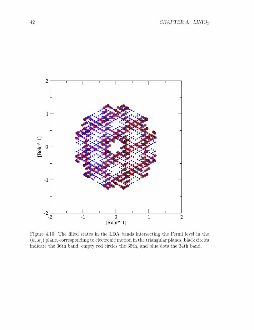
Figure 4.10: The filled states in the LDA bands intersecting the Fermi level in the(kx,ky) plane, corresponding to electronic motion in the triangular planes, black circlesindicate the 36th band, empty red circles the 35th, and blue dots the 34th band.
4.2. BANDS 43
-0.1 -0.05 0 0.05 0.1[Ha]
0
50
100
150
200
250
300
stat
es/H
a/ce
ll
LDA fully relaxedLSDA antiferroLSDA ferro spin downLSDA ferro spin up
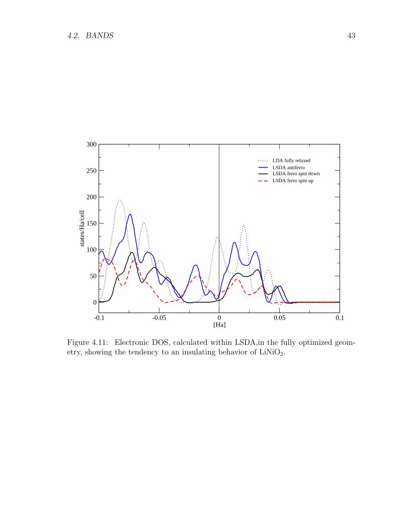
Figure 4.11: Electronic DOS, calculated within LSDA,in the fully optimized geom-etry, showing the tendency to an insulating behavior of LiNiO2.
44 CHAPTER 4. LINIO2
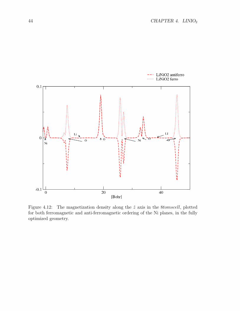
Figure 4.12: The magnetization density along the z axis in the 8tomscell, plottedfor both ferromagnetic and anti-ferromagnetic ordering of the Ni planes, in the fullyoptimized geometry.
4.2. BANDS 45
as splitting of about 1 eV of the eg-derived band at Γ, evident in the comparison ofFig.4.8 (a) and (b) . Correspondingly, a pseudo-gap deepens in the DOS in Fig. 4.9.The topology of the threefold Fermi surface is rather involved (Fig. 4.10).
LSDA computation in the fully distorted geometry lead to an estimate of theinter-planar exchange-correlation energy of approximately 5 meV. Computations inthe fully relaxed 8atomcell suggest (Fig. 4.11 ) a tendency toward insulating behaviorin LiNiO2 where the anti-ferromagnetic ordering is slightly favored (see Fig. 4.12).

46 CHAPTER 4. LINIO2
Chapter 5
Conclusions and discussion
The present work reports a very preliminary analysis of the structure and distortionsof ideal stoichiometric crystalline LiNiO2. The calculations are carried out based onthe adiabatic scheme, and ab-initio DFT-LDA description for the electronic motion.Our results are consistent with the observed weak tendency of LiNiO2 to distort awayfrom the ideal rhombohedral symmetry, to a lower symmetry, which is generallyassumed to be monoclinic. In fact, our calculations find an even lower symmetry,involving distortions of the triangular planes away from perfect equilateral geometry.
The energy gain associated to the rhombohedral to distorted relaxation is, even-tually, very small, ≈ 12 meV, at the border of resolution of the approximate methodinvolved.This result is in good agreement with GGA calculations performed in [25].Part of this energy lowering is surely related to the relaxation to a C2/m monoclinicgeometry. The relevant bands at the Fermi level are found rather narrow (≈ 0.8 eVof total bandwidth). This bandwidth however is sufficient to hinder rather effectivelythe local tendency of the NiO6 octahedra to distort.
A collective sliding (of approximately ≈ 0.3 A) of the oxygen planes against themetal planes is expected. This displacement reflects in 2 different lengths of theNi-O bonds, with differences of the order ≈ 0.2 A, in good accord with EXAFSmeasurements. Full relaxation involves also distortions of the triangular lattice find-ing eventually two Ni-Ni distances, with differences of the same order. There is noexperimental observation of such distortion.
We must observe that the LDA is well known to underestimate the bond lengthsinvolving Ni atoms, due to the poor treatment of d electrons. Accordingly, the com-puted relaxed cell volume is ≈ 9% smaller than observed experimentally. This un-physical “compression” may play a significant role in inducing the extra distortionof the triangular planes. The generalized gradient approximation (GGA) is acknowl-edged to improve the treatment of d electrons, and could indeed find a better descrip-tion of the LiNiO2 relaxed geometry. We have not repeated the DFT calculationswith the GGA functional, for lack of time.
47
48 CHAPTER 5. CONCLUSIONS AND DISCUSSION
The present calculations involve only a small cell repeated periodically. Thisapproximation rules out the possibility of the richer patterns of distortions other thana rigid collective shifts of the oxygen planes, and the possibility to treat disorder andnon-stoichiometry, which is well known to play a significant role in this compound.We must be aware of other possible patterns of deformations, involving differentdistortions at different NiO6 octahedra. We have attempted calculations based onlarger (12 atoms) cells, but could not find any of this.
Our LSDA calculations provide also an estimate of the inter-planar exchangeenergy J ≈ 5 meV, favoring anti-ferromagnetic alignment of the spins of the nar-row (mainly Ni-d character) conduction band. Experimentally a tendency for anti-ferromagnetic fluctuations has been reported in, but no apparent long-range orderhas been found. The amount of defects (mainly Ni substitutions of Li ions) seemscrucial for the determination of the magnetic behavior : this substitution can intro-duce FM inter-planar coupling between Ni planes. Indeed , with low Ni impurityconcentration, the FM coupling is weak and LiNiO2 shows an AF (local) ordering asreported in [6, 26, 27].
The calculations at hand are very preliminary also at an adiabatic level. Dynami-cal effects are likely to play some role in a system where tunneling among weakly J-Tdistorted configurations separated by low energy barriers is a concrete possibility.
Bibliography
[1] Goodenough et al., J. Phys. Chem.Solids 5, 107 (1958).
[2] Rougier et al., Solid State Commun. 94, 123 (1995).
[3] A. Rougier, P. Gravereau and C. Delmas, J. Electrochem. Soc. 143, 1168 (1996).
[4] Y. Nitta et al., J.of Power Sources 68, 166 (1997).
[5] P. F. Bongers and U. Enz., J. Solid State Commun. 4, 153 (1966).
[6] J. Chung et al., Phys. Rev.B 71,064410 (2005).
[7] L. H. Thomas, Proc. Camb. Phil. Soc. 23, 542 (1927).
[8] E. Fermi, Rend. Accad., Lincei 6, 602 (1927).
[9] P. A. M. Dirac, Proc. Cambridge Philos. Soc. 26, 376 (1930).
[10] P. Hohenberg and W. Kohn, Phys. Rev.B 136, 864 (1964).
[11] ABINIT package at http://www.abinit.org .
[12] D. Chadi and M. Cohen, Phys. Rev.B 8, 5747 (1973).
[13] H. Monkhorst and J. Pack, Phys. Rev.B 13, 5188 (1976).
[14] A. Khein and D. C. Allan, http://www.abinit.org/Psps/LDA_TM/psp1.data .
[15] S. Goedecker, M. Teter, and J. Huetter, Phys. Rev.B 54, 1703 (1996).
[16] C. G. Broyden, Journal of the Institute for Mathematics and Applications 6,222 (1970).
[17] R. Fletcher, Computer Journal 13, 317 (1970).
[18] D. Goldfarb, Mathematics of Computation 24, 22 (1970).
49
50 BIBLIOGRAPHY
[19] D. F. Shanno, Mathematics of Computation 24, 647 (1970).
[20] S. L. Dudarev et al., Phys. Rev. B 57, 1505 (1998).
[21] K. Terakura et al., Phys. Rev.B 30, 4734 (1984).
[22] G. A. Sawatzky and J. W. Allen, Phys. Rev.Lett. 53, 418 (1984).
[23] N. Marzari, PhD dissertation, U.of Cambridge, http://nnn.mit.edu/phd/ ,(1996).
[24] M. E. Arroyo y de Dompablo et al., Phys. Rev. B 66, 064112 (2002).
[25] C. A. Marianetti, D. Morgan and G. Ceder, Phys. Rev.B 63, 224304 (2001).
[26] F. Reynaud et al., Eur. Phys. J. Appl. Phys. 18, 83 (2000).
[27] E. Chappel, PhD Thesis, Univ. J. Fourier Grenoble,http://tel.ccsd.cnrs.fr/documents/archives0/00/00/82/26/index.html ,(2000).
Ringraziamenti
Ringrazio per la pazienza, gli stimoli e l’incoraggiamento, in primo luogo NicolaManini.Per gli stessi motivi, i miei ringraziamenti vanno anche a Giovanni Onida, AndreaBordoni, a tutti quanti ”nel corridoio” mi abbiano aiutato e a Jeroen van den Brinkper la disponibilita dimostrata.Grazie (per mille ragioni) ai miei genitori, ad Andrea e ad Anzio.
51