Embed Size (px)
Citation preview

UNIVERSITA DEGLI STUDI DI VITERBO
DIPARTIMENTO DI SCIENZE ECOLOGICHE E BIOLOGICHE
Dottorato di Ricerca in Ecologia e Gestione delle Risorse Ecologiche
ciclo XXV
Marine data network of the Port Authority of Civitavecchia Fiumicino and
Gaeta: pilot project for oceanographic data sharing
BIO 07
Coordinatore
Prof. Giuseppe Nascetti
Tutor Candidato
Prof. Marco Marcelli Andrea Pannocchi
VITERBO MARZO, 2014
1

Indice generale
General Section 1 Introduction..................................................................................................................................... 7 2 Scientific context............................................................................................................................. 7 3 Oceanographic world data acquisition network and management programmes.............................8
3.1 International cooperation programme for data acquisition: (VOS SOOP, ARGO, Observatories, Satellites)............................................................................................................ 9 3.2 The WMO Voluntary Observing Ships (VOS) program..................................................... 9 3.3 The Ship-of-Opportunity Program (SOOP)...................................................................... 10
4 Worldwide oceanographic acquisition devices and platforms: the heterogeneity in data and meta data......................................................................................................................................................11
4.1 Platforms and sensors........................................................................................................11 4.1.1 Ships..................................................................................................................... 12 4.1.2 Moorings...............................................................................................................14 4.1.3 Underwater vehicles and lowered devices............................................................19 4.1.4 Lagrangian devices, expendable probes and drifter.............................................26
5 Oceanographic International Data sharing.................................................................................... 28 5.1 INSPIRE: INfrastructure for SPatial InfoRmation in the European Community............28
5.1.1 INSPIRE Directive aims.......................................................................................29 5.1.2 INSPIRE Coordination Team (CT).......................................................................29
5.1.2.1 DG Environment...................................................................................... 29 5.1.2.2 JRC........................................................................................................... 30 5.1.2.3 Eurostat.....................................................................................................30 5.1.2.4 EEA.......................................................................................................... 30 5.1.2.5 INSPIRE Committee (IC)........................................................................ 30 5.1.2.6 Member State Contact Points (MSCP).....................................................31 5.1.2.7 Initial Operating Capability Task Force (IOC TF)................................... 31
5.1.3 World web data services “INSPIRE COMPLIANT”...........................................31 5.1.3.1 The Open Geospatial Consortiums's role in Geosciences and the Environment. . .32 5.1.3.2 IODE Data Portal..................................................................................... 34 5.1.3.3 GEOSEVER............................................................................................. 35 5.1.3.4 U.S. IOOS®, Integrated Ocean Observing System.................................35 5.1.3.5 Australia Integrated Marine Observing System IMOS............................36 5.1.3.6 SEADATANET Pan European infrastructure for ocean and marine data management........................................................................................................... 36 5.1.3.7 GEO-SEAS...............................................................................................36 5.1.3.8 ODIP.........................................................................................................37
6 Pan-European infrastructures for ocean and marine data management: SEADATANET.............37 6.1 Metadata Services............................................................................................................. 39
6.1.1 European Directory of Marine Organisations (EDMO).......................................39 6.1.2 European Directory of Marine Environmental Data sets (EDMED)....................39 6.1.3 European Directory of Marine Environmental Research Projects (EDMERP)....40 6.1.4 Cruise Summary Reports (CSR)...........................................................................40 6.1.5 European Directory of the initial Ocean-observing Systems (EDIOS)................40
6.2 Data Access....................................................................................................................... 41 6.2.1 Common Data Index (CDI).................................................................................. 41
6.3 Standards and Software.....................................................................................................42 6.3.1 Common Vocabularies..........................................................................................42
2

6.3.2 Metadata formats.................................................................................................. 43 6.3.3 Data Transport Formats........................................................................................ 43
6.4 Data Quality Control......................................................................................................... 44 6.5 Software............................................................................................................................ 45
7 Civitavecchia observing system (COS): marine and meteorological data acquisition network....47 7.1 Introduction ...................................................................................................................... 47 7.2 Objective........................................................................................................................... 48 7.3 Fixed station for water quality monitoring....................................................................... 48
7.3.1 Station characteristic.............................................................................................50 7.3.2 Measured parameters............................................................................................ 51
7.3.2.1 Sampling parameters................................................................................ 51 8 Methods......................................................................................................................................... 62
8.1 Calibration procedures...................................................................................................... 63 8.1.1 Turbidity............................................................................................................... 63 8.1.2 Oxygen..................................................................................................................65 8.1.3 pH......................................................................................................................... 65 8.1.4 CHL-a................................................................................................................... 65 8.1.5 Electrical conductivity.......................................................................................... 67 8.1.6 Temperature.......................................................................................................... 71 8.1.7 Salinity..................................................................................................................73
9 Near real time data control: Quality Assurance and quality Control software....................74 9.1 The acquisition system operations.................................................................................... 74
9.1.1 Data download...................................................................................................... 74 9.1.2 Data file name.......................................................................................................75 9.1.3 Matlab pre-formatting task................................................................................... 75 9.1.4 The Matlab routine............................................................................................... 76 9.1.5 Data Quality Control.............................................................................................79
9.1.5.1 QCDAMAR the Spanish Oceanographic Quality Control software........80 9.1.6 Seadatanet data and meta-data Standardization procedures.................................88
10 Results......................................................................................................................................... 95 10.1 Adopted output data format for finally archiving and sharing........................................95 10.2 Data type description and Seadatanet parameters code.................................................. 96
11 Discussions.................................................................................................................................. 98 12 conclusions................................................................................................................................ 101 13 References................................................................................................................................. 103 Appendix A......................................................................................................................................107
Metadata and data international standard format conversion for some IEO datasets by means IEO and Seadatanet software and tools...................................................................................107
Appendix B...................................................................................................................................... 110 Matlab routines.......................................................................................................................110
3

RINGRAZIAMENTI
Vorrei ringraziare tutte le persone che hanno contribuito allo svolgimento di questo lavoro, in
particolare: i colleghi del laboratorio Riccardo e Alberto che mi hanno supportato con il loro lavoro
nelle attività operative;
Viviana, per il suo supporto tecnico scientifico;
Marco, che nella veste di “capo” mi ha saputo guidare attraverso numerosi momenti di difficoltà;
L'equipe dell'Istituto Spagnolo di Oceanografia che ha messo a disposizione dataset, strumenti e
esperienza per mettere a punto la metodologia.
Un particolare ringraziamento a Giuseppe M.R. Manzella, Italian Oceanographic Commission
President Representative in SCOR, per avermi introdotto a tematiche fondamentali
dell'Oceanografia operativa, e per i suoi numerosi e preziosi suggerimenti.
4

Abstract
Worldwide oceanographic observations, are crucial for operational oceanography, climatology and
forecast. Furthermore, coastal marine data are helpful in coastal management for the protection and
conservation of marine ecosystem. International observing programmes like SOOP (Ship Of
Opportunity) VOS (Voluntary Observing Ship), together with free floating floats ARGO and
satellite remote sensing, provide big oceanographic dataset accessible for the international scientific
community due to the development of on line data network infrastructures. Data sampling and
oceanographic observations, strongly limited by costs, are dependent on sensors technological
continuous advances, different sampling methodologies and procedures utilized, so that, provided
informations, could result misleading for the correct interpretation of a particular observed
phenomenon. For these reasons, world governmental organization underline the need, and set the
rules to achieve international standard for data and meta data in order to promote the data sharing,
re-using and interoperability. The INSPIRE Geoserver, the Open Geospatial Consostium and the
worldwide web services INSPIRE compliant, host, manage and make available standard geospatial
datasets. SEADATANET, is the pan European infrastructure for ocean and marine data management
responsible for the European standards of oceanographic data. This work will contribute to the
knowledge of particular oceanographic processes and dynamics, providing public validated datasets
of the high disturbed coastal area of Civitavecchia (Latium, Italy) by means the realization of a
coastal marine devices network of real time/near real time data acquisition systems. In particular it
will be discussed the realization of the first fixed observing station located inside the port of
Civitavecchia, able to measure physical chemical and biological parameters. Obtained datasets will
be checked for data quality and reformatted by means the Seadatanet software and tools. Validated
dataset will be uploaded daily onto the Port Authority on line portal, while monthly time series will
be archived into local server according to the seadatanet metadata EDIOS service standard.
5

Sintesi
L'Osservazione oceanografica, riveste un ruolo fondamentale per l'oceanografia operativa, la
climatologia e per il forecast. I dati marini costieri, a loro volta, rivestono un ruolo strategico nella
gestione costiera nell'ottica delle attività volte alla protezione e la conservazione dell'ecosistema
marino. I programmi internazionali di osservazione come il Soop ( Ship Of Opportunity ) il VOS (
Voluntary Observing Ship ), insieme alla flotta delle sonde autonome ARGO e il telerilevamento
satellitare, forniscono enormi set di dati oceanografici accessibili alla comunità scientifica
internazionale grazie al recente sviluppo di infrastrutture informatice on line per la condivisione dei
dati. Il campionamento dei dati e le osservazioni oceanografiche, attività fortemente limitate dai
costi, dipendendo dai continui progressi tecnologici dei sensori, dalle piattaforme di misura e dalle
diverse metodologie di campionamento e delle procedure di calibrazione utilizzate possono
generare dataset ambigui, risultando fuorvianti nell'interpretazione di un particolare fenomeno
osservato. Per queste ragioni, le organizzazioni governative e scientifiche mondiale sottolineano la
necessità, di stabilire regole precise per conseguire uno standard internazionale per i dati e i
metadati, per promuoverne la condivisione, al fine del ri-utilizzo e dell'interoperabilità. L' INSPIRE
GeoServer, l'Open Geospatial Consostium e altri servizi web INSPIRE compliant, ospitano,
gestiscono e rendono disponibili i dataset di dati territoriali secondo un unico formato standard per
ciascuna tipologia di dato territoriale. A livello Europeo, nell'ambito oceanografico, il
SEADATANET, è l'infrastruttura di riferimento responsabile per la definizione dello standard del
formato dei dati e dei metadati.
Il lavoro presentato intende contribuire agli studi di particolari processi oceanografici costieri,
fornendo dataset pubblici e validati tramite procedure internazionali standard, relativi alla zona
costiera fortemente antropizzata, come quella di Civitavecchia ( Lazio , Italia) mediante la
realizzazione di una rete di sistemi di acquisizione di dati real time o quasi real time. In particolare
verrà presentato il processo di realizzazione della prima stazione di osservazione fissa situato
all'interno del porto di Civitavecchia, in grado di misurare parametri biologici e chimico fisici. I Set
di dati ottenuti, saranno controllati per la qualità del dato e successivamente riformattati tramite i
software e gli strumenti sviluppati messi a disposizione dal SEADATANET. I dataset validati
verranno caricato giornalmente sul portale dell'Autorità Portuale, mentre le serie storiche mensili
saranno archiviate in un server locale secondo lo standard previsto dal SEADATANET.
6

1 IntroductionThe original object of this work was the designe of the Sea-Use Map of the Italian seas aimed to the
characterization of the different values and uses of the marine resource, useful to explore further
marine uses, such as suitable sites for energy production, marine culture, etc. For this reason the
creation of an integrated GIS database, in which all the information are conveyed in a geo-
referenced system, is necessary tool to identify suitable sites. The Sea-Use Map (SUM) of Italy
would represent a key database, in which coastal uses are integrated with environmental data
(bathymetry, waves, currents, fauna, flora, etc). A further integration between data and numerical
model simulations is allowing to define the most promising and environmentally acceptable areas
for such resource exploitation.
First step was the data review, performed in order to find out historical available dataset and to put
all the present and past informations together. The high heterogeneity showed by historical datasets
highlighted the big difficult to accomplish this task.
This first outcome, made me looking for somewhat helpful to face and solve this big heterogeneity.
It was immediately clear that the problem I had to face, deals with one of the most important global
thematic concerning the availability of accessible harmonized dataset for the international
community. So that, I changed the objective of my work from the Sea Use Map design, to the
development of an integrated system (quality control procedures and data converting tools) able to
manage present and historical data in order to produce harmonized datasets characterized by
international format for data and metadata.
2 Scientific context
This work deals with the necessity of the international scientific community to access to as many of
Geo-spatial data, in order to enlarge and complete its own database allowing clear descriptions and
better understand of the processes related to Earth sciences.
The above issue, is particularly important for the Ocean sciences, as the knowledges of marine and
oceanographic dynamics, (physical, chemical and biological) still require even more data, linked
with scale flags for quality description, and with standard metadata formats (Manzella & Gambetta,
2013), for datasets description (e.g. sampling sensors and devices, methodologies, sensors and
variables calibration procedures).
Data sampling and oceanographic observations are generally limited by costs and are also
7

dependent on time and space scales (Dickey & Bidigare, 2005). Further more, sensors technological
developments and different sampling methodologies and procedures utilized could lead to a
misleading results, or to an incorrect data interpretation (Marcelli et al., 2011). The recent advances
in ocean monitoring system and new sampling strategies, together with new Countries Directives
(e.g. EU INSPIRE) represent a modern approach to face the above mentioned problems. Data
provided by in-situ sampling devices, satellite observations, SOOP (Ship Of Opportunity) and
ARGO monitoring programs, are checked for Quality Control by means accepted standard
international procedures to generate validated datasets. International web infrastructures such as
GEOSERVER and SEADATANET keep such validated dataset together promoting the use of
common vocabularies, in order to answer to the world oceanographic requirement of data sharing
and interoperability.
As highlighted in the EU INSPIRE directive, the importance of the realization of network
infrastructures for Geo spatial data sharing, lies in the possibility to provide useful informations for
public or private institutions activities saving costs and time. Further more, the accessibility to big
amount of good quality data of coastal areas is a fundamental step, if we consider how operational
forecasting of marine physical and biochemical state variables represent an important tool for
modern management and protection of the oceans and their living resources (Marcelli et al., 2007).
The aim of this project is to contribute to the knowledge of particular oceanographic processes and
dynamics, providing public validated datasets of the high disturbed coastal area of Civitavecchia
(Latium, Italy) by means the realization of a coastal marine network of real time/near real time data
acquisition systems.
3 Oceanographic world data acquisition network and management
programmes
From the origin of the climate studies, oceanographic measures has been acquired by ships, the only
available platforms to survey the oceans.
Although there are now several other platforms (i.e. satellites, drifting buoys, floatings and radar)
ships still play a very important role providing sea truth for the calibration of satellite observations
and because they promote measurements not yet obtainable by other means, such as air temperature
and dew point (www.bom.gov.au/jcomm/vos/).
The World Meteorological Organization (WMO) within Intergovernmental Oceanographic
Commission (IOC) of UNESCO, the United Nations Environment Program (UNEP), and the
8

International Council for Science (ICSU), sponsor the Global Ocean Observing System (GOOS)
that is the oceanographic component of GEOSS, the Global Earth Observing System of Systems.
WMO members directly participate in the GOOS, providing in situ and satellite observations.
GOOS (www.ioc-goos.org) is designed to provide observations of the global ocean (including
living resources), related analysis and modelling, supporting operational oceanography and climate
change predictions.
Through Regional Alliances and dedicated linked programmes, GOOS allow all data to become
accessible to the public and researchers by standard and simple shared methods to produce products
useful to a wide range of users.
It is not solely operational, but includes work to convert research understanding into operational
tools. In this way GOOS should sustain the management of marine and coastal ecosystems and
resources, supporting human activities like mitigate damage from natural hazards and pollution,
protect life and property on coasts and at sea and suggest scientific research activities.
3.1 International cooperation programme for data acquisition: (VOS SOOP, ARGO, Observatories, Satellites)
Since 1999, marine activities of WMO, as well as those of IOC, have been coordinated by the Joint
Technical Commission for Oceanography and Marine Meteorology (JCOMM - www.jcomm.info).
The creation of this Joint Technical Commission results from a general recognition that worldwide
improvements in coordination and efficiency may be achieved by combining the expertise and
technological capabilities of WMO and IOC.
The Observations Program Area of JCOMM is primarily responsible for the development,
coordination and maintenance of moored buoy, drifting buoy, ship-based and space-based
observational networks and related telecommunications facilities.
In this framework it was created a Ship Observations Team (SOT) which coordinates two programs:
the Voluntary Observing Ship Scheme (VOS) and the Ship of Opportunity Program (SOOP).
3.2 The WMO Voluntary Observing Ships (VOS) program
Developed about 150 years ago, VOS is the international scheme for taking and transmitting
meteorological observations by ships recruited by National Meteorological Services (NMSs),
comprising member countries of the World Meteorological Organization (WMO).
With a fleet strength, estimated in about 4000 ships worldwide, presently the VOS supports
9

measures useful to comprehend and predict extreme weather events, climate variability, and long-
term climate changes (www.vos.noaa.gov).
In this way, providing increasingly data to the global climate studies, VOS makes a highly
important contribution to the Global Observing System (GOS) of the World Weather Watch
(WWW).
3.3 The Ship-of-Opportunity Program (SOOP)
The SOOP is based on the possibility to use merchant ships that join to the programme, in routinely
strategic shipping routes. At predetermined sampling intervals, Expendable Bathythermographs
(XBTs) are launched to acquire temperature profiles in the open ocean in order to be assimilated
into operational ocean models.
SOOP plays a relevant role as it serves as a platform for other observational programmes,
communicating closely with the scientific community. In this way, SOOP assumes a big relevance
to seasonal and interannual climate prediction.
The programme is managed by the SOOP Implementation Panel (SOOPIP). Along the strategic
shipping routes, SOOPIP identifies and coordinates the measuring necessities in terms of type of
instruments, their use modality and deployment.
So, thanks to the use of different instruments such as XBTs, TSGs, CPR, it is possible to obtain long
measuring series of physical, chemical and biological parameters.
Moreover SOOP looks at new instrumental technological development and coordinates the
exchange of technical information; in particular: functionality, reliability and accuracy, and
recommended practices about relevant oceanographic equipment and expendables.
The main important aspect of VOS and SOOP programs deals with the possibility of collect data in
a cost effective way.
VOS operates without ship cost, whilst the communication charges, the observing equipments and
the consumables are furnished by the National Meteorological Services.
Within these programs (VOS and SOOP), many international initiatives are presently carried out in
order to develop new observing devices and systems, suitable to be utilized from as many vessels as
possible.
New expendable probes and devices (low cost and user friendly) represent the ultimate effort of
oceanographic technological development in order to collect even more accurate measurements and
10

to enhance the range of variables to be measured in automatic way, particularly for the biological
ones.
4 Worldwide oceanographic acquisition devices and platforms: the
heterogeneity in data and meta data
Worldwide marine meteorological and oceanographic communities are working in partnership un-
der the umbrella of the WMO-IOC Joint Technical Commission for Oceanography and Marine Met-
eorology, in order to respond to interdisciplinary requirements for met/ocean observations, data
management and service products.
To observe oceanographic phenomena and processes, several and different methods can be utilized
providing data characterized by different format and type.
Even if some methods still have remained almost unvaried, even if they have been improved and
upgraded (as for example the continuous plankton recorder, CPR), in many cases, technological
developments lead us to a noteworthy advancing of the knowledge of processes and phenomena,
formerly undetectable and just intuitable.
4.1 Platforms and sensors
Relating to a defined phenomena, observation has to be carried out with the appropriated method in
order to detect processes and trends of such phenomena. To this aim, platforms and sensors have to
be choose as in respect to the time and space scale of the phenomena, as taking into account the
nature (e.g. chemical, physical or biological) of what we are looking to (Dickey & Bidigare, 2005).
The environment (e.g. shallow water, deep sea or coastal areas) is also fundamental to the choice of
the adequate sampling sensors and operative methods.
Many physical, chemical and biological aspects can be described by means of punctual
observations, e.g. stand alone moored instruments or oceanography buoys and multi-purpose
platforms. Also, dedicated oceanographic surveys can be set up in order to study a particular aspect
of a defined marine area.
In order to reduce operative costs and to enhance spatial resolution of data for water column
characterization, towed vehicles can be utilized to continuous measure of physical, chemical and
biological variables, along water column and along horizontal trajectories. Also the use of
expendable probes and the ship of opportunity, are fundamental to this aim.
From an operative point of view, observation platforms can be divided basically into the following
categories:
11

Ships (Research Vessels RV);
Mooring;
Underwater vehicles and lowered devices (Remote Operated Vehicles ROV; Towed
Vehicles; Crewed Deep Submersible Vehicles; Autonomous Underwater Vehicles; Gliders;
Lagrangian buoys; Expendable probes; Drifters)
Voluntary Observing Ships (VOS);
Remote sensing platforms (Airplanes and Satellites);
4.1.1 Ships
Oceanographic research vessels can be considered shipborne platform as they can be utilized to
conduct many kind of scientific investigations, such as mapping and charting, marine biology,
fishery, geology and geophysics, physical processes, marine meteorology, chemical oceanography,
marine acoustics, underwater archaeology, ocean engineering, and related fields (Dinsmore, 2001 in
Thorpe, 2009).
The United Nations International Maritime Organization (IMO) has established a category of
Special Purpose Ship which includes ships engaged in research, expeditions, and survey. Scientific
personnel are also defined as “persons who are not passengers or members of the crew, who are
carried on board in connection with the special purpose” (www.imo.org).
The design of a modern Research Vessel can vary significantly in respect to the research activities.
Typical characteristics can be as follow described:
a) RV have to be as general as possible in order to allow multidisciplinary studies and researches;
b) the size is determined by the requirements, but the length-over-all should not exceed 100 m
LOA;
c) speed of 15 knots cruising should be sustainable through sea state 4 (1.25–2.5 m) and the
seakeeping should be able to maintain science operations in the following speeds and sea states:
15 knots cruising through sea state 4 (1.25– .5 m);
13 knots cruising through sea state 5 (2.5–4 m);
8 knots cruising through sea state 6 (4–6 m);
6 knots cruising through sea state 7 (6–9 m).
d) Work environment: lab spaces and arrangements should be highly flexible to accommodate large,
heavy, and portable
equipments.
e) Suite of modern cranes, in order to reach all working deck areas and offload vans and heavy
equipment, and in order to work close to deck and water surface.
12

f) Oceanographic winches permanently installed should provide a wire monitoring systems with
inputs to laboratory panels allowing local and remote data and operational controls.
The above general characteristics, can be modulate relating to the particular purpose of the vessels
itself.
Therefore it is more convenient and appropriate divides RV in the following categories:
General Pourpose Vessels
Multidiscipline Ships represent the classic oceanographic research vessels and are the dominant
class in terms of numbers today. Current and future multidiscipline oceanographic ships are
characterized by significant open deck area and laboratory space. Also accommodations for
scientific personnel are greater than for single purpose vessels due to the larger science parties
carried. Flexibility is an essential feature in a general purpose research vessel.
Mapping and Charting Vessels
These group of ships were probably the earliest oceanographic vessels, traditionally involved in
exploration voyage. Surveys were carried out using wire sounding, drags, and launches. Survey
vessels are also characterized by less deck working space than general purpose vessels. Modern
survey vessels, however, are often expected to carry out other scientific disciplines. Winches, cranes
and frames can be observed on these ships.
Fisheries Research Vessels
Fisheries research generally includes studies on environment, stock assessment, and gear testing
and development.
The first of these are carried out by traditional surveys to collect biological, physical, and chemical
parameters of sea surface and water column as well as geological informations. These surveys can
be accomplished from a general purpose oceanographic research vessel.
Geophysical Research Vessels
The purpose of marine geophysical research vessels is to investigate the sea floor and sub-bottom,
oceanic crust, margins, and lithosphere ranging from basic research of the Earth’s crust to resources
exploration. The highly specialized design requirements for a full-scale marine geophysics ship
usually precludes work in other oceanographic disciplines.
13

Polar Research Vessels
Polar research vessels are defined by their area of operations. The special requirements defining a
polar research vessel include increased endurance, usually set at 90 days, helicopter support, special
provisions for cold weather work, such as enclosed winch rooms and heated decks, and icebreaking
capability.
Support Vessels
These include vessels that support submersibles, ROVs, buoys, underwater habitats, and scientific
diving.
Other Classes of Oceanographic Research Vessels
Into this category it can be include research ships which serve other purposes as ocean drilling and
geotechnical ships, weather ships, underwater archaeology, and training and education vessels.
4.1.2 Moorings
Much of what we know about the oceans processes is the result of ship-based expeditionary
science, dating back to the late 19th century.
It is clear that, to answer many important questions about oceans and Earth science, it is necessary a
co-ordinated research effort based on long term investigations (Favali & Beranzoli, 1996).
One of the most important aspect of sea investigation, in fact, deals with the possibility to obtain
continuous data from fixed stations or from a net of fixed stations, fundamental for forecasting
systems (coupled with meteorological data and time data series).
Mooring platforms, both for upper and deep water, allow continuous observations of phenomena of
very different disciplines like geophysical and biological once. World wide initiatives and
programs, such as European Seafloor Observatory Net (ESONET NoE) and the European
Multidisciplinary Seas Observatory (EMSO) have been developed in order to increase the capacity
in the research, with the purpose of better understanding of physical, geological, chemical,
ecological, biological and microbial processes, that take place in the oceans: from the surface down
to the highest depth.
Much of our latest knowledge, infact, stems from studying the seafloor: its morphology,
geophysical structure, and characteristics, and the chemical composition of rocks collected from the
ocean floor.
Furthermore, in the late 1970s, at the midocean ridge (MOR) crest, deep sea biological observations
14

led to the discoveries of deep sea ‘black smoker’ hydrothermal vents and to their chemosynthetic-
based communities.
Such discovery changed the biological sciences, provided a quantitative context for understanding
global ocean chemical balances. Deep sea observatory are also fundamental in the study of the
physical oceanography of the global ocean water masses and their chemistry and dynamics (Moran,
2009 in Thorpe, 2009).
Traditionally, fixed platforms consist of one surface buoyant unit moored on sea bottom by means
of an instrumented chain. Most often surface unit is equipped with meteorological sensors, while
along the chain (from the surface till the bottom) are mounted many different sensors in order to
collect water column variables.
A mooring design can vary relating both to the kind of investigation and to physical characteristics
of the environment of destination (coastal or open ocean).
Fixed measurement platforms have the following features and play the following roles:
1) Stand alone data collecting system allowing real time or quasi-real time data acquisitions and
transmission
Surface platforms are traditionally able to store sampled data into an internal storage devices, and
most often they are equipped with a communication system that allows data transmission to data
centers. Typical systems involve satellite (open ocean), GSM or H3G phone systems but also radio,
ethernet or LAN communication can be utilized.
2) Operational forecasting system
Continuous data coming from a buoy or a buoy network provide fundamental input for ocean and
weather forecasting models.
3) Remote sensing calibration system
In situ data can represent the sea-truth for remote sensing as they are provided from standard and
calibrated instruments. Because of the high maintenance possibility and the continuous data control,
fixed platforms and mooring buoys can serve successfully to this aim. The calibration of a moored
buoy, for example, can be ongoing, with retrieval at certain intervals to check sensor degradation
and biofouling.
15

4) Data network
The importance of realizing a network of buoys is related to the possibility to put all the information
of each platform together, in order to provide an even more rich data base. It is necessary not only
for the oceanographic research and monitoring, but also for climate and global change
investigations.
Following there are reported some of important buoy networks.
a) An important example is represented by the United States National Data Buoy Center (NDBC).
In the 1960's, there were approximately 50 individual United States programs conducted by a
variety of ocean-oriented agencies. These programs were consolidated into the National Data Buoy
Center under the control of the US Coast Guard. Nowadays the United States NDBC manages the
development, operations, and maintenance of the national data buoy network. It serves as the
NOAA focal point for data buoy and associated meteorological and environmental monitoring
technology. It provides high quality meteorological/environmental data in real time from automated
observing systems (www.ndbc.noaa.gov).
It also manages the Volunteer Observing Ship (VOS) program to acquire additional meteorological
and oceanographic observations supporting the NOAA National Water Service (NWS) mission
requirements. It operates the NWS test center for all surface sensor systems. It maintains the
capability to support operational and research programs of NOAA and other national and
international organizations.
b) The Australian National Moorings Network of the Integrated marine Observing System
(www.imos.org.au) comprises a series of national reference stations and regional moorings designed
to monitor particular oceanographic phenomena in Australian coastal ocean waters.
Nine national reference stations are located around the Australian coasts in order to provide a
baseline informations, decadal time series of the physical and biogeochemical properties of
Australia’s coastal seas, to inform research into ocean change, climate variability, ocean circulation
and ecosystem responses.
Each National Reference Station consists of a mooring with sensors for conductivity, temperature,
depth, fluorescence, dissolved oxygen, photosynthetically available radiation (PAR), fluorescence
and measurement of turbidity at three depths: the surface, seabed and an intermediate depth. On the
seafloor, acoustic doppler current profilers (ADCPs) are also deployed. All reference stations
telemeter a reduced data set via Iridium satellite for real time monitoring. Boat-based water
sampling is also undertaken at each of the reference stations on a monthly basis. These samples are
16

analysed for nutrients, plankton species, both visibly and genetically, and pCO2.
A number of the National Reference Station moorings are also equipped with passive acoustic
listening arrays, containing sea noise loggers to record sounds in the ocean. Furthermore, three
National Reference Stations are equipped with three instruments determining surface CO2,
dissolved oxygen, temperature and salinity.
Regional moorings can measure physical, chemical and biological parameter of sea water. These
moorings can hold a range of instrumentation including acoustic doppler current profilers (ADCPs),
Water Quality Meters (WQMs), fluorometers, instruments to measure turbidity, dissolved oxygen,
photosynthetically active radiation (PAR), nutrients, pCO2, dissolved inorganic carbon, total
alkalinity, as well as imaging flow cytometetry, spectroradiometry, profiling conductivity-
temperature-depth instrumentation, laser In- situ scattering and transmissometry.
The regional moorings monitor the interaction between boundary currents and shelf water masses
and their consequent impact upon ocean productivity and ecosystem distribution and resilience.
Operation of the moorings network facility is coordinated nationally and distributed between
several sub-facilities.
d) The Italian National Mareographic Net (RMN) was set up by the National Mareographic System.
It consists of 33 measuring stations uniformly positioned throughout the entire national seas.
The main feature of Italian RMN is the measure of sea level. Each buoy is equipped with a sea level
microwave sensor coupled with another one level sensor with back-up function. In addiction there
is the traditional ultrasound hydrometric sensor working since 1998. Each buoy also carries a
meteorological station and a sea water temperature sensor. Ten buoys are equipped with a
multiparametric probe in order to measure temperature, pH, conductivity and redox parameters.
All data collected are available for historical series updates, real time observations, astronomical
tides forecast and for scientific investigations. (www.mareografico.it).
Other important examples are represented by the deep sea observatories.
a) The Circulation Obviation Retrofit Kit (CORK) is a seafloor observatory that measures pressure,
temperature, and fluid composition, important parameters for the study of the dynamics of deep-sea
hydrologic systems. CORKs are installed by the International Ocean Drilling Program (IODP) for
measurements over long periods of time (months to years) (Moran, 2009in Thorpe, 2009)
b) The MARS Observatory of Monterey Bay Aquarium Research Institute (MBARI) is the first
17

deep-sea ocean observatory offshore of the continental United States and consists of a metal
pyramid on the seafloor off the coast of Central California at 900m depth. Working since 2008, it is
involved in the FOCE experiment (Free-ocean carbon dioxide enrichment) to study the effects of
increased carbon dioxide concentrations in seawater on marine animals (www.mbari.com). The
heart of observatory consists of two titanium pressure cylinders packed with computer networking
and power distribution equipment. These cylinders are nested within a protective metal pyramid on
the deep seafloor. This central hub is connected to shore by a 52-kilometer-long cable that can carry
up to 10,000 watts of power and two gigabits per second of data. Most of the cable is buried a meter
below the seafloor.
c) The Ocean Observatory Initiative (OOI), a project funded by the National Science Foundation, is
planned as a networked infrastructure of science-driven sensor systems to measure the physical,
chemical, geological and biological variables in the ocean and seafloor
(www.oceanobservatories.org). The OOI will be one fully integrated system collecting data on
coastal, regional and global scales. Three major Implementing Organizations are responsible for
construction and development of the overall program. Woods Hole Oceanographic Institution and
its partners, Oregon State University and Scripps Institution of Oceanography are responsible for
the coastal and global moorings and their autonomous vehicles. The University of Washington is
responsible for cabled seafloor systems and moorings. The University of California, San Diego, is
implementing the cyberinfrastructure component. Rutgers, The State University of New Jersey, with
its partners University of Maine and Raytheon Mission Operations and Services, is responsible for
the education and public engagement software infrastructure.
The OOI will consist of six arrays with 56 total moorings and 763 instruments. Moored platforms
(Fig.1) provide oceanographers the means to deploy sensors at fixed depths between the seafloor
and the sea surface and to deploy packages that profile vertically at one location by moving up and
down along the mooring line or by winching themselves up and down from their point of
attachment to the mooring.
An oceanographic mooring is anchored to the sea floor by a mooring line extending upward from
the anchor to one or more buoyant floats, which can be located in the water column or at the sea
surface.
18

Fig.1: Ocean Observatory Initiative moored platforms. (Credit: Jack Cook, Woods Hole Oceanographic Institution)
4.1.3 Underwater vehicles and lowered devices
Underwater vehicles can be considered as platforms that combines the advantages of a ship-
mounted instruments collecting data while moving, and a lowered device that profiles the water
column.
Underwater Vehicles can be divided into three categories related with their moving capabilities:
towed, remoted operated and autonomous. Traditionally they are called Towfish or Towed body,
ROV and AUV respectively.
Towed vehicles
A towed vehicle system has three main components: the vehicle, the tow cable and a winch.
Vehicles, with their instrument payload, represent the measurement platforms. The cable, whenever
double-armored (electromechanical) can be considered the principal part of the towfish. Cable is
responsible for power and data transmission, but, above all, because of its total cross sectional area,
cable drag dominates the performance of the system.
Towed-vehicle systems using electromechanical cables usually require a special winch with
19

accurate spooling gear and slip-rings to make the electrical connection to the rotating drum. The
faired cable has a large bending radius and can only be wound onto the winch drum in a single
layer. If the towed vehicle system uses wire rope for the tow cable, then the winch can be a standard
type (Helmond 2001, in Thorpe, 2009).
Towfish payload can be different one to each other relating to the field of investigation.
Typical instrument payloads can be CTDs added with specific sensor (i.e. pH and fluorometer)
required for traditional hydrological studies. Acoustic devices and biological sampler can be
mounted on “ad hoc” designed towed body.
One of the most important towed vehicle for biological sampling was designed by Sir Alister Hardy
in 1925, and until now it is remained relatively unchanged in its sampling mechanism (Richardson
et al., 2006). Called Continuous Plankton Recorder, (CPR) this towfish is able to collect and stock
zooplankton samples continuously while it is towed from a ship (Fig. 2.).
Fig. 2. Continuous Plankton Recorder (Richardson et al., 2006).
The continuous plankton recorder (CPR) survey is the largest multi-decadal plankton monitoring
programme in the world (Richardson et al., 2006). Since the prototype was deployed, until 2004,
over 4 000 000 miles of towing have resulted in the analysis of nearly 200 000 samples and the
routine identification of over 400 species/groups of plankton, used to study biogeography,
biodiversity, seasonal and interannual variation, long-term trends, and exceptional events (John
2001, in Thorpe, 2009). Another and notably CPR most important aspect is the ability to collect
hundreds of samples throughout an ocean basin because it is can be towed behind ships of
opportunity (SOOPs) at their conventional operating speeds of 15–20 knots.
Recently, at the Woods Hole Oceanographic Institution (WHOI), was designed and realized a Bio-
acoustic system,
the BIOMAPER II (Wiebe et al. 2002). In its original conception BIOMAPER II (Fig.3) was
designed primarily for acoustic monitoring of plankton and includes both up- and down-looking
acoustic transducers of different frequencies, as well as a suite of conventional environmental
20

sensors (including conductivity, temperature, pressure, chlorophyll fluorescence and beam
transmission). The upgraded vehicle has been integrated with a pair of dual path absorption and
attenuation meters (AC-9, Wet Labs, Inc.), one for whole water and the other for a filtered fraction
(0.2 Pm), and two spectral radiometers (OCI/OCR-200 series, Satlantic, Inc.) for measuring
downwelling irradiance and upwelling radiance. The BIOMAPER II is particularly well suited to
assessment of apparent optical properties during towed operation because the vehicle is designed to
maintain a horizontal attitude regardless of flight pattern.
Fig. 3 BIOMAPER II (Wiebe et al. 2002)
During the 1970s the firsts undulating vehicles were realized at the Bedford Institute of
Oceanography (BIO), Canada and the Institute of Oceanographic Sciences (IOS of National
Oceanography Centre, Southampton, UK). The BIO Batfish was a variable-depth towed body
equipped with a CTD and various other sensors used for rapid underway profiling of the upper
layers of ocean.
Its evolution is the SeaSoar (Fig.4) developed by Chelsea Technologies Group from the original
design of IOS. It is a versatile towed undulating vehicle used to deploy a wide range of
oceanographic monitoring equipment. Its typical instrumentation payload is a combination of: CTD,
Fluorometer, Transmissometer, Turbidity, Bioluminescence, Irradiance meter, Nitrate/Nitrate
sensor, Plankton Sampler, and SeaWifs bands sensors.
Fig. 4. SeaSoar (www.chelsa.co.uk)
In 1990 the italian underwater undulating vehicle SARAGO (Bruzzi & Marcelli, 1990) (Fig. 5) was
planned at ISMES Laboratories in collaboration with University of Tor Vergata, Rome, Italy. Its
21

main objective was to provide quasi-synoptic measurements of ecological and physic-chemical
variables in marine environment. Its main application were the basic scientific research, the
environmental monitoring and the assessment of biological resources. Therefore it was created a
modular system capable to support different instruments and to expand its own working operating
capabilities.
SARAGO characteristic payload consists of a SBE 19 CTD for physical variables and a pressure
transducer to control depth separately from CTD sensors and a double impulse fluorometer called
Primprod 1.11, created in collaboration with the Biophysics Institute of Moscow University. With
this configuration, the SARAGO was used in the project PRISMA2 CNR from 1995 to 1998, to
continuous measure photosynthetic efficiency and PAR, and to compute high resolution estimations
of phytoplankton primary production (Piermattei et al., 2006).
Fig.5 SARAGO
SARAGO paths are checked by means of a pressure transducer for the wings and a Sonar. The
pressure transducer allows to control depth separately from CTD sensors. The sonar works both as a
path controller (in case SARAGO is programmed to navigate at constant distance from the bottom)
and as a bottom alarm (Marcelli & Fresi, 1997)
A different approach was taken by the researcher of Institute for Marine Environmental Research
(IMER), Plymouth, UK. They targeted ships of opportunity with the robust and compact Undulating
Oceanographic Recorder. Unlike its predecessors the UOR did not require a multi core tow cable all
power being generated by an onboard impeller/alternator thus removing the need for a dedicated
research vessel.
The Undulating Oceanographic Recorder UOR Mark 2 is a self-contained, multirole, oceanographic
sampler. It is independent of the vessel for any service and can undulate from research vessels and
merchant ships at speeds up to 13.5 m. s−1 (26 knots) between the surface to depths of 55 m (at 4
m.s−1) and 36 m (at 10 m.s−1) with a preset undulation length between 800 and 4000 m.
It can record (internally on a miniature digital tape recorder, resolution 0.1% full scale)
measurements by sensors for temperature, salinity, depth, chlorophyll concentration, radiant energy,
or other variables (Aiken J., 1985).
Since emerging oceanographic programmes demanded large synoptic data sets over extended
22

periods of time with inherent reliability and high data recovery, so new towed vehicles are required
to accommodate larger payloads, be highly versatile yet meet or exceed the performance of existing
vehicles. Improved production techniques should also reduce the manufacturing cost.
One example is represented by the ScanFish MK II (Fig. 6) of Graduate School of Oceanography,
University of Rhode Island. ScanFish is a towed undulating vehicle system designed for collecting
profile data of the water column in oceanographic, bathymetric and environmental monitoring
applications at either fixed depth or to pre-programmed undulating flight path. The ScanFish MK II
is an active unit, which generates an up or down force in order to position the tow-fish in the water
column. This instrument may carry on a number of sensors measuring parameters like conductivity
(salinity), temperature, pressure, fluorescence, photosynthetically active radiation (PAR) and other
parameters.
Fig. 6. ScanFish (www.eiva.dk)
ROV, AUV and GLIDERS
The technology of underwater vehicles focus on seafloor research or/and deep sea observation using
human occupied submersibles (i.e. Alvin) or remotely operated vehicles (ROVs), and most recently,
autonomous underwater vehicles (AUV). Despite AUVs represent the ultimate advances of
oceanographic platforms, they are very expensive due to involved technologies and deployment
systems.
GLIDERS, are the most recently developed class of underwater vehicles. Due to their autonomous
capacity to perform saw-tooth trajectories driven by changes of buoyancy, they can be consider as
low cost AUVs (Eriksen 2009 in Thorpe, 2009)
The first modern deep Human occupied vehicles, was the William Beebe bathysphere able to dive
down to 923 m depth.
23

Realized in 1934, the bathysphere was a small spherical shell made of cast iron, 135 cm in inside
diameter designed for two observers.
The second generation of deep submersibles began in 1964 with Alvin (Fig 7a). It was funded by
the US Navy under the guidance of the Woods Hole Oceanographic Institution (WHOI). Alvin was
a three-person, self-propelling, capsule-like submarine about 8 meters long that could dive up to
3.600 meters. It was equipped with underwater lights, cameras, a television system, and a
mechanical manipulator.
In 1975, scientists of Project FAMOUS (French-American Mid-Ocean Undersea Study) used Alvin
to dive on the Mid-Atlantic Ridge for the first direct observation of seafloor spreading. Alvin has
allowed the discovering of the hot springs and associated sea life that occur along the East Pacific
Rise. Moreover, it provided early glimpses of the Titanic wreck site in 1985. Since Alvin, other
manned submersibles have been used successfully to explore the ocean floor.
Remotely operated vehicles (ROVs) (Fig 7b) are underwater platforms remotely controlled from the
surface by a cable that provides power and control communication to the vehicle. ROVs can be
divided into three main types of vehicle:
a) free-swimming tethered vehicles have thrusters that allow manoeuvring along the three axes, and
provides visual feedback through onboard video cameras. Generally their use is for mid-water or
bottom observation or intervention;
b) bottom-crawling tethered vehicles move with wheels and can only manoeuvre on the bottom.
Visual feedback is provided by onboard video cameras. Their mainly use is for cable or pipeline
works;
c) towed vehicles are carried forward by the surface ship’s motion, and are manoeuvred up and
down by the surface-mounted winch. Towed vehicles usually carry sonar, cameras, and sometimes
sample equipment.
ROVs have been developed in the 1950s and have been used worldwide since the 1970s and 1980s
to explore previously inaccessible underwater supporting scientific missions.
Autonomous underwater vehicles (AUVs) (Fig. 7c) are untethered mobile platforms, computer
controlled, used for survey operations by ocean scientists, marine industry, and the military. Their
main feature is the completely free/or very little human operator interaction while operating. This
characteristic allow AUVs to access otherwise-inaccessible regions as for example under Arctic and
Antarctic ice.
Despite the off-shore oil industry represents the main field of use of AUV platforms, since 1990s
the oceanographic scientific community has adopted these autonomous vehicles for oceanographic
24

investigation as they can provide, for example, the rapid acquisition of very distributed data sets
(Bellinghman, 2009 in Thorpe, 2009).
Today a wide range of AUV are available for commercial use as well as for oceanographic surveys,
and a large number of companies develop subsystems and sensors to install onboard AUVs.
AUVs are highly integrated devices, containing a variety of mechanical, electrical, and software
subsystems that can be summarized as follow:
1) hardware and software components in order to program specific tasks;
2) energy storage to provide power;
3) propulsion system;
4) stability control system;
5) measurement instruments
6) communication devices;
7 locating devices;
8) emergency recovery system.
Fig.7. a Alvin; b ROV; c AUV, d GLIDERS
Gliders (Fig. 7d) have been developed specifically to better investigate the main characteristics of
mesoscale eddies, fronts, and boundary currents. The salient characteristic of gliders can be found
in the realization cost that correspond to about few days of research vessel operation while they can
be operated for a few months (Eriksen, 2009 in Thorpe, 2009).
Three operational gliders, Slocum (Webb Research Corp.), Spray (Scripps Institution of
Oceanography and Woods Hole Oceanographic Institution) and Seaglider (University of
Washington) were realized within the Autonomous Oceanographic Sampling Network program set
up by the US Office of Naval Research (ONR) in 1995.
25

The four key technical elements of gliders are :
1) small reliable buoyancy engines;
2) low-power computer microprocessors;
3) GPS navigation system;
4)low-power duplex satellite communication.
The three operational gliders, are descendent floats and differ from drifter and lagrangian profilers
essentially because of their characteristics: the wings that allow forward motion mainly while
diving. During this gliding cycle gliders are fully autonomous, and at the surface they use GPS to
determine next target direction.
4.1.4 Lagrangian devices, expendable probes and drifter
Traditional methods for oceanographic measures and observations are carried out through ad hoc
surveys in order to collect data of specific areas, with the consequently limitation of time and costs.
To overcome this limitation, world oceanographic community, has developed different programs
and methodologies.
Starting in the 1970s, a great number of surface drifters and subsurface neutrally buoyant floats
have been developed, improved, and tracked in the ocean.
Drifters are able to provide worldwide maps of the surface and subsurface water velocity at a few
depths. Lagrangian profiling buoys like WOCE floats and their successors Argo (Fig. 8a and 8b),
are measuring and reporting in real time the temperature and salinity structure of the upper 2km of
the ocean (Richardson 2009, in Thorpe, 2009). Drifters and floats provide fundamental surface and
sub surface data allowing the description of world ocean’s temperature and salinity structure, ocean
circulation and its time variability.
The basic elements of a lagrangian drifter designed, for example, to track mean currents at a fixed
depth beneath the ocean surface are: the drogue, the surface float and the connecting tether. The
drogue is the dragging element that locks the drifter to a water parcel.
The surface float contains the telemetry system, antenna, batteries, and sensors. The drifter position
can be calculated by an installed GPS receiver. Data and position can be transmitted by Argos or
Iridium systems to the data server.
Autonomous WOCE and Argo float, usually drifts submerged for a few weeks. Periodically, when it
rise up to the sea surface, transmit data and position by the Argos satellite system. After around a
day drifting on the surface, the float re-submerges to its operative depth, in the upper kilometre of
the ocean, and continues to drift for another few weeks. Around 100 round trips are possible over a
lifetime up to 6 years.
26

Despite Argo floats can autonomously measure physical, chemical and some biological parameters,
in practice this potential capability is limited by cost and power supply.
Fig. 8a. Argo (www.argo.net) Fig. 8b. Argo distribution map (www.argo.net)
Fig. 8c. XBT (www.earthobservatory.nasa.gov)
Recently, expendable probes like eXpendable Bathy Termographs (XBT) (Fig. 8c), have assumed
particular relevance for the measure of physical variables. Their main future is the possibility to be
launched directly from a moving ship, saving time and costs.
Despite all technological developments, the challenge of oceanography still remains the synopsis of
data acquisition in order to observe high spatial and temporal variability phenomena such as oceans
primary production. This variable is fundamental as it is strictly related with oceans water
characteristics (physical, chemical and biological) and it is regulated by ocean dynamics (current
and water mass properties).
27

5 Oceanographic International Data sharing
Several platforms and devices, and at the same time the big amount of data that it is possible to
collect by means such diverse technologies and methodologies, promote the possibility to share big
oceanographic datasets worldwide, but highlight the fundamental need to achieve standard
protocols for data collection (dataset), in order to give the entire scientific community the
possibility well understand such datasets. The adoption of common vocabularies (e.g. for
parameters, sensors, devices and platforms description), standard formats of meta data together with
the indication of the quality of the single data trough a quality control scale represent the essential
issue that world operational oceanography and climatology have started to face by the last ten years.
In Europe a major recent development has been the entering in force of the INSPIRE Directive in
May 2007, establishing an infrastructure for spatial information in Europe to support Community
environmental policies, and policies or activities which may have an impact on the environment.
5.1 INSPIRE: INfrastructure for SPatial InfoRmation in the European
Community
INSPIRE Directive is based on the infrastructures for spatial information established and operated
by the 27 Member States of the European Union. The Directive addresses 34 spatial data themes
needed for environmental applications, with key components specified through technical
implementing rules. This makes INSPIRE a unique example of a legislative “regional” approach.
The INSPIRE Directive (Directive 2007/2/EC of the European Parliament and of the Council of 14
March 2007) entered into force on the 15th May 2007, establishing an INfrastructure for SPatial
InfoRmation in the European Community (INSPIRE)
To ensure that the spatial data infrastructures of the Member States are compatible and usable in a
Community and transboundary context, the Directive is based on common Implementing Rules
(IR), adopted in a number of specific areas (Metadata, Data Specifications, Network Services, Data
and Service Sharing and Monitoring and Reporting). These IRs are adopted as Commission
Decisions or Regulations, and are binding in their entirety. The Commission is assisted in the
process of adopting such rules by a regulatory committee composed of representatives of the
Member States and chaired by a representative of the Commission (this is known as the Comitology
procedure).
28

5.1.1 INSPIRE Directive aims
The INSPIRE directive aims to create a European Union (EU) spatial data infrastructure. This will
enable the sharing of environmental spatial information among public sector organisations and
better facilitate public access to spatial information across Europe.
A European Spatial Data Infrastructure will assist in policy-making across boundaries. Therefore
the spatial information considered under the directive is extensive and includes a great variety of
topical and technical themes.
INSPIRE is based on a number of common principles:
Data should be collected only once and kept where it can be maintained most effectively.
It should be possible to combine seamless spatial information from different sources across
Europe and share it with many users and applications.
It should be possible for information collected at one level/scale to be shared with all
levels/scales; detailed for thorough investigations, general for strategic purposes.
Geographic information needed for good governance at all levels should be readily and
transparently available.
Easy to find what geographic information is available, how it can be used to meet a
particular need, and under which conditions it can be acquired and used.
5.1.2 INSPIRE Coordination Team (CT)
The INSPIRE team consists of staff of the European Commission from the three DGs, DG
Environment, Eurostat and JRC.
Role: Its role is to coordinate the IR development.
5.1.2.1 DG Environment
DG Environment acts as an overall legislative and policy co-ordinator for INSPIRE. The
establishment of the legislative act and its follow-up is led by DG Environment, supported and
advised by Eurostat. Given the primary focus of INSPIRE on environmental policy, and based on
liaison with the EEA, DG Environment specifies environmental thematic policy requirements for
INSPIRE as a framework for the implementation programme.
29

5.1.2.2 JRC
The JRC acts as the overall technical co-ordinator of INSPIRE. The JRC ensures the viability and
evolution of the technical infrastructure for INSPIRE and guarantees the liaison with the European
and international research community. JRC also initiates and monitors the work with international
standardisation bodies for the purposes of INSPIRE and will be responsible for the technical
coordination with other relevant international initiatives.
5.1.2.3 Eurostat
From 2007 until 2013 Eurostat acted as the overall implementation co-ordinator for INSPIRE.
Eurostat and JRC jointly prepared the programme of work taking into consideration the technical
approach proposed, and solutions provided for, by the JRC, building on the policy requirement
inputs provided for by DG Environment, and taking into consideration the overall Commission
wide policy requirements provided for by the Commission inter-services group on Geographic
Information (COGI). Following adoption of the Directive, Eurostat assured the secretariat for the
INSPIRE Regulatory Committee as part of its operational responsibilities.
5.1.2.4 EEA
In 2013, the European Environmental Agency (EEA) increased its involvement in the EU level
coordination, by taking on tasks related to monitoring and reporting, and data and service sharing
under INSPIRE as part of the SEIS and INSPIRE activities. The EEA will also use its networking
experiences through the well-established European Environment Information and Observation
Network (Eionet) to strengthen the integration of INSPIRE with other EU level initiatives,
including reporting and information dissemination under the environmental acquis.
5.1.2.5 INSPIRE Committee (IC)
The regulatory nature of the Implementing Rules requires the Commission to present them to a
Regulatory Committee of Member Statesrepresentatives, referred to as the INSPIRE Committee.
Role: The INSPIRE Committee has the general task to assist the Commission and to deliver its
opinion on the draft Implementing Rules proposed by the Commission. This opinion shall be
delivered in the form of a vote.
30

5.1.2.6 Member State Contact Points (MSCP)
Each member state must designate a Contact Point, usually a public authority, to be responsible for
contacts with the Commission in relation to INSPIRE.
Role: The role of the contact points is to provide results about the transposition of INSPIRE in
National legislation.
The contact points will also be responsible for providing regular information about the
implementation of INSPIRE in their country and report on behalf of the Member State to the
Commission.
5.1.2.7 Initial Operating Capability Task Force (IOC TF)
The Initial Operating Capability Task Force (IOC TF) was set up in June 2009 to help and support
Member States in the implementation of INSPIRE services and ensure interoperability with the
INSPIRE geoportal the European Commission. The IOC TF consists of the representatives, from all
Member States, responsible for the Architecture design and the service implementation of the
National SDIs.
Role: The initial focus of the IOC TF was on the implementation of the INSPIRE Discovery and
View Services. The scope of the IOC TF has been extended to include the implementation of the
INSPIRE download and transformation services.
5.1.3 World web data services “INSPIRE COMPLIANT”
Internet GIS in its short history has been undergoing rapid changes. At the beginning it was
confined to serving static maps on the web, with no interactivity at the user’s side. The other option
for the data providers was to put GIS datasets for download on their FTP servers. Currently Internet
GIS is realized mostly through distributed geographic information services. This change followed
the general development path of Geographic Information Systems: from traditional, centralized
GISystems, through GISystems based on a client/server architecture to distributed GIServices. Web
services based on distributed computing architecture permit dynamic combinations and linkages of
geodata objects and GIS programs via networking and without the constraints of traditional
client/server relationships (Peng Z., Tsou M., 2003). In this way, the Internet opens superb
possibilities for the users of geographic information to explore, analyse and process the data they
are interested in. Furthermore, increasingly new tools are made available which facilitate the
31

creation of web mapping sites and services. Many of them are free and open source solutions with a
full functionality comparable to the proprietary ones. Many open source mapping and GIS projects
use the latest open standards for interoperability and tend to implement them much faster than the
commercial products (Mitchell T., 2005). Opportunities for creation of GIServices are nowadays as
broad as never before. Web services and geoportals can become fundamental elements of SDI’s
(Spatial Data Infrastructures) / GII’s (Geographic Information Infrastructures) if they are compliant
with specified common standards.
INSPIRE requirements and recommendations should be adhered to when the spatial data is served
from the public registers. In the European countries the process of translation and application of the
INSPIRE implementation rules is currently on its way. The first step in this process is the
accommodation of the law related to geodesy, cartography and geoinformation in the Member
States of the European Union to the requirements of the Directive. This should be seen with
reference to INSPIRE as a distributed infrastructure – one which is to be based on the
infrastructures of spatial information established and operated by the Member States.
The INSPIRE specifications have impact on different elements of geographic information
infrastructures, including data, network services and metadata. The Directive does not oblige
particular countries to collect new spatial data. However it does call for interoperability of spatial
data and services, and where practicable, for harmonization of datasets held by or on behalf of
public authorities. It also sets the standards for discovery services and metadata.
The foundation of many of these specifications is laid down on the OGC (Open Geospatial
Consortium) consensus standards and ISO (International Organization for Standardization)
standards for geographic information.
5.1.3.1 The Open Geospatial Consortiums's role in Geosciences and the Environment
Earth systems are coupled, and therefore discovering and sharing geospatial data and processing
resources across disciplines is critical for those working in geosciences and the environment.
Unfortunately, professionals seeking to understand and sustainably manage water, waste, energy,
pollution, forests, croplands, oceans and climate find that data and processing "stovepipes" of
various kinds often make such discovery and access difficult, even within a discipline.
In the OGC, universities, research organizations, NGOs, companies and government organizations
work together in OGC Standards Working Groups and Domain Working Groups (such as Earth
Systems Science, Hydrology, Metadata, Meteorology & Oceanography, Sensor Web Enablement) to
remove technical obstacles to institutional information sharing. Often the work takes place in fast-
32

paced interoperability experiments, testbeds and pilot projects. The benefits of this collaborative
effort extend beyond data sharing to the enablement of previously unachievable data-intensive
science and chained models of coupled Earth phenomena.
5.1.3.1.1 OGC standards for Geosciences and the Environment
As the US Environmental Protection Agency (EPA) says in its introduction to the Group on Earth
Observations (GEO) Global Earth Observation System of Systems (GEOSS), "...while there are
thousands of moored and free floating data buoys in the world's oceans, thousands of land-based
environmental stations, and over 50 environmental satellites orbiting the globe, all providing
millions of data sets, most of these technologies do not yet talk to each other." Even though many of
these data sets are coordinated globally through existing global institutions, the constraints of
efficiency, cost, timeliness and safety criticality have militated against wider exchanges that are
now becoming expected.
In the OGC, environmental and natural resource researchers and managers work together with
geospatial technology providers to develop standards and best practices that enable diverse systems
to "talk to each other." Through OGC membership, government organizations, research
organizations and software vendors engage in efficient fact-finding, planning and partnering. They
then develop standards that expand both the capabilities of technology users and the business
opportunities for technology providers. As the market for interoperable geoprocessing technologies
expands, technology providers are able to offer increasingly more effective, varied and affordable
tools for users. As standards-based products and best practices become widely used, opportunities
are created for researchers to access and share more scientific data. Indeed, the growing ability of
networked resources to communicate with each other has created the necessary conditions for a
dramatic increase in the productivity and capability of researchers and educators working in Earth
system science, and these benefits will extend to environmental managers.
5.1.3.1.2 Research advantages accruing from OGC standards efforts
Most scientific and professional disciplines that use Earth Observation (EO) systems, geographic
information systems (GIS) and other geospatial technologies have special requirements that
determine their data models and usual processing methods. Individual scientists, focused on their
research problems, often develop even more specialized data models and methods. The industry
legacy of non-interoperable proprietary geoprocessing systems has contributed to the lack of data
sharing, but now vendor implementations of open interface and encoding standards have largely
removed this obstacle.
33

Scientific research, particularly interdisciplinary research involving human impacts on the natural
environment, depends on access to lots of data, data that is often expensive to develop or acquire.
Data sharing is the obvious solution, but researchers often have difficulty discovering what data are
available and overcoming technical and institutional obstacles to accessing and using the data. Not
only research, but also environmental policy and public outreach could benefit greatly from
improved data sharing.
The technical interoperability framework that is being developed for GEOSS is based on a set of
open standards and best practices that are available to the international geoscience community.
These are rapidly gaining importance in domains such as ocean observation, meteorology and
hydrology. As the technical barriers to data sharing fall away, so will the institutional obstacles, as
is evident in initiatives such as the US National Science Foundation's Earth Cube effort.
Much of the university research that takes place in the OGC community involves advancing the
capabilities of processing resources used by scientists and environmental practitioners. Standards
are essential for the advancement of sensor webs, chained environmental models, semantic
processing and management of data rights, provenance and quality, among other topics.
5.1.3.2 IODE Data Portal
The programme "International Oceanographic Data and Information Exchange" (IODE) of the
"Intergovernmental Oceanographic Commission" (IOC) of UNESCO was established in 1961. Its
purpose is to enhance marine research, exploitation and development, by facilitating the exchange
of oceanographic data and information between participating Member States, and by meeting the
needs of users for data and information products.
Formally the IODE started out as a Working Group on Oceanographic Data Exchange which was
created by the First IOC Assembly (19-27 October 1961) through Resolution I-9. The Working
Group became a Working Committee in 1973 through Resolution VIII-31, adopted by the 8th
Session of the IOC Assembly (5-17 November 1973).
The IODE system forms a worldwide service oriented network consisting of DNAs (Designated
National Agencies), NODCs (National Oceanographic Data Centres), RNODCs (Responsible
National Oceanographic Data Centres) and WDCs (World Data Centres – Oceanography). During
the past 50 years, IOC Member States have established over 80 oceanographic data centres in as
many countries. This network has been able to collect, control the quality of, and archive millions
of ocean observations, and makes these available to Member States.
With the advance of oceanography from a science dealing mostly with local processes to one that is
also studying ocean basin and global processes, researchers depend critically on the availability of
34

an international exchange system to provide data and information from all available sources.
Additionally, scientists studying local processes benefit substantially from access to data collected
by other Member States in their area of interest. The economic benefit of obtaining data by
exchange as opposed to collecting it oneself is huge.
The main objectives of the IODE Programme are:
To facilitate and promote the discovery, exchange of, and access to, marine data and
information including metadata, products and information in real-time, near real time and
delayed mode, through the use of international standards, and in compliance with the IOC
Oceanographic Data Exchange Policy for the ocean research and observation community
and other stakeholders;
To encourage the long term archival, preservation, documentation, management and services
of all marine data, data products, and information;
To develop or use existing best practices for the discovery, management, exchange of, and
access to marine data and information, including international standards, quality control and
appropriate information technology;
To assist Member States to acquire the necessary capacity to manage marine research and
observation data and information and become partners in the IODE network;
To support international scientific and operational marine programmes, including the
Framework for Ocean Observing for the benefit of a wide range of users.
5.1.3.3 GEOSEVER
GeoServer is an open source software server written in Java that allows users to share and edit
geospatial data. Designed for interoperability, it publishes data from any major spatial data source
using open standards.
Being a community-driven project, GeoServer is developed, tested, and supported by a diverse
group of individuals and organizations from around the world.
GeoServer is the reference implementation of the Open Geospatial Consortium (OGC) Web Feature
Service (WFS) and Web Coverage Service (WCS) standards, as well as a high performance certified
compliant Web Map Service (WMS). GeoServer forms a core component of the Geospatial Web.
5.1.3.4 U.S. IOOS®, Integrated Ocean Observing System
U.S. IOOS coordinates a network of people and technology that work together to generate and
disseminate continuous data on US coastal waters, Great Lakes, and oceans.
35

5.1.3.5 Australia Integrated Marine Observing System IMOS
The AODN Data Portal is a single access point for marine data published by Australian
Commonwealth Agencies and by a large number of other data contributors. Generally, direct links
from the Portal provide access to standardised data files that are hosted and maintained by the
custodian agencies. The Portal incorporates a catalogue of metadata and a map interface that can be
used to interact with AODN datasets.
In 2010 the IMOS eMarine Information Infrastructure (eMII) became the home of the AODN
Development Office and eMII is now responsible for building and maintaining AODN
infrastructure, developing and maintaining data and metadata standards and facilitating growth of
the AODN.
5.1.3.6 SEADATANET Pan European infrastructure for ocean and marine data management
The SeaDataNet infrastructure links already 90 national oceanographic data centres and marine data
centres from 35 countries riparian to all European seas. The data centres manage large sets of
marine and ocean data, originating from their own institutes and from other parties in their country,
in a variety of data management systems and configurations. A major objective and challenge in
SeaDataNet is to provide an integrated and harmonised overview and access to these data resources,
using a distributed network approach.
5.1.3.7 GEO-SEAS
Geo-Seas is implementing an e-infrastructure of 26 marine geological and geophysical data centres,
located in 17 European maritime countries. Users are enabled to identify, locate and access pan-
European, harmonised and federated marine geological and geophysical datasets and derived data
products held by the data centres through a single common data portal.
The aims of Geo-Seas are aligned with European directives and recent large-scale framework
programmes on global and European scales, such as GEOSS and GMES, EMODNET and
INSPIRE.
Geo-Seas is expanding the existing SeaDataNet marine and ocean data management infrastructure
to handle marine geological and geophysical data, data products and services, creating a joint
infrastructure covering both oceanographic and marine geoscientific data.
Common data standards and exchange formats are agreed and implemented across the data centres.
Geo-Seas is adopting and adapting SeaDataNet standards and tools.
36

5.1.3.8 ODIP
Europe, the USA, Australia and IOC/IODE are making significant progress in facilitating the
discovery and access of marine data through the development, implementation, population and
operation of national, regional or international distributed ocean and marine observing and data
management infrastructures such as SeaDataNet, Geo-Seas, IOOS, the Australian Ocean Portal and
the IODE Ocean Data Portal. All of these developments are resulting in the development and
implementation of standards for the formats of metadata, data, data products, quality control
methods and flags, common vocabularies. They are also providing services for data discovery,
viewing and downloading, and software tools for editing, conversions, communication, analysis and
presentation, all of which are increasingly being adopted and used by their national and regional
marine communities.
The Ocean Data Interoperability Platform (ODIP) project aims to establish an EU / USA /
Australia/IOC-IODE coordination platform, the objective of which is to develop interoperability
between existing regional marine e- infrastructures to create a global framework for marine and
ocean data management, and to demonstrate this coordination through several joint EU-USA-
Australia-IOC/IODE prototypes that demonstrate effective sharing of data across scientific
domains, organisations and national boundaries. ODIP will convene four workshops during which
the project partners and other invited experts will review and compare existing marine data
standards in order to identify major differences between them, and propose how to overcome these
through the development of interoperability solutions and/or common standards.
6 Pan-European infrastructures for ocean and marine data
management: SEADATANET
The marine observing system is highly fragmented: in the countries bordering the European seas of
the partnership, more than 600 scientific data collecting laboratories from governmental
organizations and private industry have been identified. They collect data by using various sensors
on board of research vessels, submarines, fixed and drifting platforms, airplanes and satellites, to
measure physical, geophysical, geological, biological and chemical parameters, biological species
etc. The collected data are neither easily accessible, nor standardized. They are not always validated
and their security and availability have to be insured in the future.
Therefore SeaDataNet is a standardized system for managing the large and diverse data sets
collected by the oceanographic fleets and the automatic observation systems. The SeaDataNet
37

infrastructure network and enhance the currently existing infrastructures, which are the national
oceanographic data centres of 35 countries, active in data collection. The networking of these
professional data centres, in a unique virtual data management system provide integrated data sets
of standardized quality on-line. As a research infrastructure, SeaDataNet contributes to build
research excellence in Europe.
SeaDataNet infrastructure was implemented during the first phase of SeaDataNet - SeaDataNet
project, grant agreement 026212 was an Integrated Infrastructure Initiative of the EU Sixth
Framework.
The second phase of SeaDataNet started on October 1st, 2011 for a duration of 4 years, aims to
upgrade the present SeaDataNet infrastructure into an operationally robust and state-of-the-art Pan-
European infrastructure for providing up-to-date and high quality access to ocean and marine
metadata, data and data products by :
setting, adopting and promoting common data management standards
realizing technical and semantic interoperability with other relevant data management
systems and initiatives on behalf of science, environmental management, policy making,
and economy.
As an Integrated Research Infrastructure Initiative (I3), SeaDataNet carries out different types of
interrelated activities to reach its objectives:
1) The Coordination activities(COORD) include management and coordination of the project,
education and capacity building, the management of SeaDataNet catalogues (CSR, EDIOS
EDMED, EDMERP, EDMO and CDI), training and capacity building and communication.
2) The Support activities (SUPP) provide continuous access to the national marine data and
information services, which are the 45 National Oceanographic Data Centres (NODC or Designated
National Agencies for International Exchange) from 35 countries.
3) The Research and Technical Developments activities (RTD) develop the SeaDataNet Virtual
Data Centre to get the on line integrated access to qualified, compatible and coherent meta-data,
data sets and products:
the technical development activities will make the distributed system operationally robust
and state-of-the-art Pan-European infrastructure;
38

the scientific data products development will contribute to the data quality control protocol,
insure the overall functioning of the system and serve a larger community of users.
6.1 Metadata Services
The following Pan-European metadata services give overviews of marine organisations in Europe
and their engagement in marine research projects, managing large datasets, and data acquisition by
research vessels and monitoring programmes for the European seas and global oceans:
European Directory of Marine Organisations (EDMO)
European Directory of Marine Environmental Data sets (EDMED)
European Directory of Marine Environmental Research Projects (EDMERP)
Cruise Summary Reports (CSR)
European Directory of the initial Ocean-observing Systems (EDIOS)
These directories are compiled from national contributions, collated by SeaDataNet partners for
their country. Each of the directories has its own origin; however as part of SeaDataNet all
directories have been harmonised in use of syntax, semantics and tools.
6.1.1 European Directory of Marine Organisations (EDMO)
EDMO contains up-to-date addresses and activity profiles of research institutes, data holding
centres, monitoring agencies, governmental and private organisations, that are in one way or
another engaged in oceanographic and marine research activities, data & information management
and/or data acquisition activities. Currently, EDMO lists and describes more than 1.500
organisations.
6.1.2 European Directory of Marine Environmental Data sets (EDMED)
EDMED is a comprehensive reference to the marine data sets and collections held within European
research laboratories, so as to provide marine scientists, engineers and policy makers with a simple
mechanism for their identification. It covers a wide range of disciplines including marine
meteorology; physical, chemical and biological oceanography; sedimentology; marine biology and
fisheries; environmental quality; coastal and estuarine studies; marine geology and geophysics; etc.
Data sets are described in EDMED irrespective of their format (e.g. digital databases or files,
analogue records, paper charts, hard-copy tabulations, photographs and videos, geological samples,
39

biological specimens etc). Currently, EDMED describes more than 3.500 data sets, held at over 700
Data Holding Centres across Europe.
6.1.3 European Directory of Marine Environmental Research Projects
(EDMERP)
EDMERP covers marine research projects for a wide range of disciplines including marine
meteorology; physical, chemical and biological oceanography; sedimentology; marine biology and
fisheries; environmental quality; coastal and estuarine studies; marine geology and geophysics etc.
Research projects are described as metadata factsheets with their most relevant aspects. The primary
objective is to support users in identifying interesting research activities and in connecting them to
involved research managers and organisations across Europe. Currently, EDMERP describes more
than 1.800 research projects from organisations across Europe.
6.1.4 Cruise Summary Reports (CSR)
Cruise Summary Reports (CSR = former ROSCOPs) are the usual means for reporting on cruises or
field experiments at sea. Traditionally, it is the Chief Scientist's obligation to submit a CSR to
his/her National Oceanographic Data Centre (NODC) not later than two weeks after the cruise. This
provides a first level inventory of measurements and samples collected at sea. Currently, the Cruise
Summary Reports directory covers cruises from 1873 till today from more than 2.000 research
vessels: a total of nearly 53.000 cruises, in all European waters and global oceans. This also
includes historic CSRs from European countries, that have been loaded from the ICES database
from 1960 onwards.
6.1.5 European Directory of the initial Ocean-observing Systems (EDIOS)
EDIOS is an initiative of EuroGOOS and gives an overview of the ocean measuring and monitoring
systems operated by European countries. The directory is a prerequisite for the full implementation
of EuroGOOS providing an inventory of the continuously available data for operational models.
This information provides the basis for optimal deployment of new instruments, and the design of
sampling strategies. This directory includes discovery information on location, measured
parameters, data availability, responsible institutes and links to data-holding agencies plus some
40

more technical information on instruments such as sampling frequency. EDIOS is also very suited
for creating and giving an overview of marine monitoring programmes relevant for the Marine
Strategy Framework Directive (MSFD) implementation. In particular, the United Kingdom has
adopted EDIOS as key directory to maintain and give a central overview of all UK marine
monitoring programmes. Monitoring agencies from other countries are also encouraged to gather
and enter more EDIOS entries, which results in a steady increase of European countries in EDIOS
and more monitoring programmes and systems.
6.2 Data Access
The SeaDataNet infrastructure links already 90 national oceanographic data centres and marine data
centres from 35 countries riparian to all European seas. The data centres manage large sets of
marine and ocean data, originating from their own institutes and from other parties in their country,
in a variety of data management systems and configurations. A major objective and challenge in
SeaDataNet is to provide an integrated and harmonised overview and access to these data resources,
using a distributed network approach.
This is achieved by developing, implementing and operating the Common Data Index service that
gives users a highly detailed insight in the availability and geographical spreading of marine data
across the different data centres across Europe. The CDI provides an ISO19115 - ISO19139 based
index (metadatabase) to individual data sets (such as samples, timeseries, profiles, trajectories, etc)
and it provides a unique interface to online data access. Data sets are available in ODV format
which can be used directly in the Ocean Data View (ODV) software package including the Data
Interpolating Variational Analysis software tool (DIVA).
6.2.1 Common Data Index (CDI)
The Common Data Index (CDI) service gives users a highly detailed insight in the availability and
geographical spreading of marine data sets, that are managed by the SeaDataNet data centres.
Moreover it provides a unique interface for requesting access, and if granted, for downloading data
sets from the distributed data centres across Europe.
The CDI Version 1 has been launched as pilot in 2008 and very good progress has been made with
its population by all SeaDataNet data centres. In June 2010 a further upgrade has taken place to
CDI Version 2 which has been achieved in cooperation between SeaDataNet and the Geo-Seas
project. The CDI V2 supports detailed tracks and polygons which are relevant for describing e.g.
41

bathymetric surveys and seismic surveys. In November 2013 the CDI V3 has been launched which
makes use of the ISO 19139 Schema, is compliant to INSPIRE and is supported by the new version
(NVS 2.0) of the SeaDataNet Common Vocabularies. Also a further harmonisation and relationship
of the CDI metadata format has been achieved.
6.3 Standards and Software
Interoperability is the key to distributed data management system success and it is achieved in
SeaDataNet by:
Using common vocabularies
Adopting the ISO 19115 metadata standard for all metadata directories
Providing XML Validation Services to quality control the XML metadata maintenance
Using harmonised Data Transport Formats for data sets delivery
Using common quality control protocols and flag scale
Providing standard software tools
Providing a Central User Register and single-sign-on AAA Services
Using SOAP Web Services in the SeaDataNet architecture
6.3.1 Common Vocabularies
Use of common vocabularies in all metadatabases and data formats is an important prerequisite
towards consistency and interoperability. Common vocabularies consist of lists of standardised
terms that cover a broad spectrum of disciplines of relevance to the oceanographic and wider
community. Using standardised sets of terms solves the problem of ambiguities associated with data
mark-up and also enables records to be interpreted by computers. This opens up data sets to a whole
world of possibilities for computer aided manipulation, distribution and long term reuse.
Therefore common vocabularies were set-up and populated by SeaDataNet. Vocabulary technical
governance is based on the NERC DataGrid (NDG) Vocabulary Server Web Service API. Non-
programmatic access is provided to end-users by a client interface for searching, browsing and
CSV-format export of selected entries. The API is compliant to WS Basis Profile 1.1, which is
42

adopted as standard for all Web Services in SeaDataNet. The Vocabulary Server is populated with
lists describing a wide range of entities relevant to marine metadata and data such as parameters,
sea area names, platform classes, instrument types, and so on.
6.3.2 Metadata formats
All SeaDataNet metadata services (CSR, CDI, EDMED, EDMERP and EDIOS) make use of XML
formats and exchange schema's (XSD). These are based upon the ISO 19115 content model.
Moreover all SeaDataNet metadata formats make use of the SeaDataNet Common Vocabularies and
the EDMO directory (European Directory of Marine Organisations) which underpins the relations
and semantic coherency between the different metadata services.
All XML Schema's are based upon the ISO 19115 DTD. However for the CSR and CDI services an
upgrade to ISO 19139 format has been applied, especially for making these INSPIRE compliant and
for making the exchange between the national providers and the central portal operators more
efficient by automatic harvesting.
6.3.3 Data Transport Formats
As part of the SeaDataNet services, data sets are accessible via download services. Delivery of data
to users requires common data transport formats, which interact with other SeaDataNet standards
(Vocabularies, Quality Flag Scale) and SeaDataNet analysis & presentation tools (ODV , DIVA).
Therefore the following data transport formats have been defined:
SeaDataNet ODV4 ASCII for profiles, time series and trajectories,
SeaDataNet NetCDF with CF compliance for profiles, time series and trajectories,
SeaDataNet MedAtlas as optional extra format,
NetCDF with CF compliance for gridded data sets and 3D observation data such as ADCP.
The ODV4 ASCII, MedAtlas ASCII and SeaDataNet NetCDF (CF) formats have been extended
with a SeaDataNet semantic header. The ODV4 format can be used directly in the popular Ocean
Data View (ODV) analysis and presentation software package, which is maintained and regularly
extended with new functionalities as part of the SeaDataNet II project.
43

The SeaDataNet NetCDF (CF) format for profiles, time series and trajectories was recently (April
2013) defined by bringing together a community comprising NetCDF and CF experts (such as from
NCAR and UNIDATA), and as many users of CF NetCF for oceanographic point data as possible.
This included participants from MyOcean, IMOS, Australian Navy and USNODC.
The SeaDataNet NetCDF (CF) format is based upon Version 1.6 of the CF Metadata Conventions,
published by the CF community in December 2011. This publication includes a chapter on 'Discrete
Sampling Geometries' to cover storage of point data in NetCDF. This was taken as starting point to
formulate how basic point data - profiles, time series and trajectories - can be encoded in CF-
compliant NetCDF together with the usage metadata - including parameter semantics - that
SeaDataNet had included in its ASCII 'ODV format'.
The SeaDataNet NetCD (CF) format for profiles, time series and trajectories will be used next to
the SeaDataNet ODV 4 ASCII format in the services of the SeaDataNet infrastructure. Therefore
activities are underway as part of the 1st Innovation Cycle of the SeaDataNet II project for
upgrading the NEMO conversion software and the Download Manager software for supporting the
new format next to ODV4 by the end of 2013.
6.4 Data Quality Control
Data Quality Control procedures are important for:
Detecting missing mandatory information
Detecting errors made during the transfer or reformatting
Detecting duplicates
Detecting remaining outliers (spikes, out of scale data, vertical instabilities etc)
Attaching a quality flag to each numerical value in order not to modify the observed data
points
A guideline of recommended QC procedures has been compiled, reviewing NODC schemes and
other known schemes (e.g. WGMDM guidelines, World Ocean Database, GTSPP, Argo, WOCE,
QARTOD, ESEAS,SIMORC, etc.). The guideline at present contains QC methods for CTD
(temperature and salinity), current meter data (including ADCP), wave data and sea level data. The
guideline has been compiled in discussion with IOC, ICES and JCOMM, to ensure an international
acceptance and tuning. Important feedback originated from the joint IODE/JCOMM Forum on
Oceanographic Data Management and Exchange Standards (January 2008), joined by SeaDataNet
44

and international experts to consider on-going work on standards and to seek harmonisation, where
possible. Activities are now underway for extending the guideline with QC methods for surface
underway data, nutrients, geophysical data, and biological data.
6.5 Software
A major objective and challenge in SeaDataNet is to provide an integrated and harmonised
overview and access to data resources, managed by distributed data centres. Moreover it is an
objective to provide users common means for analysing and presenting data and data products.
Therefore the Technical Task Team of SeaDataNet has designed an overall system architecture , and
is developing common software tools for data centres and users.
Common software tools are being developed and freely made available to Data Centres and/or End
Users for:
Editing and generating XML metadata entries: MIKADO javatool
Tool for the generation of spatial objects from vessel navigation during observations:
EndsAndBends
Conversion of the Medatlas format to the SeaDataNet Medatlas format: Med2MedSDN
Conversion of any ASCII format to the SeaDataNet ODV4 ASCII format: NEMO javatool
Conversion of SeaDataNet ODV or MEDATLAS with V1 vocabs to NVS V2.0:
Change_Vocab_V1toV2
Connecting systems of Data Centres to the SeaDataNet portal for data access: Download
Manager javatool
Analysing and visualising of data sets: Ocean Data View (ODV) software package
Interpolation and variational analysis of data sets: DIVA software package
45

SPECIAL SECTION
46

7 Civitavecchia observing system (COS): marine and meteorological
data acquisition network
7.1 Introduction
The Port Authority of Civitavecchia Fiumicino and Gaeta is a public non-economic body, with an
autonomous administration, established according to law 84/94, and is conferred with tasks of
orientation, planning, coordination, and other commercial and industrial activities carried out in the
ports. Furthermore, the Environmental Department manages meteorological and marine observing
stations providing real time data for meteorological observations, and a near real time data for
marine parameters. Due to the framework Agreement between the Laboratory of Experimental
Oceanology and Marine Ecology of the Tuscia University (LOSEM), and the Department for
Environment of the Port Authority, many research projects have been written and several research
activities have been undertaken.
As LOSEM researchers can access and manage the meteorological and marine data acquisition
system of the Port Authority, the CEMP project (Civitavecchia Environmental Monitoring Project),
was set up in order to realize a multidisciplinary study dealing with the coastal environmental
monitoring activity for sea water quality and biological communities assessment in response to the
Port activities. The project takes into account: sea water and meteorological data management
(devices installation, data acquisition and data upload) from one side; the benthic communities
study on the other side. As data coming from marine fixed observing stations could be very useful
to the global coastal seawater characterization, the CEMP project has been codified into the
EDMERP (European Directory of Marine Environmental Project) of the Pan-European
Infrastructure for Ocean and Marine Data Management SEADATANET.
The three meteorological stations of Civitavecchia, Fiumicino and Gaeta harbours, deliver real time
data uploaded onto Port Authority portal. On February 2012 the moored off-shore buoy station was
deployed at see starting with real time acquisitions. On june 2012, a fixed sea water monitoring
station was installed inside the port of Civitavecchia in order to assess water quality; an off shore
buoy was positioned outside the prot as reference for sea water quality. Data were collected and
uploaded in delayed mode after quality control procedures. On August 2012 a wave-meter buoy
was positioned outside the port of Gaeta. Presently a new water quality station is going to be
installed inside the port of Fiumicino.
47

7.2 Objective
This work describes the marine fixed observing stations set up by the port Authority of
Civitavecchia, focusing on data acquisition, data calibration and the quality control procedures
following in order to produce a validate time series datasets. Datasets are converted into data and
metadata standard format by means the utilization of Seadatanet software and tools in order to be
shared in SEADATANET infrastructure.
As a fundamental part of the method utilized, it will be represented all the datasets utilized to define
a standard procedure for quality control checking system: in particular:
a) IEO (Oceanographic Spanish Institute) shared dataset for UTM (Marine Technological Unit)
termosalinograph data;
b) LOSEM SARAGO data;
c) MEDGOOS chl-a data;
7.3 Fixed station for water quality monitoring.
Within the CEMP project of the port of Civitavecchia, the Water Quality Fixed Station, and the
buoy station were equipped with a well defined payload in order to sample and collect the
following key parameters:
Temperature, Total Suspended Matter, Dissolved Oxygen, pH, Fluorescence of Chlorophyll-a,
Electrical conductivity and Salinity as a derived variable of Temperature and Electrical
Conductivity
The choice of such sensors array is related not only with the importance that the description of these
variables assumes within oceanographic observations, but also takes into account the particular site
situation: a sea area inside the port.
48

Fig. 9: position of the Fixed Stations; The Banchina 26 fixed station, inside the port of Civitavecchia; the off-
shore moored buoy, at lat. + 42.082000, lon + 011.777900
The water quality station Banchina 26, was installed on June 2012 to substitute an old
multiparametric probe no more working. It was fixed inside the port of Civitavecchia on the dock
26 by means an iron frame realized to allow deployment, recover and maintenance activities. Its
geographical coordinates are Lon +011.768167 and Lat+42.107167.
Since august 2012 the installation site has became a working progress area characterized by
dredging activities undertaken in order to realize new commercial/cruise important docks.
Furthermore, as this area was closed to the harbour entrance, the outer wharf has going to be
extended in order to offer even more protection to new docks. So that, from the first installation, the
measuring station has faced a gradual changing in seawater characteristics.
Due to unfortunately event occurred on December 1st 2012, some sea water got inside the
electronic module of the hi performance CT sensor that stopped to work. On December 18th 2012
due to budget limitations the original CT sensor was substituted with a new one characterized by
less accuracy and less resolution.
The moored buoy station unfortunately, disappear due to unknown causes few months after the
deployment.
49

7.3.1 Station characteristic
The fixed observing station system is divided into two modules:
a) electronic device and data logger unit, outside seawater;
b) underwater unit with all the electronic sensors assembled together.
A solar panel supplies electrical needs for all the system.
Campbel scientific CR1000 data logger is responsible in:
a) turn on the sampling sensors at pre-fixed time,
b) data acquisition and data storage;
c) data transmission to an FTP server.
The underwater unit is equipped with the following sensor in order to detect physical chemical and
biological parameter of seawater.
7.3.1.1.1 Original configuration
Sensor parameter accuracy
Turbidimeter (nephelometer) Campbel
Scientific OBS-300
Turbidity 2% of reading or 0.5 NTU
Campbel Scientific Oxyguard Type III
CSI 512
Dissolved Oxygen better than +/- 0.2 mg/l
calibration temperature equals
measuring temperaturte ±5°C
Campbel Scientific CS526 ISFET pH
probe
pH ±0.2 pH with 2 point
calibration
Seapoint Chlorophyll Fluorometer chl-a Fluorescence 1x gain - 0.033V/(μg/l)
CT Falmouth Temperature ±0.05°C (res. 0.0001°C)
CT Falmouth Conductivity ±0.01 mS/cm (res. 0.0001
mS/cm)
Table 1: Original sensor payload
50
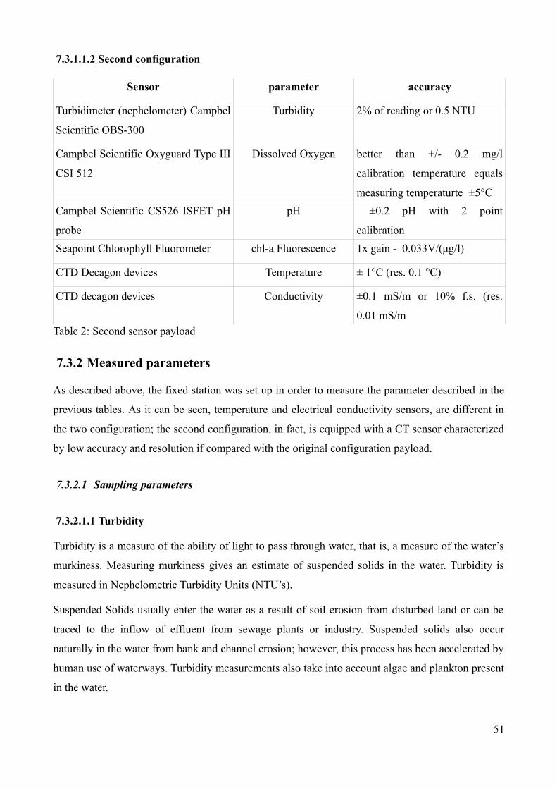
7.3.1.1.2 Second configuration
Sensor parameter accuracy
Turbidimeter (nephelometer) Campbel
Scientific OBS-300
Turbidity 2% of reading or 0.5 NTU
Campbel Scientific Oxyguard Type III
CSI 512
Dissolved Oxygen better than +/- 0.2 mg/l
calibration temperature equals
measuring temperaturte ±5°C
Campbel Scientific CS526 ISFET pH
probe
pH ±0.2 pH with 2 point
calibration
Seapoint Chlorophyll Fluorometer chl-a Fluorescence 1x gain - 0.033V/(μg/l)
CTD Decagon devices Temperature ± 1°C (res. 0.1 °C)
CTD decagon devices Conductivity ±0.1 mS/m or 10% f.s. (res.
0.01 mS/mTable 2: Second sensor payload
7.3.2 Measured parameters
As described above, the fixed station was set up in order to measure the parameter described in the
previous tables. As it can be seen, temperature and electrical conductivity sensors, are different in
the two configuration; the second configuration, in fact, is equipped with a CT sensor characterized
by low accuracy and resolution if compared with the original configuration payload.
7.3.2.1 Sampling parameters
7.3.2.1.1 Turbidity
Turbidity is a measure of the ability of light to pass through water, that is, a measure of the water’s
murkiness. Measuring murkiness gives an estimate of suspended solids in the water. Turbidity is
measured in Nephelometric Turbidity Units (NTU’s).
Suspended Solids usually enter the water as a result of soil erosion from disturbed land or can be
traced to the inflow of effluent from sewage plants or industry. Suspended solids also occur
naturally in the water from bank and channel erosion; however, this process has been accelerated by
human use of waterways. Turbidity measurements also take into account algae and plankton present
in the water.
51

Pollutants such as nutrients and pesticides may bind with suspended solids and settle in bottom
sediments where they may become concentrated. Suspended sediments can also smother aquatic
plants as they settle out in low flows, and clog mouthparts and gills of fish and aquatic
macroinvertebrates.
High turbidity affects submerged plants by preventing sufficient light from reaching them for
photosynthesis. High turbidity also has the capacity to significantly increase water temperature.
Water temperature needs to remain fairly constant so aquatic fauna can survive.
Though high turbidity is often a sign of poor water quality and land management, crystal clear
water does not always guarantee healthy water. Extremely clear water can signify very acidic
conditions or high levels of salinity.
Fig 10: Turbidimeter sensor
the probe uses its optics to emit a near-infrared light into the water. It then measures the light that
bounces back from the water’s suspended particles.
Turbidimeter Campbel Scientific OBS-300
Titanium Body 1500 m Max Depth
Drift <2% per year
Maximum Data Rate 10 Hz
Input Voltage For Voltage Output 5 to 15 Vdc
Input Voltage For Current Output 9 to 15 Vdc
Typical Current Drain For Voltage Output 15 mA
Typical Current Drain For Current Output 45 mA
52

Operating Wavelength 850 nm ±5 nm
Optical Power 2000 μW
Ranges
Turbidity see Turbidity Range Options on page 4
Maximum Concentration*
Mud 5,000 mg/l to 10,000 mg/l
Sand 50,000 mg/l to 100,000 mg/l
Accuracy
Turbidity 2% of reading or 0.5 NTU (whichever is larger)
Concentration
Mud 2% of reading or 1 mg/l (whichever is larger)
Sand 4% of reading or 10 mg/l (whichever is larger)
Table 3: Turbidimeter sensor characteristic
7.3.2.1.2 Oxygen
The amount of oxygen in water, to a degree, shows its overall health. That is, if oxygen levels are
high, one can presume that pollution levels in the water are low. Conversely, if oxygen levels are
low, one can presume there is a high oxygen demand and that the body of water is not of optimal
health.
Apart from indicating pollution levels, oxygen in water is required by aquatic fauna for survival. In
conditions of no or low oxygen availability, fish and other organisms will die.
Oxygen enters water as a result of two processes:
1. Diffusion - diffusion of oxygen into water is accelerated when the water turbulence is increased
and when there is a strong wind blowing. Additionally, oxygen will diffuse into cold water at a
higher rate than it will into warm water.
2. Photosynthesis - during daylight hours, aquatic plants use the sun’s energy to create energy they
can use for growth. A by-product of this process is oxygen which is released into surrounding
water.
53

Ecosystem Type Dissolved oxygen trigger value range
(DO%)
Upland River 60 – 120
Lowland River 60 – 120
Lakes and Reservoirs 90 – 110
Estuaries 60 – 120
Marine 90 - 110
Table 4: Ecosystems oxygen ranges
When the level of Dissolved Oxygen is above or below these ranges, the waterway will
become increasingly stressed.
The Probe
Fig 11: Oxygen sensor
Campbel Scientific Oxyguard Type III CSI 512 Dissolved Oxygen probe
Principle of measurement Membrane covered galvanic oxygen probe
Output signal 2.5 to 5 mV per mg/l
Repeatability better than +/- 0.2 mg/l calibration temperature
equals measuring temperaturte +/-5°CTable 5 Oxygen sensor characteristic
54

7.3.2.1.3 pH
pH is a measure of the acidity or alkalinity of water. It is usually measured by using a colorimetric
test - litmus paper changes colour with increased acidity or alkalinity. pH varies naturally within
streams as a result of photosynthesis. There are a number of reasons that water may have extreme
pH values:
Acidic values
• Geology and soils of the catchment affect pH. Acid soils (these are different from Acid Sulphate
Soils) and rocks such as basalt, granite and sandstone contribute to lower pH in water.
• Acid sulphate soils are a major problem in estuarine areas. These soils form in anaerobic
environments that are rich in sulphur, such as at the bottom of estuaries. If these soils are not
disturbed and are left in anaerobic conditions, they do not pose any threat.
Run-off from bushland areas is slightly acidic.
Alkaline values
• Basic rocks such as limestone contribute to higher pH values.
• Run-off such as fertilisers and detergents cause increased alkalinity.
Extreme values of pH can cause problems for aquatic fauna. For example, fish may develop skin
irritations, ulcers and impaired gill functioning as a result of water that is too acidic. Death of most
aquatic fauna may result from extremely acid or alkaline water.
The pH scale ranges from 0 to 14:
Acidic: 0 to 6.9
Neutral: 7
Alkaline: 7.1 to 14
Table 6: pH ranges
A ph range of 6.5 – 8 is optimal for freshwater. A range of 8 – 9 is optimal for estuarine and
sea water.
The Probe
The submersible CS526 is designed to reliably provide accurate temperature compensated pH
measurements. The pH-sensitive element is SENTRON's Ion Sensitive Field Effect Transistor
(ISFET) semi-conductor, which includes a silver / silver chloride - potassium chloride reference
55

system. This technology is the most significant breakthrough in pH testing in half a century and is
the most powerful pH testing technology available today.
The CS526 is suitable for demanding applications in laboratory and field. The ISFET performs well
in solutions with high solids, moderately aggressive chemicals, and biological materials. Clogging
and junction contaminating conditions are well tolerated.
Fig 12: pH sensor
Campbel Scientific CS526 ISFET pH probe
Range 1 to 14 pH
Accuracy ±0.2 pH with 2 point calibration
24 hr drift < 0.15 pH (after 15 min soak in pH 7 at 25°C)
Operating
Temperature 10° to 40°C
Water Pressure 0 to 700 kPa (0 to 101.5 psi)
Storage Temperature 20° to 30°C
Power Requirement
Source 5 Vdc
Load 15 mA maximum
Output TTL logic, 2400 bps 8 data bits, no parity, 1 stop
bit
Table 7: pH sensor characteristic
56

7.3.2.1.4 Fluorescence
In aquatic environments, the measurement of chlorophyll a is used as an indicator of autotrophic
biomass as the pigment is essential for the process of photosynthesis for all autotrophic organisms.
Chlorophyll a is the 1-2% of the dry weight of the organic matter of the algae. From the
measurement of the chlorophyll is thus possible to deduce the content of organic substance using
the conversion factors. The ratio between organic carbon and chlorophyll varies between species,
depending on the different environmental and physiological conditions. The laboratory analysis for
the quantification of chlorophyll are generally performed by means spectrophotometric and
fluorimetric techniques. The spectrophotometric and fluorimetric methods are widely used for field
surveys. The fluorimetric technique, up to 50 times more sensitive than spectrophotometric, allows
the use of small volumes of sample and promote the in-vivo measurement of chlorophyll-a.
Fig: 13: Fluorescence sensor
Seapoint Chlorophyll Fluorometer
Power Requirements 8-20 VDC, 15mA avg, 27mA pk
Output 0-5.0 VDC
Output Time Constant 0.1 sec
Power-up Transient 0.6 sec
RMS Noise (typ.)
57

30x gain 3 mV
10x gain 1 mV
3x gain <1 mV
1x gain <1 mV
Excitation Wavelength 470 nm peak, 30 nm FBHM
Emission Wavelength 685 nm peak, 30 nm FBHM
Sensing Volume 340 mm3
Sensitivity/Range
30x gain 1.0 V/(μg/l) 5 μg/l
10x gain 0.33 V/(μg/l) 15 μg/l
3x gain 0.1 V/(μg/l) 50 μg/l
1x gain 0.033V/(μg/l) 150μg/l
Table 8: Fluorescence sensor characteristic
7.3.2.1.5 Electrical conductivity
Conductivity is a measure of the ability of water to pass an electrical current. Conductivity in water
is affected by the presence of inorganic dissolved solids such as chloride, nitrate, sulphate, and
phosphate anions (ions that carry a negative charge) or sodium, magnesium, calcium, iron, and
aluminium cations (ions that carry a positive charge). Organic compounds like oil, phenol, alcohol,
and sugar do not conduct electrical current very well and therefore have a low conductivity when in
water. Conductivity is also affected by temperature: the warmer the water, the higher the
conductivity. For this reason, conductivity often is reported as conductivity at 25 degrees Celsius
(25 C).
The probe used to measure conductivity was originally an amperometric system which had two
electrodes spaced one centimeter apart from each other.
The amperometric method applies a known potential (voltage, V) to a pair of electrodes and
measures the current (I). According to Ohm's law: I=V/R where R is the resistance. The higher the
current so obtained, the greater the conductivity. The resistance in this method unfortunately is not
constant even though the distance may be fixed. Salt deposition on the electrodes due to
electrolysis can vary the resistance. For low to medium levels of conductivity (< 2 mS/cm) this
58

may be sufficient, but for greater accuracy and for higher levels, a different method is required.
A potentiometric method is based on induction and eliminates the effects of polarization common to
the amperometric method. The potentiometric method employs four rings: the outer two rings
apply an alternating voltage and induce a current loop in the solution while the inner rings measure
the voltage drop induced by the current loop. This measurement is directly dependent upon the
conductivity of the solution. A shield around the rings maintains a constant field by fixing the
volume of solution around the rings.
Because a potentiometric (4-ring) conductivity sensor is not limited by electrolysis which
commonly affects amperometric probes, it can be used to measure a much wider range of
conductivities. Practically, stainless steel rings can be used. But, the preferred metal is platinum
because it can withstand higher temperatures and produces a more stable reading. Platinum sensors
are also easier to clean. Advanced microprocessor conductivity instruments can vary the voltage
applied to the sensor which enables them to extend the range of a potentiometric probe even further.
This technique allows advanced meters to be able to measure both high and low conductivities as
well as the ultra low conductivity of deionized water with one probe.
Another method of conductivity measurement uses an inductive probe (sometimes referred to as a
toroidal sensor). Typically these are found in industrial process control systems. The sensor looks
like a donut (toroid) on a stick. The advantage of this technology is measurement without any
electrical contact between the electrode and the process fluid. The probe uses two toroidal
transformers which are inductively coupled side by side and encased in a plastic sheath. The
controller supplies a high frequency reference voltage to the first toroid or drive coil which
generates a strong magnetic field. As the liquid containing conductive ions passes thrugh the hole
of the sensor, it acts as a one turn secondary winding. The passage of this fluid then induces a
current proportional to the voltage induced by the magnetic field. The conductance of the one turn
winding is measured according to Ohm's law. The conductance is proportional to the specific
conductivity of the fluid and a constant factor determined by the geometry and installation of the
sensor. The second toroid or receiving coil also is affected by the passage of the fluid in a similar
fashion. The liquid passing through the second toroid also acts as a liquid turn or primary winding
in the second toroidal transformer. The current generated by the fluid creates a magnetic field in the
second toroid. The induced current from the receiving coil is measured as an output to the
instrument. The controller converts the signal from the sensor to specific conductivity of the
process liquid. As long as the sensor has a clearance of at least 3 cm the proximity of pipe or
container walls will have a negligible effect on the induced current.
59

7.3.2.1.6 Temperature
Temperature along with other factors such as salinity is very important in determining the
movements of the masses of sea water, which in turn have a direct impact on the processes of water
oxygenation and circulation of nutrients.
Temperature measurement is significant because it affects the amount of dissolved oxygen in the
water. The amount of oxygen that will dissolve in water increases as temperature decreases. Fresh
water at O °C will hold up to 14.6 mg of oxygen per litre, while at 30 °C it will hold only up to 7.6
mg/L.
Temperature also affects the rate of photosynthesis of plants, the metabolic rate of aquatic animals,
rates of development, timing and success of reproduction, mobility, migration patterns and the
sensitivity of organisms to toxins, parasites and disease. Life cycles of aquatic organisms are often
related to changes in temperature. Temperature ranges for plants and animals can be affected by
man made structures such as dams and weirs and releases of water from them.
The Probe
7.3.2.1.7 Temperature and Electrical conductivity second configuration
Decagon Devices Temperature Conductivity and Depth sensor
Temperature
Accuracy ±1°C
Resolution 0.1°C
Range -40°C to +50°C
Bulk Electrical Conductivity
Accuracy ±0.01 dS/m or ±10% (whichever is greater)
Resolution 0.001 dS/m
Range 0 to 120 dS/m (bulk)
General
Dimensions 9 cm (1) x 3.4 cm (w)
60

Measurement Time 300 ms (milliseconds)
Power Requirements
Input 3.6 - 15 VDC, 0.03 mA quiescent,
Input 10 mA during 300 ms measurement
Output Serial (TTL), 3.6 voltage levels or SDI-12
Operating Temperature -40 to 50 °C
Table 9: CTD sensor characteristic
7.3.2.1.8 Salinity (derived variable from T and C)
The salinity expresses the quantity in grams of salts contained in one kilogram of sea water . The
measure is commonly expressed through the Practical Salinity Scale PSS (Fofonoff & Millard,
1983) an a-dimensional unit (PSU) obtained as a function of Temperature and Conductivity
The Practical Salinity Scale of 1978 is the official definition:
S = 0.0080 - 0.1692 K151/2 + 25.3851 K15 + 14.0941 K153/2 -7.0261 K152 + 2.7081 K155/2
K15 = C (S,15,0) / C (KCl,15,0)
2 ≤ S ≤ 42
where C (S, 15, 0) is the conductivity of the sea-water sample at a temperature of 15°C and standard
atmospheric pressure, and C (KCl, t, 0) is the conductivity of the standard potassium chloride (KCl)
solution at a temperature of 15°C and standard atmospheric pressure. The standard KCl solution
contains a mass of 32.435 6 grams of KCl in a mass of 1.000 000kg of solution.
The Mediterranean has values ranging from 37 in the west , to 39 in the east. The most widely used
method for measuring the salinity , however, is based on the electrical conductivity . Salinity is a
very important factor in the life of marine organisms and their distribution , as every body can
tolerate variations in this parameter only within certain limits. It follows that any form of pollution
that alters this parameter will produce changes in the composition of flora and fauna of the area
concerned . Measuring salinity is very important, in fact through its measurement can be
highlighted discharges of fresh water due to the stratification that will be created between the water
masses having different densities .
61

8 Methods
Real time data, or near real time data related to fixed observing stations, play a fundamental role
within important thematics like model data assimilation for forecast and climatology. For this
reason, data quality assurance and quality control procedures are required (Manzella & Gambetta,
2013).
In particular, quality assurance is based on seven steps as described in the Quality Assurance of
Real Time Oceanographic Data, QUARTOD project (Babin et al., 2009). Even if quality control for
such data involves a small number of qc working procedures compared with the final 'archived
data', nonetheless, the following steps should be performed:
1) Every real-time or near real-time observation distributed to the ocean community must be
accompanied by a quality descriptor (qc number).
2) All observations should be subject to some level of automated quality test.
3) Quality flags and quality test descriptions must be sufficiently described in the accompanying
metadata.
4) Observers should independently (verify or calibrate a sensor before deployment).
5) Observers should describe their methodology/ calibration within metadata.
6) Observers should quantify the level of calibration accuracy and associated expected error bounds.
7) Manual checks on the automated procedures, the real-time data collected, and the status of the
observing system must be provided by the observer on a time-scale appropriate to ensure the
integrity of the observing system.
For the above reasons, one of the most important issue of this project was to find a standard
procedure to calibrate raw data coming from the daily downloads, in order to produce a verified and
validated dataset for the 'near real time' mode.
In the following chapters it will be discussed the parameter calibration procedures and the problem
related to obtain the near real time data assurance. Also the Quality control software, and the
Seadatanet standardization tools utilized for the final quality controlled archiving dataset will be
described.
62

8.1 Calibration procedures
8.1.1 Turbidity
Turbidity sensor is an Optical Back scatter nephelometer. Standard Laboratory calibration is
performed against formazin (EPA, 1993). Because of the impossibility to perform such calibration
in our laboratory, it was decided to perform the calibration utilizing field samples of total suspended
matter.
Water samples were collected during the maintenance activities by means a NISKYN bottle.
Laboratory analysis were conducted to detect the total suspended matter concentration as described
in APAT CNR IRSA, 2003.
The following graph represents the logarithmic regression obtained for turbidity data of the probe
against suspended solid data obtained through laboratory determination conducted on field samples.
Fig 14: Turbidity calibration. The figure shows the experimental logarithmic regression between sensor NTU and Suspended solid
from field samples
63

The following logarithmic equation:
Y = 3.625774312 * ln(X) + 5.533343666
r2 = 0.911413
was utilized to convert NTU to suspended matter (mg/l)
8.1.2 Oxygen
Oxygen calibration were performed utilizing the standard procedure reported in the sensor operator
manual.
O2_air_mg = 10.29 as from fresh water oxygen solubility table for salinity 0 psu and t = 14,00 °C;
O2_sat_air_mv = 41.2 millivolt output corresponding to O2_air_mg;
M_corr = O2_air_mg /O2_sat_air_mv; coefficient for millivolt to ppm conversion
O2mv = millivolt Output measurement.
O2ppm = M_corr * O2mv;
8.1.3 pH
The calibration of the pH sensor was performed plotting the pH values of the Idronaut reference
probe against the mV output of the ph sensor.
The following relation derive fro a linear regression
pHcal = 0.00285*pHmv + 6.152
64

8.1.4 CHL-a
Calibration of fluorometer data were performed against monthly field samples .
After the laboratory analysis for the chl-a spettrophotometric determination, a linear regression
output was obtained
Laboratory analysis of chlorophyll-a were performed according to standard methods (Lazzara et al.,
1990, Jeffrey & Humphrey, 1975).
Fig 15: Fluorescence calibration. Fluorescence unit plotted against chl-a field samples data
The above graph shows the linear regression between fluorescence data and chl-a data with the
following equation:
Y = 0.4802167069 * X + 0.2902080327
r2 = 0.896956
65

Thos relation was implemented into the Matlab routine in order to convert fluorescence data to
biomas expressed by mg/l of chlorophyll-a.
Even if the coefficient of determination of the regression seems not to be excellent, it is reasonable
satisfactory considering the hard sampling conditions (low maintenance- high fouling) in which the
fluorometer works.
8.1.5 Electrical conductivity
Electrical conductivity was calibrated against a reference CTD probe IDRONAUT OCEAN
SEVEN 316.
First configuration calibration, gave excellent regression output, but the second configuration
calibration, due to low accuracy of the T sensor and Conductance cell, was hard to perform.
Acquired data presented spikes and a value of Standard Deviation of 1.0527719.
Fig 16: The figure shows three days conductivity data acquisition: Reference probe Idronaut (blue line; Fixed station probe red line.
Furthermore the sensor design did not full comply the seawater conductivity sensor capabilities. For
example the temperature compensations internal algorithm. So that, it was possible understand the
internal temperature compensation algorithm. Such algorithm was reported in the Hand book 60 of
US laboratory of salinity and it is suitable for determination of conductivity and salinity of ground
water. For this reason, the compensation did not work properly for typical seawater conductivity
values.
So that, it was possible de-compensate all the data in order to obtain not temperature compensate
conductivity raw data.
66

A Matlab routine was written in order to perform such task. appendix A.
After that, in order to obtain a more accurate conductivity data, a new temperature compensation
procedure was performed. The conductivity sensor was tested with seawater at constant salinity
value of 37.7 for different temperatures.
The following equation of temperature effect on conductivity measurement was found:
Y = 11.84772573 * ln(X) + 9.182759992
r2 = 0.871451
Fig 17: temperature compensation curve performed at 37.7 psu
67
Conductivity was compensated at 20°C degrees as follow:
Cond20 = Cond measured - K
K = a * (ln(20) - ln(t))
a = 11.84772573
Cond measured = de-compensed conductivity value
t = measuring temperature.
In the following graph are represented the re-compensated value of the probe and reference
conductivity values. In this case data are less variable with a value of the standard deviation of
0.9457.
Fig 18: The figure shows three days conductivity data acquisition : Reference probe Idronaut (blue line); Fixed station probe re-
compensed@20°C (red line).
Conductivity data value compensated by means this new equation, were fitted with weighted
average in order to eliminate the spikes.
68

Fig 19: weighted average data
Data were than utilized to perform the inter-calibration against the conductivity data of the
reference probe.
Fig 20: Intercalibration between reference conductivity data and new re compensated fixed station data
69

The above graph represent the conductivity data of the probe against the reference data. The linear
regressions:
Y = 0.2346884644 * X + 39.10423852
r2 = 0.274738
as it is shown by the coefficient of determination, the calibration of the conductivity sensor do not
give reliable results.
8.1.6 Temperature
Temperature data were calibrated against a reference CTD probe IDRONAUT OCEAN SEVEN
316.
Even thought the temperature sensor of the second configuration system presented the same
problem as the conductivity sensor, due to its low accuracy, nonetheless the inter-calibration with
the reference CTD gave good regression outputs as shown in the figure.
Fig 21: three days temperature data acquisition. The blue line represents the reference probe data, while the red line represents the
fixed station temperature data
70

Fig 22- The figure shows the linear regression between the reference temperature from Idronaut and the temperature sensor of the
fixed station probe.
The equation of the linear regression is:
Y = 0.9625070318*X + 0.5563518493
r2 = 0.932676
71

8.1.7 Salinity
Salinity calibrated data were obtained by means the application of the UNESCO International
Equation of State (IES 80) as described in Fofonoff and Millard 1983, utilizing the T and C
calibrated values.
As the conductivity sensor was impossible to calibrate with a reasonable r2, salinity was calculate
from conductivity raw data. Bad values were checked with the QC processes described in the next
paragraph, and set to “NaN” in the output dataset.
In the following figure are represented the salinity trend along three days of acquisition.
Fig 23- in the figure are represented the three different trend of salinity data obtained by the CT calibration procedures compared
with the salinity obtained by the reference probe Idronaut.
As it can be seen in the graph, the we have plotted the salinity values along the time related to four
different calculations:
1) The blue line represent the reference salinity from the probe Idronaut;
2) the red line represents salinity calculated from the temperature and conductivity calibrated
values by means the equations obtained from the regressions;
3) the green line represents salinity calculated from calibrated temperature and non calibrated
conductivity;
the purple line represents salinity calculated from non calibrated temperature and non calibrated
conductivity.
The graph highlights that the “calibrated salinity” (red line in the graph) is the best approximation
for the reference salinity.
72

9 Near real time data control: Quality Assurance and quality Control software
9.1 The acquisition system operations
The electronic device, the CR1000 Campbel scientific data logger, is responsible for turning on the
the sensors. The data logger tasks are set into an internal program, compiled with all the instructions
indispensable to manage the sensors start and stop procedures, the data acquisitions, the data
transformations and the data pre-elaboration output.
a) The electronic devices is programmed to sample seawater parameters to provide one raw data
each 20 minutes plus the standard deviation. In the present configuration, each data derives from the
median of 30 raw data collected for 30 seconds (1 data/sec).
b) Digital data are transformed from the sensor output into physical values, while analogical data
are converted into parameters unit during the post processing procedures (Matlab routines). Data are
stored into the cr1000 internal memory and deliver twice a day to OLINDA FTP server: at 8:00:00
and 16:00:00 hours.
c) The transformation and the calibration of data values, are performed by means Matlab, through
an ad hoc routine.
9.1.1 Data download
Fig 24- Online Olinda Portal to data download
73

From the olinda web page, data are daily downloaded to perform data conversion and data
calibration in order to provide an input data set for the QC (Quality Control procedures) and for the
data format standardization.
9.1.2 Data file name
Download command, generates a data file in which data span from the 00:00:00 daytime of the start
pre-set day to the last data available of the end pre-set day.
The situation displayed in the above figure, for example, will generate a data file spanning from
00:00:00 of gen-10-2014 to 08:00:00 of feb-10-2014 if we are downloading the file between 8:00
an 16:00.
File name will be: Dati-8702_1-2014110-2014210
and the file type will be an Excel file.
As normal procedures take into account daily downloads data files will be referred to a time interval
between the 00:00:00 of a day and the 08:00:00 of the day after.
9.1.3 Matlab pre-formatting task
Daily datasets are manually checked for data anomalies and corrected. “0” values in the data fields
are changed into “NaN” string; while the lack of dates is reconstructed in order to fill the time gap,
setting the associate data at “NaN”. Furthermore, in order to avoid dates overlapping, the firsts
seven hours are deleted.
Such modified file, is saved to a csv file, accepted by the Matlab routine.
74

Fig 25- Flow chart of the download procedures and the data process.
The csv file name is always referred to the date of the last data within the downloaded file.
9.1.4 The Matlab routine
The first Matlab routine called ST_Prox.m, extracts data variables from the original raw data matrix
in order to perform the following tasks:
1) transformation of raw data value (sensor output) to parameters unit (Fluorescence unit into
chlorophyll unit);
2) calibration of data values by means calibration relations and coefficients;
3) preliminary graphical outputs;
4) save calibrated data to a new output file.
75
Dati-8702_1-yyyymmgg-yyyymmgg.xls
OLINDA DOWNLOAD
Anomalies corrections
ST_Prossimita_Civ_yyyymmgg.csv
ST_Prossimita_Civ_yyyy_mmgg.csv
Matlab routines

following figures show some preliminary Matlab graphs.
Fig 26- Preliminary matlab graphical output of the calibrated parameters
76

9.1.5 Data Quality Control
Fig 27- Flow chart of the data acquisition steps: from the data download through the quality control procedures till the final outputs
77
The above figure illustrates the flow chart of the QC procedures.
The QC procedures, actually starts from the preliminary Matlab data outputs.
By means an ad hoc Matlab routine, “varsmooth”, data can be smoothed and then the output data
matrix is formatted in order to comply the QCDAMAR quality control software format
requirements.
9.1.5.1 QCDAMAR the Spanish Oceanographic Quality Control software
Software developed at IEO consists of three main and closely related three components dealing with
data analysis, database storing and web access.
Since 1994 the Marine Department of the Spanish Oceanographic Institute develops system for
archiving and quality control of oceanographic data. The work started in the frame of the European
Marine Science & Technology Programme (MAST) when a consortium of several Mediterranean
Data Centres began to work on the MEDATLAS project.
A complete description of main procedures used in the present software can be found in the
following references: “MEDATLAS GROUP 1994”, “MEDAR-MEDATLAS PROTOCOLS 1999”,
“UNESCO 1993” y “REINIGER R.F. and ROSS C.K., 1968”. This section contains only a brief
summary of the Medatlas format and the quality controls as proceeded in the QCDAMAR software.
Here is the list of quality control procedures implemented in the program for vertical profile
acquisitions and for time series acquisitions:
check for duplicates
- duplicate cruises
- duplicate profiles
- manual validation : ( keep only one)
check stations date and the position
- check the date
- check the ship velocity: (< 15 knots)
- check the sounding: ( reference ETOPO5, interpolated from the 9 nearest points)
78

- check the location: (visualization)
- check global header profile: ( time position and depth)
-manual validation: ( Edit file and change flags)
check data points
- check for acceptable data: PRES must be present
- check for impossible regional values: value must be between the range given in the files
v_total.dat and v_region.dat for each parameter and each zone.
- check for increasing depth:
- check for pressure: reference profile sounding or ETOPO5 bathymetry.
values<sounding 5% or between 0.5 or 2 when using reference statistics.
- check for temperature and salinity : reference profiles MEDATLAS climatology. (*)
value must be between the data reference ± a range.
data reference = values interpolated from the nearest reference profile at the measured
pressure level.
acceptable range of variation = 5, 4 or 3 times of the interpolated standard deviation of
reference at the same level.
(*) if you want to use another climatology ( i.e. , Brasseur P) or bathymetry the format of the split
files must be preserved.
- check for constant profiles: check constant values for each parameter.
global parameter quality flag = 4.
- check each pressure: comparing with the bottom or the ETOPO5 reference
- check for spikes: the algorithms used to detect the spike are:
for the top and bottom pressures: (v2-v1)/(p2-p1)>pic_borne
for the other pressures depends on the type of data: bottles or CTD.
- check for density inversion: the algorithm used is (dens(n)-dens(n-1) ≤ EPS (*)
where dens(n) is the potential density anomaly at level n computed from equations of the state
79

of sea water. ( ref: FOFONOFF and MILLARD,1983 and MILLERO and POISSON, 1981). (*)
The noise value EPS is taken from the file “v_total.dat”.
- global quality check for a profile: one quality flags per parameter in the header profile
each flag value is computed from the corresponding parameter flags at each level.
- check parameter distributions and flags: visualization in colour for the flags.
- manual validation: changing the flags and writing the DM history by editing the file.
Time series header control:
Additionally to the quality control procedures for headers mentioned above, in case of time series
some new checks were introduced:
- Control of start date:
start date and time (year, month, hour, minute and seconds) in the header has to be the same or
earlier than the date and time of the first (start) data record.
- Control of end date:
end date and time in the header has to be the same or later than the date and time of the last (end)
data record. In case of lacking of the end date in the header, last date of end record is written instead
and the correspondent quality flag is changed to 5.
- Control of end position:
if the distance between start and end positions > 1 nautical mile the flag is changed to 4; in case of
no value of final position, it’s changed to the start position value and its correspondent flag takes
value 5.
For cases of movement, i.e. when latitude and logitude are present as parameters of a time serie, end
position in the header is compared to the end time serie record position.
- Control of “SENSOR DEPTH”:
if its value is greater than DEPTH the flag = 4.
- Control of “DISTANCE TO THE BOTTOM”:
if the sum of “SENSOR DEPTH” + “DISTANCE TO THE BOTTOM” differs greatly
80

from“DEPTH” the flag = 4.
- Control of duration:
if the duration in the header is less than that calculated from data records, the flag = 4. If the
duration value in the header is absent, real calculated duartion is written down instead and the flag
is changed to 5. Deafault value = -9.
Time series data control:
Apart of general headers control for valid date, time, etc., identical to water observations, some
additional tests are performed in case of time series:
·beginning date in the header must be prior or equal to the date of the first measured data value
- end date must be greater than the beginning date, as well as it can't prior to the last measured data
value. If end date is absent, the date of last measured data is assigned to the end date and the flag is
changed to "5".
- duration in days given in the header is compared to its real value calculated from observations
- sensor depth in the header is compared with measured data pressures (PRES) or depths below sea
surface (DEPH). Maximum allowed difference is read from editable text file "v_sensor.dat"
- value of the sum of sensor depth and distance to bottom minus 10% of this sum can't be greater
than depth
- the values of maximum, minimum and delta, necessary for impossible regional values test of time
series, are contained now in the file "v_series.dat"
- checking for descending time order is performed
- time continuity check is applied to each data measurement. Time shift between data values is
compared with sampling rate
If optional test for “bottom sounding” is checked, test is performed by comparing the bottom
sounding value with -+20% of max and min values of ETOPO depths chosen from 9 nearest
ETOPO points.
If optional test for “pressure statistics” is checked, test for pressure is performed during full QC.
Pressure values at all levels are compared with sounding (if recorded) or with statistical depth value
81

from ETOPO.
Detailed description of testing procedures implemented in QCflag can be found in Medar-Medatlas
Project Protocol.
The output files with the same names and QC extension are found in the same directory. The files
with the list of errors (if there any) have the ERR extension and the same names as the input files.
The ETOPO5 data are interpolated and should be used for primary rough control of sounding.
The files "v_region.dat", v_total.dat" and "v_noise.dat" contain limit control values for water
observations, while in the files "v_series.dat" and "v_sensor.dat" there are limit check values for the
case of time series.
The hydrological regime of a particular area of study can be characterized by a great variability. To
enhance the performance of quality control of impossible regional values for this area the user can
introduce in the file ‘v_region.dat’ individual limits for parameters for that area.
Quality flag procedures
The flags indicating data quality are those currently used in the GTSPP real time quality control and
recommended in the MAST/IOC Manual (p310):
0 = no QC performed on the element (NULL is equivalent to 0 )
1 = QC performed; element correct
2 = QC performed; element inconsistent with statistics but no obvious anomaly)
3 = QC performed; element doubtful (= questionable)
4 = QC performed; element bad (= erroneous = wrong)
5 = the value was changed (=interpolated) after QC
6 -8 = reserved
9 = missing value
Each numerical value must have a quality flag.
- Date and time control: all time series records must be consecutive in time, i.e. each next record
must have date and time equal to that of previous record plus time interval of the serie data. On the
contrary the flag for all parameters of erroneous record is put to 4 and further analysis is stopped.
82

- Pressure/Depth parameter control: if absolute value of the difference between pressure/depth in
each record and “SENSOR DEPTH” is greater than a value established by the user, the flag is
changed to 3.
- Broad range: if parameter values don’t enter in the established diapason, correspondent flag is = 4.
- Delta check: if absolute value of the difference between consecutive data records of any parameter
is greater than limit established for that difference, the flag = 3.
- Position parameters check: if velocity calculated between consecutive records when latitude and
longitude parameters are present (case of movement) is greater than established maximum ship
velocity (20 knots), the flag is set to 3.
Fig 28- QCDAMAR QC procedures flow chart
In the following figures are represented the input file and the output QC file.
As it can be seen, each Meta-data and single data are flagged with the appropriate QC number.
83
ST_Prossimita_Civ_yyyymmgg_QC.csv
QCDAMAR INPUT FILE
Parameter range setting
QC perform

Fig. 29- Matlab output: data are transformed into physical values and calibrated against field samples
Fig: 30 Matlab output: Data and meta-data are formatted to comply QCDAMAR input requirements
84

Fig: 31 QCDAMAR output: Data and meta-data are flagged QC value
85
Metadata
Flagged data

9.1.6 Seadatanet data and meta-data Standardization procedures
The above procedure, allows to perform a quality control on the data set, flagging each data, with
its appropriate quality value, following the international qc scale (see before), adopted by MEDAR-
MEDATLAS
QCDAMAR software generates a MEDATLAS file format, so it is necessary to convert it to an
ODV (Ocean data View) file format, as it represent the European standard for data and Meta-data
To perform such task it is help full the use of SDN software’s, NEMO and MIKADO.
NEMO allows the conversion from a generic data file format (e.g. ASCII) to ODV data file format,
also performing the variable codes matching (user-seadatanet) through the adoption of common
vocabularies.
Here is represented an example of common vocabulary utilized to match chl-a parameter.
SDN code Code term Code abbr Code def
CPWC Chlorophyll
pigment
concentrations in
the water column
WC_ChlPigs Includes all variants of chlorophyll expressed
in terms of per unit volume or unit area of the
water column. Does not include data
expressed per unit mass of SPM.
Tab.9- P02 SDN vocabulary for chlorophyll pigment description
The following table gives the list of the principal common vocabularies.
Library Title
C16 SeaDataNet sea areas
C17 ICES Platform Codes
C19 SeaVoX salt and fresh water body gazetteer
C32 International Standards Organisation countries
C34 Activity purpose categories
C35 European Nature Information System Level 3 Habitats
C36 Monitoring activity legislative drivers
C37 Ten-degree Marsden Squares
86

C38 SeaDataNet Ports Gazetteer
C45 Marine Strategy Framework Directive descriptors
C46 Marine Strategy Framework Directive criteria
C47 Marine Strategy Framework Directive indicators
C64 United Kingdom Charting Progress 2 sea regions
C77 SeaDataNet Cruise Summary Report data categories
C86 SeaDataNet contact and security access roles
C97 NERC Vocabulary Server Version 1 mappings index
GS3 Geo-Seas adjusted Folk sediment lithology classes
GS4 Geo-Seas geological sample colours
GS5 Geo-Seas sediment grain-size skewness descriptors
GS6 Geo-Seas sediment grain-size kurtosos descriptors
GS8 Geo-Seas Seismic Methods
GS9 Geo-Seas Seismic Survey Dimensionality
GSA Geo-Seas Seismic Data Product Types
GSB Geo-Seas Seismic Receiver Types
GSC MGD77 Bathymetry Sound Velocity Correction Codes
L02 SeaDataNet Geospatial Feature Types
L03 SeaDataNet Measurement Periodicity Categories
L05 SeaDataNet device categories
L06 SeaVoX Platform Categories
L07 SeaDataNet data access mechanisms
L08 SeaDataNet Data Access Restriction Policies
L10 SeaDataNet geographic co-ordinate reference frames
L11 SeaDataNet depth measurement reference planes
L12 SeaDataNet parameter quality control procedures
87
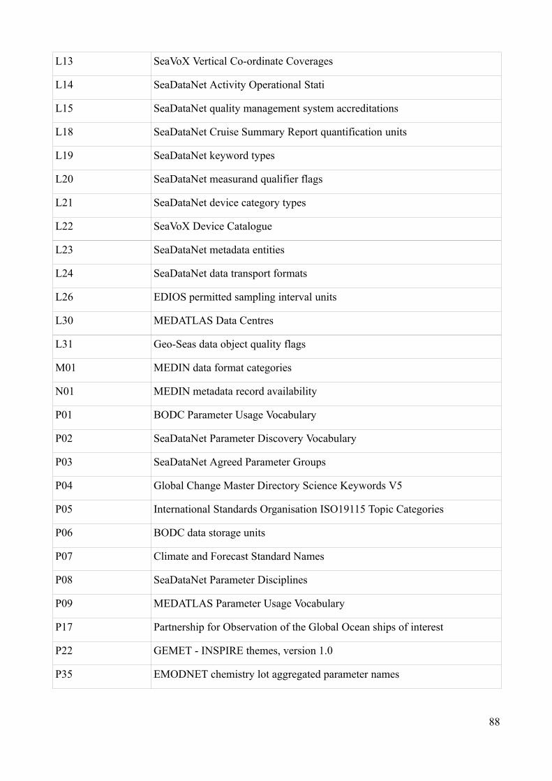
L13 SeaVoX Vertical Co-ordinate Coverages
L14 SeaDataNet Activity Operational Stati
L15 SeaDataNet quality management system accreditations
L18 SeaDataNet Cruise Summary Report quantification units
L19 SeaDataNet keyword types
L20 SeaDataNet measurand qualifier flags
L21 SeaDataNet device category types
L22 SeaVoX Device Catalogue
L23 SeaDataNet metadata entities
L24 SeaDataNet data transport formats
L26 EDIOS permitted sampling interval units
L30 MEDATLAS Data Centres
L31 Geo-Seas data object quality flags
M01 MEDIN data format categories
N01 MEDIN metadata record availability
P01 BODC Parameter Usage Vocabulary
P02 SeaDataNet Parameter Discovery Vocabulary
P03 SeaDataNet Agreed Parameter Groups
P04 Global Change Master Directory Science Keywords V5
P05 International Standards Organisation ISO19115 Topic Categories
P06 BODC data storage units
P07 Climate and Forecast Standard Names
P08 SeaDataNet Parameter Disciplines
P09 MEDATLAS Parameter Usage Vocabulary
P17 Partnership for Observation of the Global Ocean ships of interest
P22 GEMET - INSPIRE themes, version 1.0
P35 EMODNET chemistry lot aggregated parameter names
88

P64 Global Change Master Directory Science Keywords V6
S11 BODC parameter semantic model biological entity development stage terms
S25 BODC parameter semantic model biological entity names
V12 SeaDataNet Vocabularies
Tab 10- Adopted common vocabularies list
NEMO conversion procedures take into account all the informations inside in the data file; from
meta-data, to data values and if any, the data qc flags.
Within the conversion procedures, user is asked to choice the appropriate parameter code by means
the utilization of the common vocabulary.
The conversion process, also adds to the output file some fundamental information about the data
originator an distributor.
The following screen shots show the NEMO conversion steps to ODV file data format.
89

90

Fig.32 - ODV data file format with SDN semantic lines for parameters code matching
The last figure represents the screen-shot of the ODV data file format obtained by means the
NEMO software.
As can be seen, the first lines of the file represent the seadatanet semantic lines utilized by ODV
software and the Seadatanet infrastructure to perform the match between the users parameters and
the international parameters codes according to the Seadatanet common vocabularies.
Fundamental informations, like date, time and geographical references, are located within the data
header.
ODV software is able to open such files loading all meta-data and data at the same time.
ODV visualizations allow to perform a visual quality data control to check the reliability of the
automatic quality control procedures performed by means QCDAMAR. Furthermore the possibility
to manage quality flags represent a fundamental tool to refine and adjust the overall quality of the
dataset.
Such visual quality control is a fundamental step of the entire Qc process (UNESCO-IOC, 2010)
allowing in some case to highlight data anomalies otherwise impossible to check.
In the following figures it is represented two ODV visualizations.
The first figure represents the entire dataset, in which it is possible to see the spikes related with the
91
SDN semantic lines

values = 0 of salinity.
Fig. 33- total raw data not filtered for “good values”
As the QC procedures flag these values with “qc=4” (bad value), ODV “sample selection criteria”
tool allows not to show them plotting just the good values (qc=1).
The second figure depicts the “good value output”.
Fig. 33- total calibrated data filtered for “good values”
92

10 ResultsThe procedures illustrated above (downloads and QCDAMAR quality control), were performed
every day onto daily downloads, in order to obtain a daily dataset with data checked for good
quality. Such dataset was upload daily on to an FTP server and are shared in the on-line portal of the
Port Authority of Civitavecchia.
At the same time, each fifteen days, data were collected together to provide the SEADATANET
EDIOS series for the final archiving procedure of the data and the meta data into the standard
format accepted by SEADATANET infrastructure.
10.1 Adopted output data format for finally archiving and sharing
MIKADO is the Seadatanet software dedicated to the standardization of metadata following the ISO
19115 and 19134 ISO standard.
Makado softeare was utilized linked to Nemo conversion software to generate the XML file related
to the EDIOS (European Directory of Initial observing Systems:
EDIOS program
EDIOS PLATFORM
93

EDIOS SERIES
Presently forty edios series related to fifteen consecutive days acquisitions are archived into local
server. Related dataset are described by the CDI XML file
10.2 Data type description and Seadatanet parameters code
As described above, the project parameters measured by the fixed station are:
Suspended Matter, Dissolved Oxygen, pH, Phytoplankton biomass, Conductivity, Temperature and
Salinity (from Temperature and conductivity).
As the sensors installed on the measuring platform, provide data with its own outputs, it was
necessary to transform data into physical variables (see chapter 7) and then to calibrate the sensors
output against reference probes, or against field samples. According to it was possible to define the
94

final parameters output as follow described:
Sensor output m.u. Calibration
method
Parameter
output
m.u. SDN CODE
NTU nephelometric
unit
field samples Total
Suspended
Matter
mg/l TSED
O2 mv Field/reference
/Factory
Dissolved
Oxygen
ml/l DOXY
pH mv Reference
sensor
pH pH unit ALKY
Fluorescence rel. U. field samples CHL-a mg/m3 CPWC
Electrical
conductivity
mS/cm Reference
sensor
Electrical
conductivity
S/m CNDC
Temperature °C Reference
sensor
Temperature °C TEMP
Salinity – Reference
sensor
Salinity PSU PSAL
Table 11- Sensors output conversion to SDN parameters code
95

11 Discussions
In the following figures are represented the total amount of data deriving from the quality control
procedures and the standardization of the entire data set by means the application of the common
vocabulary parameter names, and the qc seadatanet international qc scale.
The data set span from the July 2011 to November 2014. As described above, for each months a 15
days time series had been created and archived into the standard data and metadata format by
means SEDATANET software and tools.
As shown in figure below, the raw data can describe the overall trend of the parameter, but it is
possible to see at the same time the maintenance event, that appear along the graphs as “0” values.
Actually these values correspond to event of “in air acquisition” during the cleaning activities.
Fig 34- original raw data transformed to physical values, without QC procedures: note the noisy parameters signals and the spikes.
Furthermore it is clear the presence of a lot of noise and spikes related to anomalies in the data
acquisition due to both environmental and sensors particular events.
96

Fig 35- Original raw data were checked for bad value and then transformed and calibrated. The ODV plots related just to the “good
values” data show less variability respect to the original data.
Quality control procedures, allow to individuate these bad events, in a near automatic mode,
flagging with qc = 4 all the samples that lye outside the parameters accepted range set in the QC
software. At the same time a further visual quality control can be perform to set the proper flag to
those data not detected as “bad” or “doubtful” by means the automatic procedures. This is the case,
for example, related to an acquisition of sea temperature performed outside the seawater during the
maintenance activities. In this case, depending on the season, the data can show a value higher
(summer) or lower (winter) than the actual sea temperature.
ODV software allows to visualize the flagged dataset and, if it is necessary, to manage the quality
flag values in order to perform a finest qc control work. So that, it is possible to export the “good
value” dataset and perform the more accurate quality control works (e.g. data smoothing and
interpolation) for the final archiving steps.
Another important outcomes of data visualization and analysis is the phenomenon related to the
fouling.
97

Fig. 36- Fluorescence signal between two sensor cleaning events.
As it can be seen in the figure, fluorescence of chl-a shows a periodic positive trend, that lead the
signal to the sensor full scale values. This is particular evident during the summer seasons where the
growth of the phytoplankton biomass is particular intense.
Quality control procedures performed can't solve this effect, correcting the data to their good value.
Simply, it is possible to flag data values that exceed the acceptable range with qc = 4.
Even if the Qc procedures designed for this project presently do not include data interpolations and
other robust statistic techniques to overcome problems like this, nonetheless, it is important to
highlight how the possibility to check bad or doubtful data values and flag them with the
correspondent code, allows good data estimation through ODV interpolative tools leading to a
reliable results.
An example is given below.
Fig. 37- CHL-a Piece-wise linear least square interpolation. .
Data quality control, or data validation, is a step in data management which is essential whenever
data are used by any individual or group other than the originators of the data. It is distinct from the
98

instrument calibration, sensor checks, field deployment checks, and quality control of laboratory
analysis. These procedures are carried out by the data gatherer, who records the results for her or his
own use. After the data have been analysed by the originating group, they are often shared between
scientists in the same programme, transferred to a project data base, or national data centre, used by
other scientists, and stored in a permanent computer archive where they can be retrieved for
subsequent use. In these latter stages of transfer and re-use the concept of data quality control is
vital. With the recent growth in large scale collaborative oceanographic research programmes both
in Europe and globally, quality control of data is essential. Without it data from different sources
cannot be combined or re-used to gain the advantages of integration, synthesis, and the development
of long time series.
Data quality control information tells users of the data in a brief way how it was gathered, how it
was checked, processed, what algorithms have been used, what errors were found, and how the
errors have been corrected or flagged.
This is the fundamental issue to make dataset shareable among scientific community.
Validated dataset are uploaded daily onto the Port Authority on line portal, while monthly time
series are archived into local server according to the seadatanet metadata EDIOS service standard.
12 conclusions
Finally installation of a seawater fixed observing station inside the port of Civitavecchia allowed to
define a standard protocol for 'near real-time' data acquisition, enhancing first of all the problems
related with the maintenance activities. As discussed above, in fact, one of the most importance
problem within data acquisition, resides in fouling phenomena, that alter data, leading the sensors
reading to their full scale values. This is particular true for fluorescence and suspended matter data.
So that, weekly sensors cleaning is strongly required. Furthermore the installation of particular anti-
fouling precautions, like the positioning of small cages of copper at the measuring part of the
sensor, can diminishing the fouling effect.
Principal results derived from the project activities and operative procedures can be divided into
technical and scientific results.
Technical results deal with all the outputs of the quality control software and the seadatanet
software and tools that allow me to produce, daily dataset checked for quality assurance uploaded
into Port Authority on line portal, and the international standard XML files related to the Observing
system data time series, platform and Project (CDI, EDIOS SERIES, EDIOS PLATFORM and
99

EDIOS PROJECT). All these products represent the minimal requirements to the international data
sharing of the Seadatanet infrastructure.
In particular, the design of the entire procedure, from the acquisitions settings to the data quality
control, with particular attention to operative procedures and maintenance practices, can be
considered the key issue that allows to accomplish the project scientific aims.
Validated datasets obtained in this work, are characterized by the utilization of international
parameters codes, allowing the identification, not only of the data type, but also of the typology of
the sampling sensors and, if any, the calibration procedures. Furthermore, the assignment to each
data with a quality control number as the one adopted by the Seadatanet quality control scale,
allows the correct data interpretation and, at the same time, promote the possibility of data re-using
by the international or national organizations, answering to the most important issue underlined by
the INSPIRE directive.
Such integrated system, data acquisition/data quality control/standard format of data and metadata,
let the Civitavecchia Observing System to be considered the first attempt to create an italian
monitoring network able to provide ecological and environmental near real time data, validated and
archived into standard international accepted format.
The application of such procedures to meteorological stations, to the station of "zero" and to many
other observing stations (on going activities), will expand and complete the network with a large
number of coastal marine information and data available and accessible to all organizations
involved in coastal data management studies and thematics.
100

13 ReferencesAPAT CNR IRSA, 2003. “Metodi analitici per le acque”, Manuali e Linee guida 29/2003 2090 B.
pp. 1153
Aiken, J. (1985). The Undulating Oceanographic Recorder Mark 2 - Mapping Strategies in
Chemical Oceanography. Advances in Chemistry, American Chemical Society, Vol. 209 ISBN
13:9780841208629, pp.315-332
Antal, T. K., Venediktov, P. S., Konev, Yu. N., Matorin, D. N., Hapter, R., Rubin, A. B. (1999).
Assessment of vertical profiles of photosynthesis of phytoplankton by fluorescentic method.
Oceanologia (Russia), 39(2), pp: 314-320
Antal, T.K., Venediktov, P.S., Matorin, D.N., Ostrowska, M., Wozniak, B., Rubin, A.B. (2001).
Measurement of phytoplankton photosynthesis rate using a pump-and probe fluorometer.
Oceanologia (Poland), 43(3), pp: 291-313
Babin, B., J. Bosch, B. Burnett, M. Bushnell, J. Fredericks, S. Kavanaugh, and M. Tamburri,
2009: QARTOD V final report. NOAA, 136 pp. [Available online at http://nautilus.
baruch.sc.edu/twiki/pub/Main/WebHome/QARTODVReport_ Final2.pdf.].
Balch, W. & Byrne, C.F. (1994). Factors affecting the estimate of primary production from space.
Geophys. Res. J., 99, pp: 7555–7570
Bosc, E., Bricaud, A., Antoine, D.; (2004). Seasonal and interannual variability in algal biomass
and primary production in the Mediterranean Sea as derived from 4 years of SeaWiFS observations,
Global Biogeochemical Cycles, 18 GB1005, 10.1029/2003 GB 002034
Bruzzi, D. & Marcelli, M. (1990). Sviluppo di una metodologia strumentale automatica per il
monitoraggio dei fondali marini, Proceedings of VI Colloquio AIOM, pp. 79-84
CURE D., FICHAUT M., MAUDIRE G., 1995. Dossier de spécification du logiciel SCOOP.
SISMER/SCOOP/DSL/010,VI.2.Rap. int. IFREMER/SISMER.
Dickey, T. D. & Bidigare, R.R. (2005). “Interdisciplinary oceanographic observations: the wave of
the future”, SCI. MAR., 69 (Suppl. 1): 23-42
EPA, 1993. “method 180.1- determination of turbidity by nephelometry”, Environmental
monitoring systems laboratory office of research and development u.s. environmental protection
agency cincinnati, ohio 45268.
Favali, P. & Beranzoli, L. (2006). Seafloor Observatory Science: a review, Annals of Geophysics,
101

vol. 49, N. 2/3, pp: 515-567
Fichaut M., Bregent S 2012. NEMO 1.4.4. User's Manual, IFREMER.
Fofonoff N. P. and Millard R. C. Jr., 1983 “Algorithm for computation of fundamental properties
of seawater” UNESCO Tech.Pap. In mar. sci., N°44, pp. 54
Guidelines for Surface Underway Data. ICES WGMDM (2001)
Hardman-Mountford, N. (2008). The chlorophyll global integrated network (chlorogin),
Changing Times: An International Ocean Biogeochemical Time-Series Workshop, La Jolla,
California 5-7 November 2008 IOC Workshop Report No 217, pp. 11-12
ICES/IOC 1995. GETADE Formating Guidelines for Oceanographic Data Exchange (Preliminary
report).
IOC Manuals and Guides No. 22, Revised Edition. IOC/2010/MG/22Rev.
Jeffrey S.W. and Humphrey G.F., 1975. New Spectrophotometric equations for determining
chlorophylls a, b, c1 and c2 in higher plants, algae, and natural phytoplankton. Biochem. Physiol.
Pflanz. 167: 191-194.
JONES M.T., BODC, 1994. General Bathymetric chart of the Ocean, the GEBCO digital Atlas,
CDROM.
Lazzara L., Bianchi F., Falcucci M., Modigh M., and Ribera D’Alcalà M., 1990. Pigmenti
Clorofilliani, Nova Thalassia, II, 207–223.
M. Marcelli, A. Pannocchi, V. Piermattei, U. Mainardi, (2011) “New technological
developments for oceanographic observations” Oceanography, ISBN 979-953-307-541-8: 41-77
Mann, K. H. & Lazier, J. R. (1991). Dynamics of Marine Ecosystem, Blakwell Sci., 23–90, ISBN
0-86542-082-3, Michigan, United States of America
Manzella G. M. R. and Gambetta M., 2013. “Implementation of Real-Time Quality Control
Procedures by Means of a Probabilistic Estimate of Seawater Temperature and Its Temporal
Evolution”, J. ATM. OC. TECH., 30: 609-625
Manzella, G. M. R., Scoccimarro, E., Pinardi, N., & Tonani, M. (2003). Improved near real time
data management procedures for the Mediterranean ocean Forecasting System – Voluntary
Observing Ship Program, Ann. Geophys., 21, pp. 49–62
Marcelli, M. & Fresi, E. (1997): “The SARAGO” project: new undulating towed vehicle for
developing, testing new technologies for marine research and environmental monitoring. Sea
102

Technology pp 62-67
MEDATLAS GROUP, 1994 Specifications for the Mediterranean Sea Data Banking and Quality
Controls. SISMER/IS/94-0014, V 5.
MILLARD C., FICHAUT M., MEDAR/MEDATLAS GROUP, 1999 MEDAR/MEDATLAS II
protocols., DITI/DT SISMER.
MILLERO F. J. and POISSON A., 1981. “Internacional one-atmosphere equation of state of
sewater”. Deep-sea ressearch, Vol28A, No.6, pp 625-629.
Mitchell T., 2005, “Web Mapping Illustrated. Using Open Source GIS Toolkits”, O’Reilly Media,
Inc., Sebastopol, California
NOAA/NGDC, 1993. ETOPO5. 5-minute gridded elevation/bathymetry for the word. Global Relief
Data CDROM.
NOAA/NODC, 1984. Key to Oceanographic Records Documenatation No.14 User Guide
Nomoto, M., Tsuji, Y., Misumi, A. & Emura, T. (1986) An advanced underwater towed vehicle
for oceanographic measurements. Advances in underwater technology, Ocean science and offshore
engineering, vol. 6, pp. 70-88
Peng Z., Tsou M., 2003, “Internet GIS. Distributed Geographic Information Services for the
Internet and Wireless Networks”, John Wiley & Sons, Inc., Hoboken, New Jersey
Piermattei, V., Bortoluzzi, G., Cozzi, S., Di Maio, A., & Marcelli, M. (2006). Analysis of
mesoscale productivity processes in the Adriatic Sea: Comparison between data acquired by
Sarago, a towed undulating vehicle, and CTD casts. Chemistry and Ecology , Vol. 22, Supplement
1/ pp: 275-292
Pinardi, N., Allen, I., Demirov, E., De Mey, P., Korres, G., Lascaratos, A., La Traon, P-Y.,
Millard, C, Manzella, G. & Tziavros, C. (2003) The Mediterranean ocean Forecasting System,
first phase of implementation (1998-2001), Ann.Geophysicae, 21, pp. 3-20
REINIGER R.F. and ROSS C.K., 1968. a method of interpolation with application to
oceanographic data. Deep-Sea Research, Vol 15, pp 185-193
Richardson, A.J., Walne, A.W., John, A.W.G. , Jonas, T.D., Lindley, J.A., Sims, D.W., Stevens,
D., Witt, M. (2006) Using continuous plankton recorder data, Progress in Oceanography, 68, pp:
27–74
Schlitzer, R ODV OceanDataView:. Schlitzer, R., Ocean Data View, http://www.awi-
103

bremerhaven.de/GEO/ODV, 2002. Alfred-Wegener-Institute for Polar and Marine Research (AWI).
Tel, E. Arranz,L, 2008. ProcesaTSG: Análisis de Datos de Termosalinógrafo. Aplicación
Informática en Matlab. Manual de Usuario. IEO.
Thorpe, S. A. (2009). Encyclopaedia of Ocean Science: Measurement Techniques, Sensors and
Platforms, Elsevier Academic Press, ISBN: 978-0-08-096487-4, Italy
UNESCO 1989. A General Formatting System for Geo-reference Data. IOC. Manuals and Guides
NO. 17.
UNESCO 1991. Manual on International Ocanographic Data Exchange. Manuals and Guides NO.
9
UNESCO 1993. Manual of Quality Control Procedures for validation of Oceanographic Data,
prepared by CEC:DG: XII, MAST and IODE. Manuals and Guides NO. 26
UNESCO 1994. Protocols for the Joint Global Ocean Flux Study (JGOFS) core measurements.
IOC, Manual and Guides 29. 170 p.
UNESCO-IOC 2010. GTSPP Real-Time Quality Control Manual, First Revised Edition.
UNESCO/IOC, 1995. OceanPC Manual. Soltware for Management and International Exchange of
Oceanographic Data. IOC/INF-943. 130 P.
Wiebe, Peter, H., Stanton, Timothy, K., Greene, Charles, H., Benfield, Mark, C., Sosik, Heidi,
M., Austin, Thomas, C., Warren, Joseph D., and Hammar Terry (2002) BIOMAPER-II: An
Integrated Instrument Platform for Coupled Biological and Physical Measurements in Coastal and
Oceanic Regimes, ieee journal of oceanic engineering, 27, 3, pp: 700-716
104

Appendix A
Metadata and data international standard format conversion for some IEO
datasets by means IEO and Seadatanet software and tools
Andrea Pannocchi Laboratory of Experimental Oceanology and Marine Ecology (Tuscia University, Viterbo. Italy)
The period spent at IEO National data center of Madrid, was dedicated to learn and improve the knowledge on international data and metadata standard international format.I worked on different datasets and metadata information sheets utilizing software and tools to standardize format and perform the quality control.
In particular I worked on the metadata information:1) IEO program (Radiales series temporales, RAPROCAN Radiales Profunda de Canaria and RONI MAR) and Puerto de el Estado Deep Sea Network Program in order to organize metadata into standard XML file.
2) UTM Hesperides and Sarmiento research vessels thermosalinigraph datasets, in order to perform quality control procedures for data validation.
For such work, it was very important starting with the study of the Seadatanet common vocabulary lists and with the use of the IEO QCDAMAR quality control software. The use of this software with my own datasets, allows me to well understand the importance of some crucial issues that have to be taken into account for data collecting activities, from operative on board procedures, to devices maintenance and calibration, till standard procedures for metadata archiving processes. All these issues are fundamental to set a well defined quality control procedure that can lead to a validated datasets.Also useful has been the use of Mathcad software that allows me to write an algorithm to perform the velocity test for vessel speed on each thermosalinographs track.Furthermore a Matlab routine was written to pre-formatting process for the NEMO input files as the original ASCII file from UTM needed some modification on Date format.
One important problem that occurred during the NEMO automated conversion to ODV format, deal with the NEMO impossibility in reading along the time field just as it was. So that, it has been necessary to add the original time field to each converted file. As such problem taken a long time to perform the conversion, we have reported such bug to the NEMO software developers. In the latest release of NEMO this bug has been fixed.
SDN Tools and software:
MIKADOMIKADO allows to organize metadata into XML format.
105

106

107

This tool allows the conversion from a generic data file format (e.g. ASCII) into ODV or MEDATLAS data file format.ODV data file format is the accepted data file format for Seadatanet downloads.NEMO was utilized to convert the UTM (Unidad Tecnologica Marina) datasets of Termosalinographs devices on board the Hesperides and Sarmiento research vessels into ODV accepted format.After the conversion, each ODV output file was checked to validate data values.
ODVODV software (Ocean Data View) was utilized to perform a visual quality control of datasets.a)Each ship track was checked for vessel speed by means the Mathcad algorithm. So that, it was possible to individuate when the vessel had going slowly or had performing oceanographic stations. Scrolling the data on the ODV map it was possible to observe the actual movement of the ship and to flag as 'bad value' all the data corresponding to the slowest vessel speed.b) QC flagging procedure for good, bad, doubtful and missing value, fallowing international SDN quality flag scale, was performed by means ODV tools and plots. In this way it was possible to visualize the variables trend along the ship trajectory and to flag each data with the appropriate qc value.c) Data values where validated against NOAA World Ocean Atlas. It was a manual mode data validation performed on doubtful data values comparison with the ATLAS map.At the end of such quality control procedure, each dataset was ready to be exported and uploaded into IEO database.
ENDS&BENDSThis software allows to divide the total vessel trajectory into several track lines in order to better approximate the total length of the trajectory utilizing a minimum number of points.This software was utilized to add such track lines to each CDI xml file in order to display vessels trajectories on Seadatanet online CDI query page.
Following figures represent some examples of final results, that has been reported into a poster presented within the IMDIS 2013 conference together with of IEO team.
Fig. 1- UTM vessels trajectory along the oceans.
108

Fig. 2- Parameters trend along Atlantic ocean trajectory.
Fig. 3- data anomalies for temperature encountered each time the vessel performs oceanographic stations. Total trajectory, on the left; iso-surface value of temperature, on the right (upside), total temperature values, on the rigth (middle); good temperature values, on the right (bottom).
109

Appendix B
Matlab routines
%---------------------------ST_Prox_total
% converte il file di olinda nel formato csv da uploadare relativo ad un
% intervallo qualsiasi di tempo
% Scaricare il file da olinda per l'interbìvallo di interesse selezionando entrambe le caselle del time
stamp.
% salvarlo in csv
Data = data(:,1:2:11) % seleziona solo le colonne delle variabli
T = Data(:,6) % importa la colonna della temperatura misurata
O2mv = data(:,3)% importa i valori di output dell'oxyguard (mv)
CHLAraw = data(:,7)% importa i valori del fluorimetro
%DECALIBRAZIONE DI CHL-A applicare solo ai dati dopo il 18/12/2012 hh 12:20:00 incluso
Fluo = (CHLAraw - 0.3077)/0.6844 %trascurare per l'intervallo temporale 27/07/2012-
18/12/2012 hh 12:00:00 incluso
%calibrazione del sensore di O2 come dal manuale questi valori sono da
%prendere con le pinze perchè si riferiscono al sensore gemello che verrà
110

%installato a riva di traiano
% dopo la sua installazione in banchina questi valori non vanno bene li
% sostituisco con dei valori ipotetici
%O2_air_mg = 9.26 valore di laboratorio
%O2_sat_air_mv = 34.2 valore di laboratorio
if 0==0
O2_air_mg = 10.29 % valore estratto dalla tabella del manuale per ppm in aria alla temperatura di
14 °C e 760mmHg
O2_sat_air_mv = 41.2 %valore inventato da me per ottenere dei valori di o2 verosimili. aspettare la
vera misura
%O2_air_mg = 10.29 % valore estratto dalla tabella del manuale per ppm in aria alla temperatura di
14.22 °C e 760mmHg
%O2_sat_air_mv = 32.59 % misura in aria del 17/12/2013
M_corr = O2_air_mg /O2_sat_air_mv % valore del multiplier da applicare nella formula di
conversione per trasfaormare i millivolt in mg/l (ppm)
O2ppm = M_corr * O2mv
end
%calibrazione temperatura
%Fit 1: Linear
%Equation Y = 0.6934369602 * X + 6.554028705
111

%Number of data points used = 126
%Coef of determination, R-squared = 0.638069
%Tcal = (0.6934369602*T) +6.554028705
%Fit 2: Linear regressione su 8 punti allineati
%Equation Y = 1.11372549 * X - 2.666078431
%Coef of determination, R-squared = 0.967154
%Tcal = (1.11372549*T) - 2.666078431
%Cal 22/11/2013 r2 0.77
%Tcal = (0.877844850683317*T) + 2.47228925730187
%cal 26/11/2013 r2 0.95
%Tcal = (0.970861000653891*T) + 0.691240552533078
%cal 10/02/2014 r2 0.93
%r2 = 0.932676
Tcal = 0.9625070318*T + 0.5563518493
%Ricalibrazione CHL-a con campioni presi in situ da elisabetta ho selezionato
%alcune date opportune per ottenere un r2 buono (0.998)
112

%l'equazione è: y = 1.53353584036777*x - 0.546526022286366
%CHLAcal = (1.53353584036777 * Fluo) - 0.546526022286366
%CHLAcal = (0.3303686629112532 * Fluo) + 0.422051392826182
% nuova calibrazione con i valori ottenuta con i valori decalibrati e
% ricalibrando il valore ottenuto con i valori dei campioni 10/02/2014
%Y = 0.4802167069 * X + 0.2902080327
%r2 = 0.896956
if 0==0
CHLAcal = (0.4802167069 * Fluo) + 0.2902080327
end
% 3) estrazione della colonna conductività e sua calibrazione
cond = Data(:,5);
%P = data(:,15)
P = ones(length(Data),1)*1.5 % creo un vettore profondità con lo stesso numero di righe dei dati e
di valore costante = 1 (profondità fissa)
%t = ones(length(Data),1)*25 % creo un vettore temperatura al valore costante di 25°C
corrispondente al valore di correzione del sensore di C per il calcolo della salinità
%smoothing della conducibilità
%Varsmut % richiama la routine matlab che ho fatto per smutare i dati (si trova nella dir TSmatlab
% 3.1) calibrazione con algoritmo Riccardo
113

%calcond = (0.063163 * cond) + 41.35274
%Calibrazione cond con cal 08/05/2013 (andrea) Equation Y = 0.2762961875 * X + 33.80064435
%equazione lineare con r2 = 0.5
%calcond = 0.2762961875 * cond + 33.80064435
% No calibrazione
%calcond = cond
%Calibrazione Andrea 08/05/2013 Equation Y = 0.2762961875 * X + 33.80064435
%equazione lineare con r2 = 0.5
%calcond = 0.2762961875 * cond + 33.80064435
%Calibrazione Andrea 08/07/2013 Equation Y = -60580.23654 + 3556.328752 * X - 69.49981611
* pow(X,2) + 0.4524606736 * pow(X,3)
%calcond = -8772.516295 + 638.7613223 * cond - 15.39907638 * cond.^2 + 0.1236355039 *
cond.^3
%calcond = -8772.516295 + 638.7613223 * cond - 15.39907638 * cond.^2 + 0.1236355039 *
cond.^3
% Calibrazione empirica 06/08/2013
%calcond = cond + 6
114

%calibrazione riccardo 20/07/2013 modificata con un -1
%calcond = 0.3699*cond + 36.6714
% Calibrazione empirica 06/08/2013
%calcond = (cond)-2
% calibrazione movembre 2013 con 13 dati di idronayt Fit 2: Polynomial
%Equation Y = -1707.558127 + 62.86710309 * X - 0.5611664976 * pow(X,2)
%calcond = -1707.558127 + (62.86710309 * cond) - (0.5611664976 * cond.^2)
%Degree: 1
%Residual sum of squares = 0.153604
%Coef of determination, R-squared = 0.905017
%Degree: 2
%Coef of determination, R-squared = 0.956297
% cal 22/11/2013 r2 0.03 condotta tra i valori mediani di idronaut e i
% valori di olinda
115

% calcond = 0.758580832451965*cond_smu + 11.3593831943464
% cal 26/11/2013 r2 0.11403 condotta tra i valori mediani di idronaut e i
% valori di olinda
% calcond = 0.851549603694095*cond + 7.497044668969
%Cal empirica '5 12 2013
%calcond= cond-8
%calibrazione da lavoro di tesi ottenuta da
%1) decompensazione della cond_25
% se la sonda in banchina restituisce il valore di conducibilità a 25 gradi
% allora :
EC_25 = cond
t = (T - 25)/10
ft = 1 - 0.20346*t + 0.03822*t.^2 - 0.00555*t.^3 % calcolo il coefficiente di compensazione
secondo Hand book 60 US lsalinity laboratory staff 1954
EC = EC_25./ft
% 2) compensazione della EC a 20 °C come descritto in tesi secondo la seguente eq:
%Y = 11.84772573 * ln(X) + 9.182759992
%r2 = 0.871451
a = 11.84772573
K = a * (log(20) - log(T)) % è corretto "T" e non "Tcal" perchè sto ri- compensando a 20 gradi
usando la temperatura sperimentata dalla banchina
cond_20 = EC - K
116

%Detrendizzazione
if 0==1 %attivare se si vuole detrendizzare la cond
det = detrend(cond_20,'linear',12)
cond_20_det=(cond_20 - det)
% calibrazione con valori per la tesi
%Y = 0.2346884644 * X + 39.10423852
%r2 = 0.274738
calcond = 0.2346884644 * cond_20_det + 39.10423852
end
if 0==0 %attivare se non si dentrendizza
% calibrazione con valori per la tesi
%Y = 0.2346884644 * X + 39.10423852
%r2 = 0.274738
calcond = 0.2346884644 * cond_20 + 39.10423852
end
%Calcolo conductivity ratio 'cndr' per il calcolo della salinità
117

cndr = calcond / 42.914
%calcolo della salinità utilizzando la funzione sw_salt(cndr,T,P) (vedi file sw_salt.m)
S = sw_salt(cndr,T,P);
%Calcolo della Saturazione di ossigeno in ml/l uso la funzione sw_satO2
if 0==0
satO2 = sw_satO2(S,T);
% calocolo della % di saturazione
O2ml = O2ppm/1.428 % trasformazione da ppm a ml/l
sat_percent_O2 = (O2ml./satO2)*100;
end
%calibrazione pH
if 0==0
pHmv = Data(:,3)
%pHcal = 0.00285*pHmv + 6.152
pHcal = 0.0121465046137307*pHmv - 2.998010173102 %calibrazione riccardo dicembre 2013
118

end
% calibrazione solido sospeso
if 0==0
%Y = 3.625774312 * ln(X) + 5.533343666 regressione dati tesi e campioni
%elisabetta
%r2 = 0.911413
SS = 3.625774312 * log(Data(:,1)) + 5.533343666 % trasformo gli NTU in mg/l
%Data(:,5)=[calcond]
%Data(:,7)=[S]
%Data(:,3)=[pHcal]
%Data(:,6)=[Tcal]
%Data(:,4) = CHLAcal
end
% costruzione matrice dei dati
if 0==0 %attivare se sono state calcolati i valori calibrati. altrimenti attivare le variabili qui sotto
% [Datacal]= [Data(:,1) O2ppm pHcal CHLAcal calcond Tcal S] da usare se non si calcolano i
solidi sospesi SS
[Datacal]= [SS O2ppm pHcal CHLAcal calcond Tcal S]
I = ['Data' 'Ora' textdata(1,3:2:13) 'Psal']
119

TIME = textdata(2:length(textdata),2)
DATE = textdata(2:length(textdata),1)
DATI = num2cell(Datacal)
ST = [DATE TIME DATI]
ST_OUT = [I,
ST]
%NTU = Datacal(:,1);
%OXYml = satO2;
OXYppm = O2ppm;
pH = Datacal(:,3);
CHLAcal= Datacal(:,4);
CNDC = calcond;
Psal = S;
end
if 0==1
NTU = Data(:,1);
%OXYml = satO2;
OXYppm = Data(:,2);
pH = Data(:,3);
CHLAcal= Data(:,4);
CNDC = calcond;
Psal = S;
[Datacal]= [NTU OXYppm pH CHLAcal CNDC T S]
I = ['Data' 'Ora' textdata(1,3:2:13) 'Psal']
TIME = textdata(2:length(textdata),2)
120

DATE = textdata(2:length(textdata),1)
DATI = num2cell(Datacal)
ST = [DATE TIME DATI]
ST_OUT = [I,
ST]
end
fid=fopen('ST_Prossimita_grafici tesi.csv','w+')
%printf(fid,'%s, %s, %s, %s, %s, %s, %s, %s,
%s,\n',char(I(1)),char(I(2)),char(I(3)),char(I(4)),char(I(5)),char(I(6)),char(I(7)),char(I(8)),char(I(9)))
fprintf(fid,'%s, %s, %s, %s, %s, %s, %s, %s,
%s,\n','Date','Time','SS','O2ppm','pH_cal','Chl-a_cal','Cond_cal','T_cal','Psal')
for ii=1:length(Data(:,1))
fprintf(fid,'%s %s,%s, %6.2f, %6.2f, %6.2f, %6.2f, %6.2f, %6.2f,
%6.2f,\n',char(DATE(ii,1)),char(TIME(ii,1)),char(TIME(ii,1)),Datacal(ii,:));
end
fclose(fid)
%Creazione dei grafici
% trasformazione della data e dell'0ra nel fomato serial number per poter essere graficato
MDATE = datevec(DATE, 'dd/mm/yyyy')
MTIME = datevec(TIME, 'HH:MM:SS')
MDAYTIME =[MDATE MTIME]
121

DAYTIME = [MDAYTIME(:,1) MDAYTIME(:,2) MDAYTIME(:,3) MDAYTIME(:,10)
MDAYTIME(:,11) MDAYTIME(:,12)]
DAYTIME_STR = datestr(DAYTIME)
Tempo=datenum(DAYTIME_STR,0);
%RICHIAMO IL FILE Banchinafig.m PER CREARE I GRAFICI il file si trova nella
%directory TSMALAB della Banchina
Banchinafig
=====================================================================
%============================================DATACAL=================
======
%====trasformazione e calibrazione dei dati totali di olinda secondo
%calibrazioni tesi
Data = data(:,1:2:11) % seleziona solo le colonne delle variabli
T = Data(:,6) % importa la colonna della temperatura misurata
O2mv = data(:,3)% importa i valori di output dell'oxyguard (mv)
Fluo = data(:,7)% importa i valori del fluorimetro
%calibrazione del sensore di O2 come dal manuale
if 0==0
O2_air_mg = 10.29 % valore estratto dalla tabella del manuale per ppm in aria alla temperatura di
14 °C e 760mmHg
O2_sat_air_mv = 41.2 %valore corrispondente al 100% o2 in aria
122

M_corr = O2_air_mg /O2_sat_air_mv % valore del multiplier da applicare nella formula di
conversione per trasfaormare i millivolt in mg/l (ppm)
O2ppm = M_corr * O2mv
end
%==============================calibrazione temperatura==================
%cal 10/02/2014 r2 0.93
%r2 = 0.932676
Tcal = 0.9625070318*T + 0.5563518493
%===========================Ricalibrazione CHL-a ==========================
% nuova calibrazione con i valori ottenuta con i valori decalibrati e
% ricalibrando il valore ottenuto con i valori dei campioni 10/02/2014
%Y = 0.4802167069 * X + 0.2902080327
%r2 = 0.896956
if 0==0
CHLAcal = (0.4802167069 * Fluo) + 0.2902080327
end
123

%=============================calibrazione della
conducibilità=====================
cond = Data(:,5);
P = ones(length(Data),1)*1.5 % creo un vettore profondità con lo stesso numero di righe dei dati e
di valore costante = 1,5 (profondità fissa)
%calibrazione da lavoro di tesi ottenuta da
%1) decompensazione della cond_25
% se la sonda in banchina restituisce il valore di conducibilità a 25 gradi
% allora :
EC_25 = cond
t = (T - 25)/10
ft = 1 - 0.20346*t + 0.03822*t.^2 - 0.00555*t.^3 % calcolo il coefficiente di compensazione
secondo Hand book 60 US lsalinity laboratory staff 1954
EC = EC_25./ft
% 2) compensazione della EC a 20 °C come descritto in tesi secondo la seguente eq:
%Y = 11.84772573 * ln(X) + 9.182759992
%r2 = 0.871451
a = 11.84772573
K = a * (log(20) - log(T)) % è corretto "T" e non "Tcal" perchè sto ri- compensando a 20 gradi
usando la temperatura sperimentata dalla banchina
124

cond_20 = EC - K
if 0==0 %attivare se non si dentrendizza
% calibrazione con valori per la tesi
%Y = 0.2346884644 * X + 39.10423852
%r2 = 0.274738
calcond = 0.2346884644 * cond_20 + 39.10423852
end
%Calcolo conductivity ratio 'cndr' per il calcolo della salinità
cndr = calcond / 42.914
%calcolo della salinità utilizzando la funzione sw_salt(cndr,T,P) (vedi file sw_salt.m)
S = sw_salt(cndr,T,P);
%Calcolo della Saturazione di ossigeno in ml/l uso la funzione sw_satO2
if 0==0
satO2 = sw_satO2(S,T);
% calocolo della % di saturazione
125

O2ml = O2ppm/1.428 % trasformazione da ppm a ml/l
sat_percent_O2 = (O2ml./satO2)*100;
end
%===========================calibrazione pH==========================
% il pH in questo file che importo è gia calibrato
pHcal = Data(:,3)
%========================== calibrazione solido sospeso===============
if 0==0
%Y = 3.625774312 * ln(X) + 5.533343666 regressione dati tesi e campioni
%elisabetta
%r2 = 0.911413
SS = 3.625774312 * log(Data(:,1)) + 5.533343666 % trasformo gli NTU in mg/l
%Data(:,5)=[calcond]
%Data(:,7)=[S]
%Data(:,3)=[pHcal]
%Data(:,6)=[Tcal]
%Data(:,4) = CHLAcal
end
% costruzione matrice dei dati
126
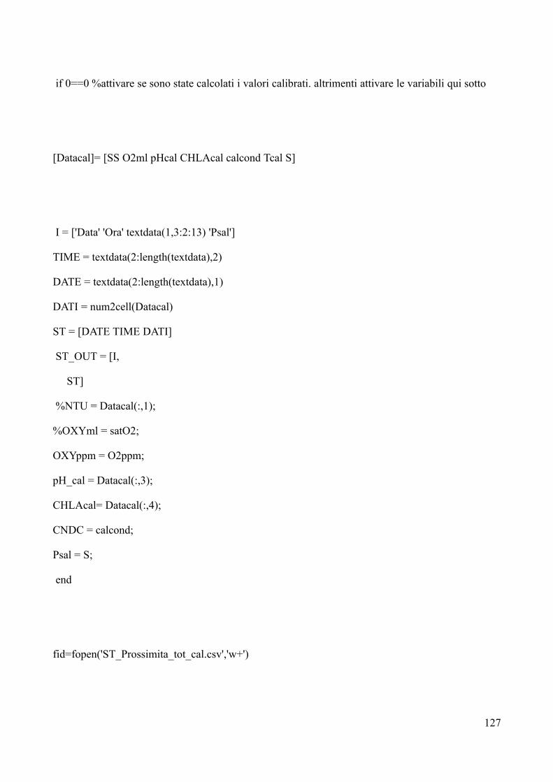
if 0==0 %attivare se sono state calcolati i valori calibrati. altrimenti attivare le variabili qui sotto
[Datacal]= [SS O2ml pHcal CHLAcal calcond Tcal S]
I = ['Data' 'Ora' textdata(1,3:2:13) 'Psal']
TIME = textdata(2:length(textdata),2)
DATE = textdata(2:length(textdata),1)
DATI = num2cell(Datacal)
ST = [DATE TIME DATI]
ST_OUT = [I,
ST]
%NTU = Datacal(:,1);
%OXYml = satO2;
OXYppm = O2ppm;
pH_cal = Datacal(:,3);
CHLAcal= Datacal(:,4);
CNDC = calcond;
Psal = S;
end
fid=fopen('ST_Prossimita_tot_cal.csv','w+')
127

fprintf(fid,'%s, %s, %s, %s, %s, %s, %s, %s,
%s,\n','Date','Time','SS','O2ml','pH_cal','Chl-a_cal','Cond_cal','T_cal','Psal')
for ii=1:length(Data(:,1))
fprintf(fid,'%s, %s, %6.2f, %6.2f, %6.2f, %6.2f, %6.2f, %6.2f,
%6.2f,\n',char(DATE(ii,1)),char(TIME(ii,1)),Datacal(ii,:));
end
fclose(fid)
%Creazione dei grafici
% trasformazione della data e dell'0ra nel fomato serial number per poter essere graficato
MDATE = datevec(DATE, 'dd/mm/yyyy')
MTIME = datevec(TIME, 'HH:MM:SS')
MDAYTIME =[MDATE MTIME]
DAYTIME = [MDAYTIME(:,1) MDAYTIME(:,2) MDAYTIME(:,3) MDAYTIME(:,10)
MDAYTIME(:,11) MDAYTIME(:,12)]
DAYTIME_STR = datestr(DAYTIME)
Tempo=datenum(DAYTIME_STR,0);
%RICHIAMO IL FILE Banchinafig.m PER CREARE I GRAFICI il file si trova nella
%directory TSMALAB della Banchina
Banchinafig
128

=======================================================================
==============================VARSMUT==========================
% programma per smootare i dati di olinda
%importo il file scaricato da olinda e salvato in formato csv e lo processo
%con il file ST_Prox_totalength. Dopo aver eseguito la routine, modificvare
%il nome file di output della presente routin e lanciarla nella finestra di
%comando scrivendo Varsmut. Si ottiene il file delle variabili smutate con
%la funzione smooth(x,y) vedo help online è una cubic spline
% i comandi sotto elencati vengono trascurati se Varsmut è lanciata dopo
% ST_Prox_totalength
%TIME = textdata(2:length(textdata),2) % assegna alla variabile TIME la colonna dell'ora
%DATE = textdata(2:length(textdata),1) % assegna alla variabile DATE la colonna della data
% trasformazione della data e dell'ora nel fomato serial number
%MDATE = datevec(DATE, 'dd/mm/yyyy')
%MTIME = datevec(TIME, 'HH:MM:SS')
%MDAYTIME =[MDATE MTIME]
%DAYTIME = [MDAYTIME(:,1) MDAYTIME(:,2) MDAYTIME(:,3) MDAYTIME(:,10)
MDAYTIME(:,11) MDAYTIME(:,12)]
%DAYTIME_STR = datestr(DAYTIME)
%Tempo=datenum(DAYTIME_STR,0);
129
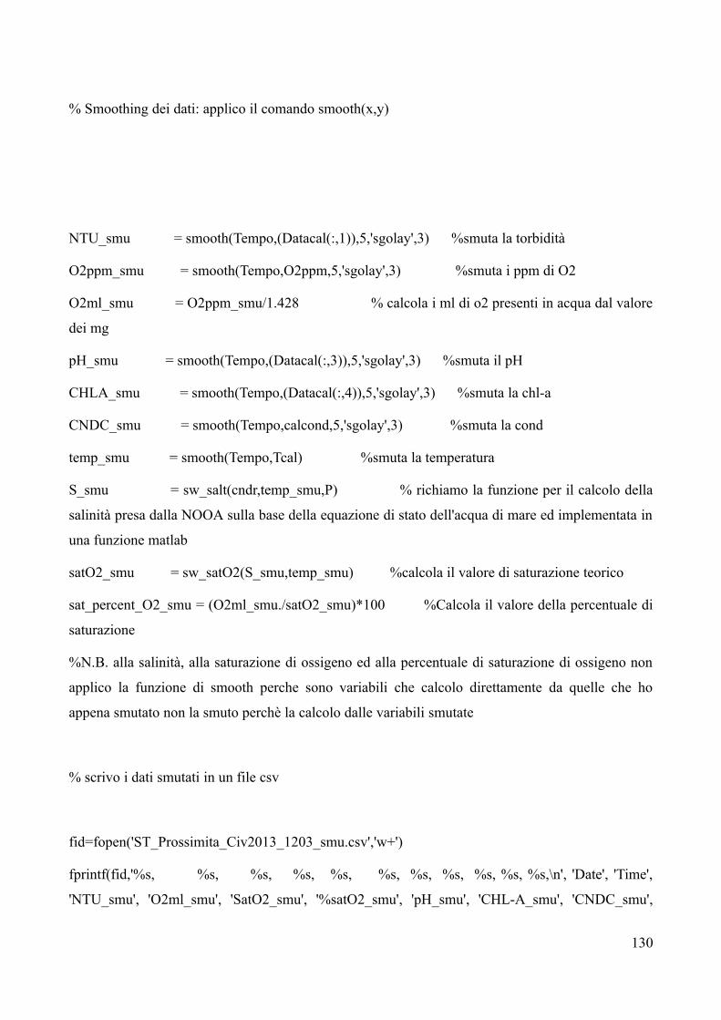
% Smoothing dei dati: applico il comando smooth(x,y)
NTU_smu = smooth(Tempo,(Datacal(:,1)),5,'sgolay',3) %smuta la torbidità
O2ppm_smu = smooth(Tempo,O2ppm,5,'sgolay',3) %smuta i ppm di O2
O2ml_smu = O2ppm_smu/1.428 % calcola i ml di o2 presenti in acqua dal valore
dei mg
pH_smu = smooth(Tempo,(Datacal(:,3)),5,'sgolay',3) %smuta il pH
CHLA_smu = smooth(Tempo,(Datacal(:,4)),5,'sgolay',3) %smuta la chl-a
CNDC_smu = smooth(Tempo,calcond,5,'sgolay',3) %smuta la cond
temp_smu = smooth(Tempo,Tcal) %smuta la temperatura
S_smu = sw_salt(cndr,temp_smu,P) % richiamo la funzione per il calcolo della
salinità presa dalla NOOA sulla base della equazione di stato dell'acqua di mare ed implementata in
una funzione matlab
satO2_smu = sw_satO2(S_smu,temp_smu) %calcola il valore di saturazione teorico
sat_percent_O2_smu = (O2ml_smu./satO2_smu)*100 %Calcola il valore della percentuale di
saturazione
%N.B. alla salinità, alla saturazione di ossigeno ed alla percentuale di saturazione di ossigeno non
applico la funzione di smooth perche sono variabili che calcolo direttamente da quelle che ho
appena smutato non la smuto perchè la calcolo dalle variabili smutate
% scrivo i dati smutati in un file csv
fid=fopen('ST_Prossimita_Civ2013_1203_smu.csv','w+')
fprintf(fid,'%s, %s, %s, %s, %s, %s, %s, %s, %s, %s, %s,\n', 'Date', 'Time',
'NTU_smu', 'O2ml_smu', 'SatO2_smu', '%satO2_smu', 'pH_smu', 'CHL-A_smu', 'CNDC_smu',
130

'Temp_smu', 'Psal_smu')
for ii=1:length(Data(:,1))
fprintf(fid,'%s, %s, %7.3f, %6.3f, %6.3f, %7.3f, %5.3f, %6.3f, %6.3f, %6.3f,
%6.3f,\n',char(DATE(ii,1)),char(TIME(ii,1)), NTU_smu(ii,1), O2ml_smu(ii,1), satO2_smu(ii,1),
sat_percent_O2_smu(ii,1), pH_smu(ii,1), CHLA_smu(ii,1), CNDC_smu(ii,1), temp_smu(ii,1),
S_smu(ii,1));
end
fclose(fid)
plot(Tempo,CNDC, 'k',Tempo,CNDC_smu, 'c')
%plot(Tempo,Tcal, 'k',Tempo,temp_smu, 'r')
%plot(Tempo,S, 'k',Tempo,S_smu, 'y')
%plot(Tempo,CHLAcal, 'k',Tempo,CHLA_smu, 'g')
%plot(Tempo,NTU, 'k',Tempo,NTU_smu, 'm')
%plot(Tempo,satO2, 'b',Tempo,satO2_smu, 'b')
plot(Tempo,Tcal, 'r',Tempo,O2ppm, 'b')
=====================================================================
131


![V.Infrastrutture verdi e blu Sessionesultants [NEP, 2009] “L'infrastruttura verde è una rete, pensata come un progetto di ca-rattere strategico e capace di comprendere la maggior](https://img.pdfslide.tips/doc/110x75/5f0213f77e708231d4027650/vinfrastrutture-verdi-e-blu-sultants-nep-2009-aoelinfrastruttura-verde-una.jpg)