Embed Size (px)
Citation preview
UNIVERSITÉ DU QUÉBEC
MÉMOIRE PRÉSENTÉ À
L'UNIVERSITÉ DU QUÉBEC À TROIS-RIVIÈRES
COMME EXIGENCE PARTIELLE
DE LA MAÎTRISE EN PHYSIQUE
PAR
JULIAN MICHELSEN
HYDROGEN ADSORPTION ON METAL DOPED NANO CARBONS
DÉCEMBRE 2007
Université du Québec à Trois-Rivières
Service de la bibliothèque
Avertissement
L’auteur de ce mémoire ou de cette thèse a autorisé l’Université du Québec à Trois-Rivières à diffuser, à des fins non lucratives, une copie de son mémoire ou de sa thèse.
Cette diffusion n’entraîne pas une renonciation de la part de l’auteur à ses droits de propriété intellectuelle, incluant le droit d’auteur, sur ce mémoire ou cette thèse. Notamment, la reproduction ou la publication de la totalité ou d’une partie importante de ce mémoire ou de cette thèse requiert son autorisation.


Acknowledgemnts
First l would like to thank my director, Prof. Richard Chahine for inviting me to do my
masters at the IRH and making this thesis possible, also giving me great personal sup
port especially when l arrived in Canada. l also thank my principal Dr. Walter Schütz
for sending me to the IRH and his financial support and interest in hydrogen storage.
Furthermore, l would like to thank Dr. Lyubov Lafi for helping me with the essential
chemical pro cesses and Daniel Cossement who assisted me during aIl the time l worked
at the IRH. rd also like to thank Prof. Pierre Bénard for his great help concerning theo
retical problems and aIl the students at the IRH who helped me to find my way through
the UQTR.
This thesis originated out of a collaboration between the Institut de recherche sur l'hydro
gène (IRH) in Trois-Rivières, Canada and FutureCarbon GmbH in Bayreuth, Germany.
The development of the doping procedures used within this thesis as weIl as the improve
ment of sorne characterization methods like the gravimetric and volumetrie method were
performed at the IRH in Canada between September 2005 and May 2006. The investiga
tion of the samples produced was continued at FutureCarbon GmbH in Germany from
June 2006 to October 2007.
l
Summary
Hydrogen storage is the main technological barrier of a viable hydrogen economy. In t he
last decades, different hydrogen storage technologies have been developed and evaluated ,
however , none of t hem has shown a high potent ial for a practical application due to
disadvantages like poor volumetric/ gravimetric st orage capacities, too high or too low
hydrogen binding energies or unappropriate ad/absorption or desorption rates. Recent
research has pointed out an opportunity for the development of a new hydrogen storage
material whose storage effect is based on the interaction between a carbon carrier material
and a metal deposited on its surface. Simulations show a possible hydrogen uptake of
around 8wt % for t itanium doped single-walled nanotubes. Others have shown an increase
of the hydrogen storage capacity of carbon materials by doping them with noble metals
like palladium and platinum.
In this master thesis t he focus lies on the synthesis and characterization of such metal
doped nano-carbons. The metals used for the doping pro cess are t itanium, palladium
and platinum. Different methods like chemical vapor deposition (CVD) and wet-chemical
doping are used to obtain a metal coating on the selected materials. The quality of
the metal coverage is analyzed via X-ray diffraction (XRD) and/ or X-ray photoelectron
spectroscopy (XPS). The hydrogen adsorption capacity of the synthesized samples, is
investigated by volumetrie and gravimetric adsorpt ion measurement methods that were
partly developed within t his thesis. An additional task was to modify an existing Sieverts
apparatus in order to allow the determination of adsorption isotherms at temperatures
lower than 77 K. Therefore, a liquid helium cooling system was developed and installed .
II
As adsorption measurements and imaging techniques on the samples produced show,
the titanium decorated on the surface of the carbon samples tends to oxidize and thus
preventing an adsorption of great amounts of hydrogen. Another difficulty turned out to
be the adjustment of the thickness of the metal layer.
.~
III
Introduction
Le développement d'une économie de l'hydrogène repose sur la mise au point d 'un mode
de stockage efficace et sûr ainsi que d'un système de production à faible coût, ce qui
représente un des grands enjeux actuels. Les systèmes actuels de stockage de l'hydrogène
ne sont pas encore en mesure de concurrencer ceux de stockage traditionnels pétrole
et/ ou gaz, en particulier dans le secteur automobile où la sécurité, l'économie et la fia
bilité d 'un systeme de stockage ainsi que son poids et son prix jouent un rôle important.
L'économie de l'hydrogène étant actuellement considérée comme une alternative possible
à l'économie du pétrole, un apaisement considérable pour l'environnement et une voie
vers une indépendance par rapport au pétrole, des recherches particulièrement intensives
ont lieu en ce qui concerne le stockage de l'hydrogène. Les technologies de stockage uti
lisées dans le domaine de l'automobile pour la mise au point des prototypes tels que le
stockage à haute pression ou sous forme liquide à 20 K dans des réservoirs isolés ther
miquement posent des problèmes pratiques d'utilisation et de commercialisation. On ne
peut atteindre que des densités de stockage volumiques et gravimétriques très basses.
Actuellement, des programmes de recherche se consacrent à la validation de plusieurs
technologies alternatives en ce qui concerne le stockage de l'hydrogène. Parmi ces tech
nologies on compte, en premier lieu, celles utilisant les soit disant hydrures complexes
et hydrures chimiques, un hydrure étant un composé chimique où l'hydrogène a un lien
chimique avec d 'autres éléments. Par exemple en ce qui concerne les hydrures métalli
ques , on a déjà pu atteindre des densités volumiques de stockage très élevées , supérieures
à celle de l'hydrogène liquide. L'inconvénient de cette technologie de stockage est que
1
la dissociation de l'hydrogène, c'est-à-dire son extraction de l'hydrure nécessite beau
coup d 'énergie parce que la liaison chimique est relativement stable (énergie de liaison
d 'environ 80 kJ Imol). En outre, en raison de leur poids élevé, les hydrures métalliques
présentent en général une densité gravimétrique de stockage relativement faible. Une au
tre technologie est en voie de développement; il s'agit de l'adsorption de l'hydrogène à la
surface des matériaux (Sorption). Pendant cette adsorption, les molécules d 'hydrogène
sont liées physiquement par les forces de Van-der-Waals. Les surfaces spécifiques B.E. T
de tels matériaux, par exemple les charbons actifs d'un niveau élevé d'activation, atteig
nent jusqu'à 3000 m2 1 g. La quantité d'hydrogène lié augmente lorsque la température
baisse et lorsque la pression croit; des températures et des pressions autour de 77 K et de
30 bar constituent de bonnes conditions pour l'adsorption physique de l'hydrogène. En
comparaison avec les hydrures complexes et les hydrures chimiques, une simple énergie
de liaison physique d'environ 4 kJ/ mol [1] entraîne une désorption de l'hydrogène, c'est
à-dire un détachement du substrat des molécules absorbées - une légère augmentation
de la température ou une baisse de la pression peut enclencher ce processus. Dans ce cas ,
il est nécessaire de maintenir la température à une valeur aussi basse que possible afin
d'éviter une désorption de l'hydrogène. La solution idéale en ce qui concerne le stockage
de l'hydrogène, par exemple pour une utilisation à bord des voitures, devrait maintenir
l'extraction de l'hydrogène dans une gamme de température située entre 40 oC et 80 oC.
Ces températures pourraient être atteintes grâce à la chaleur dégagée par les cellules de
combustible se trouvant dans la voiture. L'énergie de liaison de l'hydrogène nécessaire
dans ce cas est d 'environ 10 kJ Imol. Les dernières considérations théoriques montrent
que pour certains métaux carbonés, par exemple le titane doté de nanotubes de carbone
2
monofeuillets « SWNT » il est possible d'obtenir des capacités de stockage très élevées
pouvant atteindre 8 wt% [2, 3, 4, 5, 6] cela avec des énergies de liaison très modérées.
On pourrait alors lier 4 molécules d 'hydrogène pro atome de titane en procédant de la
manière suivante: dissocier la première molécule H2 et lier les 3 autres. Un effet sembla
ble en ce qui concerne d'autres métaux pourrait être démontré [7, 8, 9, 10]. La possibilité
d 'adapter l'énergie de liaison dans les matériaux ad/ absorbant de l'hydrogène se trouve
dans le dopage des matériaux de support tels que le carbone avec les métaux [11 , 12, 13,
14]. Dans le présent mémoire, différents systèmes de métaux carbonés sont synthétisés et
analysés par rapport à leur capacité. Cette analyse se concentre sur les métaux suivants
: la platine, le palladium et en plus particulièrement le titane. Comme matériaux de
support , il a été utilisé: le charbon actif IRH 40 fabriqué à l'IRH, les nanomatériaux de
carbone de la société FutureCarbon GmbH comme le « Multi-Walled Carbon Nanotubes
CNT-MW » ainsi que les « Platelet-Nanofibers CNF-PL ».
3
Synthèse des échantillons
Cette partie du document décrit les différents procédés de revêtement des matériaux
carbonés utilisés.
Dopage du titane par procédé dépôt physique et chimique en pha
se vapeur
Le dépôt en phase vapeur est une des possibilités de revêtement d 'un corps solide par un
métal [15, 16, 17, 18]. Le substrat devant recevoir le revêtement est placé dans un réacteur
contenant des vapeurs métalliques. Ici, le matériau qui doit être dopé est introduit dans
un réacteur dont l'atmosphere contient un métal. De cette façon, le métal est déposé sur
l'échantillon grâce à des réactions physiques et/ ou chimiques. Les tests ont été faits avec
du charbon hautement actif comme porteur et du titane comme matériau de dopage.
Un gaz, l'hydrogène ou l'argon est injecté à l'aide d 'un régulateur d'écoulement sur une
petite quantité de tétrachlorure de titane (TiC14 ) dans un tube de verre en quartz dans
lequel on a placé une petite quantité de charbon actif et chauffé par un four. Grâce à
la faible pression exercée par la vapeur dégagée par le tétrachlorure de titane en contact
avec la température ambiante, une certaine quantité du matériau constitutif du dépôt
se libère dans le gaz et réagit physiquement ou chimiquement avec le charbon actif. A
la sortie du four se trouve un bocal d 'eau qui reçoit les gaz échappés afin de protéger
l'environnement. Le PH de cette eau peut être analysé afin de se rendre compte de la
présence ou non des acides. La figure 1 représente le schéma de principe du dispositif
expérimental. Plusieurs expériences ont été menées avec ce dispositif afin de réaliser des
4
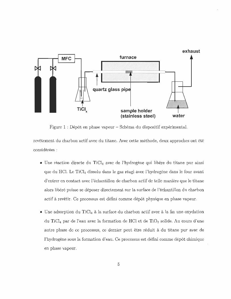
furnace
quartz glass pip
sample holder (stainless steel)
exhaust
water
Figure 1 : Dépôt en phase vapeur - Schéma du dispositif expérimental.
revêtement du charbon actif avec du titane. Avec cette méthode, deux approches ont été
considérées :
• Une réaction directe du TiC14 avec de l'hydrogène qui libère du titane pur ainsi
que du HCL Le TiC14 dissolu dans le gaz réagi avec l'hydrogène dans le four avant
d 'entrer en contact avec l'échantillon de charbon actif de telle manière que le titane
alors libéré puisse se déposer directement sur la surface de l'échantillon du charbon
actif à revêtir. Ce processus est défini comme dépôt physique en phase vapeur.
• Une adsorption du TiC14 à la surface du charbon actif avec à la fin une oxydation
du TiC14 par de l'eau avec la formation de HCl et de Ti02 solide. Au cours d'une
autre phase de ce processus, ce dernier peut être réduit à du titane pur avec de
l'hydrogène sous la formation d'eau. Ce processus est défini comme dépôt chimique
en phase vapeur.
5
Le montage d 'essai a été mis au point à l'Institut de Recherche sur l'Hydrogène (IRH)
et a été reconsidéré en fonction des exigences qui se présentaient. Une série de test a été
pratiquée en utilisant les deux approches citées plus haut. Comme substrat à revêtir, ou
a été utilisé le charbon actif du type IRH 40 à cause de ses bonnes qualités d 'adsorption.
Dopage au titane par le processus chimique humide
D'autres expériences sur le dopage au titane des substrats à base de carbone ont été
réalisées en utilisant un procédé spécial, le processus chimique humide. Par ce procédé,
l'isopropoxide de titane agit comme met al d'apport en libérant du titane losrque du THF
est ajouté. Le titane ainsi libéré peut se déposer sur les surfaces d 'un substrat. Le substrat
à revêtir, le propoxyde de titane et du tetrahydrofurane sont placés dans une ampoule
fermée hermétiquement. L'ensemble du dispositif expérimental est baigné dans de l'huile
qu 'on peut chauffer. Le mélange contenu dans l'ampoule peut être agité à l'aide d'un
agitateur magnétique. Après une période de réaction d'environ deux jours, le propoxyde
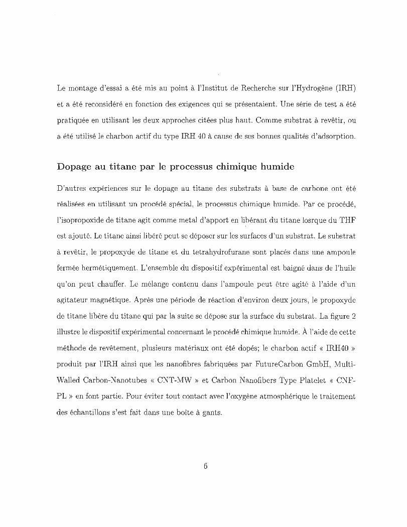
de titane libère du titane qui par la suite se dépose sur la surface du substrat. La figure 2
illustre le dispositif expérimental concernant le procédé chimique humide. À l'aide de cette
méthode de revêtement, plusieurs matériaux ont été dopés; le charbon actif « IRH40 »
produit par l'IRH ainsi que les nanofibres fabriquées par FutureCarbon GmbH, Multi
Walled Carbon-Nanotubes « CNT-MW » et Carbon Nanofibers Type Platelet « CNF
PL » en font partie. Pour éviter tout contact avec l'oxygène atmosphérique le traitement
des échantillons s'est fait dans une boîte à gants.
6
thermometer
condenser
titaniumisopropoxide
oil bath + THF
\ magnetic stirrer sam pie (powder)
Figure 2 : Processus chimique humide - Schéma du dispositif expérimental
Dopage au platine/palladium par le processus chimique humide
Avec cette méthode, le revêtement est produit par une décomposition thermique d'un
précurseur métallifère placé dans une solution [19]. L'induction se fait à des fréquences
micro-ondes. Dans cette méthode, la solution contenue dans le précurseur ainsi que le
matériau de carbone à revêtir sont chauffés à l'aide des fréquences micro-ondes. En raison
de la conductivité électrique élevée du matériau carboné, une surchauffe partielle à sa
surface est obtenue, ce qui entraîne une décomposition et donc une séparation locale du
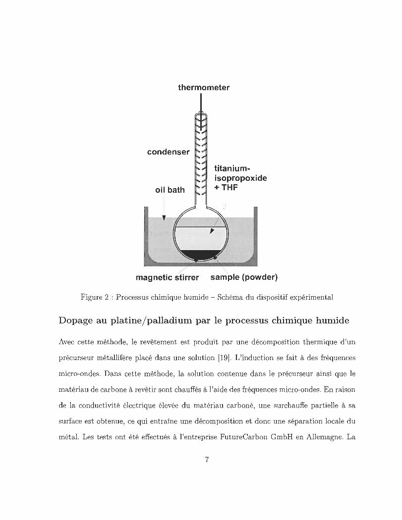
métal. Les tests ont été effectués à l'entreprise FutureCarbon GmbH en Allemagne. La
7
figure 3 montre le dispositif expérimental développé chez FutureCarbon GmbH.
Figure 3 : Dispositif expérimental pour le revêtement des matériaux carbonés par microondes.
8
Caractérisation des échantillons synthétisés.
Dans cette étude, la capacité de stockage de l'hydrogène a été déterminée par des métho
des de mesures volumétrique ainsi que gravimétrique. Pour prouver la présence les dépôts
métalliques sur les matériaux à revêtir, la diffractométrie aux rayons X (XRD) ainsi que
la spectrométrie de photo électrons X (XPS) ont également été utilisées.
Mesure volumétrique de la capacité de stockage.
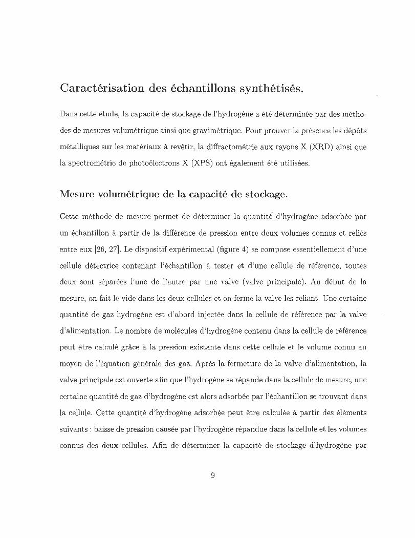
Cette méthode de mesure permet de déterminer la quantité d'hydrogène adsorbée par
un échantillon à partir de la différence de pression entre deux volumes connus et reliés
entre eux [26, 27]. Le dispositif expérimental (figure 4) se compose essentiellement d 'une
cellule détectrice contenant l'échantillon à tester et d'une cellule de référence, toutes
deux sont séparées l'une de l'autre par une valve (valve principale). Au début de la
mesure, on fait le vide dans les deux cellules et on ferme la valve les reliant. Une certaine
quantité de gaz hydrogène est d'abord injectée dans la cellule de référence par la valve
d 'alimentation. Le nombre de molécules d'hydrogène contenu dans la cellule de référence
peut être calculé grâce à la pression existante dans cette cellule et le volume connu au
moyen de l'équation générale des gaz. Après la fermeture de la valve d 'alimentation, la
valve principale est ouverte afin que l'hydrogène se répande dans la cellule de mesure , une
certaine quantité de gaz d'hydrogène est alors adsorbée par l'échantillon se trouvant dans
la cellule. Cette quantité d 'hydrogène adsorbée peut être calculée à partir des éléments
suivants: baisse de pression causée par l'hydrogène répandue dans la cellule et les volumes
connus des deux cellules. Afin de déterminer la capacité de stockage d 'hydrogène par
9
Pressure Gauge
Gas input
Measuring cell ---Iq:.<, Reference cell
Sample
LN2-Dewar
Figure 4 : Montage typique d 'un appareillage de mesure volumétrique composé de volumes à mesurer et de volumes de référence séparés l'un de l'autre par la valve principale.
la méthode de mesure volumétrique, deux systèmes de mesure automatiques différents
étaient disponibles à l'Institut de Recherche sur l'Hydrogène (IRH), en l'occurrence des
systèmes de mesure suivants: « Autosorb-1 » de l'entreprise « QUANTACHROME » et
« ASAP 2020 » de l'entreprise « MICROMERITICS ». Les deux systèmes permettant de
faire des mesures dans la gamme de température allant de 77 K à 295 K avec des pressions
pouvant atteindre 1 bar. Pour permettre également des mesures avec une température
de 77 K et des pressions pouvant atteindre 40 bar, un système de mesure volumétrique
de l'entreprise FutureCarbon GmbH a été mise au point.
10
Mesures gravimétriques de la capacité de stockage
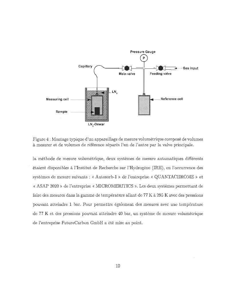
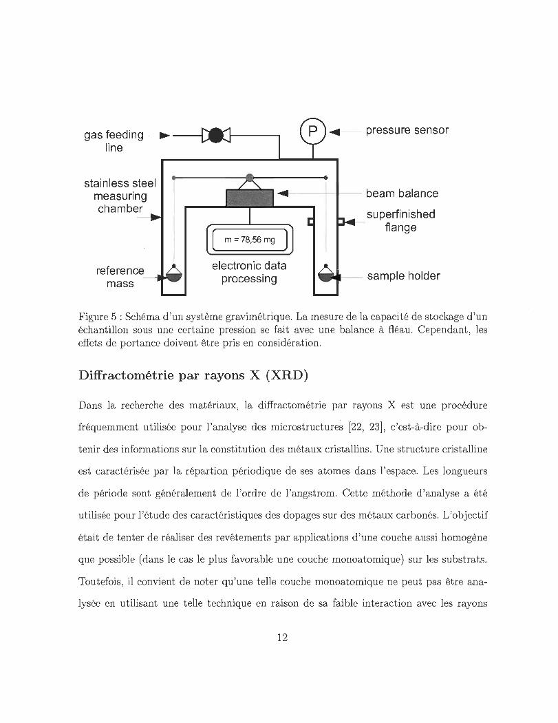
Une autre manière de déterminer la quantité d'hydrogène adsorbée par un échantillon,
c'est la méthode de mesure gravimétrique [26, 28, 29]. Dans cette méthode le poids de
l'échantillon à tester, celui-ci se trouvant dans une cellule de mesure fermée, est mesuré
par une balance de précision. Avant de commencer la mesure, on fait le vide dans la cel
lule de mesure et ensuite on la remplit d'hydrogène. Une augmentation de poids est alors
constatée sur la balance de précision due à l'adsorption d'hydrogène par l'échantillon.
Cependant, l'augmentation de poids indiquée par la balance de précision ne correspond
pas à la quantité totale adsorbée car la mesure est influencée par des effets de flottabilité
qui doivent être additionnés par la suite pour déterminer la vrai quantité d 'hydrogène ab
sorbée. Les paramètres de flottabilité peuvent être déterminés par une mesure à l'hélium
en raison de son adsorption négligeable sur l'échantillon. Les effets de flottabilité peuvent
ainsi être calculés directement. La figure 5 illustre un schéma de principe du dispositif
mesure gravimétrique. Pour pouvoir effectuer des mesures de capacité gravimétriques
l'IRH a mis au point un système qui permet des mesures à la température ambiante et
sous une pression maximale de 100 bar. Les échantillons à mesurer avaient une masse
de l'ordre de 100 mg, la résolution de la balance à fléau utilisée dans cet appareillage de
mesure Type « CahnD410 » était de 10 fJ,g. En comparaison avec ceux utilisés pour les
mesures volumétriques, ce dispositif a permis d'atteindre une résolution très élevée même
sous haute pression.
11
gas feeding ------.----1 ~-- pressu re sensor
line.
stainless steel measuring cham ber
~----------t--.--- beam balance
reference -~-mass
( m = 78,56 mg )
electronic data processing
superfinished Lr'IIIII_ fi a n 9 e
.... -- sample holder
Figure 5 : Schéma d'un système gravimétrique. La mesure de la capacité de stockage d'un échantillon sous une certaine pression se fait avec une balance à fléau. Cependant, les effets de portance doivent être pris en considération.
Diffractométrie par rayons X (XRD)
Dans la recherche des matériaux, la diffractométrie par rayons X est une procédure
fréquemment utilisée pour l'analyse des microstructures [22, 23], c'est-à-dire pour ob-
tenir des informations sur la constitution des métaux cristallins. Une structure cristalline
est caractérisée par la répartion périodique de ses atomes dans l'espace. Les longueurs
de période sont généralement de l'ordre de l'angstrom. Cette méthode d'analyse a été
utilisée pour l'étude des caractéristiques des dopages sur des métaux carbonés. L'objectif
était de tenter de réaliser des revêtements par applications d'une couche aussi homogène
que possible (dans le cas le plus favorable une couche monoatomique) sur les substrats.
Toutefois, il convient de noter qu'une telle couche monoatomique ne peut pas être ana-
lysée en utilisant une telle technique en raison de sa faible interaction avec les rayons
12
X. L'apparition d 'un pic dans le diagramme du diffractogramme révèle l'existence d'une
couche multimoléculaire.
Spectrométrie de photoélectrons induit par rayons X (XPS)
La XPS est basé sur l'effet photoélectrique extérieur, par lequel des photoélectrons sont
libérés de l'échantillon sous l'effet de rayonnements électromagnétiques [24, 25]. La déter
mination de l'énergie cinétique de ces électrons (spectroscopie) permet de tirer des conclu
sions sur la composition chimique et la constitution électronique de l'échantillon analysé.
Le XPS compte aujourd 'hui parmi les méthodes les plus utilisées dans la physique des
solides ainsi que dans d'autres domaines voisins comme la physique des surfaces et la
science des matériaux pour l'analyse de la structure électronique d'un matériau donné.
Cette méthode de caractérisation permet une analyse de surface d 'un échantillon afin
de déterminer le type de matériaux se trouvant sur sa surface ainsi que de leur état de
liaison. Contrairement à la méthode déjà présentée - diffractométrie de rayon X - des
couches monoatomiques peuvent aussi être dét ectées.
13
Résultats
Dans cette section les résultats des différentes méthodes de caractérisation sont présentés,
évalués et commentés.
Diffractométrie par rayons X - Résultats
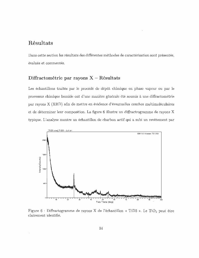
Les échantillons traités par le procédé de dépôt chimique en phase vapeur ou par le
processus chimique humide ont d'une manière générale été soumis à une diffractométrie
par rayons X (XRD) afin de mettre en évidence d'éventuelles couches multimoléculaires
et de déterminer leur composition. La figure 6 illustre un diffractrogramme de rayons X
typique. L'analyse montre un échantillon de charbon actif qui a subi un revêtement par
086-11 57> Anatase - 110.7202
2000
1500
10 20 30 40 50 60 70 80 90 100
Two-Theta (deg)
Figure 6 : Diffractogramme de rayons X de l'échantillon « TiD3 ». Le Ti02 peut être clairement identifié.
14
le procédé dépôt chimique en phase vapeur. Ici le TiC14 a d'abord été adsorbé puis réduit
en Ti02 , ce dernier a ensuite été exposé à l'hydrogène pour ainsi obtenir du titane pur
sur la surface de l'échantillon. Dans le diffractogramme, la présence de dioxyde de titane
(Ti02 ) qui apparaît dans des agglomérats dont le diamètre est au minimum équivalent à
celui de 100 molécules est clairement visible. Il y a 2 interprétations possibles en ce qui
concerne la présence de Ti02 :
• Le revêtement du charbon actif avec le titane s'est d'abord déroulé avec succès.
Après le processus de revêtement le titane se trouvant sur l'échantillon s'est oxydé
dans la boîte à gants à cause de la grande reactivité de l'échantillon .
• La réduction de Ti02 à partir d'hydrogène dans le four de verre en quartz n 'a pas
réussie parce que la température n'était pas suffisamment élevée ou pour d'autres
raIsons.
Spectrométrie de photoélectrons induits par rayons X - Résultats
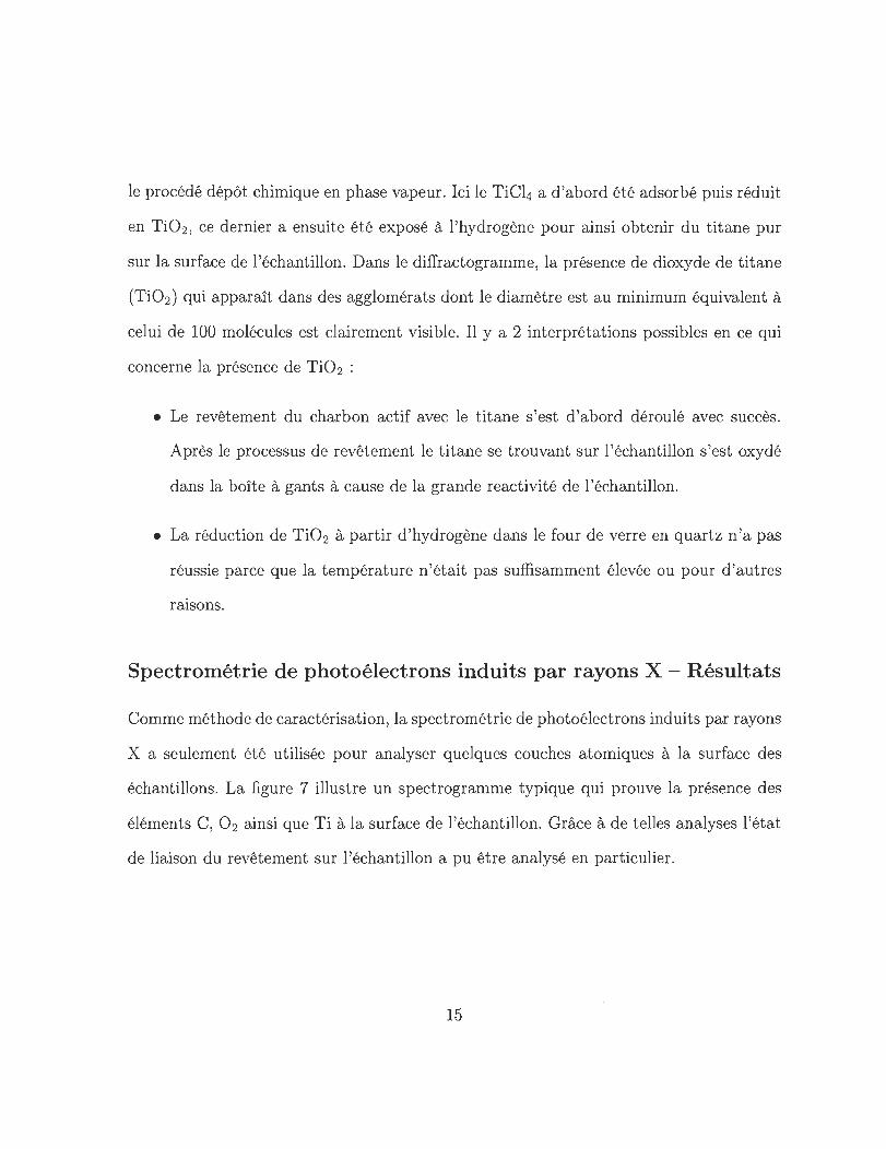
Comme méthode de caractérisation, la spectrométrie de photo électrons induits par rayons
X a seulement été utilisée pour analyser quelques couches atomiques à la surface des
échantillons. La figure 7 illustre un spectrogramme typique qui prouve la présence des
éléments C, O2 ainsi que Ti à la surface de l'échantillon. Grâce à de telles analyses l'état
de liaison du revêtement sur l'échantillon a pu être analysé en particulier.
15
TiD3
45~~---------------------------------------------'
CIl 0.. U
40
35
30
25
20
15
10
Name P05. FWHM Area At% o 15 532. 15 6.364 8677. 1 25.951 C 15 285.43 3.526 84 15.6 73.745 Ti 2p 459.42 2.274 270.9 0.304
1200 1000 800
o
600 Binding Energy (eV)
u
400 200
Figure 7 : XPS spectrogramme de l'échantillon « TiD3 »
Capacité d'adsorption - Résultats
o
L'influence sur la capacité de stockage de l'hydrogène d 'un matériau de stockage à base
de carbone et revêtu de métal, ne peut finalement être caractérisée qu'avec une mesure
de capacité directe et ainsi être comparée à des matériaux qui n 'ont pas subi de revête-
16
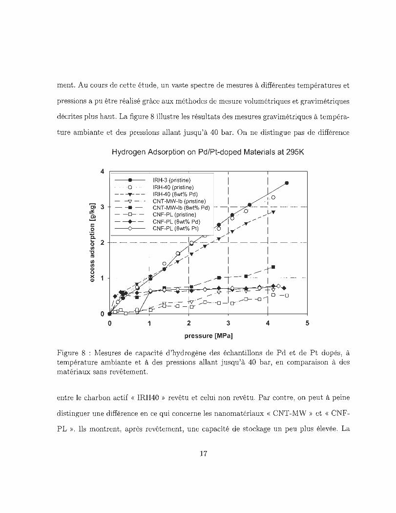
ment. Au cours de cette étude, un vaste spectre de mesures à différentes températures et
pressions a pu être réalisé grâce aux méthodes de mesure volumétriques et gravimétriques
décrites plus haut . La figure 8 illustre les résultats des mesures gravimétriques à tempéra-
t ure ambiante et des pressions allant jusqu 'à 40 bar. On ne distingue pas de différence
4
Ci 3 ~ -Cl ....... s:::: o .. a. o 2 1/) 1j C'tI 1/) 1/) (1) (J
~ 1
Hydrogen Adsorption on Pd/Pt-doped Materials at 295K
• o
---T---- -v - . ----- -0- .----+-----0---
IRH-3 (pristine) IRH-40 (pristine) IRH-40 (8wt% Pd) CNT-MW-Ib (pristine) CNT-MW-Ib (8wt% Pd) CNF-PL (pristine) CNF-PL (8wt% Pd) CNF-PL (8wt% Pt)
.. t 0 -L-... --
x""''''''''''' 1
j....- "'" 1
___ 1_ - - - 1 ~ -""--'t"~I _ - - ---J- --·I ..... ~ 1 1
..... T
o /~ 1 1 1
1", 1 1 .- -r---7' ---I--.-~-=-----l---
.-- .V" + - . T ..
-- D-O 1 - - +v -:0- -a _10---0- -01 ty ::::5-= {] - 0- 1
o~~~~+-------+-------+-------~----~
o 1 2 3 4 5
pressure [MPaJ
Figure 8 : Mesures de capacité d 'hydrogène des échantillons de Pd et de P t dopés, à température ambiante et à des pressions allant jusqu 'à 40 bar, en comparaison à des matériaux sans revêtement.
entre le charbon actif « IRH40 » revêtu et celui non revêtu. Par contre, on peut à peine
distinguer une différence en ce qui concerne les nanomatériaux « CNT -MW » et « CNF
P L ». Ils montrent , après revêtement , une capacité de stockage un peu plus élevée. La
17
quantité d'hydrogène stockée en plus par les nanomatériaux ayant subi un revêtement
peut s'expliquer par la formation d'un hydrure métallique.
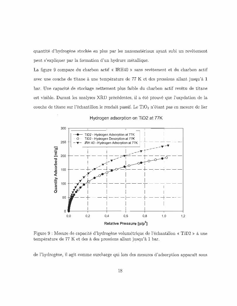
La figure 9 compare du charbon actif « IRH40 » sans revêtement et du charbon actif
avec une couche de titane à une température de 77 K et des pressions allant jusqu'à 1
bar. Une capacité de stockage nettement plus faible du charbon actif revêtu de titane
est visible. Durant les analyses XRD précédentes, il a été prouvé que l'oxydation de la
couche de titane sur l'échantillon le rendait passif. Le Ti02 n'étant pas en mesure de lier
Hydrogen adsorption on TiD2 at 77K
300 ~------~------~----~------~------~------~
250
...... C) -l 200
"0 al ..c .... ~ 150
~ ~ += 1: 100 ni ::J o
50
-----...- TiD2 - Hydrogen Adsorption at 77K 1
l __ ~ __ _ ---~-...
-0 TiD2 - Hydrogen Desorption at 77K - .... - IRH 40 - Hydrogen Adsorption at 77K
--.... ..:.-- 1
'1'/('1'/>""'1'/:::'" - T - - c:t - --
1 /'.
--+~--+ ~ i ! i 1
yT ; i ; ; 1
~ T--~---~--i--l------ --+---f---
1
o __ ------+-------~------~----~------_4------~ 0,0 0,2 0,4 0,6 0,8 1,0 1,2
Relative Pressure [p/pO]
Figure 9 : Mesure de capacité d 'hydrogène volumétrique de l'échantillon « TiD2 » à une tempèrature de 77 K et des à des pressions allant jusqu'à 1 bar.
de l'hydrogène, il agit comme surcharge qui lors des mesures d'adsorption apparaît sous
18
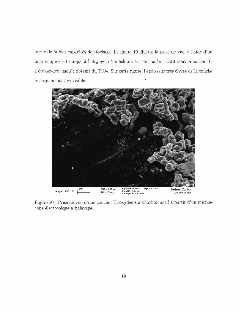
forme de faibles capacités de stockage. La figure 10 illustre la prise de vue, à l'aide d 'un
microscope électronique à balayage, d'un échantillon de charbon actif dont la couche-Ti
a été oxydée jusqu'à obtenir du Ti02 . Sur cette figure , l'épaisseur très élevée de la couche
est également très visible.
1~m·
Mag = 10.00 K X I-I----i EHT · ~.OO kV WO - 2mm
Sign.1 A- loLenl Signa.l - 1.000 Signai B • InLens File Name. TiD5_05.trt
Future Carbon Dite :26 Sep 2007
Figure 10 : Prise de vue d 'une couche -Ti oxydée sur charbon actif à partir d 'un microscope électronique à balayage.
19
Résumé.
En conclusion ont peut résumer:
• Les processus visant le revêtement des échantillons carbonés avec des métaux se
sont déroulés pour la plus grande partie avec succès. Dans tous les cas, ces métaux
on pu être déposés sur les échantillons. Un affinage de certains paramètres a permis
de jouer sur l'épaisseur des couches, assez élevée au début et cela en particulier pour
le procédé dépôt physique. Finalement, ce sont les méthodes chimiques humides qui
se sont avérées comme étant les méthodes les mieux contrôlables lors d'un processus
de revêtement.
• Le plus grand problème a été l'oxydation de la couche de titane. Même en stockant
les échantillons dans une boîte à gants, le titane s'est oxydé avec le reste d'oxygène
s'y trouvant. Une réduction du Ti02 à un Ti brut n'a pas pu se faire.
• Les échantillons revêtus de métaux précieux Pt et Pd ont montré une capacité de
stockage un peu plus élevée qui peut toutefois s'expliquer par la formation d 'un
hydrure métallique.
D'autres travaux pourraient viser une amélioration de la méthode de revêtement chimique
humide. En ce qui concerne d'autres recherches avec des échantillons revêtus de Ti , une
atmosphère absolument interne est indispensable. Dans le meilleur des cas, la synthèse et
la caractérisation devraient être effectuées dans une boîte à gants de sorte que le transport
des échantillons synthétisés puisse être supprimé.
20
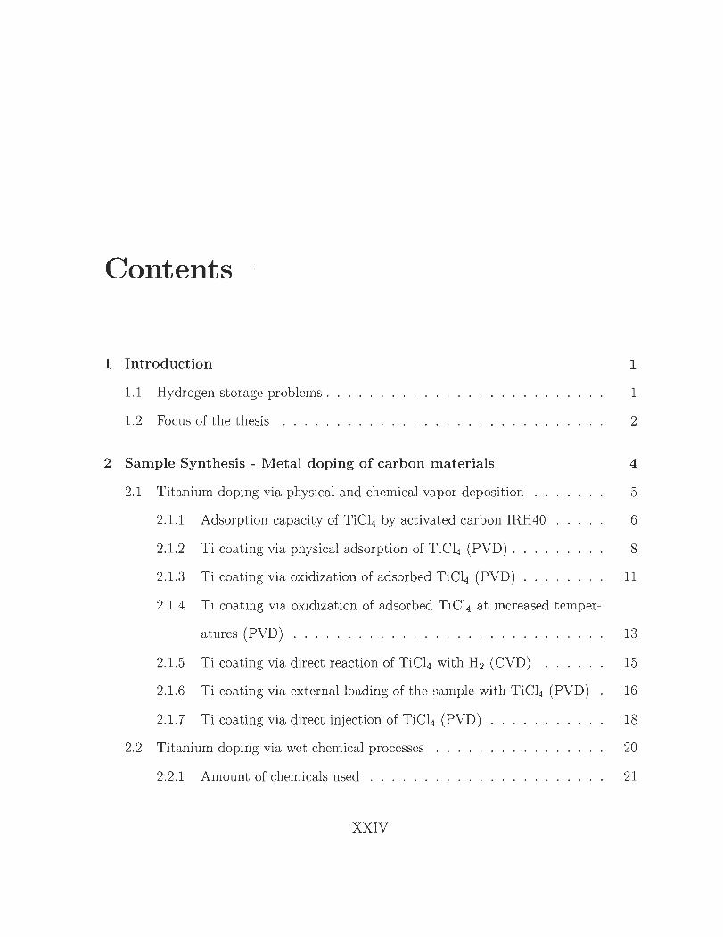
Contents
1 Introduction
1.1 Hydrogen storage problems .
1.2 Focus of the thesis ... . .
2 Sample Synthesis - Metal doping of carbon materials
2.1 Titanium doping via physical and chemical vapor deposition
2.1.1 Adsorption capacity of TiC14 by activated carbon IRH40
2.1.2 Ti coating via physical adsorption of TiC14 (PVD) .
1
1
2
4
5
6
8
2.1.3 Ti coating via oxidization of adsorbed TiC14 (PVD) 11
2.1.4 Ti coating via oxidization of adsorbed TiC14 at increased temper-
atures (PVD) . . . . . . . . . . . . . . . . . . . . . . . 13
2.1.5 Ti coating via direct reaction of TiC14 with H2 (CVD) 15
2.1.6 Ti coating via externalloading of t he sample with TiC14 (PVD) 16
2.1.7 Ti coating via direct injection of TiC14 (PVD) 18
2.2 Titanium doping via wet chemical pro cesses
2.2.1 Amount of chemicals used . . . . . .
XXIV
20
21
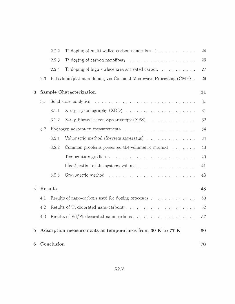
2.2.2
2.2.3
Ti doping of multi-walled carbon nanotubes
Ti doping of carbon nanofibers ...... .
24
26
2.2.4 Ti doping of high surface area activated carbon 27
2.3 Palladium/ platinum doping via Colloidal Microwave Processing (CMP) 29
3 Sample Characterization 31
3. 1 Solid state analytics ....... . 31
3. 1.1 X-ray crystallography (XRD) 31
3. 1.2 X-ray Photoelectron Spectroscopy (XPS) 32
3.2 Hydrogen adsorption measurements ...... .
3.2.1 Volumetrie method (Sieverts apparatus)
3.2.2 Common problems presented t he volumetrie method
Temperature gradient . . . . . . . . .
Identification of t he systems volume .
3.2.3 Gravimetrie method . . ...... .
4 Results
4.1 Results of nano-carbons used for doping pro cesses
4.2 Results of Ti decorated nano-carbons ...
4.3 Results of Pd/ Pt decorated nano-carbons .
34
34
40
40
41
43
48
50
52
57
5 Adsorption measurements at temperatures from 30 K to 77 K 60
6 Conclusion 70
XXV
Appendix 73
A XRD results 73
B XPS results 84
C Hydrogen adsorption measurements 93
XXVI
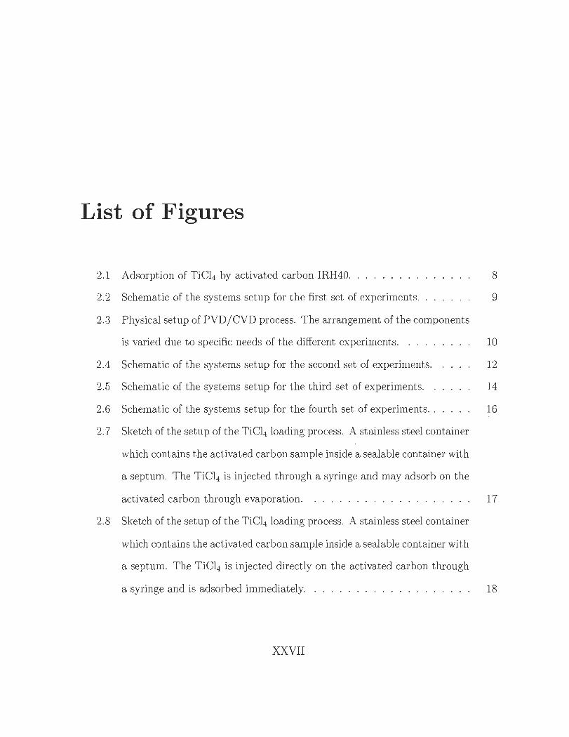
List of Figures
2.1 Adsorption of TiC14 by activated carbon IRH40. . . . . . . . .
2.2 Schematic of the systems setup for the first set of experiments.
2.3 Physical setup of PVD /CVD process. The arrangement of the components
8
9
is varied due to specifie needs of the different experiments. . . . . 10
2.4 Schematic of the systems setup for the second set of experiments. 12
2.5 Schematic of the systems setup for the third set of experiments. . 14
2.6 Schematic of the systems setup for the fourth set of experiments. . 16
2.7 Sketch of the setup of the TiC14 loading process. A stainless steel container
which contains the activated carbon sample inside a sealable container with
a septum. The TiCl4 is injected through a syringe and may adsorb on the
activated carbon through evaporation. ................... 17
2.8 Sketch of the setup of the TiCl4 loading process. A stainless steel container
which contains the activated carbon sample inside a sealable container with
a septum. The TiCl4 is injected directly on the activated carbon through
a syringe and is adsorbed immediately. . . . . . . . . . . . . . . . . . .. 18
XXVII
2.9 Typical setup of the wet chemical pro cess showing the ftask containing the
liquid solution and the carbonaceous sample with the condenser mounted
on the top. A thermometer allows the observation of the temperature
provided by a heating plate which heats the oil bath the ftask is located
in. The sketch does not show the aluminum foil wrapped around the setup
to prevent radiation contacting the chemical solution. . . . . . . . . . .. 20
2.10 Model of a tetra-hydrofuran molecule. Red: oxygen, black: carbon, blue
: hydrogen . . . . . . . . . . . . . . . . . . . . . . . . . . . . . . . . . .. 24
2.11 SEM/ TEM image of mult i-walled carbon nanotubes MWNT-Ib produced
by FutureCarbon. . . . . . . . . . . . . . . . . . . . . . . . . . . .. . . .. 25
2.12 SEM/ TEM image of carbon nanofibers CNF-P L produced by FutureCarbon. 26
2.13 Colloidal Microwave Processing (CMP) experimental setup.. . . . . . .. 29
3.1 Typical setup of a volumetrie measurement system (Sieverts apparatus)
showing two volumes (measuring volume and reference volume) separated
by the main valve. Through gas expansion from the reference volume
into the measuring volume, the hydrogen adsorption capacity of a sample
located in the measuring cell can be determined through the pressure drop
caused by the gas expansion. . . . . . . . . . . . . . . . . . . . . . . 35
3.2 Volumetrie test bed at FutureCarbon GmbH in Bayreuth, Germany. The
test bed is designed for the measurement of adsorption isotherms of sam
pIes with a mass up to 10 g at temperatures ranging from 77 K to 500 K
and pressures up to 100 bar. . . . . . . . . . . . . . . . . . . . . . . . .. 36
XXVIII
3.3 Photo of the beam balance type Cahn D410 used for the gravimetric
experiments . . . . . . . . . . . .
3.4 Sketch of a gravimetric measurement system. The hydrogen adsorption
at a certain pressure can be determined through the mass measured by
the balance minus the buoyancy of the sample caused by the surrounding
44
hydrogen gas. . . . . . . . . . . . . . . . . . . . . . . . . . . . . . . . .. 45
3.5 Gravimetrie setup at the IRH allowing measurements at pressures up to
100 bar. . . . . . . . . . . . . . . . . . . . . . . . . . . . . . . . . . . .. 46
4.1 (TiD3) Formation of Ti02 on the surface of activated carbon. 53
4.2 (TiD5) Formation of different metals on the surface of the activated carbon
sample.. . . . . . . . . . . . . . . . . . . . . . . . . . . . . . . . . . . .. 54
4.3 (TiD6) Formation of nano-scaled Ti0 2 on the surface of the activated
carbon sample. ............ .. ............... 55
4.4 (TiLl) Formation of Ti0 2 on the surface of multi-walled nanotubes. 56
4.5 (TiL3) Formation of Ti02 on the surface of activated carbon particles. An
SE-detector was used for the imaging process to highlight the metal content . 57
A.l XRD spectrum of activated carbon IRH40 doped with 8wt% Pd showing
the peaks related to Pd. . . . . . . . . . . . . . . . . . . . . . . . . . .. 74
A.2 XRD spectrum of carbon nanotubes CNT-MW 'as synthesized' showing
the peaks related to Co. . . . . . . . . . . . . . . . . . . . . . . . . . .. 75
A.3 XRD spectrum of carbon nanofibers CNF-PL 'as synthesized' showing the
peaks related to C. . . . . . . . . . . . . . . . . . . . . . . . . . . . . . . 75
XXIX
A.4 XRD spectrum of carbon nanofibers CNF-PL 'as synthesized' showing the
peaks related to Fe3C. . . . . . . . . . . . . . . . . . . . . . . . . . . .. 76
A.5 XRD spectrum of carbon nanofibers CNF-PL doped with 8wt% Pd show-
ing the peaks related to C. . . . . . . . . . . . . . . . . . . .
A.6 XRD spectrum of TiD2 showing the peaks related to Ti02 ..
A.7 XRD spectrum of TiD3 showing the peaks related to Ti02 ..
A.8 XRD spectrum of TiD3 showing the peaks related to TiH2 . .
A.9 XRD spectrum of TiD5 showing the peaks related to NiFe .
A.lO XRD spectrum of TiD5 showing the peaks related to Cr F e.
A.11 XRD spectrum of TiD5 showing the peaks related to Ti02 ..
A.12 XRD spectrum of TiLl showing the peaks related to Ti02 .
A.13 XRD spectrum of TiLl showing the peaks related to TiCs.
A.14 XRD spectrum of TiLl showing the peaks related to TiC.
A.15 XRD spectrum of TiLl showing the peaks related to Ti .
A.16 XRD spectrum of TiL2 showing the peaks related to Ti.
A.17 XRD spectrum of TiL2 showing the peaks related to Ti 20 3 .
A.18 XRD spectrum of TiL2 showing the peaks related to Ti0 2 ..
B.l XPS spectrum of TiD3 showing 3 emission lines for titanium, oxygen and
carbon ... . .... .. . . ............ . ... .
B.2 XPS spectrum of TiD3 with focus on emission line Ti 2s.
B.3 XPS spectrum of TiD3 with focus on emission line Ols.
B.4 XPS spectrum of TiD3 with focus on emission line Ti 2p.
xxx
76
77
77
78
78
79
79
80
80
81
81
82
82
83
85
86
87
88
B.5 XPS spectrum of TiD3 with focus on emission line C l s. . . . . . . . . S9
B.6 XPS spectrum of TiD4 showing 2 emission lines for oxygen and carbon. 90
B.7 XPS spectrum of TiD4 with focus on emission line Ols. 91
B.S XPS spectrum of TiD4 with focus on emission line C ls. 92
C.1 Hydrogen adsorption measurements performed with the gravimetric mea
surement system at a temperature of 295 K and pressures up to 4 MPa.
Samples shown are Pd and Pt covered carbon materials in comparison
with their undoped pristine materials. . . . . . . . . . . . . . . . . . . .. 94
C.2 Hydrogen adsorption measurements performed with the gravimetric mea
surement system at a temperature of 295 K and pressures up to 4 MPa.
Samples shown are Ti covered carbon materials in comparison with their
undoped pristine materials. .. .. ... .... ... .. ... . . . .. . 95
C.3 Hydrogen adsorption measurements performed with the volumetrie mea
surement system at a temperature of 77 K and pressures up to 1 bar.
Sample shown is the activated carbon IRH40. .... .. ... . . 96
C.4 Hydrogen adsorption measurements performed with the volumetrie mea
surement system at a temperature of 295 K and pressures up to 1 bar.
Sample shown is the activated carbon IRH40. ........... 97
C.5 Hydrogen adsorption measurements performed with the volumetrie mea
surement system at a temperature of 77 K and pressures up to 1 bar.
Sample shown is the Ti covered sample TiD2 in comparison with its pris-
t ine material IRH40. . . . . . . . . . . . . . . . . . . . . . . . . . . . .. 9S
XXXI
Co6 Hydrogen adsorption measurements performed with the volumetrie mea
surement system at a temperature of 295 K and pressures up to 1 bar.
Sample shown is the Ti eovered sample TiD2 in eomparison with its pris-
t ine material IRH 400 0 0 0 0 0 0 0 0 0 0 0 0 0 0 0 0 0 0 0 0 0 0 0 0 0 0 0 0 0 99
Co 7 Hydrogen adsorption measurements performed with the volumetrie mea
surement system at a temperature of 77 K and pressures up to 1 bar.
Sample shown is the Ti eovered sample TiLl in eomparison with its pris-
tine material CNT-MWo 0 0 0 0 0 0 0 0 0 0 0 0 0 0 0 0 0 0 0 0 0 0 0 0 0 0 0 100
Co8 Hydrogen adsorpt ion measurements performed with the volumetrie mea
surement system at a temperature of 77 K and pressures up to 1 bar.
Sample shown is the Ti eovered sample TiL3 in eomparison with its pris-
t ine material IRH400 0 0 0 0 0 0 0 0 0 0 0 0 0 0 0 0 0 0 0 0 0 0 0 0 0 0 0 0 0 101
XXXII
List of Tables
2.1 Explanation to the Dubinin-Raduskevitch relation 6
2.2 Properties of Titanium iso-propoxide 22
2.3 Properties of tetra-hydrofuran . . . . 23
2.4 Properties of multi-walled carbon nanotubes MWNT-Ib produced by Fu-
tureCarbon . . . . . . . . . . . . . . . . . . . . . . . . . . . . . . . . 24
2.5 Properties of carbon nanofibers CNF-PL produced by FutureCarbon. 26
4.1 List of pristine materials, their pretreatments and analysis. . . 48
4.2 List of metal doped samples, their pretreatments and analysis. 49
XXXIII
Chapter 1
Introduction
1.1 Hydrogen st orage problems
The development of a functional and economical hydrogen storage system is a key issue
for a working hydrogen economy. Unlike gasoline, hydrogen is gaseous at room tempera
ture and diffuses t hrough tank hulls due to its small molecular size which complicates its
efficient storage. Commonly used storage technologies like high pressure tanks or liquid
hydrogen storage systems are quite well developed but still show unacceptable char acter
istics in energy density, economy and complexity for practical applications. Beside t he
storage of hydrogen in gaseous or liquid states, another possibility is to let the hydrogen
interact with a solid material in order t o bind to the surface or its molecular grid.
In the last decades, a lot of research has been aimed at the development of an adequate
material for this type of hydrogen storage. However , a suit able material has not been
found yet. One of the major characteristics of such a material is its sorpt ion enthalpy.
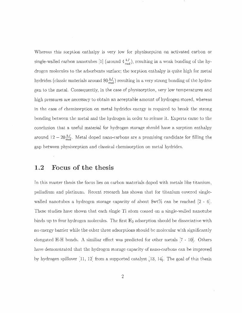
Whereas this sorption enthalpy is very low for physisorption on activated carbon or
single-walled carbon nanotubes [1] (around 4!~z)' resulting in a weak bonding of the hy
drogen molecules to the adsorbents surface; the sorption enthalpy is quite high for metal
hydrides (classic materials around 80 !~z) resulting in a very strong bonding of the hydro
gen to the metal. Consequently, in the case of physisorption, very low temperatures and
high pressures are necessary to obtain an acceptable amount of hydrogen stored, whereas
in the case of chemisorption on metal hydrides energy is required tQ break the strong
bonding between the metal and the hydrogen in or der to release it. Experts came to the
conclusion that a useful material for hydrogen st orage should have a sorption enthalpy
around 12 - 20 kJZ' Metal doped nano-carbons are a promising candidate for filling the ma
gap between physisorption and classical chemisorption on metal hydrides.
1.2 Focus of the thesis
In this master thesis the focus lies on carbon materials doped with metals like t itanium,
palladium and platinum. Recent research has shown that for titanium covered single
walled nanotubes a hydrogen storage capacity of about 8wt% can be reached [2 - 6].
These studies have shown that each single Ti atom coated on a single-walled nanotube
binds up to four hydrogen molecules. The first H2 adsorption should be dissociative with
no energy barrier while the other three adsorptions should be molecular with significantly
elongated H-H bonds. A similiar effect was predicted for other metals [7 - 10]. Others
have demonstrated that the hydrogen storage capacity of nano-carbons can be improved
by hydrogen spillover [11 , 12] from a supported catalyst [13, 14]. The goal of this thesis
2
is to successfully demonstrate the practical feasibility of the theoretical research done so
far. For this purpose, different carbon materials like carbon nanofibers, multi-walled car
bon nanotubes and high surface area activated carbon were coated jdoped with metals by
different coating technologies like physicaljchemical vapor deposition (PVD jCVD) [15 -
18], colloidal microwave processing (CMP) [19] and other wet chemical coating mecha
nisms to be able to compare a large amount of materials and their potential applicability
for coating processes. The synthesized materials were further characterized via spectral
analysis like X-ray photoelectron spectroscopy (XPS) and X-ray diffraction (XRD) to
check the quality of the metal coating on the surface. Finally, the hydrogen adsorp
tion capacity of the samples produced was determined by volumetrie and gravimetric
measurement techniques and compared with pristine materials.
3
Chapter 2
Sample Synthesis - Metal doping of
carbon materials
This chapter describes the different doping techniques used in this thesis . According to
the sample type and the kind of metal used for the doping, different pro cesses seem to
be adequate. These are in detail:
1. PhysicaljChemical vapor deposition where particularly high surface area activated
carbon is used as a support for the metal dopant.
2. A wet chemical approach where the coating pro cess is performed in a liquid solution
at temperatures around 80 oC .
3. Colloidal microwave processing (CMP) that allows the coating of nanofibers in a
liquid solution through a metal containing precursor which is selectively heated by
mlcrowaves.
The first two processes were developed and set up at the IRH , the CMP has been devel
oped at the University of Bayreut h in Germany and set up at FutureCarbon GmbH. The
following sections explain these three processes and the experiments linked with them.
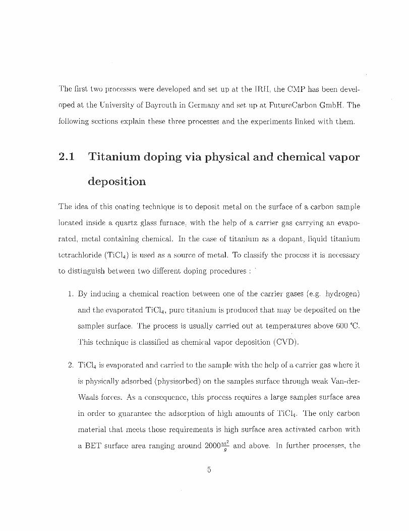
2.1 Titanium doping via physical and chemical vapor
deposition
The idea of this coating technique is to deposit metal on t he surface of a carbon sample
located inside a quartz glass fumace, with the help of a carrier gas carrying an evapo-
rated, met al containing chemical. In the case of t itanium as a dopant , liquid t itanium
tetrachloride (TiCI4 ) is used as a source of metal. To classify the process it is necessary
to distinguish between two different doping procedures :
1. By inducing a chemical reaction between one of the carrier gases (e.g. hydrogen)
and the evaporated TiC14 , pure t itanium is produced that may be deposited on the
samples surface. The pro cess is usually carried out at temperatures above 600 oC .
This technique is classified as chemical vapor deposit ion (CVD).
2. TiCl4 is evaporated and carried to the sample with the help of a carrier gas where it
is physically adsorbed (physisorbed) on t he samples surface through weak Van-der-
Waals forces . As a consequence, this process requires a large samples surface area
in order to guarantee the adsorpt ion of high amounts of TiCI4 . The only carbon
material that meets those requirements is high surface area activated carbon with
a BET surface area ranging around 2000 m2 and above. In further pro cesses , the 9
5
adsorbed TiCl4 can be chemically treated in order to release the t itanium and to
get rid of the chloride. This technique is classified as physical vapor deposition
(PVD) .
For the following set of experiments the super activated carbon type IRH40 was used
which is a in-house product of the IRH and, due to its high surface area, is suitable for
this coating process. The activated carbon IRH40 has a BET-surface area of 2300m2 and 9
a density of 0, 39~ .
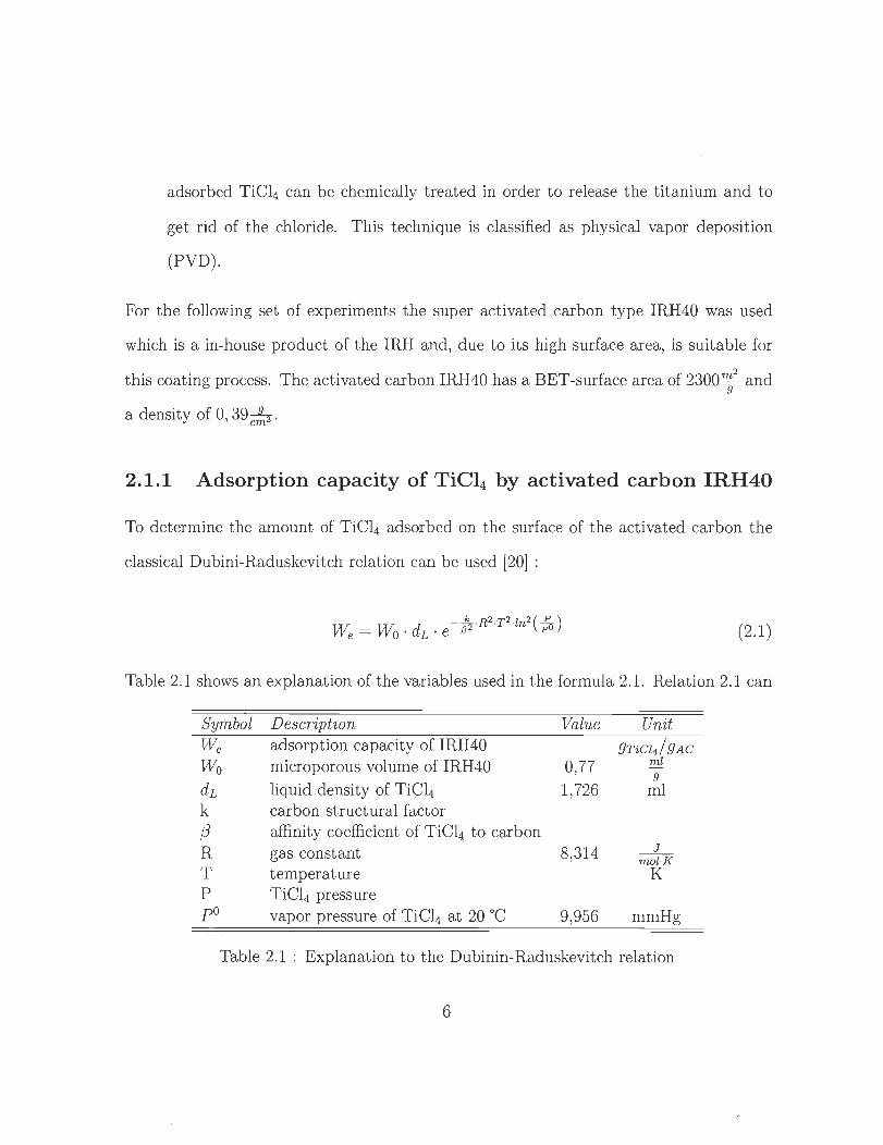
2.1.1 Adsorption capacity of TiCl4 by activated carbon IRH40
To determine the amount of TiCl4 adsorbed on the surface of the activated carbon the
classical Dubini-Raduskevitch relation can be used [20] :
(2 .1 )
Table 2.1 shows an explanation of the variables used in the formula 2.1. Relation 2.1 can
Symbol Description Value Unit We adsorption capacity of IRH40 9 TiCI4!9AC
Wo microporous volume of IRH40 0,77 ml 9
dL liquid density of TiCl4 1,726 ml k carbon structural factor f3 affinity coefficient of TiCl4 to carbon R gas constant 8,314 J
mol·K T temperature K P Ti Cl4 pressure pO vapor pressure of TiCl4 at 20 oC 9,956 mmHg
Table 2.1 : Explanation to the Dubinin-Raduskevitch relation
6
be replaced by the following equation [21] :
(2.2)
where B represents a relative carbon structural constant and Pe t he molecular polariz
ability, which is determined with the refractive index nD (Lorentz formula) :
(n1-1 ) Mw
Pe = n'b + 2 . dL = 38, 10 (2.3)
where nD is the refractive index of TiCL4 (1 ,61) and Mw its molecular weight (189, 68g).
The relative structural constant of IRH40 is determined using equation 2.3 and the
adsorption data of N2 at 77 K. The molecular polarizability of liquid N2 is 4,54 (nD =
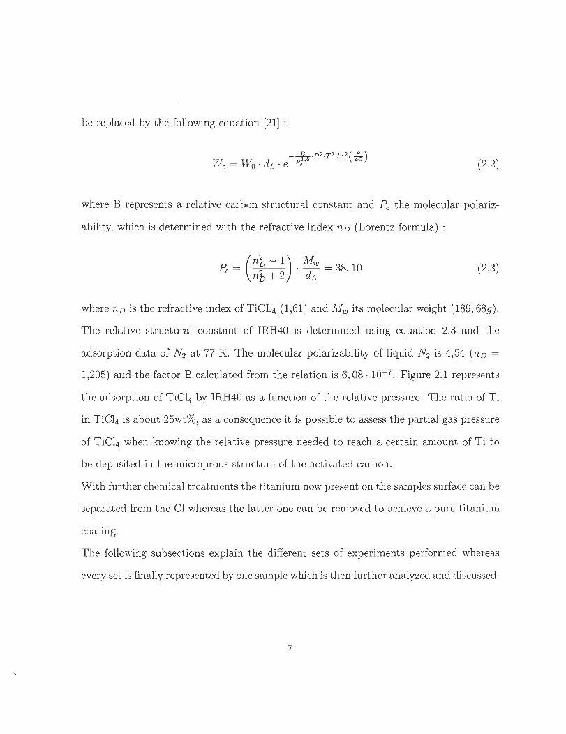
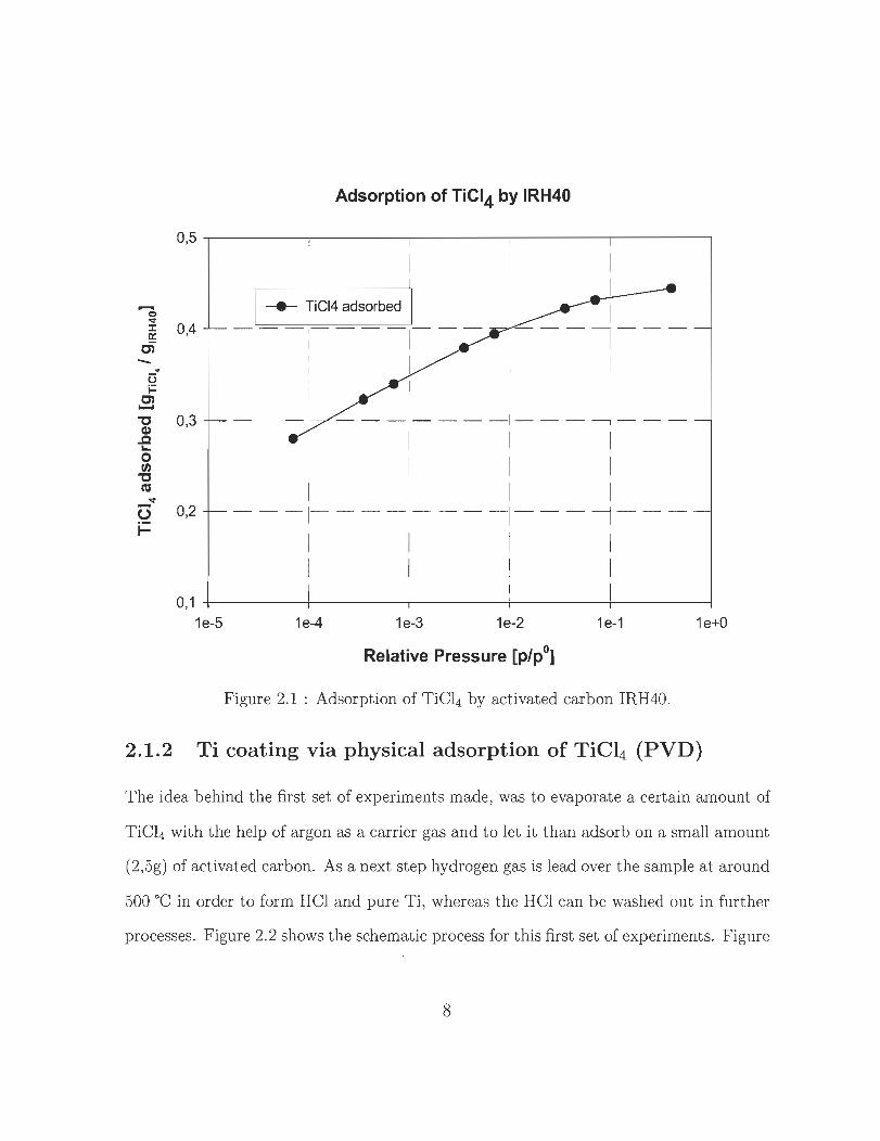
1,205) and the factor B calculated from the relation is 6, 08· 10- 7 . Figure 2.1 represents
the adsorption of TiCl4 by IRH40 as a function of the relative pressure. The ratio of Ti
in TiCl4 is about 25wt%, as a consequence it is possible to assess the partial gas pressure
of TiCl4 when knowing the relative pressure needed to reach a certain amount of Ti to
be deposited in the microprous structure of the activated carbon.
With further chemical treatments the titanium now present on the samples surface can be
separated from the Cl whereas t he latter one can be removed to achieve a pure titanium
coating.
The following subsections explain the different sets of experiments performed whereas
every set is finally represented by one sample which is then further analyzed and discussed.
7
Adsorption of TiCI4 by IRH40
0,5~--------~--------.---------~--------~--------.
...... o
""" ~ 0,4 r;jj -
"C 0,3 Go)
oC 1...
o 1/)
"C n:s -""" U 0,2 i=
__ TiCI4 adsorbed
1
1
1 ----1---
1
1 1
---I----i--- ~---1 1
1 1
1 1
- - -i- - - - 1- - - - 1- - -! - --1 1
1 1
0,1 +---------+-------~~------~--------_+--------~
1e-5 1e-4 1e-3 1e-2 1e-1 1e+0
Relative Pressure [p/po]
Figure 2.1 : Adsorption of TiCl4 by activated carbon IRH40.
2.1.2 Ti coating via physical adsorption of TiCl4 (PVD)
The idea behind the first set of experiments made, was to evaporate a certain amount of
TiCl4 with the help of argon as a carrier gas and to let it than adsorb on a small amount
(2,5g) of activated carbon. As a next step hydrogen gas is lead over the sample at around
500 oC in order to form HCl and pure Ti, whereas the HCl can be washed out in further
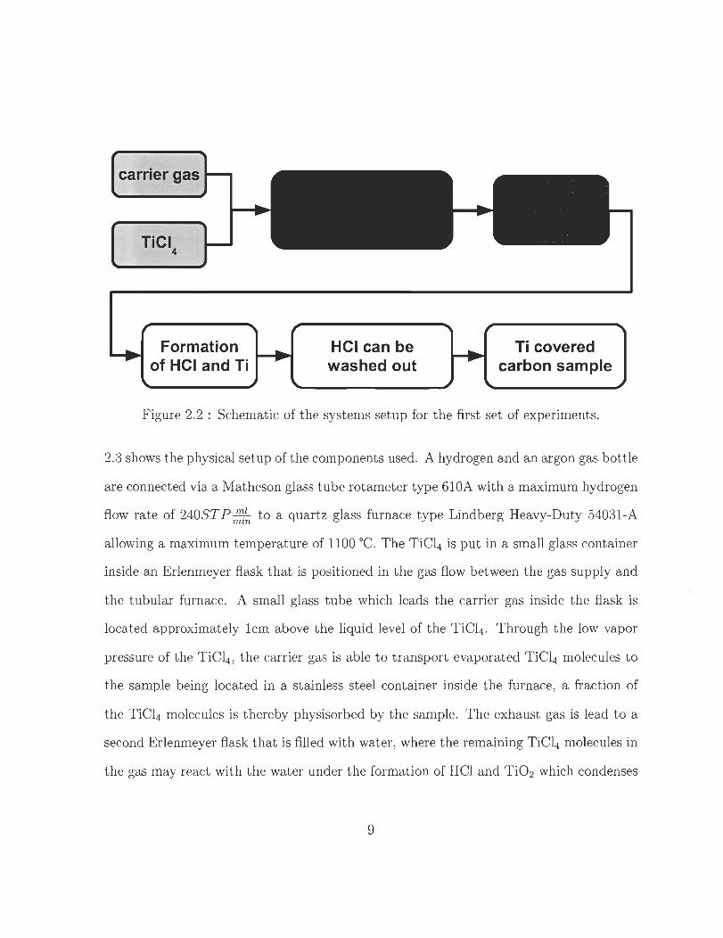
processes. Figure 2.2 shows the schematic process for t his first set of experiments. Figure
8
carrier gas
Formation of HCI and Ti
HCI can be washed out
Ti covered carbon sam pie
Figure 2.2 : Schematic of the systems setup for the first set of experiments .
2.3 shows the physical setup of the components used. A hydrogen and an argon gas bottle
are connected via a Matheson glass tube rotameter type 6l0A with a maximum hydrogen
fiow rate of 240ST P r:~ to a quartz glass fumace type Lindberg Heavy-Duty 5403l-A
allowing a maximum temperature of 1100 oC. The TiCl4 is put in a small glass container
inside an Erlenmeyer fiask that is positioned in the gas fiow between the gas supply and
the tubular fumace. A small glass tube which leads the carrier gas inside the fiask is
located approximately l cm above the liquid level of the TiCl4 . Through the low vapor
pressure of the TiCl4 , t he carrier gas is able to transport evaporated TiCl4 molecules to
the sample being located in a stainless steel container inside the fumace, a fraction of
the TiCl4 molecules is thereby physisorbed by t he sample. The exhaust gas is lead to a
second Erlenmeyer fiask that is filled with water , where the remaining TiCl4 molecules in
the gas may react wit h the water under t he formation of HCl and Ti02 which condenses
9
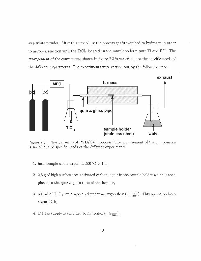
as a white powder. After this procedure the process gas is switched to hydrogen in order
to induce a reaction with the TiC14 located on the sample to form pure Ti and HCL The
arrangement of the components shown in figure 2.3 is varied due to the specifie needs of
the different experiments. The experiments were carried out by the following steps :
furnace
sam pie holder (stainless steel)
exhaust
water
Figure 2.3 : Physical setup of PVDj CVD process. The arrangement of the components is varied due to specifie needs of the different experiments.
1. heat sample under argon at 500 oC > 4 h,
2. 2,5 g of high surface area activated carbon is put in the sample holder which is then
placed in the quartz glass tube of the furnace,
3. 600 /11 of TiC14 are evaporated under an argon fiow (0, 1mZ
in ). This operation lasts
about 12 h,
4. the gas supply is switched to hydrogen (O,5 m1in ),
10
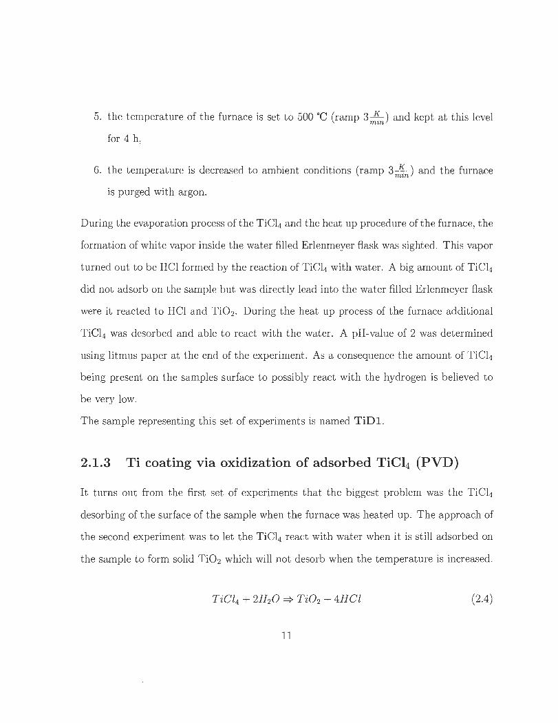
5. the temperature of the fumace is set to 500 oC (ramp 3.K..) and kept at this level mtn
for 4 h,
6. the temperature is decreased to ambient conditions (ramp 3.K..) and the fumace mtn
is purged with argon.
During the evaporation pro cess of the TiCl4 and the heat up procedure of the fumace, the
formation of white vapor inside the water filled Erlenmeyer fiask was sighted. This vapor
tumed out to be HCl formed by the reaction of TiCl4 with water. A big amount of TiCl4
did not adsorb on the sample but was directly lead into the water filled Erlenmeyer fiask
were it reacted to HCl and Ti02 . During the heat up pro cess of the fumace additional
TiCl4 was desorbed and able to react with the water. A pH-value of 2 was determined
using litmus paper at the end of the experiment. As a consequence the amount of TiCl4
being present on the samples surface to possibly react with the hydrogen is believed to
be very low.
The sample representing this set of experiments is named TiD1.
2.1.3 Ti coating via oxidization of adsorbed TiC14 (PVD)
It tums out from the first set of experiments that the biggest problem was the TiCl4
desorbing of the surface of the sample when the fumace was heated up. The approach of
the second experiment was to let the TiCl4 react with water when it is still adsorbed on
the sample to form solid T i0 2 which will not desorb when the temperature is increased.
(2.4)
11
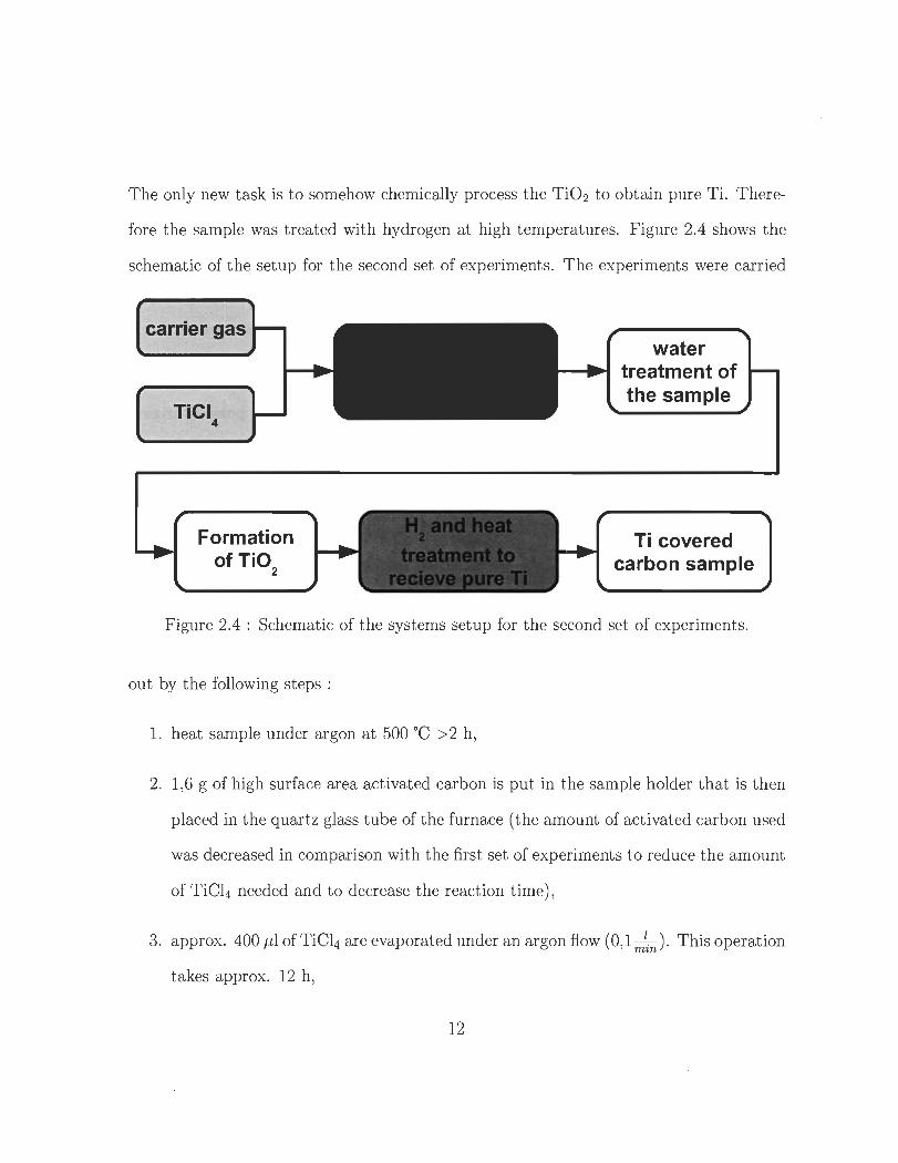
The only new task is to somehow chemically pro cess the Ti02 to obtain pure Ti. There
fore the sample was treated with hydrogen at high temperatures. Figure 2.4 shows the
schematic of the setup for the second set of experiments . The experiments were carried
carrier gas
Formation of Ti0
2
water treatment of the sample
Ti covered carbon sample
Figure 2.4 : Schematic of the systems setup for the second set of experiments.
out by the following steps :
1. heat sample under argon at 500 oC > 2 h,
2. 1,6 g of high surface area activated carbon is put in the sample holder that is then
placed in the quartz glass tube of the furnace (the amount of activated carbon used
was decreased in comparison with the first set of experiments to reduce the amount
of Ti Cl4 needed and to decrease the reaction t ime),
3. approx. 400 j.û of TiCl4 are evaporated under an argon flow ( O , l m~n) . This operation
takes approx. 12 h ,
12
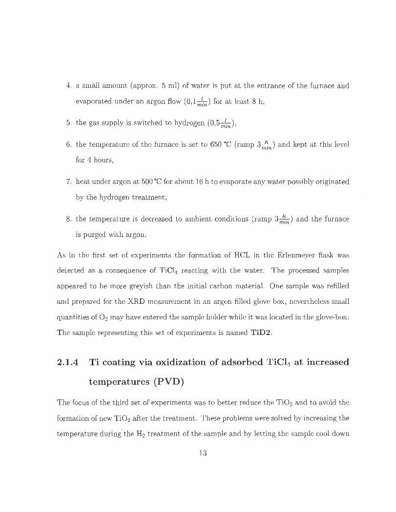
4. a small amount (approx. 5 ml) of water is put at the entrance of the furnace and
evaporated under an argon flow (0,1 m1in) for at least 8 h,
5. the gas supply is switched to hydrogen (0,5rr:in)'
6. the temperature of the furnace is set to 650 oC (ramp 3~n) and kept at this level
for 4 hours,
7. heat under argon at 500 oC for about 16 h to evaporate any water possibly originated
by the hydrogen treatment,
8. the temperature is decreased to ambient conditions (ramp 3.1L) and the furnace mtn
is purged with argon.
As in the first set of experiments the formation of H CL in the Erlenmeyer flask was
detected as a consequence of TiCl4 reacting with the water. The processed samples
appeared to be more greyish than the initial carbon material. One sample was refilled
and prepared for the XRD measurement in an argon filled glove box, nevertheless small
quantities of O2 may have entered the sample holder while it was located in the glove-box.
The sample representing this set of experiments is named TiD2.
2.1.4 Ti coating via oxidization of adsorbed TiC14 at increased
temperatures (PVD)
The focus of the third set of experiments was to better reduce the Ti02 and to avoid the
formation of new Ti02 after the treatment. These problems were solved by increasing the
temperature during the H2 treatment of the sample and by letting the sample cool down
13
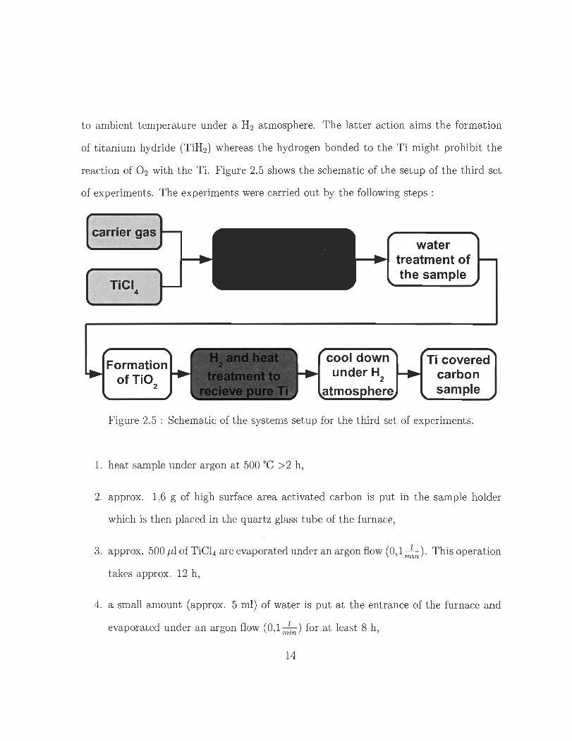
to ambient temperature under a H2 atmosphere. The latter action ai ms the formation
of titanium hydride (TiH2 ) whereas the hydrogen bonded to the Ti might prohibit the
reaction of O2 with the Ti. Figure 2.5 shows the schematic of the setup of the third set
of experiments. The experiments were carried out by the following steps :
Formation of Ti0
2
cool down under H
2
water treatment of the sample
Ti covered carbon sample
Figure 2.5 : Schematic of the systems setup for the third set of experiments.
1. heat sample under argon at 500 oC > 2 h,
2. approx. 1,6 g of high surface area activated carbon is put in the sample holder
which is then placed in the quartz glass tube of the fumace,
3. approx. 500 p'! of TiCl4 are evaporated under an argon flow (0,1-1-. ). This operation mzn
takes approx. 12 h,
4. a small amount (approx. 5 ml) of water is put at the entrance of the fumace and
evaporated under an argon flow (O,lmlin) for at least 8 h,
14
5. heat treatment under argon at 500 oC for about 3 h to evaporate any possibly
condensed water ,
6. the gas supply is switched to hydrogen (0 ,5rr:in) '
7. the temperature of the fumace is set to 800 oC (ramp 3...K..) and kept at t his level mtn
for 4 hours,
8. the temperature is decreased to ambient conditions (ramp 3r!n)' the hydrogen fiow
is kept .
The sample represent ing this set of experiments is named TiD3.
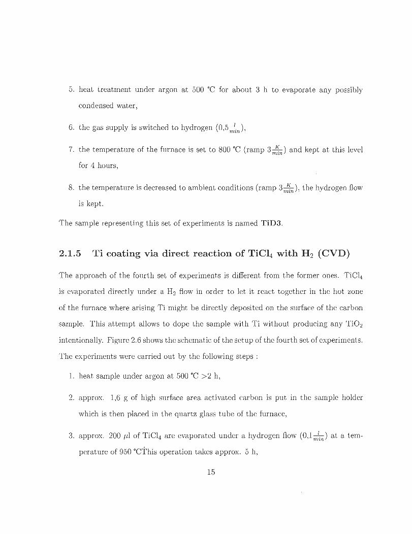
2.1.5 Ti coating via direct reaction of TiCl4 with H 2 (CVD)
The approach of the fourth set of experiments is different from the former ones. TiCl4
is evaporated directly under a H2 fiow in order to let it react together in the hot zone
of t he fumace where arising Ti might be directly deposited on t he surface of the carbon
sample. This at tempt allows to dope the sample with T i without producing any Ti02
intent ionally. Figure 2.6 shows the schemat ic of the setup of the fourth set of experiments .
The experiments were carried out by the following st eps :
1. heat sample under argon at 500 oC > 2 h,
2. approx. 1,6 g of high surface area activated carbon is put in the sample holder
which is then placed in the quartz glass tube of the fumace,
3. approx. 200 ,11 of TiCl4 are evaporated under a hydrogen fiow (O,lrr:in) at a tem
perature of 950 °CThis operation takes approx. 5 h,
15
carrier gas (H
2)
liquid TiCI4
cool down unde ~------------~~ ~------------~~ H
2 atmosphere
Ti covered carbon sample
Figure 2.6 : Schematic of the systems setup for the fourth set of experiments.
4. the temperature is decreased to ambient condit ions (ramp 3~n) ' the hydrogen is
kept flowing.
The sample representing this set of experiments is named TiD4.
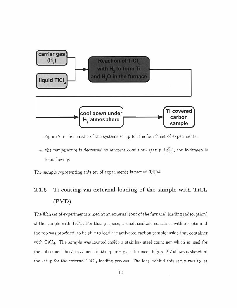
2.1.6 Ti coating via external loading of the sample with TiCl4
(PVD)
The fifth set of experiments aimed at an externa:l (out of the furnace) loading (adsorption)
of the sample with TiCl4 . For that purpose, a small sealable container with a septum at
the top was provided, to be able to load the activated carbon sample inside that container
with TiCl4 . The sample was located inside a stainless steel container which is used for
the subsequent heat treatment in the quartz glass furnace. Figure 2.7 shows a sketch of
the setup for the external TiCl4 loading process. The ide a behind this setup was to let
16
sealable conatiner
stainless steel container containing -f---f~ the carbon sample
septum
liquid TiCI4 ----I---J:.-~+-J::=i;:-
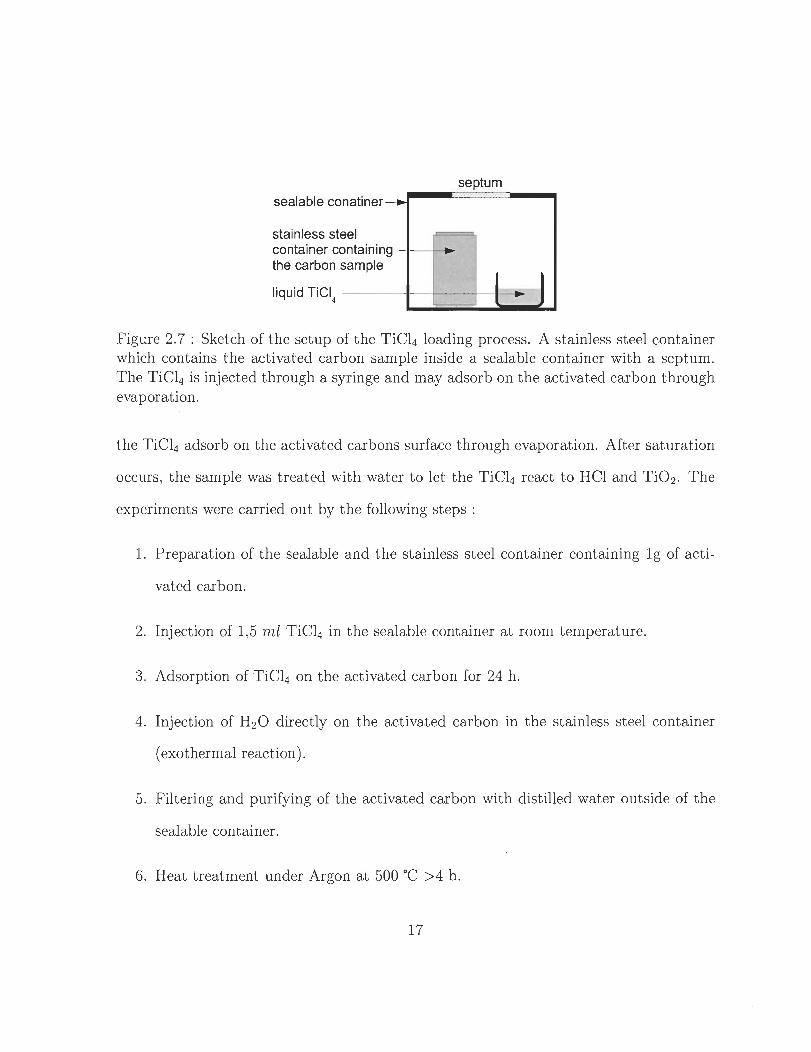
Figure 2.7 : Sketch of the setup of t he TiCl4 loading process. A stainless steel container which contains the activated carbon sample inside a sealable container with a septum. The TiCl4 is injected through a syringe and may adsorb on the activated carbon through evaporation.
the TiCl4 adsorb on the activated carbons surface t hrough evaporation. After saturation
occurs, the sample was t reated with water to let t he TiCl4 react to HCl and TiÜ2' The
experiments were carried out by t he following steps :
1. Preparation of the sealable and the stainless steel container containing 19 of acti-
vated carbon.
2. Injection of 1,5 ml TiC14 in the sealable container at room temperature.
3. Adsorption of TiCl4 on the activated carbon for 24 h.
4. Injection of H2ü directly on the activated carbon in the stainless steel container
(exothermal reaction).
5. Filtering and purifying of the activated carbon with distilled water outside of the
sealable container.
6. Heat t reatment under Argon at 500 oC > 4 h.
17
7. Reduction of the Ti02 to pure Ti through H 2 treatment at 950 oC >4 h (This step
was repeated 3 times).
The sample representing this set of experiments is named TiD5.
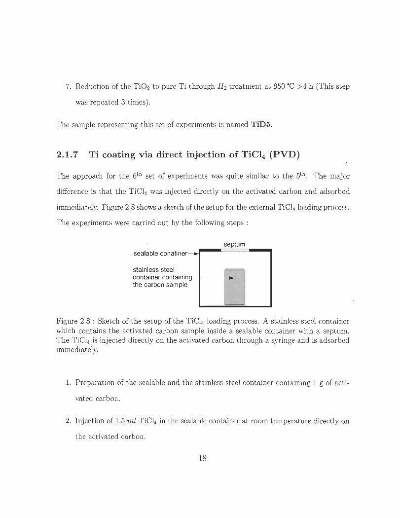
2.1.7 Ti coating via direct injection of TiC14 (PVD)
The approach for the . 6th set of experiments was quite similar to the 5th . The major
difference is that the TiCl4 was injected directly on the activated carbon and adsorbed
immediately. Figure 2.8 shows a sketch of the setup for the external TiCl4 loading process.
The experiments were carried out by the following steps :
septum sealable conatiner
stainless steel container containing -1--
the carbon sam pie
Figure 2.8 : Sketch of the setup of the TiCl4 loading process. A stainless steel container which contains the activated carbon sample inside a sealable container with a septum. The TiCl4 is injected directly on the activated carbon through a syringe and is adsorbed immediately.
1. Preparation of the sealable and the stainless steel container containing 1 g of acti-
vated carbon.
2. Injection of 1,5 ml TiCl4 in the sealable container at room temperature directly on
the activated carbon.
18
3. Adsorpt ion of TiC14 on the activated carbon for 1h.
4. Injection of H2 0 directly on the activated carbon in the stainless steel container
(exothermal reaction).
5. Filtering and purifying of the activated carbon with distilled water outside of the
sealable container.
6. Heat treatment under Argon at 500 oC >4 h.
7. Reduction of the Ti02 to pure Ti through H 2 treatment at 950 oC >4 h (This step
was repeated 3 t imes) .
The sam pIe represent ing this set of experiments is named TiD6.
19
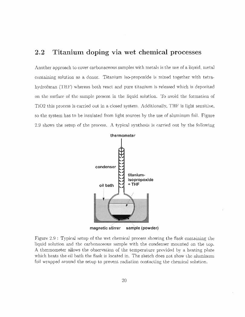
2.2 Titanium doping via wet chemical pro cesses
Another approach to cover carbonaceous samples with metals is the use of a liquid, metal
containing solut ion as a donor. Titanium iso-propoxide is mixed together with tetra
hydrofuran (THF) whereas both react and pure t itanium is released which is deposited
on the surface of the sample present in the liquid solution. To avoid the formation of
Ti02 this pro cess is carried out in a closed system. Addit ionally, THF is light sensit ive,
so the system has to be insulated from light sources by the use of aluminum foil. Figure
2.9 shows the setup of t he process. A typical synthesis is carried out by the following
thermometer
condenser
titaniumisopropoxide
oil bath + THF
magnetic stirrer sam pie (powder)
Figure 2.9 : Typical setup of the wet chemical process showing the flask containing the liquid solut ion and the carbonaceous sample with the condenser mounted on the top. A thermometer allows the observation of the temperature provided by a heating plate which heats the oil bath the flask is located in. The sketch does not show the aluminum foil wrapped around t he setup to prevent radiation contacting the chemical solut ion.
20
steps :
1. 25 ml titanium iso-propoxide and 100 ml THF is put in a 5 liter fiask together with
about 1,5 g of a carbonaceous powdered sample.
2. A magne tic stirrer is put in the fiask.
3. A condenser with a temperature sensor on the top is mounted on top of the fiask
and the system is hermetically sealed with sealing agent .
4. The bottom of the glass fiask is put in an oil bath on top of the heating plate. To
avoid chemical reactions caused by incidence of light , the system is also optically
insulated by aluminum foil.
5. The temperature of the heating plate is set to about 80 oC and the magnetic stirrer
is activated.
6. The system remains in t hat state for 3 days.
7. The pro cess is finished, the sample can be refilled and prepared for the heat treat
ment in a glove box to avoid contamination. with O2.
2.2.1 Amount of chemicals used
19 carbon sample equals 112 mol carbon atoms. For a sufficient t itanium surface coverage
an amount of 1 titanium atom for 3 carbon atoms seems to be adequate. The amount
of t itanium iso-propoxide necessary for 19 carbon sample can be calculated from its
molecular weight (See table 2.2)
21
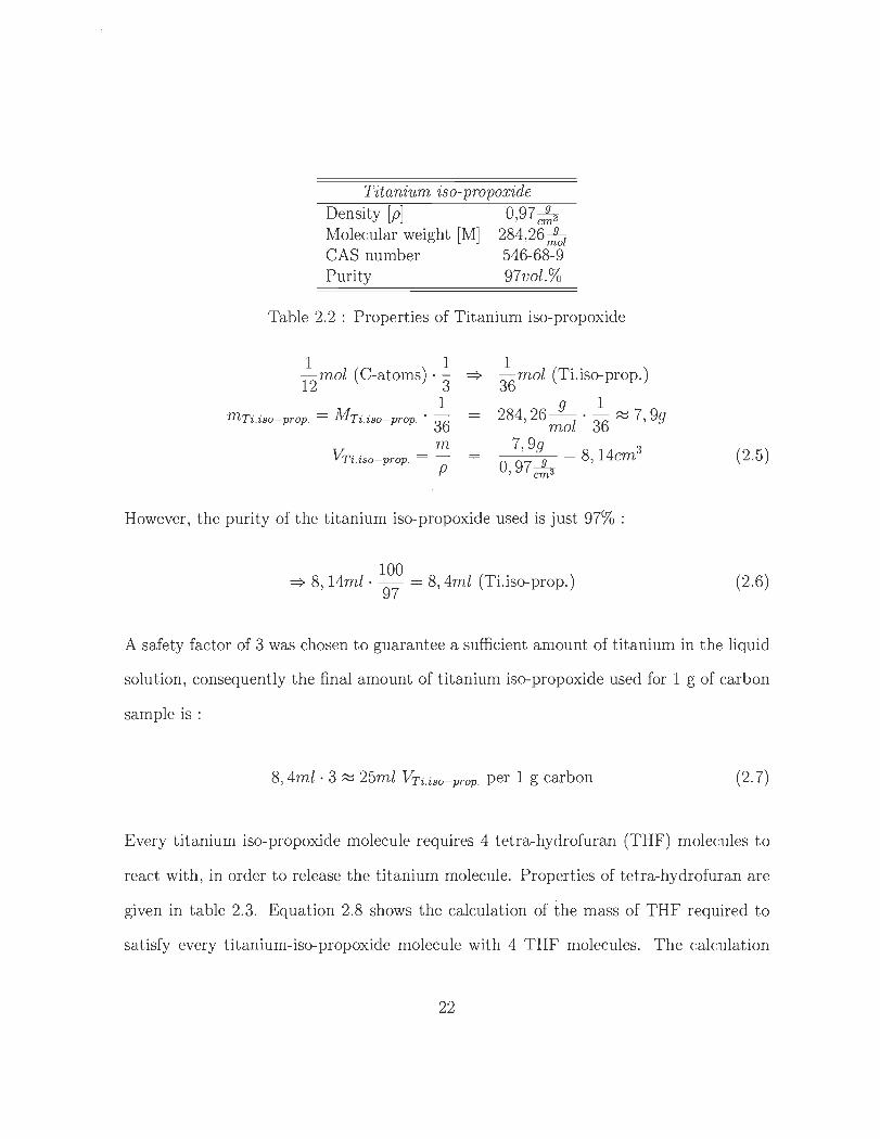
Titanium iso-propoxide Density [pl 0 ,97~ Molecular weight [M] 284 ,26~ CAS number 546-68-9 Purity 97vol. %
Table 2.2 : Propert ies of Titanium iso-propoxide
1 1 12 mol (C-atoms) . "3
1 mTi.iso-prop. = MTi.iso-prop . . 36
m VTi.iso-prop. = -
p
1 =} 36 mol (Ti.iso-prop.)
9 1 284, 26 mol ' 36 ~ 7, 99
7, 99 = 8 14 3 o 97 ---.IL ,cm , C1n3
However, the purity of the titanium iso-propoxide used is just 97% :
=} 8, 14ml . 19°7° = 8, 4ml (Ti.iso-prop.)
(2.5)
(2 .6)
A safety factor of 3 was chosen to guarantee a sufficient amount of t itanium in the liquid
solut ion, consequently the final amount of t itanium iso-propoxide used for 1 g of carbon
sample is :
8,4ml . 3 ~ 25ml VTi.iso-prop. per 1 g carbon (2.7)
Every t itanium iso-propoxide molecule requires 4 tetra-hydrofuran (THF) molecules to
react with, in order to release the titanium molecule. Properties of tetra-hydrofuran are
given in table 2.3. Equation 2.8 shows the calculation of the mass of THF required to
satisfy every titanium-iso-propoxide mole cule with 4 THF molecules. The calculation
22
includes a safety factor of 2.
M Ti . iso-prop. 284 , 26g
MTHF 72 , llg
MTHF,required 4·2 · 72, l1g = 576, 88g ~ 2 . ]V!ri.iso-prop.
=} mTHF,required ~ 2· mTi.iso-prop. (2.8)
According to the different densities of both substances, the volume of THF required is
calculated by :
m P v
mT H F,required ~ 2 · mTi.iso-prop.
V T H F,required 2 · PTHF . VTi.iso-prop.
PTi .iso-prop.
V T H F,required 2 · 0,889~· 25ml l
cm ~ 46m 0 , 97~
Figure 2.10 shows a model of a tetra-hydrofuran molecule.
tetm-hydrofumn Density [pl 0 ,889~ Molecular weight [M] 72 ,11~
CAS number 109-99-9
Table 2.3 : Properties of tetra-hydrofuran
23
(2.9)
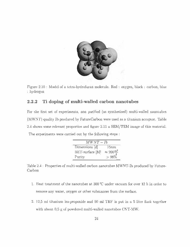
Figure 2. 10 : Model of a tetra-hydrofuran molecule. Red: oxygen, black : carbon, blue : hydrogen
2.2.2 Ti doping of multi-walled carbon nanotubes
For the first set of experiments, non purified (as synthesized) multi-walled nanotubes
(MWNT ) quality lb produced by FutureCarbon were used as a titanium acceptor. Table
2.4 shows sorne relevant properties and figure 2.11 a SEM/ TEM image of this material.
The experiments were carried out by the following steps :
MWNT -Ib Dimensions [dl BET-surface [M] Purity
15nm ~ 200 m 2
9 > 98%
Table 2.4 : Propert ies of multi-walled carbon nanotubes MWNT-lb produced by FutureCarbon
1. Heat treatment of the nanotubes at 300 oC under vacuum for over 12 h in order to
remove any water , oxygen or ot her subst ances from the surface.
2. 12,5 ml t itanium iso-propoxide and 90 ml THF is put in a 5 liter fiask together
with about 0,5 g of powdered mult i-walled nanotubes CNT-MW.
24
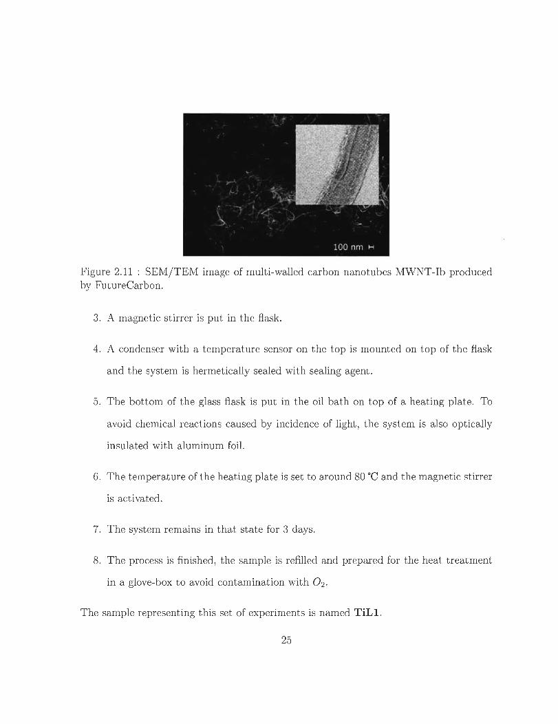
Figure 2.11 : SEM/TEM image of multi-walled carbon nanotubes MWNT-Ib produced by FutureCarbon.
3. A magnetic stirrer is put in the flask.
4. A condenser with a temperature sensor on the top is mounted on top of the flask
and the system is hermetically sealed with sealing agent.
5. The bottom of the glass flask is put in the oil bath on top of a heating plate. To
avoid chemical reactions caused by incidence of light, the system is also optically
insulated with aluminum foil.
6. The temperature of the heating plate is set to around 80 oC and the magnetic stirrer
is activated.
7. The system remains in that state for 3 days.
8. The process is finished, the sample is refilled and prepared for the heat treatment
in a glove-box to avoid contamination with O2 .
The sample representing this set of experiments is named TiLl.
25
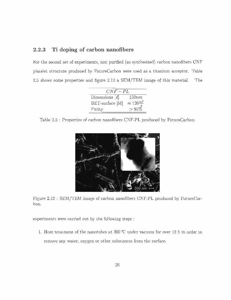
2.2.3 Ti doping of carbon nanofibers
For the second set of experiments, non purified (as synthesized) carbon nanofibers CNF
platelet structure produced by FutureCarbon were used as a t itanium acceptoI. Table
2.5 shows sorne properties and figure 2.12 a SEM/TEM image of this material. The
CNF-PL Dimensions [dl BET-surface [M] Purity
150nm
~ 120 m2
9
> 95%
Table 2.5 : Properties of carbon nanofibers CNF-PL produced by FutureCarbon.
Figure 2.12 : SEM/TEM image of carbon nanofibers CNF-PL produced by FutureCarbon.
experiments were carried out by the following steps :
1. Heat treatment of the nanotubes at 300 oC under vacuum for over 12 h in order to
remove any water, oxygen or other substances from the surface.
26
2. 17 ml titanium iso-propoxide and 38 ml THF is put in a 5 liter fiask together wit h
about 1 g of powdered nanofibers CNF-PL.
3. A magnetic stirrer and boiling stones are put in the fiask.
4. A condenser with a temperature sensor on the t op is mounted on top of the fiask
and the system is hermetically sealed.
5. The bot tom of the glass fiask is put in the oil bath on top of t he heating plate . To
avoid chemical reactions caused by incidence of light , the system is also optically
insulated with aluminum foil.
6. The temperature of the heating plate is set at about 80 oC and the magnetic stirrer
is activated.
7. The system remains in that state for 3 days.
8. The process is finished, the sample is refilled and prepared for the heat t reatment
in a glove box to avoid contamination with O2
The sample represent ing this set of experiments is named TiL2.
2.2.4 Ti doping of high surface area activated carbon
For the t hird set of experiments , activated carbon type IRH40 produced from the Institut
de Recherche sur l'Hydrogène (IRH) was used as a t itanium acceptoI. The experiments
were carried out by the following steps :
27
1. Heat treatment of the activated carbon at 300 oC under vacuum for over 12 h in
order to remove any water, oxygen or other substances from the surface.
2. 26 ml titanium iso-propoxide and 155 ml THF is put in a 5 liter flask together with
about 1,46 g of powdered IRH40.
3. A magne tic stirrer and boiling stones are put in the flask.
4. A condenser with a temperature sensor is mounted on top of the flask. The system
is hermetically sealed.
5. The bottom of the glass flask is put in the oil bath on top of the heating plate. To
avoid chemical reactions caused by incidence of light, the system is also optically
insulated with aluminum foil.
6. The temperature of the heating plate is set at about 80 oC and the magnetic stirrer
is activated.
7. The system remains in that state for 3 days.
8. The pro cess is finished; the sample is refilled and prepared for the heat treatment
in a glove box to avoid contamination with O2 .
The sam pIe representing this set of experiments is named TiL3.
28
2.3 Palladiumjplatinum doping via Colloidal Micro
wave Processing (CMP)
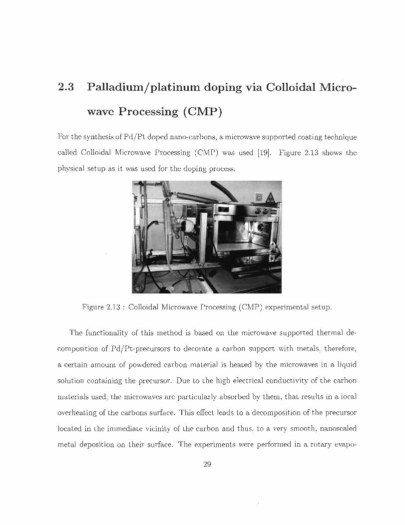
For the synthesis of Pd/Pt doped nano-carbons, a microwave supported coating technique
called Colloidal Microwave Processing (CMP) was used [19J. Figure 2.13 shows the
physical setup as it was used for the doping process.
Figure 2.13 : Colloidal Microwave Processing (CMP) experimental setup.
The functionality of this method is based on the microwave supported thermal de
composition of Pd/Pt-precursors to decorate a carbon support with metals , therefore,
a certain amount of powdered carbon material is heated by the microwaves in a liquid
solution containing the precursor. Due to the high electrical conductivity of the carbon
materials used, the microwaves are particularly absorbed by them, that results in a local
overheating of the carbons surface. This effect leads to a decomposition of the precursor
located in the immediate vicinity of the carbon and thus, to a very smooth, nanoscaled
metal deposition on their surface. The experiments were performed in a rotary evapo-
29
rator , equipped with a 2,lkW commercial microwave oven, operating at a frequency of
2,45GHz, the precursors used were platinum 2,4-pentanedione (Pt(C5H70 2)2) and palla
dium 2,4-pentanedione (Pd( C5H 70 2h). Experiments were carried out at FutureCarbon
GmbH with CNT-MW (purified), CNF-PL (purified) as well as high surface area acti
vated carbon IRH40 as a carbon support. The metal content on the samples was adjusted
by the mass of precursor used during the synthesis, for all samples the aim was to gain
a metal density of 8wt%. The samples obtained are identified as IRH40 (8wt% Pd) ,
CNT-MW (8wt% Pd) , CNF-PL (8wt% Pd) and CNF-PL (8wt% Pt).
30
Chapter 3
Sample Characterization
3.1 Solid state analytics
3.1.1 X -ray crystallography (XRD)
X-ray diffraction is an analysis technique commonly used in materials science for the
characterization ofthe crystalline structure of a solid material [22 , 23]. The physical basis
of this method is the diffraction of X-rays of a certain energy on the spatial periodical
arranged lattice planes in the solid material that are representative for a certain crystalline
structure. Diffraction occurs wh en the distance of the lattice planes is in the range of
the wavelength of the X-rays, which usually is in the dimension of about lOOpm. In the
electro-magnetic field of t he incoming X-rays of a certain wavelength, the electrons in the
solid material are forced to vibrate, and as a consequence, do emit X-rays themselves wit h
the same wavelength. These re-emitted X-rays now interfere constructive and destructive
depending on the crystalline structure of the atoms of t he solid. By observing the solid
at different angles, constructive and destructive interference can be visualized in a graph
by plotting the viewing angle versus the X-ray intensity recorded at the certain angle.
By the comparison of the spectra gained with the XRD elements database, the sample
can be characterized regarding its chemical compounds and elements. The condition for
constructive interference can be expressed by Bragg's law :
n).. = 2d . sin(8) (3 .1 )
whereas n is an integer, ).. the wavelength of the X-rays, d is the spacing between the
planes in the atomic lattice, and 8 is the angle between the incident ray and the scattering
planes.
In this thesis , X-ray diffraction was used to characterize most of the samples synthesized.
However, goal of the synthesis process always was to generate a monolayer that can not
be detected by XRD, as a consequence peaks appearing in the XRD spectra were an
indicator of thick coating. In comparison with X-ray Photoelectron Spectroscopy (XPS)
described in subsection 3.1.2, XRD is a characterization technique which allows not just
the analysis of the first 10nm of the samples surface, but features an insight through the
whole diameter of the sample.
3.1.2 X-ray Photoelectron Spectroscopy (XPS)
X-ray Photoelectron Spectroscopy (XPS) is a quantitative spectroscopic technique that
allows the analysis of the empirical formula, the chemical state and the electronic state
of the elements that exist on a samples surface. An electron is ejected from a core
32
Ievei by an X-ray photon of the energy hv. The kinetic energy (EK ) and the number
of these emitted photoelectrons that escape from the top 1 to lOnm of the sam pIe is
then anaIyzed by an electron spectrometer [24, 25]. However , the kinetic energy of the
electrons is not an intrinsic material property but is dependent on the photon energy
of the X-rays empIoyed, the binding energy (EB ) is the parameter which ident ifies the
electron specifically, both in terms of its element and atomic level. The relationship
between t he X-ray photon energy, the kinetic energy and the binding energy is :
EB = hv- EK - W (3.2)
were W is the spectrometer work function. All three quant it ies known on the right hand
side of the equation allow the determination of the binding energy.
By count ing the number of electrons being ejected at a certain X-ray energy and plotting
this number of electrons ejected per second versus the binding energy, one receives the
XPS spectra characterizing the surface of the sampie. By comparing this spectra with
the XPS elements dat abase, the samples surface can be characterized and classified. A
few sam pIe were characterized by this method within this thesis.
33
3.2 Hydrogen adsorption measurements
This section deseribes the two methods generally used for the determination of a samples
hydrogen adsorption eapaeity. Both methods deseribed have major advantages and disad
vantages. The volumetrie measurement setups available at the IRH and at FutureCarbon
GmbH complete eaeh other regarding the pressure range in whieh the samples adsorp
tion eapaeity ean be determined. For low pressure eharaeterization « 0, 1 MPa), the
automatie measuring apparatuses at the IRH ean be used (Quantaehrome Autosorb® -1
and Mieromerities® ASAP 2020) , whereas for high pressure measurements up to 4 MPa
the self eonstructed Sieverts apparatus at FutureCarbon GmbH is used. AH volumetrie
setups used, allow the determination of the adsorption eapaeity at temperatures down to
77 K. For measurements at room temperature and pressures up to 4 MPa the gravimetrie
setup at the IRH is used due to its better aeeuraey.
3.2.1 Volumetrie method (Sieverts apparatus)
The basic idea of the volumetrie method is to determine the hydrogen adsorption eapaeity
of a sample via gas expansions from a referenee volume to a measuring volume whereas
the sample is loeated inside the measuring volume. The pressure change between those
expansions allows the ealculation of the amount of gas adsorbed on the sam pIe [26, 27].
The foHowing list explains the setup of sueh a system. Figure 3.1 prints out a typieal
setup for a volumetrie test bed (Sieverts apparatus) and figure 3.2 shows the physieal
setup of sueh a test bed at FutureCarbon GmbH.
34
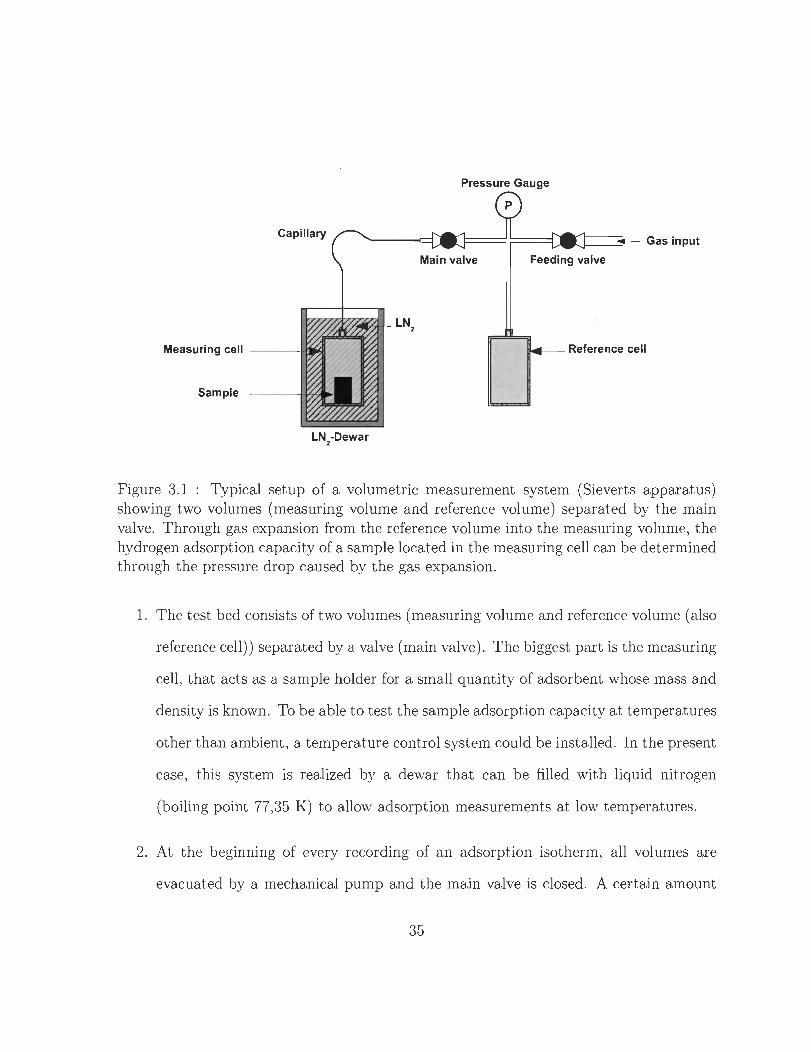
Pressure Gauge
Gas input
Measuring cell ----In!..,. Reference cell
Sample
LN2-Dewar
Figure 3.1 : Typical setup of a volumetrie measurement system (Sieverts apparatus) showing two volumes (measuring volume and reference volume) separated by the main valve. Through gas expansion from t he reference volume into the measuring volume, t he hydrogen adsorpt ion capacity of a sample located in t he measuring cell can be determined through the pressure drop caused by t he gas expansion.
1. The test bed consists of two volumes (measuring volume and reference volume (also
reference ceIl)) separated by a valve (main valve) . The biggest part is the measuring
ceIl, that acts as a sam pIe holder for a small quant ity of adsorbent whose mass and
density is known. To be able to test the sample adsorpt ion capacity at temperatures
other t han ambient, a temperature control system could be installed. In the present
case, t his system is realized by a dewar that can be filled with liquid nitrogen
(boiling point 77,35 K) to allow adsorpt ion measurements at low temperatures.
2. At t he beginning of every recording of an adsorpt ion isotherm, aIl volumes are
evacuated by a mechanical pump and the main valve is closed. A certain amount
35
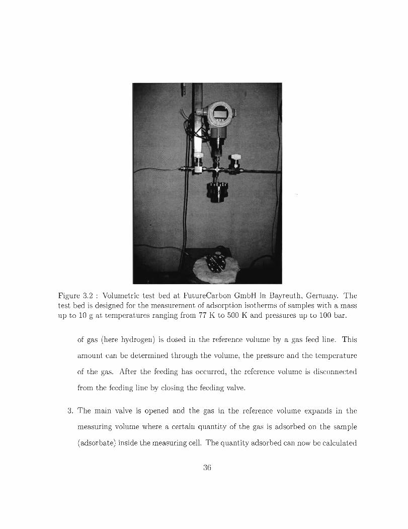
Figure 3.2 : Volumetrie t est bed at FutureCarbon GmbH in Bayreut h, Germany. The test bed is designed for the measurement of adsorpt ion isot herms of samples wit h a mass up to 10 g at temperatures ranging from 77 K to 500 K and pressures up to 100 bar.
of gas (here hydrogen) is dosed in the reference volume by agas feed line. This
amount ean be determined through the volume, the pressure and the temperature
of the gas. After the feeding has oeeurred , the reference volume is diseonnected
from the feeding line by closing the feeding valve.
3. The main valve is opened and the gas in the referenee volume expands in the
measuring volume where a certain quant ity of the gas is adsorbed on the sample
(adsorbate) inside the measuring cell. The quant ity adsorbed ean now be ealculated
36
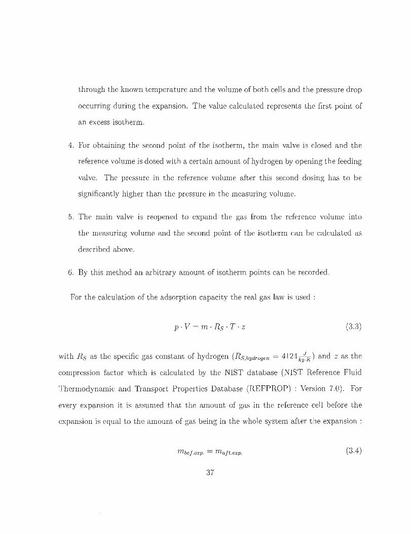
through the known temperature and the volume of both cells and the pressure drop
occurring during the expansion. The value calculated represents the first point of
an excess isotherm.
4. For obtaining the second point of the isotherm, the main valve is closed and the
reference volume is dosed with a certain amount of hydrogen by opening the feeding
valve. The pressure in the reference volume after this second dosing has to be
significantly higher than the pressure in the measuring volume.
5. The main valve is reopened to expand the gas from the reference volume into
the measuring volume and the second point of the isotherm can be calculated as
described above.
6. By this method an arbitrary amount of isotherm points can be recorded.
For the calculation of the adsorption capacity the real gas law is used :
p . V = m . Rs . T . z (3.3)
with Rs as the specific gas constant of hydrogen (Rs,hydrogen = 4124 k/K) and z as the
compression factor which is calculated by the NIST database (NIST Reference Fluid
Thermodynamic and Transport Properties Database (REFPROP) : Version 7.0). For
every expansion it is assumed that the amount of gas in the reference cell before the
expansion is equal to the amount of gas being in the who le system after the expansion:
mbef. exp. = malt.exp. (3.4)
37
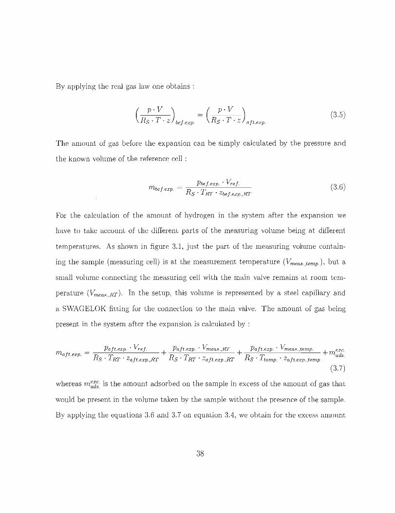
By applying the real gas law one obtains :
( p ·V ) ( p ·V )
Rs . T . Z bef. exp. - Rs' T . Z aft.exp. (3.5)
The amount of gas before the expansion can be simply calculated by the pressure and
the known volume of the reference cell :
Pbef. exp . . Vref. mbef. exp. = - --'-----'----'----
Rs . TRT . Zbef. exp. ,RT (3.6)
For the calculation of the amount of hydrogen in the system after the expansion we
have to take account of the different parts of the measuring volume being atdifferent
temperatures. As shown in figure 3.1, just the part of the measuring volume contain
ing the sample (measuring cell) is at the measurement temperature (Vmeas .,temp.) , but a
small volume connecting the measuring cell with the main valve remains at room tem-
perature (Vmeas., RT). In the setup, this volume is represented by a steel capillary and
a SWAGELOK fitting for the connection to the main valve. The amount of gas being
present in the system after the expansion is calculated by :
_ P aft .exp . . Vref. + Paft.exp. · Vmeas.,RT + Paft .exp. · Vmeas.,temp. + m exc. maft.exp. - R T R T R T, Z ads.
S ' RT ' Zaft .exp. ,RT S ' RT ' Zaft. exp. ,RT S ' temp. · aft .exp.,temp
(3.7)
whereas m~d~: is the amount adsorbed on the sample in excess of the amount of gas that
would be present in the volume taken by the sample without the presence of the sample.
By applying the equations 3.6 and 3.7 on equation 3.4, we obtain for the excess amount
38
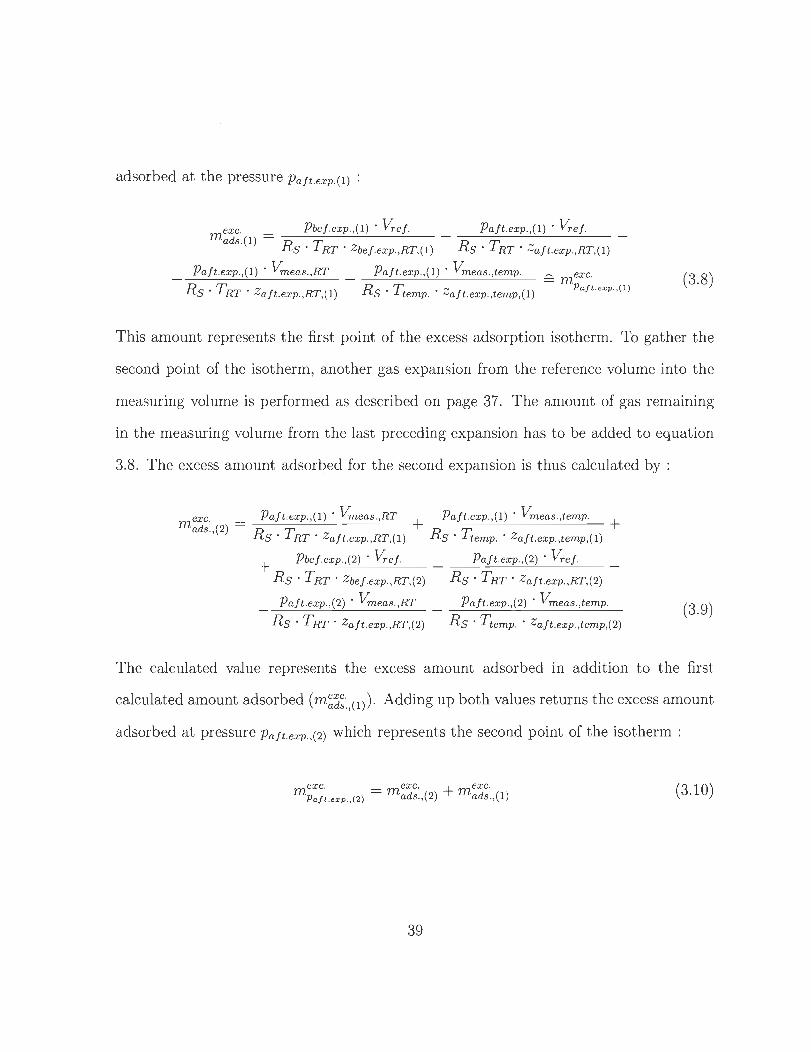
adsorbed at the pressure Paft .exp.(l ) :
Pbef. exp.,( l) . Vref. Paft .exp. ,(l) . Vr ef. exc. mads.(l ) =
Rs . TRT . z bef. exp. ,RT,( l ) Rs . TRT . Zaft.exp. ,RT,( l)
Paft .exp. ,(l ) . Vmeas.,RT Paft. exp.,( l) . Vmeas. ,temp. == m exc.
Rs . TRT . Z f ( ) Rs T, . Z f ( ) Pajt .exp. ,( l ) a t .exp.,RT, 1 . tempo a t.exp. ,temp, 1 (3 .8)
This amount represents the first point of the excess adsorption isotherm. To gather the
second point of the isotherm, another gas expansion from the reference volume into the
measuring volume is performed as described on page 37. The amount of gas remaining
in the measuring volume from the last preceding expansion has to be added to equation
3.8. The excess amount adsorbed for the second expansion is thus calculated by :
m exc. _ ads. ,(2) -
Paft. exp. ,( l ) . Vmeas .,RT + Paft.exp.,( l ) · Vmeas., temp. + Rs . TRT . Zaft. exp. ,RT,( l) Rs . Ttemp . . Za ft .exp. ,temp ,( l)
+ Pbef. exp.,(2) . Vr ef . Paft. exp. ,(2) . Vref.
Rs . T RT . Zbef. exp. ,RT,(2) Rs . T RT . Za ft. exp. ,RT,(2)
Paft.exp. ,(2) . Vmeas.,RT
Rs . TRT . Za ft .exp.,RT,(2)
Paft. exp.,(2) . Vmeas. ,temp.
Rs . Ttemp . . Zaft.exp.,temp,(2) (3.9)
The calculated value represents the excess amount adsorbed in addition to the first
calculated amount adsorbed (m~d~·. , ( l )) ' Adding up both values returns the excess amount
adsorbed at pressure Paft.exp. ,(2) which represents the second point of the isotherm :
m exc. _ m exc. + m exc. P a jt .exp.,(2) - ads.,(2) ads. ,(l ) (3. 10)
39
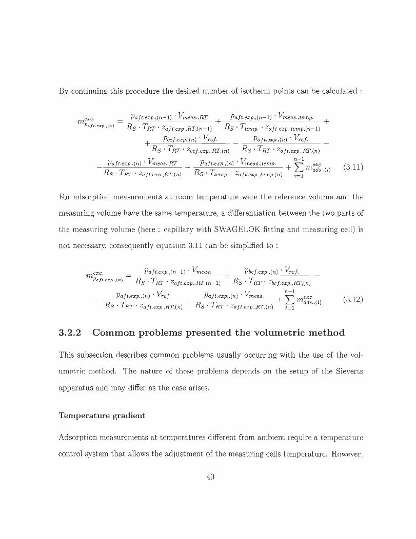
By continuing this procedure the desired number of isotherm points can be calculated :
m exc. Pa f t.exp. ,(n)
Pajt .exp.,(n-l ) . Vmeas. ,RT + Pajt.exp. ,(n-l ) · Vmeas.,temp. + Rs . TRT . Zajt. exp. ,RT,(n-l) Rs . Ttemp . . Zajt. exp.,t emp,(n-l )
+ Pbej.exp. ,(n ) . Vrej. Pajt.exp. ,(n ) . Vr ej.
Rs . TRT . Zbej. exp. ,RT,(n ) Rs . TRT . Zajt. exp.,RT,(n )
Pajt.exp., (n) . Vmeas.,RT
Rs . TRT . Zajt. exp.,RT,(n)
V. n-l Pajt .exp. ,(n ) · m eas.,temp. + '"' exc.
R . 1', . Z L.J mads.,(i ) s tempo ajt.exp. ,temp,(n ) i=l (3.11)
For adsorption measurements at room temperature were the reference volume and the
measuring volume have the same temperature , a differentiation between the two parts of
the measuring volume (here : capillary with SWAGELOK fitting and measuring cell) is
not necessary, consequently equation 3. 11 can be simplified to :
m exc. Paft .exp. ,(n)
Pajt.exp. ,(n-l ) . V m eas. + Pbej.exp.,(n ) . Vrej.
Rs . TRT . Zajt.exp.,RT,(n-l ) Rs . TRT . Zbej. exp.,RT,(n )
P ajt.exp.,(n ) . Vrej. V. n-l
Pajt .exp.,(n ) · m eas. + '"' exc. R . T . Z L.J mads.,(i)
S RT ajt.exp. ,RT,(n ) i=l (3.12)
Rs . TRT . Zajt.exp. ,RT,(n )
3.2.2 Common problems presented the volumetrie method
This subsection describes common problems usually occurring with the use of the vol-
umetric method. The nature of these problems depends on the setup of the Sieverts
apparatus and may differ as the case arises.
Temperature gradient
Adsorption measurements at temperatures different from ambient require a temperature
control system that allows the adjustment of the measuring cells temperature. However,
40
having the measuring ceIl and the reference ceIl at different temperatures leads to a tem
perature gradient somewhere in t he system, which makes it very difficult to calculate the
amount of gas being present in t hat part of the system. This problem can be minimized
by using a connection wit h a very low volume between t he measuring cell and the refer
ence cell. In the present system used, this connection has been realized by a 30 cm steel
capillary with an inside diameter of 0, 15mm. This leads to an internaI volume of about
0,0053 cm3 that is around 4 orders of magnit ude smaller than t he volume orthe rest of
the system. By having t he temperature gradient occur over such a small volume, the
amount of gas being present in t he capillary can be calculated by assuming an averaged
temperature aIl over t he capillary.
Identification of the systems volume
Wh en setting up a volumetrie system from scratch, usuaIly neither the. reference volume
nor the measuring volume is known, however both values are required for t he adsorp
tion measurements . The determination of both values requires the use of a . weIl known
calibration volume Vcal e.g. in form of a sphere or another body with simple geometry,
which can be placed in the measuring volume of the Sieverts apparatus. The volumes
are then determined the following way :
1. The empty system (no sample or calibration volume used) is pumped out by the
use of the mechanical pump.
2. The main valve is closed and the reference volume is dosed wit h a certain amount
of hydrogen gas. The feeding valve is closed after this dosing. The pressure gauge
41
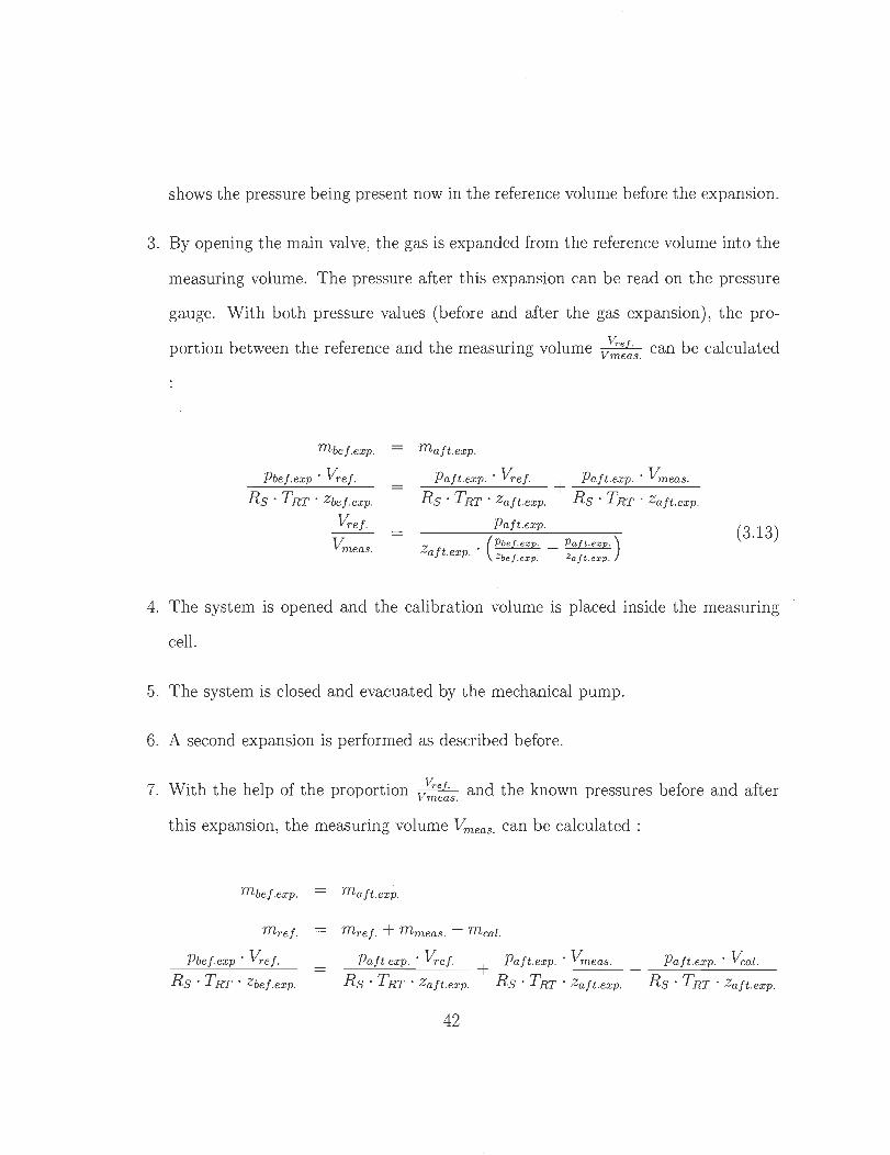
shows the pressure being present now in the reference volume before the expansion.
3. By opening the main valve, the gas is expanded from the reference volume into the
measuring volume. The pressure after this expansion can be read on the pressure
gauge. With both pressure values (before and after the gas expansion), the pro
portion between the reference and the measuring volume v';;;,:~s. can be calculated
mbef.exp. maft.exp.
Pbe f. exp . Vref. Paft.exp . . Vr ef. + Paft. exp.· Vm eas.
Rs . TRT . Za ft. exp. Rs . TRT . Zaft.exp . Rs . TRT . Zbef.exp.
Paft .exp.
Z . ( Pbef.exp. _ Patt. ex p.) aft.exp. Zbet.exp. Zatt. exp.
(3 .13) Vr ef.
Vmeas .
4. The system is opened and the calibration volume is placed inside the measuring
cell.
5. The system is closed and evacuated by the mechanical pump.
6. A second expansion is performed as described before.
7. With the help of the proportion v';;;,:~s. and the known pressures before and after
this expansion, the measuring volume Vm eas. can be calculated :
mbef.exp. maft.exp.
mref. mref. + mmeas. - mcal.
Pbef.exp . Vref. Paft.exp . . Vref. + Paft.exp. · Vm eas.
Rs . T RT . Zaft. exp. Rs . T RT . Za ft. exp.
Paft.exp . . Vcal.
Rs . TRT . Zbef.exp. Rs . T RT . Zaft.exp.
42
Vm eas. 1 -~ . ( Pbe /. eX p. ·zaft.exp. - 1) Vm eas . Zbef·exp. ·Paft.exp.
(3.14)
8. The reference volume Vref. can be calculated with the known proport ion v';;;,:~s . and
the measuring volume Vm eas ..
9. By repeating these steps e.g. 10 times, the measurements repeatability can be
checked and the final volumes can be determined by averaging the gained values.
3.2.3 Gravimetrie method
Another well-known method for t he determination of the gas uptake of a sample is t he
use of a magnetic suspension balance or a beam balance [26, 28, 29]. The gravimetric
determination of a samples gas uptake commonly has a few advantages in comparison to
the volumetrie determination [27] as described in subsection 3.2.1. These are in detail :
• The mass of the sample is measured directly. As a consequence, the calculation
of the amount of gas adsorbed on t he sample turns out to be very simple, instead
of calculating the amount adsorbed through pressures, temperatures and volumes,
just buoyancy effects have to be considered .
• The volumetrie method requires a fixed , known volume of aH pipes and valves
being installed in the system which means t hat every change or adaption of the
components used demands a complete recalibration of the system. A gravimetric
system does not show this disadvantage.
43
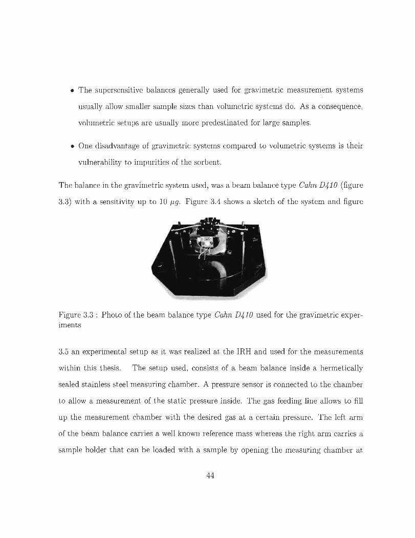
• The supersensitive balances generally used for gravimetric measurement systems
usually allow smaller sample sizes than volumetrie systems do. As a consequence,
volumetrie setups are usually more predestinated for large samples.
• One disadvantage of gravimetric systems compared to volumetrie systems is their
vulnerability to impurities of the sorbent.
The balance in the gravfmetric system used, was a beam balance type Cahn D410 (figure
3.3) with a sensitivity up to 10 P,9. Figure 3.4 shows a sketch of the system and figure
Figure 3.3 : Photo of the beam balance type Cahn D410 used for the gravimetric exp eriments
3.5 an experimental setup as it was realized at the IRH and used for the measurements
within this thesis. The setup used, consists of a beam balance inside a hermetically
sealed stainless steel measuring chamber. A pressure sensor is connected to the chamber
to allow a measurement of the static pressure inside. The gas feeding line allows to fill
up the measurement chamber with the desired gas at a certain pressure. The left arm
of the beam balance carries a weIl known reference mass whereas the right arm carries a
sample holder that can be loaded with a sample by opening the measuring chamber at
44
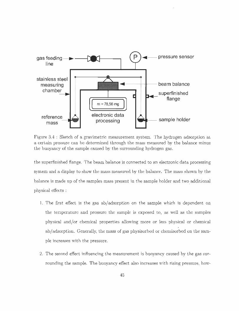
gas feeding-------..-~ line
stainless steel measuring chamber
reference -~-mass
....... .-- pressure sensor
~---+--t-- beam balance
( m = 78,56 mg )
electronic data processing
superfinished ------ flange
___ -- sample holder
Figure 3.4 : Sketch of a gravimetric measurement system. The hydrogen adsorption at a certain pressure can be determined through the mass measured by the balance minus the buoyancy of the sample caused by the surrounding hydrogen gas.
the superfinished fiange. The beam balance is connected to an electronic data processing
system and a display to show the mass measured by the balance. The mass shown by the
balance is made up of the samples mass present in the sample holder and two additional
physical effects :
l. The first effect is the gas ab/adsorption on the sample which is dependent on
the temperature and pressure the sample is exposed to, as well as the samples
physical and/or chemical properties allowing more or less physical or chemical
ab/adsorption. Generally, the mass of gas physisorbed or chemisorbed on the sam-
pIe increases with the pressure.
2. The second effect infiuencing the measurement is buoyancy caused by the gas sur-
rounding the sample. The buoyancy effect also increases with rising pressure, how-
45
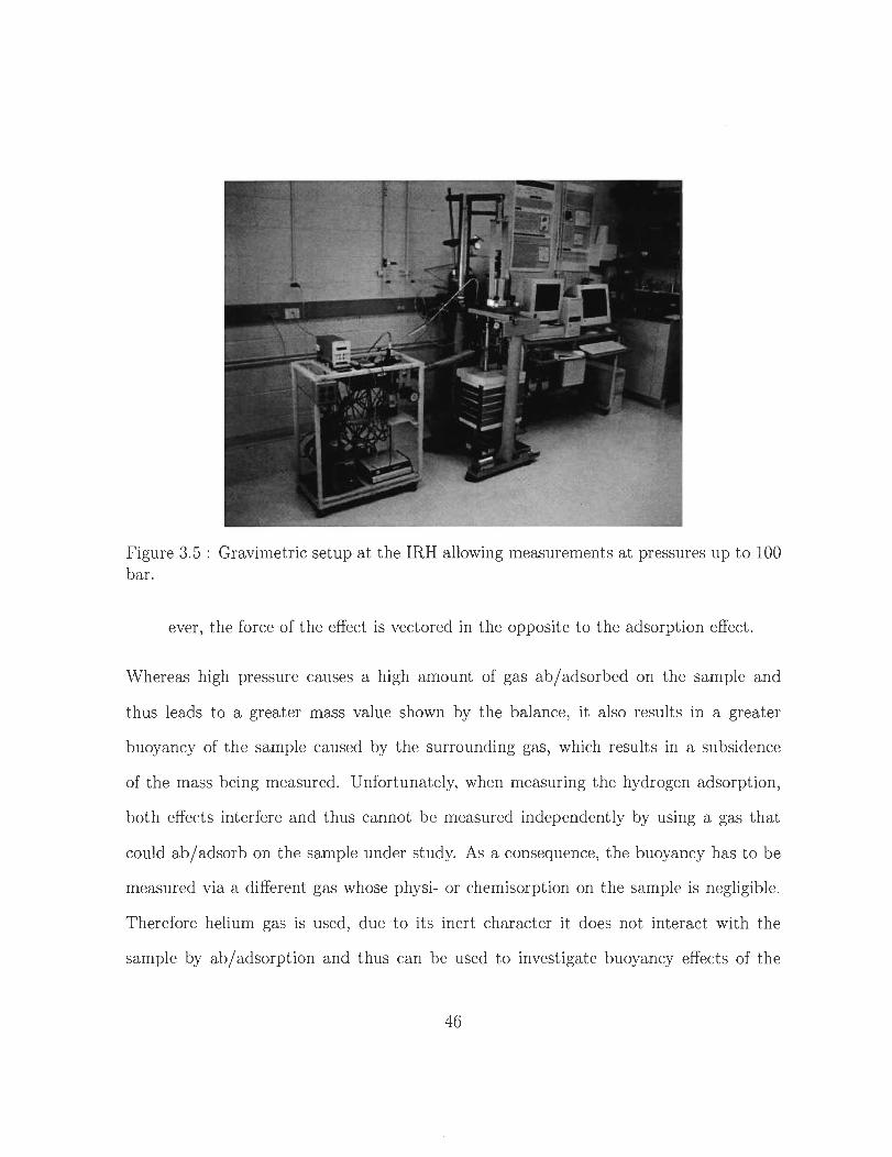
Figure 3.5 : Gravimetrie setup at the IRH allowing measurements at pressures up to 100 bar.
ever, the force of the effect is vectored in the opposite to the adsorption effect.
Whereas high pressure causes a high amount of gas ab/adsorbed on the sample and
thus leads to a greater mass value shown by the balance, it also results in a greater
buoyancy of the sample caused by the surrounding gas, whieh results in a subsidence
of the mass being measured. U nfortunately, when measuring the hydrogen adsorption,
both effects interfere and thus cannot be measured independently by using a gas that
could ab/adsorb on the sample under study. As a consequence, the buoyancy has to be
measured via a different gas whose physi- or chemisorption on the sample is negligible.
Therefore helium gas is used, due to its inert character it do es not interact with the
sample by ab/adsorption and thus can be used to investigate buoyancy effects of the
46
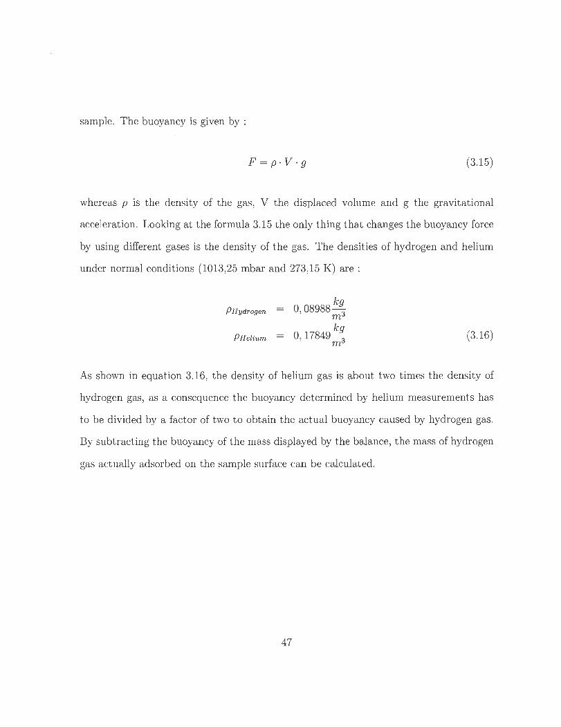
sample. The buoyancy is given by :
F=p·V·g (3.15)
whereas p is the density of the gas, V t he displaced volume and g the gravitational
acceleration. Looking at the formula 3.15 the only thing that changes the buoyancy force
by using different gases is the density of the gas. The densities of hydrogen and helium
under normal condit ions (1013,25 mbar and 273,15 K) are :
PHydrogen
PHelium
kg 0, 08988-
3 m kg
0, 17849-3 m
(3.16)
As shown in equation 3. 16, the density of helium gas is about two t imes t he density of
hydrogen gas, as a consequence the buoyancy determined by helium measurements has
to be divided by a factor of two to obtain t he açtual buoyancy caused by hydrogen gas.
By subtracting t he buoyancy of the mass displayed by the balance, the mass of hydrogen
gas actually adsorbed on the sample surface can be calculated .
47
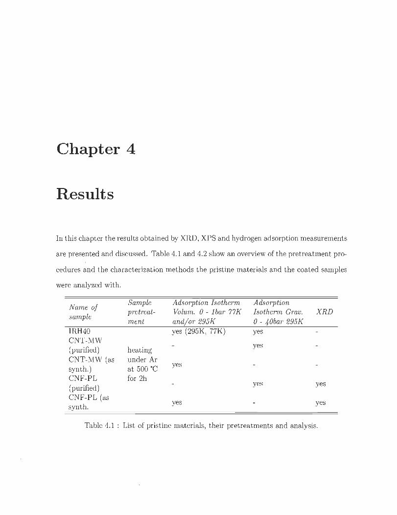
Chapter 4
Results
In this chapter the results obtained by XRD, XPS and hydrogen adsorption measurements
are presented and discussed. Table 4.1 and 4.2 show an overview of the pretreatment pro-
cedures and the characterization methods the pristine materials and the coated samples
were analyzed with.
Name of sample
IRH40 CNT-MW (purified) CNT-MW (as synth. ) CNF-PL (purified) CNF-PL (as synth.
Sample pretreatment
heating under Ar at 500 oC for 2h
Adsorption Isotherm Volum. 0 - 1 bar 77K and/ or 295K yes (295K, 77K)
yes
yes
Adsorption Isotherm Grav. XRD o - 40bar 295K yes
yes
yes yes
yes
Table 4.1 : List of pristine materials, their pretreatments and analysis.
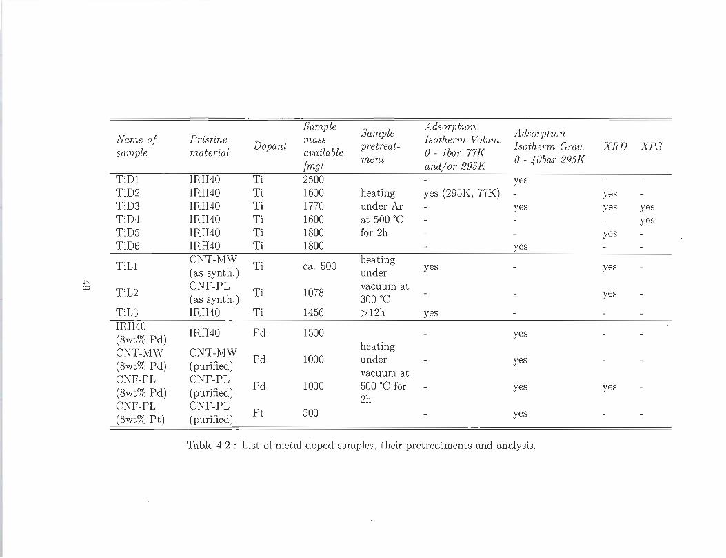
Sample Sample
Adsorption Adsorption
Name of Pristine Dopant
mass pretreat-
Isotherm Vol'Um. Isotherm Grav. XRD XPS
sample material available 0 - lbar 77K (mg)
ment and/or 295K
0 - 40bar 295K
TiD1 IRH40 Ti 2500 yes T iD2 IRH40 Ti 1600 heating yes (295K, 77K) yes TiD3 IRH40 T i 1770 under Ar yes yes yes T iD4 IRH40 T i 1600 at 500 oC yes TiD5 IRH40 Ti 1800 for 2h yes TiD6 IRH40 Ti 1800 yes
TiLl CNT-MW
Ti ca. 500 heating
(as synth.) under yes yes
..,. CNF-PL vacuum at CD T iL2 Ti 1078 (as synth.) 300 oC yes
TiL3 IRH40 Ti 1456 >12h yes IRH40
IRH40 Pd 1500 (8wt% Pd)
yes heating
CNT-MW CNT-MW (8wt% Pd) (purified)
Pd 1000 under yes vacuum at
CNF-PL CNF-PL Pd 1000 500 oC for
(8wt% Pd) (purified) yes yes
2h CNF-PL CNF-PL (8wt% Pt) (purified)
Pt 500 yes
Table 4.2 : List of metal doped samples, their pretreatments and analysis.
The following two sections describe the outcome of the analysis performed with the
titanium and the platinumjpalladium doped nano-carbons. All graphs mentioned are
included in the appendix.
4 .1 Results of nano-carbons used for doping pro-
cesses
• IRH40 (sample representing the pristine materials for experiments performed with
the CVDj PVD process and others). The in-house produced high surface area
activated carbon IRH40 of the IRH acts as a carbon support for most samples
produced. Offering a BET-surface area of about 2000 m 2 j g, its hydrogen adsorption
capacity nearly reaches 250 mljg at l bar and 77 K. Figures C.I, C.2, C.3 and C.4
show the adsorption isotherms for IRH40 at different temperatures and pressures.
The isotherms on figure C.3 and C.4 especially show the fully reversible desorption
process that proves the storage effect of hydrogen on IRH40 to be physisorption .
• CNT-MW (purified) (sample representing the pristine material for experiments
performed with colloidal microwave processing). The multi-walled carbon nan
otubes produced by FutureCarbon normally contain Co based catalysts as a holdover .
from their production process. These substances are removed through an adequate
HCI treatment. As shown in figure C.I , their hydrogen adsorption capacity reaches
0,8 gjkg at 40 bar and a temperature of 295 K which is around 4 times lower than
the capacity of IRH40 at the same conditions. This can be explained by their low
50
BET surface area of 200 m 2 / g.
• CNT-MW (as synth.) (sample representing the pristine material for experiments
performed with the wet chemical process). These CNT-MWs did not pass a HCl
treatment and should still contain small amounts of the met al catalysts used for
their production. As shown in figure A.2 no Co catalysts could be detected by
XRD.
• CNF-PL (purified) (sample representing the pristine material for experiments
performed with colloidal microwave processing). The carbon nanofibers platelet
type produced by FutureCarbon normally contain Fe based catalysts as a holdover
from their production process. These substances are removed through an adequate
HCl treatment. As shown in figure C.1, their hydrogen adsorption capacity reaches
0,5 g/ kg at 40 bar and a temperature of 295 K which is around 7 times lower than
the capacity of IRH40 at the same conditions. This can be explained by their low
BET surface area of 120 m 2 / g.
• CNF-PL (as synth.) (sample representing the pristine material for experiments
performed with the wet chemical process). These CNF-PLs did not pass a HCl
treatment and do still contain the metal catalysts used for their production. These
catalysts are not interfering with the chemicals used for the wet chemical doping .
approach.
51
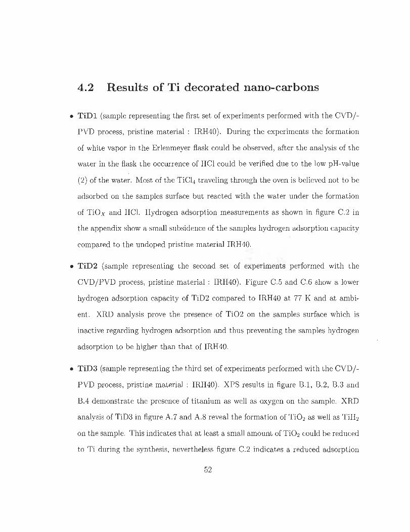
4.2 Results of Ti decorated nano-carbons
• TiD l (sample representing the first set of experiments performed with the CVD/
PVD process, pristine material : IRH40). During the experiments the formation
of white vapor in the Erlenmeyer fiask could be observed, after the analysis of the
water in the fiask the occurrence of HCI could be verified due to the low pH-value
(2) of the water. Most of the TiCl4 traveling through the oyen is believed not to be
adsorbed on the samples surface but reacted with the water under the formation
of TiO x and HCL Hydrogen adsorption measurements as shown in figure C.2 in
the appendix show a small subsidence of the samples hydrogen adsorption capacity
compared to the undoped pristine material IRH40.
• TiD2 (sample representing the second set of experiments performed with the
CVD/ PVD process, pristine material : IRH40). Figure C.5 and C.6 show a lower
hydrogen adsorption capacity of TiD2 compared to IRH40 at 77 K and at ambi
ent. XRD analysis prove the presence of Ti02 on the samples surface which is
inactive regarding hydrogen adsorption and thus preventing the samples hydrogen
adsorption to be higher than that of IRH40.
• TiD3 (sample representing the third set of experiments performed with the CVD/
PVD process, pristine material : IRH40). XPS results in figure B.I, B.2, B.3 and
B.4 demonstrate the presence of titanium as well as oxygen on the sample. XRD
analysis of TiD3 in figure A.7 and A.8 reveal the formation of Ti02 as well as TiH2
on the sample. This indicates that at least a small amount of Ti02 could be reduced
to Ti during the synthesis, nevertheless figure C.2 indicates a reduced adsorption
52
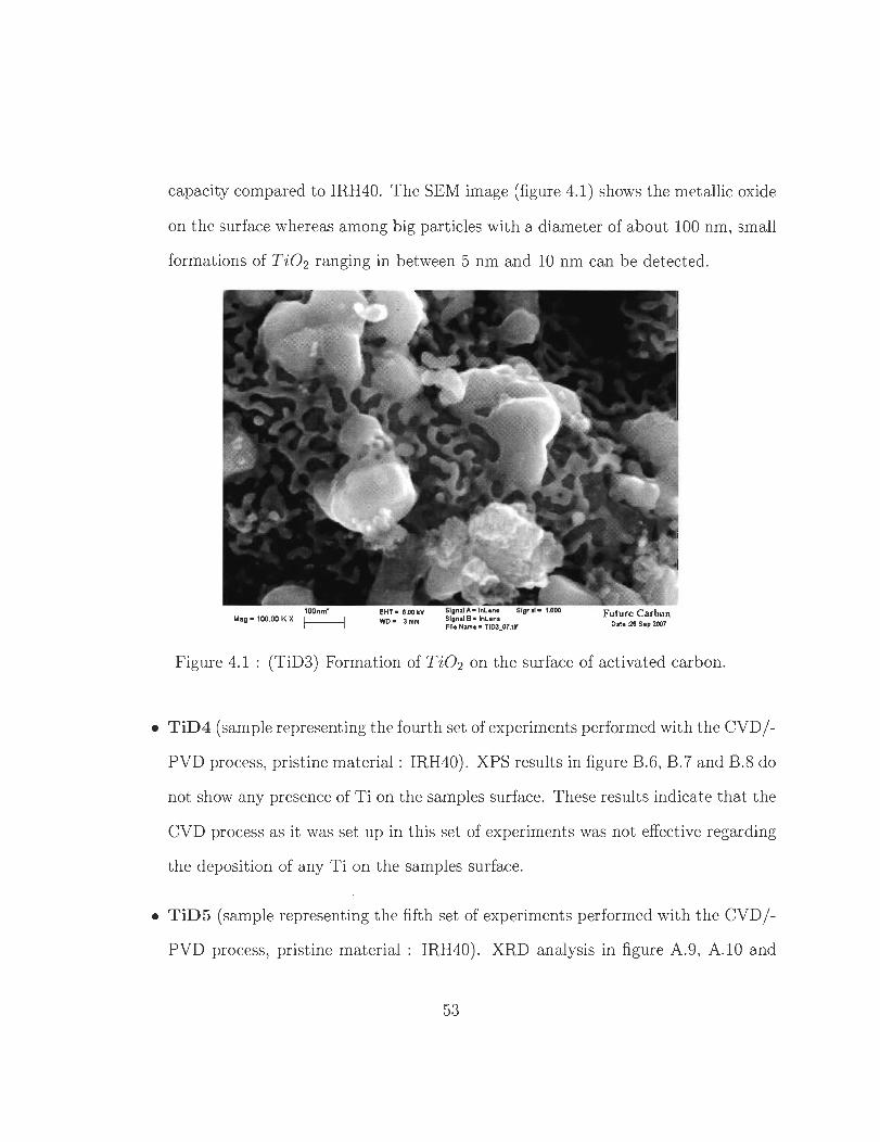
capacity compared to IRH40. The SEM image (figure 4.1) shows the metallic oxide
on the surface whereas among big particles with a diameter of about 100 nm, small
formations of Ti0 2 ranging in between 5 nm and 10 nm can be detected.
1OOnl11" Mag = 100.00 K X f-------1 EHT . ~.OO kV Signal A- tnLens Signal - 1.000
WC. 3 mm SlliInal B · tnLens Flle Nam.· T100_0T.ttI'
Future Carbon Dat. :26 Sep 2007
Figure 4.1 : (TiD3) Formation of Ti0 2 on the surface of activated carbon.
• TiD4 (sample representing the fourth set of experiments performed with the CVD /
PVD process, pristine materiai : IRH40). XPS results in figure B.6, B.7 and B.8 do
not show any presence of Ti on the samples surface. These results indicate that the
CVD process as it was set up in this set of experiments was not effective regarding
the deposition of any Ti on the samples surface .
• TiD5 (sample representing the fifth set of experiments performed with the CVD/
PVD process, pristine materiai : IRH40). XRD analysis in figure A.9, A.10 and
53
A.lI indicate the formation of different metal compounds like NiFe and CrFe as
well as Ti02 on the samples surface. The occurrence of metals can be explained
by a dissolution of the metal container which contained the sample through the
HCl, that was released during the synthesis. This met al contamination makes any
hydrogen adsorption measurement useless. Figure 4.2 shows the formation of a large
layer containing different metals on the surface of the activated carbon sample.
Figure 4.2 : (TiD5) Formation of different metals on the surface of the activated carbon sample .
• TiD6 (sample representing the sixth set of experiments performed with the CVD/
PVD process, pristine material : IRH40). Adsorption measurements of TiD6 in
figure C.2 indicate a decreased adsorption capacity compared to IRH40. Neverthe
less, the SEM image (figure 4.3) demonstrates the formation of nano-scaled T i 0 2
54
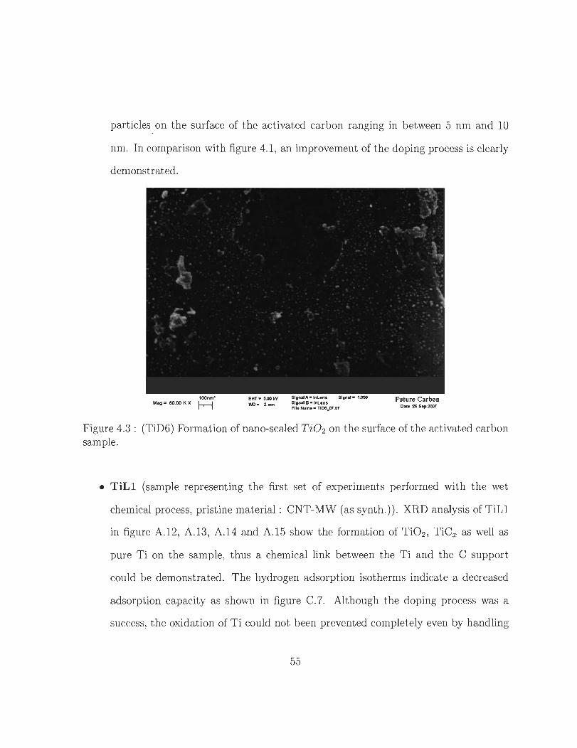
particles on the surface of the activated carbon ranging in between 5 nm and 10
nm. In comparison with figure 4.1, an improvement of the doping process is clearly
demonstrated.
100nma
Mag = 50.00 K X H EHT. 15.00 kV Sllnai A· InLens Signal - 1.000 WO • 2 mm Sllna' B • Inlens
Fil. Nam •• TI06_07.tif
Future Carbon Date:26 S.p 2007
Figure 4.3 : (TiD6) Formation of nano-scaled Ti02 on the surface of the activated carbon sample .
• TiLl (sample representing the first set of experiments performed with the wet
chemical process, pristine material : CNT-MW (as synth.)). XRD analysis of TiLl
in figure A.1 2, A.13, A.14 and A.15 show the formation of Ti02 , TiCx as well as
pure Ti on the sample, thus a chemical link between the Ti and the C support
could be demonstrated. The hydrogen adsorption isotherms indicate a decreased
adsorption capacity as shown in figure C.7. Although the doping pro cess was a
success, the oxidation of Ti could not been prevented completely even by handling
55
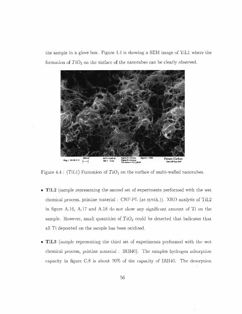
the sample in a glove box. Figure 4.4 is showing a SEM image of TiLl where the
formation of T i02 on the surface of the nanotubes can be clearly observed.
100nm" Mag= 50.00 K X H EHY - MOkV
wc- 3mm
Signal A. Inlens Signal- 1.000 Signai B • Inlen. Fil. Nam.· TIL 1_06.tIf
Future Carbon Date :26 Sep 2007
Figure 4.4 : (TiLl) Formation of Ti02 on the surface of multi-walled nanotubes .
• TiL2 (sample representing the second set of experiments performed with the wet
che mi cal process, pristine material : CNF-PL (as synth.)) . XRD analysis of TiL2
in figure A.l6 , A.l7 and A.l8 do not show any significant amount of Ti on the
sample. However, small quantities of Ti02 could be detected that indicates that
all Ti deposited on the sample has been oxidized .
• TiL3 (sample representing the third set of experiments performed with the wet
chemical process, pristine material : IRH40). The samples hydrogen adsorption
capacity in figure C.8 is about 70% of the capacity of IRH40. The desorption
56
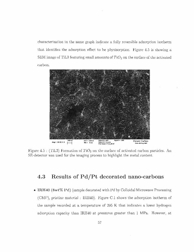
characterisation in the same graph indicate a fully reversible adsorption isotherm
that identifies the adsorption effect to be physisorption. Figure 4.5 is showing a
SEM image of TiL3 featuring small amounts of Ti02 on the surface of the activated
carbon.
100nma
Mag= 60.00 K X H EHT - 5.00 kV WO- 3 mm
Signai A· SE2 Signai- 1.000 Signal B· InLens File Nam •• TiL2_08.tif
Future Carbon Date:26 Sep 2007
Figure 4.5 : (TiL3) Formation of Ti02 on the surface of activated carbon particles. An SE-detector was used for the imaging process to highlight the metal .content.
4.3 Results of Pd/Pt decorated nano-carbons
• IRH40 (8wt% Pd) (sample decorated with Pd by Colloidal Microwave Processing
(CMP), pristine material : IRH40). Figure C.I shows the adsorption isotherm of
the sample recorded at a temperature of 295 K that indicates a lower hydrogen
adsorption capacity than IRH40 at pressures greater than l MPa. However, at
57
low pressures up to 1 MPa the adsorption capacity exceeds the one of IRH40 a
litt le bit. Both isotherms intersect at a pressure of 1 MPa. The small bend of
the isotherm can be explained by the formation of palladium-hydride that already
occures at very low pressures. This advantage in st orage capacity decreases with
increasing pressure and turns into a disadvantage at pressures greater than 1 bar
where the palladium is saturated with hydrogen and more or less inactive for further
hydrogen storage. The adsorption process can be fully explained by physisorption
on the surface of the carbon and chemisorption on the palladium .
• CNT-MW (8wt% Pd) (sample decorated with Pd by Colloidal Microwave Pro
cessing (CMP), pristine material : CNT-MW (purified)) . Figure C.1 shows the
adsorption isotherm of the sample recorded at a temperature of 295 K that indi
cates an increased hydrogen adsorption capacity in the whole pressure range up to
4 MPa. The isotherm also indicates a small bend at a pressure of 0,1 MPa which
attests the formation of palladium hydride. Nevertheless, the slope of the isotherm
is slightly lower compared to the isotherm of the pristine material. The point of
intersection is believed to be at high pressures of about 10 MPa. The adsorption
pro cess can be fully explained by physisorption on the surface of the carbon and
chemisorption on the palladium .
• CNF-PL (8wt% Pd) (sample decorated with Pd by Colloidal Microwave Process
ing (CMP) , pristine material: CNF-PL (purified)) Figure C.1 shows the adsorption
isotherm of the sample recorded at a temperature of 295 K that also indicates an
increased adsorption capacity in the whole pressure range recorded. The slope of
58
the isotherm is clearly lower compared to the isotherm of the pristine material, t he
point of intersection should be located around 6 MPa. The adsorption pro cess can
be fully explained by physisorption on the surface of the carbon and chemisorp
tion on the palladium. Figure A.l shows an X-ray diffractogramm of the sample
identifying the palladium on the samples surface
• CNF-PL (8wt% Pt) (sample decorated with Pt by Colloidal Microwave Pro
cessing (CMP) , pristine material: CNF-PL (purified)). Figure C.l shows the
adsorption isotherm of the sample recorded at a temperature of 295 K that gener
ally indicates the same behaviour as the isotherm of the palladium coated sample.
The only difference is the bend of the isotherm which is occuring at 0,1 MPa due to
the different formation process of platinum hydride. AlI adsorption pro cesses can
be explained by physisorption and chemisorption.
59
Chapter 5
Adsorption measurements at
temperatures from 30 K to 77 K
As already stated in the summery, an additional part of the thesis was to modify an
existing volumetrie measurement system in order to allow the recording of adsorption
isotherms at temperatures between 30 K and 77 K. In this temperature range, liquid
nitrogen is no longer suitable as a cooling agent, as a consequence liquid helium has to
be used. The work performed in this field will be published as a scientific article in an
renowned journal, the following pages show a draft of this article explaining the work
done so far and the results gained.
60
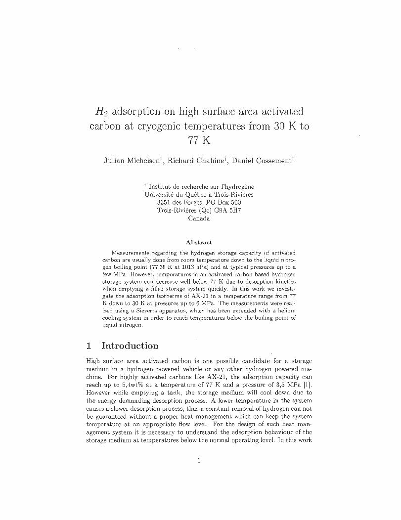
H2 adsorption on high surface area activated carbon at cryogenie temperatures from 30 K to
77 K
Julian Michelsen t, Richard Chahine t, Daniel Cossement t
t Institut de recherche sur l'hydrogène Université du Québec à Trois-Rivières
3351 des Forges, PO Box 500 Trois-Rivières (Qc) G9A 5H7
Canada
Abstract
Measurements regarding t he hydrogen storage capacity of activated carbon are usually done from room temperature down to the liquid nitrogen boiling point (77,35 K at 1013 hPa) and at typical pressures up to a few MPa. However, temperatures in an activated carbon based hydrogen storage system can decrease weil below 77 K due to desorption kinetics when emptying a filled storage system quickly. In this work we investigate the adsorption isotherms ofAX-21 in a temperature range from 77 K down to 30 K at pressures up to 6 MPa. The measurements were realized using a Sieverts apparatus, which has been extended with a helium cooling system in order to reach temperatures below the boiling point of liquid nitrogen.
1 Introduction
High surface area activated carbon is one possible candidate for a storage medium in a hydrogen powered vehicle or any other hydrogen powered machine. For highly activated carbons like AX-21, the adsorption capacity can reach up to 5,4wt% at a temperature of 77 K and a pressure of 3,5 MPa [1]. However while emptying a tank, t he storage medium will cool down due to the energy demanding desorption process. A lower temperature in the system causes a slower desorption process, t hus a constant removal of hydrogen can not be guaranteed without a proper heat management which can keep the system temperature at an appropriate flow level. For the design of such heat management system it is necessary to understand t he adsorption behaviour of the storage medium at temperatures below the normal operating level. In t his work
1
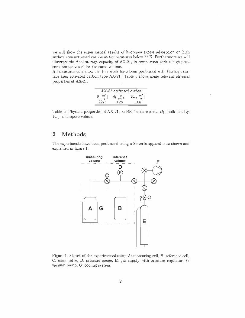
we will show the experimental results of hydrogen excess adsorption on high surface area activated carbon at temperatures below 77 K. Furthermore we will illustrate the final storage capacity ofAX-21, in comparison with a high pressure storage vessel for the same volume. All measurements shown in this work have been performed with the high surface area activated carbon type AX-21. Table 1 shows sorne relevant physical properties of AX-21.
AX-21 activated carbon
S 1r;3] dbl~] Vmp lr;3] 2278 0,28 1,06
Table 1: Physical properties ofAX-21. S: BET-surface area. Db: bulk density. Vmp : micropore volume.
2 Methods
The experiments have been performed using a Sieverts apparatus as shown and explained in figure 1.
measuring volume
reference volume
E
Figure 1: Sketch of the experimental setup A: measuring cell, B: reference cell, C: main valve, D: pressure gouge, E: gas supply with pressure regulator, F: vacuum pump, G: cooling system.
2
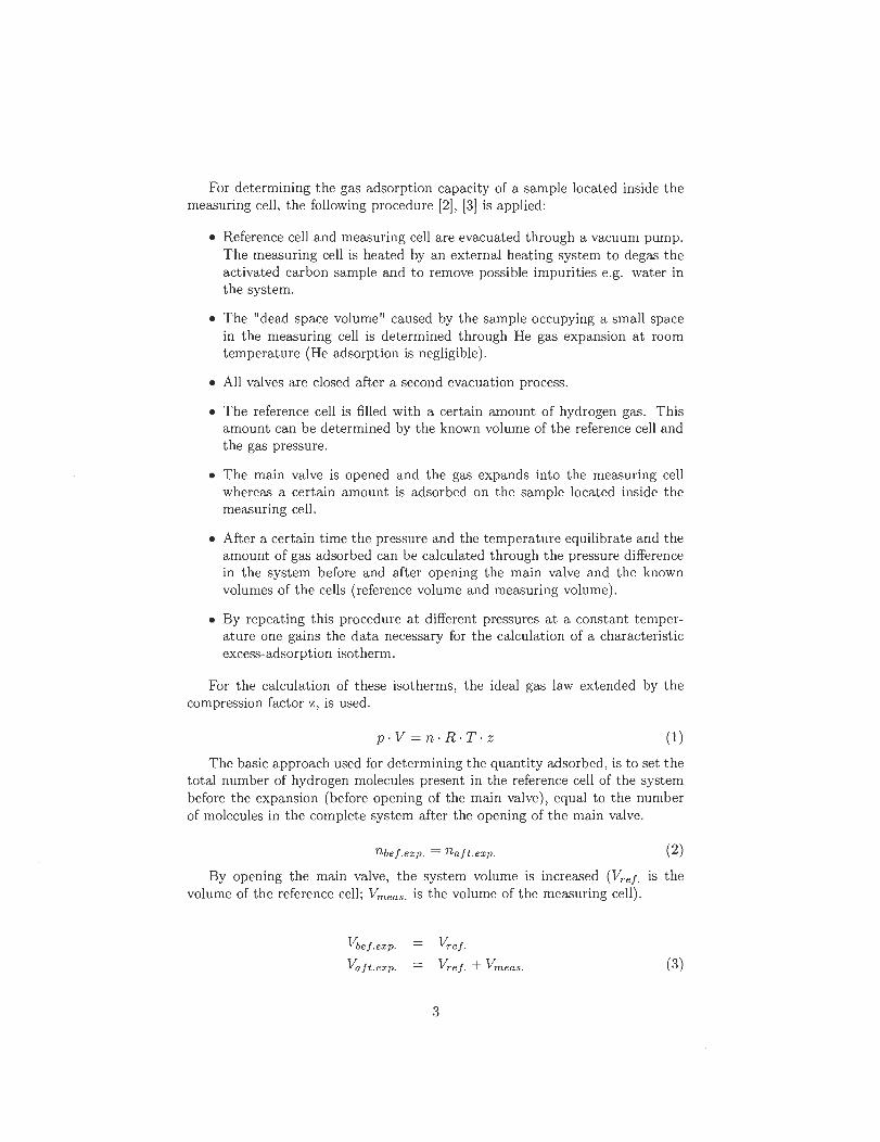
For determining the gas adsorption capacity of a sam pIe located inside the measuring cell, the following procedure [2], [31 is applied:
• Reference cell and measuring cell are evacuated through a vacuum pump. The measuring cell is heated by an external heating system to degas the activated carbon sam pIe and to remove possible impurities e.g. water in the system.
• T he "dead space volume" caused by the sample occupying a small space in the measuring cell is determined through He gas expansion at room temperature (He adsorption is negligible).
• All valves are closed after a second evacuation process.
• T he reference cell is filled with a certain amount of hydrogen gas. This amount can be determined by the known volume of the reference cell and t he gas pressure.
• T he main valve is opened and the gas expands into the measuring cell whereas a certain amount is adsorbed on the sample located inside the measuring cell .
• After a certain time the pressure and the temperature equilibrat e and the amount of gas adsorbed can be calculated through the pressure difference in t he system before and after opening the main valve and t he known volumes of the cells (reference volume and measuring volume).
• By repeating this procedure at different pressures at a constant temperature one gains the data necessary for the calculation of a characteristic excess-adsorption isotherm.
For the calculation of these isotherms, the ideal gas law extended by the compression factor z, is used.
p ·V=n·R·T·z (1)
T he basic approach used for determining the quantity adsorbed, is to set the total number of hydrogen molecules present in the reference cell of the system before t he expansion (before opening of the main valve) , equal to the number of molecules in the complete system after the opening of the main valve.
nbe f.e x p. = naft.exp. (2)
By opening the main valve, the system volume is increased (Vref. is the volume of the reference cell ; V m eas . is the volume of the measuring cell) .
Vbe f .ex p. Vref.
Vaft .exp. Vref. + V meas . (3)
3
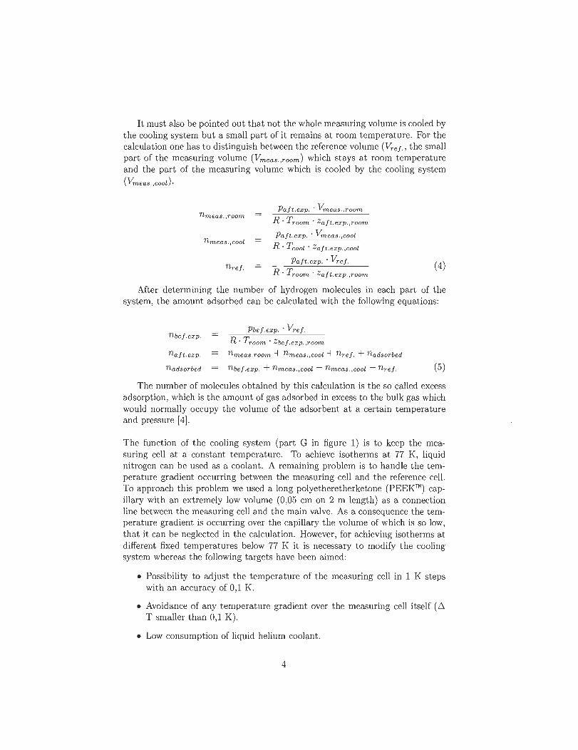
It must also be pointed out that not the whole measuring volume is cooled by the cooling system but a small part of it remains at room temperature. For the calculation one has to distinguish between the reference volume (Vre f. , the small part of the measuring volume (Vmeas . ,room) which stays at room temperature and the part of the measuring volume which is cooled by the cooling system (Vmeas. ,cool).
nmeas . ,room
nmeas.,cool
Paft .exp . . Vrneas. ,roorn
R . Troorn . Zaft.exp.,roorn
P aft. exp . . Vrneas. ,cool
R· Tcool . Zaft .exp .,cool.
Paft.exp . . V ref.
R· Troorn . Zaft.exp. ,roorn (4)
After determining the number of hydrogen molecules in each part of the system, the amount adsorbed can be calculated with the following equations:
nbe f ·exp.
naft.exp.
nadsorbed
Pbe f. exp . . Vre f.
R . Tr oorn . z bef.ex p. ,room
nrneas.roorn + nrneas. ,cool + nref. + nadsorbed
nbef.exp. + nmeas. ,cool - nrneas. ,cool - nref. (5)
The number of molecules obtained by this calculation is the so called excess adsorption, which is the amount of gas adsorbed in excess to the bulk gas which would normally occupy the volume of the adsorbent at a certain tempe rature and pressure [4] .
The function of the cooling system (part G in figure 1) is to keep the measuring cell at a constant temperature. To achieve isotherms at 77 K, liquid nitrogen can be used as a coolant. A remaining problem is to han dIe the temperature gradient occurringbetween the measuring cell and the reference cell. To approach this problem we used a long polyetheretherketone (PEEK™) capillary with an extremely low volume (0 ,05 cm on 2 m length) as a connection line between the measuring cell and the main valve. As a consequence the temperature gradient is occurring over the capillary the volume of which is so low, that it can be neglected in the calculation. However, for achieving isotherms at different fixed temperatures below 77 K it is necessary to modify the cooling system whereas the following targets have been aimed:
• Possibility to adjust the temperature of the measuring cell in 1 K steps with an accuracy of 0,1 K.
• Avoidance of any temperature gradient over the measuring cell itself (.6 T smaller than 0,1 K).
• Low consumption of liquid helium coolant.
4
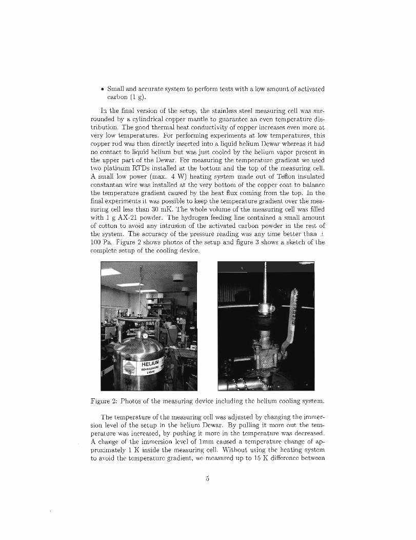
• Small and accurate system to perform tests with a low amount of activated carbon (1 g).
In the final version of the setup, the stainless steel measuring cell was surrounded by a cylindrical copper mantle to guarantee an even temperature distribution. The good thermal heat conductivity of copper increases even more at very low temperatures. For performing experiments at low temperatures, this copper rod was then directly inserted into a liquid helium Dewar whereas it had no contact to liquid helium but was just cooled by the helium vapor present in the upper part of the Dewar. For measuring the temperature gradient we used two platinum RTDs installed at the bottom and the top of the measuring cell. A small low power (max. 4 W) heating system made out of Teflon insulated constantan wire was installed at the very bottom of the copper coat to balance the temperature gradient caused by the heat flux coming from the top. In the final experiments it was possible to keep the temperature gradient over the measuring celliess than 30 mK. The whole volume of the measuring cell was filled with 1 g AX-21 powder. The hydrogen feeding line contained a small amount of cotton to avoid any intrusion of the activated carbon powder in the rest of the system. The accuracy of the pressure reading was any time better than ± 100 Pa. Figure 2 shows photos of the setup and figure 3 shows a sketch of the complete setup of the cooling device.
Figure 2: Photos of the measuring device including the helium cooling system.
The temperature of the measuring cell was adjusted by changing the immersion level of the setup in the helium Dewar. By pulling it more out the temperature was increased, by pushing it more in the temperature was decreased. A change of the immersion level of 1mm caused a temperature change of approximately 1 K inside the measuring cell. Without using the heating system to avoid the temperature gradient, we measured up to 15 K difference between
5
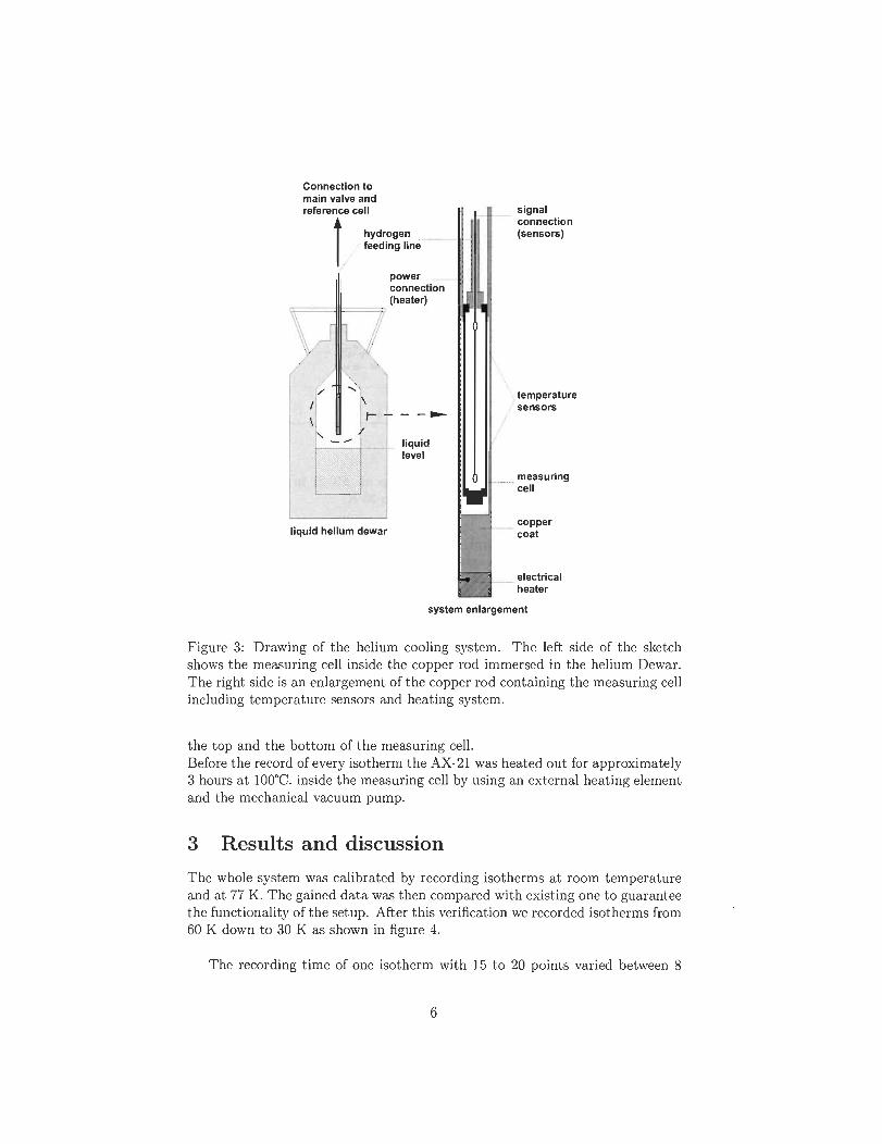
Connection to main valve and reference cell
t /.. :;:d':,~·':"'
'i'r==III==~
liquid helium dewar
power connection (heater)
- --liquid level
signal ..... . ........... connection
(sensors)
, temperature . sensors
measuring ....... cell
copper ............ coat
............ electrical heater
system enlargement
F igure 3: Drawing of the helium cooling system. The left si de of the sketch shows t he measuring cell inside the copper rod immersed in t he helium Dewar. T he right side is an enlargement of the copper rod containing the measuring cell including temperature sensors and heating syst em.
t he top and the bottom of the measuring cell. Before t he record of every isotherm the AX-21 was heated out for approximately 3 hours at 1000e. inside the measuring cell by using an external heating element and the mechanical vacuum pump.
3 Results and discussion
The who le system was calibrated by recording isotherms at room temperature and at 77 K. The gained data was then compared with existing one to guarantee the functionality of t he setup. After this verification we recorded isotherms from 60 K down to 30 K as shown in figure 4.
T he recording time of one isotherm with 15 to 20 points varied between 8
6
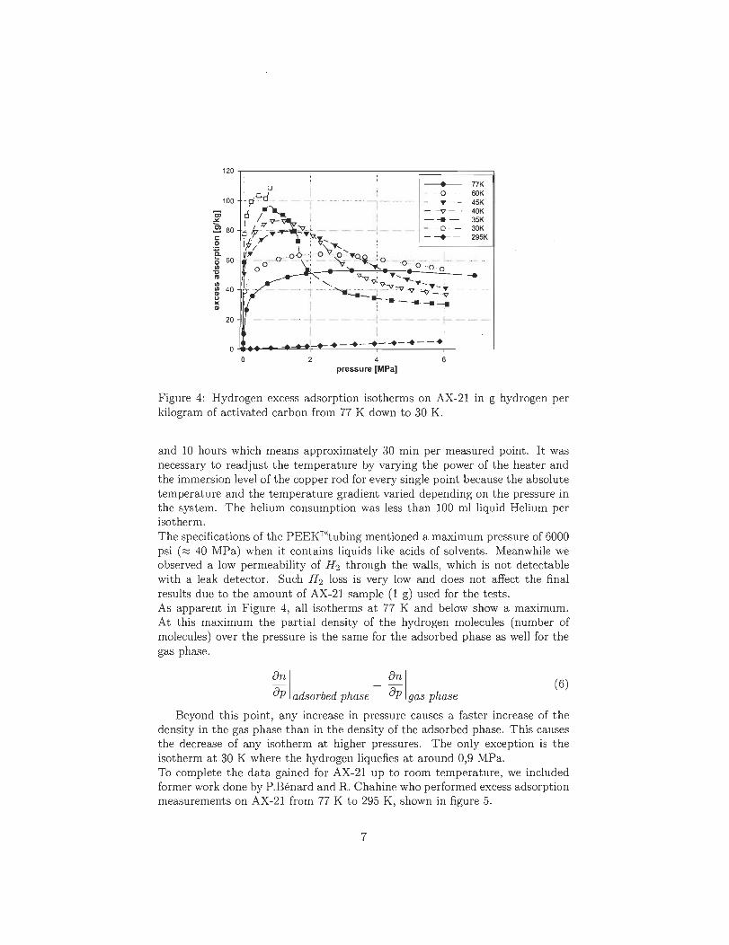
120
100
Ci -" ~ 80 c 0
~ 5 60 1/)
" co 1/) 1/) 40 CI> (J
>< CI>
20
o 2
~<~- f<-< --<- <-<- -<-
.-~-~-~-·--·i 4
pressure [MPa] 6
Figure 4: Hydrogen excess adsorption isotherms on AX-21 in g hydrogen per kilo gram of activated carbon from 77 K down to 30 K.
and 10 ho urs which means approximately 30 min per measured point. It was necessary to readjust the temperature by varying the power of the heater and the immersion level of the copper rod for every single point because the absolute temperature and the temperature gradient varied depending on the pressure in the system. The helium consumption was less than 100 ml liquid Helium per isotherm. The specifications of the PEEK™tubing mentioned a maximum pressure of 6000 psi (~ 40 MPa) when it contains liquids like acids of solvents. Meanwhile we observed a low permeability of H 2 through the walls , which is not detectable with a leak detector. Such H 2 loss is very low and does not affect the final results due to the amount ofAX-21 sample (1 g) used for the tests. As apparent in Figure 4, all isotherms at 77 K and below show a maximum. At this maximum the partial density of the hydrogen molecules (number of molecules) over the pressure is the same for the adsorbed phase as well for the gas phase.
ânl âp adsorbed phase
ân l âp gas phase
(6)
Beyond this point , any increase in pressure causes a faster increase of the density in the gas phase than in the density of the adsorbed phase. This causes the decrease of any isotherm at higher pressures. The only exception is the isotherm at 30 K where the hydrogen liquefies at around 0,9 MPa. To complete the data gained for AX-21 up to room temperature, we included former work done by P.Bénard and R. Chahine who performed excess adsorption measurements on AX-21 from 77 K to 295 K , shown in figure 5.
7
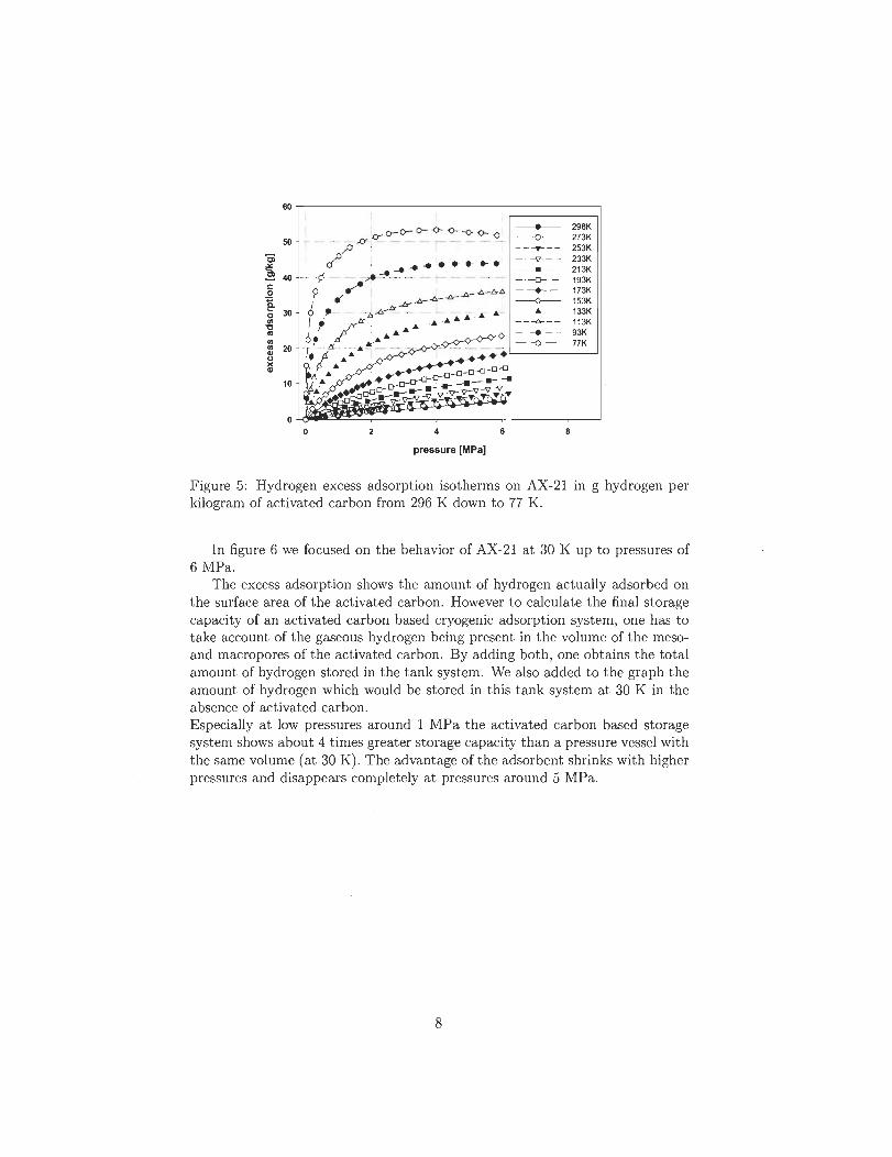
60
50 .,.
Ci "" ~ 40 c 0
:a Cs 30
'" " co
'" '" 20 CI> u .. CI>
10
0 2 4
pressure [MPa)
6
• 298K . o ·· 273K
-- --T- -- 253K - .. -v._ .- 233K ----- .-0-- ---------<>--... . ----6---- ---._-
213K 193K 173K 153K 133K 113K 93K
- --0 - 77K
Figure 5: Hydrogen excess adsorption isotherms on AX-21 in g hydrogen per kilogram of activated carbon from 296 K down to 77 K.
In figure 6 we focused on the behavior ofAX-21 at 30 K up to pressures of 6 MPa.
The excess adsorption shows the amount of hydrogen actually adsorbed on the surface area of the activated carbon. However to calculate the final storage capacity of an activated carbon based cryogenie adsorption system, one has to take account of the gaseous hydrogen being present in the volume of the mesoand macro pores of the activated carbon. By adding both, one obtains t he total amount of hydrogen stored in the tank system. We also added to the graph the amount of hydrogen which would be stored in this tank system at 30 K in the absence of activated carbon. Especially at low pressures around 1 MPa the activated carbon based storage system shows about 4 times greater storage capacity than a pressure vessel with the same volume (at 30 K) . The advantage of the adsorbent shrinks with higher pressures and disappears completely at pressures around 5 MPa.
8
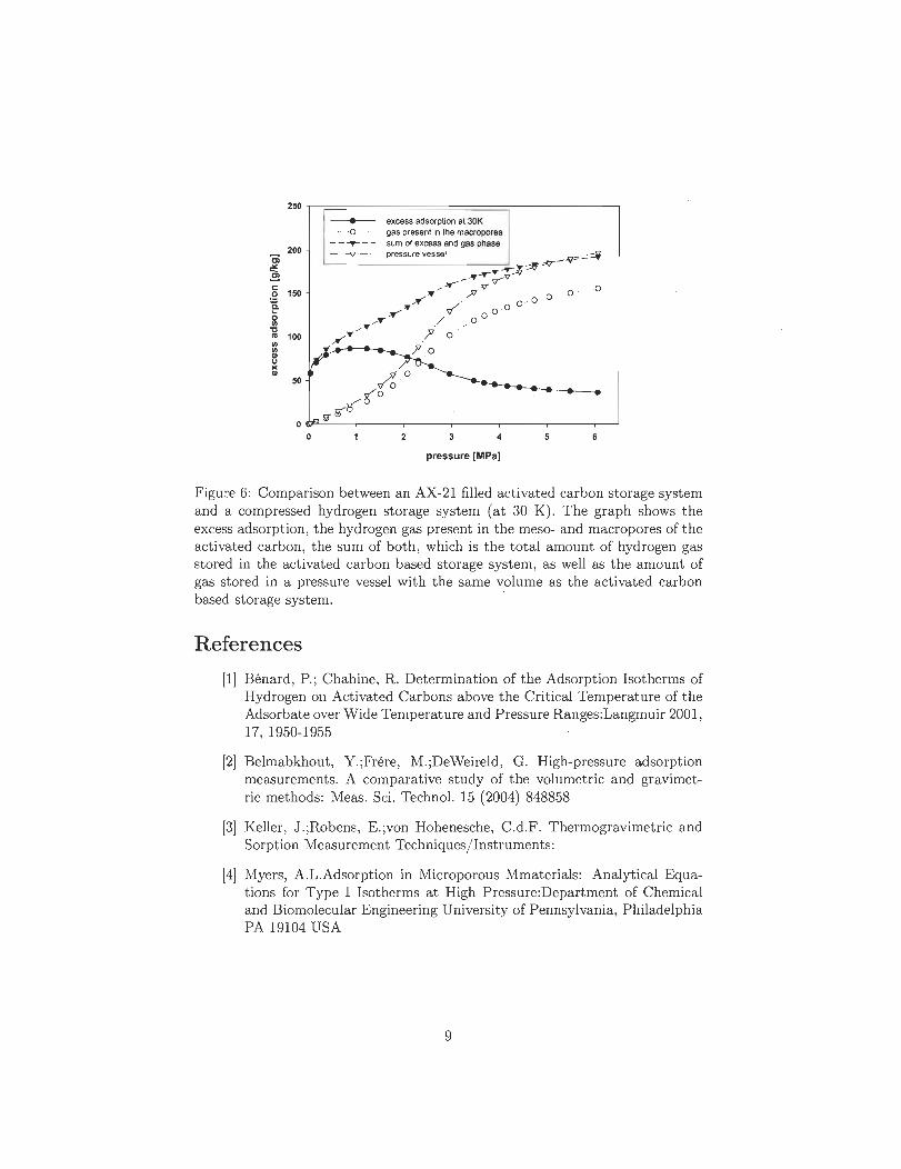
250~~======================~----------~
200 Ci -'" S g 150
a o '" "t:I co 100
'" '" .. u .. ..
50
___ excess adsorption at 30K .. . 0 gas present in the macropores
- - -T- - - sum of excess and gas phase _ . -V ' - pressure vessel ~ ___ ~
L---------------------~--r--:! ~ ~""-
-~ V-" _~ V 0
A"Y . fi 00 ° 0 ..-Y if 0 0 Y _ "- / . 00
A"Y- ? 0
2 3 4 5
pressure [MPa]
Figure 6: Comparison between an AX-21 filled activated carbon storage system and a compressed hydrogen storage system (at 30 K). The graph shows the excess adsorption, the hydrogen gas present in the mesa- and macropores of the activated carbon, the sum of both, which is the total amount of hydrogen gas stored in the activated carbon based storage system, as well as the amount of gas stored in a pressure vessel with the same volume as the activated carbon based storage system.
References
[1] Bénard, P.; Chahine, R. Determination of the Adsorption Isotherms of Hydrogen on Activated Carbons above the Critical Temperature of the Adsorbate over Wide Temperature and Pressure Ranges:Langmuir 2001 , 17, 1950-1955
[2] Belmabkhout, Y;Frére, M.;DeWeireld, G. High-pressure adsorption measurements. A comparative study of the volumetric and gravimetric methods: Meas. Sei. Technol. 15 (2004) 848858
[3] Keller, J.;Robens, E.;von Hohenesche, C.d.F. Thermogravimetric and Sorption Measurement Techniques/ Instruments:
[4] Myers, A.L.Adsorption in Microporous Mmaterials: Analytical Equations for Type 1 Isotherms at High Pressure:Department of Chemical and Biomolecular Engineering University of Pennsylvania, Philadelphia PA 19104 USA
9
Chapter 6
Conclusion
The procedures and techniques used for the metal doping of the nano-carbon materials
were basically working. Both methods used for the synthesis of titanium doped materials
(CVD/PVD and wet chemical method) turned out to be suitable for depositing titanium
on the surface of the samples, however, the pro cesses were linked with difficulties :
1. The CVD /PVD pro cess just allowed a poor control of the amount of titanium being
deposited and thus, over the thickness of the titanium layer on the samples surface.
XRD measurements show that the thickness of that layer sometimes reached more
than 100 molecule diameters which is way too mu ch for proving the increased
hydrogen storage effect as it was predicted by [2] and [3].
2. The greatest problem concerning the titanium coating technologies turned out to be
the formation of solid Ti02 during or after the synthesis. In the CVD /PVD Ti02
was produced intentionally to obtain a solid phase on the surface of the sample,
however, the reduction of that substance was hardly possible without destroying
the molecular structure of the sample. As a consequence just a fraction of the
Ti02 could be turned into pure titanium. Additionally, pure titanium immediately
oxidizes in an ambient atmosphere, so the samples had to be prepared for analysis
inside a glove-box. Even inside the glove-box, which was filled with argon gas and
usually showed an oxygen concentration of maximum 300 ppm, the titanium did
oxidize after a few days.
one of the hydrogen adsorption measurements of the samples decorated with titanium
did show an increased adsorption capacity which can be explained by the formation of
Ti02 that occurred intentionally during the synthesis or as soon as the sample was ex
posed to small quantities of oxygen. The presence of Ti02 could be proven by XRD as
well as XPS analysis for most of the samples. Due to the inactivity of Ti02 regarding
hydrogen adsorption the coating acted as a ballast , the remaining adsorption capacity
can be fully explained by physisorption on the samples surface. A storage effect as de
scribed by [2, 3, 4] could not be generated.
Decorating nano-carbons with noble met aIs like palladium and platinum by Colloidal
Microwave Processing allowed a better control of the amount of metal deposited on the
samples surface. Hydrogen adsorption measurements of samples decorated with palla
dium or platinum. showed an increasing of their adsorption capacity after the doping
process. However, two important points have to be considered :
1. The adsorption isotherms of the metal doped materials usually shows a bend at low
pressures around 1 bar up to witch the adsorption capacity rises very fast. This
behavior can be explained by the formation of metal hydrides (palladiumjplatinum
71
hydride) which already get saturated at low pressures. At pressures greater 1bar,
the additional adsorption is caused by physisorption on the remaining surface of
the sample.
2. The slope of the adsorption isotherms of the metal decorated materials is, at pres
sures greater 1 bar, lower in comparison with the undoped pristine materials. De
pending on the doping and the pristine material the adsorption isotherms of both,
the doped material and same material undoped, intersect at a certain pressure. At
this pressure the adsorption capacity of the undoped pristine material gets higher
than the capacity of the doped one.
The adsorption effects measured can be fully explained by simple chemi- and physisorp
tion. A spillover effect as it was mentioned by [13, 14J could not be measured.
Future work in this field should aim at adapting the methods developed for the dop
ing pro cess in order to gain a better control of the metal layer deposited on the samples
surface. In case of the titanium doping, efforts have to be made to prevent an oxidation
of the sample by preventing any contact with oxygen.
72
Appendix A
XRD results
73
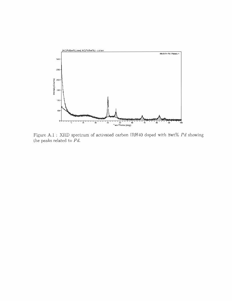
065-6174> Pd · Palladium
3000
2500
1000
500
10 20 30 40 50 60 90 100
Two-Theta (deg)
Figure A.l : XRD spectrum of activated carbon IRH40 doped with 8wt% Pd showing the peaks related to Pd_
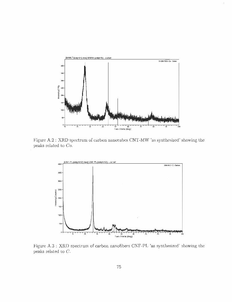
Two-Theta (deg)
Figure k2 : XRD spectrum of carbon nanotubes CNT-MW 'as synthesized' showing the peaks related to Co.
4~~~~~~~~~~~~~~-------------------------------' 026-1077> C-Carbon
3500
3000
_ 2500
'" ë i5 ~2OOJ .~
Ë 1500
500
10 20 30 40 50" 60 70 BQ 90 100
Two-Theta (deg)
Figure A.3 : XRD spectrum of carbon nanofibers CNF-PL 'as synthesized' showing the peaks related to C.
75
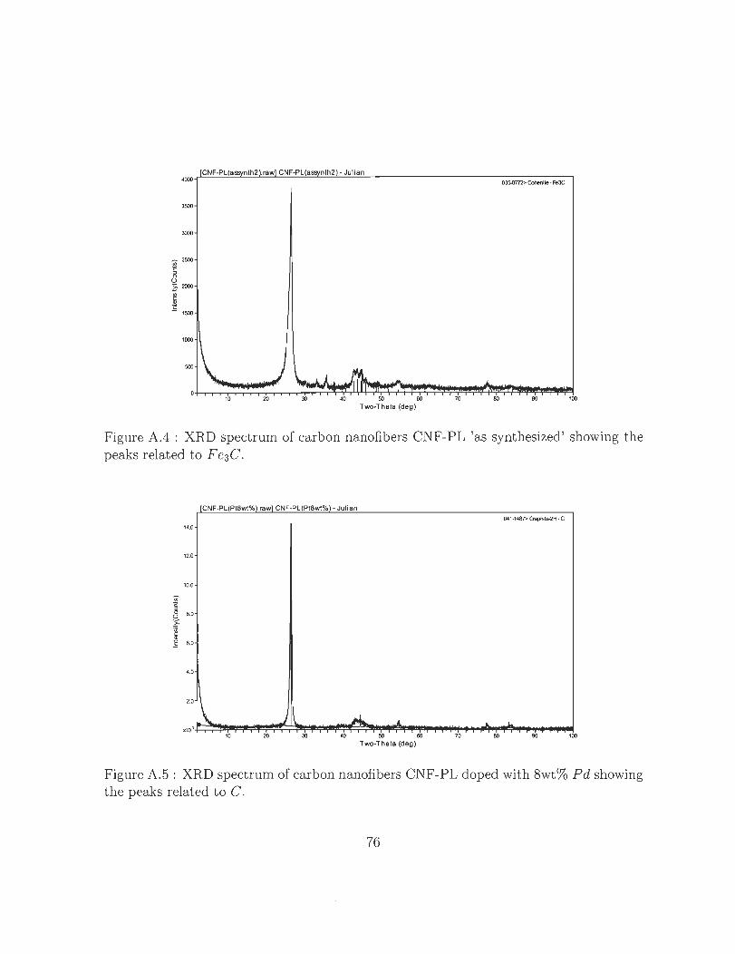
3500
500
10 20 30 40 50 60 70 80 90 100
Two-Thela (deg)
Figure A.4 : XRD spectrum of carbon nanofibers CNF-PL 'as synt hesized ' showing the peaks related to F e3C.
[CNF-PL(PI8wt%).raw] CNF-PL(PI8wt%) - Ju li an 04 1-1487> Gaphite-2H-C
14 .0
12.0
10.0
~ BO
·_-c~ 6.0
4.0
2.0 \.
.1 .. ><1 0 '
10 20 30 40 50 60 70 80 90 100
Two-Thela (deg)
Figure A. 5 : XRD spectrum of carbon nanofibers CNF-PL doped with 8wt% P d showing the peaks related to C.
76
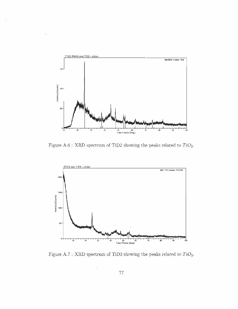
()()()..{)()()8 Anatase-li02
7fil
2fil
20 30 40 fil 60 70 60 90 100
Two-Theta (d eg)
Figure A.6 XRD spectrum of TiD2 showing the peaks related to Ti02 .
086-1157> Anatase - liO. nC12
2000
1500
500
10 20 30 40 50 60 70 80 90 100
Two-Theta (deg)
Figure A.7 : XRD spectrum of TiD3 showing t he peaks related to T i 0 2 .
77
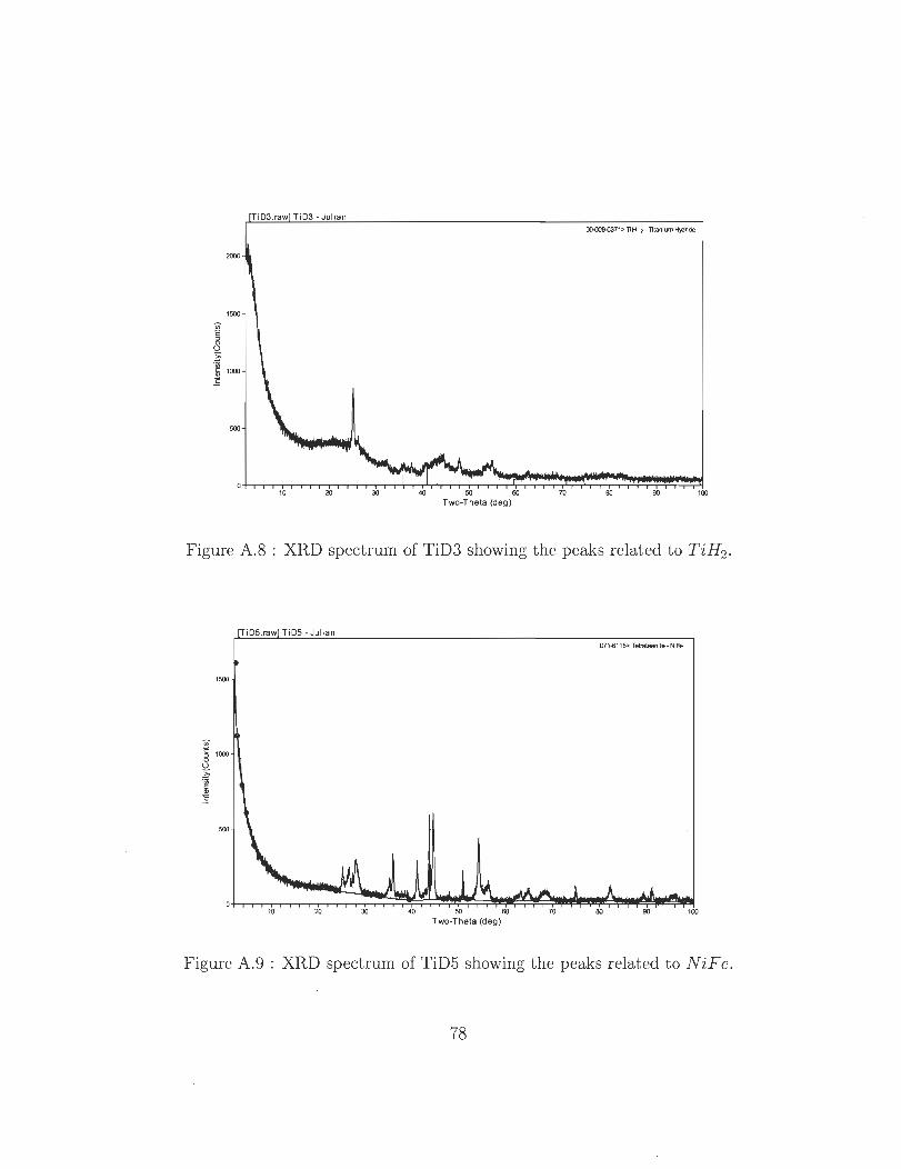
()().009...{)371> TiH 2 - Titanium ~ride
2000
1500
"' ~ "" .~ 1()()()
Ë
500
10 20 30 40 50 60 70 BD 90 100 Two-Theta (deg)
Figure A.8 XRD spectrum of TiD3 showing the peaks related to TiH2 _
1500
"' ~ 1()()()
Ü
E 'in
Iii Ë
500
10 20 30
07106116:> Tetrataenite - NiFe
40 50 60 70 BD 90 100 Two-Th eta (deg)
Figure A.9 XRD spectrum of TiD5 showing the peaks related to NiFe .
78
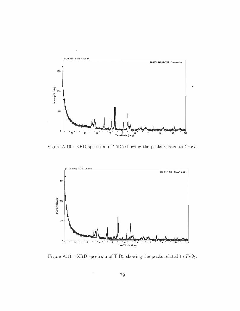
06~m5> 01.07Fe18.93 - OlIOmium Iron
1500
500
10 20 30 40 50 60 70 60 90 100
Two-Theta (deg )
Figure A.IO XRD spectrum of TiD5 showing the peaks related to Cr F e.
Q89.ô975> li02 - litanium OQde
1500
500
10 20 30 40 50 60 70 80 90 100
Two-Theta (deg )
Figure A.II XRD spectrum of TiD5 showing the peaks related to Ti02 .
79
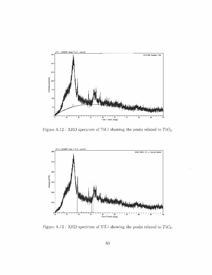
Two-Theta (deg)
Figure A.12 : XRD spectrum of TiLl showing the peaks related to Ti02 .
00-051-0622> TiC Il ·1itanium Cabide
Two-Theta (deg)
Figure A.13 : XRD spectrum of TiLl showing the peaks related to TiC8 .
80
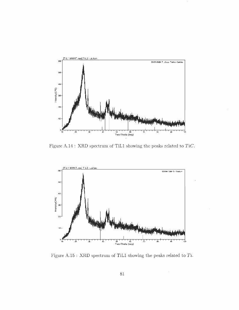
600 ()().()S1-0628> Ti 2Co.06 -Titanium Cabide
500
400
200
100
Two-The!a (deg)
Figure k 14 : XRD spectrum of TiL 1 showing the peaks related to TiC_
QO..044..1288> Ti • litanium
500
400
200
100
Two-The!a (deg)
Figure k 15 XRD speCtrum of TiLl showing the peaks related to Ti_
81
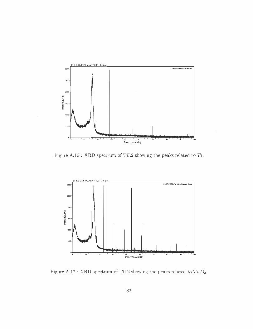
3000 ()()..()44...1288>li-Titanio.m
2500
2000
. 000
500
o~~~~~~~ .. ~~~ m m ~ c ~ ~ ro M ~ ®
Two-Theta (deg)
Figure k 16 XRD spectrum of TiL2 showing the peaks related to T i _
TiL2 CNF-PL .raw TiL2 - Julian
3000 01..071-1053> Ti A - litaritnl Oôde
2500
2000
'000
500
20 ~ 40 ~ 00 ro M ~ '00 Two-Theta (deg)
Figure A.17 XRD spectrum of TiL2 showing the peaks related to T i20 3 .
82
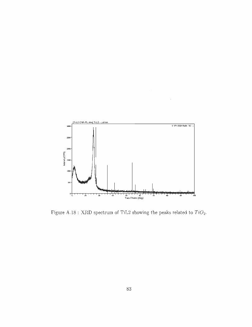
3000 OHI71~ ~Ie· TlQ 2
2500
2000
fi) 0..
~ .~ 1500
Ë
1000
500
0 10 20 30 40 50 00 70 80 00 100
Two-Thela (deg)
Figure A-18 XRD spectrum of TiL2 showing the peaks related to Ti02 -
83

Appendix B
XPS results
84
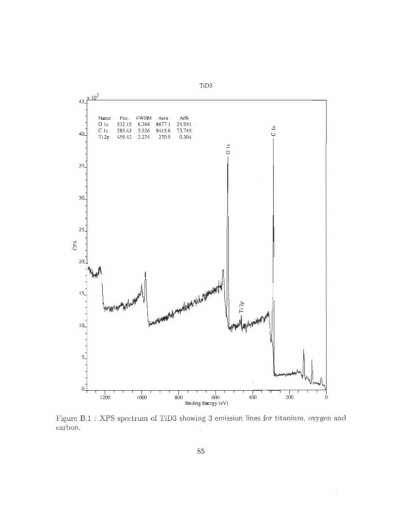
r/J Q..
U
TiD3
x 1 3 45~L----------------------------------------------------------.
40
35
30
25
20
15
JO
5
Name Ols C Is Ti2p
1200
Pos. 532.15 285.43 459.42
FWHM 6.364 3.526 2.274
1000
Area 8677.1 8415.6
270.9
At% 25.951 73.745
0.304
800 600
o
Binding Energy (eV)
0.. M
u
400 200 o
Figure B.I XPS spectrum of TiD3 showing 3 emission lines for titanium, oxygen and carbon.
85
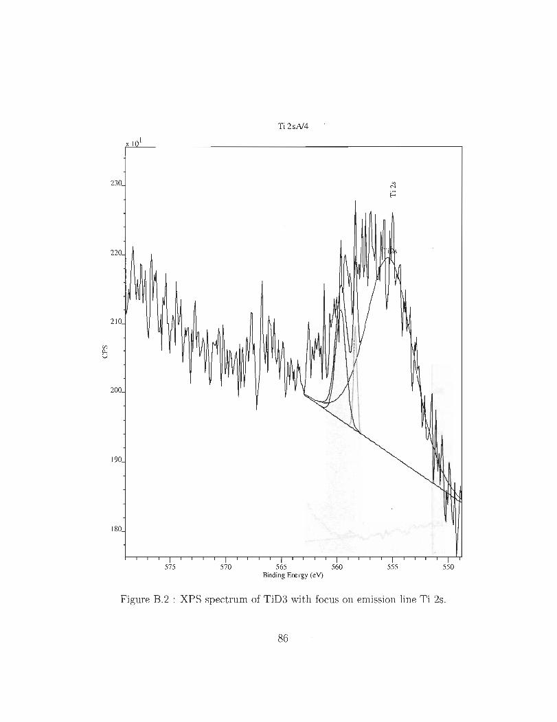
(1) Q.. U
230
220
Il ~ 210
200
190
180
1 575
~ ~ M
~
1 570
Ti2sA/4
~ ~
~ X
~ 1
565 Binding Eœrgy (eV)
1
560 1
555
"-
1 550
Figure B.2 : XPS spectrum of T iD3 with focus on emission line Ti 2s.
86
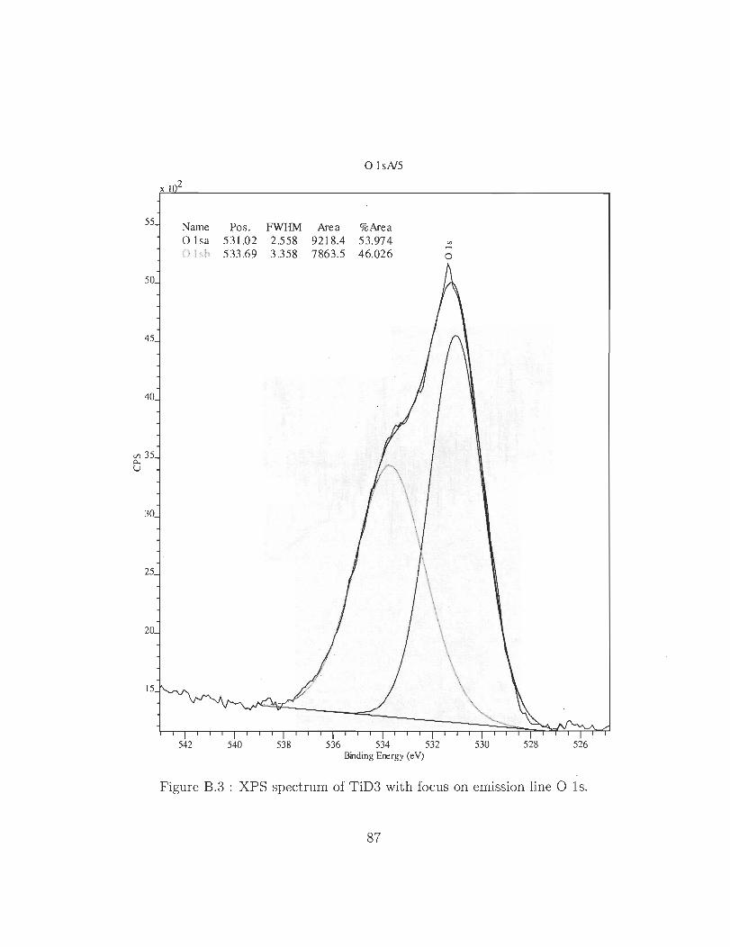
55
50
45
40
[/) 35 i:l.. u
30
25
20
15
Name 01 sa () l sb
542
Pos. FWHM 531.02 2.558 533.69 3.358
540 538
o 1sN5
Are a %Area 9218.4 53.974 7863.5 46.026
536 534 532 Binding Energy (eV)
'" ..... o
530 528 526
Figure B.3 : XPS spectrum of TiD3 with focus on emission li ne Ols.
87
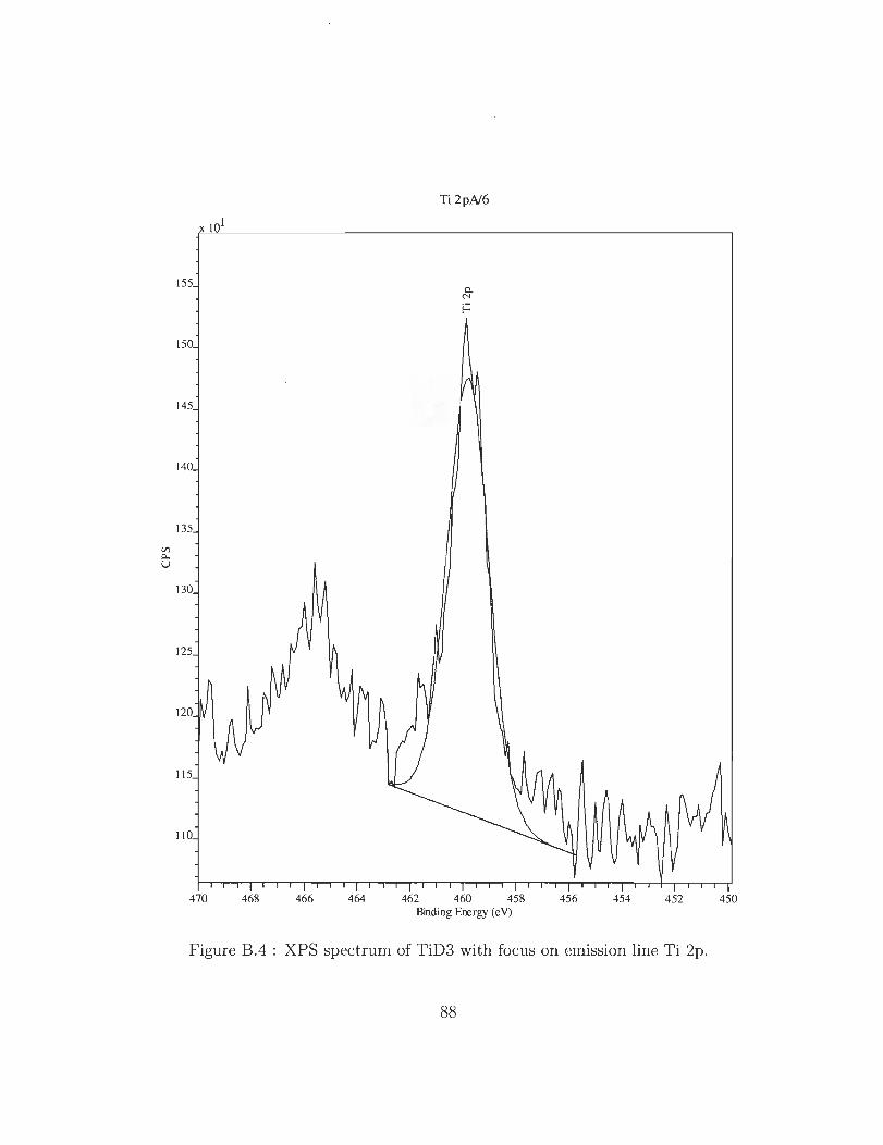
Ti 2pN6
xII
155
150
145
140
135
130
125
120
115
110
470 468 466 464 462 460 458 456 454 452 450 Binding Energy (eV)
Figure B.4 : XPS spectrum of TiD3 with focus on emission line Ti 2p.
88
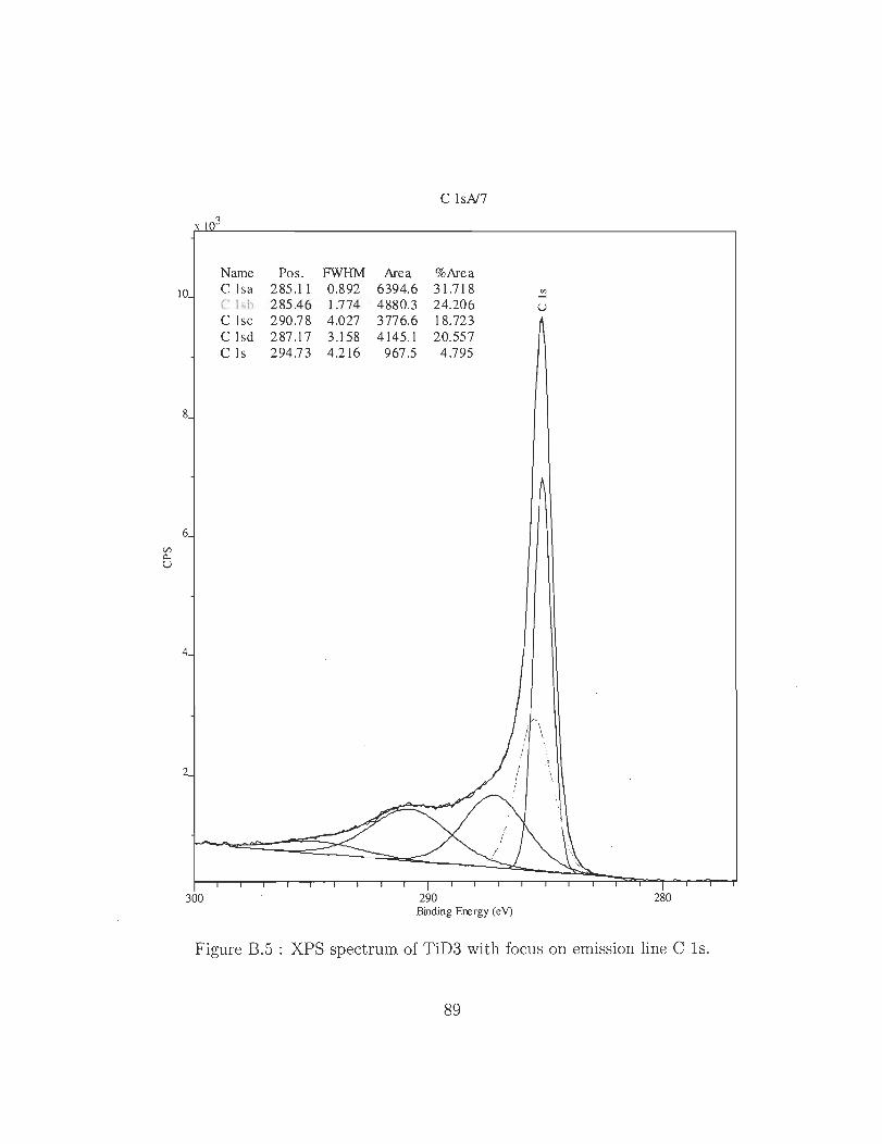
CIl 0.. U
C 1sN7
x 1 3
Name Pos. FWHM Are a %Area
10 C Isa 285.11 0.892 6394.6 31.718 ~ C lsb 285.46 1.774 4880.3 24.206 u CIse 290.78 4.027 3776.6 18.723 C lsd 287.17 3.158 4145.1 20.557 C Is 294.73 4.216 967.5 4.795
8
6
4
300 290 280 Binding Energy (eV)
Figure B.5 : XPS spectrum of TiD3 with focus on emission line C Is.
89
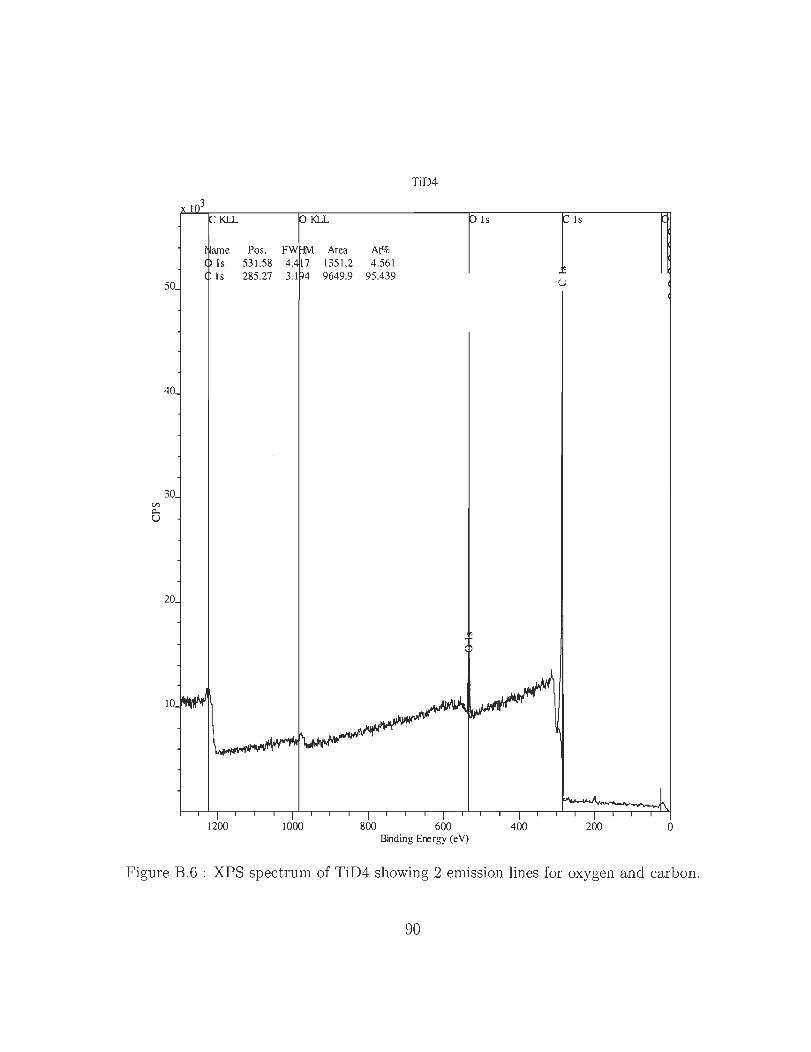
<:1) Q..;
U
50
40
30
20
10
1200
Pos. 531.58 285.27
1000
TiD4
Is Is
Area At% 1351.2 4.561 9649.9 95.439 u
800 600 400 200 o Binding Energy (eV)
Figure B.6 : XPS spectrum of TiD4 showing 2 emission lines for oxygen and carbon.
90
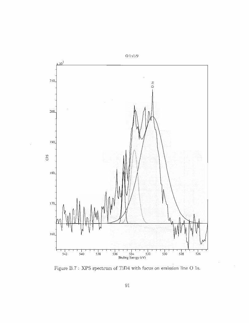
CIl 0... U
o 1s1/9
210
o
200
190
180
170
160
542 540 538 536 534 532 530 528 526 Binding Eœrgy (eV)
Figure B.7 : XPS spectrum of TiD4 with focus on emission line Ols.
91
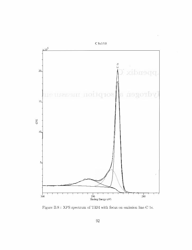
on Q.. U
C Isl/1 0
3
u 20
15
10
5
300 290 280 Binding Erergy (eV)
Figure B.8 : XPS spectrum of TiD4 with focus on emission line C ls.
92
Appendix C
Hydrogen adsorption measurements
93
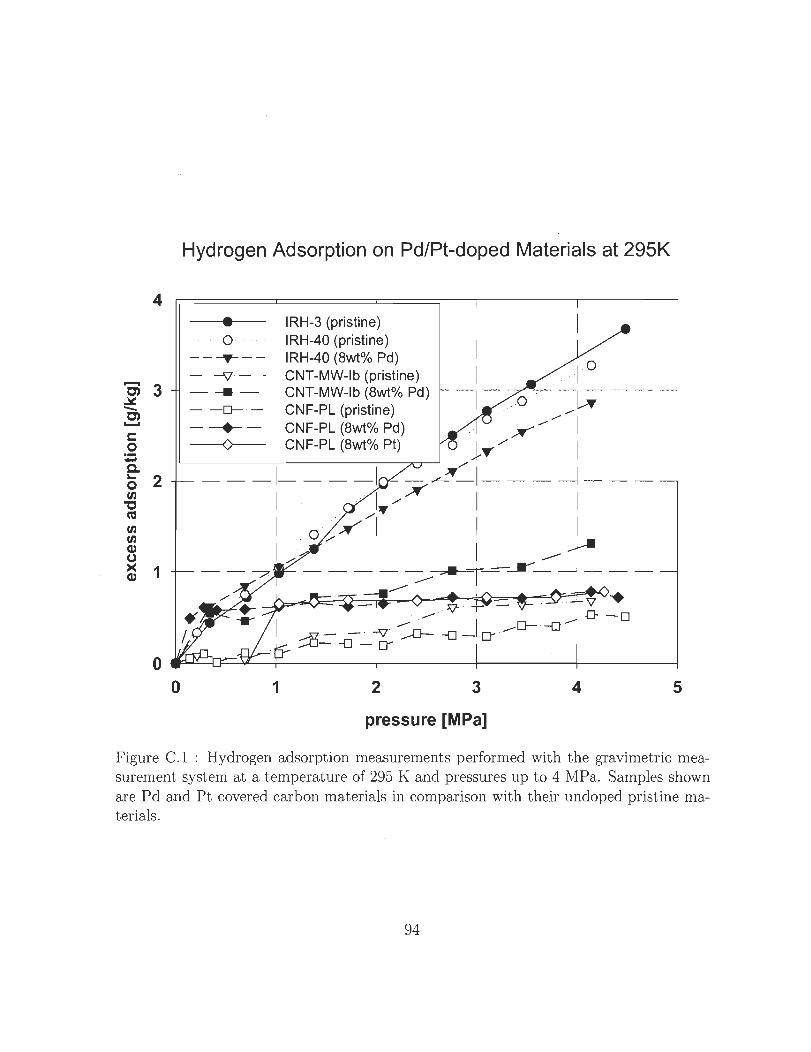
4
Hydrogen Adsorption on Pd/Pt-doped Materials at 295K
• · 0 ·
---T---
- .-v- ------ -Q- . -
--+-------0-
IRH-3 (pristine) IRH-40 (pristine) IRH-40 (8wt% Pd) CNT-MW-Ib (pristine) CNT-MW-Ib (8wt% Pd) CNF-PL (pristine) CNF-PL (8wt% Pd) CNF-PL (8wt% Pt)
1
1
1 . . ~ o - 1- .. . 0 -··· L.:T --
/
x// I o J,T'/ 1
L...-.--_-=-=--�=-=---- - -1 ------.",--_. r----'.L-"~I - __ ~ __ _ .. ··1 /.K 1 1
/'1If
1 oK 1 1 1
I ~ ' /' 1 1 ...- -r-- - --::;;r 1 - - - 1- -...- ...... T---=---.--::- , - - -
...- .. - 1 .. s:;r . D
. - -0 1 ~-- k -:.o- ~ _l o--D-~ 1 ty::-U- -a-
Icy .
o ~~~~~------~--------~-------+------~ o 1 2 3 4 5
pressure [MPa]
Figure C. I : Hydrogen adsorpt ion measurements performed with t he gravimetric measurement system at a temperature of 295 K and pressures up to 4 MPa. Samples shown are Pd and Pt covered carbon materials in comparison with their undoped pristine materials.
94
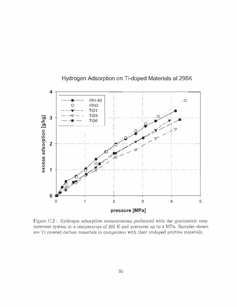
...... en ~ -en ......
Hydrogen Adsorption on Ti-doped Materials at 295K
4
• IRH-40 ..0 0 IRH3
----T- - - TiD1
3 _ . -:sv- . . TiD3 ... -_._,,-
.~~-"
-- -- -- TiD6
o œr--------~--------_r--------_+--------_.--------~
o 1 2 3 4 5
pressure [MPa]
Figure C .2 : Hydrogen adsorption measurements performed with the gravimetric measurement system at a temperature of 295 K and pressures up to 4 MPa. Samples shown are Ti covered carbon materials in comparison with their undoped pristine materials.
95
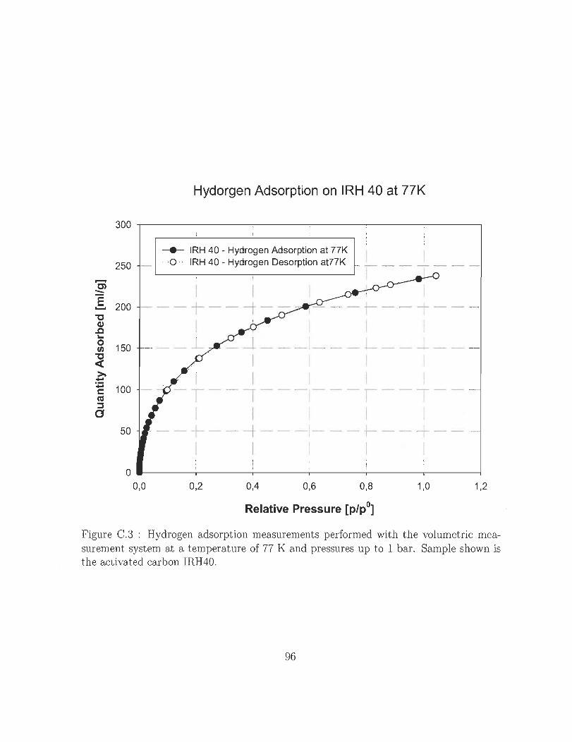
...... C) ::::
Hydorgen Adsorption on IRH 40 at 77K
300 ~------~------~------~--------~------~------~ 1
__ IRH 40 - Hydrogen Adsorption at 77K 250 - O ·· IRH 40 - Hydrogen Desorption at77K
50
1 1
--+---t---1
--- -- _ ... - 1- ... . -- -. .-1 ----- --- ---1-- .-- -1
1 1 -T--i---I---
1 1
.'-"--- --~..... --- ---.. ----r .... --- _ .. --.
1 1
--- -_. -1 -- -_._. -
---! ---
o __ ------ri ------~------+_----~r_----~------~ 0,0 0,2 0,4 0,6 0,8 1,0 1,2
Relative Pressure [pl pO]
Figure C.3 : Hydrogen adsorption measurements performed with the volumetrie measurement system at a temperature of 77 K and pressures up to 1 bar. Sample shown is the activated carbon IRH40.
96
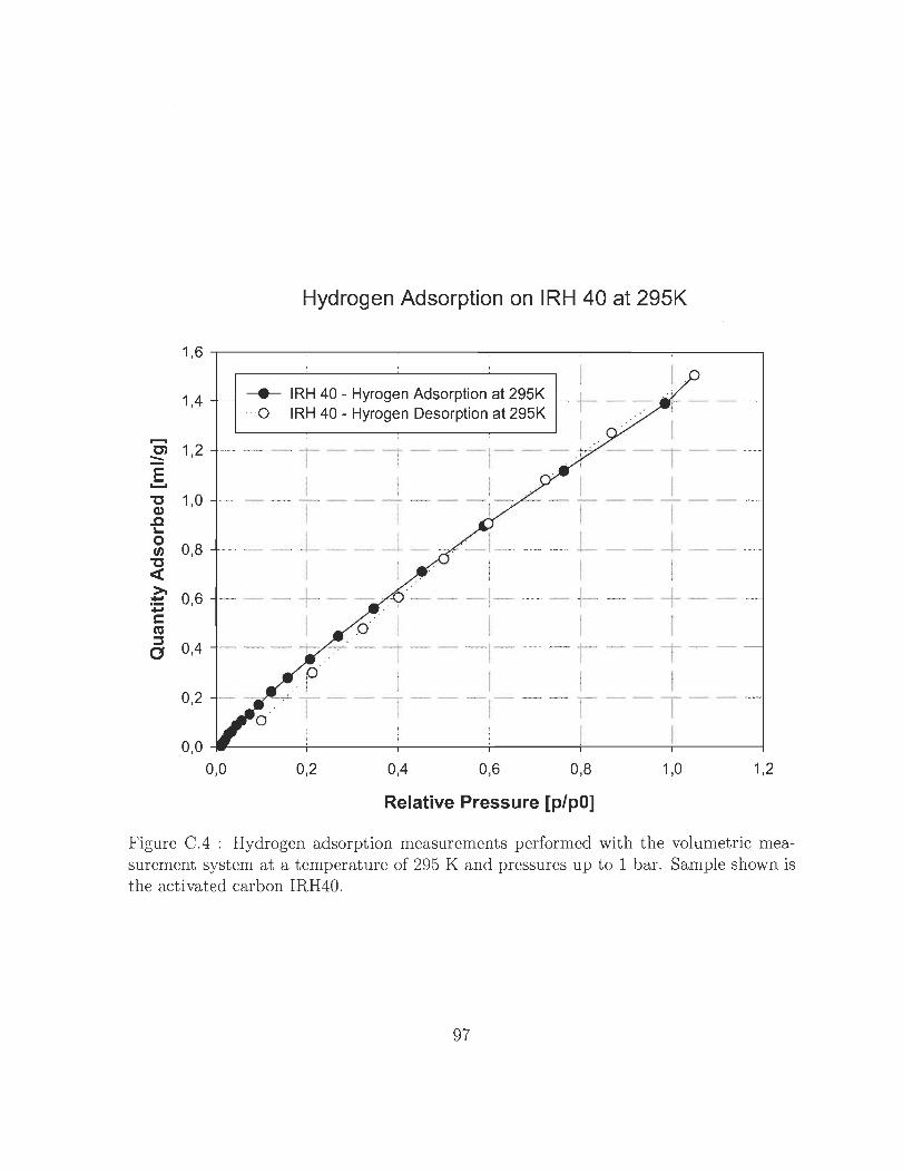
Hydrogen Adsorption on IRH 40 at 295K
1,6 ~------~--------~------~------~--------~------~
..-
1,4 --- ----- IRH 40 - Hyrogen Adsorption at 295K o IRH 40 - Hyrogen Desorption at 295K
C) 1,2 --:::: E .....
1 1 "C 1,0 - -- - -- - - - -- - - -.- - - -- -- -- ---~ ! 1 1 ~
~ 0,8 ---------.------. L---- --- -1--- --- .. _-~ 1
~ ::: 0,6 -1: ra ::::s o 0,4
0,2
_ ..... -.. _--_. ........ ........ -_ .. _. +-- ... ~.. _ .... _. 1
---\---+-I ----T' ----!
1 1
0,0 ~------_+--------r_------_r------~--------~------~
0,0 0,2 0,4 0,6 0,8 1,0 1,2
Relative Pressure [p/pO]
Figure C.4 : Hydrogen adsorption measurements performed with the volumetrie measurement system at a temperature of 295 K and pressures up to 1 bar. Sample shown is the aetivated carbon IRH40.
97
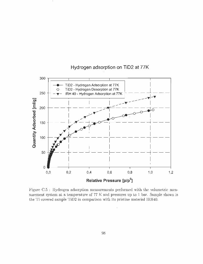
Hydrogen adsorption on TiD2 at 77K
300 ,-------,-------,-------,-------,-------,------,
250
c; :::: ..§. 200 "C CI) .c ... ~ 150
"C « ~ -:g 100 ca :1
" 50
---+-- TiD2 - Hydrogen Adsorption at 77K ·0 ·· TiD2 - Hydrogen Desorption at 77K
- .... - IRH 40 - Hydrogen Adsorption at 77K
1 1
_1 __ ~ __ _
! I_T ! --~
1 1 1 --~ t -- 1 - -1--1 - -==~ - ==-- - T --
1 )11---1---·-- 1 i 1 ---+~~ ----+-- -1---+----1----
~ 1 1
'Ji. .. . 1 1 1 j Z -l---j---j----j---I---
• 1 j 1 1 1
--+--~---l---+--~---1 1 j j 1
o --------+-------+-------+-------+-------+-----~ 0,0 0,2 0,4 0,6 0,8 1,0 1,2
Relative Pressure [pl pO]
Figure C.5 : Hydrogen adsorption measurements performed with the volumetrie measurement system at a temperature of 77 K and pressures up to 1 bar. Sample shown is the Ti eovered sample TiD2 in eomparison with its pristine material IRH40.
98
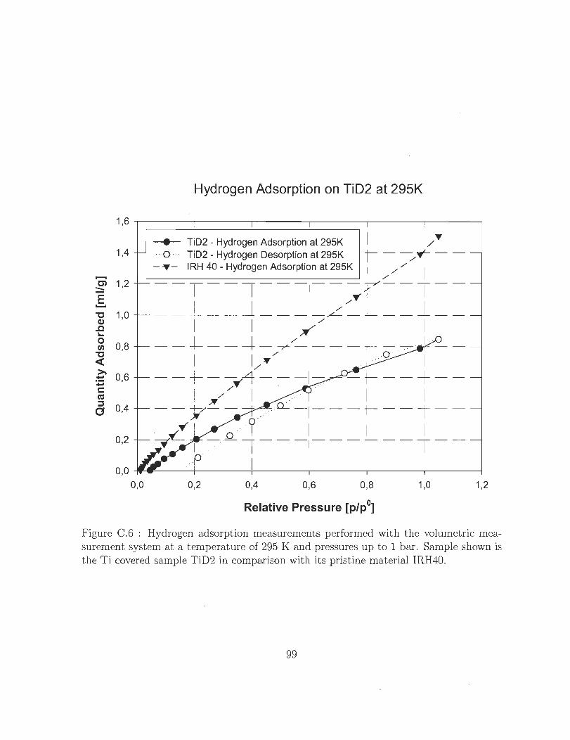
1,6
1,4
,....., Cl 1,2 :::: E ......
"'C 1 ,0 CI) .c '-0
0,8 IIJ "'C « ~
0,6 -; c: ~ :::l 0,4 a
0,2
0,0 0,0
Hydrogen Adsorption on TiD2 at 295K
_____ TiD2 - Hydrogen Adsorption at 295K 1 1/ T
··0 · TiD2 - Hydrogen Desorption at 295K 1 - - ",""1 - -'----_~_-__ I R_H_4_0_-_H_y_d_rO_g_en_A_d_s_o_rp_ti_on_at_2_9_5K---, 1 ", ", ", 1
---I---I-- -;r---I --1 1 ",'" 1 1 - - -.1_ - - - ,L-- - - - - - _ . -
1 "r'" 1 1
- - -l- - -r-/-I- - - ~ - -... . 1 "'''' 1 .
0 / -' - +- - - ...t'4 - - - 1- .
, /'" . '
1
- t---+--1 ~/ 1 . . .. 1 1 1
__ j,/- _ . CL _ 1_ - -1- - 1--.../'Y ! 0 1 1 1 1
3'T- 1 - . . . -' i ---I--- r -- T --o 1
0,2 0,4 0,6 0,8 1,0
Relative Pressure [p/pO]
1,2
Figure C .6 : Hydrogen adsorption measurements performed with the volumetrie measurement system at a temperature of 295 K and pressures up to 1 bar. Sample shown is the Ti eovered sample TiD2 in eomparison with its pristine material IRH40.
99
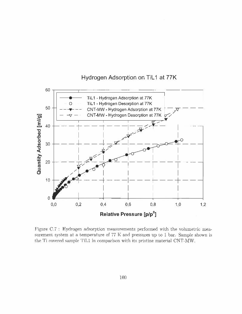
Hydrogen Adsorption on Til1 at 77K
60 ~------~------~------~--------~------~------~
...... C)
::::
50
oS 40 "C Q) .c ~
~ 30 "C ~ ~
:!:: ë 20 ca ::::s o
10
• · 0
--~--
- -v-
Til1 - Hydrogen Adsorption at 77K 1
__ 1_./1
/
Til1 - Hydrogen Desorption at 77K
CNT -MW - Hydrogen Adsorption at 77K CNT -MW - Hydrogen Desorption at 77K
1
--1- -- - T - - -t- --I- - 7 1 . . ~
1 1 1 /Jr/ 1
- - -l- - - --+ -. 5C.~I- - - h 1 4~ 1 ..
1 /.'fi~/ 1 1 1 -- ~/-?L -. . -.. ... ·- -----1 ---1 --
// 1 1 1 1 - - -t - - - 1- - - t- - - + --
1 1 1 1
0.-----1------r-----+1 ----~1------r_--~ 0,0 0,2 0,4 0,6 0,8 1,0 1,2
Relative Pressure [p/pO]
Figure C.7 : Hydrogen adsorption measurements performed with the volumetrie measurement system at a temperature of 77 K and pressures up to 1 bar. Sample shown is the Ti eovered sample TiLl in eomparison with its pristine material CNT-MW.
100
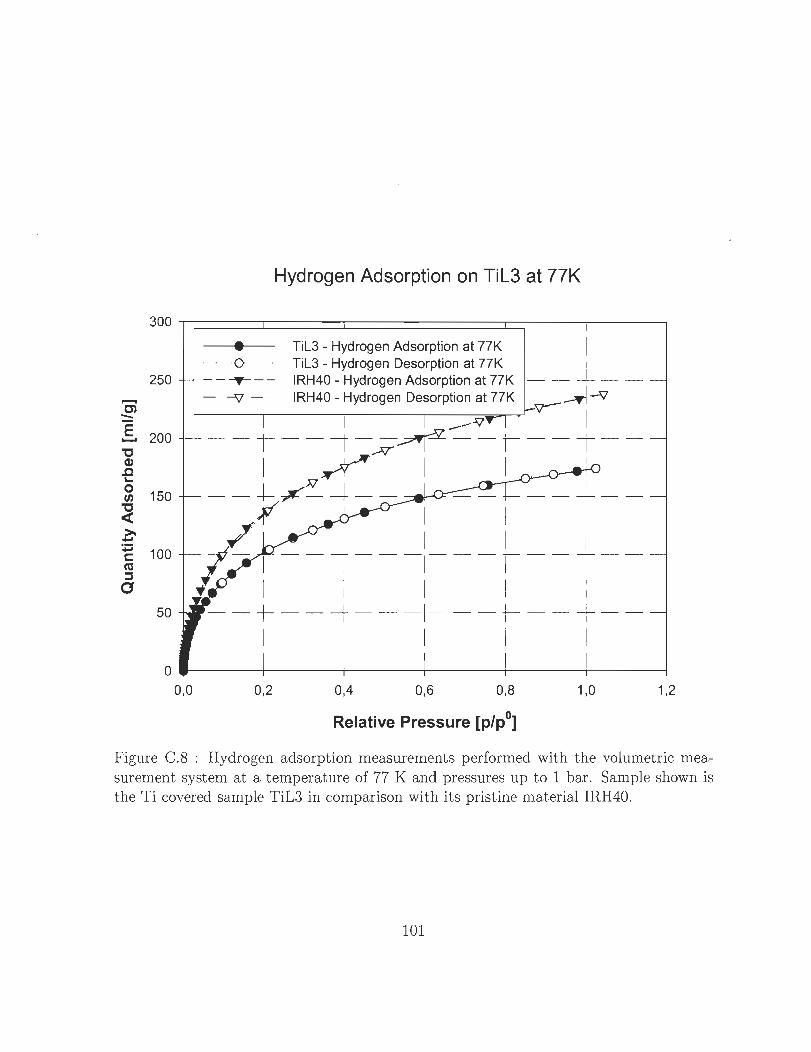
Hydrogen Adsorption on TiL3 at 77K
300~====~======~======c=======~----~~--~
...... C) ::::
250
oS 200 "C Cl) .0 ... ~ 150
~ ~ ~ 100 co ::l o
50
• TiL3 - Hydrogen Adsorption at 77K TiL3 - Hydrogen Desorption at 77K
- - -T- - - IRH40 - Hydrogen Adsorption at 77K - - - '- - -- -V _ . IRH40 - Hydrogen Desorption at 77K v--~-'V
1 1 ___ J\! 1
- - 1 - -i-..-v·.f - - ! - -1 ~ 1
1 ~~ 1 l! ---+- ",.- ---;--- _"J- ---; ---; --
/~ 1 t - 1 ---1------• 1 1 1 - - + - - -+ - - - 1- --
1 1 1
o------~-------+------~I------~------+-----~ 0,0 0,2 0,4 0,6 0,8 1,0 1,2
Relative Pressure [p/pO]
Figure C.8 : Hydrogen adsorpt ion .measurements performed wit h t he volumetrie measurement system at a temperature of 77 K and pressures up to 1 bar. Sample shown is the Ti eovered sample TiL3 in eomparison with its pristine material IRH40.
101
Bibliography
[1] PANELLA, B. HIRSCHER, M. ROTH , S. 2005. Hydrogen adsorption in different
carbon nanostructures. Stuttgart : Carbon, vol. 33
[2] YILDIRIM, T. and CIRACI, S. 2005. Titanium-Decorated Carbon anotubes
as a Potential High-Capacity Hydrogen Storage Medium. Maryland : Physical
Review Letters, vol. 94
[3] DAG, S. OZTURK, y. CIRACI, S. and YILDIRIM, T. 2005. Adsorption and
dissociation of hydrogen molecules on bare and functionalized carbon nanotubes.
Ankara: Physical Review B, vol. 72
[4] YILDIRIM, T. f - IGUEZ, J. and CIRACI, S. 2005. Molecular and dissociative
adsorption of multiple hydrogens on transition metal decorated C60 . Gaithersburg
: Physical Review B, vol. 72
[5] DAG, S. DURGUN, E. and CIRACI, S. 2004. High-conducting magnetic
nanowires obtained from uniform titanium-covered carbon nanotubes. Ankara
: Physical Review B, vol. 69
102
[6] DAG, S. CIRACI, S. 2005. Coverage and strain dependent magnetization of
titanium-coated carbon nanotubes. Ankara: Physical Review B, vol. 71
[7] ZHAO, Y. KIM, Y.-H. DILLON, A.C. HEBEN, M.J. and ZHANG, S.B. 2005.
Hydrogen Storage in Novel Organometallic Buckyballs. Colorado: Physical Re
view Letters , vol. 94
[8] KIM, Y.-H. ZHAO, Y. WILLIAMSON, A. HEBEN, M.J. and ZHANG, S.B.
2005. Non-dissociative adsorption of hydrogen molecules in light-element doped
fullerenes. Colorado : Physical Review Letters , vol. 96
[9] GALLEGO, N.C. CONTESCU, C.I. BAKER, F.S. BASOVA, Y.V. EDIE, D.D.
2006. Mechanism of Metal-Assisted Hydrogen Storage in Nanostructured Car
bons. Arlington : Annual Merit Review Meeting
[10] NOBUHARA, K. NAKANISHI, H. KASAI, H. OKIJI, A. 2000. Behaviour of
H atom in adsorption states on metal surfaces - localization and delocalization.
Osaka : Surface Science 493 271-277
[11] LACHAWIEC, A.J. GONGSHIN, Q. and YANG, R.T. 2005. Hydrogen Storage in
Nanostructured Carbons my Spillover: Bridge-Building Enhancement. Michigan
: Langmuir, vol. 21
[12] LI , L.YANG, R.T. 2005. Significantly Enhanced Hydrogen Storage in Metal
Organic Frameworks via Spillover. Michigan: JACS Communications
103
[13] LUEKING, A.D. YA G, RT. 2002. Hydrogen Spillover from a metal Oxide
Catalyst onto Carbon Nanotubes - Implications for Hydrogen Storage. Michigan
: Journal of Catalysis 206, 165-168
[14] LUEKING, A.D. YANG, RT. 2004. Hydrogen Spillover to enhance hydrogen
storage - study of the effect of carbon physicochemical properties. 2004. Pennsyl
vania: Applied Catalysis A: General 265 259-268
[15] ZHANG, y. NATHAN, W.F. CHEN, RJ. and DAI, H. 2000 Metal coating on
suspended carbon nanotubes and its implication to metal-tube interaction. Stan
ford : Chemical Physics Letters 331 35-41
[16] ZHANG, y. DAI, H. 2000. Formation of metal nanowires on suspended single
walled carbon nanotubes. Applied Physics Letters, vol. 77
[17] ZHANG, y. ZHANG, Q. LI, Y. WANG, N. ZHU, J. 2000. Coating of carbon
nanotubes with tungsten by physical vapor deposition. Beijing: Solid State
Communications, vol. 115 51-55
[18] FAN, W. GAO, L. SUN, J. 2006. Tin Oxide anoparticle-Functionalized Multi
Walled Carbon Nanotubes by the Vapor Phase Method. Shanghai: JACS, vol.
89 26712673
[19] SCHUBERT, T. WILLERT-PORADA, M. 2006. Microwave Assisted Synthesis
of Catalyst Materials for PEM Fuel Cells. Bayreuth : Advances in Microwave
and Radio Frequency Processing, Part IX
104
[20] ROUQEROL, F. ROUQUEROL, K. SING, K. 1999. Adsorption by powders and
porous solids London: Academic Press
[21] WOOD, G.O. 1992. Activated carbon adsorption capacities for vapors. Los
Alamos: Carbon 30 593-599
[22] KLUG, H.P. ALEXANDER L.E. 1974. X-Ray Diffraction Procedures: For Poly
crystalline and Amorphous Materials. John Wiley & Sons Ltd ISBN 0-471-49369-
4
[23] ALLMANN, R. KERN, A. 2002. R6ntgenpulverdiffraktometrie: Rechner
gestützte Auswertung, Phasenanalyse und Strukturbestimmung. Springer-Verlag
GmbH ISBN 3-540-43967-6
[24] WATTS, J.F. WOLSTENHOLME, J. 2003. An Introduction to Surface Analysis
by XPS and AES. John Wiley & Sons Ltd ISBN 0-470-84712-3
[25] HÜFNER, S. 2003. Photoelectron Spectroscopy Principles and Applications. 3rd
Edition Springer-Verlag Berlin Heidelberg New York ISBN 3-540-41802-4
[26] BELMABKHOUT, y. FRÈRE, M. WEIRALD, G.D. 2004. A comparative study
of the volumetric and gravimetric methods. Mons: Meas. Sci. Technol. 15 848-
858
[27] ANSON, A. BENHAM, M. JAGIELLO, J. CALLEJAS, M.A. BENITO, A.M.
MASER, W.K. ZÜTTEL, A. SUDAN, P. MARTINEZ, M.T. 2004. Hydrogen
adsorption on a single-walled carbon nanotube material: a comparative study of
three different adsorption techniques. Zaragoza: Nanotechnology 15 1503-1508
105
[28] LAN, A. MUKASYAN, A. 2005. Hydrogen Storage Capacity Characterization of
Carbon Nanotubes by a Microgravimetrical Approach. Indiana: J . Phys. Chem.
B 109
[29] KELLER, J .U. ROBENS, E. HOHENSCHE, C.d.F. Thermogravimetric and
Sorption Measurement Techniques/ Instruments. Siegen
106