universiteit antwerpen

UNIVERSITEIT ANTWERPENDepartement Wiskunde en Informatica

Academiejaar 2005-2006

Association Rule Mining met Missing Values

Michael Mampaey

Proefschrift ter verkrijging van de graad van Licentiaatin de Wetenschappen, richting Wiskunde-InformaticaPromotors:Dr. Toon CaldersDr. Bart Goethals

Acknowledgments

I would like to thank my promotors Toon Calders and Bart Goethals for theiradvice, guidance and suggestions in the process leading to the completionof this thesis.

Contents

Nederlandstalige Samenvatting i

1 Introduction 1

2 The Association Rule Model 4

2.1 Association Rules and Frequent Sets . . . . . . . . . . . . . . 42.2 Basic Concepts . . . . . . . . . . . . . . . . . . . . . . . . . . 62.3 Two Frequent Set Discovery Algorithms . . . . . . . . . . . . 8

2.3.1 Apriori . . . . . . . . . . . . . . . . . . . . . . . . . . 82.3.2 Eclat . . . . . . . . . . . . . . . . . . . . . . . . . . . . 8

2.4 Generalizations . . . . . . . . . . . . . . . . . . . . . . . . . . 9

3 Missingness 11

3.1 Classification . . . . . . . . . . . . . . . . . . . . . . . . . . . 113.1.1 MCAR - Missing completely at random . . . . . . . . 123.1.2 MAR - Missing at random . . . . . . . . . . . . . . . . 123.1.3 MNAR - Missing not at random . . . . . . . . . . . . 12

3.2 Dealing With It . . . . . . . . . . . . . . . . . . . . . . . . . . 133.2.1 Removing data . . . . . . . . . . . . . . . . . . . . . . 133.2.2 Adding data . . . . . . . . . . . . . . . . . . . . . . . 14

4 Association Rule Mining with Missing Values 15

4.1 The Problem . . . . . . . . . . . . . . . . . . . . . . . . . . . 154.2 Definitions . . . . . . . . . . . . . . . . . . . . . . . . . . . . . 16

4.2.1 Support . . . . . . . . . . . . . . . . . . . . . . . . . . 174.2.2 Confidence . . . . . . . . . . . . . . . . . . . . . . . . 174.2.3 Representativity . . . . . . . . . . . . . . . . . . . . . 174.2.4 Extensibility . . . . . . . . . . . . . . . . . . . . . . . 184.2.5 Remarks . . . . . . . . . . . . . . . . . . . . . . . . . . 18

4.3 Properties . . . . . . . . . . . . . . . . . . . . . . . . . . . . . 194.4 Frequent Set Algorithms . . . . . . . . . . . . . . . . . . . . . 20

4.4.1 Baseline algorithm . . . . . . . . . . . . . . . . . . . . 214.4.2 XMiner . . . . . . . . . . . . . . . . . . . . . . . . . . 22

4.5 Rule Generation . . . . . . . . . . . . . . . . . . . . . . . . . 24

I

5 Experimental Results 27

5.1 Sick Dataset . . . . . . . . . . . . . . . . . . . . . . . . . . . . 285.2 Eurosong Dataset . . . . . . . . . . . . . . . . . . . . . . . . . 285.3 Census Income Dataset . . . . . . . . . . . . . . . . . . . . . 30

6 Conclusions 33

II

List of Figures

2.1 The Holy Grail . . . . . . . . . . . . . . . . . . . . . . . . . . 62.2 Subset lattice over I = {a, b, c, d} . . . . . . . . . . . . . . . . 62.3 Horizontal database layout . . . . . . . . . . . . . . . . . . . 72.4 Vertical database layout . . . . . . . . . . . . . . . . . . . . . 7

3.1 Database without missing values . . . . . . . . . . . . . . . . 113.2 Database with missing values, MCAR . . . . . . . . . . . . . 123.3 Database with missing values, MAR . . . . . . . . . . . . . . 123.4 Database with missing values, MNAR . . . . . . . . . . . . . 13

4.1 Identical databases, without and with missing values . . . . . 154.2 Hierarchy of items . . . . . . . . . . . . . . . . . . . . . . . . 194.3 Subset lattice with bold frequent sets . . . . . . . . . . . . . . 194.4 Partial subtree with tail of A marked . . . . . . . . . . . . . . 23

5.1 Sick dataset experiments . . . . . . . . . . . . . . . . . . . . . 295.2 Eurosong dataset experiments . . . . . . . . . . . . . . . . . . 315.3 Census dataset experiments . . . . . . . . . . . . . . . . . . . 32

III

Nederlandstalige

Samenvatting

Missing values vormen een belangrijk en onvermijdelijk probleem in DataMining, en in data management en analyse in het algemeen. De gebruikelijketechnieken kunnen niet rechtstreeks met missingness werken, en vereisen opzijn minst een of andere vorm van pre-processing, waarbij noodgedwongenbepaalde veronderstellingen gemaakt moeten worden. In deze thesis geef ikeen effectieve oplossing voor dit probleem, evenals een efficiente implemen-tatie in een algoritme, XMiner, dat inherent association rules kan minen indatabases met missing values.

In het Association Rule Mining (ARM) model, is het doel het vindenvan alle regels van de vorm X ⇒ Y in een transactionele database D, waar-bij X en Y sets van items zijn, die intuıtief gezien, frequent voorkomenen een hoge probabiliteit hebben. Om de kwaliteit van dergelijke regelste kunnen beoordelen, bestaan er twee maten support en confidence. Demeeste ARM algoritmen kunnen in twee stappen opgedeeld worden: fre-quent set mining en rule generation. Eerst worden alle itemsets met eenhoge support gezocht, waarmee dan de association rules met hoge confi-dence gegenereerd kunnen worden. Deze laatste stap is vrij eenvoudig. Bijfrequent itemset mining wordt de exponentieel grote search space over alleitemsets doorkruist (deze vormen een subset lattice), gebruik makend vande monotoniciteitseigenschap, of de Apriori property. Deze eenvoudige maarfundamentele eigenschap zegt dat een infrequente itemset zelf geen frequentesupersets kan hebben. Dit laat toe om grote sublattices met een infre-quente itemset als root volledig te kunnen verwijderen uit de search space.Het doorkruisen van de lattice kan breadth-first of depth-first gebeuren,er bestaan vele gekende voorbeelden waaronder Apriori [2], Eclat [14] enFP-Growth [6]. Oorspronkelijk is association rule mining gedefinieerd voortransactionele databases, maar het is gemakkelijk om over te schakelen naarhet relationele database model (alhoewel dit niet geheel vanzelfsprekend is).Aangezien relationele databases meer realistisch zijn, en het probleem metmissing values er natuurlijker voorkomt, zal deze thesis ook voornamelijkhiermee werken.

i

De introductie van missing values in een database brengt vele problemenmet zich mee voor een ARM algoritme. Support en confidence worden ver-vormd, en dit kan leiden tot het verlies van goede of juist het verzinnen vanslechte regels. De oorzaak van de missingness moet hierbij beschouwd wor-den. Ontbreken er waarden volledig willekeurig? Kunnen nulls als apartewaarden behandeld worden? Kunnen er nuttige afschattingen gemaakt wor-den voor de ontbrekende waarden? De gebruikelijke aanpak is om ofwelgegevens toe te voegen, door bijvoorbeeld een gemiddelde attribuutwaardete gebruiken, ofwel tupels die nulls bevatten simpelweg te verwijderen uitde dataset. Het is duidelijk dat deze methodes de distributie van de datagrondig kunnen verstoren, wat een nefast effect kan hebben op de output.

In dit werk worden de support en confidence maten op een backwardscompatible manier geherdefinieerd, samen met een nieuwe maat representa-

tivity, die niet-missingness of waarneming uitdrukt. Deze definities komenuit voorafgaand werk door Ragel en Cremillieux [8]. De nadruk in hun werkligt op de eigenschappen en de kwaliteit van deze nieuwe definities. Ze tonenbijvoorbeeld aan dat na het willekeurig toevoegen van missing values aan eencomplete dataset, met deze nieuwe definities zo goed als alle oorspronkelijkassociation rules teruggevonden kunnen worden. Er wordt echter geen aan-dacht besteed aan een efficiente implementatie, wat noodzakelijk is vanwegede eigenschappen van deze nieuwe maten.

De nieuwe support, die wel adequaat is, is echter niet meer monotoon.Dit maakt het onmogelijk om hem te gebruiken bij het doorkruisen van desubset lattice, zoals met de oorspronkelijke definitie wel gedaan kon worden.Hiertoe introduceer ik extensibility, een nieuwe eigenschap voor itemsets.Existensibility is verwant met het frequent zijn van een itemset (en metzijn representativiteit), maar is monotoon, wat het bruikbaar maakt bij hetdoorkruisen van de subset lattice. Het XMiner algoritme (eXtensible itemsetMiner), dat gebaseerd is op het Eclat algoritme wordt gepresenteerd, en aande hand van experimenten wordt aangetoond dat het effectief en efficientwerkt, door het te vergelijken met een baseline-algoritme.

Hierdoor hebben we echter slechts nog maar een frequent set miningalgoritme, terwijl association rule mining natuurlijk het genereren van regelsvereist (hoewel frequent set mining op zich ook al interessant kan zijn).Spijtig genoeg, net zoals support niet meer monotoon is, kunnen regels nietmeer zo vanzelfsprekend gegenereerd worden uit de frequente itemsets. Hetkan zelfs nodig zijn om de support van infrequente sets te moeten berekenenom de confidence van een aanverwante association rule te kennen. DoorXMiner zo aan te passen dat deze itemsets, die wel noodzakelijk zijn naastde echte frequente itemsets, allemaal gevonden worden, (maar zonder devolledige subset lattice te doorkruisen!), kan er gegarandeerd worden dat dittoch vrij goed, albeit niet optimaal verwezenlijkt kan worden. Zodra dit isbereikt, is het genereren van association rules opnieuw een eenvoudige zaak.

ii

Chapter 1

Introduction

Missing values comprise an important and unavoidable problem in DataMining, and in data management and analysis in general. Conventionalmining techniques are not capable of working with missingness directly, andrequire some form of (likely biased) workaround or preprocessing at the least.In this work I provide an effective theoretical solution, as well as an efficientalgorithm, XMiner, for inherently mining association rules in databases withmissing values.

In the Association Rule Mining (ARM) model [1], the goal is to find allrules of the form X ⇒ Y in a transactional database D, with X and Y setsof items, that intuitively, occur frequently and have a high probability. Toassess the goodness of such rules, two measures for association rules are de-fined, support and confidence. Typically, association rule mining algorithmscan be divided into two parts: frequent set mining and rule generation, i.e.,first all itemsets with high support are found, from which all confident rulesare then generated. The latter step is rather straightforward. For frequentset mining, the subset lattice over all items spanning the exponentially largesearch space of itemsets, is traversed using the monotonicity of the supportmeasure. This simple yet fundamental property states that no superset ofan infrequent itemset, can itself be frequent. This allows large sublatticeswith an infrequent set as root to be pruned completely. The traversal can bebreadth- or depth-first; many algorithms exists, the most famous ones beingApriori [2], Eclat [14] and FP-Growth [6]. While association rule miningis conventionally defined for the transactional database model, it is easily(though not entirely trivially) extended to and implemented for relationaldatabases. Since these databases are more real-world, and the problem ofmissing data occurs more naturally there, this work will deal with the rela-tional model instead.

The introduction of missing data in the input database brings manyproblems for an ARM algorithm. The support and confidence measuresbecome distorted, which could result in the loss of good or fabrication of bad

1

rules. The actual cause of missingness, the missingness mechanism, mustbe considered. Are the values missing at random? Can nulls be treated asa separate value? Can useful estimations of the missing values be made?The usual approach is to either impute the missing data e.g. by using amean attribute value, or to remove tuples with nulls. It is clear that thesetechniques can severely distort the distribution of the data, which can havea bad result on the output.

In this work the support and confidence measures are redefined in a back-wards compatible manner (extended if you will), along with a newly definedmeasure representativity, which expresses non-missingness or observation.These definitions derive from previous work by Ragel and Cremillieux [8].The emphasis in their work is on the properties and good applicability ofthese measures. For example, they show that after randomly inserting nullsin a complete database, most if not all original association rules can still beretrieved. Unfortunately they do not focus on the implementation of theirextended measures, which is a necessity due to some of the properties of themeasures.

The new support measure, though adequate, no longer exhibits themonotonicity property. This makes it impossible to be used as a subset lat-tice traversal guide, as was the case with the regular definition of support.Therefore I introduce extensibility, a new itemset property. Extensibility isrelated to the support of an itemset (as well as its representativity), but itis monotone and hence this property will aid traversal of the search space.The XMiner algorithm (for eXtensible itemset Miner), based on the Eclatalgorithm (and with some elements which are similar to the MaxMiner algo-rithm), is given and through experimentation it is shown to be effective andefficient, by being compared against a straightforward baseline algorithm.

This leaves us however with only an itemset mining algorithm, whereasassociation rule mining of course requires the generation of actual rulesfrom them (although itemsets in themselves can also be interesting). Un-fortunately, just as the extended support measure was no longer monotone,the extended confidence measure causes trouble as well. The cause of thislies with the straightforwardness of rule generation from frequent itemsets,which it is anything but now. Indeed, it might even be so that the supportcount of an itemset that is infrequent, is required to compute the confidenceof an association rule. By adapting XMiner in such a way that the itemsets,necessary not only for frequent set mining but for rule generation too, areall found (yet without traversing the entire search space!), it is ensured thatthis can be accomplished fairly well, albeit not optimally. Once this hasbeen achieved, rule generation is again a straightforward matter.

The next chapter reviews basic frequent itemset mining and associationrule mining, chapter 3 explains some missingness mechanisms and techniquesthat are commonly in use to try to deal with missingness. Chapter 4 thengives the definitions and properties of the extended itemset and association

2

rule measures, and supplies the algorithms that provide efficient implemen-tation. Experimental results are listed in chapter 5, chapter 6 concludes thisthesis.

3

Chapter 2

The Association Rule Model

This chapter briefly reviews Association Rule Mining. The first section dis-cusses Frequent Set Mining. Then, section two covers basic concepts. Sec-tion three describes the algorithms Apriori and Eclat. Section four toucheson some generalizations.

2.1 Association Rules and Frequent Sets

Association rule mining was introduced by Agrawal et al. [1]. Due to moderntechnologies, it is possible for organizations to acquire and store lots of data,finding useful and unexpected patterns in this data can be an interesting butcomplex task. A typical example used is that of a supermarket database,which contains information about customer transactions, such as customer,date, products purchased, price, etc. Analysis of this data can be usefulto the store for making marketing decisions such as pricing strategies orproduct placement in the store. The process of finding useful informationin such databases is called market basket analysis.

Staying with our supermarket example, we are interested in findinggroups of products (items) that are frequently purchased together, andassociations between these products, such as “beer and chips are boughttogether” or “if a customer buys beer, he also buys chips”. As an associ-ation rule this would be: “beer” ⇒ “chips”. Of course we only want therules that are useful to us, so we define measures for these rules to ex-press their relevance. First of all, if only a few customers bought “beer”and “chips” together, the set of items {“beer”, “chips”} will have no sta-tistical significance. So we set a minimum support threshold, to excludethese itemsets. When we know that “beer” and “chips” are frequent, wecan construct rules with them. The rule “beer” ⇒ “chips” expresses theconditional probability between the itemsets {“beer”} and {“chips”}. Thestrength of this rule is called the confidence, e.g. a confidence of 80% meansthat Pr(“chips”|“beer”)=80% i.e. “80% of all customers who bought beer,

4

also bought chips”. Again we can set a threshold, to eliminate those rulesthat are not confident. Both measures are necessary, in that no one impliesthe other.

Formally, we are given a database D of transactions, where each transac-tion t contains a number of items from a finite item universe I. A set I ⊆ Iis called an itemset, an itemset with cardinality k is called a k-itemset. Thefrequency (or count) of an itemset I is defined to be the number of trans-actions t in D that support I, i.e. the transactions that have I as a subset.An association rule is a conditional implication of the form X ⇒ Y , whereX and Y are itemsets for which X 6= φ, Y 6= φ and X ∩ Y = φ.

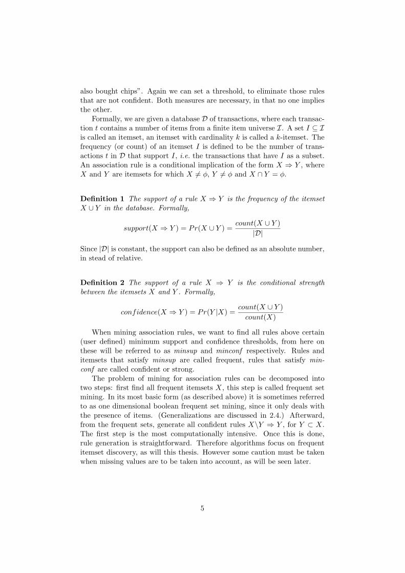
Definition 1 The support of a rule X ⇒ Y is the frequency of the itemset

X ∪ Y in the database. Formally,

support(X ⇒ Y ) = Pr(X ∪ Y ) =count(X ∪ Y )

|D|

Since |D| is constant, the support can also be defined as an absolute number,in stead of relative.

Definition 2 The support of a rule X ⇒ Y is the conditional strength

between the itemsets X and Y . Formally,

confidence(X ⇒ Y ) = Pr(Y |X) =count(X ∪ Y )

count(X)

When mining association rules, we want to find all rules above certain(user defined) minimum support and confidence thresholds, from here onthese will be referred to as minsup and minconf respectively. Rules anditemsets that satisfy minsup are called frequent, rules that satisfy min-

conf are called confident or strong.The problem of mining for association rules can be decomposed into

two steps: first find all frequent itemsets X, this step is called frequent setmining. In its most basic form (as described above) it is sometimes referredto as one dimensional boolean frequent set mining, since it only deals withthe presence of items. (Generalizations are discussed in 2.4.) Afterward,from the frequent sets, generate all confident rules X\Y ⇒ Y , for Y ⊂ X.The first step is the most computationally intensive. Once this is done,rule generation is straightforward. Therefore algorithms focus on frequentitemset discovery, as will this thesis. However some caution must be takenwhen missing values are to be taken into account, as will be seen later.

5

2.2 Basic Concepts

The single most important property used in frequent set mining algorithms,is the monotonicity principle, aka the Apriori property. It simply statesthat the support of a superset Y of X, must always be equal or less thanthe support of X. From this we infer that all subsets of a frequent itemsetmust also be frequent, or alternatively, no superset of an infrequent itemsetcan be frequent.

X ⊂ Y ⇒ supp(X) ≥ supp(Y )

Figure 2.1: The Holy Grail

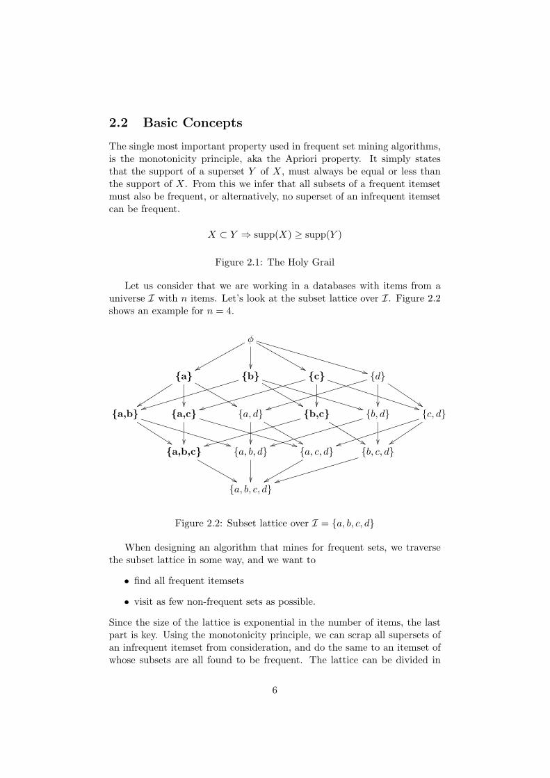
Let us consider that we are working in a databases with items from auniverse I with n items. Let’s look at the subset lattice over I. Figure 2.2shows an example for n = 4.

φ

xxqqqqqqqqqqqqq

²² &&MMMMMMMMMMMMM

**VVVVVVVVVVVVVVVVVVVVVVVVVV

{a}

yytttttttttt

²² &&MMMMMMMMMMM{b}

ttiiiiiiiiiiiiiiiiiiiiiii

&&MMMMMMMMMMM

**VVVVVVVVVVVVVVVVVVVVVVV {c}

tthhhhhhhhhhhhhhhhhhhhhhhh

²²**UUUUUUUUUUUUUUUUUUUUU {d}

ttiiiiiiiiiiiiiiiiiiiiiiii

²² $$JJJJJJJJJ

{a,b}

%%JJJJJJJJJ

**UUUUUUUUUUUUUUUUUUUUU {a,c}

²² **VVVVVVVVVVVVVVVVVVVVVV {a, d}

²² &&MMMMMMMMMM{b,c}

tthhhhhhhhhhhhhhhhhhhhhh

%%KKKKKKKKKK{b, d}

ttiiiiiiiiiiiiiiiiiiiiii

²²

{c, d}

ttiiiiiiiiiiiiiiiiiii

zzttttttttt

{a,b,c}

&&MMMMMMMMMM{a, b, d}

²²

{a, c, d}

xxqqqqqqqqqq{b, c, d}

ttiiiiiiiiiiiiiiiiiiii

{a, b, c, d}

Figure 2.2: Subset lattice over I = {a, b, c, d}

When designing an algorithm that mines for frequent sets, we traversethe subset lattice in some way, and we want to

• find all frequent itemsets

• visit as few non-frequent sets as possible.

Since the size of the lattice is exponential in the number of items, the lastpart is key. Using the monotonicity principle, we can scrap all supersets ofan infrequent itemset from consideration, and do the same to an itemset ofwhose subsets are all found to be frequent. The lattice can be divided in

6

two parts by a frequency border. As illustrated in figure 2.2, the itemsets inbold are frequent, the other ones are not. Many lattice traversal strategiescan be employed, usually a breadth-first (the most famous being Apriori) ordepth-first (such as Eclat or FP-Growth) technique is used, although otherpossibilities exist such as best-first by some heuristic.

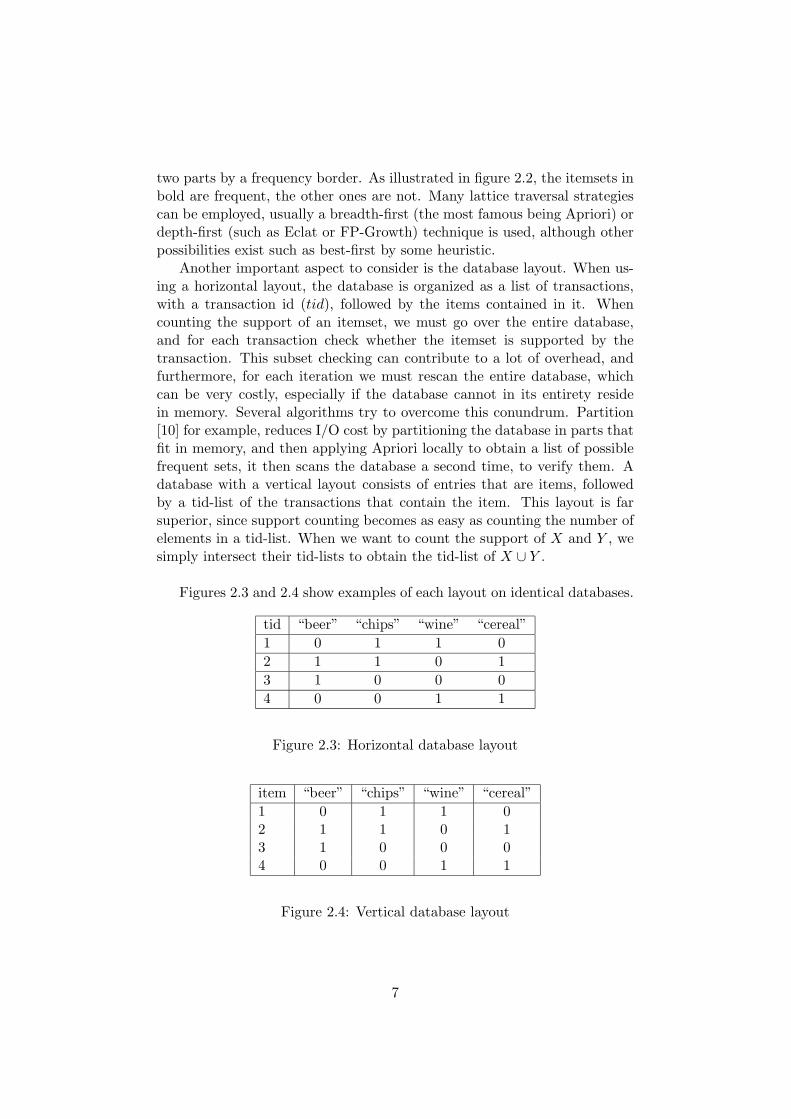
Another important aspect to consider is the database layout. When us-ing a horizontal layout, the database is organized as a list of transactions,with a transaction id (tid), followed by the items contained in it. Whencounting the support of an itemset, we must go over the entire database,and for each transaction check whether the itemset is supported by thetransaction. This subset checking can contribute to a lot of overhead, andfurthermore, for each iteration we must rescan the entire database, whichcan be very costly, especially if the database cannot in its entirety residein memory. Several algorithms try to overcome this conundrum. Partition[10] for example, reduces I/O cost by partitioning the database in parts thatfit in memory, and then applying Apriori locally to obtain a list of possiblefrequent sets, it then scans the database a second time, to verify them. Adatabase with a vertical layout consists of entries that are items, followedby a tid-list of the transactions that contain the item. This layout is farsuperior, since support counting becomes as easy as counting the number ofelements in a tid-list. When we want to count the support of X and Y , wesimply intersect their tid-lists to obtain the tid-list of X ∪ Y .

Figures 2.3 and 2.4 show examples of each layout on identical databases.

tid “beer” “chips” “wine” “cereal”

1 0 1 1 0

2 1 1 0 1

3 1 0 0 0

4 0 0 1 1

Figure 2.3: Horizontal database layout

item “beer” “chips” “wine” “cereal”

1 0 1 1 02 1 1 0 13 1 0 0 04 0 0 1 1

Figure 2.4: Vertical database layout

7

2.3 Two Frequent Set Discovery Algorithms

In this section we will describe two of the best known algorithms for dis-covering boolean frequent itemsets. They are Apriori and Eclat. Extensiveand detailed descriptions can be found in (among others) [3] [13]. Manyvariations and specialized optimizations for these algorithms exist.

2.3.1 Apriori

The Apriori algorithm was introduced by Agrawal et al. [3]. It employs abreadth-first, generate-and-test strategy on the search space.

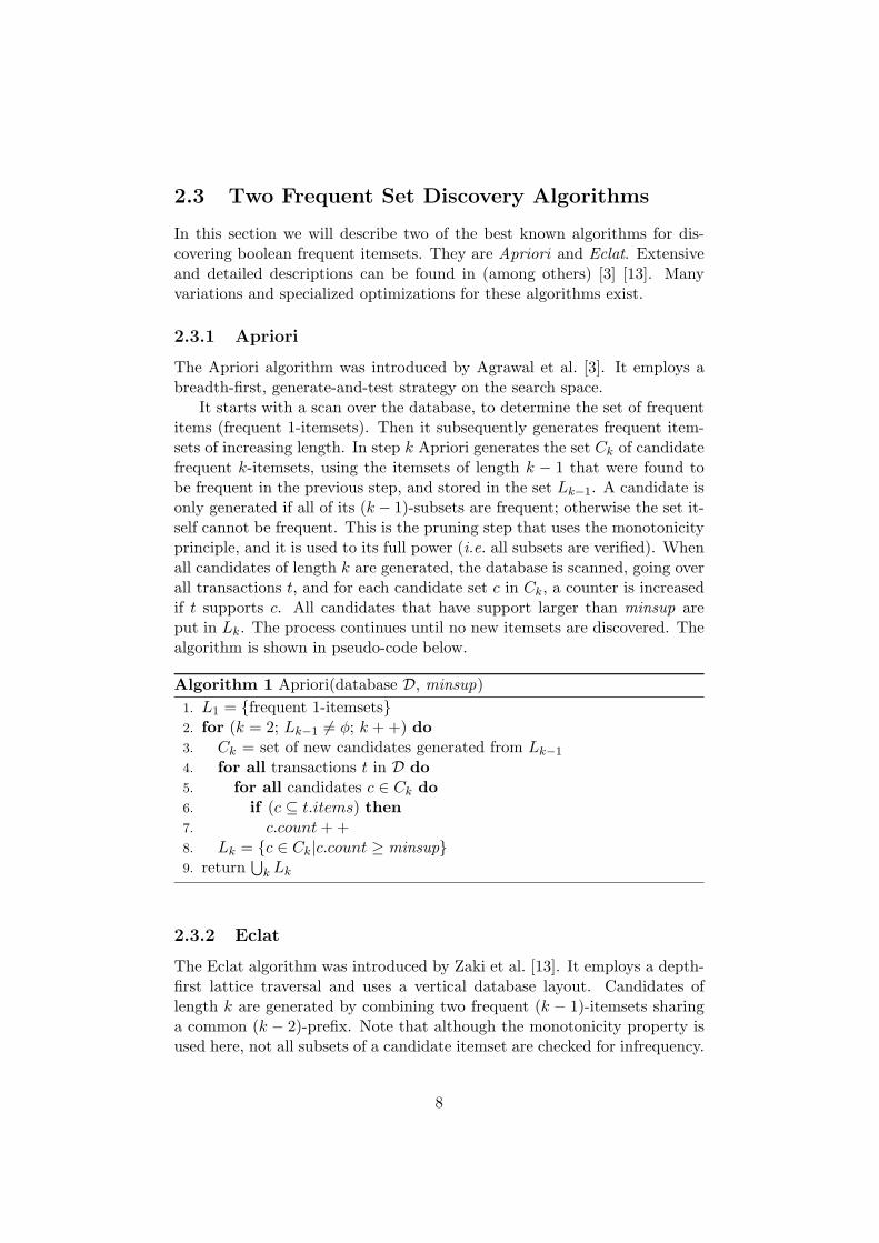
It starts with a scan over the database, to determine the set of frequentitems (frequent 1-itemsets). Then it subsequently generates frequent item-sets of increasing length. In step k Apriori generates the set Ck of candidatefrequent k-itemsets, using the itemsets of length k − 1 that were found tobe frequent in the previous step, and stored in the set Lk−1. A candidate isonly generated if all of its (k − 1)-subsets are frequent; otherwise the set it-self cannot be frequent. This is the pruning step that uses the monotonicityprinciple, and it is used to its full power (i.e. all subsets are verified). Whenall candidates of length k are generated, the database is scanned, going overall transactions t, and for each candidate set c in Ck, a counter is increasedif t supports c. All candidates that have support larger than minsup areput in Lk. The process continues until no new itemsets are discovered. Thealgorithm is shown in pseudo-code below.

Algorithm 1 Apriori(database D, minsup)

1. L1 = {frequent 1-itemsets}2. for (k = 2; Lk−1 6= φ; k + +) do

3. Ck = set of new candidates generated from Lk−1

4. for all transactions t in D do

5. for all candidates c ∈ Ck do

6. if (c ⊆ t.items) then

7. c.count + +8. Lk = {c ∈ Ck|c.count ≥ minsup}9. return

⋃

k Lk

2.3.2 Eclat

The Eclat algorithm was introduced by Zaki et al. [13]. It employs a depth-first lattice traversal and uses a vertical database layout. Candidates oflength k are generated by combining two frequent (k − 1)-itemsets sharinga common (k − 2)-prefix. Note that although the monotonicity property isused here, not all subsets of a candidate itemset are checked for infrequency.

8

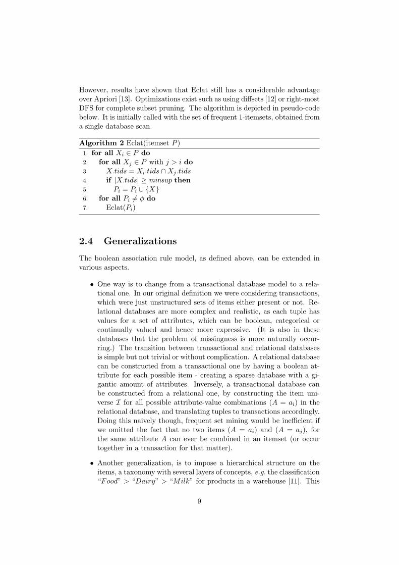
However, results have shown that Eclat still has a considerable advantageover Apriori [13]. Optimizations exist such as using diffsets [12] or right-mostDFS for complete subset pruning. The algorithm is depicted in pseudo-codebelow. It is initially called with the set of frequent 1-itemsets, obtained froma single database scan.

Algorithm 2 Eclat(itemset P )

1. for all Xi ∈ P do

2. for all Xj ∈ P with j > i do

3. X.tids = Xi.tids ∩ Xj .tids4. if |X.tids| ≥ minsup then

5. Pi = Pi ∪ {X}6. for all Pi 6= φ do

7. Eclat(Pi)

2.4 Generalizations

The boolean association rule model, as defined above, can be extended invarious aspects.

• One way is to change from a transactional database model to a rela-tional one. In our original definition we were considering transactions,which were just unstructured sets of items either present or not. Re-lational databases are more complex and realistic, as each tuple hasvalues for a set of attributes, which can be boolean, categorical orcontinually valued and hence more expressive. (It is also in thesedatabases that the problem of missingness is more naturally occur-ring.) The transition between transactional and relational databasesis simple but not trivial or without complication. A relational databasecan be constructed from a transactional one by having a boolean at-tribute for each possible item - creating a sparse database with a gi-gantic amount of attributes. Inversely, a transactional database canbe constructed from a relational one, by constructing the item uni-verse I for all possible attribute-value combinations (A = ai) in therelational database, and translating tuples to transactions accordingly.Doing this naively though, frequent set mining would be inefficient ifwe omitted the fact that no two items (A = ai) and (A = aj), forthe same attribute A can ever be combined in an itemset (or occurtogether in a transaction for that matter).

• Another generalization, is to impose a hierarchical structure on theitems, a taxonomy with several layers of concepts, e.g. the classification“Food” > “Dairy” > “Milk” for products in a warehouse [11]. This

9

might be useful to mine very broad rules such as “Dairy”⇒“Fruit”,whereas too specific rules such as “Skim milk” ⇒ “Pine apple” arenot frequent enough to be detected. This generalization itself canbe expanded as well by also allowing cross-level rules, or maintainingdifferent support thresholds at different concept levels.

• Sometimes it is not necessary to mine all frequent sets, but we areonly interested in maximal frequent itemsets. A frequent itemset I iscalled maximal if none of its supersets is frequent. For example, therule “Bread” ⇒ “Milk” “Eggs” contains the rule “Bread” ⇒ “Milk”completely, and hence the latter is superfluous. From the set of allmaximal frequent itemsets we can infer all frequent sets, by generat-ing their subsets (however we can not derive their supports). Notethat the maximal frequent itemsets alone completely describe the fre-quency border in the subset lattice. It has been shown that by usingpruning techniques for this specific situation, maximal set mining canbe accomplished efficiently, i.e. linearly in the number of maximal fre-quent sets, whereas the number of all frequent sets can be exponentialin the length of the longest (maximal) itemset [4].

10

Chapter 3

Missingness

This chapter will give an overview of different missingness mechanisms, andcommon techniques for dealing with the missing value problem.

Missing data occurs in many real-world datasets. Because of it the com-plexity of analysis increases, and the results can be influenced considerably.Ideally, we would want to make the same inferences about the data, as ifwe had the complete dataset (if this is possible at all). A key componenthere is the mechanism at which this missingness occurs, i.e. the probabilityof a value being missing, depending either on other attributes, or its ownvalue. Hence, when analyzing a dataset with missing values, we must takethe missingness mechanism into account. Unfortunately, this mechanism isnot always known, and assumptions about the data must be made.

3.1 Classification

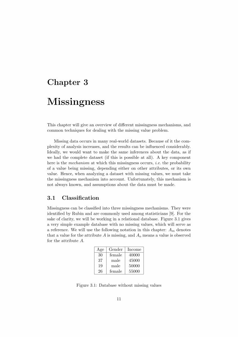
Missingness can be classified into three missingness mechanisms. They wereidentified by Rubin and are commonly used among statisticians [9]. For thesake of clarity, we will be working in a relational database. Figure 3.1 givesa very simple example database with no missing values, which will serve asa reference. We will use the following notation in this chapter: Am denotesthat a value for the attribute A is missing, and Ao means a value is observedfor the attribute A.

Age Gender Income

30 female 4000037 male 4500019 male 5000026 female 55000

Figure 3.1: Database without missing values

11

3.1.1 MCAR - Missing completely at random

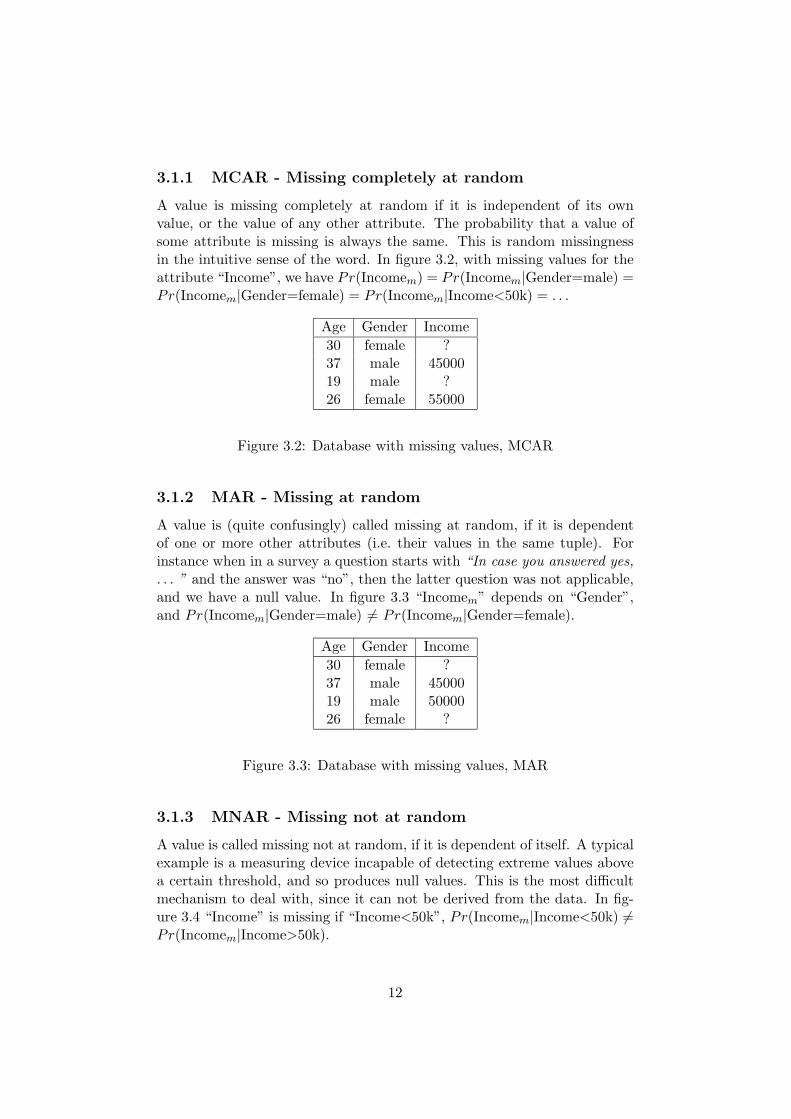
A value is missing completely at random if it is independent of its ownvalue, or the value of any other attribute. The probability that a value ofsome attribute is missing is always the same. This is random missingnessin the intuitive sense of the word. In figure 3.2, with missing values for theattribute “Income”, we have Pr(Incomem) = Pr(Incomem|Gender=male) =Pr(Incomem|Gender=female) = Pr(Incomem|Income<50k) = . . .

Age Gender Income

30 female ?37 male 4500019 male ?26 female 55000

Figure 3.2: Database with missing values, MCAR

3.1.2 MAR - Missing at random

A value is (quite confusingly) called missing at random, if it is dependentof one or more other attributes (i.e. their values in the same tuple). Forinstance when in a survey a question starts with “In case you answered yes,

. . . ” and the answer was “no”, then the latter question was not applicable,and we have a null value. In figure 3.3 “Incomem” depends on “Gender”,and Pr(Incomem|Gender=male) 6= Pr(Incomem|Gender=female).

Age Gender Income

30 female ?37 male 4500019 male 5000026 female ?

Figure 3.3: Database with missing values, MAR

3.1.3 MNAR - Missing not at random

A value is called missing not at random, if it is dependent of itself. A typicalexample is a measuring device incapable of detecting extreme values abovea certain threshold, and so produces null values. This is the most difficultmechanism to deal with, since it can not be derived from the data. In fig-ure 3.4 “Income” is missing if “Income<50k”, Pr(Incomem|Income<50k) 6=Pr(Incomem|Income>50k).

12

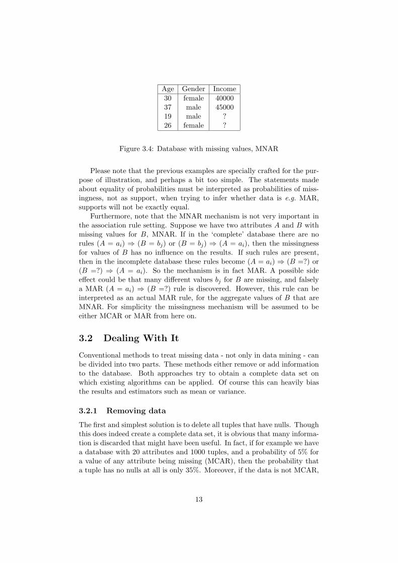
Age Gender Income

30 female 4000037 male 4500019 male ?26 female ?

Figure 3.4: Database with missing values, MNAR

Please note that the previous examples are specially crafted for the pur-pose of illustration, and perhaps a bit too simple. The statements madeabout equality of probabilities must be interpreted as probabilities of miss-ingness, not as support, when trying to infer whether data is e.g. MAR,supports will not be exactly equal.

Furthermore, note that the MNAR mechanism is not very important inthe association rule setting. Suppose we have two attributes A and B withmissing values for B, MNAR. If in the ‘complete’ database there are norules (A = ai) ⇒ (B = bj) or (B = bj) ⇒ (A = ai), then the missingnessfor values of B has no influence on the results. If such rules are present,then in the incomplete database these rules become (A = ai) ⇒ (B =?) or(B =?) ⇒ (A = ai). So the mechanism is in fact MAR. A possible sideeffect could be that many different values bj for B are missing, and falselya MAR (A = ai) ⇒ (B =?) rule is discovered. However, this rule can beinterpreted as an actual MAR rule, for the aggregate values of B that areMNAR. For simplicity the missingness mechanism will be assumed to beeither MCAR or MAR from here on.

3.2 Dealing With It

Conventional methods to treat missing data - not only in data mining - canbe divided into two parts. These methods either remove or add informationto the database. Both approaches try to obtain a complete data set onwhich existing algorithms can be applied. Of course this can heavily biasthe results and estimators such as mean or variance.

3.2.1 Removing data

The first and simplest solution is to delete all tuples that have nulls. Thoughthis does indeed create a complete data set, it is obvious that many informa-tion is discarded that might have been useful. In fact, if for example we havea database with 20 attributes and 1000 tuples, and a probability of 5% fora value of any attribute being missing (MCAR), then the probability thata tuple has no nulls at all is only 35%. Moreover, if the data is not MCAR,

13

then the results will become skewed, and estimators such as mean will be-come biased, since more tuples with a certain value for a certain attributewill be removed. A similar deletion technique is removing all attributes thathave missing data, but this is even more ridiculous.

3.2.2 Adding data

The second alternative to obtain a complete database is to fill in the gaps.Several techniques exist, some of the most common are listed below.

Mean and mode imputation

With mean imputation, all nulls for a given attribute are replaced by themean of all observed values for that attribute. While for attributes withvery few missing values that are MCAR this might not be too bad, it is clearthat when many values are missing, or they are not MCAR, this severelydeforms the data. For one, standard deviation will be underestimated. Ofcourse this technique is only applicable to continuously valued attributes,not categorical. Mode imputation is more (only) applicable to categoricalattributes, it replaces the nulls for an attribute with the most observedvalue for that attribute. Similar remarks as with mean imputation applyhere, especially variance will be lowered.

The missingness category

Another possibility is to add an extra category that represents the missing-ness for an attribute. Clearly if the missingness mechanism is not MAR,(and even then), it is possible that very dissimilar groups of attributes be-come grouped under this new category.

Multiple imputation

Rather than filling up the dataset once to obtain a complete dataset, anotherpossibility consists of creating several complete datasets, each with differentvalues for the missingness imputed. Each of these datasets can then beanalyzed separately, after which the means and variance of all of these resultsare used to obtain the final results. Although multiple imputation can yieldresults that are far better than the previous methods, it is clear that it iscomputationally more expensive, and that any derived inferences from thistechnique are still only valid within some acceptability interval.

14

Chapter 4

Association Rule Mining

with Missing Values

This chapter describes the problem of missing values for association rulemining, extends and defines some new itemset and association rule mea-sures, along with some theoretical properties, and implements them in analgorithm with several possible optimizations.

4.1 The Problem

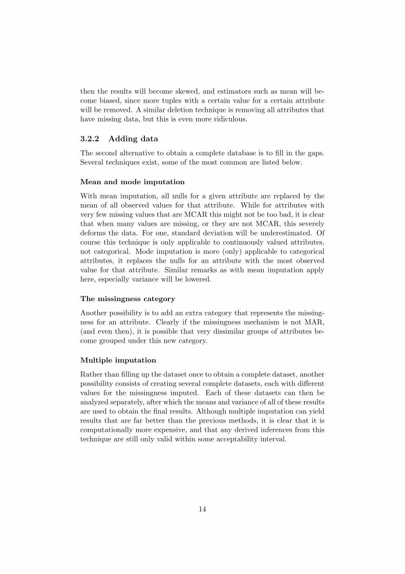
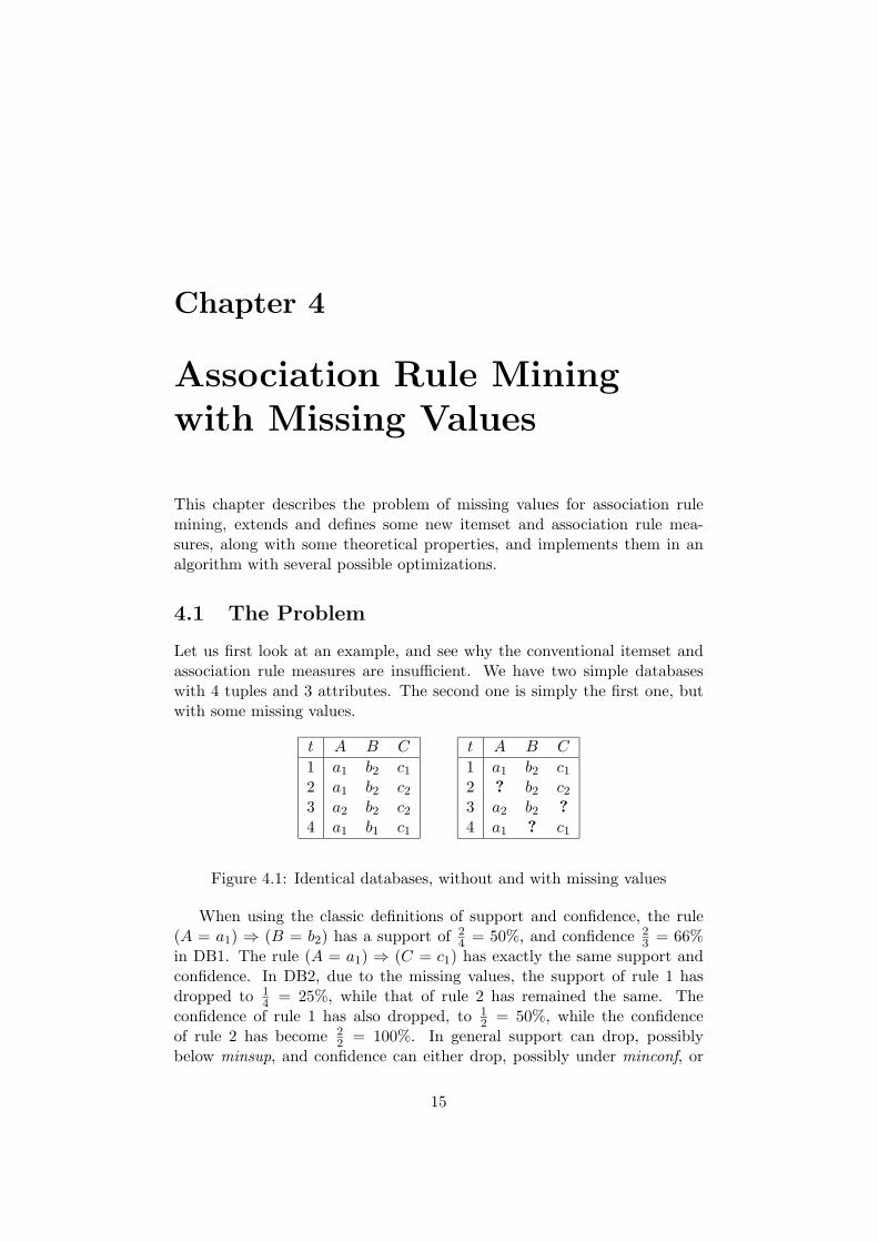
Let us first look at an example, and see why the conventional itemset andassociation rule measures are insufficient. We have two simple databaseswith 4 tuples and 3 attributes. The second one is simply the first one, butwith some missing values.

t A B C

1 a1 b2 c1

2 a1 b2 c2

3 a2 b2 c2

4 a1 b1 c1

t A B C

1 a1 b2 c1

2 ? b2 c2

3 a2 b2 ?

4 a1 ? c1

Figure 4.1: Identical databases, without and with missing values

When using the classic definitions of support and confidence, the rule(A = a1) ⇒ (B = b2) has a support of 2

4= 50%, and confidence 2

3= 66%

in DB1. The rule (A = a1) ⇒ (C = c1) has exactly the same support andconfidence. In DB2, due to the missing values, the support of rule 1 hasdropped to 1

4= 25%, while that of rule 2 has remained the same. The

confidence of rule 1 has also dropped, to 1

2= 50%, while the confidence

of rule 2 has become 2

2= 100%. In general support can drop, possibly

below minsup, and confidence can either drop, possibly under minconf, or

15

rise, making a rule over-confident. This is because we no longer take intoaccount the transactions with missing values, while it might be possible thatthe ? hides a value that is useful. The reason for this distortion is that werecognize the missing values as some value that is never equal to the one weare counting. We completely ignore the special meaning of the ?’s - theymay or may not hide a value of interest to us, we just don’t know.

4.2 Definitions

To solve this problem, some new and extended itemset and association rulemeasures need to be introduced. They take into account the possibility ofmissing values, and treat them accordingly. These quite straightforwardmeasures were defined by Ragel and Cremillieux [8], who in their work ap-plied them to find rules in a database with missing values inserted at random.By inspecting the results, it was shown that most, if not all of the originalrules could be retrieved, and almost no new (false) rules were introduced.However, no mention of algorithmic implementation is made, except thata version of Apriori was used. Also, the third measure (representativity,which will prove to be key), never even seems to be used after being defined.I assume that a traditional frequent set mining algorithm was used, andpost-processing was applied on the results. Here I will formally (re)definethe measures, and explain them.

First, let us lay down some notation. We are working in a relationaldatabase D (which as seen earlier, can be viewed as a transactional database).Each tuple has a transaction/tuple identifier tid. Attributes A, B, C, . . . andtheir values a, b, c, . . . will be written in uppercase and lowercase respectively.An item is an attribute value pair, written as (A = ai). The missingness

item is written as (A =?), indicating a missing value for the attribute A.(Note that although this item’s notation is similar to that of a proper item,mindlessly treating it as such is wrong.) Also, we have the attribute item

(A = ∗), which is used when a value (any value) is observed for the attributeA. (The same remark as for the missingness item applies).

Itemsets are sets of these pairs, in general they can also contain miss-ingness and attribute items. This generality allows us to mine interestingrules that carry information about the missingness mechanisms present inthe database. However, this extension is not inherently more difficult, so Iwill not focus on it here. The only tricky part lies with the double role thatattribute items play (due to the upcoming definitions), but through care-ful implementation this is quite manageable. Furthermore, we will assumethat itemsets are consistent, in that no two items with the same attribute(e.g. (A = a1) and (A = a2), or (B = b1) and (B =?)) can be in an itemsettogether. The only trivial exception to this is e.g. (C = c1) and (C = ∗),but since the latter is implied by the former, it can be omitted.

16

By the count of an itemset, we mean the absolute number of transactionsin D that support that itemset:

Definition 3 count(X) := |{t ∈ D|X ⊆ t.items}|

Finally, the attribute set of an itemset X is defined as:

Definition 4 X∗ := {(A = ∗)|(A = ai) ∈ X}

For example, {(A = a1), (B = b2), (C = ∗), (D =?)}∗ = {(A = ∗), (B = ∗)}.

4.2.1 Support

When looking at what went wrong in example 4.1, we see that we countedall tuples that support X, and divided it by the total number of tuples |D|.However, some of those tuples have missing values for some attributes of X.Since the ?’s may or may not hide complete transactions that support X,we should omit these tuples. Only the tuples that have no missing values forany of the attributes in X∗ will be considered - although those tuples mightstill have missing values for other attributes! Statistically this is expressedby Pr(X|X∗). We can now define the new support measure:

Definition 5

supp(X) :=count(X)

count(X∗)

4.2.2 Confidence

A similar observation can be made for the confidence of an association rule.For the rule X ⇒ Y there might be missing values for the antecedent Y .The solution here is to again only consider those tuples that do not havemissing values for Y . Statistically this is expressed by Pr(Y |X ∪ Y ∗).

Definition 6

conf(X ⇒ Y ) :=count(X ∪ Y )

count(X ∪ Y ∗)

4.2.3 Representativity

Apart from confidence and support, representativity is introduced as a newmeasure. The rationale behind it is to limit the influence of itemsets thatare scarcely observed (i.e. many tuples in D have missing values for someof the attributes of the itemset), on confidence and support. In other wordsthe sample of D that has no missing values for the attribute set of X mustbe a representative sample.

Definition 7

rep(X) :=count(X∗)

|D|

17

4.2.4 Extensibility

One more definition is due, I define the extensibility property of an itemset(which is not a measure). Later we will see why this is much needed.

Definition 8 An itemset X is called extensible, if an itemset Y exists such

that X ∪ Y is frequent and representative, i.e.

∃Y :

{

supp(X ∪ Y ) ≥ minsup

rep(X ∪ Y ) ≥ minrep

Note that Y may be the empty set, so all itemsets that are frequent andrepresentative are trivially extensible. Furthermore, it goes without sayingthat extensibility is monotone.

4.2.5 Remarks

• Because of the new definition of confidence, we can no longer easilyconstruct the confident rules from the frequent sets. Before, the con-fidence of a rule X ⇒ Y was equal to supp(X ∪ Y )/supp(X). This isnot true anymore, since

supp(X ∪ Y )

supp(X)=

count(X ∪ Y )/count(X∗ ∪ Y ∗)

count(X)/count(X∗).

Statistically Pr(Y |X ∪ Y ∗) only equals Pr(Y |X) if X and Y are in-dependent.

• As was the case with the classic support definition, representativity isdefined relative to |D|. In the following however representativity canbe either relative or absolute depending on the context.

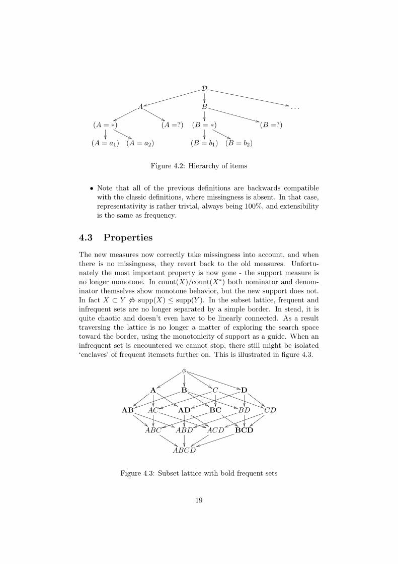
• Looking closely at the definition of representativity, it is very reminis-cent of another definition: the conventional definition of support. Ina way, representativity can be considered to be support on the level ofmissingness, or rather, observation. The following equality illustratesthis (since for any X, (X∗)∗ = φ):

rep(X) =count(X∗)

count((X∗)∗).

This implies a hierarchy among different kinds of items or itemsets,as shown in figure 4.2. A single attribute A has two children (A = ∗)and (A =?). The former still has more specific children, namely theattribute-value pairs (A = ai). Implementing the new definitions in ageneralized itemset mining algorithm (which has already been studiedextensively [11]) is not possible, since the generalized monotonicityprinciple does not hold, i.e. the support of more general itemsets isnot necessarily higher than the support of more specific itemsets.

18

D

tthhhhhhhhhhhhhhhhhh

²²,,YYYYYYYYYYYYYYYYYYYYYYYYY

A

wwpppppppp

&&MMMMMMMM B

²² ++VVVVVVVVVVVVVVVV . . .

(A = ∗)

²² ''NNNNNNN(A =?) (B = ∗)

²² ''NNNNNNN(B =?)

(A = a1) (A = a2) (B = b1) (B = b2)

Figure 4.2: Hierarchy of items

• Note that all of the previous definitions are backwards compatiblewith the classic definitions, where missingness is absent. In that case,representativity is rather trivial, always being 100%, and extensibilityis the same as frequency.

4.3 Properties

The new measures now correctly take missingness into account, and whenthere is no missingness, they revert back to the old measures. Unfortu-nately the most important property is now gone - the support measure isno longer monotone. In count(X)/count(X∗) both nominator and denom-inator themselves show monotone behavior, but the new support does not.In fact X ⊂ Y 6⇔ supp(X) ≤ supp(Y ). In the subset lattice, frequent andinfrequent sets are no longer separated by a simple border. In stead, it isquite chaotic and doesn’t even have to be linearly connected. As a resulttraversing the lattice is no longer a matter of exploring the search spacetoward the border, using the monotonicity of support as a guide. When aninfrequent set is encountered we cannot stop, there still might be isolated‘enclaves’ of frequent itemsets further on. This is illustrated in figure 4.3.

φ

yyttttttttt

²²%%KKKKKKKKK

**TTTTTTTTTTTTTTTTT

A

||xxxx

xxx

²² %%JJJJJJJJ B

uujjjjjjjjjjjjjjj

%%KKKKKKKK

**TTTTTTTTTTTTTTTT C

ttiiiiiiiiiiiiiiiii

²²))SSSSSSSSSSSSSSS D

ttjjjjjjjjjjjjjjjj

²² ##FF

FFFF

F

AB

""FF

FFFF

))TTTTTTTTTTTTT AC

²² **UUUUUUUUUUUUUUU AD

²² %%KKKK

KKK

BC

ttiiiiiiiiiiiiiii

$$IIIIIIBD

ttjjjjjjjjjjjjjj

²²

CD

uukkkkkkkkkkkkk

{{xxxx

xx

ABC

%%JJJJ

JJJ

ABD

²²

ACD

yytttt

ttt

BCD

ttjjjjjjjjjjjj

ABCD

Figure 4.3: Subset lattice with bold frequent sets

19

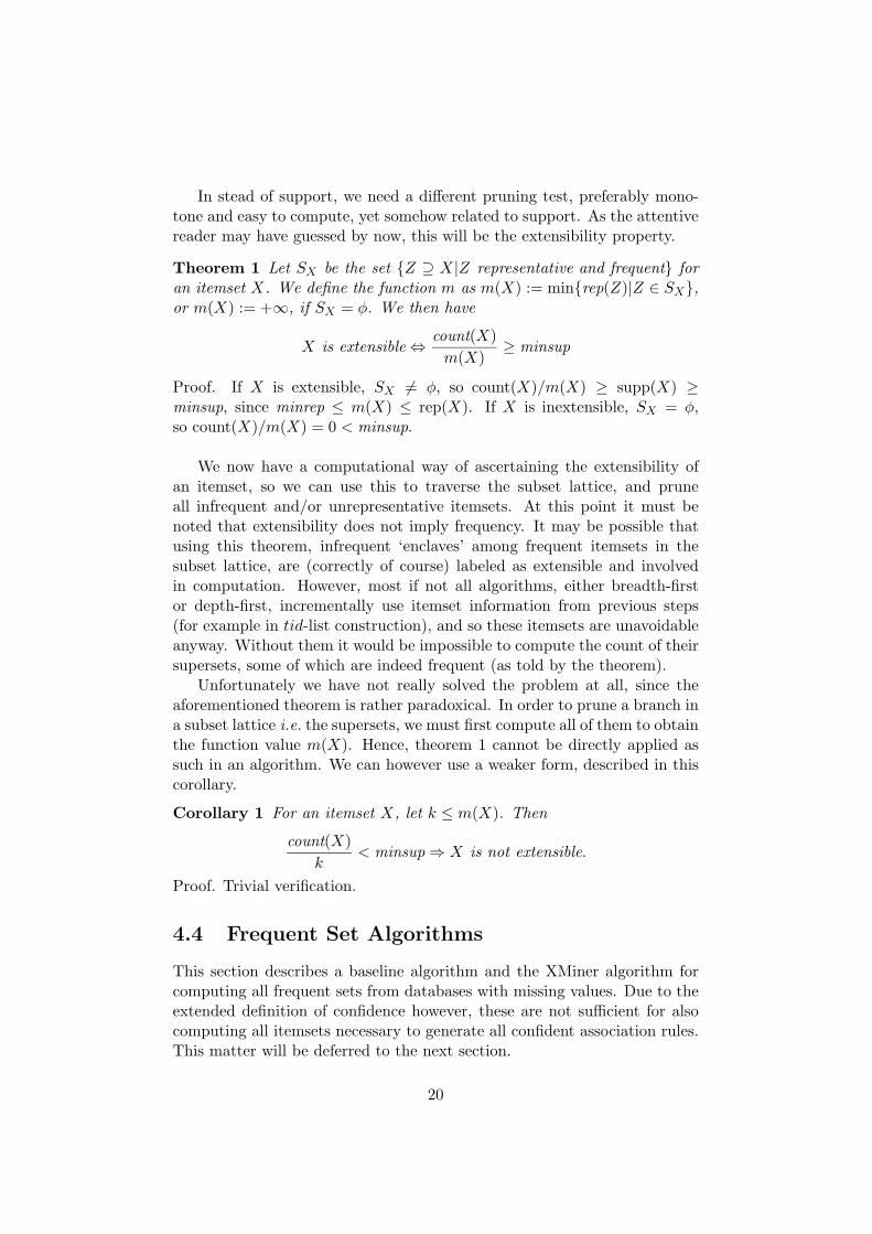
In stead of support, we need a different pruning test, preferably mono-tone and easy to compute, yet somehow related to support. As the attentivereader may have guessed by now, this will be the extensibility property.

Theorem 1 Let SX be the set {Z ⊇ X|Z representative and frequent} for

an itemset X. We define the function m as m(X) := min{rep(Z)|Z ∈ SX},or m(X) := +∞, if SX = φ. We then have

X is extensible ⇔count(X)

m(X)≥ minsup

Proof. If X is extensible, SX 6= φ, so count(X)/m(X) ≥ supp(X) ≥minsup, since minrep ≤ m(X) ≤ rep(X). If X is inextensible, SX = φ,so count(X)/m(X) = 0 < minsup.

We now have a computational way of ascertaining the extensibility ofan itemset, so we can use this to traverse the subset lattice, and pruneall infrequent and/or unrepresentative itemsets. At this point it must benoted that extensibility does not imply frequency. It may be possible thatusing this theorem, infrequent ‘enclaves’ among frequent itemsets in thesubset lattice, are (correctly of course) labeled as extensible and involvedin computation. However, most if not all algorithms, either breadth-firstor depth-first, incrementally use itemset information from previous steps(for example in tid-list construction), and so these itemsets are unavoidableanyway. Without them it would be impossible to compute the count of theirsupersets, some of which are indeed frequent (as told by the theorem).

Unfortunately we have not really solved the problem at all, since theaforementioned theorem is rather paradoxical. In order to prune a branch ina subset lattice i.e. the supersets, we must first compute all of them to obtainthe function value m(X). Hence, theorem 1 cannot be directly applied assuch in an algorithm. We can however use a weaker form, described in thiscorollary.

Corollary 1 For an itemset X, let k ≤ m(X). Then

count(X)

k< minsup ⇒ X is not extensible.

Proof. Trivial verification.

4.4 Frequent Set Algorithms

This section describes a baseline algorithm and the XMiner algorithm forcomputing all frequent sets from databases with missing values. Due to theextended definition of confidence however, these are not sufficient for alsocomputing all itemsets necessary to generate all confident association rules.This matter will be deferred to the next section.

20

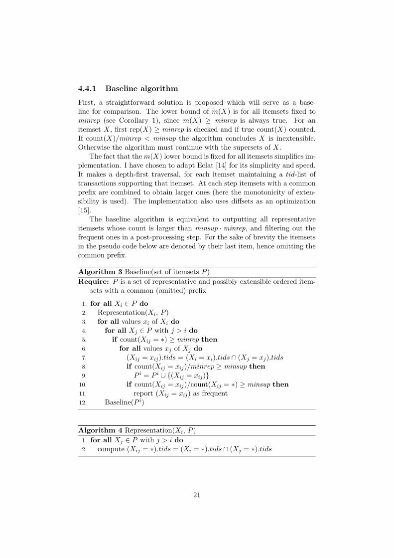
4.4.1 Baseline algorithm

First, a straightforward solution is proposed which will serve as a base-line for comparison. The lower bound of m(X) is for all itemsets fixed tominrep (see Corollary 1), since m(X) ≥ minrep is always true. For anitemset X, first rep(X) ≥ minrep is checked and if true count(X) counted.If count(X)/minrep < minsup the algorithm concludes X is inextensible.Otherwise the algorithm must continue with the supersets of X.

The fact that the m(X) lower bound is fixed for all itemsets simplifies im-plementation. I have chosen to adapt Eclat [14] for its simplicity and speed.It makes a depth-first traversal, for each itemset maintaining a tid-list oftransactions supporting that itemset. At each step itemsets with a commonprefix are combined to obtain larger ones (here the monotonicity of exten-sibility is used). The implementation also uses diffsets as an optimization[15].

The baseline algorithm is equivalent to outputting all representativeitemsets whose count is larger than minsup · minrep, and filtering out thefrequent ones in a post-processing step. For the sake of brevity the itemsetsin the pseudo code below are denoted by their last item, hence omitting thecommon prefix.

Algorithm 3 Baseline(set of itemsets P )

Require: P is a set of representative and possibly extensible ordered item-sets with a common (omitted) prefix


2. Representation(Xi, P )3. for all values xi of Xi do


5. if count(Xij = ∗) ≥ minrep then

6. for all values xj of Xj do

7. (Xij = xij).tids = (Xi = xi).tids ∩ (Xj = xj).tids8. if count(Xij = xij)/minrep ≥ minsup then

9. P i = P i ∪ {(Xij = xij)}10. if count(Xij = xij)/count(Xij = ∗) ≥ minsup then

11. report (Xij = xij) as frequent12. Baseline(P i)

Algorithm 4 Representation(Xi, P )


2. compute (Xij = ∗).tids = (Xi = ∗).tids ∩ (Xj = ∗).tids

21

4.4.2 XMiner

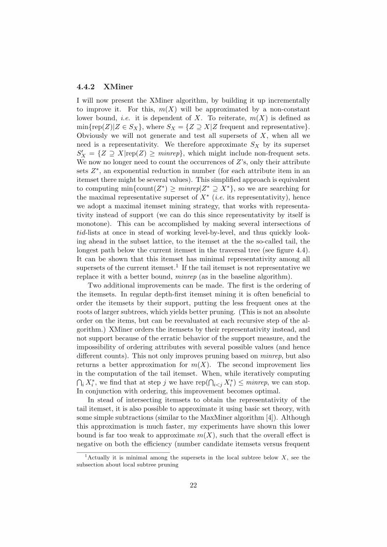
I will now present the XMiner algorithm, by building it up incrementallyto improve it. For this, m(X) will be approximated by a non-constantlower bound, i.e. it is dependent of X. To reiterate, m(X) is defined asmin{rep(Z)|Z ∈ SX}, where SX = {Z ⊇ X|Z frequent and representative}.Obviously we will not generate and test all supersets of X, when all weneed is a representativity. We therefore approximate SX by its supersetS′

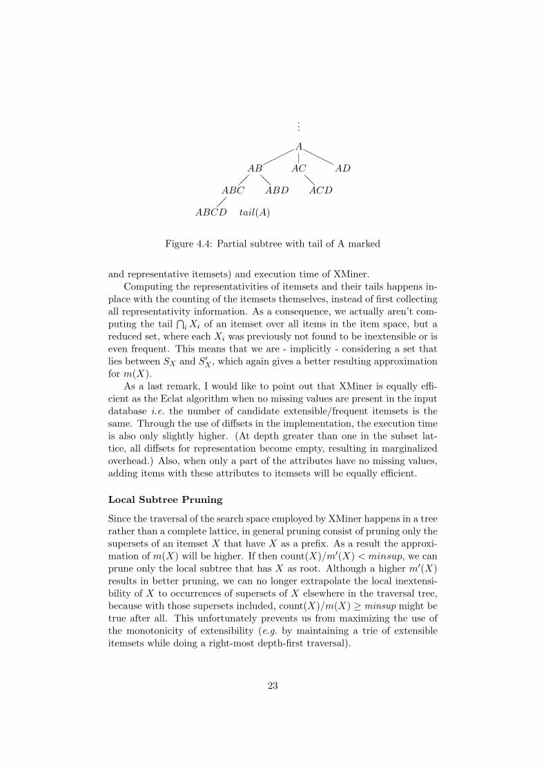
X = {Z ⊇ X|rep(Z) ≥ minrep}, which might include non-frequent sets.We now no longer need to count the occurrences of Z’s, only their attributesets Z∗, an exponential reduction in number (for each attribute item in anitemset there might be several values). This simplified approach is equivalentto computing min{count(Z∗) ≥ minrep|Z∗ ⊇ X∗}, so we are searching forthe maximal representative superset of X∗ (i.e. its representativity), hencewe adopt a maximal itemset mining strategy, that works with representa-tivity instead of support (we can do this since representativity by itself ismonotone). This can be accomplished by making several intersections oftid-lists at once in stead of working level-by-level, and thus quickly look-ing ahead in the subset lattice, to the itemset at the the so-called tail, thelongest path below the current itemset in the traversal tree (see figure 4.4).It can be shown that this itemset has minimal representativity among allsupersets of the current itemset.1 If the tail itemset is not representative wereplace it with a better bound, minrep (as in the baseline algorithm).

Two additional improvements can be made. The first is the ordering ofthe itemsets. In regular depth-first itemset mining it is often beneficial toorder the itemsets by their support, putting the less frequent ones at theroots of larger subtrees, which yields better pruning. (This is not an absoluteorder on the items, but can be reevaluated at each recursive step of the al-gorithm.) XMiner orders the itemsets by their representativity instead, andnot support because of the erratic behavior of the support measure, and theimpossibility of ordering attributes with several possible values (and hencedifferent counts). This not only improves pruning based on minrep, but alsoreturns a better approximation for m(X). The second improvement liesin the computation of the tail itemset. When, while iteratively computing⋂

i X∗

i , we find that at step j we have rep(⋂

i<j X∗

i ) ≤ minrep, we can stop.In conjunction with ordering, this improvement becomes optimal.

In stead of intersecting itemsets to obtain the representativity of thetail itemset, it is also possible to approximate it using basic set theory, withsome simple subtractions (similar to the MaxMiner algorithm [4]). Althoughthis approximation is much faster, my experiments have shown this lowerbound is far too weak to approximate m(X), such that the overall effect isnegative on both the efficiency (number candidate itemsets versus frequent

1Actually it is minimal among the supersets in the local subtree below X, see thesubsection about local subtree pruning

22

...

A

oooooooo

OOOOOOOO

AB

ÄÄÄÄ ??

??AC

????

AD

ABC

ÄÄÄÄ

ABD ACD

ABCD tail(A)

Figure 4.4: Partial subtree with tail of A marked

and representative itemsets) and execution time of XMiner.Computing the representativities of itemsets and their tails happens in-

place with the counting of the itemsets themselves, instead of first collectingall representativity information. As a consequence, we actually aren’t com-puting the tail

⋂

i Xi of an itemset over all items in the item space, but areduced set, where each Xi was previously not found to be inextensible or iseven frequent. This means that we are - implicitly - considering a set thatlies between SX and S′

X , which again gives a better resulting approximationfor m(X).

As a last remark, I would like to point out that XMiner is equally effi-cient as the Eclat algorithm when no missing values are present in the inputdatabase i.e. the number of candidate extensible/frequent itemsets is thesame. Through the use of diffsets in the implementation, the execution timeis also only slightly higher. (At depth greater than one in the subset lat-tice, all diffsets for representation become empty, resulting in marginalizedoverhead.) Also, when only a part of the attributes have no missing values,adding items with these attributes to itemsets will be equally efficient.

Local Subtree Pruning

Since the traversal of the search space employed by XMiner happens in a treerather than a complete lattice, in general pruning consist of pruning only thesupersets of an itemset X that have X as a prefix. As a result the approxi-mation of m(X) will be higher. If then count(X)/m′(X) < minsup, we canprune only the local subtree that has X as root. Although a higher m′(X)results in better pruning, we can no longer extrapolate the local inextensi-bility of X to occurrences of supersets of X elsewhere in the traversal tree,because with those supersets included, count(X)/m(X) ≥ minsup might betrue after all. This unfortunately prevents us from maximizing the use ofthe monotonicity of extensibility (e.g. by maintaining a trie of extensibleitemsets while doing a right-most depth-first traversal).

23

Algorithm 5 XMiner(set of itemsets P )



2. Representation(Xi, P )3. for all values xi of Xi with count(Xi = xi)/m′(Xi) ≥ minsup do

4. for all Xj ∈ P with Xj > Xi do



7. (Xij = xij).tids = (Xi = xi).tids ∩ (Xj = xj).tids8. if count(Xij = xij)/m′(Xi) ≥ minsup then


11. report (Xij = xij) as frequent12. XMiner(P i)


1. (X = ∗).tids = (Xi = ∗).tids2. m′(Xi) = count(X = ∗)3. for all Xj ∈ P with Xj > Xi do

4. compute (Xij = ∗).tids = (Xi = ∗).tids ∩ (Xj = ∗).tids5. if m′(Xi) > minrep then

6. (X = ∗).tids ∩ = (Xij = ∗).tids7. m′(Xi) = max(count(X = ∗),minrep)

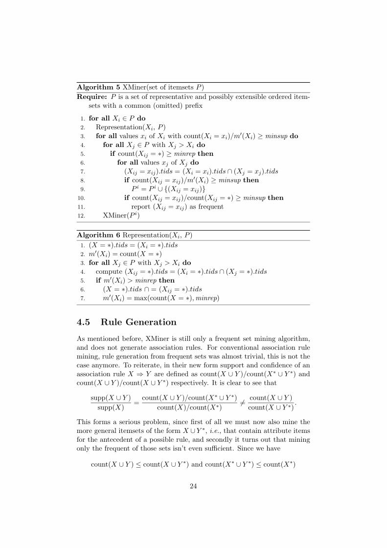
4.5 Rule Generation

As mentioned before, XMiner is still only a frequent set mining algorithm,and does not generate association rules. For conventional association rulemining, rule generation from frequent sets was almost trivial, this is not thecase anymore. To reiterate, in their new form support and confidence of anassociation rule X ⇒ Y are defined as count(X ∪ Y )/count(X∗ ∪ Y ∗) andcount(X ∪ Y )/count(X ∪ Y ∗) respectively. It is clear to see that

supp(X ∪ Y )

supp(X)=

count(X ∪ Y )/count(X∗ ∪ Y ∗)

count(X)/count(X∗)6=

count(X ∪ Y )

count(X ∪ Y ∗).

This forms a serious problem, since first of all we must now also mine themore general itemsets of the form X ∪ Y ∗, i.e., that contain attribute itemsfor the antecedent of a possible rule, and secondly it turns out that miningonly the frequent of those sets isn’t even sufficient. Since we have

count(X ∪ Y ) ≤ count(X ∪ Y ∗) and count(X∗ ∪ Y ∗) ≤ count(X∗)

24

we cannot derive any relationship between supp(X ∪ Y ) and supp(X ∪ Y ∗),due to the lack of monotonicity. So we must choose an order in which weevaluate these sets. If we first verify that X ∪Y is infrequent, we won’t haveto look at X ∪ Y ∗ since no rules can be formed. Conversely we could firstcount X∗ ∪ Y ∗ and then X ∪ Y ∗. . . , systematically replacing the attributeitems with values. The former approach clearly makes more sense, after allfor the latter approach it is possible that after replacing all attribute itemsin an itemset X∗ ∪ Y ∗ there is no frequent set X ∪ Y making all previouswork useless. Subsequently, experimentation has shown this intuition to becorrect.

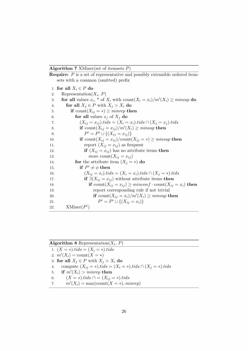
Now, if X ∪ Y is frequent we do not actually have to replace all pos-sible items with attribute items. We don’t even really need the supportof the sets X ∪ Y ∗, just their count, and count is monotone with respectto generalization of itemsets. This way we can avoid evaluating general-ized itemsets (that are partitions of ‘normal’ itemsets), that won’t formconfident rules. This is the basic idea behind the rule generating versionof XMiner. For example, if an itemset {(A=a),(B=b),(C=c)} turns outto be frequent and representative, we remember its count. Then we sys-tematically proceed with {(A=a),(B=b),(C=*)} etc. If we then find thatcount({(A=a),(B=b),(C=*)})·minconf > count({(A=a),(B=b),(C=c)}) (iethe rule (A = a), (B = b) ⇒ (C = c) is not confident) we don’t have to do{(A = a), (B = ∗), (C = ∗)} anymore since its count will be even larger, and(A = a) ⇒ (B = b), (C = c) won’t be confident either.

The pseudo-code for XMiner, extended with rule generation is depictedbelow.

25

Algorithm 7 XMiner(set of itemsets P )



2. Representation(Xi, P )3. for all values xi, * of Xi with count(Xi = xi)/m′(Xi) ≥ minsup do

4. for all Xj ∈ P with Xj > Xi do



7. (Xij = xij).tids = (Xi = xi).tids ∩ (Xj = xj).tids8. if count(Xij = xij)/m′(Xi) ≥ minsup then


11. report (Xij = xij) as frequent12. if (Xij = xij) has no attribute items then

13. store count(Xij = xij)14. for the attribute item (Xj = ∗) do

15. if P i 6= φ then

16. (Xij = xi).tids = (Xi = xi).tids ∩ (Xj = ∗).tids17. if ∃(Xij = xij) without attribute items then

18. if count(Xij = xij) ≥ minconf · count(Xij = xi) then

19. report corresponding rule if not trivial20. if count(Xij = xi)/m′(Xi) ≥ minsup then

21. P i = P i ∪ {(Xij = xi)}22. XMiner(P i)


1. (X = ∗).tids = (Xi = ∗).tids2. m′(Xi) = count(X = ∗)3. for all Xj ∈ P with Xj > Xi do

4. compute (Xij = ∗).tids = (Xi = ∗).tids ∩ (Xj = ∗).tids5. if m′(Xi) > minrep then

6. (X = ∗).tids ∩ = (Xij = ∗).tids7. m′(Xi) = max(count(X = ∗),minrep)

26

Chapter 5

Experimental Results

The XMiner algorithm and the baseline algorithm were tested and comparedagainst each other, on three different databases. The first one is the Sickdata set about Thyroid Disease1. This database contains 2800 tuples, has24 attributes and contains some missing values. The second dataset are theresults of the Eurovision song contest from 1957 to 20052. In this Europeancontest a limited number of countries can enter and give points to the others,the countries that perform worst cannot enter in the next edition. Over theyears more countries could join, recently a semi-final was introduced andcountries that do not enter can now cast votes, which was previously notpossible. This makes that the database has a lot of missing values. The formis as follows: each tuple represents a year-country combination, and has 2*43attributes for points given to and received from other countries. The thirddatabase is the Census Income dataset3. This is a large database, about100MB in size. It has 33 nominal attributes (after 7 continuous attributeswere removed) and nearly 200k tuples. Some attributes have no missingvalues, other attribute values are missing in up to 50% of the tuples. Toinvestigate the influence of missingness on XMiner, I incrementally createdseveral versions of the database, each with more values of attributes turnedinto nulls.

I implemented both XMiner and the baseline algorithm in C++ (usingdiffsets to optimize for speed [15]), compiled them with gcc 3.4.6 (all withoptimization -O3), on a machine with an AMD Opteron 64 bit CPU at 2.2GHz, with 2GB of memory, running Gentoo Linux.

1Available from the UCI Machine Learning Repository [5]2Collected and preprocessed by Joost Kok3Available from the UCI KDD Archive [7]

27

5.1 Sick Dataset

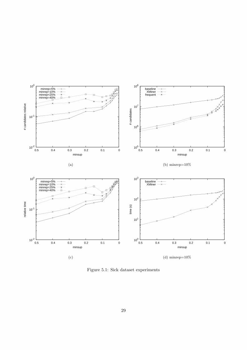
On the Sick dataset the minimum representativity was fixed at 5%, 10%,25% and 40%, and the minsup was varied each time, to look at the number ofcandidate itemsets and the execution time of XMiner, relative to the baselinealgorithm. From figure 5.1(a) it is clear that XMiner always outperformsthe baseline, while 5.1(b) shows the actual number of candidate itemsetsof the baseline and XMiner, versus the number of resulting frequent (andrepresentative) itemsets that both algorithms have as output. It shows thatXMiner follows quite closely the number of frequent itemsets, while thebaseline generates a lot more candidates than necessary, and its course israther independent of the number of frequent itemsets. Figures 5.1(c) and5.1(d) show the execution time of the same experiments. They indicate thatthe execution time corresponds to the number of generated itemsets. Thefact that the Sick dataset has some attributes without any missing values,results in a good performance of XMiner, while the baseline algorithm cannoteven take advantage of this.

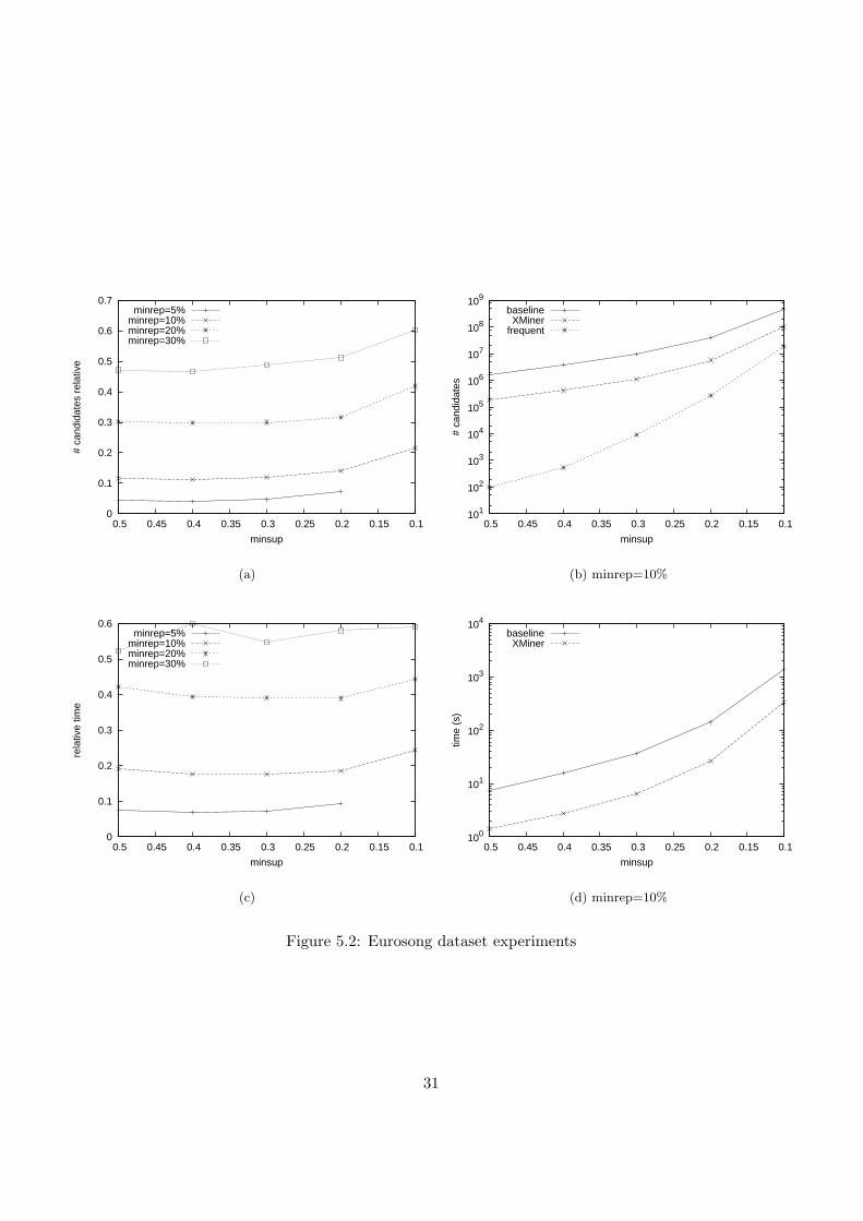
5.2 Eurosong Dataset

Similar experiments as with the sick database were performed on the Eu-rosong dataset, with several fixed minreps 5%, 10%, 20% and 30%. Forthe baseline algorithm with parameters minrep=5% and minsup=10%, theprocess was killed after 4000 seconds, so no comparison with XMiner couldbe made, and this point is not plotted (figures 5.2(a) and 5.2(c)). This timeXMiner’s course does not follow the number of representative and frequentitemsets that closely, but still outperforms the baseline algorithm by almostan order of magnitude in generated itemsets (figure 5.2(b)), and a factor ofeight in execution time (figure 5.2(d)). The eurosong dataset has more miss-ing values than the sick database (in fact for each attribute there is at leastone tuple with a missing value for that attribute). This is why the graphsof the eurosong dataset do not look as spectacular as the sick dataset, butXMiner obviously still outperforms the baseline algorithm.

Some interesting frequent sets emerged from mining the Eurosong data.I used both this version of the set, and another one with (only) 50 tuplesand 1849 (!) attributes for each country-country combination (representingpoints given). Among others I found that the United Kingdom is ratherpopular. The itemset corresponding to the UK getting points from an-other country participating in the same year, or any country after the ruleschanged in 2004 (notice the need for accounting for nulls) is 67.8%. Onthe other part of this spectrum we find Finland, for which the itemset cor-responding to not getting any points from other participating countries is70.7%. (Note that this dataset did not yet include the results from the 2006

28

10-2

10-1

100

0 0.1 0.2 0.3 0.4 0.5

# ca

ndid

ates

rel

ativ

e

minsup

minrep=5%minrep=10%minrep=25%minrep=40%

(a)

105

106

107

108

0 0.1 0.2 0.3 0.4 0.5

# ca

ndid

ates

minsup

baselineXMiner

frequent

(b) minrep=10%

10-2

10-1

100

0 0.1 0.2 0.3 0.4 0.5

rela

tive

time

minsup


(c)

100

101

102

103

0 0.1 0.2 0.3 0.4 0.5

time

(s)

minsup

baselineXMiner

(d) minrep=10%

Figure 5.1: Sick dataset experiments

29

edition of the contest, when Finland actually won with a ‘monster score’.)Examples from the other dataset are the following. If all three Scandina-vian countries Denmark, Norway and Sweden all enter the the competitionin the same year, the support of Denmark giving points to Norway, Nor-way giving points to Sweden, and Sweden giving points to Denmark is 30%.The support of Spain and Andorra giving each other points is even 100%(after inspection of the database, these scores turned out to be maximal),however Andorra has only started entering the competition in 2004, makingthis itemset not very representative.

5.3 Census Income Dataset

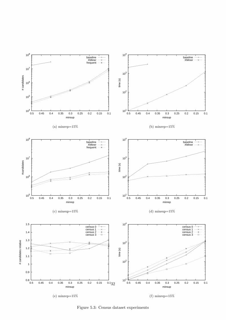
The Census database, being the largest one with nearly 200k tuples, wasmined more extensively. It was mined for varying minsup, minrep, and de-gree of missingness in the database. First, minrep was fixed at 15% andminsup varied between %50 and 10%, and the original database was used(figures 5.3(a) and 5.3(b)). Only for a minsup of 50% and 40% did thebaseline algorithm finish within 4000 seconds. Still, from this data alonewe can already see the phenomenal difference with XMiner, and also theefficiency of XMiner by itself, the number of generated candidate itemsetsfollows the frequent ones very closely. Second, minsup was fixed at 15% andexperiments were run for different minreps (figures 5.3(c) and 5.3(d)). Tostay within reasonable time, Census 3 database was used (the one with themost values removed). For a decreasing minrep the number of frequent andrepresentative itemsets does not increase dramatically. The number of gen-erated candidate itemsets by XMiner increases with a similar slope, whilethe baseline algorithm seems to generate increasingly more candidates. Thisis visible in both execution time and number of generated itemsets. Finallythe degree of missingness in the Census database was varied, by incremen-tally removing certain values of attributes (figures 5.3(e) and 5.3(f)). Dueto the lack of data from the baseline algorithm for most of these datasets, Icompared the number of candidate itemsets of XMiner versus the requirednumber of frequent and representative itemsets in the output. All graphsare rather entangled, but the number of excessively generated sets alwaysseems to remain in the 10% to 30% region.

30

0

0.1

0.2

0.3

0.4

0.5

0.6

0.7

0.1 0.15 0.2 0.25 0.3 0.35 0.4 0.45 0.5

# ca

ndid

ates

rel

ativ

e

minsup


(a)

101

102

103

104

105

106

107

108

109

0.1 0.15 0.2 0.25 0.3 0.35 0.4 0.45 0.5

# ca

ndid

ates

minsup

baselineXMiner

frequent

(b) minrep=10%

0

0.1

0.2

0.3

0.4

0.5

0.6

0.1 0.15 0.2 0.25 0.3 0.35 0.4 0.45 0.5

rela

tive

time

minsup


(c)

100

101

102

103

104

0.1 0.15 0.2 0.25 0.3 0.35 0.4 0.45 0.5

time

(s)

minsup

baselineXMiner

(d) minrep=10%

Figure 5.2: Eurosong dataset experiments

31

104

105

106

107

108

0.1 0.15 0.2 0.25 0.3 0.35 0.4 0.45 0.5

# ca

ndid

ates

minsup

baselineXMiner

frequent

(a) minrep=15%

101

102

103

104

0.1 0.15 0.2 0.25 0.3 0.35 0.4 0.45 0.5

time

(s)

minsup

baselineXMiner

(b) minrep=15%

105

106

107

108

0.1 0.15 0.2 0.25 0.3 0.35 0.4 0.45 0.5

#can

dida

tes

minrep

baselineXMiner

frequent

(c) minsup=15%

101

102

103

104

0.1 0.15 0.2 0.25 0.3 0.35 0.4 0.45 0.5

time

(s)

minrep

baselineXMiner

(d) minsup=15%

0.8

0.9

1

1.1

1.2

1.3

1.4

1.5

0.1 0.15 0.2 0.25 0.3 0.35 0.4 0.45 0.5

# ca

ndid

ates

rel

ativ

e

minsup

census 0census 1census 2census 3

(e) minrep=15%

101

102

103

104

0.1 0.15 0.2 0.25 0.3 0.35 0.4 0.45 0.5

time

(s)

minsup

census 0census 1census 2census 3

(f) minrep=15%

Figure 5.3: Census dataset experiments

32

Chapter 6

Conclusions

In this work I researched association rule mining on databases with missingvalues. Since the conventional measures and algorithms were defined fordatasets without nulls, the usual approach is to preprocess the dataset inorder to obtain a complete one. This has however a negative effect on theresults.

Therefore new itemset and association rule measures were introduced [8],that are almost obvious but seem to work very well. In particular supportand confidence were extended and a new measure, representativity, was in-troduced. Unfortunately the new support is not monotone, and confidencecannot be expressed in terms of support anymore. To overcome the firstproblem I introduced the extensibility property for itemsets, that can re-place the role of support in an algorithm, because it is monotone and linkedto support itself. I implemented this in the XMiner algorithm, which wasshown to be efficient when compared to a baseline algorithm through exper-imentation. It is a generally applicable algorithm in that it reverts back tothe Eclat algorithm if the input database contains no nulls. A basic solu-tion for the rule generation problem was also provided. For this, generalizeditemsets containing attribute items, have to be mined as well as normalitemsets, some of them might even be infrequent. By making use of themonotonicity of the absolute support count of an itemset, the number of ex-tra itemsets that need to be considered can be reduced to the sets necessaryfor generating confident rules.

In my opinion this approach is to be preferred over preprocessing an in-complete database, because of the straightforwardness, not too complicatedimplementation, and it removes the overhead of first having to do the pre-processing itself. There is however room for improvement and optimization,especially for the rule generation algorithm. This can provide for interestingfuture work.

33

Bibliography

[1] R. Agrawal, T. Imielinski, and A. Swami. Mining association rulesbetween sets of items in large databases. In Proc. ACM SIGMOD,pages 207–216, 1993.

[2] R. Agrawal, T. Imielinski, and A.N. Swami. Mining association rulesbetween sets of items in large databases. In Proc. ACM SIGMOD,pages 207–216, 1993.

[3] R. Agrawal and R. Srikant. Fast algorithms for mining association rules.In Proceedings of the 20th International Conference on Very Large Data

Bases, pages 478–499, 1994.

[4] R. J. Bayardo. Efficiently mining long patterns from databases. InProc. ACM SIGMOD, pages 85–93, Seattle, Washington, 1998.

[5] C.L. Blake D.J. Newman, S. Hettich and C.J. Merz. UCI repository ofmachine learning databases, 1998.

[6] J. Han, J. Pei, Y. Yin, and R. Mao. Mining frequent patterns withoutcandidate generation: A frequent-pattern tree approach. Data Mining

and Knowledge Discovery, 2003. To appear.

[7] S. Hettich and S. D. Bay. The UCI KDD Archive[http://kdd.ics.uci.edu] Irvine, CA: University of California, Dept. ofinf. and comp. science, 1999.

[8] A. Ragel and B. Cremillieux. Treatment of missing values for associatiorules. In Research and Development in Knowledge Discovery and Data

Mining, LNAI, 1998.

[9] D. Rubin. Inference and missing data. Biometrika, 63:581–592, 1976.

[10] A. Savasere, E. Omiecinski, and S. Navathe. An efficient algorithmfor mining association rules in large databases. In Proceedings of the

21st International Conference on Very Large Databases, pages 432–444,1995.

34

[11] R. Srikant and R. Agrawal. Mining generalized association rules. pages407–419, 1995.

[12] M. J. Zaki and K. Gouda. Fast vertical mining using diffsets. 2001.

[13] M. J. Zaki, S. Parthasarathy, M. Ogihara, and W. Li. New algorithmsfor fast discovery of association rules. In Proceedings of the Third In-

ternational Conference on Knowledge Discovery in Databases and Data

Mining, pages 283–286, 1997.

[14] M.J. Zaki. Scalable algorithms for association mining. IEEE Transac-

tions on Knowledge and Data Engineering, 12(3):372–390, May/June2000.

[15] M.J. Zaki and K. Gouda. Fast vertical mining using diffsets. In Proceed-

ings of the Ninth ACM SIGKDD International Conference on Knowl-

edge Discovery and Data Mining. ACM, 2003.

35

Documents

universiteit antwerpen