Section 2 – MicaSense 5-band MultiSpectral Imagery

USGS National UAS Project Office – March 2017

Unmanned Aircraft Systems

Data Post-Processing

Structure-from-Motion

Photogrammetry

Synopsis In this introductory training class, we will explore how to utilize image data captured from an unmanned aerial vehicle equipped with an on-board camera or sensor. Utilizing Computer Vision –Structure-from-Motion (Photogrammetry) techniques that estimates three-dimensional information from two-dimensional images. Using real world data captured from a UAS, we will illustrate how it is possible to generate georeferenced point clouds, digital surface elevation models and mosaiced image bases for mapping and geographic information system data layer creation.

Requirements Computer (desktop or laptop) with at least 8GB RAM A registered version of Agisoft PhotoScan Version 1.2.6 (Build 2834) Access the data files noted below No previous experience with PhotoScan is necessary

Workflow The following step-by-step instructions are intended to familiarize participants with the relevant components of PhotoScan. A short description is given, followed by a specific “cookbook” of instructions for how to process a dataset from beginning to end.

Data A real world dataset is provided for the exercise to see how actual collected data is processed into workable GIS data layers.

Class Outline - Import images collected from a UAS- Align the images- Create a sparse point cloud from the images- Reduce and adjust errors in the data- Create a dense point cloud- Create a mesh or digital surface model- Create image texture- Create products- Output the products for use in GIS

2

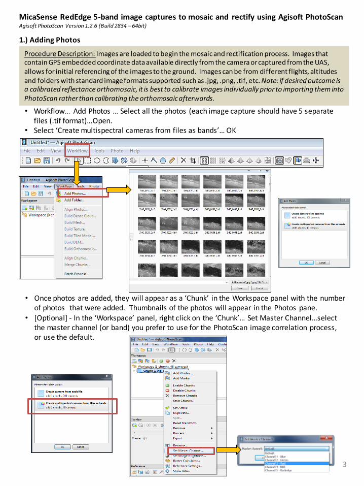
MicaSense RedEdge 5-band image captures to mosaic and rectify using Agisoft PhotoScanAgisoft PhotoScan Version 1.2.6 (Build 2834 – 64bit)

1.) Adding Photos

• Once photos are added, they will appear as a ‘Chunk’ in the Workspace panel with the number of photos that were added. Thumbnails of the photos will appear in the Photos pane.

• [Optional] - In the ‘Workspace’ panel, right click on the ‘Chunk’… Set Master Channel…select the master channel (or band) you prefer to use for the PhotoScan image correlation process, or use the default.

• Workflow… Add Photos … Select all the photos (each image capture should have 5 separate files (.tif format)…Open.

• Select ‘Create multispectral cameras from files as bands’… OK

Procedure Description: Images are loaded to begin the mosaic and rectification process. Images that contain GPS embedded coordinate data available directly from the camera or captured from the UAS, allows for initial referencing of the images to the ground. Images can be from different flights, altitudes and folders with standard image formats supported such as .jpg, .png, .tif, etc. Note: if desired outcome is a calibrated reflectance orthomosaic, it is best to calibrate images individually prior to importing them into PhotoScan rather than calibrating the orthomosaic afterwards.

3

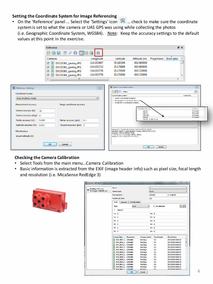
Checking the Camera Calibration• Select Tools from the main menu…Camera Calibration• Basic information is extracted from the EXIF (image header info) such as pixel size, focal length

and resolution (i.e. MicaSense RedEdge 3)

4

Setting the Coordinate System for Image Referencing• On the ‘Reference’ panel … Select the ‘Settings’ icon … check to make sure the coordinate

system is set to what the camera or UAS GPS was using while collecting the photos (i.e. Geographic Coordinate System, WGS84). Note: Keep the accuracy settings to the default values at this point in the exercise.

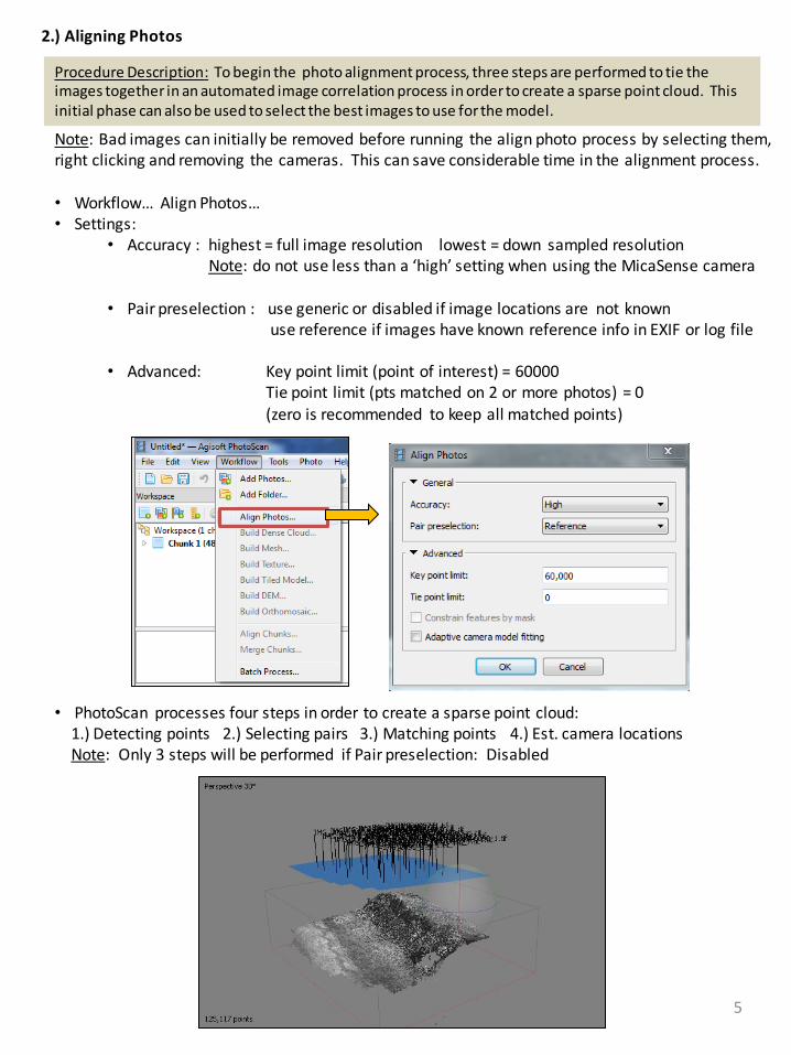
2.) Aligning Photos

• PhotoScan processes four steps in order to create a sparse point cloud: 1.) Detecting points 2.) Selecting pairs 3.) Matching points 4.) Est. camera locationsNote: Only 3 steps will be performed if Pair preselection: Disabled

Procedure Description: To begin the photo alignment process, three steps are performed to tie the images together in an automated image correlation process in order to create a sparse point cloud. This initial phase can also be used to select the best images to use for the model.

Note: Bad images can initially be removed before running the align photo process by selecting them, right clicking and removing the cameras. This can save considerable time in the alignment process.

• Workflow… Align Photos…• Settings:

• Accuracy : highest = full image resolution lowest = down sampled resolution Note: do not use less than a ‘high’ setting when using the MicaSense camera

• Pair preselection : use generic or disabled if image locations are not knownuse reference if images have known reference info in EXIF or log file

• Advanced: Key point limit (point of interest) = 60000Tie point limit (pts matched on 2 or more photos) = 0(zero is recommended to keep all matched points)

5

6

3.) Optimizing the Photo Alignment

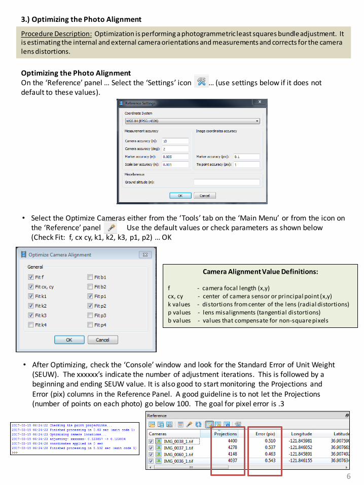
Optimizing the Photo Alignment On the ‘Reference’ panel … Select the ‘Settings’ icon … (use settings below if it does not default to these values).

Procedure Description: Optimization is performing a photogrammetric least squares bundle adjustment. It is estimating the internal and external camera orientations and measurements and corrects for the camera lens distortions.

• Select the Optimize Cameras either from the ‘Tools’ tab on the ‘Main Menu’ or from the icon on the ‘Reference’ panel Use the default values or check parameters as shown below (Check Fit: f, cx cy, k1, k2, k3, p1, p2) … OK

Camera Alignment Value Definitions:

f - camera focal length (x,y)cx, cy - center of camera sensor or principal point (x,y)k values - distortions from center of the lens (radial distortions)p values - lens misalignments (tangential distortions)b values - values that compensate for non-square pixels

• After Optimizing, check the ‘Console’ window and look for the Standard Error of Unit Weight (SEUW). The xxxxxx’s indicate the number of adjustment iterations. This is followed by a beginning and ending SEUW value. It is also good to start monitoring the Projections and Error (pix) columns in the Reference Panel. A good guideline is to not let the Projections (number of points on each photo) go below 100. The goal for pixel error is .3

4.) Error Reduction - Gradual Selection

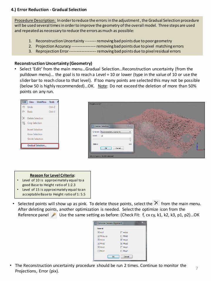
Procedure Description: In order to reduce the errors in the adjustment , the Gradual Selection procedure will be used several times in order to improve the geometry of the overall model. Three steps are used and repeated as necessary to reduce the errors as much as possible:

1. Reconstruction Uncertainty -------- removing bad points due to poor geometry2. Projection Accuracy ------------------ removing bad points due to pixel matching errors3. Reprojection Error -------------------- removing bad points due to pixel residual errors

• Selected points will show up as pink. To delete those points, select the from the main menu.After deleting points, another optimization is needed. Select the optimize icon from the Reference panel Use the same setting as before: (Check Fit: f, cx cy, k1, k2, k3, p1, p2)…OK

Reason for Level Criteria:• Level of 10 is approximately equal to a

good Base to Height ratio of 1:2.3• Level of 15 is approximately equal to an

acceptable Base to Height ratio of 1: 5.5

• The Reconstruction uncertainty procedure should be run 2 times. Continue to monitor the Projections, Error (pix).

Reconstruction Uncertainty (Geometry)• Select ‘Edit’ from the main menu…Gradual Selection…Reconstruction uncertainty (from the

pulldown menu)… the goal is to reach a Level = 10 or lower (type in the value of 10 or use the slider bar to reach close to that level). If too many points are selected this may not be possible (below 50 is highly recommended)…OK. Note: Do not exceed the deletion of more than 50% points on any run.

7

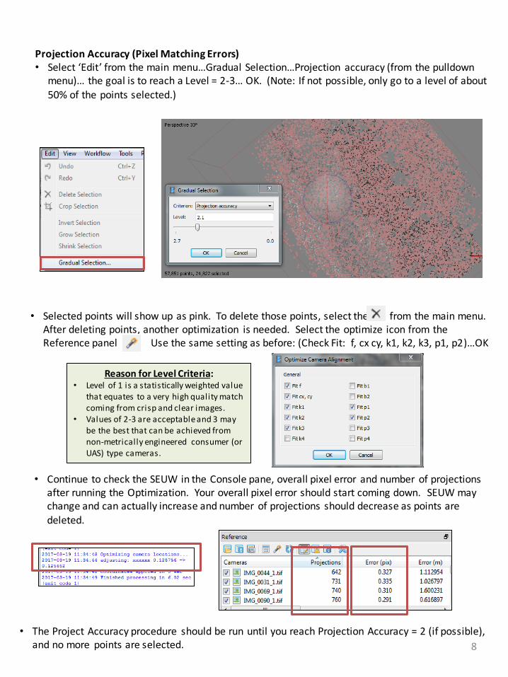
Projection Accuracy (Pixel Matching Errors)• Select ‘Edit’ from the main menu…Gradual Selection…Projection accuracy (from the pulldown

menu)… the goal is to reach a Level = 2-3… OK. (Note: If not possible, only go to a level of about 50% of the points selected.)

• Selected points will show up as pink. To delete those points, select the from the main menu.After deleting points, another optimization is needed. Select the optimize icon from the Reference panel Use the same setting as before: (Check Fit: f, cx cy, k1, k2, k3, p1, p2)…OK

8

• Continue to check the SEUW in the Console pane, overall pixel error and number of projections after running the Optimization. Your overall pixel error should start coming down. SEUW may change and can actually increase and number of projections should decrease as points are deleted.

Reason for Level Criteria:• Level of 1 is a statistically weighted value

that equates to a very high quality match coming from crisp and clear images.

• Values of 2-3 are acceptable and 3 may be the best that can be achieved from non-metrically engineered consumer (or UAS) type cameras.

• The Project Accuracy procedure should be run until you reach Projection Accuracy = 2 (if possible), and no more points are selected.

9

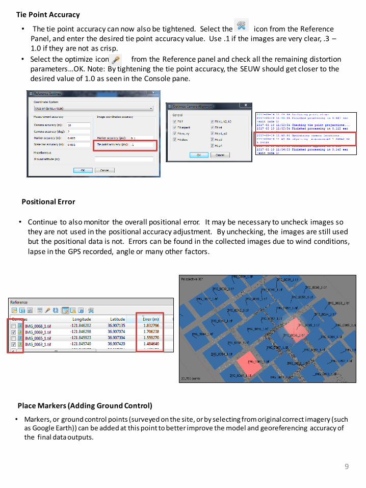
• Select the optimize icon from the Reference panel and check all the remaining distortion parameters…OK. Note: By tightening the tie point accuracy, the SEUW should get closer to the desired value of 1.0 as seen in the Console pane.

Tie Point Accuracy

• The tie point accuracy can now also be tightened. Select the icon from the Reference Panel, and enter the desired tie point accuracy value. Use .1 if the images are very clear, .3 –1.0 if they are not as crisp.

• Continue to also monitor the overall positional error. It may be necessary to uncheck images so they are not used in the positional accuracy adjustment. By unchecking, the images are still used but the positional data is not. Errors can be found in the collected images due to wind conditions, lapse in the GPS recorded, angle or many other factors.

Positional Error

Place Markers (Adding Ground Control)

• Markers, or ground control points (surveyed on the site, or by selecting from original correct imagery (such as Google Earth)) can be added at this point to better improve the model and georeferencing accuracy of the final data outputs.

10

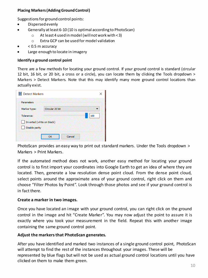
Placing Markers (Adding Ground Control)

Suggestions for ground control points: Dispersed evenly

Generally at least 6-10 (10 is optimal according to PhotoScan)

o At least 4 used in model (will not work with < 3)

o Extra GCP can be used for model validation

< 0.5 m accuracy

Large enough to locate in imagery

Identify a ground control point

There are a few methods for locating your ground control. If your ground control is standard (circular12 bit, 16 bit, or 20 bit, a cross or a circle), you can locate them by clicking the Tools dropdown >

Markers > Detect Markers. Note that this may identify many more ground control locations than

actually exist.

PhotoScan provides an easy way to print out standard markers. Under the Tools dropdown >

Markers > Print Markers.

If the automated method does not work, another easy method for locating your ground

control is to first import your coordinates into Google Earth to get an idea of where they arelocated. Then, generate a low resolution dense point cloud. From the dense point cloud,

select points around the approximate area of your ground control, right click on them and

choose “Filter Photos by Point”. Look through those photos and see if your ground control is

in fact there.

Create a marker in two images.

Once you have located an image with your ground control, you can right click on the ground

control in the image and hit “Create Marker”. You may now adjust the point to assure it isexactly where you took your measurement in the field. Repeat this with another image

containing the same ground control point.

Adjust the markers that PhotoScan generates.

After you have identified and marked two instances of a single ground control point, PhotoScanwill attempt to find the rest of the instances throughout your images. These will be represented by blue flags but will not be used as actual ground control locations until you have clicked on them to make them green.

11

Note: If your ground control is out of focus in the image and you are unsure of where to put

your marker, it might be better not to place a marker than to place one incorrectly!

Repeat for all ground control locations.

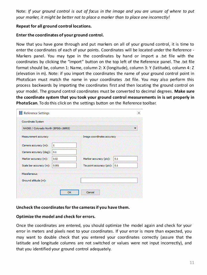
Enter the coordinates of your ground control.

Now that you have gone through and put markers on all of your ground control, it is time toenter the coordinates of each of your points. Coordinates will be located under the Reference -

Markers panel. You may type in the coordinates by hand or import a .txt file with thecoordinates by clicking the “import” button on the top left of the Reference panel. The .txt file

format should be, column 1: Name, column 2: X (longitude), column 3: Y (latitude), column 4: Z(elevation in m). Note: if you import the coordinates the name of your ground control point in

PhotoScan must match the name in your coordinates .txt file. You may also perform thisprocess backwards by importing the coordinates first and then locating the ground control on

your model. The ground control coordinates must be converted to decimal degrees. Make sure

the coordinate system that you took your ground control measurements in is set properly inPhotoScan. To do this click on the settings button on the Reference toolbar.

Uncheck the coordinates for the cameras if you have them.

Optimize the model and check for errors.

Once the coordinates are entered, you should optimize the model again and check for yourerror in meters and pixels next to your coordinates. If your error is more than expected, you

may want to double check that you entered your coordinates correctly (assure that thelatitude and longitude columns are not switched or values were not input incorrectly), and

that you identified your ground control adequately.

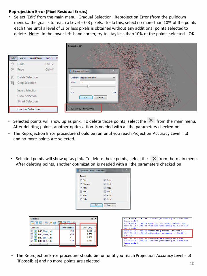
• The Reprojection Error procedure should be run until you reach Projection Accuracy Level = .3 and no more points are selected.

Reprojection Error (Pixel Residual Errors)• Select ‘Edit’ from the main menu…Gradual Selection…Reprojection Error (from the pulldown

menu)… the goal is to reach a Level = 0.3 pixels. To do this, select no more than 10% of the points each time until a level of .3 or less pixels is obtained without any additional points selected to delete. Note: in the lower left-hand corner, try to stay less than 10% of the points selected …OK.

• Selected points will show up as pink. To delete those points, select the from the main menu.After deleting points, another optimization is needed with all the parameters checked on.

• The Reprojection Error procedure should be run until you reach Projection Accuracy Level = .3 (if possible) and no more points are selected.

• Selected points will show up as pink. To delete those points, select the from the main menu.After deleting points, another optimization is needed with all the parameters checked on

10

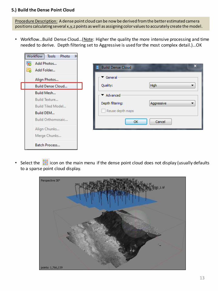
5.) Build the Dense Point Cloud

Procedure Description: A dense point cloud can be now be derived from the better estimated camera positions calculating several x,y,z points as well as assigning color values to accurately create the model.

• Workflow…Build Dense Cloud…(Note: Higher the quality the more intensive processing and time needed to derive. Depth filtering set to Aggressive is used for the most complex detail.)…OK

• Select the icon on the main menu if the dense point cloud does not display (usually defaults to a sparse point cloud display.

13

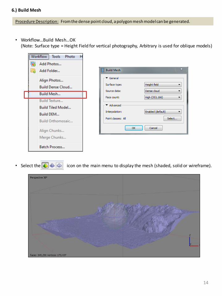
6.) Build Mesh

Procedure Description: From the dense point cloud, a polygon mesh model can be generated.

• Workflow…Build Mesh…OK(Note: Surface type = Height Field for vertical photography, Arbitrary is used for oblique models)

• Select the icon on the main menu to display the mesh (shaded, solid or wireframe).

14

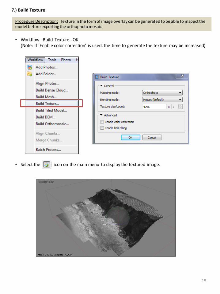
7.) Build Texture

Procedure Description: Texture in the form of image overlay can be generated to be able to inspect the model before exporting the orthophoto mosaic.

• Workflow…Build Texture…OK(Note: If ‘Enable color correction’ is used, the time to generate the texture may be increased)

• Select the icon on the main menu to display the textured image.

15

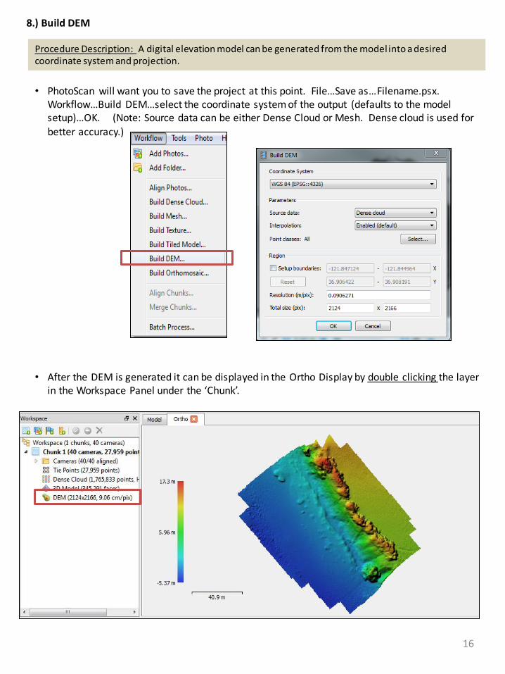
8.) Build DEM

Procedure Description: A digital elevation model can be generated from the model into a desired coordinate system and projection.

• PhotoScan will want you to save the project at this point. File…Save as…Filename.psx. Workflow…Build DEM…select the coordinate system of the output (defaults to the model setup)…OK. (Note: Source data can be either Dense Cloud or Mesh. Dense cloud is used for better accuracy.)

• After the DEM is generated it can be displayed in the Ortho Display by double clicking the layer in the Workspace Panel under the ‘Chunk’.

16

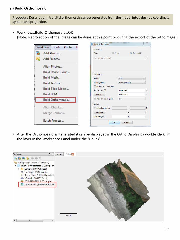
9.) Build Orthomosaic

Procedure Description: A digital orthomosaic can be generated from the model into a desired coordinate system and projection.

• Workflow…Build Orthomosaic…OK(Note: Reprojection of the image can be done at this point or during the export of the orthoimage.)

• After the Orthomosaic is generated it can be displayed in the Ortho Display by double clicking the layer in the Workspace Panel under the ‘Chunk’.

17

18

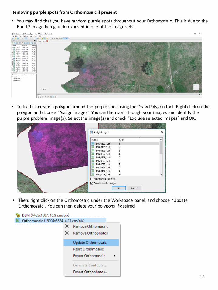
Removing purple spots from Orthomosaic if present

• You may find that you have random purple spots throughout your Orthomosaic. This is due to the Band 2 image being underexposed in one of the image sets.

• To fix this, create a polygon around the purple spot using the Draw Polygon tool. Right click on the polygon and choose “Assign Images”. You can then sort through your images and identify the purple problem image(s). Select the image(s) and check “Exclude selected images” and OK.

• Then, right click on the Orthomosaic under the Workspace panel, and choose “Update Orthomosaic”. You can then delete your polygons if desired.

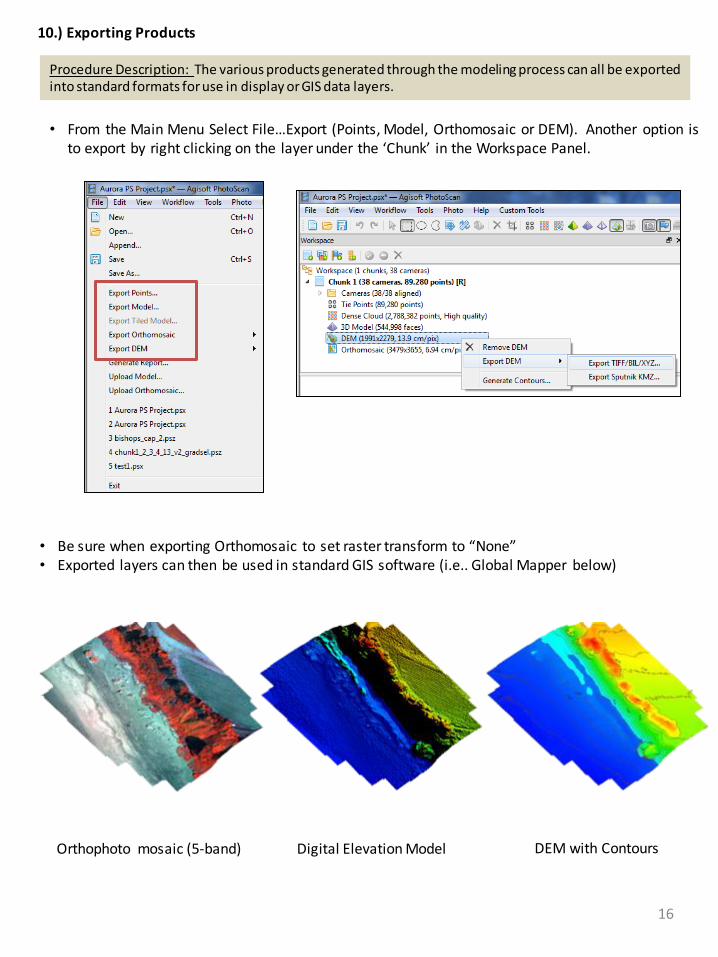
10.) Exporting Products

Procedure Description: The various products generated through the modeling process can all be exported into standard formats for use in display or GIS data layers.

• From the Main Menu Select File…Export (Points, Model, Orthomosaic or DEM). Another option is to export by right clicking on the layer under the ‘Chunk’ in the Workspace Panel.

• Be sure when exporting Orthomosaic to set raster transform to “None”• Exported layers can then be used in standard GIS software (i.e.. Global Mapper below)

Orthophoto mosaic (5-band) Digital Elevation Model DEM with Contours

16

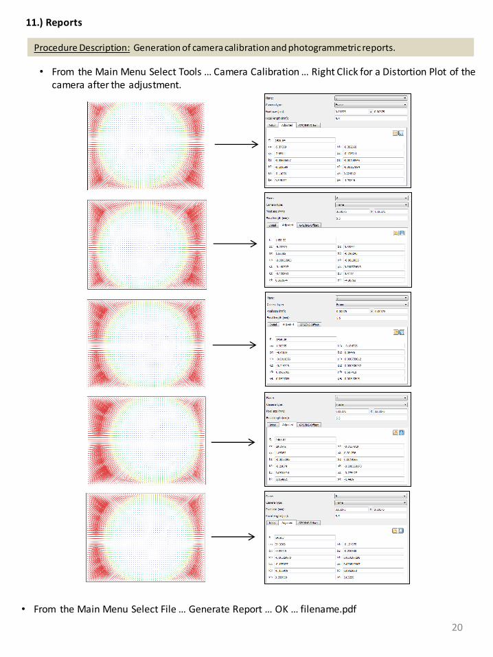
11.) Reports

Procedure Description: Generation of camera calibration and photogrammetric reports.

• From the Main Menu Select Tools … Camera Calibration … Right Click for a Distortion Plot of the camera after the adjustment.

20

• From the Main Menu Select File … Generate Report … OK … filename.pdf

21

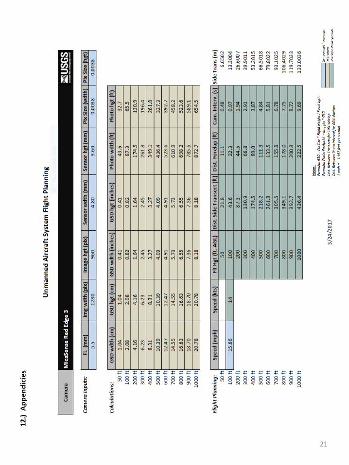
12.)

A

pp

end

icie

s