Using ArcToolbox - CIESIN · geoprocessing work using ArcToolbox. Y ou™ll still need to use ArcCatalog to manage and examine your datasets. Keep both applications open for the remainder

Using ArcToolbox™

GIS by ESRI ™

�� !��"��

#�� !��"��"$!��%"�$�� #��&��'��"��$��"�� &��"��"��(�� &��'!��)��$"��!�� !��)��!��"��"��!�"��"��"�$��"��"��)�� !��!��%"��%��!��&��)��*$��$��)��+��"�,��-.�(�&/��'�� -0-1.��

#�� !��"��"$!��$)2�"�"��&��$��"��

��

�� &��"$!��3��$��$)2�"��!�� 4�"��!��5��!��"*$��#��#�634�,�#�6��57#��!��!$!�$��$��"��"��$��)��5��!��$)2�"��"�� 8��9:��01�;��<=�(� .0>?8��9:��01� <=�(� .0>��3��8��9��3��<��!!��"��#�"��"��6��3��!�$�� &��>?��68��9�:��010��:<(@A� :><#�"��"��6��>��3��68��9��0�0��<��!�$�� &��>��"�)��"��3,��$ �"$��-.�(�&/��'�� -0-1.��

��)��!��'�� "��"�$��?��$��!!$��"�� "#��)�%��"��,4�#�B4��4@#��"5��5��)�� "�� !��'��&&&��"�!��"�!��'� ��#��C��&��!��'� ,�"��

#��!�� "�!��$"��!��'��!��'�� "��!��'�&��

Attribution.p65 08/28/2002, 11:40 AM1

IN THIS CHAPTER

7

Quick-start tutorial 2• Exercise 1: Organizing your data

in ArcCatalog

• Exercise 2: Processing the foreststands

• Exercise 3: Processing thestreams and roads

• Exercise 4: Converting data

• Exercise 5: Creating the analysiscoverage

• Exercise 6: Computing the timbervalue

Conducting a GIS processing project is easier than ever with the powerfultools in ArcToolbox. When used in conjunction with ArcCatalog�the applica-tion for browsing, storing, organizing, and distributing data�ArcToolbox letsyou meet the geoprocessing needs of your project quickly and efficiently.

In this tutorial, you�ll use ArcToolbox andArcCatalog to conduct a logging study for aportion of the Tongass National Forest in south-eastern Alaska. By performing overlays, buffers,and other geoprocessing tasks with ArcToolbox,you�ll calculate the dollar value of trees in areassuitable for logging. You�ll use ArcCatalog toorganize and manage your data, as well as toimmediately preview the results for each step.

The study area is shown here. You will conductthe study for the PetersburgB4 and PetersburgB515-minute quadrangles. You will use base cover-ages and grids for forest stands, rivers, roads, and

old growth to complete the study. This data has been provided with thesoftware. Additionally, several of the coverages you would normally derive inthe course of this project are provided to eliminate repetitive processing steps.

When conducting your analysis, you must keep certain study criteria in mind.First, harvest areas must be 100 meters from all roads and fish spawningstreams. Second, areas must not include old growth forest.

03Ch02.p65 12/18/2000, 10:30 AM7

8 USING ARCTOOLBOX

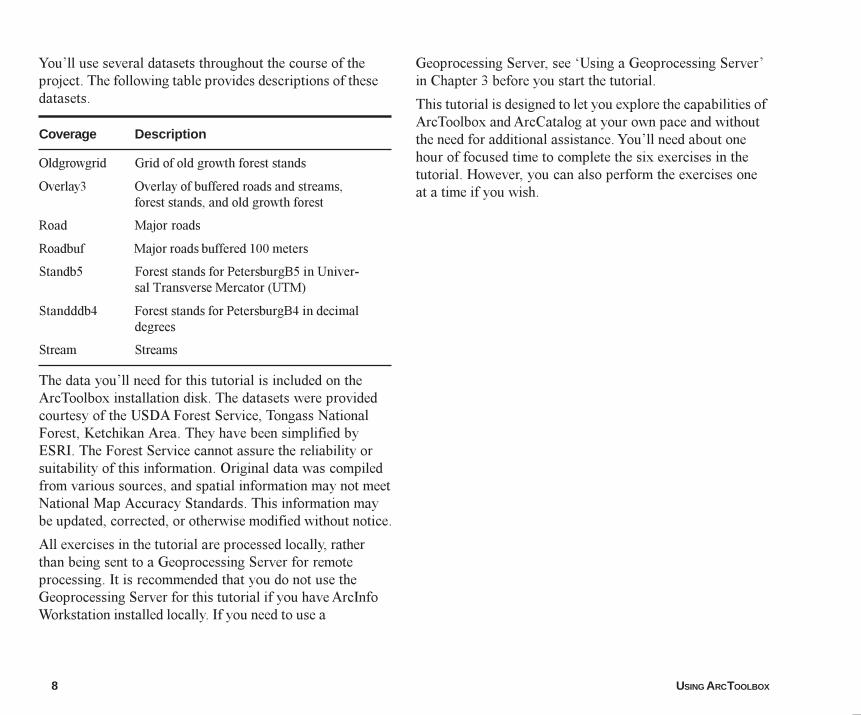
You�ll use several datasets throughout the course of theproject. The following table provides descriptions of thesedatasets.

Coverage Description

Oldgrowgrid Grid of old growth forest stands

Overlay3 Overlay of buffered roads and streams,forest stands, and old growth forest

Road Major roads

Roadbuf Major roads buffered 100 meters

Standb5 Forest stands for PetersburgB5 in Univer-sal Transverse Mercator (UTM)

Standddb4 Forest stands for PetersburgB4 in decimaldegrees

Stream Streams

The data you�ll need for this tutorial is included on theArcToolbox installation disk. The datasets were providedcourtesy of the USDA Forest Service, Tongass NationalForest, Ketchikan Area. They have been simplified byESRI. The Forest Service cannot assure the reliability orsuitability of this information. Original data was compiledfrom various sources, and spatial information may not meetNational Map Accuracy Standards. This information maybe updated, corrected, or otherwise modified without notice.

All exercises in the tutorial are processed locally, ratherthan being sent to a Geoprocessing Server for remoteprocessing. It is recommended that you do not use theGeoprocessing Server for this tutorial if you have ArcInfoWorkstation installed locally. If you need to use a

Geoprocessing Server, see �Using a Geoprocessing Server�in Chapter 3 before you start the tutorial.

This tutorial is designed to let you explore the capabilities ofArcToolbox and ArcCatalog at your own pace and withoutthe need for additional assistance. You�ll need about onehour of focused time to complete the six exercises in thetutorial. However, you can also perform the exercises oneat a time if you wish.

03Ch02.p65 11/29/2000, 3:29 PM8

QUICK-START TUTORIAL 9

Exercise 1: Organizing your data in ArcCatalog

Before you begin your geoprocessing and analysis work,you must first find and organize the data that you�ll need.You should organize your data in such a way that you�ll beable to find it quickly and efficiently. This will be doneusing ArcCatalog.

Copying and connecting to data

You�ll begin by copying the tutorial data provided with theArcToolbox software to a folder on a local disk. You willwork with a copy of the data locally if the data was in-stalled on a connected disk, in order to maintain theintegrity of the original data. Once it has been copied, youwill then create a connection to the folder containing thedata in ArcCatalog.

1. Start ArcCatalog by either double-clicking a shortcutinstalled on your desktop or using the Programs list inyour Start menu.

2. Copy the ArcToolbox tutorial data from the directorywhere it is installed to your own tutorial workspace. Inthe examples shown here, the data has been copied tolocal drive D:\ and placed in a folder called �tutorial�.

In ArcCatalog, data is accessed through folder connec-tions. When you look in a folder connection, you canquickly see the folders and data sources it contains.You�ll now begin organizing your tutorial data bycreating a folder connection to it.

3. Click the Connect To Folder button and navigate to thedata folder. Click OK to establish a folder connection.

Your new folder connection�D:\tutorial\Tongass�isnow listed in the ArcCatalog tree. You will now be ableto access all of the data needed for your project throughthat connection.

Exploring your data

Before you begin your analysis, you should explore thedatasets provided for the project. This will help you get abetter feel for ArcCatalog and the tutorial data.

1. Click the Thumbnails button on the Standard toolbar todisplay previously created thumbnail images of thedatasets in your Tongass folder.

Layers have been created for all the coverages. TheStandb5 coverage is in a UTM projection, whileStandddb4 is in unprojected decimal degrees. All othercoverages and grids have been merged and are in UTMprojection.

3

03Ch02.p65 11/29/2000, 3:29 PM9

10 USING ARCTOOLBOX

4. Right-click the VALUE-PER-METER field to open acontext menu. Sort the table into ascending and thendescending order. What is the lowest nonzero value permeter? What is the greatest?

Starting ArcToolbox

In the remaining sections of the tutorial, you�ll conduct yourgeoprocessing work using ArcToolbox. You�ll still need touse ArcCatalog to manage and examine your datasets.Keep both applications open for the remainder of thetutorial.

1. Click the Launch ArcToolbox button on the ArcCatalogtoolbar to start ArcToolbox.

2. Click the plus sign next to the D:\tutorial\Tongassconnection to see the datasets contained in the folder.Click the Preview tab and click each dataset in the tree.

3. Double-click the Standb5 coverage to open it. Click thepolygon feature class. Click the Preview dropdownarrow and click Table to see the feature attribute tablecontents. The VALUE-PER-METER field stores thevalue of the timber in each forest stand as a density�dollars per meter squared.

Polygons with a value-per-meter attribute of zero arenonforested areas such as lakes and grasslands. Be-cause the purpose of this project is to calculate the valueof trees in areas suitable for logging, you will exclude thenonforested areas from the timber harvest. You will thencompute the value of the timber in the remaining areausing this attribute.

2

3

1

4

1

03Ch02.p65 11/29/2000, 3:30 PM10


You can also start ArcToolbox as you would any otherapplication�from the Start menu or from a shortcut onyour desktop.

2. Both the ArcCatalog and ArcToolbox windows shouldnow be open. Size and arrange the two applications onyour screen so that both are visible.

You are now ready to start the first part of the tutorial:processing the forest stands. You�ll be introduced to severalArcToolbox tools and wizards and will use these for youranalysis.

03Ch02.p65 11/29/2000, 3:30 PM11

12 USING ARCTOOLBOX

Exercise 2: Processing the forest stands

In the first exercise, you prepared for the latter exercisesby organizing your data. Now you are ready to beginprocessing your data. Two forest stand coverages�Standddb4 and Standb5�currently cover the entire studyarea. Before you can begin your study, these coveragesmust be merged.

As noted in Exercise 1, the Standb5 coverage is projectedin a UTM coordinate system, while the Standddb4 coverageis in unprojected decimal degrees. In order for you toconduct a meaningful analysis of these areas, the coveragesmust share the same coordinate system. For this reason,you will project Standddb4 to match the coordinate systemof Standb5. Once this is done, the topology will have to berebuilt as it is lost when a coverage is projected.

Projecting a coverage

ArcToolbox software�s Project Wizard lets you easilyproject a coverage to another coordinate system. You canuse the Project Wizard to manually define the outputprojection (you supply all the projection parameters), or youcan have the wizard use the projection information stored inan existing coverage. For this study, you�ll use the wizard toproject the Standddb4 coverage to match the coordinatesystem of Standb5.

1. Double-click the Project Wizard (coverages, grids) in theProjections toolset of Data Management Tools.

The first panel of the Project Wizard (coverages, grids)should now be open. You will use the projection informa-tion in Standb5 to project Standddb4.

2. Click the option to Project my data to match existingdata. Click Next.

This panel is used to specify your input coverage.ArcToolbox gives you several options for setting inputand output dataset names. You can type the fullpathname to the dataset into the text box. You can alsoclick and drag a dataset, or datasets, from theArcCatalog tree or Contents tab and drop it on the textbox. Alternatively, you can click the Browse button toopen the ArcCatalog browser and navigate to yourdataset.

ArcToolbox has a feature called sticky paths. Thismeans that it remembers the path to the last dataset youspecified and will assume that the same path applieswhen you type only a dataset name into another tool orwizard. It also remembers output dataset paths.

1

03Ch02.p65 11/29/2000, 3:30 PM12


Tutorial instructions will simply ask you to type coveragenames and their paths into the appropriate text boxes.However, feel free to use any of the techniques justdescribed to make the entry.

3. Type �D:\tutorial\Tongass\Standddb4� in the Dataset textbox. Click Next.

Use the next panel of the wizard to specify the name ofthe coverage whose projection information will be usedto define the output projection. You will use Standb5 todefine it. Notice that in both this and the previous panel,the wizard displays the projection information for thecoverage you have selected.

4. Type �D:\tutorial\Tongass\Standb5� in the Dataset textbox. Click Next.

The next panel appears, where you will specify theoutput coverage name. You will call the output coverage�Standb4� and store it in your Tongass folder.

5. Type �D:\tutorial\Tongass\Standb4� for the outputdataset. Click Next. A summary page appears. Once youhave reviewed the summary, click Finish.

A message appears to tell you that the wizard is pro-cessing your request. This message appears in all toolsand wizards when a process is active. When the tool orwizard is finished, the message disappears, indicatingthat the process is complete.

Your new coverage should now appear in your Tongassfolder.

6. Click the Standb4 coverage in the Catalog tree and clickthe Preview tab. Switch to Geography on the Previewdropdown list to see your new coverage.

03Ch02.p65 11/29/2000, 3:31 PM13

14 USING ARCTOOLBOX

Building topology

If you double-click the Standb4 coverage in the ArcCatalogtree, you�ll note that the coverage doesn�t contain a poly-gon feature class. This is because changing a coverage�sprojection removes its topology. You must now rebuildpolygon topology for your new coverage using the Buildtool before going any further with your analysis.

1. Double-click the Build tool in the Topology toolset ofData Management Tools.

2. Type �D:\tutorial\Tongass\standb4� in the Input coveragetext box.

3. Change the Feature class to Poly. Click Yes on thesubsequent message box to confirm Poly as the desiredfeature class. Click OK.

The Standb4 and Standb5 coverages are now in thesame projection (UTM), and your new coverage haspolygon topology. The next step is to merge the cover-ages together so that the data can be used as onedataset that matches the extents of the other coveragesin the study.

Merging datasets

You can use the Append Wizard to merge the two cover-ages.

1. Double-click Append Wizard in the Aggregate toolset ofData Management Tools.

The Append Wizard joins multiple coverages togetherwhen you type their names in the Coverages to beappended text box. The easiest way to do this is to usethe browser and select all of the datasets at once.Simply click the coverage, then hold down the Ctrl orShift key while clicking the other coverages to selectthem all.

1

03Ch02.p65 11/29/2000, 3:31 PM14


2. Click the Browse button and navigate to theD:\tutorial\Tongass folder. Select Standb4 and Standb5and click the Open button.

Your coverages should now be listed on the wizard. Ifyou made a mistake, you can remove a coverage byselecting it and clicking the Delete button next to thelist.

3. Click Next.

The next panel of the wizard appears. You will use it tospecify the feature classes that will be merged.

4. Click Poly in the Feature classes list.

5. Click Next.

This panel is used to specify the name of an optional clipcoverage. You will not use a clip coverage in this tuto-rial.

6. Click Next.

Use the next panel to specify the output coverage nameand to offset the feature IDs. Unique feature IDswithin the output coverage are necessary in order tomaintain a relationship between the new features andthe originals.

7. Type �D:\tutorial\Tongass\stand� in the Output coveragetext box. Click the Create unique IDs dropdown arrowand click Features only. Click Next.

8. Review the summary panel and click Finish.

Your forest stand data is now ready to be used with theother Tongass datasets in the next exercise. By analyzingthe forest stand data along with the coverages you�ll createin the upcoming tasks, you will determine which areas aresuitable for harvest and how valuable those areas are.

2

03Ch02.p65 11/29/2000, 3:31 PM15

16 USING ARCTOOLBOX

In the last exercise, you processed the forest stands; nowyou will process the streams and roads data to eliminate theareas that do not meet the first of the specified criteria:harvest areas must be at least 100 meters from all fishspawning streams and roads.

To process the streams, you will first select and extractstream segments flagged as fish spawning grounds andplace them in a new coverage named Fish. You will thengenerate a 100-meter buffer around each segment.

To meet the second part of the criterium�harvest areasmust be at least 100 meters from roads�you would have tocreate a similar buffer. However, this step has already beencompleted for you to avoid repetition; the extracted roadsare represented by the Roadbuf coverage.

Extracting features

Using the Select tool, you will extract streams that areflagged as fish spawning areas to a new coverage. Butfirst, you should examine the stream coverage inArcCatalog to see how many streams are in the study area.

1. Click the Stream coverage in the ArcCatalog tree andclick the Preview tab to examine the coverage.

2. Double-click the Select tool in the Extract toolset ofAnalysis Tools.

You will now specify the coverage and feature class thatyou are processing, the logical expression that identifiesthe features (there is a button that opens a querybuilder), and the output coverage and feature class.

3. Type �D:\tutorial\Tongass\stream� in the Input coveragetext box.

4. Click the Input feature class dropdown arrow and clickLine.

Exercise 3: Processing the streams and roads

2

6

Q

3

4

5

03Ch02.p65 11/29/2000, 3:32 PM16


5. Click the first option to Build a query if it is not alreadyselected.

6. Click the Query Builder button to open the QueryBuilder dialog box.

You�ll use the Query Builder to create the logicalexpression that identifies the features you want to select.You can type the expression directly into the text box orbuild the expression by clicking the fields, operators,connectors, and values. You must choose the selectionmethod before creating the expression, as it affects theexpression�s logic. Once a suitable expression is cre-ated, you can add it to the tool�s expression list.

The default selection method is subset. If you arefamiliar with the ArcInfo TABLES� module, subset isthe same as using the RESELECT keyword when youcreate a selection expression.

7. Type the expression �AHMU-CLASS = 2� in theCurrent expression text box. Keep the default selectionmethod.

The item AHMU-CLASS is used to classify the streamtypes. All spawning streams have a value of 2. Theexpression tells the Select tool to extract only thosestreams with a value of 2�that is, the fish spawningstreams.

8. Click the down arrow button next to the Current expres-sion text box to add the expression to the list.

9. Click OK to close the Query Builder.

Call your new coverage Fish and save it in your Tongassfolder.

10. Type �D:\tutorial\Tongass\Fish� in the Output coveragetext box on the Select tool. Click OK.

A message appears when the processing is completeasking whether you want to see the output tool mes-sages. Click Yes and review the number of input andoutput lines.

You can now view your new Fish coverage inArcCatalog.

8

7

03Ch02.p65 11/29/2000, 3:32 PM17

18 USING ARCTOOLBOX

Creating a buffer

Now that you�ve created a coverage representing the fishspawning streams, you can build a 100-meter buffer aroundthem using the Buffer Wizard. You�ll end up with a newcoverage called Fishbuf.

1. Double-click Buffer Wizard in the Proximity toolset ofAnalysis Tools.

2. Click Next after reading the introductory panel. Youwant the output coverage to contain polygons, not

regions, so accept the default buffer type and clickNext.

3. Type �D:\tutorial\Tongass\Fish� as the coverage youwant to buffer. Click Next.

4. Accept the Single buffer with Specified distance optionand click Next.

5. Type �100� as the buffer distance in meters and clickNext.

6. Click Both sides with round ends for the buffer style.Click Next.

7. Type �D:\tutorial\Tongass\Fishbuf� as the output cover-age.

You must now set the inside and outside values for theoutput coverage. Inside and outside values are used todetermine which areas are inside or outside the bufferarea.

71

03Ch02.p65 11/29/2000, 3:33 PM18


8. Type �IN-FISH� as the item name. Type �1� for theinside value and �0� for the outside value. Click Nextwhen finished.

9. After reviewing your choices on the last panel, clickFinish to run the wizard.

10. View your Fishbuf coverage in ArcCatalog.

11. Examine the polygon attribute table for Fishbuf. Notethe IN-FISH field and its values. Records with an IN-FISH value of 0 indicate a polygon that is not within100 meters of a stream, while records with a value of 1are within that distance. This item and its values will beimportant in a latter step that determines what areas areavailable for forest harvesting.

As mentioned earlier, one of the timber value criteriarequires a 100-meter buffer on major roads. To makethis buffer, you would follow the same process you justfollowed to create the Fishbuf coverage.

However, to eliminate a repetitive step, the Roadbufcoverage was created for you. It is in your Tongassdirectory; use ArcCatalog to examine it. Pay particularattention to the IN-ROAD polygon attribute.

In the next exercise, you�ll create an old growth forestcoverage. This coverage, along with the Stand, Fishbuf, andRoadbuf coverages, will be used to generate the finalresults.

03Ch02.p65 11/29/2000, 3:33 PM19

20 USING ARCTOOLBOX

In the previous exercises, you processed forest stands,streams, and roads to help in your study. Now, you�llconvert the grid of old growth forest areas into a coveragethat will be used in an overlay with the forest stands. Thisgrid was created exclusively for this tutorial; it was notprovided by the Forest Service.

You�ll use the Grid to Polygon Coverage tool to completethe conversion.

1. Double-click Grid to Polygon Coverage in the Exportfrom Raster toolset in Conversion Tools.

2. Type �D:\tutorial\Tongass\oldgrowgrid� in the Input gridtext box. Type �D:\tutorial\Tongass\Oldgrow� in theOutput coverage text box. Click OK.

Exercise 4: Converting data

When the tool is finished processing the request, youshould see your new coverage, Oldgrow, in theArcCatalog tree.

3. Click the Preview tab in ArcCatalog to view theOldgrow coverage in Preview view. Zooming in revealsthe common stair-step effect found in vector data thathas been converted from raster data.

4. Examine the attributes for the coverage�s polygonfeature class. Areas of old growth have a GRID-CODEvalue of 1. All other areas were �Nodata� in the gridand have a value of -9999. When inadequate informationis available for a cell location of a grid, the location can

1

03Ch02.p65 11/29/2000, 3:33 PM20


be assigned a value of Nodata. Nodata and �0� are notthe same; �0� is a valid value. Because Nodata repre-sents inadequate information, Nodata cells cannot beused in calculating the statistics in a grid�s statistics(STA) table.

You now have all the coverages you need for youranalysis. In the next exercise, you�ll overlay them tocreate a final coverage for the study.

03Ch02.p65 11/29/2000, 3:33 PM21

22 USING ARCTOOLBOX

Now that you have organized, processed, and convertedyour data, you are ready to create the final analysis cover-age. To create the final analysis coverage, it is necessary tooverlay the Stand, Fishbuf, Roadbuf, and Oldgrow cover-ages. This would normally require you to perform two unionoverlays�Roadbuf with Fishbuf, and Stand withOldgrow�and then intersect the two resulting coverages tocreate the final analysis coverage.

However, to avoid repetitive tasks, you will only performone union overlay�Roadbuf with Fishbuf�so that youcan experience the Overlay wizard. The final coveragerequired for the analysis has been created for you and isnamed Overlay3. You will examine the Overlay3 coverageat the end of this section.

1. Double-click Overlay Wizard in the Overlay toolset inAnalysis Tools.

Exercise 5: Creating the analysis coverage

2. Click the third option to Combine the polygons fromtwo coverages, then click Next.

3. Type �D:\tutorial\Tongass\Fishbuf� as the inputcoverage. Click Next.

4. Type �D:\tutorial\Tongass\Roadbuf� as the overlaycoverage. Click Next.

2

1

03Ch02.p65 11/29/2000, 3:34 PM22


5. Click the option to Keep all attributes from both cover-ages, as they are needed to determine what areas areoutside of the road and stream buffers. Click Next.

6. Type �D:\tutorial\Tongass\Overlay1� as the name of theoutput coverage. You want to use the default fuzzytolerance, so click Next.

7. Review the summary panel to ensure all input is correct.Click Finish when you are done.

As mentioned, the final overlay coverage, Overlay3, wascreated for you. Overlay3 was created using the sameprocedure you just followed. All of the extra fieldsresulting from the series of overlays (Cover#, Cover-ID)were deleted using ArcCatalog as they are not requiredfor this analysis. The items created in the bufferedcoverages and the converted grid will be used to deter-mine what areas are harvestable.

5

8. View the Overlay3 coverage in the Catalog. Examinethe attribute values of the polygon attribute table. Youshould see the items you created when you buffered theroads and streams as well as the item created in the gridconversion.

You should now have a clear understanding of the stepsthat were needed to arrive at this point. ArcToolbox brokedown complex tasks into easy-to-follow tools and wizards,and ArcCatalog allowed you to immediately preview yourresults.

With all of the geoprocessing work complete, you are readyfor Exercise 6: Computing the timber value.

03Ch02.p65 11/29/2000, 3:34 PM23

24 USING ARCTOOLBOX

The first five exercises focused on geoprocessing tasks. Inthis exercise, you will build on these tasks by computing thevalue of the trees in harvestable areas. These are areasthat are not old growth and are 100 meters away from fishspawning streams and major roads. You will use the Selecttool to extract the polygons that meet these criteria into anew coverage called Cutareas. The Statistics tool will thenweight the VALUE-PER-METER field by the area of eachpolygon and sum the results.

Remember that value-per-meter is a density expressing thevalue of the original stands in terms of dollars per squaremeter. Because this value is a density, it still applies eventhough the original stand polygons have been divided intomany smaller polygons through the sequence of overlaysthat you have performed.

Extracting the polygons

You will begin by extracting the polygons that meet all ofthe criteria.

1. Double-click the Select tool in the Extract toolset ofAnalysis Tools.

2. Type �D:\tutorial\Tongass\Overlay3� in the Input cover-age text box.

3. Click the Input feature class dropdown arrow and clickPoly.

Exercise 6: Computing the timber value

4. Click the Query Builder button to open the QueryBuilder dialog box. Create a logical expression to selectall polygons that have a value not equal to 1 for the IN-ROAD, IN-FISH, and GRID-CODE items. The itemthat stores the old growth flag was given the nameGRID-CODE. Remember that you can type the expres-sion directly into the text box or build it by clicking thefields, operators, connectors, and values. Keep thedefault selection method of subset.

5. Type �D:\tutorial\Tongass\Cutareas� in the Outputcoverage text box. Click OK.

5 4

3 2

03Ch02.p65 11/29/2000, 3:34 PM24


6. Examine the Cutareas coverage in ArcCatalog.

Visually, your new coverage is not much different fromyour Overlay3 coverage. However, in the new coverage,polygons that can�t be harvested now have all their at-tributes set to 0. This includes the VALUE-PER-METERfield. You can easily verify this by opening the Cutareaspolygon attribute table and sorting it on cutareas-id. Thosepolygons with an ID of 0�there are quite a few�didn�tmeet your criteria.

Generating statistics to show timber value

The last part of this tutorial involves using the StatisticsWizard to compute the dollar value of the trees in eachpolygon and to get a sum of all the values. The wizard willdo this by multiplying the polygon areas (which are insquare meters) by the VALUE-PER-METER values(which are in dollars per square meter). The result will bewritten to one record in an INFO� file.

1. Double-click Statistics Wizard in the Statistics toolset ofAnalysis Tools.

2. Click the second option to sum the contents of the value-per-meter item. Click Next.

3. Type �D:\tutorial\Tongass\cutareas.pat� as the inputtable. Click Next.

2

03Ch02.p65 11/29/2000, 3:34 PM25

26 USING ARCTOOLBOX

4. Click the Statistical method dropdown arrow and clickSum.

5. Click VALUE-PER-METER in the Item list.

6. Check Weight item and click AREA in the list.

7. Click the down arrow button to add the expression to thelist. Click Next.

8. Click Calculate statistics for all records. Click Next.

9. Type �D:\tutorial\Tongass\timbervalue� as the outputtable name. Click Next. Click Finish after reviewing thesummary.

10. Examine your new timbervalue table in ArcCatalogusing Preview view. What is the total value of allharvestable timber in the study area? If your number isabout $2.7 billion, then you didn�t make a mistake. Treesare worth a lot of money! Of course, this is the value ofalmost 110 square miles of forest.

This tutorial introduced you to the extensive capabilities ofArcToolbox and ArcCatalog. Using both applications, youquickly and easily performed a number of GIS operationsand observed the results. You can now use these applica-tions to perform your own analyses.

You have yet to uncover many features of ArcToolbox. Inthe next few chapters, you will review all the features thatmake ArcToolbox a user-friendly and complete GISapplication for your daily needs.

4 5 6

7

03Ch02.p65 11/29/2000, 3:35 PM26

Documents

Using ArcToolbox - CIESIN · geoprocessing work using ArcToolbox. Y ou™ll still need to use ArcCatalog to manage and examine your datasets. Keep both applications open for the remainder