1

Using network centrality measures to manage landscape

connectivity.

Ernesto Estrada1*

and Örjan Bodin2,3

1Complex Systems Research Group, RIAIDT, Edificio CACTUS, University of Santiago

de Compostela, Santiago de Compostela 15782, Spain and 2Stockholm Resilience Centre,

Stockholm University, 106 91 Stockholm, Sweden and 3 Department of Government,

Uppsala University, 751 05 Uppsala, Sweden

* Corresponding author. E-mail: estrada66@yahoo.com. Fax: +34 981 547 077

2

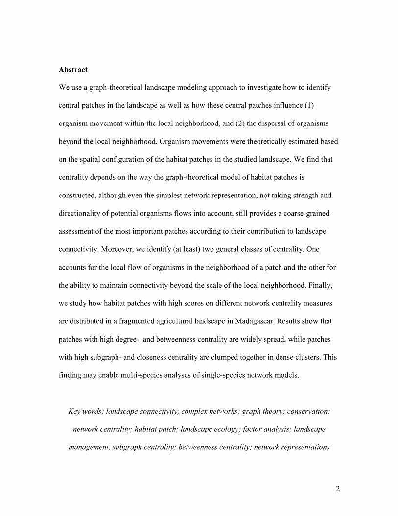
Abstract

We use a graph-theoretical landscape modeling approach to investigate how to identify

central patches in the landscape as well as how these central patches influence (1)

organism movement within the local neighborhood, and (2) the dispersal of organisms

beyond the local neighborhood. Organism movements were theoretically estimated based

on the spatial configuration of the habitat patches in the studied landscape. We find that

centrality depends on the way the graph-theoretical model of habitat patches is

constructed, although even the simplest network representation, not taking strength and

directionality of potential organisms flows into account, still provides a coarse-grained

assessment of the most important patches according to their contribution to landscape

connectivity. Moreover, we identify (at least) two general classes of centrality. One

accounts for the local flow of organisms in the neighborhood of a patch and the other for

the ability to maintain connectivity beyond the scale of the local neighborhood. Finally,

we study how habitat patches with high scores on different network centrality measures

are distributed in a fragmented agricultural landscape in Madagascar. Results show that

patches with high degree-, and betweenness centrality are widely spread, while patches

with high subgraph- and closeness centrality are clumped together in dense clusters. This

finding may enable multi-species analyses of single-species network models.

Key words: landscape connectivity, complex networks; graph theory; conservation;

network centrality; habitat patch; landscape ecology; factor analysis; landscape

management, subgraph centrality; betweenness centrality; network representations

3

INTRODUCTION

Habitat loss, as a consequence of increased human land use and expropriations of

natural habitats, is increasingly being considered as one of the major threats to

biodiversity and functional ecosystems (Meffe et al. 2002, Fahrig 2003). Habitat loss

basically gives rise to two different, although closely related, spatial consequences. First,

the amount of natural habitat obviously decreases as more land is converted for expample

agricultural production. Secondly, the conversion of natural habitat decreases the

connectivity of the landscape, i.e.,, it increases the level of habitat fragmentation. The

focus of this paper is on this latter consequence of habitat loss. Connectivity is, on a

general level, the degree to which the spatial pattern of scattered habitat patches in the

landscape facilitates or impedes the movement of organisms (Taylor et al. 1993). The

persistence of spatially-structured species populations ― metapopulations ― is strongly

related to the connectivity of the landscape (Hanski and Ovaskainen 2003). If the

connectivity of the landscape is too low, subpopulations get isolated, and for instance the

possibility of recoveries following local extinctions decreases since successful

recolonization is dependent on the dispersal of species throughout the landscape (Hanski

and Ovaskainen 2003, Hanski 1994, Bascompte and Solé 1996). On the other hand, even

if habitat fragmentation has decreased the number of large coherent patches of habitat in

the landscape, a sufficiently high level of connectivity may still provide for sufficiently

large areas of reachable habitat, as seen by species capable of moving from patch to patch

(Lundberg and Moberg 2003). Thus, management and planning should take these, and

other, aspects of landscape connectivity into account in order to provide ecologically

functional and resilient landscapes in for instance, designing natural reserves and in green

4

area planning of urban and/or semi-urban areas (Bengtsson et al. 2003, Lee and

Thompson 2005, Bodin and Norberg 2007). Within this problem domain of management,

one of the challenges is to differentiate the impact individual habitat patches have on the

overall connectivity of the fragmented landscape. Often, not all natural habitats can be

preserved since a multitude of different societal interests in land usages has to be

balanced in a typical management situation (Bengtsson et al. 2003). The problem that not

all habitat patches can be preserved begs the question; Which ones shall managers choose

to conserve? Furthermore, the flip-side of that question is; Which patches can be

exploited while still minimizing the negative ecological consequences?

At present there is an abundance of metrics that quantify landscape pattern

(Gustafson 1998), but how well these metrics explain ecological processes is still largely

unknown (Hargis et al. 1998, Tischendorf 2001). Ecological interpretability is however of

crucial importance for any spatial configuration metric in order to make it useful in

management (Li and Wu 2004). One promising approach fulfilling this criterion is the

graph-theoretical perspective on landscape connectivity (Keitt et al. 1997, Urban and

Keitt 2001, Pascual-Hortal and Saura 2006, Bodin and Norberg 2007, Campbell Grant et

al. 2007, Minor and Urban 2007, Calabrese and Fagan 2004). This approach merges

population processes, such as dispersal, with spatial patterns of habitat patches - on the

level of landscapes - in order to attain process-based measures of connectivity (Urban and

Keitt 2001). The basic idea is to depict landscapes of fragmented habitat patches as

networks where the patches are the nodes and the links are the possible dispersal

pathways for dispersing species.

5

For this study, our focus is to elaborate on different methods, using the graph-

theoretical modeling approach to landscape connectivity, to assess and differentiate the

importance of individual habitat patches in relation to their impact on different aspects of

the landscape’s connectivity (Pascual-Hortal and Saura 2006). Within the broad

interdisciplinary field of network analysis, the concept of centrality is used to assess the

individual capability of nodes to influence others (Wasserman and Faust 1994, Estrada

2007a). In short, the concept of centrality is manifested through a family of network-

centric metrics designed to assess, broadly defined, individual nodes’ level of influence

based on their structural position relative to others in the network. Our detailed objective

with this study is to examine the applicability of a range of such centrality measures in

studying individual habitat patches contribution to the landscape connectivity. The goal is

to develop methods helpful in real world situations where management needs to make

informed decisions on which habitat patches to conserve, and which ones to exploit. The

current work also connects to the evolving field of network-oriented studies of different

complex systems ranging from social and technological to biological and ecological

(Strogatz, 1998; Albert and Barabási, 2002; Newman, 2003; Boccaletti et al. 2006).

Here we first briefly present a heavily fragmented agricultural landscape in southern

Madagascar (Bodin et al. 2006) which is thereafter used throughout the paper for the

different analyses. We proceed with presenting some different approaches in constructing

network representations of highly fragmented landscapes, followed by a presentation of a

selected set of centrality measures. Then, by applying these different network

representations on the Madagascar landscape, we examine (1) how the selected set of

centrality measures behave in relation to these different kinds of network representations,

6

and (2) how the centrality measures differ among each other. We show that these

measures, on a general level, can be reduced to two different aspects of centrality, both of

potentially great importance in assessing individual patches’ contributions to landscapes

connectivity. These aspects are suggested to encompass (1) a patch’s contribution to the

magnitude of species interpatch movements on a local geographical level, and (2) the

criticality of an individual patch when it comes to providing large-scale connectivity,

i.e.,, the importance of the individual patch in preventing the network of habitat patches

to divide into smaller and isolated compartments, or islands, of patches. Finally we

present an analysis of the geographical distribution of the patches with high scores on

different measures of centrality, and suggest a multi-species analysis using species-

specific network representations of fragmented landscapes.

METHODS

Study area – southern Madagascar

The study area used throughout the analyses in this paper is located in the Androy

region in the very south of Madagascar, and it is described in details elsewhere (Bodin et

al. 2006; Bodin and Norberg 2007). It consists of hundreds of small forest patches (<1 to

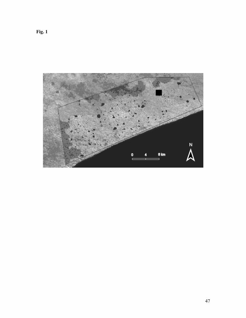
95 ha) that are scattered in an agricultural landscape (Fig. 1). This study area was chosen

since it provides an illustrative example of a landscape that has been fragmented as a

result of agriculture. In spite of its limited size, the forest patches provide habitat for our

target species; the Ring-tailed Lemur (Lemur catta). L. catta is an important seed

disperser in the area since it forages on fruits of many different plant species in the area

(see Bodin et al. 2006 and references therein). Hence their movement between different

forest patches, and in the matrix, can potentially disperse seeds throughout the landscape

7

and accordingly it may contribute significantly to this important ecosystem service

(Millennium Ecosystem Assessment 2003). A spatial analysis of the fragmented forest

patches, as experienced by L. catta, is therefore of interest in order to gain insights in

how well the landscape’s spatial configuration supports seed dispersal. In this study, we

build on a previous graph-theoretical analysis of how L. catta may experience the studied

landscape; thus details on assessments of movement capability and habitat suitability are

not included here but can be found in Bodin et. al. (2006).

Insert Fig. 1 about here.

Graph representations of fragmented landscape

The basic modeling approach in this paper is to present a landscape of scattered

habitat patches as a network consisting of nodes and links (Keith et al. 1997). Each

habitat patch is here represented as a node, and a link between any two nodes represents

connectivity between the two corresponding patches. If two patches are connected, the

target species is able to move between these patches thus implying there is a potential

flow of organisms between the two. There are a number of different methods available to

estimate the level of connectivity between any two patches (Keitt et al. 1997, Bunn et al.

2000, Verbeylen 2003, Bodin et al. 2006). These methods represent different ways of

quantifying the effective distance, as experienced by the target species, between the

patches in question. In its simplest form, the effective distance will be the same as the

geographical distance. In heterogeneous landscapes, the effective distance between any

two patches should be assessed based on the permeability of the specific land types

separating these. In any case, longer effective distance means less connectivity (and flow

of organisms) between the patches. In this study, we estimated the flow of organisms

between any two patches by applying the underlying assumptions behind the Incident

8

Function Model (Hanski 1994). Thus, the flow was assumed to decrease exponentially

with increasing inter-patch distance and to increase proportionally to the square root of

the habitat patch area (see further details in Bodin et al. 2006).

After assessing the connectivity between all pairs of patches in the landscape, the

resulting network will represent all possible movement paths throughout the landscape,

i.e.,, it will represent the landscape’s structure of connectivity as experienced by the

target species.

In general, a network of fragmented patches is represented as a NxN matrix, called

an adjacency matrix A where each patch (of a total of N patches) is represented by one

row and one column (Harary 1969). Then, each element ijA represents the level of

connectivity between patch i and patch j . The most general representation of a

landscape network is a so-called weighted directed graph, where each element in A is

weighted and ijA is not necessarily the same as jiA (Harary 1969). This representation is

often simplified by dichotomizing all elements based on a threshold weight, and the

adjacency matrix can also be made undirected ( ijA equals jiA ). These different

representations are described below.

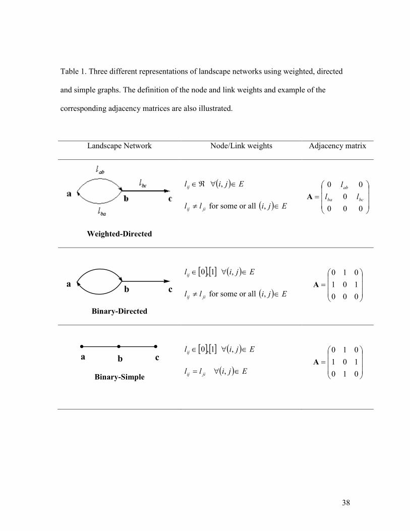
i) Weighted-directed network. In this representation the weight of the network links are

proportional to an estimated flow of organisms potentially moving from one patch i to

another patch j as explained earlier. Obviously, the number of organisms flowing from

i to j are not necessarily the same as those flowing in the reverse direction. Thus, the

network is directed and its adjacency matrix is asymmetric. The adjacency matrix, A for

9

this network is a squared non-symmetric matrix whose elements ijA are defined as

follows:

= equals if 0

weight having to fromlink a is thereif ji

lj ilA ijij

ij (1)

ii) Un-weighted directed networks. This is a simplified representation of the weighted-

directed network in which no link weight is quantified but we still consider the direction

of the links joining the nodes. There is a link from patch i to j if there is a potential flow

of organisms in this direction which exceeds a predefined threshold value (Bodin et al.

2006). This network is represented by a binary directed graph where the weight ijl is 1 if

there is a link from node i to node j , or 0 otherwise. The elements of the asymmetric

adjacency matrix are thus defined as follows

= otherwise 0

to fromlink a is thereif 1 j iAij (2)

iii) Un-weighted undirected networks. The simplest representation of a landscape

network is the un-weighted undirected graph. In this case we consider two nodes as

connected if there is a connection between the corresponding patches irrespectively of its

direction. The link weights are 1 or 0 if the corresponding nodes are connected by a link

or not, respectively. Thus, the adjacency matrix is a binary symmetric matrix whose

elements are defined as follows:

= otherwise 0 to fromor to fromlink a is thereif 1 i j ji

Aij (3)

In Table 1 we illustrate the three types of landscape network representations and

their respective adjacency matrices.

Insert Table 1 about here

10

“Classical” network centrality measures

Here we present some centrality measures used in studying various different kind of

networked systems (Costa et al. 2007, Jordán et al. 2007, Wasserman and Faust 1994).

i) Degree centrality ( )iDC , is simply the number of links of a node i, i.e.,, the

number of patches that have a functional connection from or to the patch i. In a directed

network we will distinguish two types of degree centralities: in-degree and out-degree

centralities. The in-degree centrality ( )iDCin is the number of links which terminate in

patch i in the landscape. The out-degree centrality ( )iDCout is the number of links that

originate from the patch i (Harary 1969). If a landscape has link weights then the in- and

out-degree centralities are calculated by summing up the link weights for all the links

terminating or originating, respectively, at the corresponding patch.

ii) Betweenness centrality BC(k) is defined as the fraction of shortest paths going

through a given node k . If ( )ji,ρ is the number of shortest paths from node i to node j,

and ( )jki ,,ρ is the number of these shortest paths that pass through node k in the

network, then the betweenness centrality of node k is given by (Wasserman and Faust

1994; Freeman 1978):

( ) ( )( ) kji

jijkikBC

i j≠≠

ρρ

=∑∑ ,,,,

(4)

In weighted networks the shortest paths could be defined as the sum of the link weights.

iii) Closeness centrality ( )iCC is the sum of the distances from node i to all other

nodes in the network, where the distance ( )jid , is defined as the number of links in the

shortest path from node i to node j. The closeness centrality of node i is given by the

following expression (Wasserman and Faust 1994; Freeman 1978):

11

( ) ( )∑−

=

jjid

NiCC,1 (5)

In weighted networks the distance could be defined as the sum of the link weights. The

closeness centrality cannot be calculated for all patches in a disconnected landscape

because the distance between un-connected patches is infinite or just undefined.

iv) Eigenvector centrality EC(i) was introduced by Bonacich (1972, 1987) and is

defined using the principal eigenvector of the adjacency matrix A. EC(i) of node i is

defined as the ith component of the eigenvector 1e that corresponds to the largest

eigenvalue of A (principal eigenvalue):

( ) ( )ieiEC 1= (6)

The eigenvector centrality has some limitations when applied to the different types

of network representations previously presented (Borgatti and Everett 2006). First, it

cannot, in its original form, be unambiguously defined for directed networks.

Furthermore, it assigns zeros to all patches which are not situated in the largest

component (i.e., a subset of nodes where there exist a path between each and every pair

of nodes) of the network even if they are highly central in their respective components

(Borgatti and Everett 2006).

Subgraph centrality

One of the authors (EE) has recently introduced a metric characterizing certain

aspects of importance of a node in a network which is named the “subgraph centrality”

( )iSC (Estrada and Rodríguez-Velázquez 2005). This metric characterizes the

participation of a node in all structural motifs (e.g., triangles, squares, etc.) in the

network. The participation of a node in a motif is quantified by means of the so-called

12

closed-walks (CWs). A walk of length r is a sequence of nodes 121 ,,,, +rr vvvv such that

for each ri ,2,1 = there is a path from iv to 1+iv . A closed walk (CW) is a walk in

which 11 vvr =+ (Harary 1969). A particular case of CW is the cycle, in which all nodes in

121 ,,,, +rr vvvv are different, but in general a closed walk can involve the same node

more than once. In a network representation of a fragmented landscape, these CWs

represent different movement pathways within the landscape that terminates at the

originating patch.

If we consider a particular node i , the total number of CWs of length r originating

(and terminating) at i is designated by ( )irµ . The general idea behind the subgraph

centrality measure is to relate a node’s centrality to the number of CWs of different

lengths starting at a given node. However, the sum of CWs of all lengths starting and

ending at a given node is infinite, i.e.,, ( ) ∞=∑∞

=0rr iµ , which would makes this measure

useless. This difficulty is resolved by introducing a weighting scheme that makes that the

sum of weighted CWs converge to a definite value (Estrada and Rodríguez-Velázquez

2005).

( ) ( ) ( )∑ ∑∞

=

∞

=

==0 0 !!r r

iir

r

rriiSC

Aµ (7)

Thus, a CW of length two is weighted by a factor of ½, and a CW of length three is

weighted by a factor of 1/6 and so on. In general, a CW of length r is weighted by a

factor of !/1 r , which makes the sum of weighted CWs converge, and also fulfill the

intuition that the longer closed walks are of less importance in defining a nodes level of

centrality (see further explanations in Estrada and Rodríguez-Velázquez 2005).

13

For practical reasons we need to truncate the infinite sum given by expression (7).

In doing so we will stop the calculation for the value of r such that

410!

−≤r

rµ (8)

Furthermore, in a binary and undirected representation of a network, (7) converges

to the following expression:

( ) ( )[ ] jeir

iSCN

jj

r

r λγµ 2

10 ! ∑∑=

∞

=

== (9)

where ( )ijγ is the ith component of the jth eigenvector of the adjacency matrix A and jλ

is the corresponding jth eigenvalue (Estrada and Rodríguez-Velázquez, 2005).

Finally, as seen from an ecological perspective, if a patch in a landscape has a large

subgraph centrality, a species would be able to move from that particular patch to a large

number of other patches - and then return - by using predominantly closed walks of small

lengths.

Centrality measure correlations

Of interest is to examine to what extent the different centrality measures capture

certain distinct aspects of the patches’ structural positions, and to what extent the

different measures overlap (correlate) in this regard. Furthermore, it is of interest to study

to what extent the different centrality measures depend on the different networks

representations described earlier. In order to enable such analysis, we calculated the in-

and out-degree, the betweenness, the in- and out-closeness and the subgraph centrality for

all nodes, in all types of network representations, and correlated the resulting values for

all centrality measures for all nodes. Hence, we (1) tested the degree of correlation

14

between the values for the different centralities for each network representation, and we

(2) correlated the centralities among the three different types of network representations.

In addition to the centrality measures mentioned above we also calculated the

eigenvector centrality for the simple graph representation of the network, which has a

symmetric adjacency matrix allowing such calculations.

Furthermore, to examine to what extent the different centrality measures overlapped

we use the principal component (PC) method (Gorsuch 1983) to reduce the six-

dimensional centrality space as much as possible while still accounting for most of the

variance of the centrality measures. In order to obtain a clear pattern of loadings we will

use a typical strategy known as Varimax, which rotates the factors in an orthogonal way

(Gorsuch 1983).

Clumpiness coefficient

A network characteristic that has received fairly little attention is how close to each

other the most central nodes in a network are. We believe that such characteristics could,

however, be of particular interest in studying some aspects of a landscape’s spatial

configuration. If for instence, a set of patches, each with high degree centralities, are also

directly connected to each other, one might expect a high degree of organism movements

confined within such a set.

One measure that tries to capture this network characteristic is the assortativeness

introduced by Newman (2002). This measure quantifies whether the most connected

nodes in a network are connected to each other or to the least connected ones. Newman

proposed measuring the Pearson correlation coefficient of the degree-degree correlation

to quantify the assortativeness (Newman 2002). However, this measure only takes into

15

account the pairs of connected nodes and does not say anything about the pairs of nodes

separated at topological distance larger than one. In order to include these pair of nodes in

the analysis we here define a clumpiness coefficient ( )CΛ for the centrality measure C .

The clumpiness coefficient is defined as the averaged value of the product of the

standardized centrality for all pairs of nodes jiCC ˆˆ in the network divided by the square

of the corresponding topological distance ijd separating them,

( ) ( )∑<

=ΛN

ji ij

ji

d

CCC 2

ˆˆ (10)

The standardization of the centralities is carried out by s

CCC i

i

−=ˆ , where C is

the average and s is the standard deviation of the centrality. This standardization

guarantees that we can compare centrality measures which have very different values as

they have an average value of zero and standard deviation of one. As can be seen from

this expression, when the most central nodes are directly connected, 1=ijd , the

clumpiness reaches its maximum. However, when the most central nodes are far away

from each other, 1>>ijd , the clumpiness is reaching its minimum. Here we are using the

topological distance between the pairs of nodes but in other cases the topological distance

ijd could be replaced by the effective distance (i.e., the link weights) separating the

patches in order to obtain a clumpiness estimate of a centrality measure taking the

effective distances into account.

Expression (10) can be obtained from a direct vector-matrix-vector multiplication

procedure (Estrada, et al. 1997; Estrada and Rodríguez 1997). Let c be a column vector

16

of the standardized centrality measures and R the matrix of reverse squared distances

between pairs of nodes in the graph. Then the clumpiness coefficient is obtained by,

( ) ( )TC cRc21

=Λ (11)

where T stands for the transpose of the vector. Some generalizations and statistical-

mechanics interpretation of the clumpiness coefficient have been recently published by

Estrada et al. (2008).

Simulation of patch losses

Ultimately, our interest in the different centrality measures lies in their ability to

assess the contribution of a patch to various aspects of the connectivity of a fragmented

landscape. In this study we estimated this ability by simulating the removal of patches,

ten-by-ten, starting with the most central nodes according to different centrality

measures. This strategy has been applied previously to different kinds of complex

networks (Estrada 2006; Estrada 2007b). We selected two different network descriptors

to assess the centrality measures’ abilities to identify patches that characterize the

landscape network as a whole. First, we analyzed how the network cliquishness is

affected by the removal of the patches. By cliquishness we mean to what extent links tend

to be distributed to certain well-connected sets (cliques) of nodes, or if just distributed

randomly. High cliquishness would imply high local neighborhood connectivity. In a

heavily fragmented landscape, high local connectivity implies access to a fair amount of

nearby habitat patches thus providing home ranges of sufficient sizes (cf. Bodin et al.

2006). As a cliquishness measure we selected the Watts-Strogatz clustering coefficient,

which is defined as (Watts and Strogatz 1998)

17

iiCi nodeon centered triplesofnumber node toconnected trianglesofnumber

= (12)

The second parameter to be considered is the size of the largest component. If the

size of the largest component (in terms of the number of patches it contains) is big in

comparison to the total number of patches in the landscape, the level of connectivity can

be interpreted as high.

RESULTS

Weighted directional Madagascar network

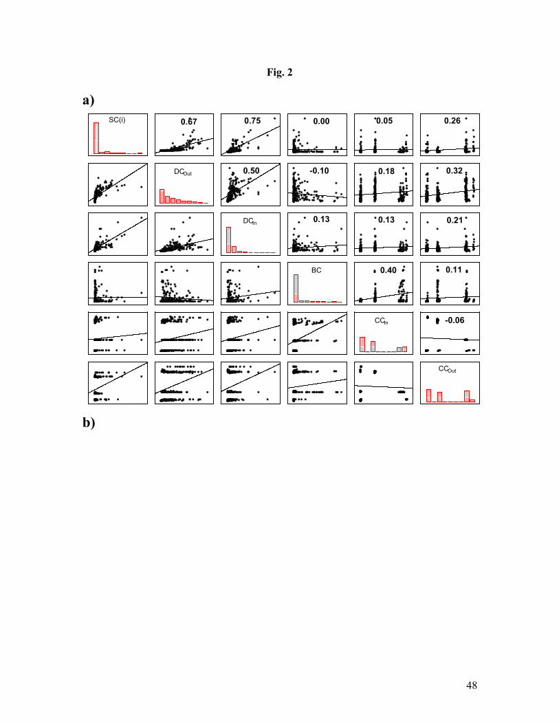
In Fig. 2A we show, for every patch, the intercorrelations between every pair of the

centrality measures studied of the weighted directional version of the Madagascar

landscape network. The most evident characteristic that can be observed in this plot is the

generally low level of correlation between many of the pairs of centrality measures. This

clearly shows that different centrality measures are ranking the nodes according to

different criteria. The most correlated centralities are the subgraph centrality and the

degree centralities, which all show some linear interdependence among each other. On

the other extreme we find the closeness centralities, which are not well correlated with

neither of the other measures. The differences in the criteria of centrality measures are

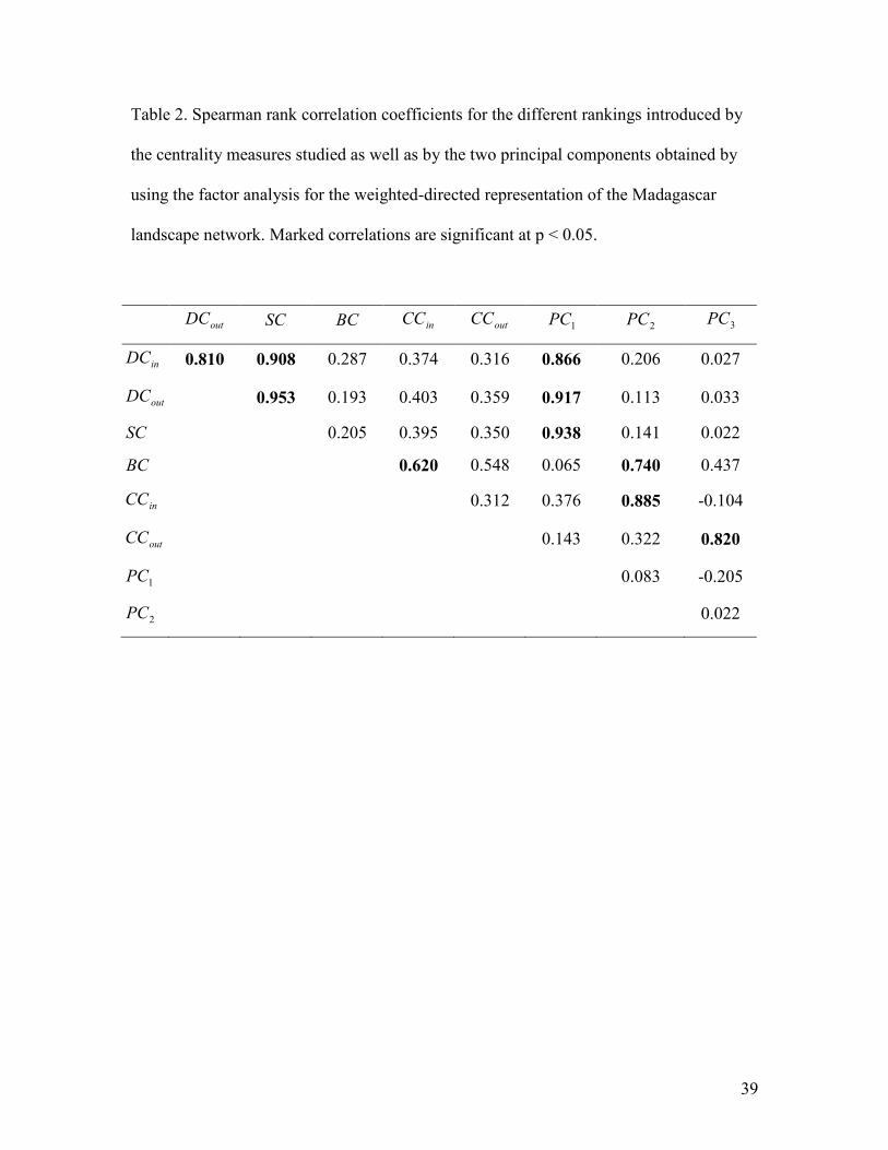
reflected in the ordering of the patches according to their centrality scores. In Table 2 we

give the Spearman correlation coefficients for the different rankings introduced by these

centrality measures. These statistics represent the relationship between different rankings

on the same set of patches. That is, these coefficients measure the correspondence

between two rankings, and assess the significance of this correspondence. If two rankings

are the same the Spearman coefficient is equal to 1 and if one ranking is the reverse of the

other the coefficient has the value –1. In general, this coefficient lies between –1 and 1,

18

and increasing absolute values imply increasing agreement between the rankings. As can

be seen in Table 2 most of the values of the Spearman correlation coefficient indicate that

there is a poor correlation between the different rankings. The best agreements are

obtained between the subgraph centrality and the degree centralities. These different

rankings beg the question of how to obtain a relevant global ranking of the overall level

of centrality of nodes in a landscape network.

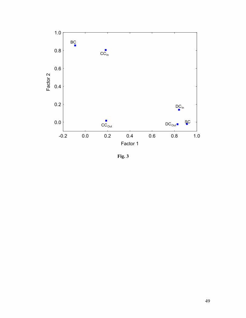
Using the principal component (PC) method we have been able to reduce the six-

dimensional centrality space to three dimensions where three principal components ( 1PC ,

2PC and 3PC ) account for 80% of the variance of the centrality measures. There are

three centrality measures that load in 1PC (the two degree centralities and the subgraph

centrality). 2PC accounts for the betweenness and in-closeness centralities and 3PC only

accounts for the out-closeness centrality. We have then carried out a Varimax rotation

(Gorsuch 1983) to orthogonalize the principal components and obtain their structural

interpretation. In Fig. 2B we plot the first two components ( 1PC and 2PC ) after this

rotation. The two degree centralities and the subgraph centrality have positive

contributions to 1PC . Since the degree centralities measure the number of functional

connections (i.e., links) with the surrounding patches, and subgraph centrality measures

the level of participation of a patch in structural motifs like triangles, squares, etc, PC1

can be interpreted as a measure of the total dispersal of organisms through the

corresponding patch.

On the other hand, the second principal component is dominated by the

betweenness centrality and in-degree closeness centrality. Patches with high scores of the

betweenness centrality have previously been shown to help bring together otherwise

19

largely separated groups of patches (Bodin & Norberg 2007). If these “bridging” patches,

also known as cutnodes, are removed, the connected landscape would risk being

separated into significantly smaller compartments (which our experiments of node

removals presented further on also confirm). Consequently, the principal

component 2PC , can be understood as a measure of the corresponding contribution of a

patch in upholding the large-scale connectivity of the landscape. In Table 2 we have

included the Spearman rank correlation coefficients for the three principal components. It

can be seen that the ranking introduced by 1PC agrees very well with the rankings

introduced by the degree and subgraph centrality. The highest coefficient is obtained for

the subgraph centrality. The ordering introduced by 2PC correlates very well with the

ranking introduced by the in-closeness centrality and the betweenness centrality and the

ordering introduced by 3PC agrees with the one introduced by the out-closeness

centrality.

Insert Table 2 and Fig. 2 about here.

Unweighted (binary) directional Madagascar network

We calculate the centrality measures for all nodes and obtain the inter-centrality

correlations, which are illustrated in Fig. 3. Betweenness and closeness centralities are

exactly the same as for the weighted version of the network as we did not consider the

link-weights in these calculations. As can be seen there is, again, a generally low level of

correlation between many of the pairs of centrality measures. However, the correlation

between the degree centralities is significantly higher for the binary-directed than for the

weighted directed network.

20

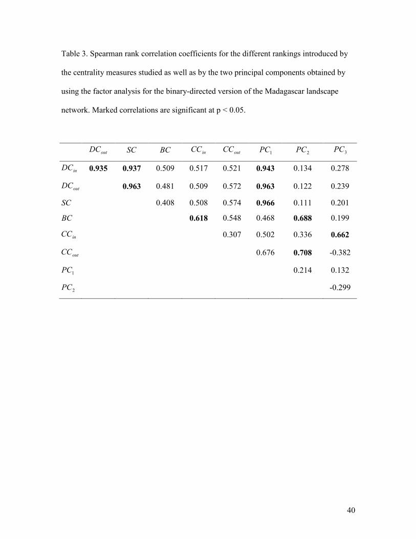
When analyzing the Spearman rank correlations between the centrality measures we

can observe (see Table 3) that there is a high level of correlation between the rankings

introduced by degree centralities and subgraph centrality. The other two rankings which

are in some way correlated are the ones introduced by in-closeness and betweenness

centralities.

Insert Fig. 3 about here.

The factor analysis revealed three principal components accounting for 88% of the

variance of the original centrality measures. As in the previous case the first principal

component, 1PC is described by the degree and subgraph centralities. The second factor

2PC is represented only by the betweenness centrality. Thus, the interpretation of these

factors is the same as before. In Table 3 we can see that there are high rank correlations

between the 1PC and the two degree centralities as well as subgraph centrality. As

before, the second principal component is rank correlated to the betweenness but in this

case also with the out-closeness centrality instead of the in-closeness centrality.

Insert Table 3 about here.

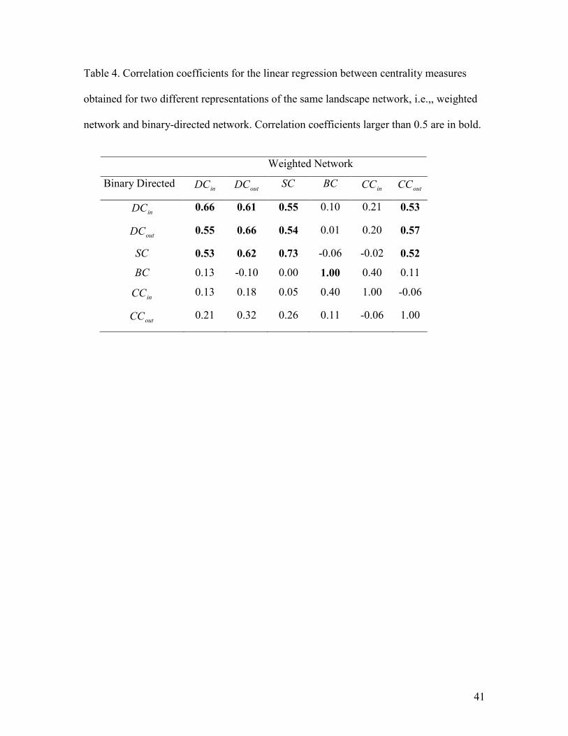
In Table 4 we show how the centrality scores calculated for the weighted version

correlate with the scores calculated for the binary version of the network representation.

By analyzing the diagonal entries of the table, it is possible to compare the same

centrality measure of the two network representations of the landscape. As can be seen

the subgraph and the degree centralities are fairly correlated (correlation coefficient=0,73

and 0,66), but some information is obviously lost when the link weights are omitted from

the analysis (cf. Scotti et al. 2007). For example, only 50% of the patches in the 1PC top

ten coincide for both types of networks (data not shown). Betweenness and closeness

21

centrality were calculated without taking link weights into account, thus their correlation

coefficients are 1.

Insert Table 4 about here.

Binary undirected network

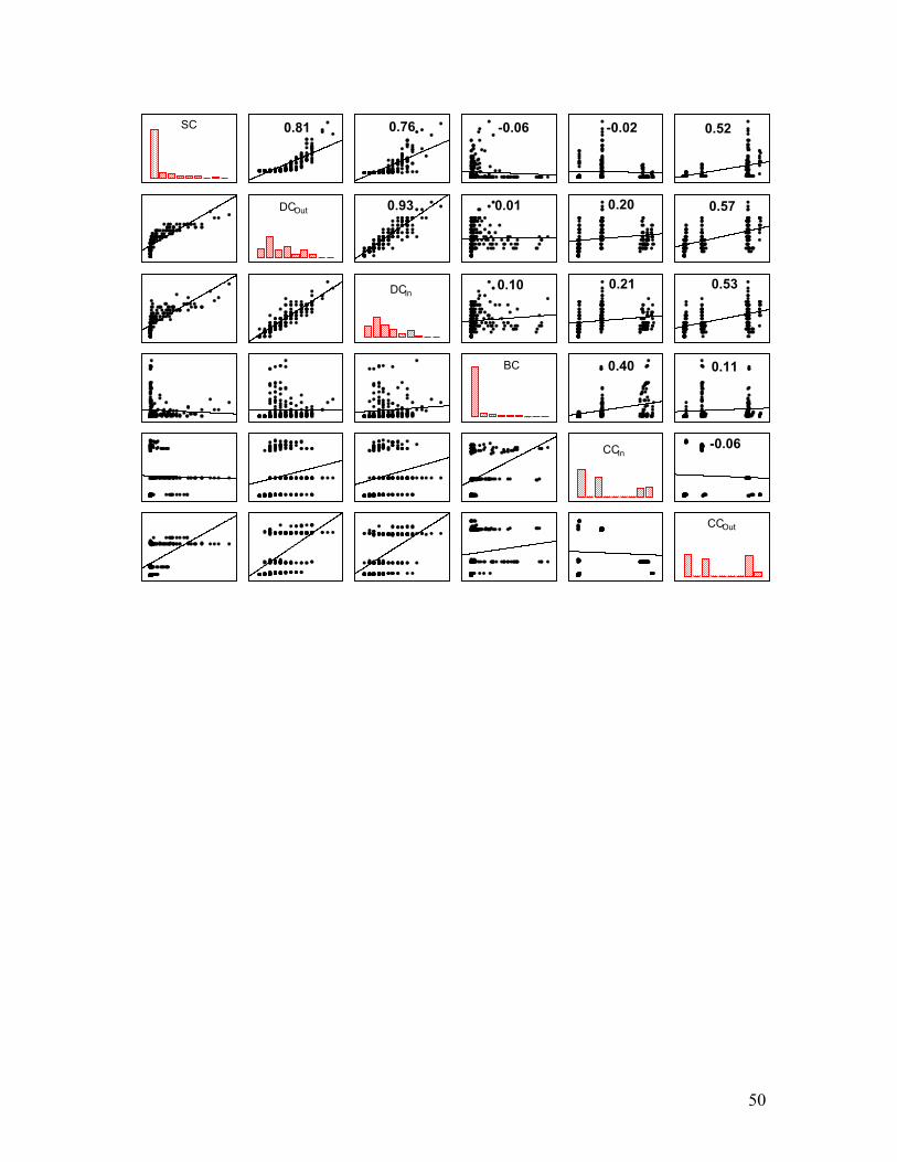
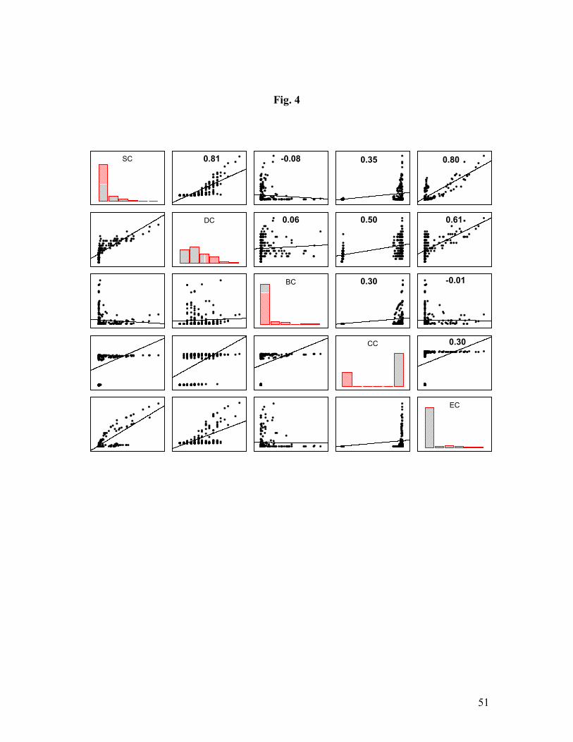
In Fig. 4 we illustrate the correlation between every pair of centrality measures in

this simple graph representation of the Madagascar landscape. As before there is a low

level of correlation between many of the pairs of centrality measures. However, the

subgraph and degree centralities display some correlations, as do the subgraph and

eigenvector centralities. In the latter case the correlation is significantly reduced by the

fact that eigenvector centrality assigns zero centrality for all patches which are not within

the largest connected component of the network.

Insert Figure 4 about here.

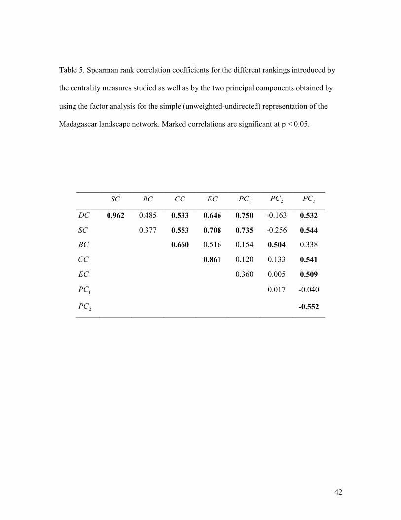
In Table 5 we give the Spearman correlation coefficient for the different rankings of

patches according to the centrality measures analyzed. There is a large coincidence in the

rankings introduced by degree, subgraph and eigenvector centrality. Surprisingly, the

eigenvector centrality introduces a ranking of patches which is highly correlated to the

one introduced by the closeness centrality. The ranking introduced by the betweenness

centrality is very unique as it does not correlate with any of the other rankings. A factor

analysis identifies a principal component in which degree, eigenvector and subgraph

centralities are highly loaded. The second principal component accounts for the

betweenness and the third for the closeness. Hence, it is apparent that there are large

similarities in the reduced centrality spaces obtained for the three different network

representations. The ranking obtained by using 1PC , 2PC and 3PC are also given in

Table 5. The first two principal components continue having similar rankings as the

22

centrality measures scored in such factors. The third principal component, however, has

high Spearman correlation coefficients with most of the centrality measures.

Insert Table 5 about here.

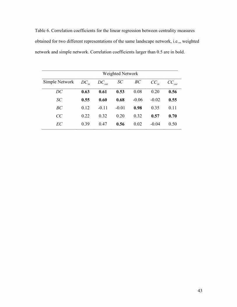
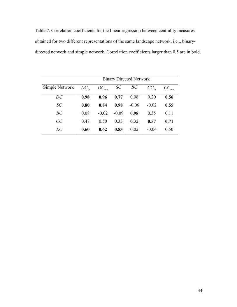
Table 6 and 7 present the correlations between centralities of patches for the three

different network representations of the landscape. The degree of correlation between

degree and subgraph centrality is for example slightly reduced when correlating the

simple network with the weighted directed one than when correlating the weighted-

directed one with the binary directed network. Overall, as before, the level of correlation

remains fairly low.

Insert Table 6 and 7 about here.

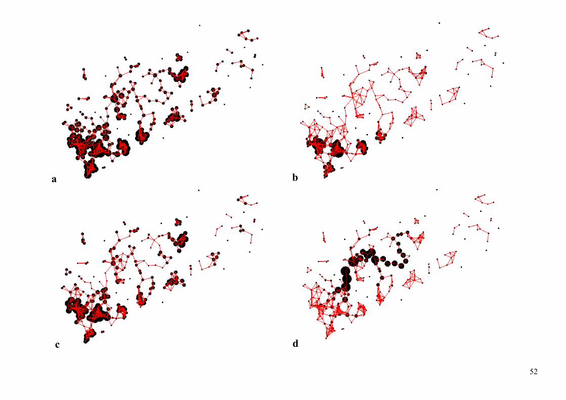
How are central patches distributed across the landscape?

In Fig. 5 we illustrate how the patches with the highest scores of the degree,

betweenness, closeness and subgraph centralities for the simple network representation of

the Madagascar landscape are distributed. The sizes of the nodes are proportional to the

value of the centralities. As can be seen in Figure 5 the most central nodes according to

the degree and the betweenness measures are spread across the network. However, the

most central nodes according to the subgraph centrality form very compact clusters,

which are localized in small regions of the landscape.

If we calculate the clumpiness coefficients for the degree, betweenness, closeness

and subgraph centralities of the Madagascar network we confirm quantitatively our

observation that subgraph centrality is more clumped than degree centrality in this

network, ( ) 09.634=Λ SC and ( ) 30.438=Λ DC . Also, in this landscape the betweenness

centrality has a small clumpiness, ( ) 09.225=Λ BC , which confirms that most of the

bridges/cutpoints in the network are spread across the landscape and are not concentrated

23

in small regions. By definition the closeness centrality should be the most clumped

centrality as it is conceptualized to give higher weight to the nodes which are close to

other nodes. In fact, ( ) 92.732=Λ CC .

Insert Figure 5 about here

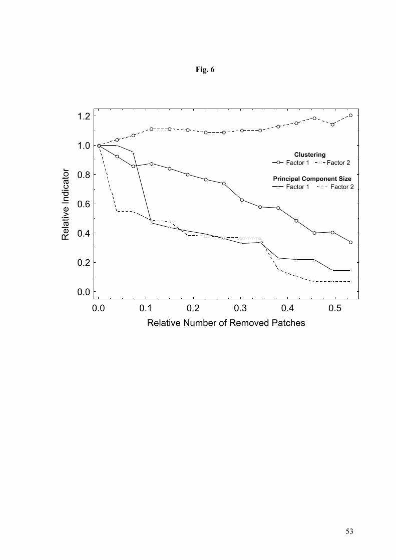
Vulnerability to patch loss

Here we simulate how the Madagascar landscape might be affected by the loss of

patches. The objective of the simulation is to assess how the loss of the most central

patches identified by the different centrality measures affects aspects of the network

topology, with consequences on the ecological processes in the landscape. As previously

described we selected the most complete description of the Madagascar network for the

simulation, which is the weighted directed network. We removed the patches, ten-by-ten,

according to their values of the two principal factors identified previously.

The original network is formed by 29 components, which are by definition not

connected to each other. In Fig. 6 we present the results of the simulation, where the x -

axis represents the relative number of patches removed and the y -axis represents the

relative value of the indicator used. The relative indicators are calculated by dividing the

value of the indicator for the disturbed network by that of the original network. By using

continuous line we represent the effects produced by the removal of the most central

patches according to the PC1, i.e.,, the one we propose as representing organism

dispersal, while a discontinuous line represents the effects produced by the removal of

patches according to factor PC2, i.e., the one we propose as representing the contribution

of a patch in upholding the large-scale connectivity. If we consider the network

cliquishness (local neighbourhood connectivity) we can see that this parameter is almost

24

unaffected when the most central patches ranked by factor PC2 are removed. However,

the removal of the patches according to the factor PC1 produces a dramatic reduction of

the cliquishness of the network and by removing about 40% of patches the cliquishness is

reduced by 50%.

The size of the largest component of the network is reduced from 173 patches to

only 95 when the 10 most central patches according to factor PC2 are removed. The

number of patches, however, remains high for the removals based on the PC1. The

elimination of the top 20 patches according to PC1 only reduces the size of the largest

component from 173 to 165 patches. However, after 10% of nodes are removed both

factors predict approximately the same effect on the size of the principal component. This

somewhat unexpected behavior is mostly a consequence of the severe fragmentation of

the principal component following the first removals. Thus, continued patch removals are

based on centrality scores which are no longer relevant, therefore it is not surprising that

the difference between the two removal schemes is so small.

Insert Fig. 7 about here.

DISCUSSION

Two families of network centrality

By comparing the results of the analyses of the different centrality measures in the

three different network representations of a fragmented landscape (weighted-directional,

unweigthed-directional and unweighted-undirectional) we observed the following

generalities described below.

(1) There are (at least) two distinct types (families) of centralities among the set of

selected centrality measures for the network studied here. We interpret the first type as

potentially relevant in estimating organisms’ dispersal at the level of the local

25

neighborhood, and the other type as relevant in estimating the ability of individual

patches to maintain connectivity beyond the scale of the local neighborhood. The first

type includes (in/out) degree-, eigenvector- and subgraph centrality and the second type

includes the betweenness centrality for all cases. The simulation of patch removal

confirmed the aforementioned differences between the two types of centralities.

(2) These two families of network centrality remain distinct for all three types of

network representations. This assessment resulted from the factor analyses of all three

network representations where the different centrality measures listed above always

ended up in the same principal components, irrespectively of the type of network

representation. The closeness centrality, on the other hand, did not show such

consistency.

(3) The different types of network representations have quite a significant effect on

the assessment of the different centrality scores of individual patches, and that effect

seems to be more profound for the family of centrality measures that we interpret as

relevant in assessing localized organism dispersal. This assessment is based mainly on

the fairly low correlation coefficients of the node centralities in the different network

representations. The information contained in the first principal component, which we

interpret as related to the dispersal of organisms through a given patch, is significantly

affected by the consideration of weight and directionality of links in the landscape

network. In comparison, the second principal component ( 2PC ) is more stable to the

differences in network representation. This difference is, however, partly a consequence

of not considering the link weights for the calculation of the betweenness centrality.

26

(4) Although the different network representations have a profound effect on the

ranking of the individual patches’ centrality scores, most of the higher scoring patches

remain high in centrality irrespectively of the network representation. Thus, even the

simple unweighted and undirected network representation is still useful for a coarse-

grained assessment of individual patches’ importance, but a more detailed assessment of

link strength and direction are clearly preferable.

(5) Since the two different families of network centralities remained the same for all

different types of network representations, it may suffice to use only one centrality

measure from each family for a coarse-grained analysis. Hence, analyses are significantly

simplified while still retaining confidence that no important information is lost.

According to the rank correlation analysis results (Tables 2, 3 and 5) we recommend

using subgraph or degree centrality as a representative of the first principal factor and the

betweenness centrality as a representative measure of the second factor.

To summarize, the two families of centrality measures (i.e., the principal

components 1PC and 2PC ) assessed using six different and widely used centrality

measures, account for two important but distinct aspects of the landscape connectivity.

For instance, the removal of the most central nodes according to 1PC will not separate

the network into more isolated components but will reduce the local neighborhood

connectivity (“cliquishness”) of the network, potentially posing limitations on the

landscape’s ability to attract species with size-requirements on their home range

stretching beyond the size of individual patches. On the other hand, 2PC accounts for the

bridges in the landscape whose removal will separate the landscape into isolated

components. Then, the assessment of whether patches are more central (and thus more

27

important) than others depends on the aspect of landscape connectivity under

consideration. Both aspects of landscape connectivity are important, thus (ideally)

patches scoring high in both families of centralities should be conserved while the

exploitation of other lower-ranking patches may cause less negative impact on landscape

connectivity and its associated ecological processes.

Clumpiness of central patches

As qualitatively revealed in Fig. 5, and quantified using our proposed clumpiness

coefficient, patches with high scores on degree and betweenness centrality are scattered

throughout the whole landscape, whereas patches with high scores on subgraph centrality

are clumped together in distinct and dense clusters of patches. Hence, although there is a

relatively high degree of correlation between subgraph and degree centrality, and despite

the fact that they appear in the same principal component in the factor analysis, there are

clearly some differences between the two. When it comes to the ranking of the most

central patches according to the two measures, there is a high degree of similarity with

Spearman rank correlation coefficients larger than 0.9, irrespective of the network

representation (Table 2, 3 and 5). However, as revealed in Fig. 5, the difference appears

to reside in the ranking of the patches with low to intermediate scores of centrality. All

patches with low to intermediate scores of subgraph centrality are located closely around

the highest scoring patches while for degree centrality this characteristic is far less

pronounced. Here, some of the patches with relatively high degree centrality stand out on

their own, while this never happens for patches with high subgraph centrality.

28

Dense clusters of relatively small patches

In a landscape, in order for a patch to have a high degree centrality, it has to be

located geographically close to many other patches. Thus, due to obvious spatial

constraints, the mean areas of these patches have to be quite small in comparison with the

effective distance the target species can move in the landscape (patches can, by

definition, not overlap; thus in order to fit many patches onto a small area they have to be

small). Furthermore, a particular node’s subgraph centrality score is boosted if its

network neighbors have many neighbors themselves, particularly if these neighbors are

also neighbors to the originating node (and therefore located within reach from the

originating node). This boost is due to the increased number of short-length closed walks

resulting from the well connected local network neighborhood. In order to understand

more formally the relationship between high subgraph centrality and shorter dispersal

distances we exemplify it using an artificial landscape network having n patches in

which every patch is connected to all others in the landscape. This kind of networks

correspond to the so-called complete graphs, nK . We have previously proved

mathematically that the largest subgraph centrality in a network having n nodes is

obtained for the complete graph nK (Estrada and Rodríguez-Velázquez 2005). That is,

among all networks having the same size the maximum subgraph centrality is reached

when all nodes are connected to each other. Of course, this network will also display

most interpatch movements since an organism situated in one patch can reach any other

patch by moving one single step. Similarly, the level of closeness is highest if every node

is connected to every other node. Now, let us consider the network xKn − in which the

link x is removed from nK . Then the number of CWs of length k in xKn − is equal to

29

the number of CWs of length k in nK minus the number of CWs of length k in nK

containing x . Consequently, for all i , ( )iSC in xKn − is lower than ( )iSC in nK . If we

consider that the link x in nK is connecting the patches p and q , then the distance

between p and q in xKn − is increased from 1 to 2. As a consequence, after the

removal of a link in the complete graph the subgraph centrality of any node decreases.

The procedure of link removal can be repeated and the previous assertion can be

generalized. Thus, in general a high subgraph centrality indicates a network

neighborhood that is internally very well connected. In combining this insight with the

previous argument on the relationship between patch sizes and number of neighbors, it

becomes clear that the distinct groups of patches with high subgraph centrality

correspond to areas in the landscape where the habitat has been fragmented into several

small, but well connected and closely located, patches.

A reasonable interpretation of such high density clusters is that the patches within

the clusters are experienced as being connected by species not being able to move as far

in the inhospitable matrix as the target species used to assess the network of fragmented

habitat patches in the first place. This is interesting since one drawback using network

representations of fragmented landscapes is that the assessed networks are, by definition,

specific for the studied target species. If, however, one can use network measures (such

as the subgraph and/or the closeness centrality) to identify core areas that would still

appear as connected for species not being able to move as far as the target species used to

construct the network – a multi-species interpretation of a single species network is

possible.

30

CONCLUSIONS

In order to balance between different socio-economic demands on land use, and still

provide the generation of essential ecosystem services in a fragmented landscape

(Millennium Ecosystem Assessment, 2003; Bodin et al. 2006), there is a need for

scientifically reliable methods capable of identifying individual habitat patches that, more

than other patches, contribute to upholding important aspects of landscape connectivity.

One promising modeling approach that we believe contribute to such development is the

graph-theoretical approach used in this study. Here we have specifically studied how

different measures of network centrality may help to estimate individual patches

contribution to (1) organism movement within the local neighborhood, and (2) the

movement of organisms beyond the local neighborhood. We have studied how these

measures of centrality depend on the way the network of habitat patches is constructed

and thus represented, and we conclude that while the type of network representation have

a profound effect of the assessments of different levels of centrality of patches, even the

simplest network representation, not taking strength and directionality of organisms flows

into account, still provides a coarse-grained assessment of the most important patches

according to the two aforementioned aspects of connectivity.

Furthermore we found a significant difference between the reasonably well-

correlated subgraph and degree centrality measures. Patches with high and intermediate

levels of subgraph centrality are clumped together in the landscape whereas patches with

high to intermediate levels of degree centrality are more scattered. Thus the clumps of

patches with high to intermediate levels of subgrah centrality may be experienced as

connected by other species not being able to move as far in the inhospitable matrix as the

31

target species used to assess the network of fragmented habitat patches in the first place.

This can be seen as a step towards multi-species analyses of networks of fragmented

habitat patches.

Although our results are based on analyses of the specific Madagascar landscape

network, we believe these finding are more broadly applicable since this particular

landscape in Madagascar is not significantly different, as seen from a strictly spatial

perspective, from other heavily fragmented landscapes. Naturally, conducting similar

analyses on a range of different landscapes would be preferable and would strengthen our

arguments. Furthermore, there are other centrality measures not considered here that

might be of relevance in studying landscape connectivity, and there are also reasons to

further examine the underlying assumptions behind these and other centrality measures

when it comes to the kind of flows they might be appropriate for (Borgatti 2005). Finally,

more empirically oriented studies utilizing the graph-theoretical perspective of

fragmented landscapes would also be needed.

ACKNOWLEDGEMENTS

The authors thank Thomas Elmqvist and his co-workers at the Department for Systems

Ecology at Stockholm University for providing access to the Madagascar dataset. E.E.

thanks the “Ramón y Cajal” program, Spain for partial financial support, and ÖB thanks

The Swedish Research Council for Environment, Agricultural Sciences and Spatial

Planning (FORMAS) for financial support. The Swedish Research Council and the

Department for Research Cooperation at the Swedish International Development

Cooperation Agency also provided financial support. The authors thank two anonymous

32

referees for suggestions that significantly improved the presentation of this work.

33

LITERATURE CITED

Albert, R. and A.-L. Barabási. 2002. Statistical mechanics of complex networks. Reviews

of Modern Physics 74:47-97.

Bascompte, J., and R. V. Solé. 1996. Habitat Fragmentation and Extinction Thresholds in

Spatially Explicit Metapopulation Models. Journal of Animal Ecology 65:465-

473.

Bengtsson, J., P. Angelstam, T. Elmqvist, U. Emanuelsson, C. Folke, M. Ihse, F. Moberg,

and M. Nyström. 2003. Reserves, resilience and dynamic landscapes. AMBIO: A

Journal of the Human Environment 32:389–396.

Boccaletti, S., V. Latora, Y. Moreno, M. Chavez, and D.-U. Hwang. 2006. Complex

networks: Structure and dynamics. Physics Reports 424:75-308.

Bodin, Ö., and J. Norberg. 2007. A network approach for analyzing spatially structured

populations in fragmented landscape. Landscape Ecology 22:31-44.

Bodin, Ö., M. Tengö, A. Norman, J. Lundberg, and T. Elmqvist. 2006. The value of

small size: loss of forest patches and ecological thresholds in southern

Madagascar. Ecological Applications 16:440-451.

Bonacich, P. 1972. Factoring and weighting approach to clique identification. Journal of

Mathematical Sociology 2:113-120.

Bonacich, P. 1987. Power and centrality: A family of measures. American Journal of

Sociology 92:1170-1182.

Borgatti, S., and M. G. Everett. 2006. A graph-theoretic perspective on centrality. Social

Networks 28:466-484.

Borgatti, S. 2005. Centrality and network flow. Social Networks 27: 55-71

34

Bunn, A. G., D. L. Urban, and T. H. Keitt. 2000. Landscape connectivity: A conservation

application of graph theory. Journal of Environmental Management 59:265-278.

Calabrese, J. M., and W. F. Fagan. 2004. A comparison-shopper's guide to connectivity

metrics. Frontiers In Ecology and the Environment 2:529-536.

Campbell Grant, E., W. Lowe, and W. Fagan. 2007. Living in the branches: population

dynamics and ecological processes in dendritic networks. Ecology Letters 10:165-

175.

Costa, L. da F., F. A. Rodrigues, G. Travieso, and P. R. V. Boas. 2007. Characterization

of complex networks: a survey of measurements. Advances in Physics, 56:167-

242.

Estrada, E., L. Rodríguez, and A. Gutiérrez. 1997. Matrix algebraic manipulations of

molecular graphs. 1. Graph theoretical invariants based on distances and

adjacency matrices. MATCH. Communications in Mathematical and in Computer

Chemistry 35:145-156.

Estrada, E., and L. Rodríguez. 1997. Matrix algebraic manipulations of molecular graphs.

2. Harary- and MTI- like molecular descriptors. MATCH. Communications in

Mathematical and in Computer Chemistry 35:157-167.

Estrada, E., and J. A. Rodríguez-Velázquez. 2005. Subgraph centrality in complex

networks. Physical Review E 71:056103.

Estrada, E. 2006. Network robustness. The interplay of expansibility and degree

distribution. European Physical Journal B 52:563-574.

Estrada, E. 2007a. Characterization of topological keystone species. Local, global and

“meso-scale” centralities in food webs. Ecological Complexity 4:48-57.

35

Estrada, E. 2007b. Food web robustness to biodiversity loss. The roles of connectance,

expansibility and degree distribution. Journal of Theoretical Biology 244:296-

307.

Estrada, E., N. Hatano, and A. Gutiérrez. 2008. “Clumpiness” mixing in complex

networks. J. Stat. Mech. P03008.

Fahrig, L. 2003. Effects of habitat fragmentation on biodiversity. Annual Review of

Ecology, Evolution, and Systematics 34:487-515.

Freeman, L. C. 1978. Centrality in social networks. Conceptual clarification. Social

Networks 1:215-239.

Gorsuch, R. L. 1983. Factor Analysis. Lawrence Erlbaum Associates, Inc. New Jersey.

Gustafson, E. J. 1998. Quantifying landscape spatial pattern: What is the state of the art?

Ecosystem 1:143–156.

Hanski, K., and O. Ovaskainen. 2003. Metapopulation theory for fragmented landscapes.

Theoretical Population Biology 64:119-127.

Hanski, I. 1994. A practical model of metapopulation dynamics. Journal of Animal

Ecology 63:151-162.

Harary, F. 1969. Graph Theory. Addison-Wesley, Reading.

Hargis, C. D., J. A. Bissonette, and J. L. David. 1998. The behavior of landscape metrics

commonly used in the study of habitat fragmentation. Landscape Ecology 13:167-

186.

Jordán, F., Z. Benedek, and J. Podani. 2007. Quantifying positional importance in food

webs: A comparison of centrality indices. Ecological Modelling 205:270-275.

36

Keitt, T. H., D. L. Urban, and B. T. Milne. 1997. Detecting critical scales in fragmented

Llndscapes. Conservation Ecology 1 (online).

Lee, J. T., and S. Thompson. 2005. Targeting sites for habitat creation: an investigation

into alternative scenarios. Landscape and Urban Planning 71:17-28.

Li, H., and J. Wu. 2004. Use and misuse of landscape indices. Landscape Ecology

19:389–399.

Lundberg, J., and F. Moberg. 2003. Mobile link organisms and ecosystem functioning:

Implications for ecosystem resilience and management. Ecosystems 6:87-98.

Meffe, G. K., L. A. Nielsen, R. L. Knight, and D. A. Schenborn. 2002. Ecosystem

management: Adaptive, community-based conservation. Island Press, Washington

DC.

Millennium Ecosystem Assessment. 2003. Ecosystems and human well-being. Island

Press, Washington DC.

Minor, E. S., and D. L. Urban. 2007. Graph theory as a proxy for spatially explicit

population models in conservation planning. Ecological Applications 17:1771-

1782.

Newman, M. E. J. 2002. Assortative mixing in networks. Physical Review Letters 89:

208701.

Newman, M. E. J. 2003. The structure and function of complex networks. SIAM Review

45: 167-256.

Pascual-Hortal, L., and S. Saura. 2006. Comparison and development of new graph-based

landscape connectivity indices: towards the prioritization of habitat patches and

corridors for conservation. Landscape Ecology 21:959-967.

37

Scotti, M., J. Podani and F. Jordán. 2007. Weighting, scale dependence and indirect

effects in ecological networks: A comparative study. Ecological Complexity

4:148-159.

Strogatz, S. H. 2001. Exploring complex networks. Nature 410:268-275.

Taylor, P. D., L. Fahrig, K. Henein, and G. Merriam. 1993. Connectivity is a vital

element of landscape structure. Oikos 68:571–573.

Tischendorf, L. 2001. Can landscape indices predict ecological processes consistently?

Landscape Ecology 16:235–254.

Urban, D., and T. Keitt. 2001. Landscape connectivity: A graph-theoretic perspective.

Ecology 82:1205-1218.

Verbeylen, G., L. D. Bruyn, F. Adriaensen, and E. Matthysen. 2003. Does matrix

resistance influence Red squirrel (Sciurus vulgaris L. 1758) distribution in an

urban landscape? Landscape Ecology 18:791-805.

Wasserman, S., and K. Faust. 1994. Social network analysis - Methods and applications.

Cambride University Press, Cambridge.

Watts, D. J., and S. H. Strogatz. 1998. Collective dynamics of ‘small-world’ networks.

Nature 393:440-442.

38

Table 1. Three different representations of landscape networks using weighted, directed

and simple graphs. The definition of the node and link weights and example of the

corresponding adjacency matrices are also illustrated.

Landscape Network Node/Link weights Adjacency matrix

Weighted-Directed

( ) Ejilij ∈∀ℜ∈ ,

jiij ll ≠ for some or all ( ) Eji ∈,

=

0000

00

bcba

ab

lll

A

a b c

Binary-Directed

[ ] [ ] ( ) Ejilij ∈∀∈ , 1,0

jiij ll ≠ for some or all ( ) Eji ∈,

=

000101010

A

b ca

Binary-Simple

[ ] [ ] ( ) Ejilij ∈∀∈ , 1,0

( ) Ejill jiij ∈∀= ,

=

010101010

A

39

Table 2. Spearman rank correlation coefficients for the different rankings introduced by

the centrality measures studied as well as by the two principal components obtained by

using the factor analysis for the weighted-directed representation of the Madagascar

landscape network. Marked correlations are significant at p < 0.05.

outDC SC BC inCC outCC 1PC 2PC 3PC

inDC 0.810 0.908 0.287 0.374 0.316 0.866 0.206 0.027

outDC 0.953 0.193 0.403 0.359 0.917 0.113 0.033

SC 0.205 0.395 0.350 0.938 0.141 0.022

BC 0.620 0.548 0.065 0.740 0.437

inCC 0.312 0.376 0.885 -0.104

outCC 0.143 0.322 0.820

1PC 0.083 -0.205

2PC 0.022

40

Table 3. Spearman rank correlation coefficients for the different rankings introduced by

the centrality measures studied as well as by the two principal components obtained by

using the factor analysis for the binary-directed version of the Madagascar landscape

network. Marked correlations are significant at p < 0.05.

outDC SC BC inCC outCC 1PC 2PC 3PC

inDC 0.935 0.937 0.509 0.517 0.521 0.943 0.134 0.278

outDC 0.963 0.481 0.509 0.572 0.963 0.122 0.239

SC 0.408 0.508 0.574 0.966 0.111 0.201

BC 0.618 0.548 0.468 0.688 0.199

inCC 0.307 0.502 0.336 0.662

outCC 0.676 0.708 -0.382

1PC 0.214 0.132

2PC -0.299

41

Table 4. Correlation coefficients for the linear regression between centrality measures

obtained for two different representations of the same landscape network, i.e.,, weighted

network and binary-directed network. Correlation coefficients larger than 0.5 are in bold.

Weighted Network

Binary Directed inDC outDC SC BC inCC outCC

inDC 0.66 0.61 0.55 0.10 0.21 0.53

outDC 0.55 0.66 0.54 0.01 0.20 0.57

SC 0.53 0.62 0.73 -0.06 -0.02 0.52

BC 0.13 -0.10 0.00 1.00 0.40 0.11

inCC 0.13 0.18 0.05 0.40 1.00 -0.06

outCC 0.21 0.32 0.26 0.11 -0.06 1.00

42

Table 5. Spearman rank correlation coefficients for the different rankings introduced by

the centrality measures studied as well as by the two principal components obtained by

using the factor analysis for the simple (unweighted-undirected) representation of the

Madagascar landscape network. Marked correlations are significant at p < 0.05.

SC BC CC EC 1PC 2PC 3PC

DC 0.962 0.485 0.533 0.646 0.750 -0.163 0.532

SC 0.377 0.553 0.708 0.735 -0.256 0.544

BC 0.660 0.516 0.154 0.504 0.338

CC 0.861 0.120 0.133 0.541

EC 0.360 0.005 0.509

1PC 0.017 -0.040

2PC -0.552

43

Table 6. Correlation coefficients for the linear regression between centrality measures

obtained for two different representations of the same landscape network, i.e.,, weighted

network and simple network. Correlation coefficients larger than 0.5 are in bold.

Weighted Network

Simple Network inDC outDC SC BC inCC outCC

DC 0.63 0.61 0.53 0.08 0.20 0.56

SC 0.55 0.60 0.68 -0.06 -0.02 0.55

BC 0.12 -0.11 -0.01 0.98 0.35 0.11

CC 0.22 0.32 0.20 0.32 0.57 0.70

EC 0.39 0.47 0.56 0.02 -0.04 0.50

44

Table 7. Correlation coefficients for the linear regression between centrality measures

obtained for two different representations of the same landscape network, i.e.,, binary-

directed network and simple network. Correlation coefficients larger than 0.5 are in bold.

Binary Directed Network

Simple Network inDC outDC SC BC inCC outCC

DC 0.98 0.96 0.77 0.08 0.20 0.56

SC 0.80 0.84 0.98 -0.06 -0.02 0.55

BC 0.08 -0.02 -0.09 0.98 0.35 0.11

CC 0.47 0.50 0.33 0.32 0.57 0.71

EC 0.60 0.62 0.83 0.02 -0.04 0.50

45

Fig. captions

Fig. 1. Southern Androy, southern Madagascar (Landsat image May 2000). The extent of

the Landsat image is Lat 25˚ 8’ to Lat 25˚ 23’ S and Long 45˚ 47’ to 46˚ 12’ E. The black

area in the southeast corner is the Indian Ocean, and the filled square in the northeast is

the town Ambovombe. The forest patches are identifiable by the distinct dark spots,

situated within a matrix consisting of cultivated land (light gray). Patches range in size

from <1-95 ha and are fairly evenly distributed in the landscape. In the western and

northern part of the studied area, the shaded/darker gray zones indicate larger areas

classified as potential source areas. Forest habitats constitute approximately 3.5 % of the

study area (shaded/darker gray zones are not included). Source: (Bodin et al. 2006).

Fig. 2. (a) Scatterplots for the centrality-centrality correlations in the weighted-

asymmetric representation of the Madagascar landscape network. The diagonal entries

correspond to the distribution of the corresponding centrality measure. (b) Plot of the

different centrality measures studied in the space of the two principal components found

by using the factor analysis. Observe the clustering of the degree and subgraph

centralities in one cluster as well that of in-closeness and betweenness in another cluster.

Fig. 3. Scatterplots for the centrality-centrality correlations in the binary-directed

representation of the Madagascar landscape network. The diagonal entries correspond to

the distribution of the corresponding centrality measure.

46

Fig. 4. Scatterplots for the centrality-centrality correlations in the simple representation of

the Madagascar landscape network. The diagonal entries correspond to the distribution of

the corresponding centrality measure.

Fig. 5. Modeled landscape network of southern Madagascar showing the distribution of

high-centrality patches (unweighted and undirected). The size of each patch (i.e., node) is

proportional to its score on (a) Degree centrality, (b) Subgraph centrality, (c) Closeness

centrality, and (d) Betweenness centrality.

Fig. 6. Resilience of the Madagascar landscape network to the removal of the most

central patches. The ranking of patches is carried out by means of the two principal

components (Factor 1 and Factor 2). The resilience is analyzed by considering two

different network parameters: clustering coefficient and the size of the largest component.

47

Fig. 1

48

Fig. 2

a) SC(i)

DCOut

DCIn

BC

CCIn

CCOut

0.67 0.75 0.00 0.05 0.26

0.50 -0.10 0.18

0.13 0.13 0.21

0.40 0.11

-0.06

0.32

b)

49

-0.2 0.0 0.2 0.4 0.6 0.8 1.0Factor 1

0.0

0.2

0.4

0.6

0.8

1.0

Fact

or 2

CCIn

CCOut

DCIn

DCOutSC

BC

Fig. 3

50

SC

DCOut

DCIn

BC

CCIn

CCOut

0.81 0.76

0.93 0.01 0.20

0.21

0.40

0.10

0.11

0.57

0.53

0.52-0.06

-0.06

-0.02

51

Fig. 4

SC

DC

BC

CC

EC

0.81

0.50 0.61

0.30

0.30

0.06

0.800.35-0.08

-0.01

52

a b

c d

53

Fig. 6

0.0 0.1 0.2 0.3 0.4 0.5Relative Number of Removed Patches

0.0

0.2

0.4

0.6

0.8

1.0

1.2

Rel

ativ

e In

dica

tor

Clustering Factor 1 Factor 2

Principal Component Size

Factor 1 Factor 2