Embed Size (px)
Citation preview
1
Forschungszentrum Karlsruhe Technik und Umwelt
Institut für Reaktorsicherheit
Validation of Calculation Tools for the Estimation of Reaction Products in the Target of Accelerator Driven Systems
Diplomarbeit zum Erwerb des akademischen Grades „Diplom Ingenieur“ Fakultät für Maschinenbau der Universität Karlsruhe (TH)
Projet de fin d’études présenté pour obtenir le diplôme d’ingénieur ENSAM Ecole Nationale Supérieure d’Arts et Métiers
Pauline Rousseau
Forschungszentrum Karlsruhe GmbH, Karlsruhe
May 2004

i
Acknowledgements I would like to thank sincerely all people who contributed to this project:
• All in front I would like to thank Dr. C. Broeders for the interesting subject and the constant availability for answering of my questions, and who introduced me with much patience and helpfulness into this new topic area. He learned to me much as well on the theory as on the working methods in the research sector.
• I make a point of thanking the director of the IRS Prof. Dr. D. G. Cacuci to have
welcomed me within this service and Dr. V. Heinzel to refer this work.
• Many thanks to L. Sharp, M. Zimmermann, D. Stephany for their kindness, their help and their good mood.
• I also thank all people who allowed me to advance in my work when there was a
dead end namely J. C. David and A. Boudard from CEA, L. Waters from LANL, and I. Broeders from the FZK.
• I especially thank Carmen Villagrassa-Cantón-Roussel who helped and learned
me a lot during the last straight line of the project.
• In addition I would like to thank all co-workers for the various assistances and the good work atmosphere.
ii
Contents
Introduction ........................................................................................................................ 1
Chapter 1. Physicals Models .............................................................................................. 4
1.1. The spallation reaction........................................................................................... 4 1.1.1. Mechanism and features.................................................................................... 4 1.1.2. The Intra Nuclear Cascade INC ........................................................................ 6 1.1.3. The pre-equilibrium........................................................................................... 7 1.1.4. The de-excitation............................................................................................... 8
1.2. The Cugnon-Schmidt Model ................................................................................. 8 1.2.1. The Cugnon cascade: INCL4 ............................................................................ 8 1.2.2. The evaporation model of Schmidt: ABLA .................................................... 11
Chapter 2. Simulation codes ............................................................................................ 14
2.1. The Cugnon code in the Stand-alone version .................................................... 14
2.2. MCNPX ................................................................................................................. 16
2.3. Structure and sequences of the programs.......................................................... 18 2.3.1. MCNPX........................................................................................................... 18 2.3.2. The Cugnon code in the Stand-alone version.................................................. 19 2.3.3. Plot of isotopes ................................................................................................ 20
Chapter 3. Comparison of MCNPX with the INCL4-ABLA model and the Cugnon-Schmidt code in the Stand-alone version ...................................................... 21
3.1. Comparison of the two codes............................................................................... 21
3.2. Investigations related to the normalization factor ............................................ 29 3.2.1. Formulations for the nucleus geometry........................................................... 29
3.2.1.1. Range of the nucleus radius ..................................................................... 29 3.2.1.2. The parameterization of J. Cugnon .......................................................... 31 3.2.1.3. Other parametrizations ............................................................................. 32
3.2.2. Comparison of the models............................................................................... 32 3.2.3. The geometrical cross section of the Lead-Bismuth-Eutectic......................... 33
3.3. Influence of input parameters............................................................................. 33
3.4. Thin target experiment at 1 GeV proton energy............................................... 45 3.4.1. Experimental methods..................................................................................... 45 3.4.2. Check of old measurements and validation of the different physical models. 45
3.5. Evaluation of new experimental data ................................................................. 48 3.5.1. New available data .......................................................................................... 48 3.5.2. Thin target experiment at 600 MeV proton energy......................................... 48 3.5.3. Thin target experiment at 500 MeV proton energy......................................... 51
iii
Chapter 4. LiSoR: A supporting experiment for the MEGAPIE project ....................... 54
4.1. Description of the LiSoR experiment ................................................................. 54
4.2. Simulation parameters......................................................................................... 55 4.2.1. The target geometry ........................................................................................ 55 4.2.2. Beam parameters ............................................................................................. 60
4.3. Preliminary calculations ...................................................................................... 60 4.3.1. The Polonium issue ......................................................................................... 60 4.3.2. Production of Polonium isotopes in the LBE eutectic .................................... 60
4.3.2.1. Remarks on the applied units ................................................................... 60 4.3.2.2. Calculation of radioactivity...................................................................... 61 4.3.2.3. Comparison of formula (4.7) with results of ORIHET3 .......................... 63 4.3.2.4. Polonium production rates and induced activity...................................... 64 4.3.2.5. Build-up of Polonium concentration and activity .................................... 65
4.4. Calculations related to the LiSoR experimental results ................................... 67
Chapter 5. Comparison KAPROS/ORIHET3 ................................................................. 70
5.1. KAPROS ............................................................................................................... 70 5.1.1. Theory ............................................................................................................. 70 5.1.2. Flowchart for KAPROS burn up calculations................................................. 73 5.1.3. The input file ................................................................................................... 76
5.2. ORIHET3.............................................................................................................. 77 5.2.1. Utilization of the program ............................................................................... 77 5.2.2. The input file for ORIHET3............................................................................ 78
Conclusion ........................................................................................................................ 79
Annex A Distribution of spallation yields before normalization calculated by MCNPX and obtained by HTAPE3X and with the tally 8 option ................ 80
Annex B Experimental data at 600 MeV for 208Pb ....................................................... 87
Annex C Calculations of volumes of the LiSoR test tube cells..................................... 90
Annex D Concentrations and alpha-activities of Polonium isotopes after 34 hours continuous irradiation in the real geometry target ....................................... 93
Bibliography ..................................................................................................................... 95
iv
List of Figures Figure 0-1: Schematic principle of the Energy Amplifier taken from [5]. .......................... 2 Figure 0-2: Technical working groups of the ATW taken from [4]..................................... 3 Figure 1-1: The spallation reaction integrated in a thick target......................................... 5 Figure 1-2: The different stages and their durations of the spallation reaction [19]. ........ 6 Figure 2-1: Example of an MCNPX input file for calculating the production cross section
on 208Pb irradiated by a 1 GeV proton beam. .............................................. 17 Figure 2-2: Sequence of the programs to obtain the spallation yields as a function of the
mass number A or of the charge number Z. ................................................. 18 Figure 2-3: Sequence of the programs to use the Cugnon code in Stand-alone version... 19 Figure 2-4: Sequence of the programs to obtain a view of the spallation yields per
isotopes......................................................................................................... 20 Figure 3-1: Two different methods of treatments to obtain the spallation yields in
MCNPX. ....................................................................................................... 22 Figure 3-2: Comparison of with MCNPX computed (ISABEL model) spallation yields
obtained with different combinations of LCA parameters and experimental spallation yields (GSI, ISTC). Mass yields in millibarn [mb] as a function of the mass number A. ...................................................................................... 26
Figure 3-3: Comparison of with MCNPX computed (BERTINI model) spallation yields obtained with different combinations of LCA parameters and experimental spallation yields (GSI, ISTC). Mass yields in millibarn [mb] as a function of the mass number A. ...................................................................................... 27
Figure 3-4: Comparison of with MCNPX computed (INCL4+ABLA model) spallation yields obtained with different combinations of LCA parameters and experimental spallation yields (GSI, ISTC). Mass yields in millibarn [mb] as a function of the mass number A. ................................................................. 28
Figure 3-5: Nuclear density as a function of the distance from the centre of nucleus which leads to the formula (3.9). ............................................................................ 30
Figure 3-6: Comparison of with MCNPX computed spallation yields (INCL4+ABLA model) for three different value of the nuclear potential and experimental spallation yields (GSI, ISTC). Mass yields in millibarn [mb] as a function of the mass number A. ...................................................................................... 35
Figure 3-7: Comparison of with MCNPX and the Cugnon code in Stand-alone version computed spallation yields (INCL4+ABLA model) with the Pauli blocking factor set to strict and experimental spallation yields (GSI, ISTC). Mass yields in millibarn [mb] as a function of the mass number A. ..................... 36
v
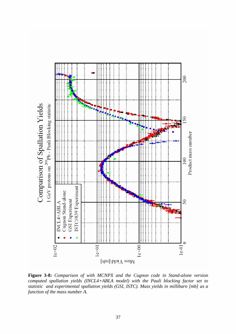
Figure 3-8: Comparison of with MCNPX and the Cugnon code in Stand-alone version computed spallation yields (INCL4+ABLA model) with the Pauli blocking factor set to statistic and experimental spallation yields (GSI, ISTC). Mass yields in millibarn [mb] as a function of the mass number A. ..................... 37
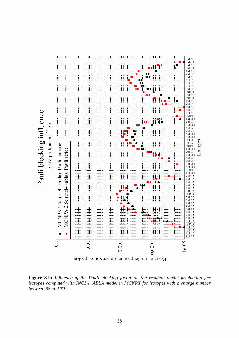
Figure 3-9: Influence of the Pauli blocking factor on the residual nuclei production per isotopes computed with INCL4+ABLA model in MCNPX for isotopes with a charge number between 68 and 70. ............................................................. 38
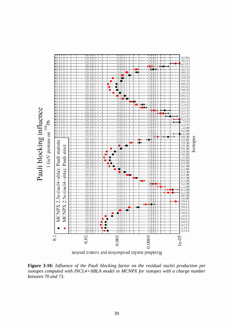
Figure 3-10: Influence of the Pauli blocking factor on the residual nuclei production per isotopes computed with INCL4+ABLA model in MCNPX for isotopes with a charge number between 70 and 73. ............................................................. 39
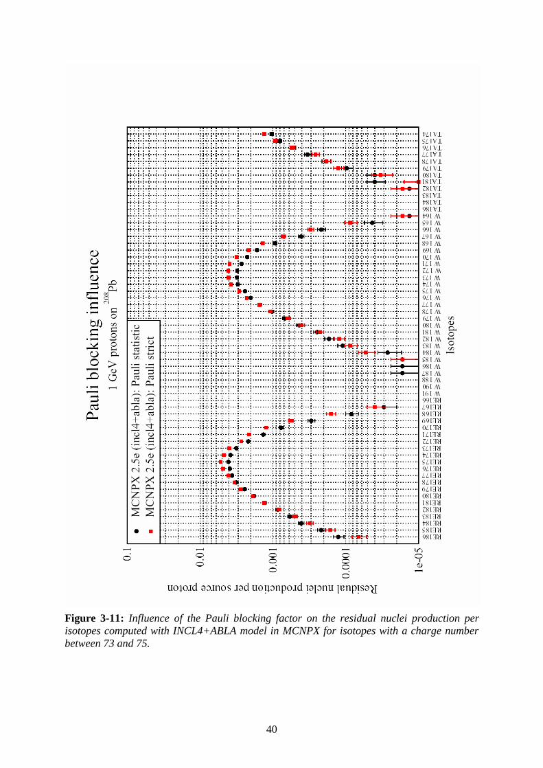
Figure 3-11: Influence of the Pauli blocking factor on the residual nuclei production per isotopes computed with INCL4+ABLA model in MCNPX for isotopes with a charge number between 73 and 75. ............................................................. 40
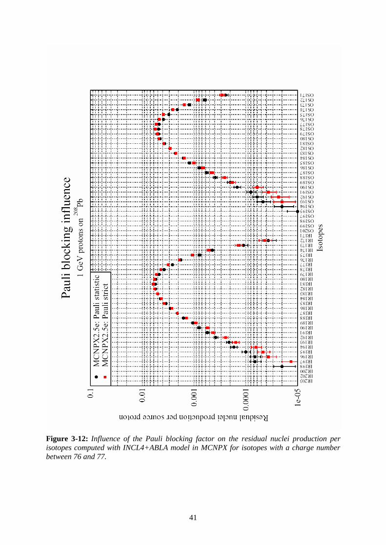
Figure 3-12: Influence of the Pauli blocking factor on the residual nuclei production per isotopes computed with INCL4+ABLA model in MCNPX for isotopes with a charge number between 76 and 77. ............................................................. 41
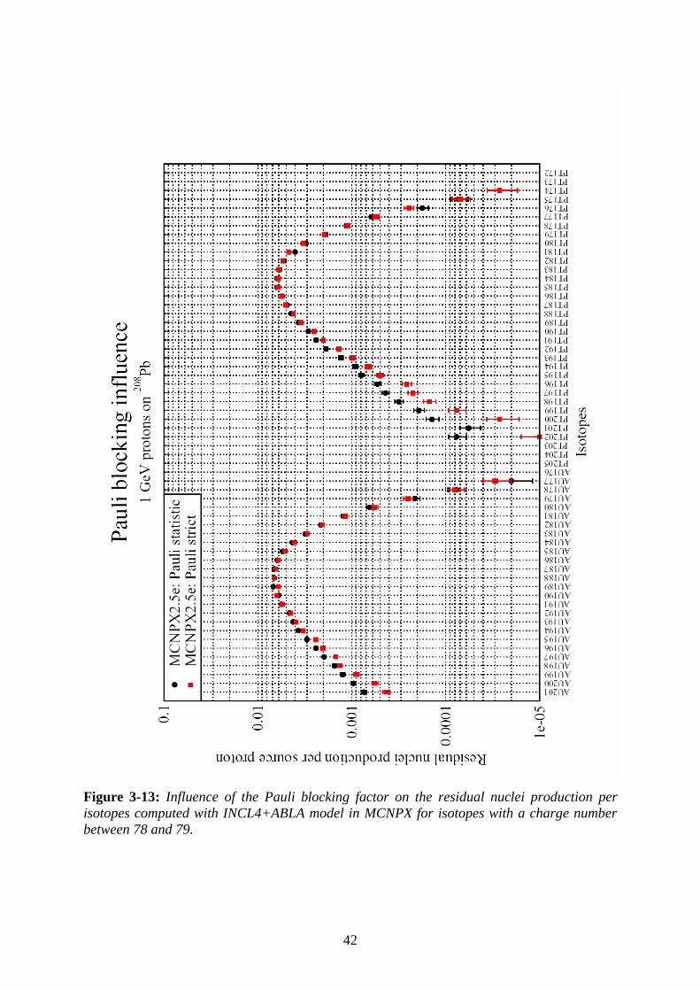
Figure 3-13: Influence of the Pauli blocking factor on the residual nuclei production per isotopes computed with INCL4+ABLA model in MCNPX for isotopes with a charge number between 78 and 79. ............................................................. 42
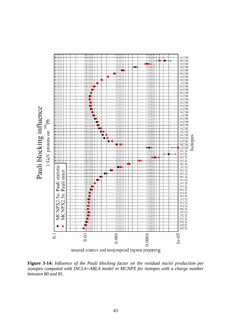
Figure 3-14: Influence of the Pauli blocking factor on the residual nuclei production per isotopes computed with INCL4+ABLA model in MCNPX for isotopes with a charge number between 80 and 81. ............................................................. 43
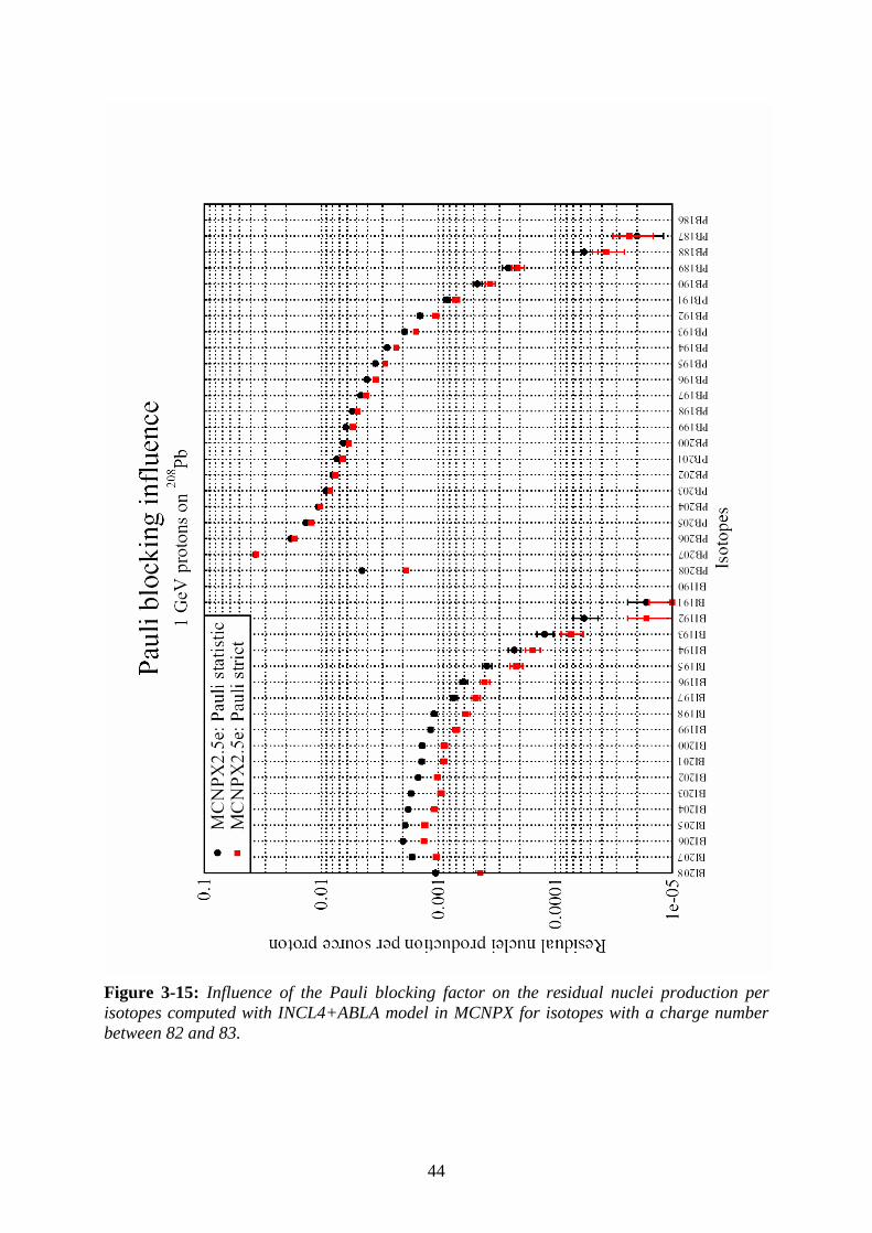
Figure 3-15: Influence of the Pauli blocking factor on the residual nuclei production per isotopes computed with INCL4+ABLA model in MCNPX for isotopes with a charge number between 82 and 83. ............................................................. 44
Figure 3-16: Comparison at 1 GeV proton energy on 208Pb of with MCNPX computed spallation yields (Bertini, ISABEL, INCL4+ABLA models) and experimental spallation yields (GSI [48], ISTC [46]). Mass yields in millibarn [mb] as a function of the mass number A. .................................................................... 47
Figure 3-17: Comparison at 600 MeV proton energy on 208Pb of with MCNPX and the Cugnon code in Stand-alone version computed spallation yields (INCL4+ABLA model) and experimental spallation yields (ISTC [49]). Mass yields in millibarn [mb] as a function of the mass number A. ..................... 49
Figure 3-18: Comparison at 600 MeV protons energy on 208Pb of with MCNPX and the Cugnon code in Stand-alone version computed spallation yields (INCL4+ABLA model) and experimental spallation yields (ISTC [49]). Charge yields in millibarn [mb] as a function of the charge number Z. ..... 50
vi
Figure 3-19: Comparison of with MCNPX (INCL4+ABLA model) (red triangle) and the Cugnon code in Stand-alone version (black square) computed spallation yields at 500 MeV protons energy and experimental spallation yields at 500 MeV (GSI [27, 50]). Mass yields in millibarn [mb] as a function of the mass number A. ..................................................................................................... 52
Figure 3-20: Comparison of with the Cugnon code in Stand-alone version computed spallation yields at 500 MeV protons energy with the Pauli blocking factor set to statistic (black square) and to strict (red triangle) and experimental spallation yields at 500 MeV (GSI [27, ,50]). Mass yields in millibarn [mb] as a function of the mass number A.................................................. 53
Figure 4-1: Test tube of the LiSoR experiment. ................................................................. 55 Figure 4-2: Schema of the LiSoR test tube and its cross section...................................... 56 Figure 4-3: MCNPX real geometry visualization of the LiSoR test tube cross section..... 56 Figure 4-4: LiSoR test tube cross section of the simplified geometry taken from [53]. .... 57 Figure 4-5: Comparison of the total activity of the Polonium isotopes directly after 34
hours irradiation. ......................................................................................... 67 Figure 4-6: Residual nuclei production in the LiSoR as a function of the mass number A.
...................................................................................................................... 68 Figure 4-7: Time dependence of the alpha-activity for the polonium isotopes. Alpha-
activity in Curies [Ci] as a function of the time. .......................................... 69 Figure 5-1: Sequence of the programs for the use of KAPROS for time dependence
calculations. ................................................................................................. 73 Figure 5-2: Flowchart of the different KAPROS programs related to the figure 5-1. ...... 74 Figure 5-3: Sequence of the programs to the use of ORIHET3 for time dependence
calculations. ................................................................................................. 77
vii
List of Tables Table 1-1: Main differences between the intranuclear cascades. ..................................... 11 Table 1-2: Main differences between the evaporation models.......................................... 13 Table 2-1: Cugnon Stand-alone input file and meaning of the different terms [32]......... 16 Table 3-1: Summary of the different combinations of LCA parameters and the
normalization associated.............................................................................. 24 Table 3-2: Reaction cross section for the Bertini code and for the Cugnon code. ........... 24 Table 3-3: Geometrical cross section from LAHET for the ISABEL model...................... 31 Table 3-4: Geometrical cross sections calculated with formulas from bibliography. ...... 31 Table 3-5: Input data for the calculation of the geometrical cross section for the Cugnon
model. .............................................................................................................. 32 Table 3-6: Geometrical cross section for 208Pb calculated by Cugnon according to the
formula (3.11)............................................................................................... 32 Table 3-7: Geometrical cross section for 208Pb calculated with the Sihver formula. ....... 32 Table 3-8: Summary of the geometrical cross section of the different models (Bertini,
ISABEL and INCL4 models) and of the parametrization from the bibliography. ................................................................................................ 33
Table 4-1: MCNPX input file for LiSoR calculations with the real geometry of the test tube. ................................................................................................................. 58
Table 4-2: Steel T91 composition in weight percentage, taken from [9].......................... 59 Table 4-3: Coolant composition in weight percentage, taken from [54]. ......................... 59 Table 4-4: Beam parameters for the LiSoR irradiation experiment. ................................ 60 Table 4-5: Alpha-activity of the Polonium isotopes after continuous irradiation at 50 μA.
......................................................................................................................... 63 Table 4-6: Production rates of Polonium isotopes just after irradiation and cooling time
of zero. ............................................................................................................. 64 Table 4-7: Alpha activities of Polonium isotopes just after irradiation and cooling time of
zero. ................................................................................................................. 64 Table 4-8: Branching ratio for the α-decays in percent used in references [53] and [54].
......................................................................................................................... 65 Table 4-9: Concentrations and alpha-activities of Polonium isotopes after continuous
irradiation. ................................................................................................... 66 Table 4-10: Total activity of the polonium isotopes for several simulations codes and for
the experiment. ............................................................................................. 67 Table 5-1: Input file for a KAPROS job. ........................................................................... 76 Table 5-2: Input file for an ORIHET3 job and meaning of somes terms. ......................... 78
1
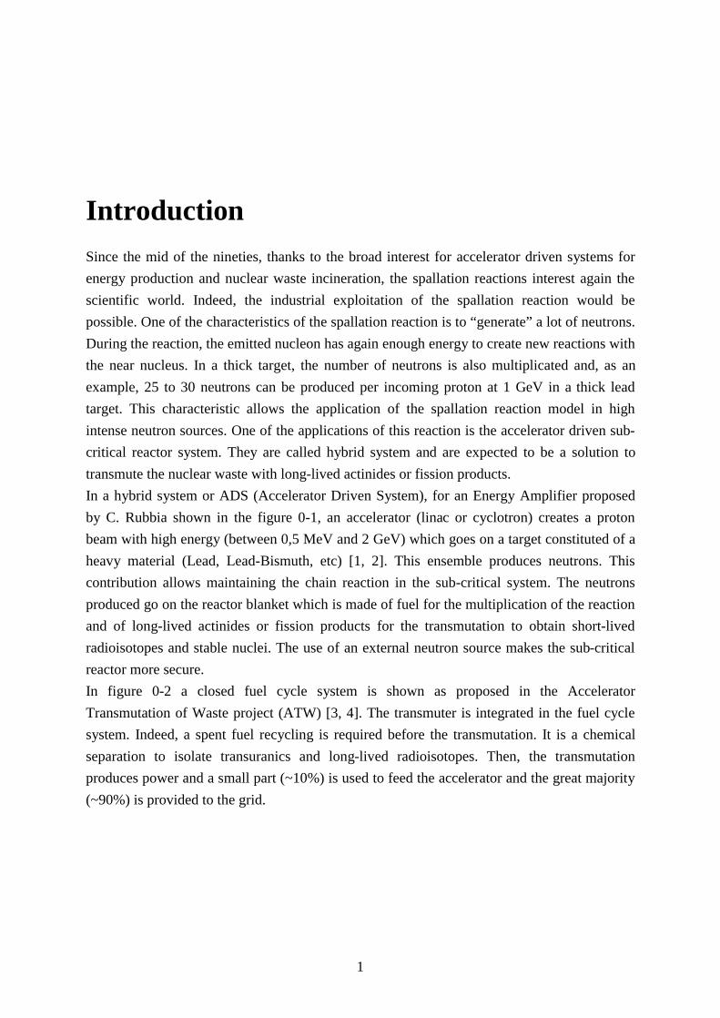
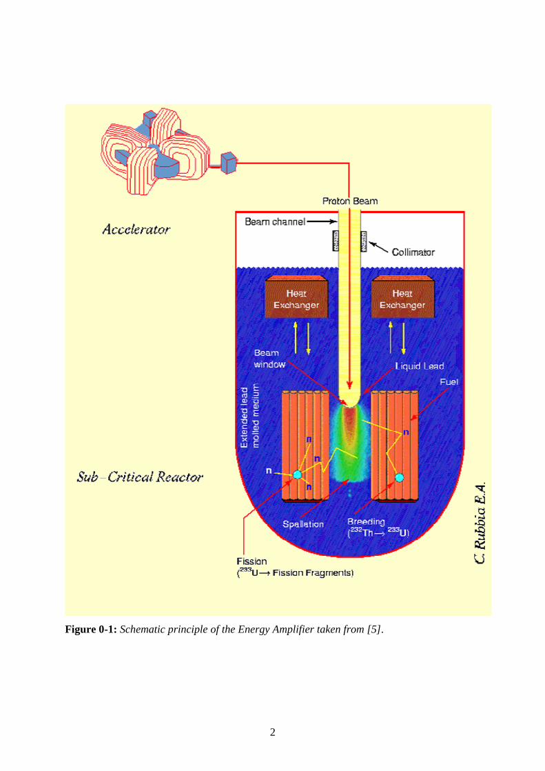
Introduction Since the mid of the nineties, thanks to the broad interest for accelerator driven systems for energy production and nuclear waste incineration, the spallation reactions interest again the scientific world. Indeed, the industrial exploitation of the spallation reaction would be possible. One of the characteristics of the spallation reaction is to “generate” a lot of neutrons. During the reaction, the emitted nucleon has again enough energy to create new reactions with the near nucleus. In a thick target, the number of neutrons is also multiplicated and, as an example, 25 to 30 neutrons can be produced per incoming proton at 1 GeV in a thick lead target. This characteristic allows the application of the spallation reaction model in high intense neutron sources. One of the applications of this reaction is the accelerator driven sub-critical reactor system. They are called hybrid system and are expected to be a solution to transmute the nuclear waste with long-lived actinides or fission products. In a hybrid system or ADS (Accelerator Driven System), for an Energy Amplifier proposed by C. Rubbia shown in the figure 0-1, an accelerator (linac or cyclotron) creates a proton beam with high energy (between 0,5 MeV and 2 GeV) which goes on a target constituted of a heavy material (Lead, Lead-Bismuth, etc) [1, 2]. This ensemble produces neutrons. This contribution allows maintaining the chain reaction in the sub-critical system. The neutrons produced go on the reactor blanket which is made of fuel for the multiplication of the reaction and of long-lived actinides or fission products for the transmutation to obtain short-lived radioisotopes and stable nuclei. The use of an external neutron source makes the sub-critical reactor more secure. In figure 0-2 a closed fuel cycle system is shown as proposed in the Accelerator Transmutation of Waste project (ATW) [3, 4]. The transmuter is integrated in the fuel cycle system. Indeed, a spent fuel recycling is required before the transmutation. It is a chemical separation to isolate transuranics and long-lived radioisotopes. Then, the transmutation produces power and a small part (~10%) is used to feed the accelerator and the great majority (~90%) is provided to the grid.
2
Figure 0-1: Schematic principle of the Energy Amplifier taken from [5].
3
Figure 0-2: Technical working groups of the ATW taken from [4]. This work will include various points: In chapter 1, we recall quickly the general basis of the spallation reaction as well as the various approaches used in the codes. We will study more particularly the physical models applied in the code INCL4 [6] for the intranuclear cascade and in the code ABLA [7, 8] for the evaporation model. The main programs and how they are connected in practice will be described in chapter 2. The main program for performing the simulation of the spallation reaction and the following transport calculations is MCNPX. The main objective of this study is the validation of the implementation of the codes of Cugnon and Schmidt in the new beta version 2.5e of MCNPX and it is developed in chapter 3. The spallation cross sections obtained for different proton energies compared to experimental data will be presented in chapter 3 too. Then, the chapter 4 is dedicated to the LiSoR experiment [9] which is a supporting experiment of the MEGAPIE project [1, 10]. Finally chapter 5 contains a comparison between two codes KAPROS [11] with the modul BURNUP[12] and ORIHET3 [13], which calculate the decay of isotopes. The physical basis of each program and the method to use them in practice is explained.
4
Chapter 1. Physicals Models E. O. Lawrence [14] had observed the spallation reaction for the first time in 1947. In 1952
the idea to use the spallation reaction as external source of a system of energy production is
developped. This sources of spallation neutron are important not only for the transmutation of
waste, but can be used for irradiation studies or material structure analyses and for tritium
production units [15].
This chapter will describe with more details the general features of the spallation reaction and its two stages. At the same time, we will give the charasteristics of a few modelisation codes which will be used in this work.
1.1. The spallation reaction
1.1.1. Mechanism and features The spallation reaction can be described as an interaction between a high energy light nucleus
(neutron, proton…) and a target heavy nucleus [16, 17]. The range of energy of the incoming
particles varies from a few hundreds of MeV to a few GeV per nucleon. At these energies, the
mechanism can be modeled following the idea of R. Serber [18]. He considers that the
reaction can be separated in two different steps: in the first, the wavelength associated with a
projectile of a few hundreds of MeV is about 10-14 cm. This length is smaller than the typical
inter-nucleonic distances in the target core (~ 1 fm=10-13 cm). The projectile sees also the
nucleons in the nucleus as individual particles and the reaction is a series of nucleon-nucleon
collisions. This stage is called intranuclear cascade. These successive collisions involve the
ejection of a few nucleons and the repartition of a part of the incoming energy on a big
number of nucleons and that leads to the excitation of the target nucleus which is yet called
pre-fragment. The second stage is the de-excitation of this pre-fragment via a process of
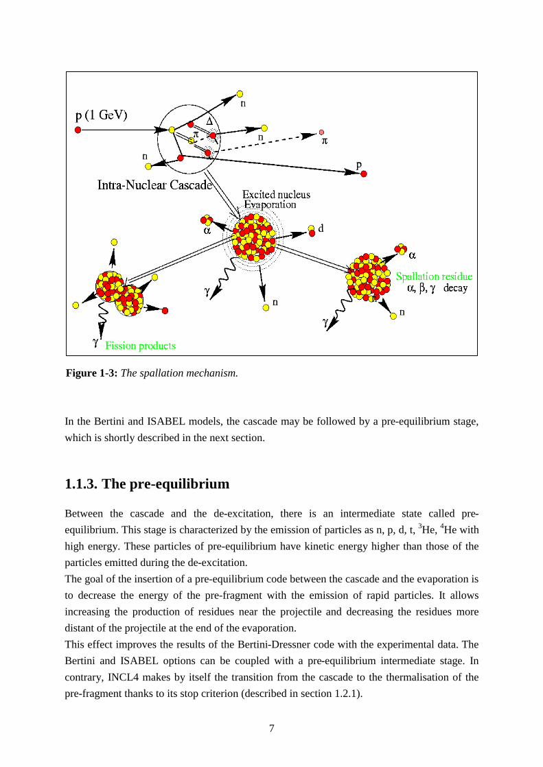
evaporation which may include the fission. If the particles (see figure 1-3) ejected during the
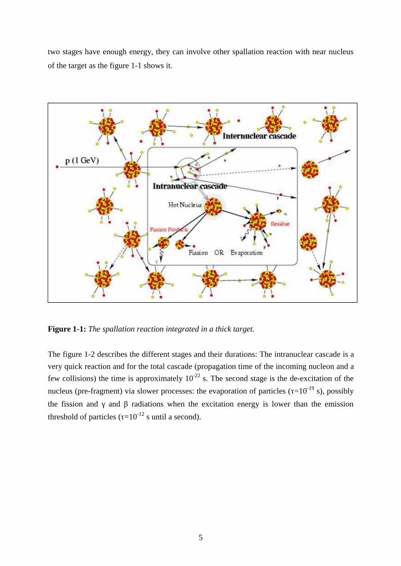
5
two stages have enough energy, they can involve other spallation reaction with near nucleus
of the target as the figure 1-1 shows it.
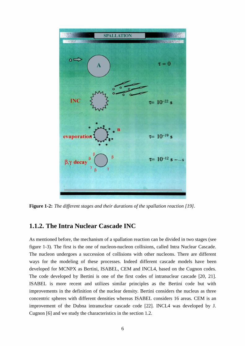
Figure 1-1: The spallation reaction integrated in a thick target. The figure 1-2 describes the different stages and their durations: The intranuclear cascade is a very quick reaction and for the total cascade (propagation time of the incoming nucleon and a few collisions) the time is approximately 10-22 s. The second stage is the de-excitation of the nucleus (pre-fragment) via slower processes: the evaporation of particles (τ=10-19 s), possibly the fission and γ and β radiations when the excitation energy is lower than the emission threshold of particles (τ=10-12 s until a second).
6
Figure 1-2: The different stages and their durations of the spallation reaction [19].
1.1.2. The Intra Nuclear Cascade INC As mentioned before, the mechanism of a spallation reaction can be divided in two stages (see figure 1-3). The first is the one of nucleon-nucleon collisions, called Intra Nuclear Cascade. The nucleon undergoes a succession of collisions with other nucleons. There are different ways for the modeling of these processes. Indeed different cascade models have been developed for MCNPX as Bertini, ISABEL, CEM and INCL4, based on the Cugnon codes. The code developed by Bertini is one of the first codes of intranuclear cascade [20, 21]. ISABEL is more recent and utilizes similar principles as the Bertini code but with improvements in the definition of the nuclear density. Bertini considers the nucleus as three concentric spheres with different densities whereas ISABEL considers 16 areas. CEM is an improvement of the Dubna intranuclear cascade code [22]. INCL4 was developed by J. Cugnon [6] and we study the characteristics in the section 1.2.
7
In the Bertini and ISABEL models, the cascade may be followed by a pre-equilibrium stage, which is shortly described in the next section.
1.1.3. The pre-equilibrium Between the cascade and the de-excitation, there is an intermediate state called pre-equilibrium. This stage is characterized by the emission of particles as n, p, d, t, 3He, 4He with high energy. These particles of pre-equilibrium have kinetic energy higher than those of the particles emitted during the de-excitation. The goal of the insertion of a pre-equilibrium code between the cascade and the evaporation is to decrease the energy of the pre-fragment with the emission of rapid particles. It allows increasing the production of residues near the projectile and decreasing the residues more distant of the projectile at the end of the evaporation. This effect improves the results of the Bertini-Dressner code with the experimental data. The Bertini and ISABEL options can be coupled with a pre-equilibrium intermediate stage. In contrary, INCL4 makes by itself the transition from the cascade to the thermalisation of the pre-fragment thanks to its stop criterion (described in section 1.2.1).
Figure 1-3: The spallation mechanism.
8
1.1.4. The de-excitation The first step of the spallation reaction produces an excited nucleus, called pre-fragment, which must decrease its energy level. Thus, the second step is the evaporation of light particles and/or fission. There exist 3 different ways for the de-excitation namely the multifragmentation, the fission and the evaporation. The probabilities of these possibilities depend on the nature of the nucleus and on the considered energy. The multifragmentation: With sufficient energy, near the energy of separation of the nucleus, mechanical instabilities break the nucleus in several fragments (more than two). The higher the energy is, the larger the number of fragments will be and their size will be small. This mode of de-excitation is principally present when there is a nucleus-nucleus collision. We will neglect this mode in our study proton on lead with 600-1000 MeV. The fission: Even in the case of a not very fissile nucleus, the available energy can lead to the fission of the nuclei in two fragments. We speak of “hot” fission for energy higher than 50 MeV. But, this phenomenon is remarkable only for nuclei of charge number higher than 75. The evaporation: The pre-fragment de-excites emitting principally nucleons, particles (d, t, 3He α) or light fragments (Isotopes of Lithium or Beryllium). The name evaporation comes from the similarity with the emission of molecules by a liquid in equilibrium with his gaseous form. We obtain also residual nucleus whose difference in mass compared to the pre-fragment depends directly on the energy deposited at the time of the first reaction. That is the mode we will observe in our study.
1.2. The Cugnon-Schmidt Model
1.2.1. The Cugnon cascade: INCL4 The Cugnon cascade is recent and relatively different of the earlier approach (Bertini, ISABEL and CEM models). The Cugnon cascade [6] was already described in references [15, 17, 23] and the main characteristics are recalled in this section. All the features of the INCL4 cascade are discussed in [24].
9
The medium The type of medium is the main criterion to differentiate the different codes. The Bertini and ISABEL codes were based on a nuclear model in which the nucleon density within the nucleus was supposed constant within certain areas (see section 1.1.2) and where the nucleons are not considered individually except the cascade particles. The INCL4 code doesn’t consider the nucleus as a continuous medium but as a bundle of individual nucleons moving in a given potential. The criterion of collision To determinate the moment where the interaction proton-nucleon has to take place two approaches are often used. In the beginning, the particles are propagating freely until the
distance between two of them is lower than a preset minimal distance minijd (INCL4 code).
π
σ )(min ijijij
sd = (1.1)
where )( ijij sσ is the total interaction cross section at the available energy ijs in the centre of
mass system. A radically different approach considers the nucleus as a continuous medium in which the particles have a mean free path. After this path, they collide with a nucleon which takes itself a free course and so on (Bertini and ISABEL codes). The time interval is given by the minimal value of:
⟩⟨=∆
i
i
nβλ
τ min (1.2)
where ⟩⟨ iλ is the mean free path of each cascade particles, iβ is their velocity and n is a
parameter fixed to 20=n . The stopping time The cascade is considered as finished when the nucleus reached a balanced thermal state. Here too, two approaches exist. One is based on time: the equilibrium state is supposed to be reached with the end of one given time (INCL4 code). The new version integrates a dependence of the stopping time with the target nucleus given by:
( ) 16.0
2080TA
stopstop tft = (1.3)
10
where stopf is an adjustable parameter and the default value is equal to 1, cfmt /700 = , and
TA is the atom mass of the target nucleus.
The other is based on the energy: the cascade is considered finished when all the nucleons have an energy lower than a definite threshold called cut-off energy cutE (Bertini and
ISABEL codes). The nuclear surface The treatment of the nuclear surface parameter is an important feature of the INCL4 code. In the earlier options of MCNPX (Bertini, ISABEL codes) the collisions of the nucleons take place in a mean field described by a potential well with an abrupt surface:
31
2.1 AR = (1.4) In the INCL4 code the density is given by a Wood-Saxon function:
(1.5)
Where
( ) fmAAR TT3
140 063.110.745.2 += − (1.6)
fmAa T
410.63.1510.0 −+= (1.7)
aRR 80max += (1.8) The Pauli blocking The Pauli principle means that there cannot be, in an atomic nucleus, two nucleons which have the same characterizing features. These characteristics are the type of nucleon (neutron or proton), the energy state, the angular momentum (spin) and the z-component of the spin. In the Fermi gas model for the atomic nucleus, which is put in the computations for the intranuclear cascade, all possible nucleon states are occupied. The Fermi energy is the highest energy, which a nucleon can have in the nucleus in this Fermi gas model [25]. If during the intranuclear cascade a nucleon comes out, whose energy is smaller than the Fermi energy, and if there is already a nucleon in the nucleus with the same quantum numbers, thus the state is already occupied. With the “strict” application of the Pauli principle therefore later all processes are excluded, in which a nucleon occurs with an energy, which is smaller than Fermi energy. However too many processes are excluded. In the course of the intranuclear
)exp(1 0
0
aRr −+
ρ
0
=ρ
maxRrfor >
maxRrfor <
11
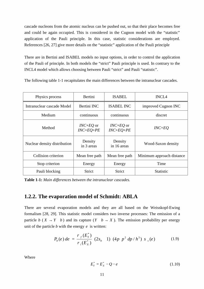
cascade nucleons from the atomic nucleus can be pushed out, so that their place becomes free and could be again occupied. This is considered in the Cugnon model with the “statistic” application of the Pauli principle. In this case, statistic considerations are employed. References [26, 27] give more details on the “statistic” application of the Pauli principle There are in Bertini and ISABEL models no input options, in order to control the application of the Pauli of principle. In both models the “strict” Pauli principle is used. In contrary to the INCL4 model which allows choosing between Pauli “strict” and Pauli “statistic”. The following table 1-1 recapitulates the main differences between the intranuclear cascades.
Physics process Bertini ISABEL INCL4
Intranuclear cascade Model Bertini INC ISABEL INC improved Cugnon INC
Medium continuous continuous discret
Method INC+EQ or INC+EQ+PE
INC+EQ or INC+EQ+PE INC+EQ
Nuclear density distribution Density in 3 areas
Density in 16 areas Wood-Saxon density
Collision criterion Mean free path Mean free path Minimum approach distance
Stop criterion Energy Energy Time
Pauli blocking Strict Strict Statistic
Table 1-1: Main differences between the intranuclear cascades.
1.2.2. The evaporation model of Schmidt: ABLA There are several evaporation models and they are all based on the Weisskopf-Ewing formalism [28, 29]. This statistic model considers two inverse processes: The emission of a particle b ( bYX +→ ) and its capture ( XbY →+ ). The emission probability per energy unit of the particle b with the energy ε is written: (1.9) Where
ε−−= QEE XY** (1.10)
)( ) / (4 1) 2( )()(
)( c32
*
*
εσπρ
ρεε ⋅⋅+⋅= hdpps
EE
dP bXi
Yfb
12
Where
bs : Spin of particle b
iρ : The level density of the nucleus X
fρ : The level density of the nucleus Y
Q : The difference of mass excess 32 /4 hdppπ : The number of states with a momentum between p and dpp +
( )εσ c : The capture cross section for the particle b by the nucleus Y *YE : The energy of the nucleus Y *XE : The energy of the nucleus X
The emission probability depends on state density ρ and capture cross-section cσ .
The code ABLA was developed at the GSI at the beginning of the eighties by K.H Schmidt and his collaborators [7, 8] and reference [26] presents the basis. In this code, the particles which can be evaporated are only n, p, and alpha particles in contrary to the Dresner code which allows the evaporation of p, n, d, 3H, 3He, 4He. The most recent parameterizations of the density level and of the parameter of the density levels are in the article of Junghans et al. [30].
4/54/1
2/1
´12)(
EaeE
Sπρ = (1.11)
with
( ) ( )( )[ ] 2/1´.´.´2 EhPEfUEaS δδ ++= (1.12)
The functions ( ) EEf / and ( ) EEh / tend toward 0 at high energy and toward 1 at low energy.
´Uδ accounts for the shell effect and ´Pδ for the pairing. The parameter ´a is another parameterization by Ignatyuk:
KksSv BABAAa 3/13/2´ ααα ++= (1.13)
with 1073.0 −= MeVvα the volume coefficient, 1095.0 −= MeVSα the surface coefficient
and 10 −= MeVkα the coefficient of bending. BS represents the surface of the nucleus
13
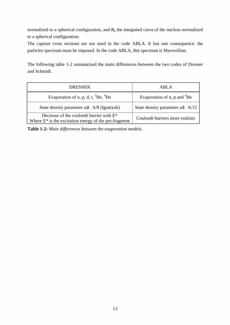
normalized to a spherical configuration, and Bk the integrated curve of the nucleus normalized to a spherical configuration. The capture cross sections are not used in the code ABLA. It has one consequence: the particles spectrum must be imposed. In the code ABLA, this spectrum is Maxwellian. The following table 1-2 summarized the main differences between the two codes of Dresner and Schmidt.
DRESNER ABLA
Evaporation of n, p, d, t, 3He, 4He Evaporation of n, p and 4He
State density parameter aà A/8 (Ignatyuk) State density parameter aà A/12
Decrease of the coulomb barrier with E* Where E* is the excitation energy of the pre-fragment Coulomb barriers more realistic
Table 1-2: Main differences between the evaporation models.
14
Chapter 2. Simulation codes To study this complex reaction, it is necessary to use simulations which describe the spallation reaction and the transport of particles in a thick target. In a thick target the interaction between a particle and the material is very complex because several reactions at different energy levels can take place. The simulation of the mechanism of the spallation reaction is very complicated and no analytic solution could be found. That’s why the statistic treatment with the Monte Carlo method is the applied option. All the existing codes are based on this Monte Carlo method. The Monte Carlo methods consist of experimental or data-processing simulations of mathematical or physical problems, based on the pulling of random numbers. Generally one uses in fact a series of pseudo-random numbers generated by specialized algorithms. The properties of these series are very close to those of a true random walk. To obtain statistically reliable results, it is necessary to evaluate a lot of histories.
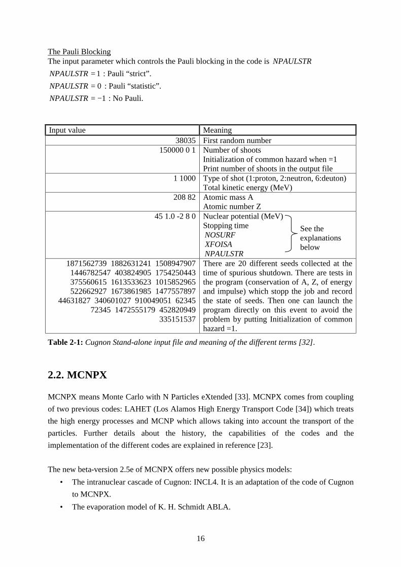
2.1. The Cugnon code in the Stand-alone version This program has been developed by J. Cugnon at the University of Liege. He uses his model of the intra nuclear cascade. The input file for Cugnon Stand-alone code, shown in table 2-1 allows running a job. The main input parameters are the nuclear potential, stopf which
controls the stopping time, NOSURF which controls the nuclear surface, XFOISA which controlls the parameter of maximum impact and the Pauli blocking. Their meanings are described below. The nuclear potential The nuclear potential or potential depth is coded in the Cugnon code in Stand-alone version by V0 and the default value is fixed to 45 MeV. It is the value generally used for heavy nucleus. Reference [31] gives a parameterization of the potential depth in the valley of stability as a function of the mass number. The equation system (2.1) shows this
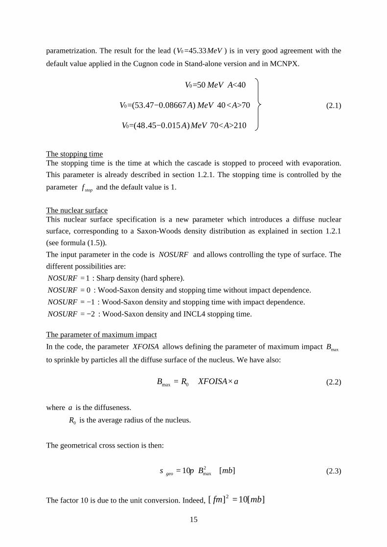
15
parametrization. The result for the lead ( MeVV 33.450 = ) is in very good agreement with the
default value applied in the Cugnon code in Stand-alone version and in MCNPX. 40500 <= AMeVV
7040)08667.047.53(0 ><−= AMeVAV (2.1) 21070)015.045.48(0 ><−= AMeVAV The stopping time The stopping time is the time at which the cascade is stopped to proceed with evaporation. This parameter is already described in section 1.2.1. The stopping time is controlled by the parameter stopf and the default value is 1.
The nuclear surface This nuclear surface specification is a new parameter which introduces a diffuse nuclear surface, corresponding to a Saxon-Woods density distribution as explained in section 1.2.1 (see formula (1.5)). The input parameter in the code is NOSURF and allows controlling the type of surface. The different possibilities are:
1=NOSURF : Sharp density (hard sphere). 0=NOSURF : Wood-Saxon density and stopping time without impact dependence.
1−=NOSURF : Wood-Saxon density and stopping time with impact dependence. 2−=NOSURF : Wood-Saxon density and INCL4 stopping time.
The parameter of maximum impact In the code, the parameter XFOISA allows defining the parameter of maximum impact maxB
to sprinkle by particles all the diffuse surface of the nucleus. We have also:
aXFOISARB ×+= 0max (2.2)
where a is the diffuseness. 0R is the average radius of the nucleus.
The geometrical cross section is then:
][10 2max mbBgeo πσ = (2.3)
The factor 10 is due to the unit conversion. Indeed, ][10][ 2 mbfm =
16
The Pauli Blocking The input parameter which controls the Pauli blocking in the code is NPAULSTR
1=NPAULSTR : Pauli “strict”. 0=NPAULSTR : Pauli “statistic”.
1−=NPAULSTR : No Pauli. Input value Meaning
38035 First random number 150000 0 1 Number of shoots
Initialization of common hazard when =1 Print number of shoots in the output file
1 1000 Type of shot (1:proton, 2:neutron, 6:deuton) Total kinetic energy (MeV)
208 82 Atomic mass A Atomic number Z
45 1.0 -2 8 0 Nuclear potential (MeV) Stopping time NOSURF XFOISA NPAULSTR
1871562739 1882631241 1508947907 1446782547 403824905 1754250443 375560615 1613533623 1015852965 522662927 1673861985 1477557897
44631827 340601027 910049051 62345 72345 1472555179 452820949
335151537
There are 20 different seeds collected at the time of spurious shutdown. There are tests in the program (conservation of A, Z, of energy and impulse) which stopp the job and record the state of seeds. Then one can launch the program directly on this event to avoid the problem by putting Initialization of common hazard =1.
Table 2-1: Cugnon Stand-alone input file and meaning of the different terms [32].
2.2. MCNPX MCNPX means Monte Carlo with N Particles eXtended [33]. MCNPX comes from coupling of two previous codes: LAHET (Los Alamos High Energy Transport Code [34]) which treats the high energy processes and MCNP which allows taking into account the transport of the particles. Further details about the history, the capabilities of the codes and the implementation of the different codes are explained in reference [23]. The new beta-version 2.5e of MCNPX offers new possible physics models:
• The intranuclear cascade of Cugnon: INCL4. It is an adaptation of the code of Cugnon to MCNPX.
• The evaporation model of K. H. Schmidt ABLA.
See the explanations below
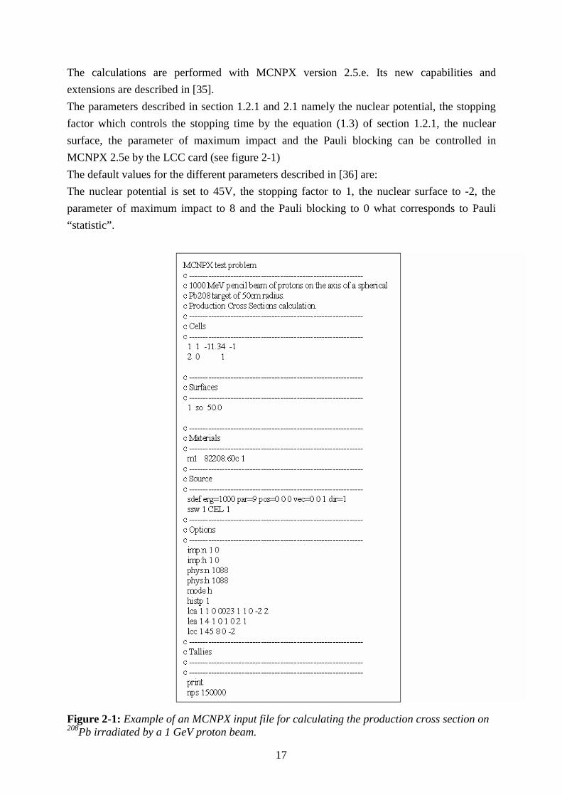
17
The calculations are performed with MCNPX version 2.5.e. Its new capabilities and extensions are described in [35]. The parameters described in section 1.2.1 and 2.1 namely the nuclear potential, the stopping factor which controls the stopping time by the equation (1.3) of section 1.2.1, the nuclear surface, the parameter of maximum impact and the Pauli blocking can be controlled in MCNPX 2.5e by the LCC card (see figure 2-1) The default values for the different parameters described in [36] are: The nuclear potential is set to 45V, the stopping factor to 1, the nuclear surface to -2, the parameter of maximum impact to 8 and the Pauli blocking to 0 what corresponds to Pauli “statistic”.
Figure 2-1: Example of an MCNPX input file for calculating the production cross section on 208Pb irradiated by a 1 GeV proton beam.
18
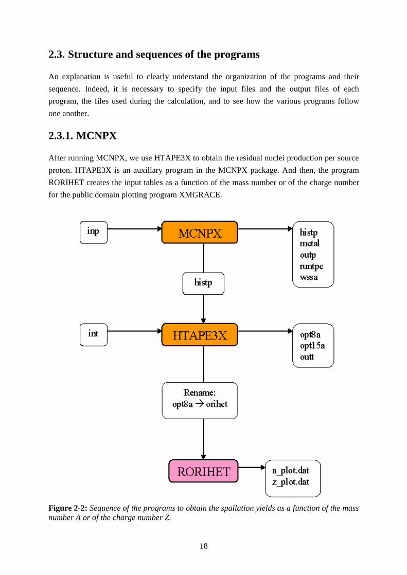
2.3. Structure and sequences of the programs An explanation is useful to clearly understand the organization of the programs and their sequence. Indeed, it is necessary to specify the input files and the output files of each program, the files used during the calculation, and to see how the various programs follow one another.
2.3.1. MCNPX After running MCNPX, we use HTAPE3X to obtain the residual nuclei production per source proton. HTAPE3X is an auxillary program in the MCNPX package. And then, the program RORIHET creates the input tables as a function of the mass number or of the charge number for the public domain plotting program XMGRACE.
Figure 2-2: Sequence of the programs to obtain the spallation yields as a function of the mass number A or of the charge number Z.
19
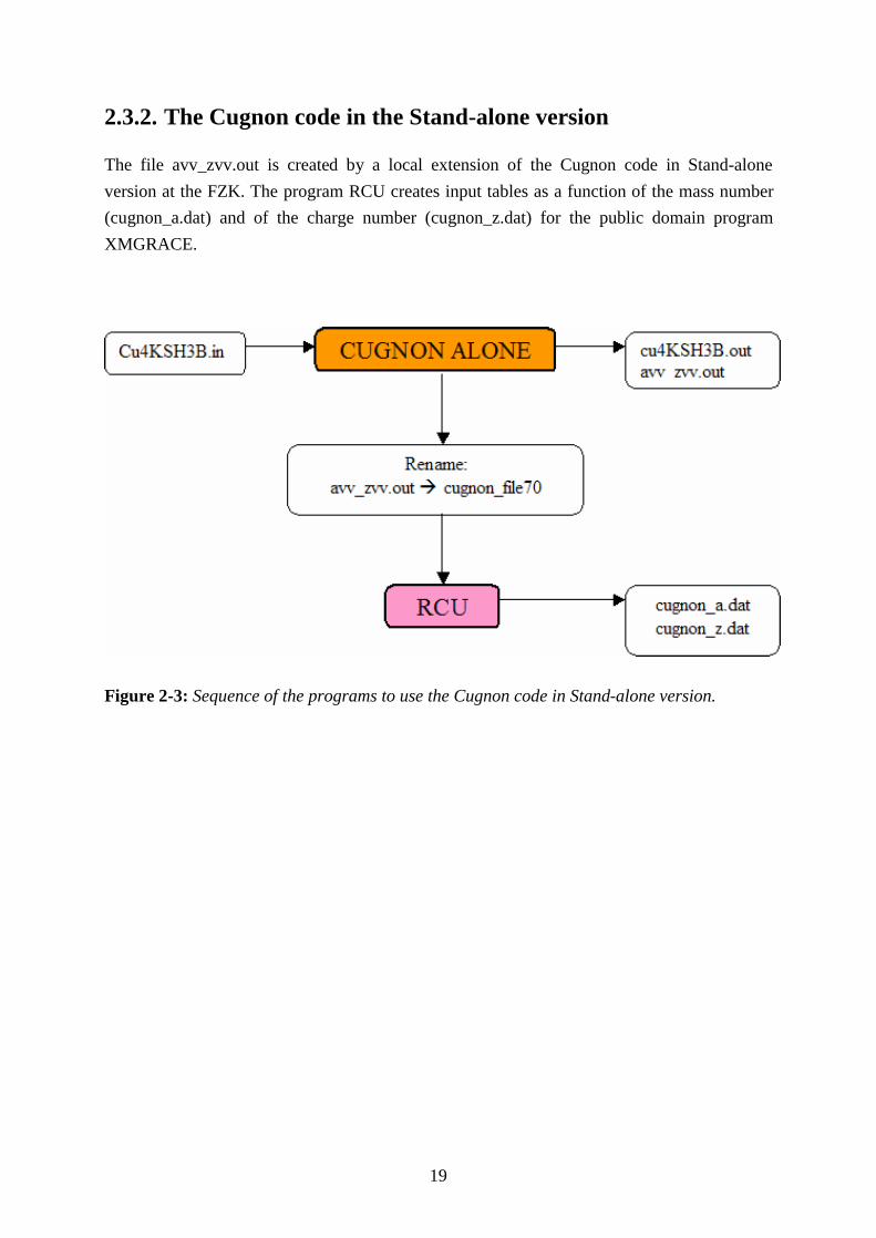
2.3.2. The Cugnon code in the Stand-alone version The file avv_zvv.out is created by a local extension of the Cugnon code in Stand-alone version at the FZK. The program RCU creates input tables as a function of the mass number (cugnon_a.dat) and of the charge number (cugnon_z.dat) for the public domain program XMGRACE.
Figure 2-3: Sequence of the programs to use the Cugnon code in Stand-alone version.
20
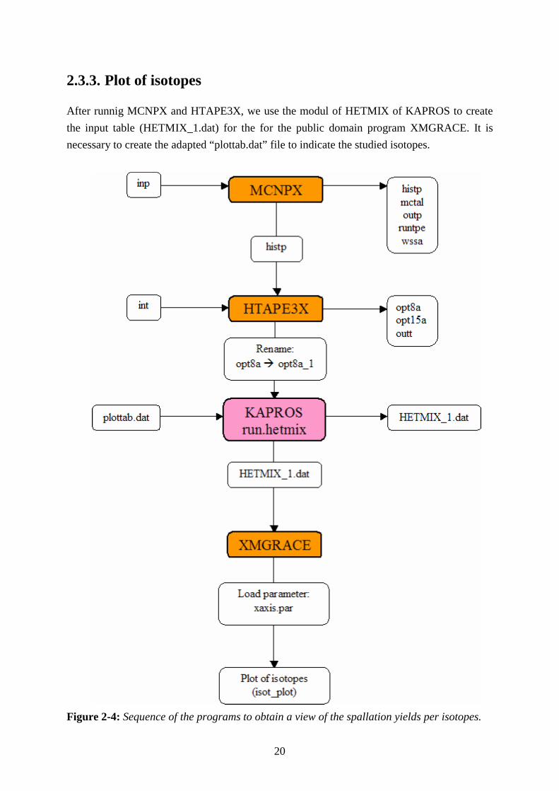
2.3.3. Plot of isotopes After runnig MCNPX and HTAPE3X, we use the modul of HETMIX of KAPROS to create the input table (HETMIX_1.dat) for the for the public domain program XMGRACE. It is necessary to create the adapted “plottab.dat” file to indicate the studied isotopes.
Figure 2-4: Sequence of the programs to obtain a view of the spallation yields per isotopes.
21
Chapter 3. Comparison of MCNPX with the INCL4-
ABLA model and the Cugnon-Schmidt code
in the Stand-alone version The purpose of this part is the comparison of the Cugnon-Schmidt in Stand-alone program and INCL4-ABLA implementation in MCNPX.
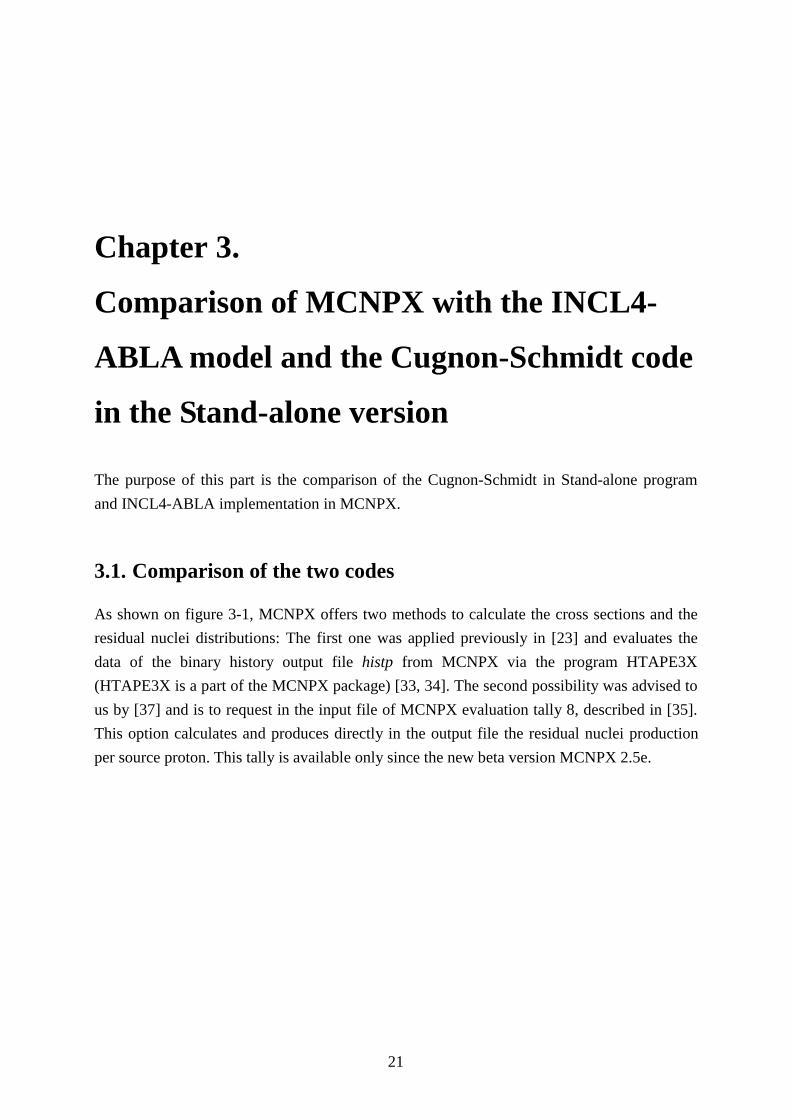
3.1. Comparison of the two codes As shown on figure 3-1, MCNPX offers two methods to calculate the cross sections and the residual nuclei distributions: The first one was applied previously in [23] and evaluates the data of the binary history output file histp from MCNPX via the program HTAPE3X (HTAPE3X is a part of the MCNPX package) [33, 34]. The second possibility was advised to us by [37] and is to request in the input file of MCNPX evaluation tally 8, described in [35]. This option calculates and produces directly in the output file the residual nuclei production per source proton. This tally is available only since the new beta version MCNPX 2.5e.
22
Figure 3-1: Two different methods of treatments to obtain the spallation yields in MCNPX. We have checked that the two methods give exactly the same distribution before normalization. The output files of HTAPE3X and of the direct computation with tally 8 option can be consulted in annex A. These calculations were obtained by irradiation of a 208Pb target at 1 GeV protons beam and by running 300.000 particles. To obtain the spallation yields, it is necessary to normalize the distributions. We have analyzed how the normalization factor must be determined according to the type of reactions which one studies. When a proton collides with a target nucleus in a non-elastic reaction, this collision can give rise to a cascade (spallation reaction) but, in other cases, the incoming proton can pass through the target nuclei without any interaction (transparency). The input parameters allow us to choose between a forced cascade or cascade with transparencies. There are four input cards (LCA, LCB, LEA and LEB) in MCNPX [33] which allow the user controlling the physics options. We will be interested more particularly in the LCA card. The LCA card is used to select the Bertini, ISABEL, CEM or INCL4 models, as well as to set certain parameter used in these models which are discussed thereafter. We want to obtain the cross sections. It means that only the first interaction of the source particle is taken into account. Thus, the transport and the slowing-down are turned off. This option is controlled by the eighth parameter of the LCA card, called NOACT. There are two values of this parameter which allow obtaining the cross sections. It is -1 and -2. NOACT equal to -1 is used to compute with HTAPE3X code. The NOACT equal to -2 is used to compute double-differential cross sections and residual nuclei with the tally 8 option. If a cascade is forced, we must use the reaction cross section to normalize the yields.
23
One can use as a normalization factor, either
particles
reaction
Nσ
(3.1)
Or
ciestransparenparticles
geo
NN −
σ (3.2)
with 2Rgeo πσ = (3.3).
In section 3.2 the geometrical cross section geoσ is investigated in more detail.
In the Cugnon code in the stand-alone version, the reaction is not forced (there are transparencies) and thus, the use of geometrical cross section for the normalization is correct. In contrary, in MCNPX, to obtain cross sections, we must set the NOACT parameter to -1 or -2 which corresponds to a forced cascade. So, it is not possible to normalize with the geometrical cross section. The value of the reaction cross section coming from the Bertini model is 1732 mb. This value is obtained from the LAHET output file which gives the number of transparencies and the geometrical cross section. Then:
geoparticles
ciestransparenparticlesreaction N
NNσσ
−= (3.4)
The INCL4 model gives a cross section reaction value equal to 1793 mb. The difference is approximately of 3%. Thus we can conclude that the reaction cross section is not very different according to the model. In the calculations the reaction cross section is fixed in an early stage to 1740 mb. A second input parameter for MCNPX is relevant for this question. It is the first parameter of the LCA card, called IELAS. It controls if the elastic scattering for neutrons and protons are taken into account. The program XSEX3 which is a part of the MCNPX package [33] could provide the number of elastic scattering but the conditions to obtain this value are not yet completely clear, so we can not present results normalized with this method. But in the case where the number of elastic scattering is given we can normalize the yields. Indeed, it is necessary to subtract them to the number of events.
24
So, to summarize: • If a cascade is forced, we must normalize with the reaction cross section. • If a cascade is not forced (there are transparencies), we can normalize with the
geometrical cross section. • If the elastic scattering reactions are taken into account, we need their number and
then we can normalize.
The calculations with NOACT equal to -2 give a number of nonzero history tallies different of the number of particles and it must be taken into account in the normalization. As a conclusion we recommend to use no elastic scattering for protons (IELAS=0 or 1) and to force the reactions with the NOACT parameter recommended for the tally 8 option (NOACT=-2). For an example, that corresponds to the following LCA card with the INCL4 model: lca 1 0 0 0023 1 1 0 -2 2. The normalization factor corresponding to this card is
reactionσnsinteractionuclear ofNumber
particles ofNumber (3.5)
IELAS NOACT Normalization 1 -1 Reaction cross section 1 -2 Reaction cross section 2 -1 Geometrical cross section 2 -2 Geometrical cross section
Table 3-1: Summary of the different combinations of LCA parameters and the normalization associated.
Model Bertini Cugnon Reaction cross section [mb] 1732 1793
Table 3-2: Reaction cross section for the Bertini code and for the Cugnon code. Perspectives:
• An interesting extension would be to obtain in a reliable way the number of elastic scattering and to check the normalization.
• Then, more precise determination of the reaction cross section for the different physical models is necessary.
• Signification of using the number of nuclear nonzero history tallies different of the events.
25
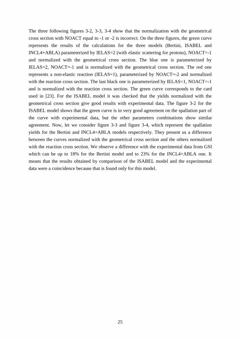
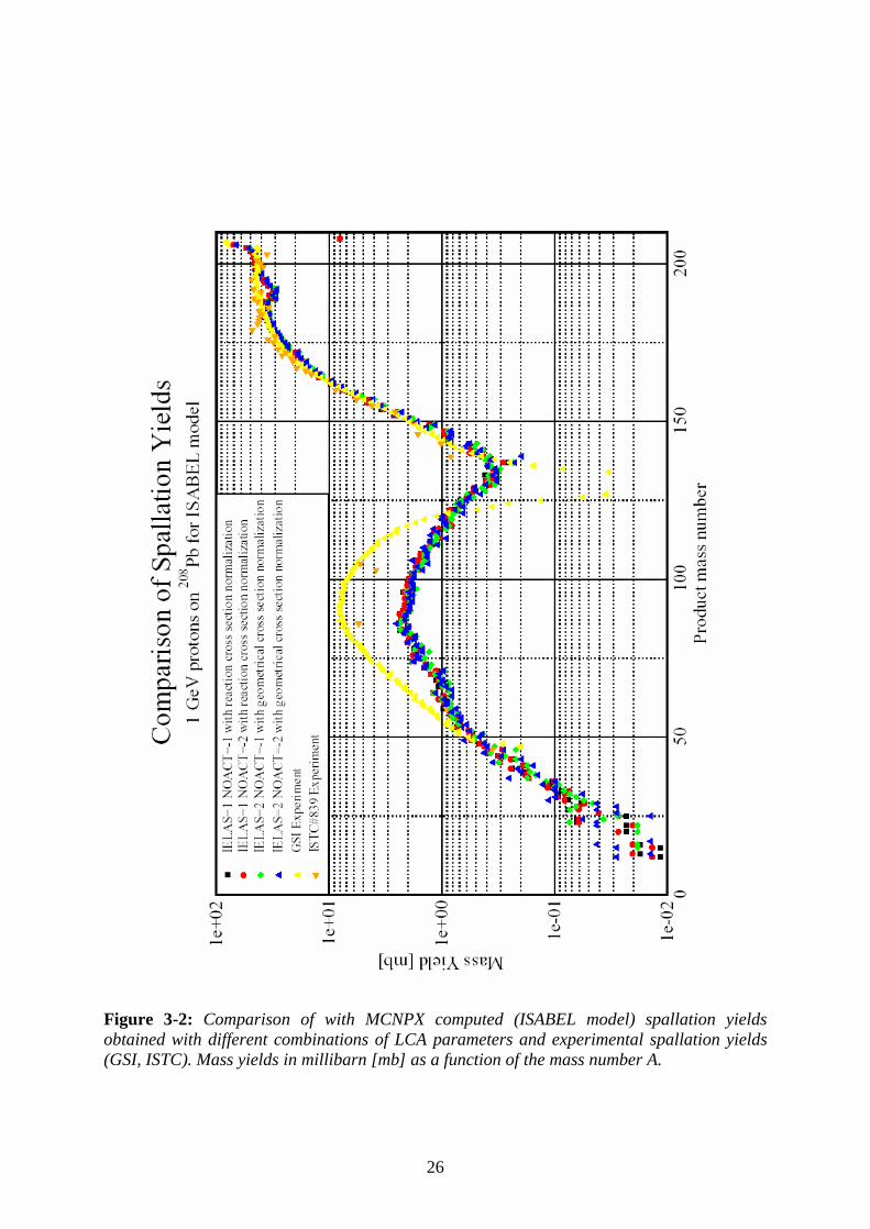
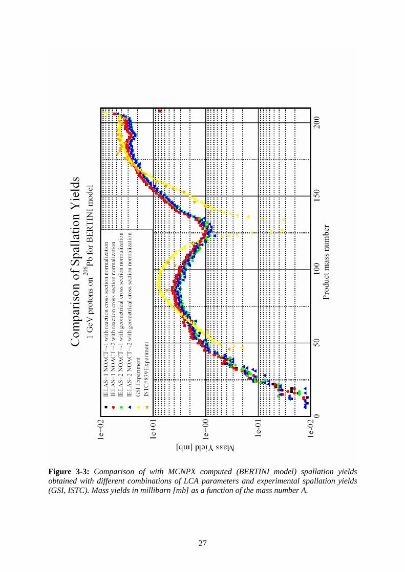
The three following figures 3-2, 3-3, 3-4 show that the normalization with the geometrical cross section with NOACT equal to -1 or -2 is incorrect. On the three figures, the green curve represents the results of the calculations for the three models (Bertini, ISABEL and INCL4+ABLA) parameterized by IELAS=2 (with elastic scattering for protons), NOACT=-1 and normalized with the geometrical cross section. The blue one is parameterized by IELAS=2, NOACT=-1 and is normalized with the geometrical cross section. The red one represents a non-elastic reaction (IELAS=1), parameterized by NOACT=-2 and normalized with the reaction cross section. The last black one is parameterized by IELAS=1, NOACT=-1 and is normalized with the reaction cross section. The green curve corresponds to the card used in [23]. For the ISABEL model it was checked that the yields normalized with the geometrical cross section give good results with experimental data. The figure 3-2 for the ISABEL model shows that the green curve is in very good agreement on the spallation part of the curve with experimental data, but the other parameters combinations show similar agreement. Now, let we consider figure 3-3 and figure 3-4, which represent the spallation yields for the Bertini and INCL4+ABLA models respectively. They present us a difference between the curves normalized with the geometrical cross section and the others normalized with the reaction cross section. We observe a difference with the experimental data from GSI which can be up to 18% for the Bertini model and to 23% for the INCL4+ABLA one. It means that the results obtained by comparison of the ISABEL model and the experimental data were a coincidence because that is found only for this model.
26
Figure 3-2: Comparison of with MCNPX computed (ISABEL model) spallation yields obtained with different combinations of LCA parameters and experimental spallation yields (GSI, ISTC). Mass yields in millibarn [mb] as a function of the mass number A.
27
Figure 3-3: Comparison of with MCNPX computed (BERTINI model) spallation yields obtained with different combinations of LCA parameters and experimental spallation yields (GSI, ISTC). Mass yields in millibarn [mb] as a function of the mass number A.
28
Figure 3-4: Comparison of with MCNPX computed (INCL4+ABLA model) spallation yields obtained with different combinations of LCA parameters and experimental spallation yields (GSI, ISTC). Mass yields in millibarn [mb] as a function of the mass number A.
29
3.2. Investigations related to the normalization factor To compare the data given by the output file opt8a from the HTAPE3X program of the MCNPX package with experimental data, we need the normalization factor. The purpose of this part is the analysis of the normalization factor for spallation yields. In order to get confidence in the results of simulation codes, validation by comparison with experimental data is necessary. The qualification of the simulation of the reaction products produced by irradiation of a target by high energetic protons is still in progress. Two types of experiments are applied for this purpose: thin or thick targets. In the thin target experiments, only primary reactions are measured, whereas in thick target reaction cascades are investigated. Both types of investigation are discussed in reference [23]. In this section, the validation is analyzed in more detail. The considered target experiments are carried out by direct proton irradiation (ISTC) or by the inverse kinematic method (GSI). The results of these experiments are cross sections for spallation products. As the simulation code MCNPX and its evaluation program HTAPE3X calculates spallation products yields per source proton, a normalization factor is required for the comparison. This normalization factor is discussed in section 3.2.1 and it is show that the geometrical cross section geoσ plays an important role.
3.2.1. Formulations for the nucleus geometry The formulation and the description of the geometry of the nucleus influence the distribution of the spallation yields. Now we analyze several formulations for the geometry of nucleus.
3.2.1.1. Range of the nucleus radius The geometrical cross section is given by the following formula:
(3.6)
where R is the radius of the nuclei. Thus, to obtain the geometrical cross section, it is necessary to determine the radius R of the nuclei. It is considered, as a first approximation, that the nucleus has a spherical form and that it has an incompressible volume.The volume of the hydrogen nuclei is noted 0V :
(3.7)
2Rgeo πσ =
30 3
4 RV π=
30
If one considers that the volume of the atomic nucleus is proportional to the number of nucleons which constitute the nucleus:
(3.8)
The radius of a nucleus is proportional to the cubic root of the number of particles. One deduces:
(3.9) where fmr 2.10 = from [38] fmr 43.10 = from [39]
The exact value of 0r is somewhat contentious, and different types of experiment give values
of 0r ranging from 1.07 to 1.6 [39]. As an example, Bethe has found cmr 130 10.47.1 −= [40],
and Barkas cmr 130 10.43.1 −= [41]. The geometrical cross sections obtained with this
different value 0r are summarized in the table 3-4. We can observe that the best result in
comparison with the Cugnon and ISABEL values is obtained with fmr 6.10 = .
From other experiments, nuclear radius can be found from measurements of the nuclear density. This can be shown on the figure 3-5 using a formula which is a little bit different
from the simple formula, but gives essentially the same results as with cmr 130 10.43.1 −= :
(3.10)
One obtains 2400 mb for the lead.
Figure 3-5: Nuclear density as a function of the distance from the centre of nucleus which leads to the formula (3.9).
0AVV =
31
0 ArR =
fmAr 4.207.1 31
+=
31
3.2.1.2. The parameterization of J. Cugnon The parameterization which is used in the Cugnon Stand-alone code is:
(3.11) with
fmAa T410.63.0510.0 −+= (3.12)
where a is the diffuseness. This parameterization associated to the formula of the geometrical cross section (3.6) gives a value of 3793 mb for the geometrical cross section for the Cugnon model. The input value, the intermediary calculations and the result for the geometrical cross section for the Cugnon model is shown in table 3-5 and 3-6.
208Pb Value from LAHET with ISABEL
Geometrical cross section [mb] 2760
Table 3-3: Geometrical cross section from LAHET for the ISABEL model.
208Pb Ranging of r0
r0 1,07 1,21 1,27 1,43 1,6
R=r0.A1\3 6,34 7,17 7,52 8,47 9,48
Geometrical cross section [mb] 1262,68 1614,72 1778,82 2255,26 2823,35
Difference with Cugnon value 66,71% 57,43% 53,10% 40,54% 25,56% Difference with ISABEL value 54,25% 41,50% 35,55% 18,29% 2,30%
Table 3-4: Geometrical cross sections calculated with formulas from bibliography.
( ) fmAAR TT3/14
0 063.110.745.2 += −
aRR 80max +=
32
3.2.1.3. Other parametrizations There exists some others parameterizations as the one of L. Sihver [42], the similar formulas of Kox [43] and Shen [44] and the one of R. K. Tripathi [45]. The Sihver formula is independent of the energy. On the contrary, the parameterizations of Kox, Shen and Tripathi include an energy term. The Sihver formula gives a value of 2287 mb what represents a difference of 40% with the value from Cugnon and 17% with the value from ISABEL (see table 3-7).
208Pb Sihver formula Geometrical cross section [mb] 2287
Difference with Cugnon value 40% Difference with ISABEL value 17%
Table 3-7: Geometrical cross section for 208Pb calculated with the Sihver formula.
3.2.2. Comparison of the models MCNPX applied with the physical models Bertini, CEM and ISABEL doesn’t calculate the geometrical cross section. Only MCNPX applied with the Cugnon model gives this value in the printed output. The auxiliary program XSEX3 of the MCNPX package in principle can calculate these values, but up still now this program did not work properly in our system.
208Pb
Atomic mass A 208 Atomic number Z 82 Impact parameter 8
Diffuseness a [calculated by Cugnon] 0,544
Table 3-5: Input data for the calculation of the geometrical cross section for the Cugnon model.
208Pb Formula from Cugnon Stand-alone code
Rmax [fm] 10,99
R0[fm] 6,64 Geometrical cross section [mb] 3792,90
Table 3-6: Geometrical cross section for 208Pb calculated by Cugnon according to the formula (3.11)
33
In the reference [23], the value from LAHET with the ISABEL model is used as the normalization factor. This value is equal to 2760 mb as it is summarized in table 3-3. For a job with the Bertini model, we obtain 2462 mb. It means that this factor depends on the physic model. That is confirmed by e-mail correspondance with A. Boudard [32]. Thus, it is necessary to take the geometric cross section of the model which is used: either 3793 mb for the INCL4 model or 2760 mb for the ISABEL model or 2464 mb for the Bertini model. The different results for the geometrical cross section are summarized in the table 3-8.
Formula from LAHET for Bertini
LAHET for ISABEL
Cugnon Stand-alone
Bibliography R=1.6*A1\3
Bibliography Sihver formula
Geometrical cross section
[mb] 2462 2760 3793 2823 2287
Table 3-8: Summary of the geometrical cross section of the different models (Bertini, ISABEL and INCL4 models) and of the parametrization from the bibliography.
3.2.3. The geometrical cross section of the Lead-Bismuth-Eutectic Currently the target material is lead-bismuth-eutectic (LBE). It is applied in the MEGAPIE project and the supporting LiSoR experiment [9].The LiSoR project will be discussed in more detail in chapter 4. These two projects work with a mix of lead and bismuth with specific proportions.The next point is to determine the normalization factor for this LBE. In the table 3-4, the last column which corresponds to fmr 6.10 = has the smallest deviation in
comparison of the two reference values (Cugnon and ISABEL models). Thus, we obtain a normalization factor of 2828 mb for a lead-bismuth mix (44% Lead and 56% Bismuth):
(3.13)
3.3. Influence of input parameters The code of Cugnon was implemented in MCNPX. The input file is described in section 2.2. In the documentation of MCNPX [36], it is written that only the potential depth V0 and the overall factor fstop can be changed, but we can also change the Pauli blocking and the value of maximum impact parameter through XFOISA . They are on the LCC-Card as described in the section 2.2. It is interesting to check the influence of the main input parameters of Cugnon and to compare the results with MCNPX. The parameters investigated are the nuclear potential and the Pauli blocking. The influences of the XFOISA parameter which controls the parameter of maximum impact and the stopf
BigeoPbgeoLBEgeo σσσ ×+×= 556.044.0
34
parameter which controls the stopping time are not studied because these two parameters are in dependence. Indeed, if a proton comes on a sphere of radius maxB (defined in section 2.1),
the calculation of the cascade begins when the proton touches this sphere. The stopping time is defined since this time. The XFOISA parameter is a function of maxB , as mentionned the
formula (2.2). Thus, the stopping time is also a function of maxB . So, it is not possible to
change XFOISA (or maxB ) without to evaluate again the stopping time and these proportions
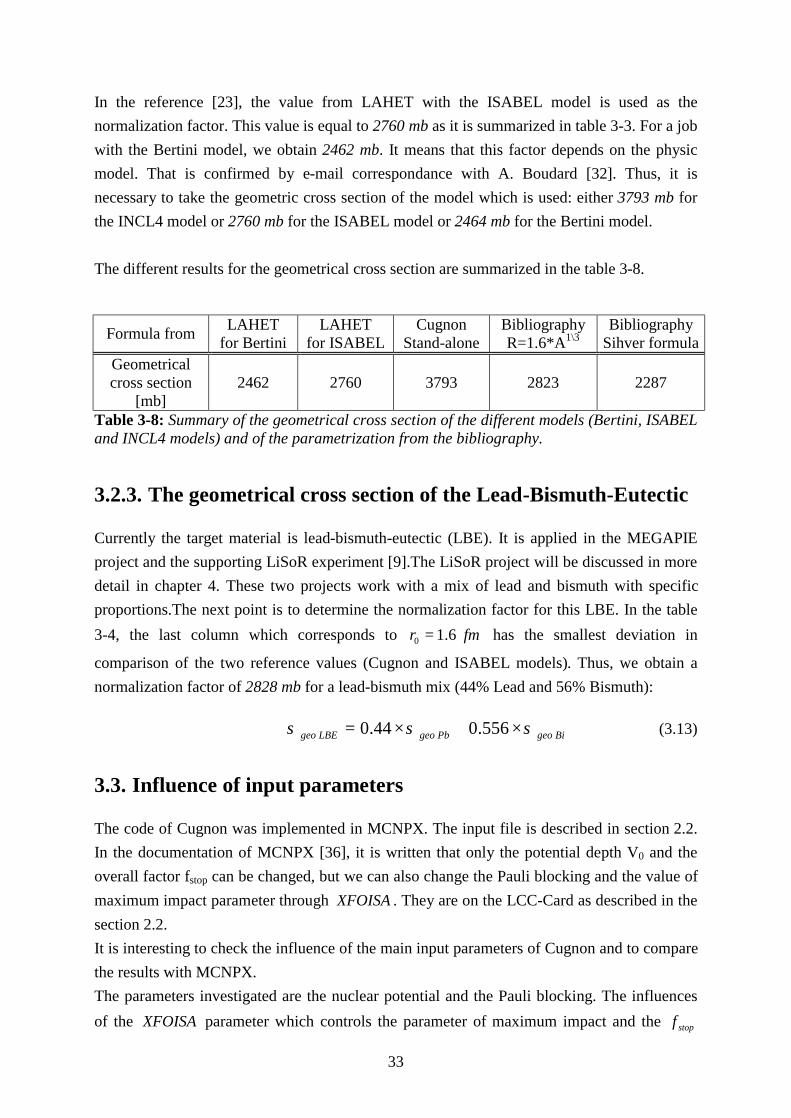
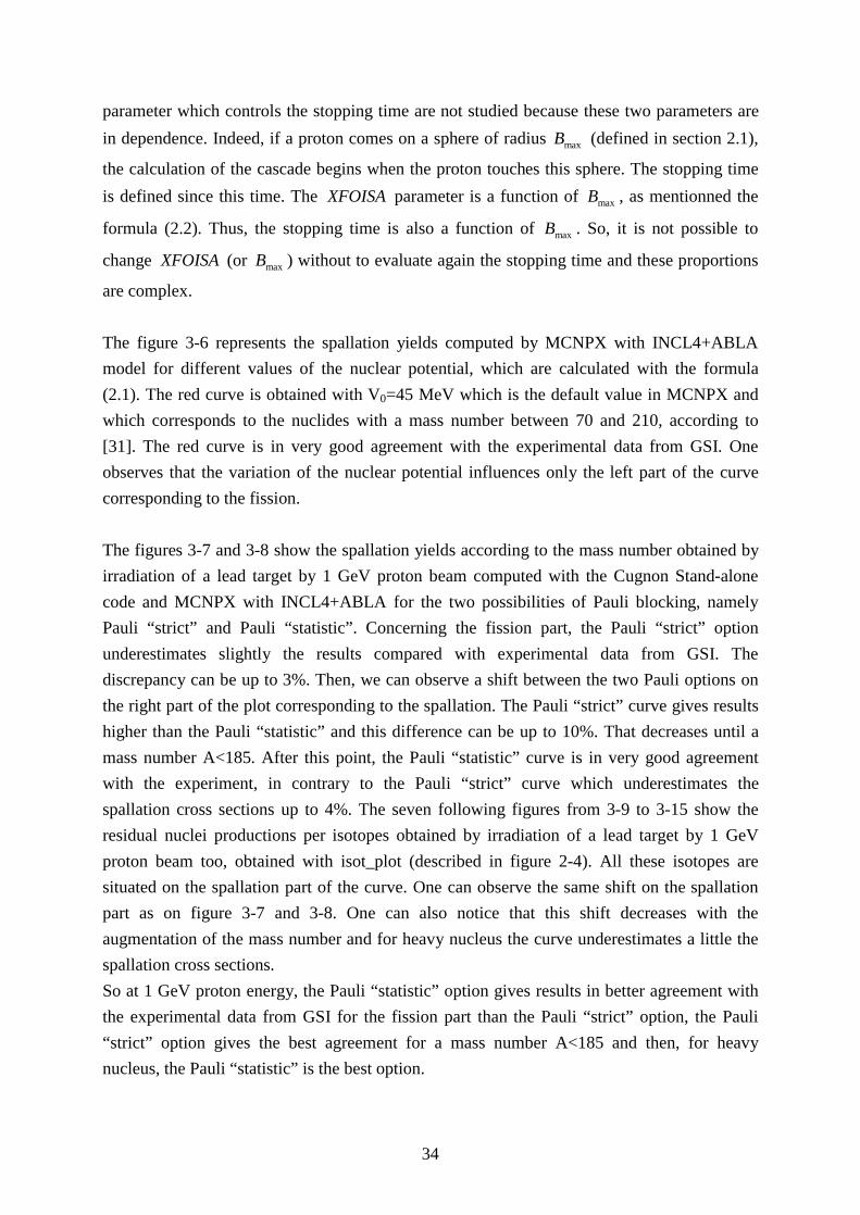
are complex. The figure 3-6 represents the spallation yields computed by MCNPX with INCL4+ABLA model for different values of the nuclear potential, which are calculated with the formula (2.1). The red curve is obtained with V0=45 MeV which is the default value in MCNPX and which corresponds to the nuclides with a mass number between 70 and 210, according to [31]. The red curve is in very good agreement with the experimental data from GSI. One observes that the variation of the nuclear potential influences only the left part of the curve corresponding to the fission. The figures 3-7 and 3-8 show the spallation yields according to the mass number obtained by irradiation of a lead target by 1 GeV proton beam computed with the Cugnon Stand-alone code and MCNPX with INCL4+ABLA for the two possibilities of Pauli blocking, namely Pauli “strict” and Pauli “statistic”. Concerning the fission part, the Pauli “strict” option underestimates slightly the results compared with experimental data from GSI. The discrepancy can be up to 3%. Then, we can observe a shift between the two Pauli options on the right part of the plot corresponding to the spallation. The Pauli “strict” curve gives results higher than the Pauli “statistic” and this difference can be up to 10%. That decreases until a mass number A<185. After this point, the Pauli “statistic” curve is in very good agreement with the experiment, in contrary to the Pauli “strict” curve which underestimates the spallation cross sections up to 4%. The seven following figures from 3-9 to 3-15 show the residual nuclei productions per isotopes obtained by irradiation of a lead target by 1 GeV proton beam too, obtained with isot_plot (described in figure 2-4). All these isotopes are situated on the spallation part of the curve. One can observe the same shift on the spallation part as on figure 3-7 and 3-8. One can also notice that this shift decreases with the augmentation of the mass number and for heavy nucleus the curve underestimates a little the spallation cross sections. So at 1 GeV proton energy, the Pauli “statistic” option gives results in better agreement with the experimental data from GSI for the fission part than the Pauli “strict” option, the Pauli “strict” option gives the best agreement for a mass number A<185 and then, for heavy nucleus, the Pauli “statistic” is the best option.
35
Figure 3-6: Comparison of with MCNPX computed spallation yields (INCL4+ABLA model) for three different value of the nuclear potential and experimental spallation yields (GSI, ISTC). Mass yields in millibarn [mb] as a function of the mass number A.
36
Figure 3-7: Comparison of with MCNPX and the Cugnon code in Stand-alone version computed spallation yields (INCL4+ABLA model) with the Pauli blocking factor set to strict and experimental spallation yields (GSI, ISTC). Mass yields in millibarn [mb] as a function of the mass number A.
37
Figure 3-8: Comparison of with MCNPX and the Cugnon code in Stand-alone version computed spallation yields (INCL4+ABLA model) with the Pauli blocking factor set to statistic and experimental spallation yields (GSI, ISTC). Mass yields in millibarn [mb] as a function of the mass number A.
38
Figure 3-9: Influence of the Pauli blocking factor on the residual nuclei production per isotopes computed with INCL4+ABLA model in MCNPX for isotopes with a charge number between 68 and 70.
39
Figure 3-10: Influence of the Pauli blocking factor on the residual nuclei production per isotopes computed with INCL4+ABLA model in MCNPX for isotopes with a charge number between 70 and 73.
40
Figure 3-11: Influence of the Pauli blocking factor on the residual nuclei production per isotopes computed with INCL4+ABLA model in MCNPX for isotopes with a charge number between 73 and 75.
41
Figure 3-12: Influence of the Pauli blocking factor on the residual nuclei production per isotopes computed with INCL4+ABLA model in MCNPX for isotopes with a charge number between 76 and 77.
42
Figure 3-13: Influence of the Pauli blocking factor on the residual nuclei production per isotopes computed with INCL4+ABLA model in MCNPX for isotopes with a charge number between 78 and 79.
43
Figure 3-14: Influence of the Pauli blocking factor on the residual nuclei production per isotopes computed with INCL4+ABLA model in MCNPX for isotopes with a charge number between 80 and 81.
44
Figure 3-15: Influence of the Pauli blocking factor on the residual nuclei production per isotopes computed with INCL4+ABLA model in MCNPX for isotopes with a charge number between 82 and 83.
45
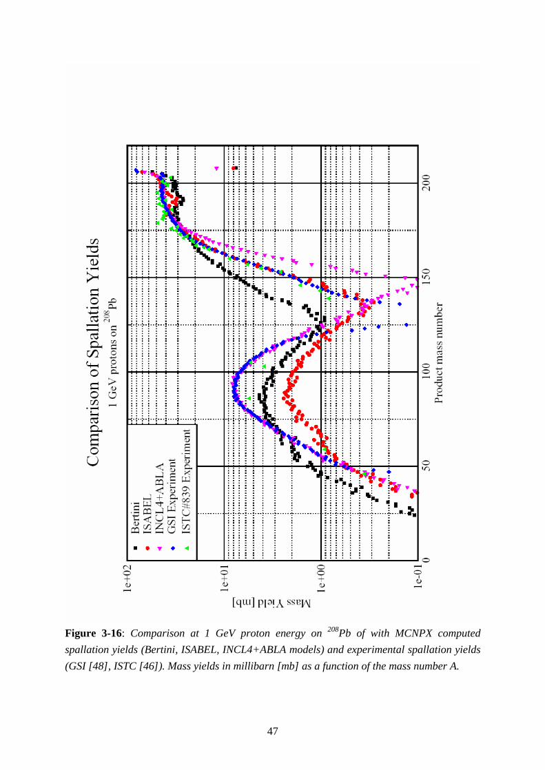
3.4. Thin target experiment at 1 GeV proton energy
3.4.1. Experimental methods The experimental data come from two sources: ISTC [46] and GSI. All the experiments from the GSI group are available in reference [47]. There are also informations about the detector FRS, the experiment, the data and their analysis. There are two different methods to obtain the experimental data: The inverse kinematic and direct proton irradiation. The direct kinematic is the method used at ISTC. The principle is a target irradiated by a proton beam. The benefit of this method is the possibility to use a lot of different targets. But there are also disadvantages: First the nuclei are identified with the gamma-spectroscopy, thus only the nuclei with a half-life larger than half one hour are detected and the stable nuclei are not detected. Secondly, one obtains cumulative cross sections and the results must be analyzed. At the GSI in Darmstadt, it is the inverse kinematics which is applied. A beam of heavy nucleus is projected on a proton target. The proton target is liquid hydrogen at 20 Kelvin. This method gives direct cross section and detects all residual nuclei. The problem is the techniques. Indeed, a high energy accelerator for heavy nucleus is a complex device.
3.4.2. Check of old measurements and validation of the different physical models These comparisons were already done in reference [23]. This section allows us validating again the MCNPX results with the experimental data at 1 GeV proton energy. The correct method and normalization to obtain the spallation yields have been presented in the previous chapter and we can do a new validation of the different model of MCNPX Bertini, ISABEL and add the INCL4+ABLA model. Let us consider now the figure 3-16. It shows the spallation yields of 208Pb computed by MCNPX with the Bertini, ISABEL and INCL4+ABLA models compared to the experimental data at 1 GeV from GSI [48] and ISTC [46]. First of all, one observes that all the models have the same shape of curve as the experimental data. Indeed, there are two distinct parts on the curve: The left part corresponding to the fission and the second right part corresponding to the spallation. The Bertini model gives not very good estimation of the spallation cross sections. This discrepancy can be up to 50%. The ISABEL model is in very good agreement for the spallation part of the curve what corresponds to a mass number A>140 except a cavity for a mass number 186≤A≤198. However, the ISABEL model underestimates a lot the spallation
46
cross sections for the fission part (A<140) and the discrepancy can be up to 70%. Let us consider now the results obtained with the INCL4+ABLA model. Its agreement with the experimental data is very good, especially for the fission part (A<120) and for the spallation part since a mass number A>175. For 120≤A≤137, the INCL4+ABLA model overestimates the spallation cross sections and for 137≤A≤175, it underestimates the results. A good solution for estimating the spallation cross sections would be to use two models:
• For a mass number A<120, we recommend to use the INCL4+ABLA model. • For a mass number 120≤A≤140, there is a hole. All the models give results with a big
difference with the experimental data, but the model which gives the smaller discrepancy is ISABEL. So we recommend it for the small contributions in this range of mass number A.
• For a mass number 140≤A≤186, we recommend to use the ISABEL model. • For a mass number A>186, we recommend to use the INCL4+ABLA model.
47
Figure 3-16: Comparison at 1 GeV proton energy on 208Pb of with MCNPX computed spallation yields (Bertini, ISABEL, INCL4+ABLA models) and experimental spallation yields (GSI [48], ISTC [46]). Mass yields in millibarn [mb] as a function of the mass number A.
48
3.5. Evaluation of new experimental data
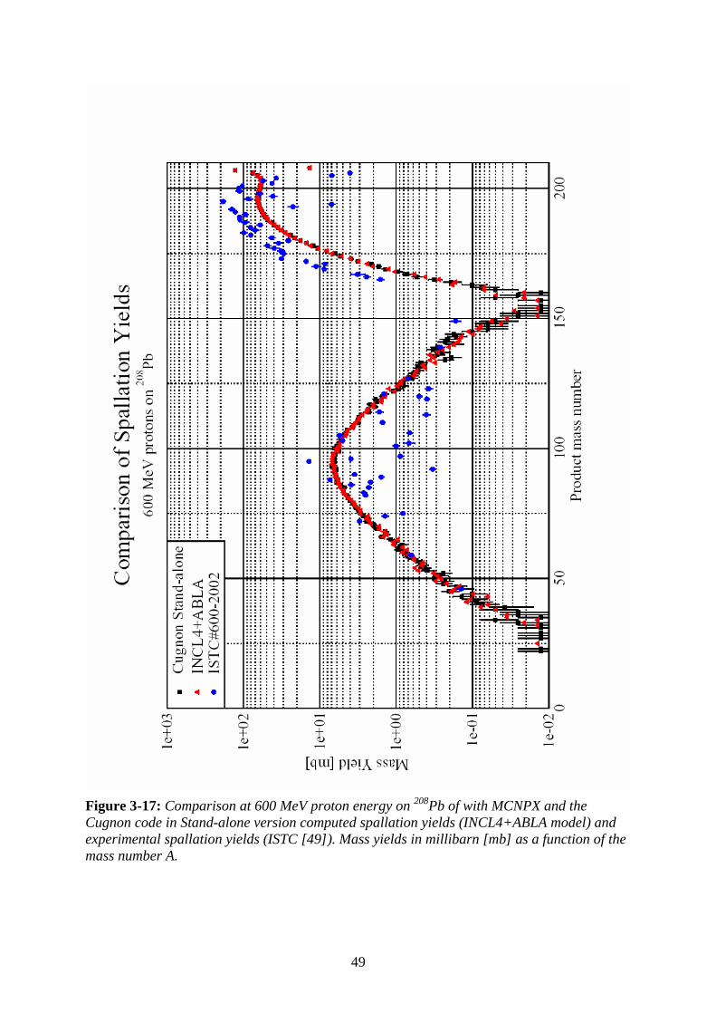
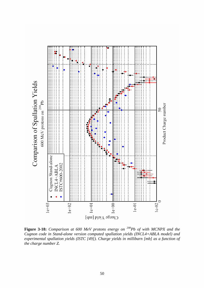
3.5.1. New available data We have obtained preleminary experimental data at 600 MeV from Titarenko in the framework of the ISTC project #2002 [49] (See annex B). The independent yields of a reaction product with mass number A and charge number Z is the probability for the nuclide to be produced directly as a reaction proceeds. The cumulative yield is meant the probability for the nuclide to be produced in all the appropriate processes that can lead to its production. The experimental data show on the figures 3-17 and 3-18 are raw data, which has to be analyzed in more detail. Recently results of 500 MeV experiments with inverse kinematic methods at GSI became available [27, 50]. The fission part [27] and the spallation [50] part are obtained independently.
3.5.2. Thin target experiment at 600 MeV proton energy The figure 3-17 and 3-18 show us the new experimental data at 600 MeV from ISTC project #2002 [49] compared to the spallation cross sections obtained with MCNPX and the Cugnon code in Stand-alone version by irradiation of a 208Pb target at 600 MeV protons beam energy as a function of the mass number A (see figure 3-17) and as a function of the charge number (see figure 3-18) One can observe a significant dispersion of the experimental data, especially for the fission part. It can be explained because it is raw data. As already said in the previous section, this experimental data must be evaluated. The next step is to analyze with more detail this data. However, one can observe that the spallation part has a shape near of the shape of the curve obtaine with the simulation codes.
49
Figure 3-17: Comparison at 600 MeV proton energy on 208Pb of with MCNPX and the Cugnon code in Stand-alone version computed spallation yields (INCL4+ABLA model) and experimental spallation yields (ISTC [49]). Mass yields in millibarn [mb] as a function of the mass number A.
50
Figure 3-18: Comparison at 600 MeV protons energy on 208Pb of with MCNPX and the Cugnon code in Stand-alone version computed spallation yields (INCL4+ABLA model) and experimental spallation yields (ISTC [49]). Charge yields in millibarn [mb] as a function of the charge number Z.
51
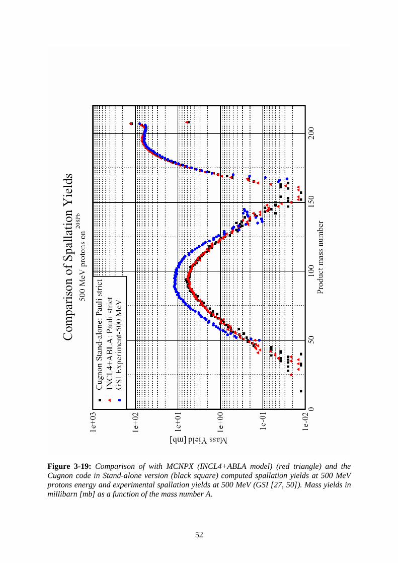
3.5.3. Thin target experiment at 500 MeV proton energy The figure 3-19 shows us this experimental data at 500 MeV compared with the spallation yields computed at 500 MeV with MCNPX (INCL4+ABLA model) and with the Cugnon code in Stand-alone version.
• Comparison on the spallation part of the curve: The results of the two simulation codes with the Pauli “strict” option are in very good agreement with the experiments for the spallation part. There is the same hole for a mass number A≤140 as at 1 GeV protons energy.
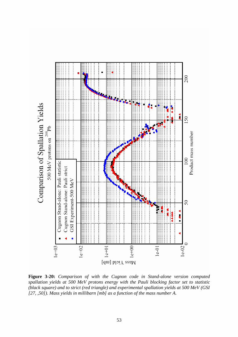
• Comparison on the fission part of the curve: For the fission part, one can observe a difference between the experiment and the simulation. But in reference [27], it is explained that there is a problem with this data. Indeed, these values are higher than the experimental results at 1 GeV. In reference [27], this difference is discussed and a correction is proposed which leads to good agreement with our simulations. The influence of the Pauli blocking at 500 MeV on the spallation yields computed with the Cugnon code in Stand-alone version compared to the experimental data at 500 MeV is shown in figure 3-20. One observes that the red triangle curve corresponding to Pauli strict is in very good agreement with the experimental data. This conclusion is in agreement with the results at 1 GeV where Pauli strict gave also the best agreement with the experimental data from GSI.
52
Figure 3-19: Comparison of with MCNPX (INCL4+ABLA model) (red triangle) and the Cugnon code in Stand-alone version (black square) computed spallation yields at 500 MeV protons energy and experimental spallation yields at 500 MeV (GSI [27, 50]). Mass yields in millibarn [mb] as a function of the mass number A.
53
Figure 3-20: Comparison of with the Cugnon code in Stand-alone version computed spallation yields at 500 MeV protons energy with the Pauli blocking factor set to statistic (black square) and to strict (red triangle) and experimental spallation yields at 500 MeV (GSI [27, ,50]). Mass yields in millibarn [mb] as a function of the mass number A.
54
Chapter 4. LiSoR: A supporting experiment for the
MEGAPIE project
4.1. Description of the LiSoR experiment LiSoR (Liquid metal Solid metal Reaction) is an experimental program, which is supporting the MEGAPIE (1 Megawatt Pilot Experiment) project [1, 10]. The LiSoR experiment simulates the specific MEGAPIE conditions and is a validation step for the MEGAPIE safety assessment and analysis. The purpose is the study of the window damage and the qualification of materials under irradiation and stress and in presence of a flowing molten metal mix (Pb-Bi). Lead-Bismuth-Eutectic (LBE) is the prime candidate to be applied as target material for MEGAPIE due to the low melting point, low vapor pressure and the satisfactory neutron production efficiency. Yet, the compatibility between LBE and structural materials under irradiation and stress has to be proved. The figure 4-1, taken from [51], shows the test tube of the LiSoR experiment.
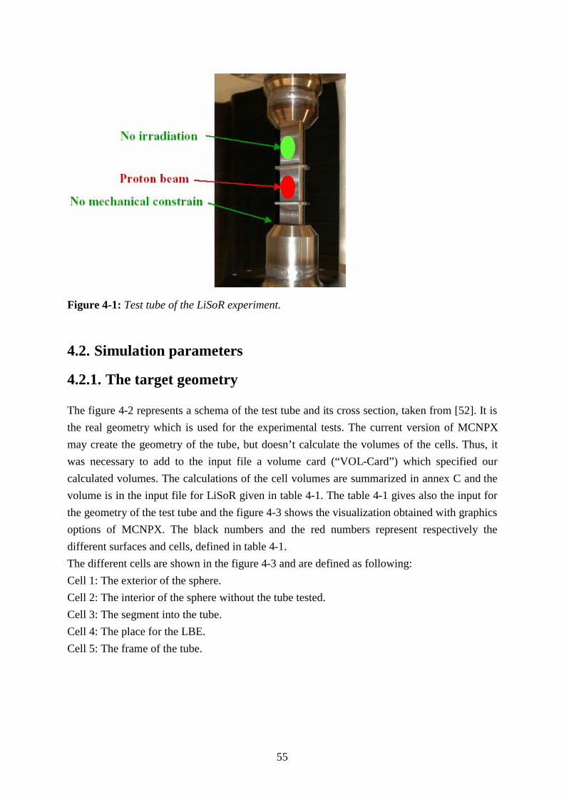
55
Figure 4-1: Test tube of the LiSoR experiment.
4.2. Simulation parameters
4.2.1. The target geometry The figure 4-2 represents a schema of the test tube and its cross section, taken from [52]. It is the real geometry which is used for the experimental tests. The current version of MCNPX may create the geometry of the tube, but doesn’t calculate the volumes of the cells. Thus, it was necessary to add to the input file a volume card (“VOL-Card”) which specified our calculated volumes. The calculations of the cell volumes are summarized in annex C and the volume is in the input file for LiSoR given in table 4-1. The table 4-1 gives also the input for the geometry of the test tube and the figure 4-3 shows the visualization obtained with graphics options of MCNPX. The black numbers and the red numbers represent respectively the different surfaces and cells, defined in table 4-1. The different cells are shown in the figure 4-3 and are defined as following: Cell 1: The exterior of the sphere. Cell 2: The interior of the sphere without the tube tested. Cell 3: The segment into the tube. Cell 4: The place for the LBE. Cell 5: The frame of the tube.
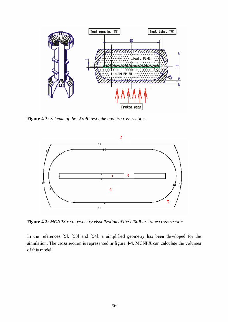
56
Figure 4-2: Schema of the LiSoR test tube and its cross section.
Figure 4-3: MCNPX real geometry visualization of the LiSoR test tube cross section.
In the references [9], [53] and [54], a simplified geometry has been developed for the simulation. The cross section is represented in figure 4-4. MCNPX can calculate the volumes of this model.
4
5
3
2
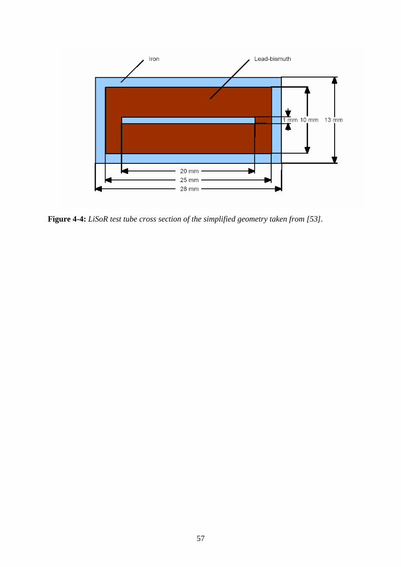
57
Figure 4-4: LiSoR test tube cross section of the simplified geometry taken from [53].
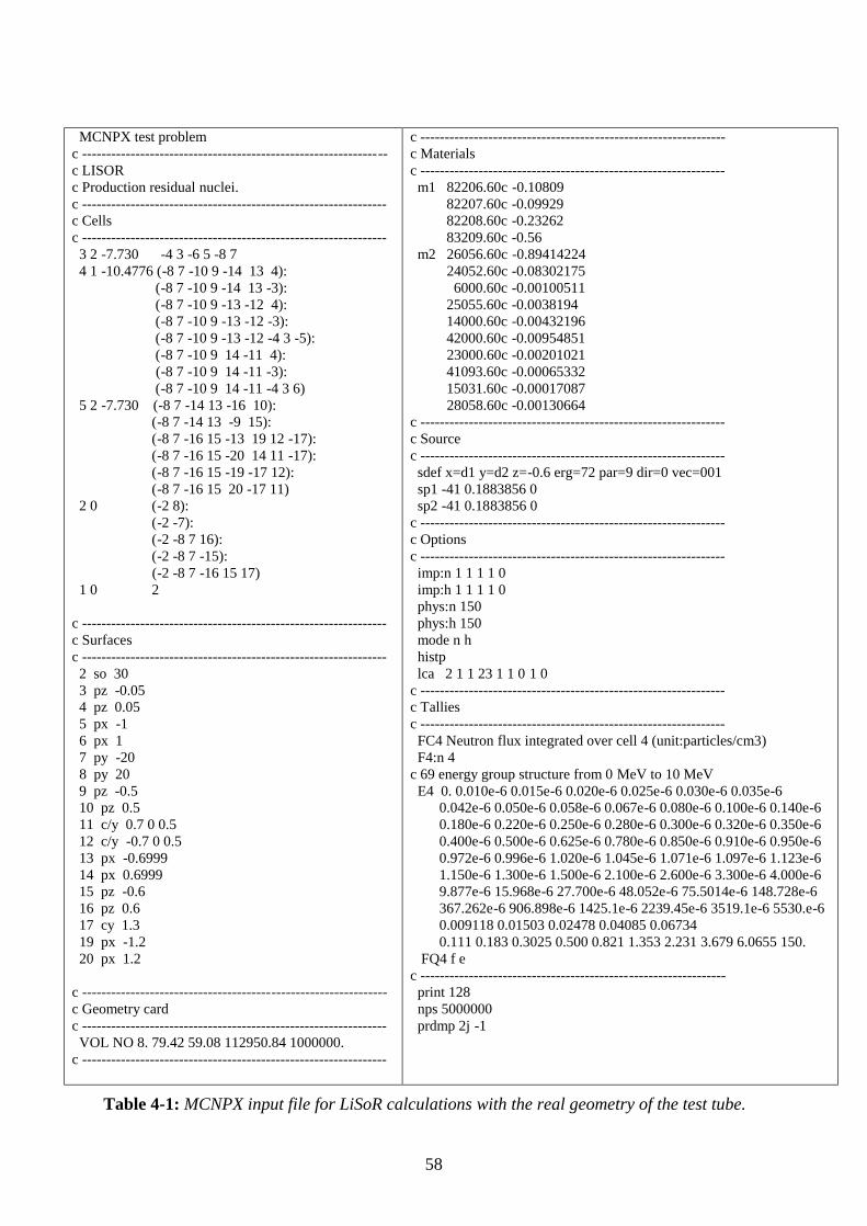
58
MCNPX test problem c --------------------------------------------------------------- c LISOR c Production residual nuclei. c --------------------------------------------------------------- c Cells c --------------------------------------------------------------- 3 2 -7.730 -4 3 -6 5 -8 7 4 1 -10.4776 (-8 7 -10 9 -14 13 4): (-8 7 -10 9 -14 13 -3): (-8 7 -10 9 -13 -12 4): (-8 7 -10 9 -13 -12 -3): (-8 7 -10 9 -13 -12 -4 3 -5): (-8 7 -10 9 14 -11 4): (-8 7 -10 9 14 -11 -3): (-8 7 -10 9 14 -11 -4 3 6) 5 2 -7.730 (-8 7 -14 13 -16 10): (-8 7 -14 13 -9 15): (-8 7 -16 15 -13 19 12 -17): (-8 7 -16 15 -20 14 11 -17): (-8 7 -16 15 -19 -17 12): (-8 7 -16 15 20 -17 11) 2 0 (-2 8): (-2 -7): (-2 -8 7 16): (-2 -8 7 -15): (-2 -8 7 -16 15 17) 1 0 2 c --------------------------------------------------------------- c Surfaces c --------------------------------------------------------------- 2 so 30 3 pz -0.05 4 pz 0.05 5 px -1 6 px 1 7 py -20 8 py 20 9 pz -0.5 10 pz 0.5 11 c/y 0.7 0 0.5 12 c/y -0.7 0 0.5 13 px -0.6999 14 px 0.6999 15 pz -0.6 16 pz 0.6 17 cy 1.3 19 px -1.2 20 px 1.2 c --------------------------------------------------------------- c Geometry card c --------------------------------------------------------------- VOL NO 8. 79.42 59.08 112950.84 1000000. c ---------------------------------------------------------------
c --------------------------------------------------------------- c Materials c --------------------------------------------------------------- m1 82206.60c -0.10809 82207.60c -0.09929 82208.60c -0.23262 83209.60c -0.56 m2 26056.60c -0.89414224 24052.60c -0.08302175 6000.60c -0.00100511 25055.60c -0.0038194 14000.60c -0.00432196 42000.60c -0.00954851 23000.60c -0.00201021 41093.60c -0.00065332 15031.60c -0.00017087 28058.60c -0.00130664 c --------------------------------------------------------------- c Source c --------------------------------------------------------------- sdef x=d1 y=d2 z=-0.6 erg=72 par=9 dir=0 vec=001 sp1 -41 0.1883856 0 sp2 -41 0.1883856 0 c --------------------------------------------------------------- c Options c --------------------------------------------------------------- imp:n 1 1 1 1 0 imp:h 1 1 1 1 0 phys:n 150 phys:h 150 mode n h histp lca 2 1 1 23 1 1 0 1 0 c --------------------------------------------------------------- c Tallies c --------------------------------------------------------------- FC4 Neutron flux integrated over cell 4 (unit:particles/cm3) F4:n 4 c 69 energy group structure from 0 MeV to 10 MeV E4 0. 0.010e-6 0.015e-6 0.020e-6 0.025e-6 0.030e-6 0.035e-6 0.042e-6 0.050e-6 0.058e-6 0.067e-6 0.080e-6 0.100e-6 0.140e-6 0.180e-6 0.220e-6 0.250e-6 0.280e-6 0.300e-6 0.320e-6 0.350e-6 0.400e-6 0.500e-6 0.625e-6 0.780e-6 0.850e-6 0.910e-6 0.950e-6 0.972e-6 0.996e-6 1.020e-6 1.045e-6 1.071e-6 1.097e-6 1.123e-6 1.150e-6 1.300e-6 1.500e-6 2.100e-6 2.600e-6 3.300e-6 4.000e-6 9.877e-6 15.968e-6 27.700e-6 48.052e-6 75.5014e-6 148.728e-6 367.262e-6 906.898e-6 1425.1e-6 2239.45e-6 3519.1e-6 5530.e-6 0.009118 0.01503 0.02478 0.04085 0.06734 0.111 0.183 0.3025 0.500 0.821 1.353 2.231 3.679 6.0655 150. FQ4 f e c --------------------------------------------------------------- print 128 nps 5000000 prdmp 2j -1
Table 4-1: MCNPX input file for LiSoR calculations with the real geometry of the test tube.
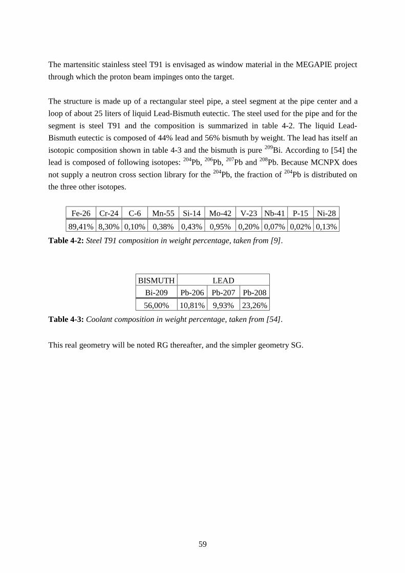
59
The martensitic stainless steel T91 is envisaged as window material in the MEGAPIE project through which the proton beam impinges onto the target. The structure is made up of a rectangular steel pipe, a steel segment at the pipe center and a loop of about 25 liters of liquid Lead-Bismuth eutectic. The steel used for the pipe and for the segment is steel T91 and the composition is summarized in table 4-2. The liquid Lead-Bismuth eutectic is composed of 44% lead and 56% bismuth by weight. The lead has itself an isotopic composition shown in table 4-3 and the bismuth is pure 209Bi. According to [54] the lead is composed of following isotopes: 204Pb, 206Pb, 207Pb and 208Pb. Because MCNPX does not supply a neutron cross section library for the 204Pb, the fraction of 204Pb is distributed on the three other isotopes.
Fe-26 Cr-24 C-6 Mn-55 Si-14 Mo-42 V-23 Nb-41 P-15 Ni-28 89,41% 8,30% 0,10% 0,38% 0,43% 0,95% 0,20% 0,07% 0,02% 0,13%
Table 4-2: Steel T91 composition in weight percentage, taken from [9].
BISMUTH LEAD Bi-209 Pb-206 Pb-207 Pb-208 56,00% 10,81% 9,93% 23,26%
Table 4-3: Coolant composition in weight percentage, taken from [54]. This real geometry will be noted RG thereafter, and the simpler geometry SG.
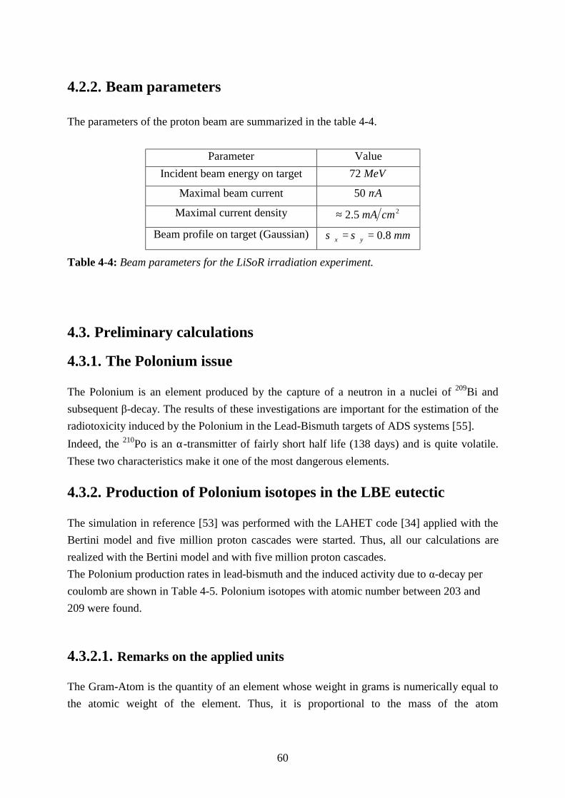
60
4.2.2. Beam parameters The parameters of the proton beam are summarized in the table 4-4.
Parameter Value Incident beam energy on target MeV72
Maximal beam current Aµ50
Maximal current density 25.2 cmmA≈
Beam profile on target (Gaussian) mmyx 8.0== σσ
Table 4-4: Beam parameters for the LiSoR irradiation experiment.
4.3. Preliminary calculations
4.3.1. The Polonium issue The Polonium is an element produced by the capture of a neutron in a nuclei of 209Bi and subsequent β-decay. The results of these investigations are important for the estimation of the radiotoxicity induced by the Polonium in the Lead-Bismuth targets of ADS systems [55]. Indeed, the 210Po is an α-transmitter of fairly short half life (138 days) and is quite volatile. These two characteristics make it one of the most dangerous elements.
4.3.2. Production of Polonium isotopes in the LBE eutectic The simulation in reference [53] was performed with the LAHET code [34] applied with the Bertini model and five million proton cascades were started. Thus, all our calculations are realized with the Bertini model and with five million proton cascades. The Polonium production rates in lead-bismuth and the induced activity due to α-decay per coulomb are shown in Table 4-5. Polonium isotopes with atomic number between 203 and 209 were found.
4.3.2.1. Remarks on the applied units The Gram-Atom is the quantity of an element whose weight in grams is numerically equal to the atomic weight of the element. Thus, it is proportional to the mass of the atom
61
corresponding and the factor of proportionality is the number of Avogadro AN . For example,
1 Gram-Atom of Carbon 12 will be 12 Grams of pure Carbon 12. The mole is the unit of quantity of material equivalent to the sum of the Gram-Atom of the elements composing it. The Coulomb is a unit of electrical charge equal to the amount of charge transferred by a current of 1 ampere in 1 second
The Becquerel is the standard international unit of radioactive decay and it is represented as one disintegration per second. The units utilised by the PSI in [9] and [52] are:
•
Coulomb
Atoms for the initial production rate.
• [ ]literAtomGram. for the intermediate production rate utilised for the calculation related to
the decay of the Polonium isotopes.
•
CoulombBecquerel and [ ]Bq for the α-activity.
The production rates come from the file opt8a generated by MCNPX and HTAPE3X. The program CRORINP changes the units and creates an adapted file for ORIHET3. For the later use of the small auxilliary program CRORINP (see figure 5-3), it is important to note that the average beam current is an intern constant in this program and that it is necessary to change it within an application for MEGAPIE or LiSoR as example.
4.3.2.2. Calculation of radioactivity The first step will be to show how to calculate the induced α-activity at the end of the irradiation. It can be written as:
0PRKA ××= αα λ (4.1)
where αA is the α-activity in
CoulombBecquerel .
λ is the decay constants in [ ]1−s .
0PR is the initial production rate in
Coulomb
Atoms .
αK is the branching ratio for the α-activity in [ ]% . The values of this branching ratio for the α-activity are taken from [56]
62
The decay constants λ are calculated as following:
( )
21
2lnT
=λ (4.2)
where
21T is the half-life in [ ]s .
The next step is to show how to calculate the decay of the nuclei. The time dependent evolution of the number of unstable nuclei can be written as:
( ) teNtN λ−= 0 (4.3) where 0N is the number of atoms of unstable nuclei existing at the end of the irradiation. The number of decay corresponding to the production rate is:
( ) ( ) ( )teNtNNtD λ−−=−= 100 (4.4) where ( )tD is the number of atoms of unstable nuclei at the time t after the end of the irradiation.
The following formula allows calculating the production rate in
literAtomGram. at different
times after the end of the irradiation, taken into account the appropriate dimension conversions, to compare directly with the results of [53]:
( ) ( )( )t
A
ePRVN
ItPR λ
λ−−×
××= 10 (4.5)
where ( )tPR is the production rate at the time t in
literAtomGram. .
0PR is the initial production rate in
Coulomb
Atoms .
AAI 610.5050 −== µ is the average beam current during the irradiation.
AtomGram
AtomsN A .10.022.6 23= is the Avogadro’s number.
lV 25= is the volume of eutectic of the LiSoR experiment. Moreover:
( ) ( ) ANKVtPRtA ××××= αα λ (4.6)
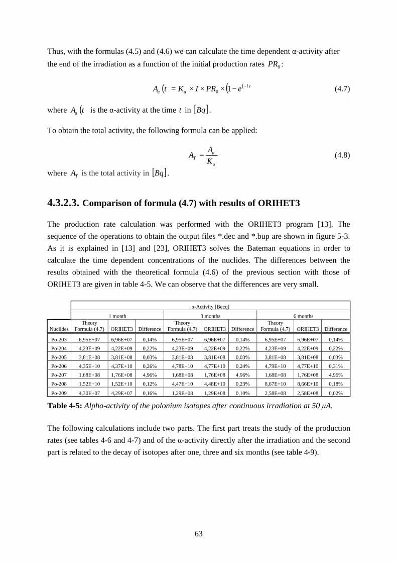
63
Thus, with the formulas (4.5) and (4.6) we can calculate the time dependent α-activity after the end of the irradiation as a function of the initial production rates 0PR :
( ) ( )( )tePRIKtA λ
αα−−×××= 10 (4.7)
where ( )tAα is the α-activity at the time t in [ ]Bq . To obtain the total activity, the following formula can be applied:
α
α
KA
AT = (4.8)
where TA is the total activity in [ ]Bq .
4.3.2.3. Comparison of formula (4.7) with results of ORIHET3 The production rate calculation was performed with the ORIHET3 program [13]. The sequence of the operations to obtain the output files *.dec and *.bup are shown in figure 5-3. As it is explained in [13] and [23], ORIHET3 solves the Bateman equations in order to calculate the time dependent concentrations of the nuclides. The differences between the results obtained with the theoretical formula (4.6) of the previous section with those of ORIHET3 are given in table 4-5. We can observe that the differences are very small. α-Activity [Becq]
1 month 3 months 6 months
Nuclides Theory
Formula (4.7) ORIHET3 Difference Theory
Formula (4.7) ORIHET3 Difference Theory
Formula (4.7) ORIHET3 Difference
Po-203 6,95E+07 6,96E+07 0,14% 6,95E+07 6,96E+07 0,14% 6,95E+07 6,96E+07 0,14% Po-204 4,23E+09 4,22E+09 0,22% 4,23E+09 4,22E+09 0,22% 4,23E+09 4,22E+09 0,22%
Po-205 3,81E+08 3,81E+08 0,03% 3,81E+08 3,81E+08 0,03% 3,81E+08 3,81E+08 0,03% Po-206 4,35E+10 4,37E+10 0,26% 4,78E+10 4,77E+10 0,24% 4,79E+10 4,77E+10 0,31% Po-207 1,68E+08 1,76E+08 4,96% 1,68E+08 1,76E+08 4,96% 1,68E+08 1,76E+08 4,96%
Po-208 1,52E+10 1,52E+10 0,12% 4,47E+10 4,48E+10 0,23% 8,67E+10 8,66E+10 0,18%
Po-209 4,30E+07 4,29E+07 0,16% 1,29E+08 1,29E+08 0,10% 2,58E+08 2,58E+08 0,02%
Table 4-5: Alpha-activity of the polonium isotopes after continuous irradiation at 50 μA.
The following calculations include two parts. The first part treats the study of the production rates (see tables 4-6 and 4-7) and of the α-activity directly after the irradiation and the second part is related to the decay of isotopes after one, three and six months (see table 4-9).
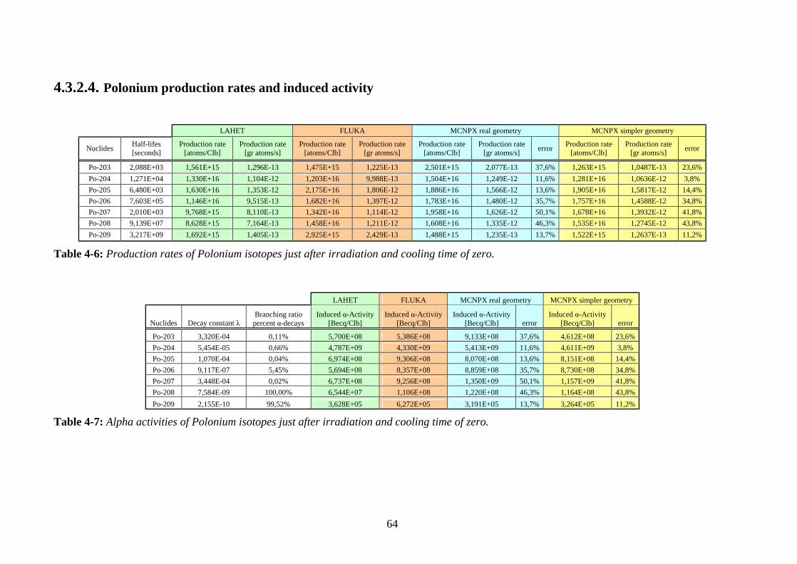
64
4.3.2.4. Polonium production rates and induced activity
LAHET FLUKA MCNPX real geometry MCNPX simpler geometry
Nuclides Half-lifes [seconds]
Production rate [atoms/Clb]
Production rate [gr atoms/s]
Production rate [atoms/Clb]
Production rate [gr atoms/s]
Production rate [atoms/Clb]
Production rate [gr atoms/s] error Production rate
[atoms/Clb] Production rate
[gr atoms/s] error
Po-203 2,088E+03 1,561E+15 1,296E-13 1,475E+15 1,225E-13 2,501E+15 2,077E-13 37,6% 1,263E+15 1,0487E-13 23,6% Po-204 1,271E+04 1,330E+16 1,104E-12 1,203E+16 9,988E-13 1,504E+16 1,249E-12 11,6% 1,281E+16 1,0636E-12 3,8% Po-205 6,480E+03 1,630E+16 1,353E-12 2,175E+16 1,806E-12 1,886E+16 1,566E-12 13,6% 1,905E+16 1,5817E-12 14,4% Po-206 7,603E+05 1,146E+16 9,515E-13 1,682E+16 1,397E-12 1,783E+16 1,480E-12 35,7% 1,757E+16 1,4588E-12 34,8% Po-207 2,010E+03 9,768E+15 8,110E-13 1,342E+16 1,114E-12 1,958E+16 1,626E-12 50,1% 1,678E+16 1,3932E-12 41,8% Po-208 9,139E+07 8,628E+15 7,164E-13 1,458E+16 1,211E-12 1,608E+16 1,335E-12 46,3% 1,535E+16 1,2745E-12 43,8% Po-209 3,217E+09 1,692E+15 1,405E-13 2,925E+15 2,429E-13 1,488E+15 1,235E-13 13,7% 1,522E+15 1,2637E-13 11,2%
Table 4-6: Production rates of Polonium isotopes just after irradiation and cooling time of zero.
LAHET FLUKA MCNPX real geometry MCNPX simpler geometry
Nuclides Decay constant λ Branching ratio
percent α-decays Induced α-Activity
[Becq/Clb] Induced α-Activity
[Becq/Clb] Induced α-Activity
[Becq/Clb] error Induced α-Activity
[Becq/Clb] error
Po-203 3,320E-04 0,11% 5,700E+08 5,386E+08 9,133E+08 37,6% 4,612E+08 23,6% Po-204 5,454E-05 0,66% 4,787E+09 4,330E+09 5,413E+09 11,6% 4,611E+09 3,8% Po-205 1,070E-04 0,04% 6,974E+08 9,306E+08 8,070E+08 13,6% 8,151E+08 14,4% Po-206 9,117E-07 5,45% 5,694E+08 8,357E+08 8,859E+08 35,7% 8,730E+08 34,8% Po-207 3,448E-04 0,02% 6,737E+08 9,256E+08 1,350E+09 50,1% 1,157E+09 41,8% Po-208 7,584E-09 100,00% 6,544E+07 1,106E+08 1,220E+08 46,3% 1,164E+08 43,8% Po-209 2,155E-10 99,52% 3,628E+05 6,272E+05 3,191E+05 13,7% 3,264E+05 11,2%
Table 4-7: Alpha activities of Polonium isotopes just after irradiation and cooling time of zero.
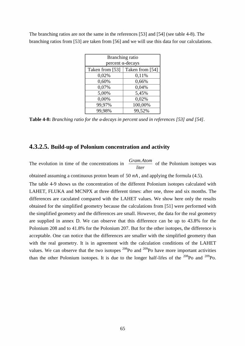
65
The branching ratios are not the same in the references [53] and [54] (see table 4-8). The branching ratios from [53] are taken from [56] and we will use this data for our calculations.
Branching ratio
percent α-decays Taken from [53] Taken from [54]
0,02% 0,11% 0,60% 0,66% 0,07% 0,04% 5,00% 5,45% 0,00% 0,02% 99,97% 100,00% 99,98% 99,52%
Table 4-8: Branching ratio for the α-decays in percent used in references [53] and [54].
4.3.2.5. Build-up of Polonium concentration and activity
The evolution in time of the concentrations in
literAtomGram. of the Polonium isotopes was
obtained assuming a continuous proton beam of Aµ50 , and applying the formula (4.5).
The table 4-9 shows us the concentration of the different Polonium isotopes calculated with LAHET, FLUKA and MCNPX at three different times: after one, three and six months. The differences are caculated compared with the LAHET values. We show here only the results obtained for the simplified geometry because the calculations from [51] were performed with the simplified geometry and the differences are small. However, the data for the real geometry are supplied in annex D. We can observe that this difference can be up to 43.8% for the Polonium 208 and to 41.8% for the Polonium 207. But for the other isotopes, the difference is acceptable. One can notice that the differences are smaller with the simplified geometry than with the real geometry. It is in agreement with the calculation conditions of the LAHET values. We can observe that the two isotopes 208Po and 209Po have more important activities than the other Polonium isotopes. It is due to the longer half-lifes of the 208Po and 209Po.
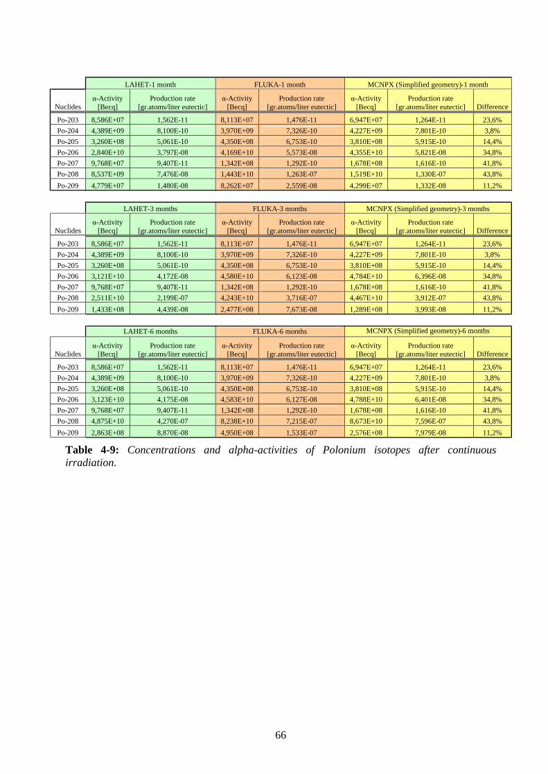
66
LAHET-1 month FLUKA-1 month MCNPX (Simplified geometry)-1 month
Nuclides α-Activity
[Becq] Production rate
[gr.atoms/liter eutectic] α-Activity
[Becq] Production rate
[gr.atoms/liter eutectic] α-Activity
[Becq] Production rate
[gr.atoms/liter eutectic] Difference
Po-203 8,586E+07 1,562E-11 8,113E+07 1,476E-11 6,947E+07 1,264E-11 23,6% Po-204 4,389E+09 8,100E-10 3,970E+09 7,326E-10 4,227E+09 7,801E-10 3,8% Po-205 3,260E+08 5,061E-10 4,350E+08 6,753E-10 3,810E+08 5,915E-10 14,4% Po-206 2,840E+10 3,797E-08 4,169E+10 5,573E-08 4,355E+10 5,821E-08 34,8% Po-207 9,768E+07 9,407E-11 1,342E+08 1,292E-10 1,678E+08 1,616E-10 41,8% Po-208 8,537E+09 7,476E-08 1,443E+10 1,263E-07 1,519E+10 1,330E-07 43,8% Po-209 4,779E+07 1,480E-08 8,262E+07 2,559E-08 4,299E+07 1,332E-08 11,2%
LAHET-3 months FLUKA-3 months MCNPX (Simplified geometry)-3 months
Nuclides α-Activity
[Becq] Production rate
[gr.atoms/liter eutectic] α-Activity
[Becq] Production rate
[gr.atoms/liter eutectic] α-Activity
[Becq] Production rate
[gr.atoms/liter eutectic] Difference
Po-203 8,586E+07 1,562E-11 8,113E+07 1,476E-11 6,947E+07 1,264E-11 23,6% Po-204 4,389E+09 8,100E-10 3,970E+09 7,326E-10 4,227E+09 7,801E-10 3,8% Po-205 3,260E+08 5,061E-10 4,350E+08 6,753E-10 3,810E+08 5,915E-10 14,4% Po-206 3,121E+10 4,172E-08 4,580E+10 6,123E-08 4,784E+10 6,396E-08 34,8% Po-207 9,768E+07 9,407E-11 1,342E+08 1,292E-10 1,678E+08 1,616E-10 41,8% Po-208 2,511E+10 2,199E-07 4,243E+10 3,716E-07 4,467E+10 3,912E-07 43,8% Po-209 1,433E+08 4,439E-08 2,477E+08 7,673E-08 1,289E+08 3,993E-08 11,2%
LAHET-6 months FLUKA-6 months MCNPX (Simplified geometry)-6 months
Nuclides α-Activity
[Becq] Production rate
[gr.atoms/liter eutectic] α-Activity
[Becq] Production rate
[gr.atoms/liter eutectic] α-Activity
[Becq] Production rate
[gr.atoms/liter eutectic] Difference
Po-203 8,586E+07 1,562E-11 8,113E+07 1,476E-11 6,947E+07 1,264E-11 23,6% Po-204 4,389E+09 8,100E-10 3,970E+09 7,326E-10 4,227E+09 7,801E-10 3,8% Po-205 3,260E+08 5,061E-10 4,350E+08 6,753E-10 3,810E+08 5,915E-10 14,4% Po-206 3,123E+10 4,175E-08 4,583E+10 6,127E-08 4,788E+10 6,401E-08 34,8% Po-207 9,768E+07 9,407E-11 1,342E+08 1,292E-10 1,678E+08 1,616E-10 41,8% Po-208 4,875E+10 4,270E-07 8,238E+10 7,215E-07 8,673E+10 7,596E-07 43,8% Po-209 2,863E+08 8,870E-08 4,950E+08 1,533E-07 2,576E+08 7,979E-08 11,2%
Table 4-9: Concentrations and alpha-activities of Polonium isotopes after continuous irradiation.
67
4.4. Calculations related to the LiSoR experimental results The experimental data [57] are measured in the spallation neutron facility SINQ at PSI [58, 59].
Total activity [Bq]
Nuclides LAHET FLUKA
Simplier geometry FLUKA
real geometry MCNPX
Simpler geometry MCNPX
real geometry Experiment
PSI
Po-203 7,805E+10 7,375E+10 2,30E+11 6,315E+10 1,251E+11 Po-204 6,642E+11 6,007E+11 9,90E+11 6,397E+11 7,511E+11
Po-205 8,150E+11 1,087E+12 1,10E+12 9,525E+11 9,430E+11 Po-206 6,050E+10 8,880E+10 9,10E+10 9,276E+10 9,413E+10 1,87E+11
Po-207 4,884E+11 6,710E+11 7,90E+11 8,390E+11 9,790E+11 Po-208 4,003E+08 6,764E+08 5,90E+08 7,122E+08 7,460E+08 9,02E+08
Po-209 2,231E+06 3,857E+06 2,007E+06 1,962E+06
Po-206/Po-208 1,511E+02 1,313E+02 1,54E+02 1,302E+02 1,262E+02 2,07E+02
Table 4-10: Total activity of the Polonium isotopes for several simulations codes and for the experiment.
Total activity of Polonium isostopes
1,E+08
1,E+09
1,E+10
1,E+11
1,E+12
1,E+13
Po-203 Po-204 Po-205 Po-206 Po-207 Po-208 Po-209*100
Nuclide
Tota
l act
ivity
[Bq] LAHET
FLUKA SGFLUKA RGMCNPX SGMCNPX RGExperiment PSI
Figure 4-5: Comparison of the total activity of the Polonium isotopes directly after 34 hours irradiation.
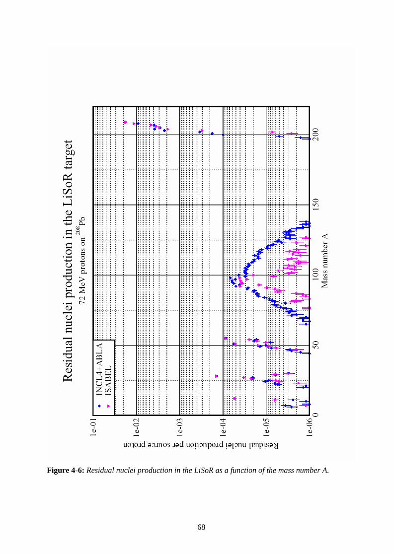
68
Figure 4-6: Residual nuclei production in the LiSoR as a function of the mass number A.
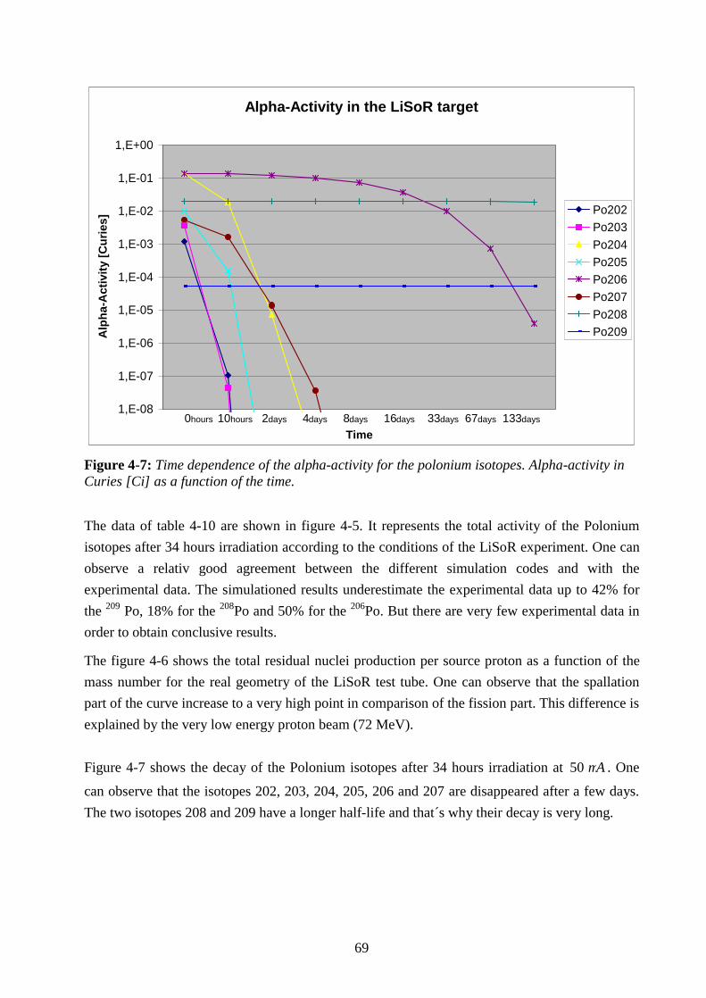
69
Alpha-Activity in the LiSoR target
1,E-08
1,E-07
1,E-06
1,E-05
1,E-04
1,E-03
1,E-02
1,E-01
1,E+00
Time
Alp
ha-A
ctiv
ity [C
urie
s]
Po202Po203Po204Po205Po206Po207Po208Po209
0hours 10hours 2days 4days 8days 16days 33days 67days 133days
Figure 4-7: Time dependence of the alpha-activity for the polonium isotopes. Alpha-activity in Curies [Ci] as a function of the time.
The data of table 4-10 are shown in figure 4-5. It represents the total activity of the Polonium isotopes after 34 hours irradiation according to the conditions of the LiSoR experiment. One can observe a relativ good agreement between the different simulation codes and with the experimental data. The simulationed results underestimate the experimental data up to 42% for the 209 Po, 18% for the 208Po and 50% for the 206Po. But there are very few experimental data in order to obtain conclusive results.
The figure 4-6 shows the total residual nuclei production per source proton as a function of the mass number for the real geometry of the LiSoR test tube. One can observe that the spallation part of the curve increase to a very high point in comparison of the fission part. This difference is explained by the very low energy proton beam (72 MeV). Figure 4-7 shows the decay of the Polonium isotopes after 34 hours irradiation at Aµ50 . One
can observe that the isotopes 202, 203, 204, 205, 206 and 207 are disappeared after a few days. The two isotopes 208 and 209 have a longer half-life and that´s why their decay is very long.
70
Chapter 5. Comparison KAPROS/ORIHET3
5.1. KAPROS
5.1.1. Theory The burn-up equations are described in [11] and are solved with the program BURNUP [12]. With the burn-up code one investigates the time dependent change of the atomic density of a nuclide N. Changes result from the depletion and the production. The production of a nuclide may occur through the following ways:
• Decay other nuclides. • Neutron capture (to which here also (n, 2n) - and (n, 3n) - reaction is counted) of
other nuclides. • Creation of fission products by fission.
The reduction of the isotope number density of a nuclide can take place via the following reactions:
• Decay of this nuclides. • Neutron capture (to which here also (n, 2n) - and (n, 3n) - reactions are counted)
of this nuclide. • Fission.
The time dependence of the nuclide density described by the balance of production and loss rates for each individual nuclide is shown in the following formula:
( ) i
M
kiikkkijj
M
jji
i NNfNldt
dN ∑∑==
Φ+−Φ+=1
,1
, σλσλ (5.1)
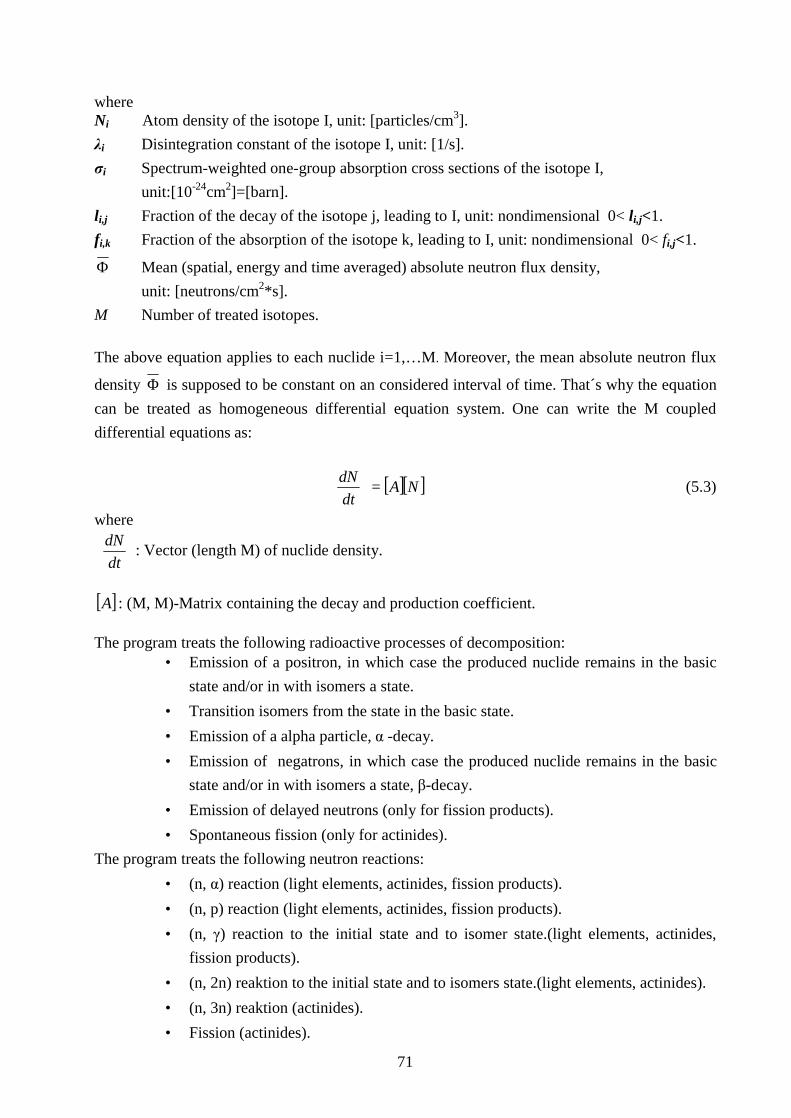
71
where Ni Atom density of the isotope I, unit: [particles/cm3]. λi Disintegration constant of the isotope I, unit: [1/s]. σi Spectrum-weighted one-group absorption cross sections of the isotope I, unit:[10-24cm2]=[barn]. li,j Fraction of the decay of the isotope j, leading to I, unit: nondimensional 0< li,j<1. fi,k Fraction of the absorption of the isotope k, leading to I, unit: nondimensional 0< fi,j<1.
Φ Mean (spatial, energy and time averaged) absolute neutron flux density, unit: [neutrons/cm2*s]. M Number of treated isotopes. The above equation applies to each nuclide i=1,…M. Moreover, the mean absolute neutron flux
density Φ is supposed to be constant on an considered interval of time. That´s why the equation can be treated as homogeneous differential equation system. One can write the M coupled differential equations as:
[ ][ ]NAdtdN
=
(5.3)
where
dtdN : Vector (length M) of nuclide density.
[ ]A : (M, M)-Matrix containing the decay and production coefficient. The program treats the following radioactive processes of decomposition:
• Emission of a positron, in which case the produced nuclide remains in the basic state and/or in with isomers a state.
• Transition isomers from the state in the basic state. • Emission of a alpha particle, α -decay. • Emission of negatrons, in which case the produced nuclide remains in the basic
state and/or in with isomers a state, β-decay. • Emission of delayed neutrons (only for fission products). • Spontaneous fission (only for actinides).
The program treats the following neutron reactions: • (n, α) reaction (light elements, actinides, fission products). • (n, p) reaction (light elements, actinides, fission products). • (n, γ) reaction to the initial state and to isomer state.(light elements, actinides,
fission products). • (n, 2n) reaktion to the initial state and to isomers state.(light elements, actinides). • (n, 3n) reaktion (actinides). • Fission (actinides).

72
At the time of the decomposition of actinides, the formation of the fission products is treated only for one limited number (currently the maximum is 5) of actinides in the program. It depends also on the considered reactor type (NLIBE=1,2,3,4). The library is a reformatted KORIGEN [60] library. The BURNUP modul is developed from the Oak Ridge Code ORIGEN [61]. That’s why the method for the numerical solution is the same. The transition matrix is built from the data of three specific libraries. The first contains the data for decay and activation for light elements, the second data for actinides and the third data for fission products
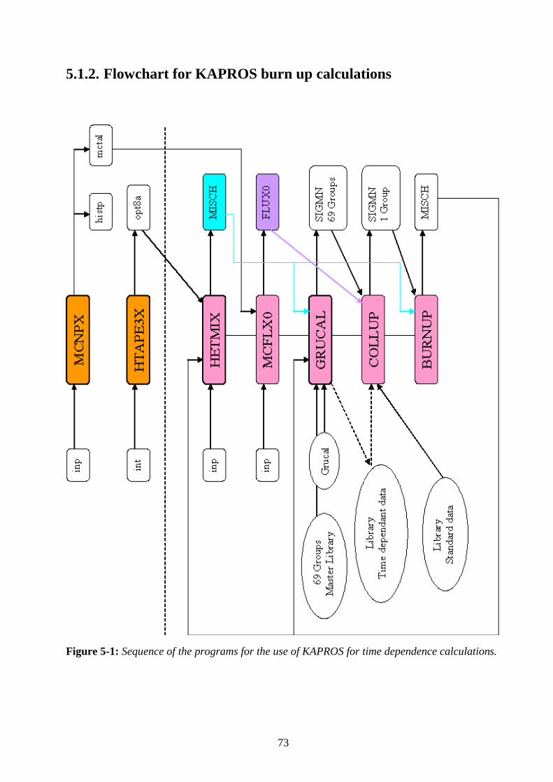
73
5.1.2. Flowchart for KAPROS burn up calculations
Figure 5-1: Sequence of the programs for the use of KAPROS for time dependence calculations.
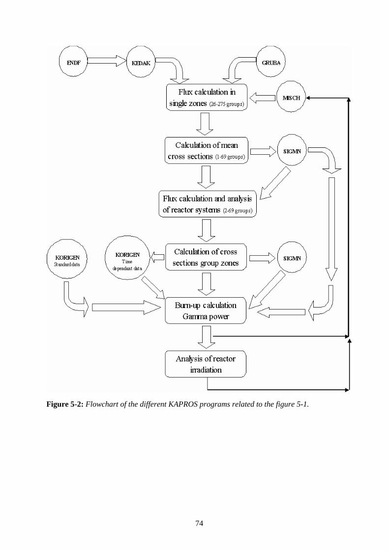
74
Figure 5-2: Flowchart of the different KAPROS programs related to the figure 5-1.
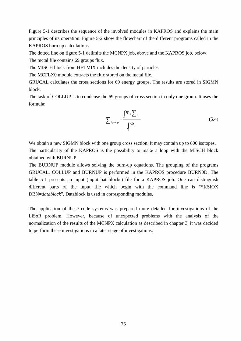
75
Figure 5-1 describes the sequence of the involved modules in KAPROS and explains the main principles of its operation. Figure 5-2 show the flowchart of the different programs called in the KAPROS burn up calculations. The dotted line on figure 5-1 delimits the MCNPX job, above and the KAPROS job, below. The mctal file contains 69 groups flux. The MISCH block from HETMIX includes the density of particles The MCFLX0 module extracts the flux stored on the mctal file. GRUCAL calculates the cross sections for 69 energy groups. The results are stored in SIGMN block. The task of COLLUP is to condense the 69 groups of cross section in only one group. It uses the formula:
∫
∫ ∑∑
Φ
Φ=
ii
iii
group1 (5.4)
We obtain a new SIGMN block with one group cross section. It may contain up to 800 isotopes. The particularity of the KAPROS is the possibility to make a loop with the MISCH block obtained with BURNUP. The BURNUP module allows solving the burn-up equations. The grouping of the programs GRUCAL, COLLUP and BURNUP is performed in the KAPROS procedure BURN0D. The table 5-1 presents an input (input batablocks) file for a KAPROS job. One can distinguish different parts of the input file which begin with the command line is “*KSIOX DBN=datablock”. Datablock is used in corresponding modules. The application of these code systems was prepared more detailed for investigations of the LiSoR problem. However, because of unexpected problems with the analysis of the normalization of the results of the MCNPX calculation as described in chapter 3, it was decided to perform these investigations in a later stage of investigations.
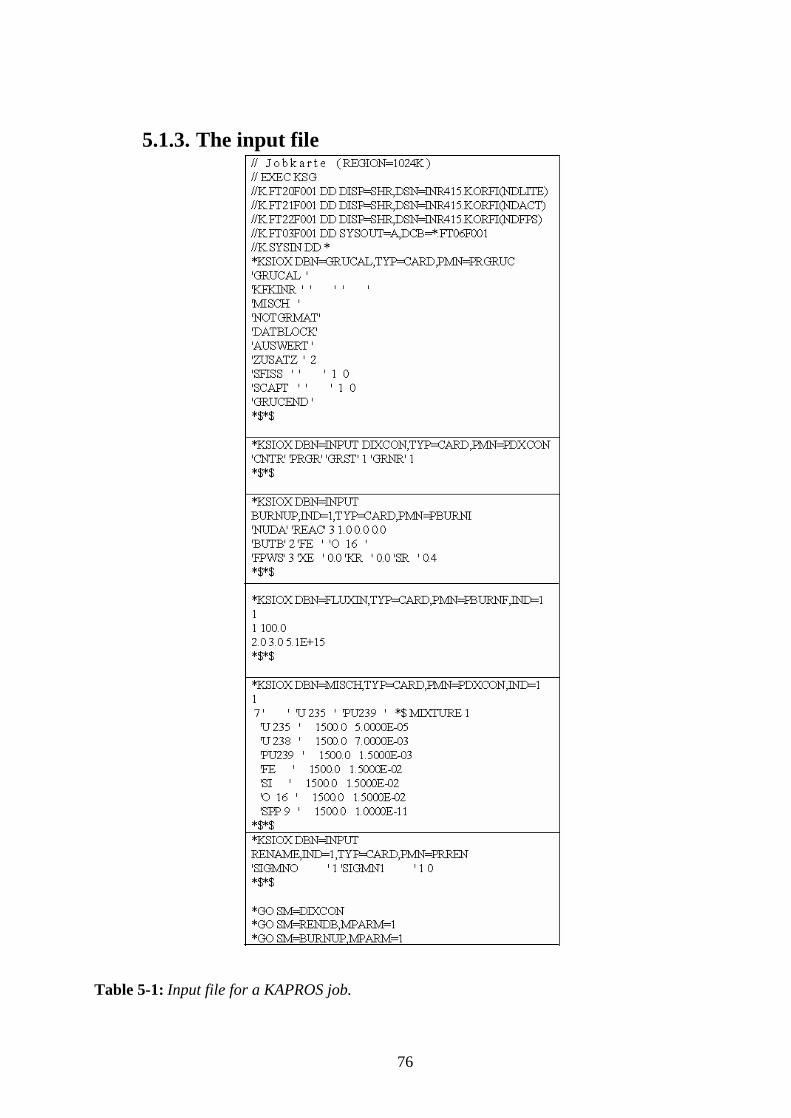
76
5.1.3. The input file
Table 5-1: Input file for a KAPROS job.
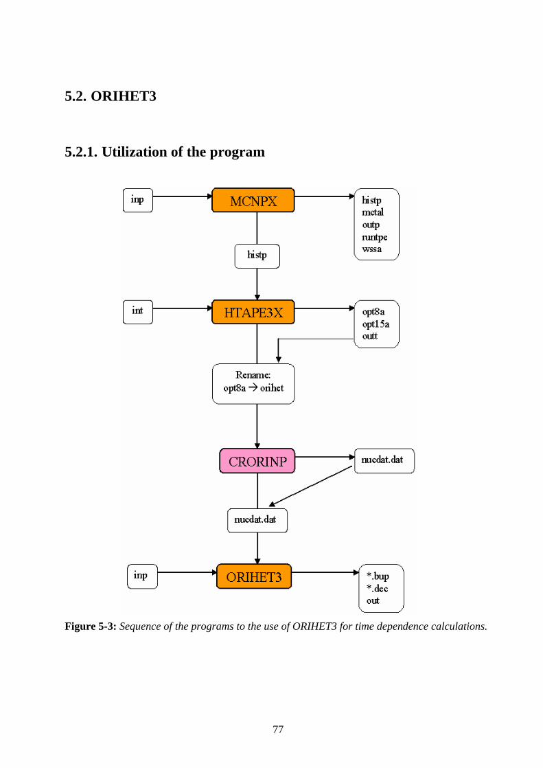
77
5.2. ORIHET3
5.2.1. Utilization of the program
Figure 5-3: Sequence of the programs to the use of ORIHET3 for time dependence calculations.
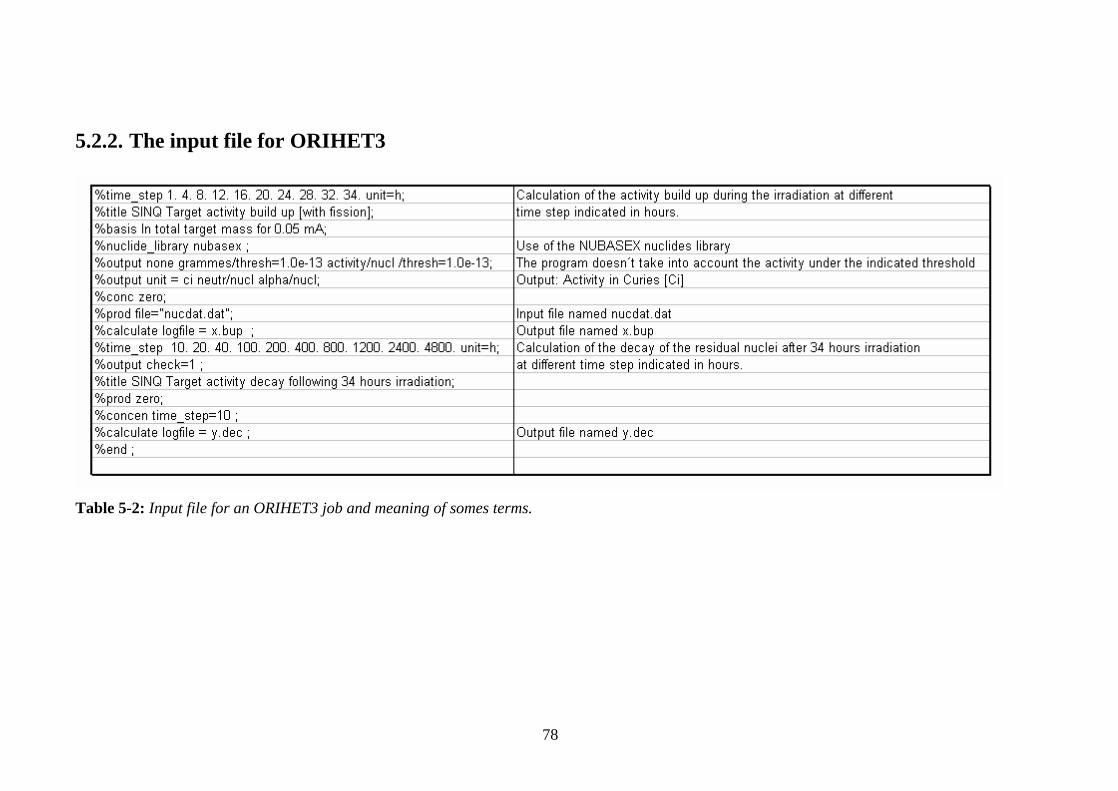
78
5.2.2. The input file for ORIHET3
Table 5-2: Input file for an ORIHET3 job and meaning of somes terms.
79
Conclusion Within the Beta-Testing of MCNPX, investigations to study the Accelerator Driven Systems are performed at the Institut for Reactor Safety (IRS). The first chapters were dedicated to the description of the spallation reaction, to give the charasteristics necessary for a good understanding of the results of this reaction and to the presentation of the models which had been used in this work. The main work of this study was the validation of the implementation of the INCL4+ABLA code in the new beta version 2.5e of MCNPX after the code of the Cugnon group was integrated in MCNPX. First the normalized MCNPX results were compared with the corresponding results obtained with Cugnon Stand-alone and they were in very good agreement for the fission part and for the spallation part too. Particularly, this study shows how to define the input parameters and the corresponding normalization to obtain the spallation yields. An important part was devoted to the detailed understanding of the calculations of the geometrical cross section. The MCNPX results were compared with the experimental data at different energy level. At 1 GeV proton energy, MCNPX results with recommended input parameters were in good agreement with the data from the GSI (Darmstadt) and the data from ISTC (Moscow). A dispersion of the raw data from ISTC was found at 600 MeV proton energy. The data from GSI for 500 MeV were in very good agreement for the spallation part, but a difference of 40% was observed for the fission part which would be disappear after the discussed correction of the experimental data. After the validation of MCNPX, we investigated to the LiSoR experiment. This experiment has the role to prepare the MEGAPIE project by simulating the MEGAPIE conditions (under irradiation, under strain and in the presence of Lead-Bismuth-Eutectic). We focused this study on predictions for the Polonium generation. Indeed, the Polonium is an important problem of MEGAPIE because it may cause contamination of the target. The main isotopes 208Po and 209Po were particularly considered due to their α-activity. An interesting question is to study the 210Po which is produced by activation and the program ORIHET3 used for the decay calculations doesn’t take into account activation. The last chapter of this work presented two codes for depletion calculation: ORIHET3 developed at PSI and KAPROS developed at FZK. Their characteristics and their uses were explained. The next step is the comparison of calculations to evaluate the two codes and especially to study the 210Po generation by activation.
80
Annex A Distribution of spallation yields before normalization calculated by MCNPX and obtained by HTAPE3X and with the tally 8 option These results are performed with the INCL4+ABLA model for 300.000 cascades histories by irradiation of a 208Pb target by 1 GeV proton beam. The LCA input card is the one defined in section 3.1. The first table is the result from HTAPE3X. This is the direct output file opt8a except the column with the mass number A. Indeed, it is easier to have the same value in order to compare with the output file obtained with tally 8. The data are given only for the spallation corresponding to charge munber ranging between 65 and 85.
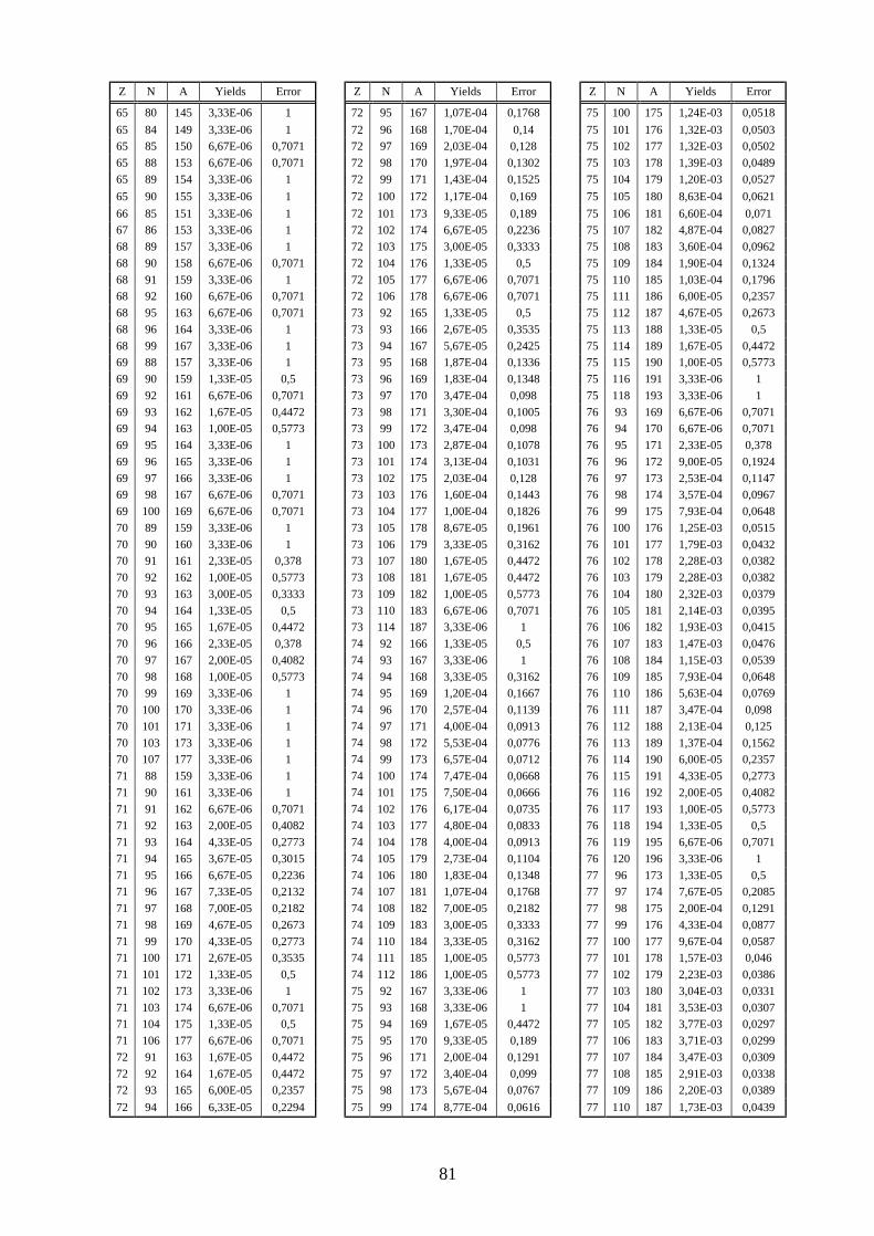
81
Z N A Yields Error Z N A Yields Error Z N A Yields Error
65 80 145 3,33E-06 1 72 95 167 1,07E-04 0,1768 75 100 175 1,24E-03 0,0518 65 84 149 3,33E-06 1 72 96 168 1,70E-04 0,14 75 101 176 1,32E-03 0,0503 65 85 150 6,67E-06 0,7071 72 97 169 2,03E-04 0,128 75 102 177 1,32E-03 0,0502 65 88 153 6,67E-06 0,7071 72 98 170 1,97E-04 0,1302 75 103 178 1,39E-03 0,0489 65 89 154 3,33E-06 1 72 99 171 1,43E-04 0,1525 75 104 179 1,20E-03 0,0527 65 90 155 3,33E-06 1 72 100 172 1,17E-04 0,169 75 105 180 8,63E-04 0,0621 66 85 151 3,33E-06 1 72 101 173 9,33E-05 0,189 75 106 181 6,60E-04 0,071 67 86 153 3,33E-06 1 72 102 174 6,67E-05 0,2236 75 107 182 4,87E-04 0,0827 68 89 157 3,33E-06 1 72 103 175 3,00E-05 0,3333 75 108 183 3,60E-04 0,0962 68 90 158 6,67E-06 0,7071 72 104 176 1,33E-05 0,5 75 109 184 1,90E-04 0,1324 68 91 159 3,33E-06 1 72 105 177 6,67E-06 0,7071 75 110 185 1,03E-04 0,1796 68 92 160 6,67E-06 0,7071 72 106 178 6,67E-06 0,7071 75 111 186 6,00E-05 0,2357 68 95 163 6,67E-06 0,7071 73 92 165 1,33E-05 0,5 75 112 187 4,67E-05 0,2673 68 96 164 3,33E-06 1 73 93 166 2,67E-05 0,3535 75 113 188 1,33E-05 0,5 68 99 167 3,33E-06 1 73 94 167 5,67E-05 0,2425 75 114 189 1,67E-05 0,4472 69 88 157 3,33E-06 1 73 95 168 1,87E-04 0,1336 75 115 190 1,00E-05 0,5773 69 90 159 1,33E-05 0,5 73 96 169 1,83E-04 0,1348 75 116 191 3,33E-06 1 69 92 161 6,67E-06 0,7071 73 97 170 3,47E-04 0,098 75 118 193 3,33E-06 1 69 93 162 1,67E-05 0,4472 73 98 171 3,30E-04 0,1005 76 93 169 6,67E-06 0,7071 69 94 163 1,00E-05 0,5773 73 99 172 3,47E-04 0,098 76 94 170 6,67E-06 0,7071 69 95 164 3,33E-06 1 73 100 173 2,87E-04 0,1078 76 95 171 2,33E-05 0,378 69 96 165 3,33E-06 1 73 101 174 3,13E-04 0,1031 76 96 172 9,00E-05 0,1924 69 97 166 3,33E-06 1 73 102 175 2,03E-04 0,128 76 97 173 2,53E-04 0,1147 69 98 167 6,67E-06 0,7071 73 103 176 1,60E-04 0,1443 76 98 174 3,57E-04 0,0967 69 100 169 6,67E-06 0,7071 73 104 177 1,00E-04 0,1826 76 99 175 7,93E-04 0,0648 70 89 159 3,33E-06 1 73 105 178 8,67E-05 0,1961 76 100 176 1,25E-03 0,0515 70 90 160 3,33E-06 1 73 106 179 3,33E-05 0,3162 76 101 177 1,79E-03 0,0432 70 91 161 2,33E-05 0,378 73 107 180 1,67E-05 0,4472 76 102 178 2,28E-03 0,0382 70 92 162 1,00E-05 0,5773 73 108 181 1,67E-05 0,4472 76 103 179 2,28E-03 0,0382 70 93 163 3,00E-05 0,3333 73 109 182 1,00E-05 0,5773 76 104 180 2,32E-03 0,0379 70 94 164 1,33E-05 0,5 73 110 183 6,67E-06 0,7071 76 105 181 2,14E-03 0,0395 70 95 165 1,67E-05 0,4472 73 114 187 3,33E-06 1 76 106 182 1,93E-03 0,0415 70 96 166 2,33E-05 0,378 74 92 166 1,33E-05 0,5 76 107 183 1,47E-03 0,0476 70 97 167 2,00E-05 0,4082 74 93 167 3,33E-06 1 76 108 184 1,15E-03 0,0539 70 98 168 1,00E-05 0,5773 74 94 168 3,33E-05 0,3162 76 109 185 7,93E-04 0,0648 70 99 169 3,33E-06 1 74 95 169 1,20E-04 0,1667 76 110 186 5,63E-04 0,0769 70 100 170 3,33E-06 1 74 96 170 2,57E-04 0,1139 76 111 187 3,47E-04 0,098 70 101 171 3,33E-06 1 74 97 171 4,00E-04 0,0913 76 112 188 2,13E-04 0,125 70 103 173 3,33E-06 1 74 98 172 5,53E-04 0,0776 76 113 189 1,37E-04 0,1562 70 107 177 3,33E-06 1 74 99 173 6,57E-04 0,0712 76 114 190 6,00E-05 0,2357 71 88 159 3,33E-06 1 74 100 174 7,47E-04 0,0668 76 115 191 4,33E-05 0,2773 71 90 161 3,33E-06 1 74 101 175 7,50E-04 0,0666 76 116 192 2,00E-05 0,4082 71 91 162 6,67E-06 0,7071 74 102 176 6,17E-04 0,0735 76 117 193 1,00E-05 0,5773 71 92 163 2,00E-05 0,4082 74 103 177 4,80E-04 0,0833 76 118 194 1,33E-05 0,5 71 93 164 4,33E-05 0,2773 74 104 178 4,00E-04 0,0913 76 119 195 6,67E-06 0,7071 71 94 165 3,67E-05 0,3015 74 105 179 2,73E-04 0,1104 76 120 196 3,33E-06 1 71 95 166 6,67E-05 0,2236 74 106 180 1,83E-04 0,1348 77 96 173 1,33E-05 0,5 71 96 167 7,33E-05 0,2132 74 107 181 1,07E-04 0,1768 77 97 174 7,67E-05 0,2085 71 97 168 7,00E-05 0,2182 74 108 182 7,00E-05 0,2182 77 98 175 2,00E-04 0,1291 71 98 169 4,67E-05 0,2673 74 109 183 3,00E-05 0,3333 77 99 176 4,33E-04 0,0877 71 99 170 4,33E-05 0,2773 74 110 184 3,33E-05 0,3162 77 100 177 9,67E-04 0,0587 71 100 171 2,67E-05 0,3535 74 111 185 1,00E-05 0,5773 77 101 178 1,57E-03 0,046 71 101 172 1,33E-05 0,5 74 112 186 1,00E-05 0,5773 77 102 179 2,23E-03 0,0386 71 102 173 3,33E-06 1 75 92 167 3,33E-06 1 77 103 180 3,04E-03 0,0331 71 103 174 6,67E-06 0,7071 75 93 168 3,33E-06 1 77 104 181 3,53E-03 0,0307 71 104 175 1,33E-05 0,5 75 94 169 1,67E-05 0,4472 77 105 182 3,77E-03 0,0297 71 106 177 6,67E-06 0,7071 75 95 170 9,33E-05 0,189 77 106 183 3,71E-03 0,0299 72 91 163 1,67E-05 0,4472 75 96 171 2,00E-04 0,1291 77 107 184 3,47E-03 0,0309 72 92 164 1,67E-05 0,4472 75 97 172 3,40E-04 0,099 77 108 185 2,91E-03 0,0338 72 93 165 6,00E-05 0,2357 75 98 173 5,67E-04 0,0767 77 109 186 2,20E-03 0,0389 72 94 166 6,33E-05 0,2294 75 99 174 8,77E-04 0,0616 77 110 187 1,73E-03 0,0439
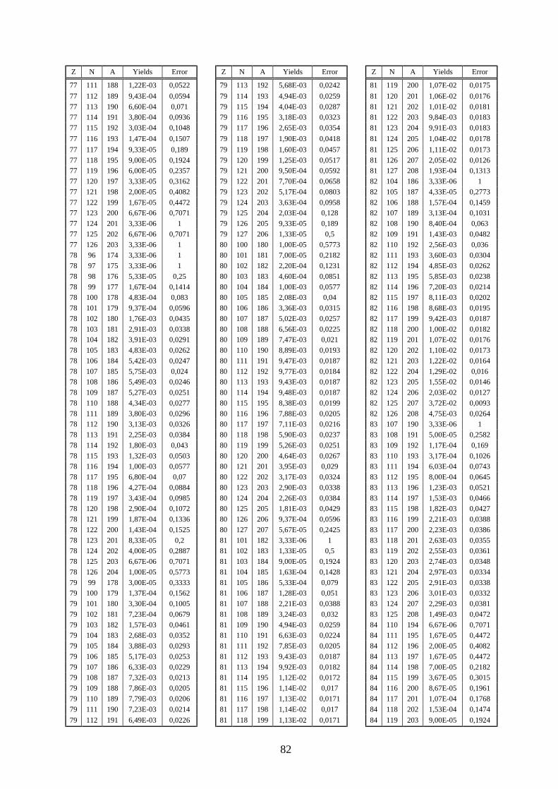
82
Z N A Yields Error Z N A Yields Error Z N A Yields Error
77 111 188 1,22E-03 0,0522 79 113 192 5,68E-03 0,0242 81 119 200 1,07E-02 0,0175 77 112 189 9,43E-04 0,0594 79 114 193 4,94E-03 0,0259 81 120 201 1,06E-02 0,0176 77 113 190 6,60E-04 0,071 79 115 194 4,04E-03 0,0287 81 121 202 1,01E-02 0,0181 77 114 191 3,80E-04 0,0936 79 116 195 3,18E-03 0,0323 81 122 203 9,84E-03 0,0183 77 115 192 3,03E-04 0,1048 79 117 196 2,65E-03 0,0354 81 123 204 9,91E-03 0,0183 77 116 193 1,47E-04 0,1507 79 118 197 1,90E-03 0,0418 81 124 205 1,04E-02 0,0178 77 117 194 9,33E-05 0,189 79 119 198 1,60E-03 0,0457 81 125 206 1,11E-02 0,0173 77 118 195 9,00E-05 0,1924 79 120 199 1,25E-03 0,0517 81 126 207 2,05E-02 0,0126 77 119 196 6,00E-05 0,2357 79 121 200 9,50E-04 0,0592 81 127 208 1,93E-04 0,1313 77 120 197 3,33E-05 0,3162 79 122 201 7,70E-04 0,0658 82 104 186 3,33E-06 1 77 121 198 2,00E-05 0,4082 79 123 202 5,17E-04 0,0803 82 105 187 4,33E-05 0,2773 77 122 199 1,67E-05 0,4472 79 124 203 3,63E-04 0,0958 82 106 188 1,57E-04 0,1459 77 123 200 6,67E-06 0,7071 79 125 204 2,03E-04 0,128 82 107 189 3,13E-04 0,1031 77 124 201 3,33E-06 1 79 126 205 9,33E-05 0,189 82 108 190 8,40E-04 0,063 77 125 202 6,67E-06 0,7071 79 127 206 1,33E-05 0,5 82 109 191 1,43E-03 0,0482 77 126 203 3,33E-06 1 80 100 180 1,00E-05 0,5773 82 110 192 2,56E-03 0,036 78 96 174 3,33E-06 1 80 101 181 7,00E-05 0,2182 82 111 193 3,60E-03 0,0304 78 97 175 3,33E-06 1 80 102 182 2,20E-04 0,1231 82 112 194 4,85E-03 0,0262 78 98 176 5,33E-05 0,25 80 103 183 4,60E-04 0,0851 82 113 195 5,85E-03 0,0238 78 99 177 1,67E-04 0,1414 80 104 184 1,00E-03 0,0577 82 114 196 7,20E-03 0,0214 78 100 178 4,83E-04 0,083 80 105 185 2,08E-03 0,04 82 115 197 8,11E-03 0,0202 78 101 179 9,37E-04 0,0596 80 106 186 3,36E-03 0,0315 82 116 198 8,68E-03 0,0195 78 102 180 1,76E-03 0,0435 80 107 187 5,02E-03 0,0257 82 117 199 9,42E-03 0,0187 78 103 181 2,91E-03 0,0338 80 108 188 6,56E-03 0,0225 82 118 200 1,00E-02 0,0182 78 104 182 3,91E-03 0,0291 80 109 189 7,47E-03 0,021 82 119 201 1,07E-02 0,0176 78 105 183 4,83E-03 0,0262 80 110 190 8,89E-03 0,0193 82 120 202 1,10E-02 0,0173 78 106 184 5,42E-03 0,0247 80 111 191 9,47E-03 0,0187 82 121 203 1,22E-02 0,0164 78 107 185 5,75E-03 0,024 80 112 192 9,77E-03 0,0184 82 122 204 1,29E-02 0,016 78 108 186 5,49E-03 0,0246 80 113 193 9,43E-03 0,0187 82 123 205 1,55E-02 0,0146 78 109 187 5,27E-03 0,0251 80 114 194 9,48E-03 0,0187 82 124 206 2,03E-02 0,0127 78 110 188 4,34E-03 0,0277 80 115 195 8,38E-03 0,0199 82 125 207 3,72E-02 0,0093 78 111 189 3,80E-03 0,0296 80 116 196 7,88E-03 0,0205 82 126 208 4,75E-03 0,0264 78 112 190 3,13E-03 0,0326 80 117 197 7,11E-03 0,0216 83 107 190 3,33E-06 1 78 113 191 2,25E-03 0,0384 80 118 198 5,90E-03 0,0237 83 108 191 5,00E-05 0,2582 78 114 192 1,80E-03 0,043 80 119 199 5,26E-03 0,0251 83 109 192 1,17E-04 0,169 78 115 193 1,32E-03 0,0503 80 120 200 4,64E-03 0,0267 83 110 193 3,17E-04 0,1026 78 116 194 1,00E-03 0,0577 80 121 201 3,95E-03 0,029 83 111 194 6,03E-04 0,0743 78 117 195 6,80E-04 0,07 80 122 202 3,17E-03 0,0324 83 112 195 8,00E-04 0,0645 78 118 196 4,27E-04 0,0884 80 123 203 2,90E-03 0,0338 83 113 196 1,23E-03 0,0521 78 119 197 3,43E-04 0,0985 80 124 204 2,26E-03 0,0384 83 114 197 1,53E-03 0,0466 78 120 198 2,90E-04 0,1072 80 125 205 1,81E-03 0,0429 83 115 198 1,82E-03 0,0427 78 121 199 1,87E-04 0,1336 80 126 206 9,37E-04 0,0596 83 116 199 2,21E-03 0,0388 78 122 200 1,43E-04 0,1525 80 127 207 5,67E-05 0,2425 83 117 200 2,23E-03 0,0386 78 123 201 8,33E-05 0,2 81 101 182 3,33E-06 1 83 118 201 2,63E-03 0,0355 78 124 202 4,00E-05 0,2887 81 102 183 1,33E-05 0,5 83 119 202 2,55E-03 0,0361 78 125 203 6,67E-06 0,7071 81 103 184 9,00E-05 0,1924 83 120 203 2,74E-03 0,0348 78 126 204 1,00E-05 0,5773 81 104 185 1,63E-04 0,1428 83 121 204 2,97E-03 0,0334 79 99 178 3,00E-05 0,3333 81 105 186 5,33E-04 0,079 83 122 205 2,91E-03 0,0338 79 100 179 1,37E-04 0,1562 81 106 187 1,28E-03 0,051 83 123 206 3,01E-03 0,0332 79 101 180 3,30E-04 0,1005 81 107 188 2,21E-03 0,0388 83 124 207 2,29E-03 0,0381 79 102 181 7,23E-04 0,0679 81 108 189 3,24E-03 0,032 83 125 208 1,49E-03 0,0472 79 103 182 1,57E-03 0,0461 81 109 190 4,94E-03 0,0259 84 110 194 6,67E-06 0,7071 79 104 183 2,68E-03 0,0352 81 110 191 6,63E-03 0,0224 84 111 195 1,67E-05 0,4472 79 105 184 3,88E-03 0,0293 81 111 192 7,85E-03 0,0205 84 112 196 2,00E-05 0,4082 79 106 185 5,17E-03 0,0253 81 112 193 9,43E-03 0,0187 84 113 197 1,67E-05 0,4472 79 107 186 6,33E-03 0,0229 81 113 194 9,92E-03 0,0182 84 114 198 7,00E-05 0,2182 79 108 187 7,32E-03 0,0213 81 114 195 1,12E-02 0,0172 84 115 199 3,67E-05 0,3015 79 109 188 7,86E-03 0,0205 81 115 196 1,14E-02 0,017 84 116 200 8,67E-05 0,1961 79 110 189 7,79E-03 0,0206 81 116 197 1,13E-02 0,0171 84 117 201 1,07E-04 0,1768 79 111 190 7,23E-03 0,0214 81 117 198 1,14E-02 0,017 84 118 202 1,53E-04 0,1474 79 112 191 6,49E-03 0,0226 81 118 199 1,13E-02 0,0171 84 119 203 9,00E-05 0,1924

83
Z N A Yields Error
84 120 204 9,00E-05 0,1924 84 121 205 7,00E-05 0,2182 84 122 206 6,00E-05 0,2357 84 123 207 3,00E-05 0,3333 84 124 208 3,33E-06 1 85 120 205 3,33E-06 1
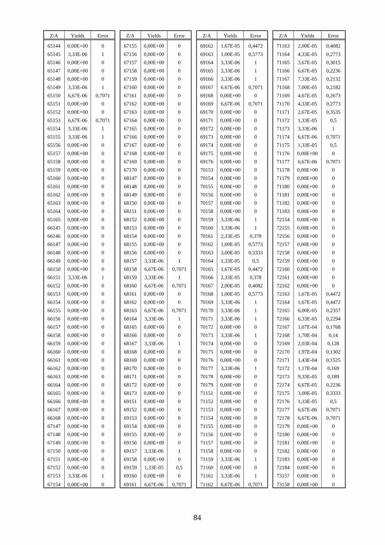
84
Z/A Yields Error Z/A Yields Error Z/A Yields Error Z/A Yields Error
65144 0,00E+00 0 67155 0,00E+00 0 69162 1,67E-05 0,4472 71163 2,00E-05 0,4082 65145 3,33E-06 1 67156 0,00E+00 0 69163 1,00E-05 0,5773 71164 4,33E-05 0,2773 65146 0,00E+00 0 67157 0,00E+00 0 69164 3,33E-06 1 71165 3,67E-05 0,3015 65147 0,00E+00 0 67158 0,00E+00 0 69165 3,33E-06 1 71166 6,67E-05 0,2236 65148 0,00E+00 0 67159 0,00E+00 0 69166 3,33E-06 1 71167 7,33E-05 0,2132 65149 3,33E-06 1 67160 0,00E+00 0 69167 6,67E-06 0,7071 71168 7,00E-05 0,2182 65150 6,67E-06 0,7071 67161 0,00E+00 0 69168 0,00E+00 0 71169 4,67E-05 0,2673 65151 0,00E+00 0 67162 0,00E+00 0 69169 6,67E-06 0,7071 71170 4,33E-05 0,2773 65152 0,00E+00 0 67163 0,00E+00 0 69170 0,00E+00 0 71171 2,67E-05 0,3535 65153 6,67E-06 0,7071 67164 0,00E+00 0 69171 0,00E+00 0 71172 1,33E-05 0,5 65154 3,33E-06 1 67165 0,00E+00 0 69172 0,00E+00 0 71173 3,33E-06 1 65155 3,33E-06 1 67166 0,00E+00 0 69173 0,00E+00 0 71174 6,67E-06 0,7071 65156 0,00E+00 0 67167 0,00E+00 0 69174 0,00E+00 0 71175 1,33E-05 0,5 65157 0,00E+00 0 67168 0,00E+00 0 69175 0,00E+00 0 71176 0,00E+00 0 65158 0,00E+00 0 67169 0,00E+00 0 69176 0,00E+00 0 71177 6,67E-06 0,7071 65159 0,00E+00 0 67170 0,00E+00 0 70153 0,00E+00 0 71178 0,00E+00 0 65160 0,00E+00 0 68147 0,00E+00 0 70154 0,00E+00 0 71179 0,00E+00 0 65161 0,00E+00 0 68148 0,00E+00 0 70155 0,00E+00 0 71180 0,00E+00 0 65162 0,00E+00 0 68149 0,00E+00 0 70156 0,00E+00 0 71181 0,00E+00 0 65163 0,00E+00 0 68150 0,00E+00 0 70157 0,00E+00 0 71182 0,00E+00 0 65164 0,00E+00 0 68151 0,00E+00 0 70158 0,00E+00 0 71183 0,00E+00 0 65165 0,00E+00 0 68152 0,00E+00 0 70159 3,33E-06 1 72154 0,00E+00 0 66145 0,00E+00 0 68153 0,00E+00 0 70160 3,33E-06 1 72155 0,00E+00 0 66146 0,00E+00 0 68154 0,00E+00 0 70161 2,33E-05 0,378 72156 0,00E+00 0 66147 0,00E+00 0 68155 0,00E+00 0 70162 1,00E-05 0,5773 72157 0,00E+00 0 66148 0,00E+00 0 68156 0,00E+00 0 70163 3,00E-05 0,3333 72158 0,00E+00 0 66149 0,00E+00 0 68157 3,33E-06 1 70164 1,33E-05 0,5 72159 0,00E+00 0 66150 0,00E+00 0 68158 6,67E-06 0,7071 70165 1,67E-05 0,4472 72160 0,00E+00 0 66151 3,33E-06 1 68159 3,33E-06 1 70166 2,33E-05 0,378 72161 0,00E+00 0 66152 0,00E+00 0 68160 6,67E-06 0,7071 70167 2,00E-05 0,4082 72162 0,00E+00 0 66153 0,00E+00 0 68161 0,00E+00 0 70168 1,00E-05 0,5773 72163 1,67E-05 0,4472 66154 0,00E+00 0 68162 0,00E+00 0 70169 3,33E-06 1 72164 1,67E-05 0,4472 66155 0,00E+00 0 68163 6,67E-06 0,7071 70170 3,33E-06 1 72165 6,00E-05 0,2357 66156 0,00E+00 0 68164 3,33E-06 1 70171 3,33E-06 1 72166 6,33E-05 0,2294 66157 0,00E+00 0 68165 0,00E+00 0 70172 0,00E+00 0 72167 1,07E-04 0,1768 66158 0,00E+00 0 68166 0,00E+00 0 70173 3,33E-06 1 72168 1,70E-04 0,14 66159 0,00E+00 0 68167 3,33E-06 1 70174 0,00E+00 0 72169 2,03E-04 0,128 66160 0,00E+00 0 68168 0,00E+00 0 70175 0,00E+00 0 72170 1,97E-04 0,1302 66161 0,00E+00 0 68169 0,00E+00 0 70176 0,00E+00 0 72171 1,43E-04 0,1525 66162 0,00E+00 0 68170 0,00E+00 0 70177 3,33E-06 1 72172 1,17E-04 0,169 66163 0,00E+00 0 68171 0,00E+00 0 70178 0,00E+00 0 72173 9,33E-05 0,189 66164 0,00E+00 0 68172 0,00E+00 0 70179 0,00E+00 0 72174 6,67E-05 0,2236 66165 0,00E+00 0 68173 0,00E+00 0 71151 0,00E+00 0 72175 3,00E-05 0,3333 66166 0,00E+00 0 69151 0,00E+00 0 71152 0,00E+00 0 72176 1,33E-05 0,5 66167 0,00E+00 0 69152 0,00E+00 0 71153 0,00E+00 0 72177 6,67E-06 0,7071 66168 0,00E+00 0 69153 0,00E+00 0 71154 0,00E+00 0 72178 6,67E-06 0,7071 67147 0,00E+00 0 69154 0,00E+00 0 71155 0,00E+00 0 72179 0,00E+00 0 67148 0,00E+00 0 69155 0,00E+00 0 71156 0,00E+00 0 72180 0,00E+00 0 67149 0,00E+00 0 69156 0,00E+00 0 71157 0,00E+00 0 72181 0,00E+00 0 67150 0,00E+00 0 69157 3,33E-06 1 71158 0,00E+00 0 72182 0,00E+00 0 67151 0,00E+00 0 69158 0,00E+00 0 71159 3,33E-06 1 72183 0,00E+00 0 67152 0,00E+00 0 69159 1,33E-05 0,5 71160 0,00E+00 0 72184 0,00E+00 0 67153 3,33E-06 1 69160 0,00E+00 0 71161 3,33E-06 1 73157 0,00E+00 0
67154 0,00E+00 0 69161 6,67E-06 0,7071 71162 6,67E-06 0,7071 73158 0,00E+00 0
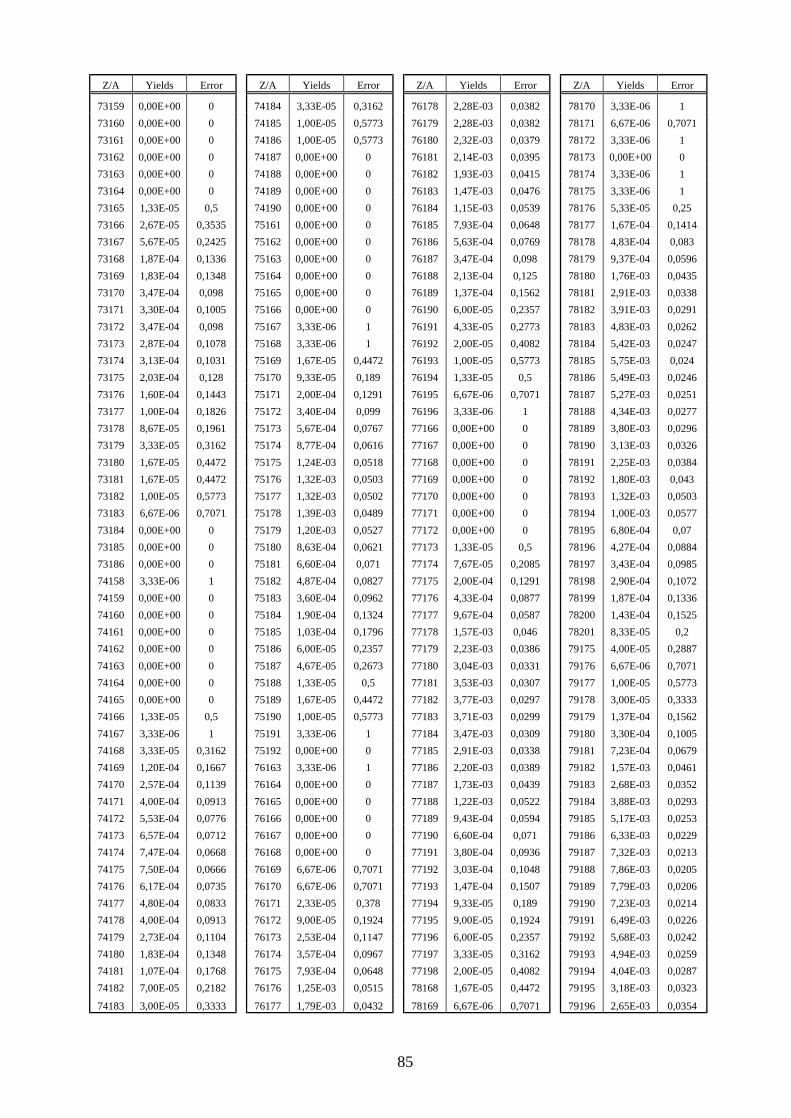
85
Z/A Yields Error Z/A Yields Error Z/A Yields Error Z/A Yields Error
73159 0,00E+00 0 74184 3,33E-05 0,3162 76178 2,28E-03 0,0382 78170 3,33E-06 1 73160 0,00E+00 0 74185 1,00E-05 0,5773 76179 2,28E-03 0,0382 78171 6,67E-06 0,7071 73161 0,00E+00 0 74186 1,00E-05 0,5773 76180 2,32E-03 0,0379 78172 3,33E-06 1 73162 0,00E+00 0 74187 0,00E+00 0 76181 2,14E-03 0,0395 78173 0,00E+00 0 73163 0,00E+00 0 74188 0,00E+00 0 76182 1,93E-03 0,0415 78174 3,33E-06 1 73164 0,00E+00 0 74189 0,00E+00 0 76183 1,47E-03 0,0476 78175 3,33E-06 1 73165 1,33E-05 0,5 74190 0,00E+00 0 76184 1,15E-03 0,0539 78176 5,33E-05 0,25 73166 2,67E-05 0,3535 75161 0,00E+00 0 76185 7,93E-04 0,0648 78177 1,67E-04 0,1414 73167 5,67E-05 0,2425 75162 0,00E+00 0 76186 5,63E-04 0,0769 78178 4,83E-04 0,083 73168 1,87E-04 0,1336 75163 0,00E+00 0 76187 3,47E-04 0,098 78179 9,37E-04 0,0596 73169 1,83E-04 0,1348 75164 0,00E+00 0 76188 2,13E-04 0,125 78180 1,76E-03 0,0435 73170 3,47E-04 0,098 75165 0,00E+00 0 76189 1,37E-04 0,1562 78181 2,91E-03 0,0338 73171 3,30E-04 0,1005 75166 0,00E+00 0 76190 6,00E-05 0,2357 78182 3,91E-03 0,0291 73172 3,47E-04 0,098 75167 3,33E-06 1 76191 4,33E-05 0,2773 78183 4,83E-03 0,0262 73173 2,87E-04 0,1078 75168 3,33E-06 1 76192 2,00E-05 0,4082 78184 5,42E-03 0,0247 73174 3,13E-04 0,1031 75169 1,67E-05 0,4472 76193 1,00E-05 0,5773 78185 5,75E-03 0,024 73175 2,03E-04 0,128 75170 9,33E-05 0,189 76194 1,33E-05 0,5 78186 5,49E-03 0,0246 73176 1,60E-04 0,1443 75171 2,00E-04 0,1291 76195 6,67E-06 0,7071 78187 5,27E-03 0,0251 73177 1,00E-04 0,1826 75172 3,40E-04 0,099 76196 3,33E-06 1 78188 4,34E-03 0,0277 73178 8,67E-05 0,1961 75173 5,67E-04 0,0767 77166 0,00E+00 0 78189 3,80E-03 0,0296 73179 3,33E-05 0,3162 75174 8,77E-04 0,0616 77167 0,00E+00 0 78190 3,13E-03 0,0326 73180 1,67E-05 0,4472 75175 1,24E-03 0,0518 77168 0,00E+00 0 78191 2,25E-03 0,0384 73181 1,67E-05 0,4472 75176 1,32E-03 0,0503 77169 0,00E+00 0 78192 1,80E-03 0,043 73182 1,00E-05 0,5773 75177 1,32E-03 0,0502 77170 0,00E+00 0 78193 1,32E-03 0,0503 73183 6,67E-06 0,7071 75178 1,39E-03 0,0489 77171 0,00E+00 0 78194 1,00E-03 0,0577 73184 0,00E+00 0 75179 1,20E-03 0,0527 77172 0,00E+00 0 78195 6,80E-04 0,07 73185 0,00E+00 0 75180 8,63E-04 0,0621 77173 1,33E-05 0,5 78196 4,27E-04 0,0884 73186 0,00E+00 0 75181 6,60E-04 0,071 77174 7,67E-05 0,2085 78197 3,43E-04 0,0985 74158 3,33E-06 1 75182 4,87E-04 0,0827 77175 2,00E-04 0,1291 78198 2,90E-04 0,1072 74159 0,00E+00 0 75183 3,60E-04 0,0962 77176 4,33E-04 0,0877 78199 1,87E-04 0,1336 74160 0,00E+00 0 75184 1,90E-04 0,1324 77177 9,67E-04 0,0587 78200 1,43E-04 0,1525 74161 0,00E+00 0 75185 1,03E-04 0,1796 77178 1,57E-03 0,046 78201 8,33E-05 0,2 74162 0,00E+00 0 75186 6,00E-05 0,2357 77179 2,23E-03 0,0386 79175 4,00E-05 0,2887 74163 0,00E+00 0 75187 4,67E-05 0,2673 77180 3,04E-03 0,0331 79176 6,67E-06 0,7071 74164 0,00E+00 0 75188 1,33E-05 0,5 77181 3,53E-03 0,0307 79177 1,00E-05 0,5773 74165 0,00E+00 0 75189 1,67E-05 0,4472 77182 3,77E-03 0,0297 79178 3,00E-05 0,3333 74166 1,33E-05 0,5 75190 1,00E-05 0,5773 77183 3,71E-03 0,0299 79179 1,37E-04 0,1562 74167 3,33E-06 1 75191 3,33E-06 1 77184 3,47E-03 0,0309 79180 3,30E-04 0,1005 74168 3,33E-05 0,3162 75192 0,00E+00 0 77185 2,91E-03 0,0338 79181 7,23E-04 0,0679 74169 1,20E-04 0,1667 76163 3,33E-06 1 77186 2,20E-03 0,0389 79182 1,57E-03 0,0461 74170 2,57E-04 0,1139 76164 0,00E+00 0 77187 1,73E-03 0,0439 79183 2,68E-03 0,0352 74171 4,00E-04 0,0913 76165 0,00E+00 0 77188 1,22E-03 0,0522 79184 3,88E-03 0,0293 74172 5,53E-04 0,0776 76166 0,00E+00 0 77189 9,43E-04 0,0594 79185 5,17E-03 0,0253 74173 6,57E-04 0,0712 76167 0,00E+00 0 77190 6,60E-04 0,071 79186 6,33E-03 0,0229 74174 7,47E-04 0,0668 76168 0,00E+00 0 77191 3,80E-04 0,0936 79187 7,32E-03 0,0213 74175 7,50E-04 0,0666 76169 6,67E-06 0,7071 77192 3,03E-04 0,1048 79188 7,86E-03 0,0205 74176 6,17E-04 0,0735 76170 6,67E-06 0,7071 77193 1,47E-04 0,1507 79189 7,79E-03 0,0206 74177 4,80E-04 0,0833 76171 2,33E-05 0,378 77194 9,33E-05 0,189 79190 7,23E-03 0,0214 74178 4,00E-04 0,0913 76172 9,00E-05 0,1924 77195 9,00E-05 0,1924 79191 6,49E-03 0,0226 74179 2,73E-04 0,1104 76173 2,53E-04 0,1147 77196 6,00E-05 0,2357 79192 5,68E-03 0,0242 74180 1,83E-04 0,1348 76174 3,57E-04 0,0967 77197 3,33E-05 0,3162 79193 4,94E-03 0,0259 74181 1,07E-04 0,1768 76175 7,93E-04 0,0648 77198 2,00E-05 0,4082 79194 4,04E-03 0,0287 74182 7,00E-05 0,2182 76176 1,25E-03 0,0515 78168 1,67E-05 0,4472 79195 3,18E-03 0,0323
74183 3,00E-05 0,3333 76177 1,79E-03 0,0432 78169 6,67E-06 0,7071 79196 2,65E-03 0,0354
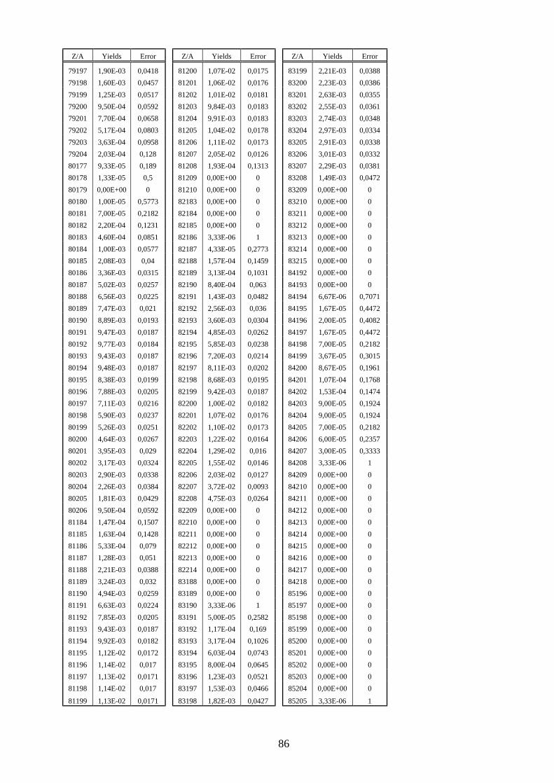
86
Z/A Yields Error Z/A Yields Error Z/A Yields Error
79197 1,90E-03 0,0418 81200 1,07E-02 0,0175 83199 2,21E-03 0,0388 79198 1,60E-03 0,0457 81201 1,06E-02 0,0176 83200 2,23E-03 0,0386 79199 1,25E-03 0,0517 81202 1,01E-02 0,0181 83201 2,63E-03 0,0355 79200 9,50E-04 0,0592 81203 9,84E-03 0,0183 83202 2,55E-03 0,0361 79201 7,70E-04 0,0658 81204 9,91E-03 0,0183 83203 2,74E-03 0,0348 79202 5,17E-04 0,0803 81205 1,04E-02 0,0178 83204 2,97E-03 0,0334 79203 3,63E-04 0,0958 81206 1,11E-02 0,0173 83205 2,91E-03 0,0338 79204 2,03E-04 0,128 81207 2,05E-02 0,0126 83206 3,01E-03 0,0332 80177 9,33E-05 0,189 81208 1,93E-04 0,1313 83207 2,29E-03 0,0381 80178 1,33E-05 0,5 81209 0,00E+00 0 83208 1,49E-03 0,0472 80179 0,00E+00 0 81210 0,00E+00 0 83209 0,00E+00 0 80180 1,00E-05 0,5773 82183 0,00E+00 0 83210 0,00E+00 0 80181 7,00E-05 0,2182 82184 0,00E+00 0 83211 0,00E+00 0 80182 2,20E-04 0,1231 82185 0,00E+00 0 83212 0,00E+00 0 80183 4,60E-04 0,0851 82186 3,33E-06 1 83213 0,00E+00 0 80184 1,00E-03 0,0577 82187 4,33E-05 0,2773 83214 0,00E+00 0 80185 2,08E-03 0,04 82188 1,57E-04 0,1459 83215 0,00E+00 0 80186 3,36E-03 0,0315 82189 3,13E-04 0,1031 84192 0,00E+00 0 80187 5,02E-03 0,0257 82190 8,40E-04 0,063 84193 0,00E+00 0 80188 6,56E-03 0,0225 82191 1,43E-03 0,0482 84194 6,67E-06 0,7071 80189 7,47E-03 0,021 82192 2,56E-03 0,036 84195 1,67E-05 0,4472 80190 8,89E-03 0,0193 82193 3,60E-03 0,0304 84196 2,00E-05 0,4082 80191 9,47E-03 0,0187 82194 4,85E-03 0,0262 84197 1,67E-05 0,4472 80192 9,77E-03 0,0184 82195 5,85E-03 0,0238 84198 7,00E-05 0,2182 80193 9,43E-03 0,0187 82196 7,20E-03 0,0214 84199 3,67E-05 0,3015 80194 9,48E-03 0,0187 82197 8,11E-03 0,0202 84200 8,67E-05 0,1961 80195 8,38E-03 0,0199 82198 8,68E-03 0,0195 84201 1,07E-04 0,1768 80196 7,88E-03 0,0205 82199 9,42E-03 0,0187 84202 1,53E-04 0,1474 80197 7,11E-03 0,0216 82200 1,00E-02 0,0182 84203 9,00E-05 0,1924 80198 5,90E-03 0,0237 82201 1,07E-02 0,0176 84204 9,00E-05 0,1924 80199 5,26E-03 0,0251 82202 1,10E-02 0,0173 84205 7,00E-05 0,2182 80200 4,64E-03 0,0267 82203 1,22E-02 0,0164 84206 6,00E-05 0,2357 80201 3,95E-03 0,029 82204 1,29E-02 0,016 84207 3,00E-05 0,3333 80202 3,17E-03 0,0324 82205 1,55E-02 0,0146 84208 3,33E-06 1 80203 2,90E-03 0,0338 82206 2,03E-02 0,0127 84209 0,00E+00 0 80204 2,26E-03 0,0384 82207 3,72E-02 0,0093 84210 0,00E+00 0 80205 1,81E-03 0,0429 82208 4,75E-03 0,0264 84211 0,00E+00 0 80206 9,50E-04 0,0592 82209 0,00E+00 0 84212 0,00E+00 0 81184 1,47E-04 0,1507 82210 0,00E+00 0 84213 0,00E+00 0 81185 1,63E-04 0,1428 82211 0,00E+00 0 84214 0,00E+00 0 81186 5,33E-04 0,079 82212 0,00E+00 0 84215 0,00E+00 0 81187 1,28E-03 0,051 82213 0,00E+00 0 84216 0,00E+00 0 81188 2,21E-03 0,0388 82214 0,00E+00 0 84217 0,00E+00 0 81189 3,24E-03 0,032 83188 0,00E+00 0 84218 0,00E+00 0 81190 4,94E-03 0,0259 83189 0,00E+00 0 85196 0,00E+00 0 81191 6,63E-03 0,0224 83190 3,33E-06 1 85197 0,00E+00 0 81192 7,85E-03 0,0205 83191 5,00E-05 0,2582 85198 0,00E+00 0 81193 9,43E-03 0,0187 83192 1,17E-04 0,169 85199 0,00E+00 0 81194 9,92E-03 0,0182 83193 3,17E-04 0,1026 85200 0,00E+00 0 81195 1,12E-02 0,0172 83194 6,03E-04 0,0743 85201 0,00E+00 0 81196 1,14E-02 0,017 83195 8,00E-04 0,0645 85202 0,00E+00 0 81197 1,13E-02 0,0171 83196 1,23E-03 0,0521 85203 0,00E+00 0 81198 1,14E-02 0,017 83197 1,53E-03 0,0466 85204 0,00E+00 0
81199 1,13E-02 0,0171 83198 1,82E-03 0,0427 85205 3,33E-06 1
87
Annex B Experimental data at 600 MeV for 208Pb These experimental data are preliminary data from ISTC#2002 [49].
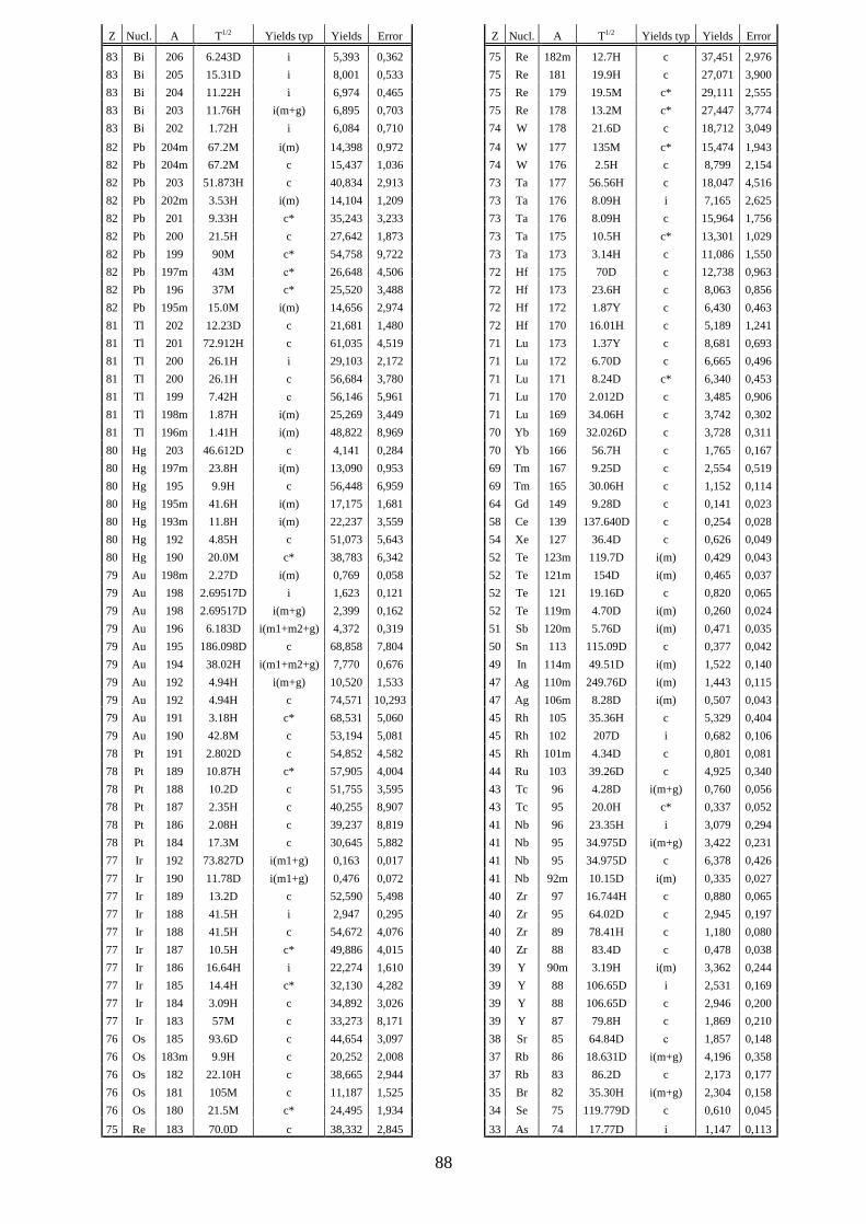
88
Z Nucl. A T1/2 Yields typ Yields Error Z Nucl. A T1/2 Yields typ Yields Error
83 Bi 206 6.243D i 5,393 0,362 75 Re 182m 12.7H c 37,451 2,976 83 Bi 205 15.31D i 8,001 0,533 75 Re 181 19.9H c 27,071 3,900 83 Bi 204 11.22H i 6,974 0,465 75 Re 179 19.5M c* 29,111 2,555 83 Bi 203 11.76H i(m+g) 6,895 0,703 75 Re 178 13.2M c* 27,447 3,774 83 Bi 202 1.72H i 6,084 0,710 74 W 178 21.6D c 18,712 3,049 82 Pb 204m 67.2M i(m) 14,398 0,972 74 W 177 135M c* 15,474 1,943 82 Pb 204m 67.2M c 15,437 1,036 74 W 176 2.5H c 8,799 2,154 82 Pb 203 51.873H c 40,834 2,913 73 Ta 177 56.56H c 18,047 4,516 82 Pb 202m 3.53H i(m) 14,104 1,209 73 Ta 176 8.09H i 7,165 2,625 82 Pb 201 9.33H c* 35,243 3,233 73 Ta 176 8.09H c 15,964 1,756 82 Pb 200 21.5H c 27,642 1,873 73 Ta 175 10.5H c* 13,301 1,029 82 Pb 199 90M c* 54,758 9,722 73 Ta 173 3.14H c 11,086 1,550 82 Pb 197m 43M с* 26,648 4,506 72 Hf 175 70D c 12,738 0,963 82 Pb 196 37M c* 25,520 3,488 72 Hf 173 23.6H c 8,063 0,856 82 Pb 195m 15.0M i(m) 14,656 2,974 72 Hf 172 1.87Y c 6,430 0,463 81 Tl 202 12.23D c 21,681 1,480 72 Hf 170 16.01H c 5,189 1,241 81 Tl 201 72.912H c 61,035 4,519 71 Lu 173 1.37Y c 8,681 0,693 81 Tl 200 26.1H i 29,103 2,172 71 Lu 172 6.70D c 6,665 0,496 81 Tl 200 26.1H c 56,684 3,780 71 Lu 171 8.24D c* 6,340 0,453 81 Tl 199 7.42H с 56,146 5,961 71 Lu 170 2.012D c 3,485 0,906 81 Tl 198m 1.87H i(m) 25,269 3,449 71 Lu 169 34.06H c 3,742 0,302 81 Tl 196m 1.41H i(m) 48,822 8,969 70 Yb 169 32.026D c 3,728 0,311 80 Hg 203 46.612D c 4,141 0,284 70 Yb 166 56.7H c 1,765 0,167 80 Hg 197m 23.8H i(m) 13,090 0,953 69 Tm 167 9.25D c 2,554 0,519 80 Hg 195 9.9H c 56,448 6,959 69 Tm 165 30.06H c 1,152 0,114 80 Hg 195m 41.6H i(m) 17,175 1,681 64 Gd 149 9.28D c 0,141 0,023 80 Hg 193m 11.8H i(m) 22,237 3,559 58 Ce 139 137.640D c 0,254 0,028 80 Hg 192 4.85H c 51,073 5,643 54 Xe 127 36.4D c 0,626 0,049 80 Hg 190 20.0M c* 38,783 6,342 52 Te 123m 119.7D i(m) 0,429 0,043 79 Au 198m 2.27D i(m) 0,769 0,058 52 Te 121m 154D i(m) 0,465 0,037 79 Au 198 2.69517D i 1,623 0,121 52 Te 121 19.16D c 0,820 0,065 79 Au 198 2.69517D i(m+g) 2,399 0,162 52 Te 119m 4.70D i(m) 0,260 0,024 79 Au 196 6.183D i(m1+m2+g) 4,372 0,319 51 Sb 120m 5.76D i(m) 0,471 0,035 79 Au 195 186.098D c 68,858 7,804 50 Sn 113 115.09D c 0,377 0,042 79 Au 194 38.02H i(m1+m2+g) 7,770 0,676 49 In 114m 49.51D i(m) 1,522 0,140 79 Au 192 4.94H i(m+g) 10,520 1,533 47 Ag 110m 249.76D i(m) 1,443 0,115 79 Au 192 4.94H c 74,571 10,293 47 Ag 106m 8.28D i(m) 0,507 0,043 79 Au 191 3.18H c* 68,531 5,060 45 Rh 105 35.36H c 5,329 0,404 79 Au 190 42.8M c 53,194 5,081 45 Rh 102 207D i 0,682 0,106 78 Pt 191 2.802D c 54,852 4,582 45 Rh 101m 4.34D c 0,801 0,081 78 Pt 189 10.87H c* 57,905 4,004 44 Ru 103 39.26D c 4,925 0,340 78 Pt 188 10.2D c 51,755 3,595 43 Tc 96 4.28D i(m+g) 0,760 0,056 78 Pt 187 2.35H c 40,255 8,907 43 Tc 95 20.0H c* 0,337 0,052 78 Pt 186 2.08H c 39,237 8,819 41 Nb 96 23.35H i 3,079 0,294 78 Pt 184 17.3M c 30,645 5,882 41 Nb 95 34.975D i(m+g) 3,422 0,231 77 Ir 192 73.827D i(m1+g) 0,163 0,017 41 Nb 95 34.975D c 6,378 0,426 77 Ir 190 11.78D i(m1+g) 0,476 0,072 41 Nb 92m 10.15D i(m) 0,335 0,027 77 Ir 189 13.2D c 52,590 5,498 40 Zr 97 16.744H c 0,880 0,065 77 Ir 188 41.5H i 2,947 0,295 40 Zr 95 64.02D c 2,945 0,197 77 Ir 188 41.5H c 54,672 4,076 40 Zr 89 78.41H c 1,180 0,080 77 Ir 187 10.5H c* 49,886 4,015 40 Zr 88 83.4D c 0,478 0,038 77 Ir 186 16.64H i 22,274 1,610 39 Y 90m 3.19H i(m) 3,362 0,244 77 Ir 185 14.4H c* 32,130 4,282 39 Y 88 106.65D i 2,531 0,169 77 Ir 184 3.09H c 34,892 3,026 39 Y 88 106.65D c 2,946 0,200 77 Ir 183 57M c 33,273 8,171 39 Y 87 79.8H c 1,869 0,210 76 Os 185 93.6D c 44,654 3,097 38 Sr 85 64.84D с 1,857 0,148 76 Os 183m 9.9H c 20,252 2,008 37 Rb 86 18.631D i(m+g) 4,196 0,358 76 Os 182 22.10H c 38,665 2,944 37 Rb 83 86.2D c 2,173 0,177 76 Os 181 105M c 11,187 1,525 35 Br 82 35.30H i(m+g) 2,304 0,158 76 Os 180 21.5M c* 24,495 1,934 34 Se 75 119.779D c 0,610 0,045 75 Re 183 70.0D c 38,332 2,845 33 As 74 17.77D i 1,147 0,113
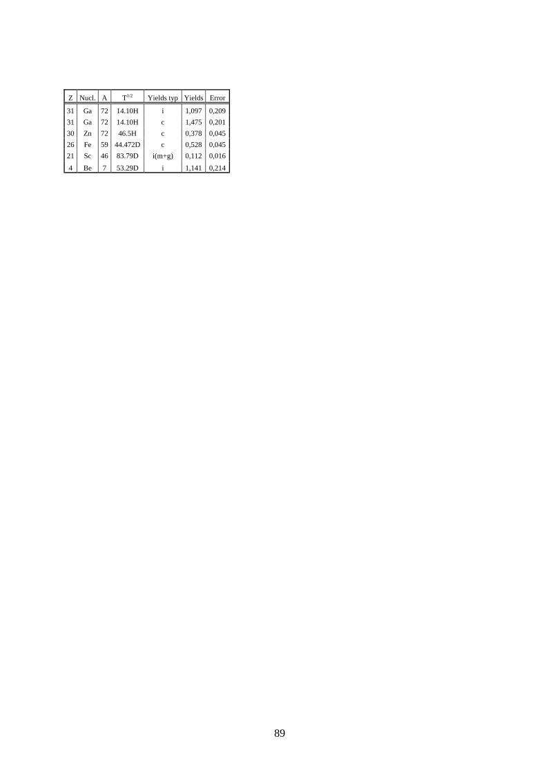
89
Z Nucl. A T1/2 Yields typ Yields Error
31 Ga 72 14.10H i 1,097 0,209 31 Ga 72 14.10H c 1,475 0,201 30 Zn 72 46.5H c 0,378 0,045 26 Fe 59 44.472D c 0,528 0,045 21 Sc 46 83.79D i(m+g) 0,112 0,016 4 Be 7 53.29D i 1,141 0,214
90
Annex C Calculations of volumes of the LiSoR test tube cells
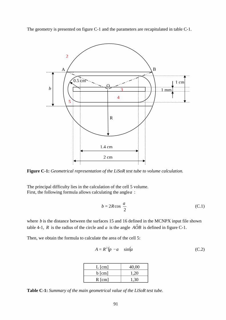
91
The geometry is presented on figure C-1 and the parameters are recapitulated in table C-1.
Figure C-1: Geometrical representation of the LiSoR test tube to volume calculation. The principal difficulty lies in the calculation of the cell 5 volume. First, the following formula allows calculating the angleα :
=
2cos2 αRb (C.1)
where b is the distance between the surfaces 15 and 16 defined in the MCNPX input file shown table 4-1, R is the radius of the circle and α is the angle BOA ˆ is defined in figure C-1. Then, we obtain the formula to calculate the area of the cell 5:
( )( )ααπ sin2 +−= RA (C.2)
L [cm] 40,00 b [cm] 1,20 R [cm] 1,30
Table C-1: Summary of the main geometrical value of the LiSoR test tube.
b 1 mm
1 cm
2 cm
1.4 cm
0.5 cm
A
O
B
R
3
54
2

92
This allows calculating the volumes of the cell 5. The other areas are only rectangles and circles and they represent no difficulties. The results are summarized in table C-2:
cells 1 2 3 4 5
volume [cm3] infinity 112977,12 8 79,42 32,80
Table C-2: Cells volume of the LiSoR test tube geometry.
93
Annex D Concentrations and alpha-activities of Polonium isotopes after 34 hours continuous irradiation in the real geometry target
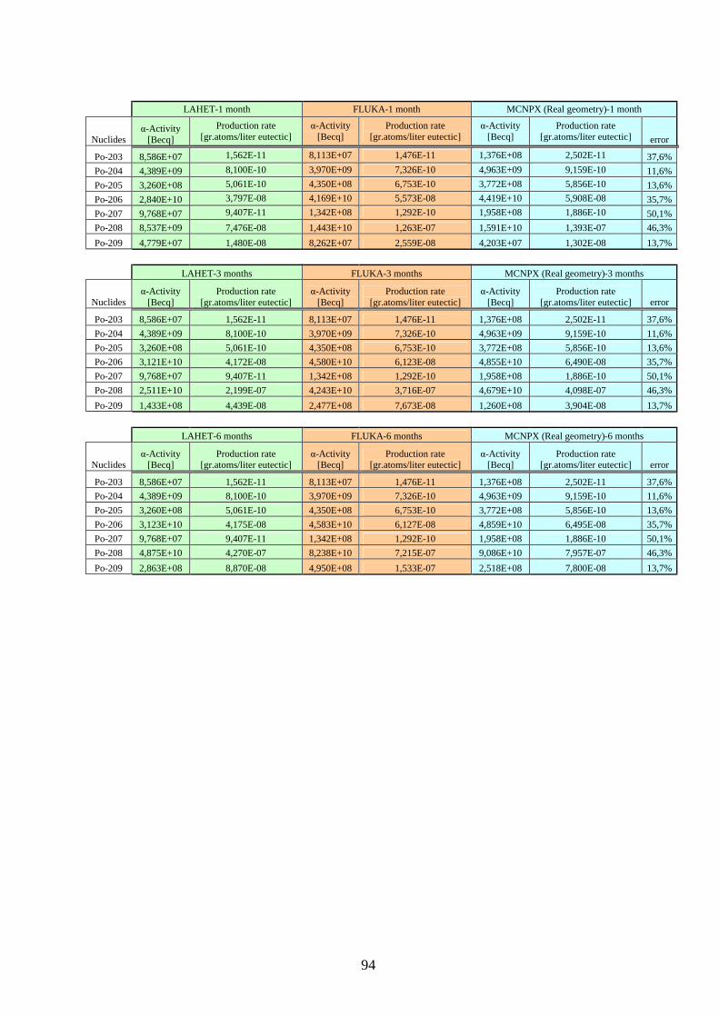
94
LAHET-1 month FLUKA-1 month MCNPX (Real geometry)-1 month
Nuclides α-Activity
[Becq] Production rate
[gr.atoms/liter eutectic] α-Activity
[Becq] Production rate
[gr.atoms/liter eutectic] α-Activity
[Becq] Production rate
[gr.atoms/liter eutectic] error
Po-203 8,586E+07 1,562E-11 8,113E+07 1,476E-11 1,376E+08 2,502E-11 37,6% Po-204 4,389E+09 8,100E-10 3,970E+09 7,326E-10 4,963E+09 9,159E-10 11,6% Po-205 3,260E+08 5,061E-10 4,350E+08 6,753E-10 3,772E+08 5,856E-10 13,6% Po-206 2,840E+10 3,797E-08 4,169E+10 5,573E-08 4,419E+10 5,908E-08 35,7% Po-207 9,768E+07 9,407E-11 1,342E+08 1,292E-10 1,958E+08 1,886E-10 50,1% Po-208 8,537E+09 7,476E-08 1,443E+10 1,263E-07 1,591E+10 1,393E-07 46,3% Po-209 4,779E+07 1,480E-08 8,262E+07 2,559E-08 4,203E+07 1,302E-08 13,7%
LAHET-3 months FLUKA-3 months MCNPX (Real geometry)-3 months
Nuclides α-Activity
[Becq] Production rate
[gr.atoms/liter eutectic] α-Activity
[Becq] Production rate
[gr.atoms/liter eutectic] α-Activity
[Becq] Production rate
[gr.atoms/liter eutectic] error
Po-203 8,586E+07 1,562E-11 8,113E+07 1,476E-11 1,376E+08 2,502E-11 37,6% Po-204 4,389E+09 8,100E-10 3,970E+09 7,326E-10 4,963E+09 9,159E-10 11,6% Po-205 3,260E+08 5,061E-10 4,350E+08 6,753E-10 3,772E+08 5,856E-10 13,6% Po-206 3,121E+10 4,172E-08 4,580E+10 6,123E-08 4,855E+10 6,490E-08 35,7% Po-207 9,768E+07 9,407E-11 1,342E+08 1,292E-10 1,958E+08 1,886E-10 50,1% Po-208 2,511E+10 2,199E-07 4,243E+10 3,716E-07 4,679E+10 4,098E-07 46,3% Po-209 1,433E+08 4,439E-08 2,477E+08 7,673E-08 1,260E+08 3,904E-08 13,7%
LAHET-6 months FLUKA-6 months MCNPX (Real geometry)-6 months
Nuclides α-Activity
[Becq] Production rate
[gr.atoms/liter eutectic] α-Activity
[Becq] Production rate
[gr.atoms/liter eutectic] α-Activity
[Becq] Production rate
[gr.atoms/liter eutectic] error
Po-203 8,586E+07 1,562E-11 8,113E+07 1,476E-11 1,376E+08 2,502E-11 37,6% Po-204 4,389E+09 8,100E-10 3,970E+09 7,326E-10 4,963E+09 9,159E-10 11,6% Po-205 3,260E+08 5,061E-10 4,350E+08 6,753E-10 3,772E+08 5,856E-10 13,6% Po-206 3,123E+10 4,175E-08 4,583E+10 6,127E-08 4,859E+10 6,495E-08 35,7% Po-207 9,768E+07 9,407E-11 1,342E+08 1,292E-10 1,958E+08 1,886E-10 50,1% Po-208 4,875E+10 4,270E-07 8,238E+10 7,215E-07 9,086E+10 7,957E-07 46,3% Po-209 2,863E+08 8,870E-08 4,950E+08 1,533E-07 2,518E+08 7,800E-08 13,7%
95
Bibliography [1] The European Technical Working Group on ADS, A European Roadmap for Developing Accelerator Driven Systems (ADS) for Nuclear Waste Incineration, April 2001. [2] C. Rubbia et al., Conceptual design of a fast neutron operated high power energy amplifier, CERN/AT/95-44 (ET), 1995. [3] http://aaa.lanl.gov/ [4] http://www.pnl.gov/atw/ [5] http://www.europhysicsnews.com/full/06/article8/article8.html [6] J. Cugnon et al., Nucl. Phys. A, 620, 475 (1997). [7] K. H. Schmidt et al., Nucl. Phys. A, 665, 221 (2000). [8] J.-J. Gaimard, K.-H.Schmidt; Nucl. Physics A, 531, 709 (1991). [9] T. Auger, Y. Bortoli, A. Cadiou, T. Kirchner, J.S. Stutzman (Subatech), Y. Dai, S. Dementjev, K. Geismann, F. Gröschel, F. Heinrich, K. Kohlik, G. von Holzen, Ch. Perret, D. Viol (PSI), H. Glasbrenner (FZK), Design Report for the LiSoR project, 2001. [10] http://inrwww.fzk.de/~inr487/public_html/megapie.pdf [11] C.H.M. Broeders, PhD thesis, Entwicklungsarbeiten für die neutronenphysikalische Auslegung von Fortschrittlichen Druckwasserreaktoren (FDWR) mit kompakten Dreiecksgittern in hexagonalen Brennelementen, Forschungszentrum Karlsruhe, 1992. [12] E. Stein, E. Wiegner, C. Broeders, Kurzbeschreibung des KAPROS-Moduls BURNUP, interne KAPROS-Notiz, 1982. [13] F. Atchinson, H. Schaal, ORIHET3, Version1.12, A guide for users, May 2002. [14] W. M. Brobeck, E. O. Lawrence et al., Phys. Rev., 71 (number 7), 449 (1947). [15] J. Taieb, PhD thesis, Etude de la production de noyaux résiduels d´évaporation issus de la réaction de spallation de l´uranium-238 par des protons á 1 GeV, Université de Paris Sud, INP-CNRS Orsay, October 2000. [16] http://www.cea.fr/fr/Publications/Clefs46/clefs46fr/clefs46_35.html
96
[17] A. Boudard, J. Cugnon, S. Leray, C. Volant, Intranuclear Cascade for a comprehensive description of spallation reaction data, December 3, 2001. [18] R. Serber, Phys. Rev., 72, 1114 (1947). [19] http://lpsc.in2p3.fr/reacteurs-hybrides/atelier_gedeon/Cugnon/Cugnon02.html [20] H.W. Bertini, Phys.Rev.,88,1711 (1969). [21] H.W. Bertini, Phys.Rev., 31,1801 (1963). [22] V. S. Barashenkov et al.,. Sov. Phys., Usp 16, 31 (1973). [23] V. Baylac-Domengetroy, Diplomarbeit, Investigations Related to the Generation of Reaction Products in the Target of Accelerator Driven Systems for Nuclear Waste Incineration, Forschungszentrum Karlsruhe, FZKA 6908, 2003. [24] A. Boudard et al., Phys. Rev. C, 66, 044615 (2002). [25] I. Broeders, Private communication. [26] C. Villagrasa-Cantón, PhD thesis, Etude de la production de noyaux résiduels dans la réaction de spallation Fe+p à 5 énergies (300-1500 MeV/A) et applications au calcul de dommages sur une fenêtre de système hybride, Université Paris XI Orsay, December 2003. [27] B. Fernandez-Dominguez, PhD thesis, Etude de la production des fragments de fission de la réaction 208Pb+p à 500 AMeV, Université de Caen, March 2003. [28] V. F. Weisskopf, Phys.Rev., 52, 295 (1937). [29] V.F. Weisskopf, D. H. Ewing, Phys.Rev., 57, 472 (1939). [30] A. R. Junghans et al., Nucl. Phys. A, 629, 635 (1998). [31] E. Vogt, Single neutrons halos in the valley of stability, Vancouver, May 2002. [32] A. Boudard, Private communication. [33] L. S. Waters, MCNPX user´s manual, Version 2.4.0, September 2002. [34] R. E. Prael, H. Lichtenstein, User Guide to LCS: The LAHET Code System, LANL, September 1989. [35] J. S. Hendricks, G. W. McKinney, L. S. Waters et al., MCNPX extensions, Version 2.5.0, February 2004. [36] J. S. Hendricks, G. W. McKinney, L. S. Waters et al., MCNPX extensions, Version 2.5.d, August 2003. [37] E-mail exchange with the SPhN (Service de Physique Nucléaire) at the CEA of Saclay. [38] http://dpnc.unige.ch/atlas/xin/noyaux/pdf/chapitre-2.pdf [39] http://www.carleton.ca/~dwiles/CRNL/section_one.htm
97
[40] H. A. Bethe, Phys. Rev., 54, 436 (1938). [41] W. H. Barkas, Phys. Rev., 55, 961 (1939). [42] L. Sihver et al., Phys. Rev. C, 47, 1225 (1993). [43] S. Kox et al. Phys. Rev. C, 35, 1678 (1987). [44] Shen et al. Nucl. Phys. A, 491, 130 (1989). [45] R. K. Tripathi et al., NASA Technical Paper, 3621 (1997). [46] Y. E. Titarenko, Experimental and theorical study of the yields od residual product nuclei produced in thin targets irradiated by 100-2600 MeV protons, ISTC, February 2001. [47] http://www-wnt.gsi.de/kschmidt [48] T. Enqvist et al., Nucl.Phys.A, 686, 481 (2001). [49] Y. E. Titarenko, private communication. [50] L. Audouin, PhD thesis, Dépendence en énergie des spectres isotopiques de résidus de spallation, Université de Paris 6, September 2003. [51] http://www.ganil.fr/eurisol/TOWN_MEETING_ABANO/ThomasKirchener.pdf [52] H. Glasbrenner et al., First irradiation experiment at the LiSoR loop, PSI. [53] Y. Foucher (Subatech), M. Pepin (PSI), M. Embib (Ciemat), Nuclear Assessment of the LiSoR project, 2000. [54] M. Pepin, Production of α-Radioactivity by 72 MeV protons on lead-bismuth eutectic and subsequent radiotoxic risk by evaporation of Pb-Po from open liquid surfaces, PSI. [55] P. Trabuc, the problem of polonium contamination in the MEGAPIE spallation target, CEA, 2001. [56] http://atom.kaeri.re.kr/ton/ [57] H. Glasbrenner, J. Eikenberg, F. Gröschel, L. Zanini, Irradiated Pb-55.5 Bi, PSI, 2003. [58] http://asq.web.psi.ch/ASQ/facilities/SINQSYSTEMS.html [59] http://sinq.web.psi.ch/ [60] U. Fischer, H. W. Wiese, Verbesserte konsistente Berechnung des nuklearen Inventars abgebrannter DWR-Brennstoffe auf der Basis von Zell-Abbrabd-Verfahren mit KORIGEN, KfK 3014 (1983). [61] M. J. Bell, ORIGEN- The ORNL Isotope Generation and Depletion Code, ORNL-4628 UC-32 (1973).
98
Validation of Calculation Tools for the Estimation of Reaction Products in the Target of Accelerator Driven Systems
Summary The spallation reactions have recently gained considerable interest due to their importance in technical applications. The spallation reactions generate a lot of neutrons and they can, for example, be used as spallation neutron sources. This property can be utilized in an Accelerator Driven System (ADS) which is composed of a neutron source, a spallation target and a sub-critical reactor. Thanks to the external neutron source, this application will allow to produce energy with higher safety and to incinerate nuclear waste. Actually several experimental research programs are running in order to realized the final construction of a hybrid system prototype: MUSE, TRADE, MYRRHA, MEGAPIE. A working tool to simulate the spallation reaction is provided to us. The MCNPX code (Monte Carlo with N Particles eXtended), is developed at the LANL and it is used actually at the IRS within the framework of the beta-testing. First we analyzed the new models INCL4 and ABLA recently integrated in the new version 2.5e of MCNPX in comparison with the original codes of J. Cugnon and K. H. Schmidt. It allows us to recommend the input parameters defining the pysical models and the corresponding normalizations. Moreover the influences of different input parameters on the spallation cross sections are quantified. We investigated the agreement of this code options with the experimental data from the GSI and ISTC groups at 1 GeV, with new data from the ISTC group at 600 MeV and with recently available data at 500 MeV from the GSI group. Further we studied the decay of isotopes in a LiSoR target experiment (Liquid metal Solid metal Reaction) in order to estimate the activity of residual spallation products which are radiotoxic as the Polonium 209. The last part of this work is devoted to the study of two codes which calculate the decay of isotopes: The modul BURN0D of the KAPROS system and the ORIHET3 code. The physical principles and theire use are discussed.
99
Validierung von Rechen-Programmen zur Abschätzung von Reaktionsprodukten im Target von Beschleuniger-Getriebenen Systemen
Zusammenfassung
Vor kurzem haben Spallations-Reaktionen beträchtliches Interesse wegen ihrer Bedeutung für technische Anwendungen gewonnen. Die Spallations-Reaktionen erzeugen viele Neutronen und sie können zum Beispiel als Spallations-Neutronenquellen verwendet werden. Diese Eigenschaft kann in einem Beschleuniger-gesteuerten unterkritischen System (ADS) benutzt werden, welches aus einer Neutronenquelle, einem Spallations-Target und einem unterkritischen Reaktor besteht. Diese Anwendung ermöglicht, wegen der externen Neutronenquelle, Energie mit höherer Sicherheit zu produzieren und nukleare Abfälle zu verbrennen. Zur Zeit laufen mehrere experimentelle Forschungs Programme, um zum Aufbau eines Prototyps für ein hybrides Systems zu führen: MUSE, TRADE, MYRRHA, MEGAPIE. Ein Arbeitswerkzeug steht uns zur Verfügung, um die Spallation Reaktion zu simulieren. Dieser Code, genannt MCNPX (Monte-Carlo mit N Partikeln eXtended), wird am LANL entwickelt und er wird am IRS im Rahmen des Beta-Tests verwendet. Zuerst haben wir die neuen Modelle INCL4 und ABLA, die vor kurzem in der neuen Version 2.5e von MCNPX integriert wurden, im Vergleich mit den Ursprungscodes von J. Cugnon and K. H. Schmidt analysiert. Das hat uns ermöglicht, die geeigneten Eingabe Parameter und Normalisierungen zu bestimmen. Außerdem sind die Einflüsse der unterschiedlichen Eingangs-Parameter auf die Spallations Querschnitte quantitativ bestimmt. Weiter haben wir die Übereinstimmung der Ergebnisse dieser Codes mit den experimentellen Daten von den gruppen GSI und ISTC bei 1 GeV, mit die neuen Daten von der Gruppe ISTC bei 600 MeV und mit ganz neu verfügbaren Daten von GSI bei 500 MeV untersucht. Dann haben wir den Zerfall der Isotope im Rahmen des LiSoR Projekts (Liquid metal Solid metal Reaction) studiert um die Aktivitäten der Spallationprodukte abzuschätzen, die wie zum Beispiel Polonium 209 radiotoxisch sein können. Der letzte Teil dieser Arbeit befasst sich mit zwei Codes, die den Zerfall von Isotopen berechnen. Der Modul BURN0D aus dem KAPROS System und der ORIHET3 Code. Die physikalische Grundlagen und die Benutzung dieser Programme sind dort erläutert.
100
Validation des Outils de Calcul pour l’Estimation des Produits de Réaction dans la Cible d’un Système Sous-Critique Piloté par Accélérateur
Résumé
Les réactions de spallation ont récemment connu un regain d’intérêt considérable grâce à leur importance dans les applications techniques. Les réactions de spallation sont en effet très neutrogènes et elles peuvent, par exemple, être employées en tant que sources de neutrons de spallation. Cette propriété peut être utilisée dans un système sous-critique piloté par accélérateur (Accelerator Driven System, ADS) qui est composé d’une source de neutron, d’une cible de spallation et d’un réacteur sous-critique. Grâce à cette source extérieure de neutrons, cette application permet de produire de l’énergie avec une augmentation de la sûreté et d’incinérer des déchets nucléaires. Actuellement plusieurs programmes expérimentaux de recherche sont en cours afin d’arriver à la construction finale d’un démonstrateur de système hybride : MUSE, TRADE, MYRRHA, MEGAPIE. Nous avons à notre disposition un outil de travail pour simuler la réaction de spallation. Ce code, appelé MCNPX (Monte Carlo avec N Particules eXtended), est développé au LANL et il est employé actuellement à l’IRS dans le cadre du beta-testing. D’abord nous avons analysé les nouveaux modèles INCL4 et ABLA récemment intégrés dans la nouvelle version 2.5e de MCNPX en comparaison avec les codes d’origine de J. Cugnon et K. H. Schmidt. Cela nous a permis de comprendre et déterminer les paramètres d’entrée définissant les modèles physiques ainsi que les normalisations correspondantes. De plus, l’influence de certains paramètres d’entrée sur les distributions de spallation a été évaluée. Ensuite nous avons étudié la concordance de ces codes avec les données expérimentales des groupes GSI et ISTC à 1 GeV tout d’abord, puis avec les nouvelles du groupe ISTC à 600 MeV et enfin avec des données du groupe GSI à 500 MeV obtenues très récemment. Ensuite nous avons étudié la décomposition des isotopes dans une cible définit par le projet LiSoR (Liquid metal Solid metal Reaction) afin d’estimer l’activité des produits résiduels de spallation qui peuvent être radiotoxiques comme le Polonium 209, par exemple. La dernière partie de ce travail est dédiée à l’étude de deux codes calculant la décomposition des isotopes : Le module BURN0D du système KAPROS et le code ORIHET3. Les principes physiques de leur fonctionnement ainsi que leur utilisation y sont développés.