Valuing Government Guarantees

in Toll Road Projects

Luiz E. T. Brandão1 e Eduardo C. G. Saraiva2

Rio de Janeiro

This version: March/2007

1 Professor at Pontifical Catholic University of Rio (PUC-Rio), IAG Business School. (www.iag.puc-rio.br). Rua

Marquês de São Vicente, 225, Gávea, Rio de Janeiro, RJ, (brandao@iag.puc-rio.br)

2 Doctoral student EPGE/Fundação Getulio Vargas (www.epge.fgv.br). Praia de Botafogo 190, 11o andar, Botafogo, Rio de Janeiro, (eduardo@fgvmail.br). National Bank for Economic and Social Development (BNDES).(www.bndes.gov.br). Av. República do Chile, 100, 19º andar, Centro, Rio de Janeiro, RJ. (eduardo.saraiva@bndes.gov.br).

Valuing Government Guarantees in Toll Road Projects

Luiz E. T. Brandão1 and Eduardo C. G. Saraiva2

Abstract

The participation of private capital in public infrastructure investment projects has been sought by many governments who perceive this as a way to overcome budgetary constraints and foster economic growth. For some types of projects, this investment may require government participation in the form of project guarantees in order to reduce the risk of the private investor. As a consequence, the government assumes a contingent liability which may have significant future impact. For this reason, the risk analysis and valuation of these guarantees is important for both the private investor and the government. We present a real options model than can be use to assess the value of these guarantees, allows the government to analyze the cost/benefit of each level of support, and propose alternatives to limit the exposure of the government while still maintaining the benefits to the private investor. This model is then applied to the proposed BR-163 toll road that will link the Brazilian Midwest to the Amazon River. We conclude that a minimum traffic guarantee combined with a cap on the total government outlays for the project offers the best combination of risk reduction for the private investor and liability limits for the government.

Keywords: Real Options, Toll Roads, Government Guarantees, Valuation, Finance

1 Professor, Pontifical Catholic University of Rio (PUC-Rio) IAG Business School (www.iag.puc-rio.br). Rua Marquês de São Vicente, 225, Gávea, Rio de Janeiro, RJ, Brazil

brandao@iag.puc-rio.br, (55 21) 2138-9304

2 Doctoral student, Fundação Getulio Vargas/EPGE (www.epge.fgv.br). Praia de Botafogo 190, 11o andar, Botafogo, Rio de Janeiro eduardo@fgvmail.br National Bank for Economic and Social Development (BNDES).(www.bndes.gov.br). Av. República do Chile, 100, 19º andar, Centro, Rio de Janeiro, RJ. eduardo.saraiva@bndes.gov.br.

1

Introduction

The 1990’s was characterized by a worldwide trend towards an increase in participation

of private investment in public infrastructure projects in substitution of government investment,

the main motivation being the gains in efficiency derived from the substitution of public

administration for private enterprises, a better allocation of risk and budgetary constraints of

governments. On the other hand, private infrastructure projects are subject to government

regulation, cover services deemed essential by society, require large amounts of irreversible

capital investment, have long maturity time and are usually offered monopolistically. This

combination of factors assures that, once implemented, the interests of the government and that

of the private investor begin to diverge, which subjects these projects to pressure from users and

opportunist behavior by the government, increasing the risk to the investor. Due to this, private

investors may demand that the government provide guarantees that have the effect of reducing

these risks, and in doing so, turn the government into a stakeholder in the project.

Government guarantees have been used frequently in private infrastructure projects. The

World Bank aided the government of Colombia to structure the El Cortino-El Vino toll road

concession where traffic and construction cost guarantees were offered. For the expansion of the

gas fired energy plant of Barranquilla, at a cost of $755 million dollars, the Colombian

government guaranteed that the state owned Public Utility Company would honor a take or pay

contract. (Beato, 1997, Lewis and Moody, 1998). The concession of the Santiago-Valparaíso-

Viña del Mar toll road in 1998, with 130 km and a cost of $400 million dollars, offered a

minimum traffic guarantee at an additional cost to the investor. (Engel, Fisher and Galetovic,

2000). The Linha Amarela expressway in Rio de Janeiro, in 1994, also includes a grant of US$

112 million, for a total project value of US$ 174 million (Dailami and Klein, 1997).

The presence of the government as mitigator of risk may be a necessary condition since

the control of many of the variables that affect important aspects of the project are under its

responsibility, such as interest rates, regulation and others, because market risk is such that the

project is not feasible from the perspective of the private investor. An example was the bid of the

Costanera Norte toll road in Chile in 1998, a urban highway of 30 km connecting the city of

Santiago to the airport, in which the government initially refused to offer guarantees deemed

necessary by the private investors. Consequently, no bids were forwarded. Only after

government supports were included was the road was successfully bid.

2

On the other hand, by offering guarantees for infrastructure projects, the government

becomes responsible for all future liabilities that these supports may cause, and which, because

they are determined subjectively in most cases, are not adequately valued or even accounted for

in government budgets. This can become very onerous to the government if the risks involved

are not adequately analyzed and quantified. The foreign exchange guarantees provided by the

Spanish Government in the 1970’s and the failure of the Mexican toll road concessions after the

1994 Mexican crisis eventually cost $2.5 billion and $8.9 billion respectively to these

governments. Thus, the importance of the valuation of government supports is that it allows the

government to define a level of guarantee that is high enough for the project to be economically

feasible, but low enough not to burden the government and society in excess, and also to

determine the value of budgetary and fiscal impacts of future contingent liabilities.

Government supports have option like characteristics, and determining the optimal level

of these guarantees requires the use of option pricing methods, which cannot be achieved

through traditional project analysis methods. Brandão (2002) applied real option valuation on a

model of the Via Dutra highway in Brazil that incorporates the value of options to expand and to

abandon. Ng and Björnsson (2004) present arguments in favor of the use of real option approach

to the analysis of a toll road concession project. Rose (1998) shows that the value of the

Melbourne Central Toll project in Australia increases considerably when the value of the

flexibility to increase revenues is considered. Bowe and Lee (2004) analyze the Taiwan High-

Speed Rail project where the concessionaire has the option to develop real estate projects along

the right of way and show that the value of these options greatly reduces the risk of the project.

On the other hand, the literature on the valuation of government supports is scarce.

Charoenpornpattana et.al (2002) analyze a minimum traffic guarantee and shadow toll as a

bundle of independent options, but their model uses project cash flows as the underlying asset

rather than traffic. Lewis and Mody (1997) and Irwin (2003) mention a World Bank study to

value traffic guarantees that were offered in the El Cortijo-El Vino toll road in Colombia using

option-pricing methods.

In this paper we propose a model for the valuation of revenue or traffic guarantee in a toll

road project, and an estimate of the expected value of the government outlays under these

guarantees under various conditions. This paper differs from Charoenpornpattana et.al (2002) in

that we model the exercise of the options directly over traffic levels rather than project cash

3

flows in order to more accurately reflect the impact of the government guarantees, and show how

multiple sources of uncertainty as well as limits to the government outlays can also be included.

Through a real options analysis we determine the value of guarantees which may be offered by

the government, their impact of the reduction of risk of the project and the expected value of

future government payments as function of the level of the guarantees and limitations these

guarantees may be subject to. This allows governments to maximize return to society by

designing a bid contract which incorporates the value of these supports.

This work is organized as follows. The first section presents this introduction and a

summary of the main topics. In the second section we discuss possible types of government

infrastructure concessions projects and their impact on private sector risk. In the third section, we

present a real option valuation model for private infrastructure projects, and in the next section

we illustrate this with an application to the BR-163 toll road project. In section five we conclude.

2 – Toll Road Concession Models

Toll road concession contracts can be classified according to the degree of risk the private

investor is subjected to. In a traditional concession, all market risk are transferred to the

concessionaire while the government provides no supports and holds no future liabilities, and

this risk is reflected in a higher risk premium for the private capital. This is the most widely used

type of concession, prevalent in the Argentina, Brazil, Chile and the United States, and is based

on the build, operate and transfer (BOT) model (Bousquet and Fayard (2001), Hammami,

Ruhashyankiko and Yehoue (2006)). According to the World Bank (2006), more than 160 such

projects totaling 37 billion dollars of concessions were granted in Latin America and the

Caribbean between 1990 and 2005. In the United States, 4.000 miles of toll road concessions for

the US$ 100 billion dollar Trans Texas Corridor and portions of the highway I-35 are currently

under construction or being auctioned (Persad et al., 2004).

This model generally breaks down when the project risk is deemed so high or the returns

so uncertain that the government is unable to attract private capital for the project. This typically

happens because governments usually grant out concessions of the most profitable projects first,

and after this stock is depleted is left with less attractive high risk low return projects. One

solution for this problem is to grant some level of government support that reduces the risk

4

and/or increases the returns to the private investor. In Brazil in the XIX century (Summerhil

(1998, 2003)), equity guarantees were given in order to foster private investment in

transportation infrastructure such as railroads with great success1. More recently, in 2004 the

Brazilian Congress voted Law 11.079/04, which allows the government to grant supports to

infrastructure projects known as Public-Private-Partnerships (PPP).

PPP’s have been in use by governments worldwide to increase their global efficiency and

due to the lack of investment capital due to budgetary restrictions. Under this model, for

example, if the returns of the project are much lower than expected, the project may receive a

government subsidy proportional to the reduction in the observed demand, so that a minimum

level of return is maintained. Other options may also be present, such as the option to extend (or

contract) the concession period, or to postpone payments due to the government. On the other

hand, PPPs require a long term commitment of the government to a project, along with the risk

of taking on future liabilities that are usually not sufficiently accounted or adequately quantified.

The indiscriminate granting of government supports can become a heavy burden to society,

because by offering these options the government creates future liabilities and potential

responsibilities. Even though they may not bear any impact on current cash flows, government

supports may pose a heavy cost for future generations, since the cost of these outlays are rarely

taken into consideration or even included into the budgeting process due to the limitations of the

traditional valuation methods.

The participation of the government as guarantor of last resort gives it an important role

in the implementation of projects that may be technically sound but not economically feasible

under the classical model of concession analysis. This objective may be reached by offering

guarantees that limit the losses and reduce the risk of the concessionaire in order to allow the

implementation and continuity of the project. Government support in PPP contracts can take on

many forms, from a simple extension of the concession period to a guarantee of a specific project

NPV or a minimum return on the invested capital, representing different levels of risk reduction.

When the government offers minimum revenue of traffic guarantees, it eliminates the

most unfavorable states of the distribution of the returns of the project. This fact produces two

distinct effects: on one hand, it increases the average return, on the other; it reduces the risk of

1 These guarantees were also provided to industrial projects. In March 24, 1881, the Imperial Government of Brazil

granted a 7% yearly equity guarantee for the construction of a sugar mill in the village of Bracuhy, Rio de Janeiro.

5

the project by eliminating payoffs below a certain level. Reducing the risk of the project reduces

the discount rate at which the cash flows must be discounted, which increases the project value.

Another model that can also be adopted is the Develop, Build, Finance and Operate

(DBOF) model used in Great Britain and Portugal, where the government pays out a

contractually established yearly revenue stream directly to the concessionaire, and which may or

may not involve the collection of tolls from the users. Since in this model the government bears

the totality of the market risk, there is no risk to the private investor and a competitive auction

for the award of the concession is likely to produce the lowest revenue stream to be paid out,

reflecting a significantly lower risk premium for the private capital. On the other hand, in case of

an economic downturn the government is obligated to cash outlays at a time where its budget is

under greater pressure.

3 – Risk Analysis and Modeling

Toll road projects offer many distinct sources of risk to the investor (Fishbein and Babbar

(1996)). Many of these are private, diversifiable risks, which we assume are of less concern to an

adequately diversified investor, such as construction risk, or risks which can be hedged away,

even if at a cost, such exchange rate risk. On the other hand, the uncertainty over the future

levels of demand for traffic on the completed road is of great consequence and constitutes an

undiversifiable market risk.

We assume there is a contractual guarantee where the government is obligated to make

certain payments to the concessionaire whenever the traffic level (AADT – Average Anual Daily

Traffic) falls below a pre-established floor during a period of time. If we assume that the toll rate

is constant throughout the concession period, then the traffic guarantee is equivalent to a revenue

guarantee.

Let Rt be the observed revenue of the project (Rt = AADTt x Toll Rate) in year t and Pt the

minimum revenue guaranteed by the government in that year. Since we assume that the toll rate

is constant, the stochastic processes of traffic and revenues will have the same parameters, so we

are indifferent whether one or another is used as the underlying asset. In this case, considering

the guarantee received, the effective revenue for the concessionaire in year t will be:

6

R(t) = max (Rt, Pt)

Similarly, the value G(t) of the government guarantee in that year will be:

G(t) = max (0, Pt – Rt) (1)

Given the uncertainty about the future level of traffic and revenues, in order to model this

variable we consider that the traffic and the revenue vary stochastically in time, following a

Geometric Brownian Motion (GBM), as is usual in the literature. This model implies that the

revenue can never be negative and that its volatility is constant in time and can be represented as:

RdR Rdt Rdzα σ= + (2)

where dR is the incremental change in revenue during a short period of time dt,

α is the revenue growth rate in a short interval of time dt,

σR is the volatility of the revenue

dz dtε= , where (0,1)Nε ∼ is the standard Wiener process.

It can be shown through an Ito process that this GBM can be represented by the

stochastic evolution of the returns, as shown in Equation (3), which can be discretely modeled in

yearly periods as a function of the value in the previous period, as shown in Equation (4). 2

ln2

RRd R dt dzσα σ

⎛ ⎞= − +⎜ ⎟⎝ ⎠

(3)

2( )

21

Rt Rt t

t tR R eσα σ ε− ∆ + ∆

+ = (4)

This process can be completely specified considering only its initial value R0, a yearly

growth rate and the volatility of the process, which we assume to be constant during the

concession period, where Equation (2) represents the “true” process of the evolution of the

project revenues. To value the guarantees, on the other hand, we must use a risk neutral process

where we subtract the risk premium from the expected return rate of the underlying asset,

substituting its “true” return by the risk free rate of return.

Given that neither the revenues nor the traffic are market assets, we cannot determine the

appropriate market risk premium for this source of uncertainty directly from market data. Some

7

authors, such as Irwin (2003) and Dixit and Pindyck (1994) suggest an exogenous solution where

an arbitrary value for the risk premium is adopted. We show that the parameters for the risk

premium of the revenues can be estimated from the stochastic process of the value of the project.

Let us assume that the revenue process is defined by Equation (2). Given that the

revenues represent the only source of project uncertainty, we can define the evolution of the

value of the project ( )V f R= subject to the same standard Wiener process dz where:

PdV Vdt Vdzµ σ= + (5)

where Pσ is the project volatility

By means of an Itô process, we can define:

22 2

2

12

P

R R

VV

V V V VdV R R dt R dzR t V R

σµ

α σ σ⎡ ⎤∂ ∂ ∂ ∂

= + + +⎢ ⎥∂ ∂ ∂ ∂⎣ ⎦ (6)

From CAPM we have ( [ ] )P mr E R rµ β= + − , where µ and Pβ are respectively the risk

adjusted discount rate and the Beta of the project. The risk premium of V(R) is then given by

( [ ] )P mr E R rµ β− = − . As we will see in this section, the risk premium of the project can also be

expressed as Pλσ , therefore we have:

Prµ λσ− = (7)

Substituting Equation (6) into (7) we remain with:

22 2

2

1 1 12 R R

V V V VR R r RR t V V R Vα σ λ σ

⎡ ⎤∂ ∂ ∂ ∂⎡ ⎤+ + − =⎢ ⎥ ⎢ ⎥∂ ∂ ∂ ∂⎣ ⎦⎣ ⎦ and

( )2

2 22

1 02R R

V V VR R rVR t V

α λσ σ∂ ∂ ∂− + + − =

∂ ∂ ∂ (8)

Equation (8) is the differential equation that the value of a project subject to revenue risk

must conform to. With this equation we can then determine the value of options on revenues or

project value, as long as we use a risk neutral process for the project revenues, with a drift rate of

Rα λσ− instead of α. Under the assumption that the value of the project without options is the

best unbiased estimate of its market value, from CAPM we can determine the risk premium of

the project cash flows. If µ is the expected rate of return of the project and βP is its Beta, then

8

[ ]( )P mr E R rµ β= + − and the project risk premium will be [ ]( )P mr E R rµ β− = − . Similarly,

the risk premium of the revenues is given by

[ ]( )R mr E R rα β− = − (9)

We define the market price of risk λR as RR

rαλσ−

= (10)

Substituting (10) and the value of ,2

m RR

m

σβ

σ= into Equation (9), multiplying both sides by

R

R

σσ⎛ ⎞⎜ ⎟⎝ ⎠

and re-arranging, we obtain [ ],

R

m R mR R R

m R m

E R r

ρ

σλ σ σ

σ σ σ⎛ ⎞−⎛ ⎞

= ⎜ ⎟⎜ ⎟⎝ ⎠⎝ ⎠

, where ρR represents the

correlation between the change in revenues and the market returns.

Finally, we remain with

[ ]mR R

m

E R rλ ρ

σ⎛ ⎞−

= ⎜ ⎟⎝ ⎠

(11)

In a similar way, the market price of risk λP of the project will be

[ ]mP P

m

E R rλ ρ

σ⎡ ⎤−

= ⎢ ⎥⎣ ⎦

(12)

where ρP represents the correlation between the project returns and the market.

Given that we assume that the only source of uncertainty of the project are its revenues,

the correlation ρR between the changes in revenues and the market returns will be identical to the

correlation ρP between the project returns and the market, which implies that (11) = (12), and λR

= λP = λ. From (9) and (10) we can then obtain [ ]( )R R mE R rλσ β= − , which defines the risk

premium of the revenues. In a similar fashion we can also obtain

[ ]( )P P mE R rλσ β= − (13)

Since the value of βR is unknown, we multiply both sides of equation (13) by R Pσ σ and

remain with Equation (14), which is the expression for the risk premium of revenues as a

9

function of the risk premium and volatility of the project and the volatility of the revenues, all of

which are known constants.

[ ]( ) RR P m

P

E R r σλσ βσ

= − (14)

The risk neutral process of revenues is then:

( )R RdR Rdt Rdzα λσ σ= − + (15)

where λσR is the risk premium of revenues previously determined in (14). We refer the

reader to Hull (2006) for a more extensive analysis of this property.

The uncertainty over future levels of traffic and revenues is one of the key parameters of

the model. For existing roadways, the volatility of the revenues can be observed from historical

series of traffic levels. For new roadways, this volatility can be estimated if we assume that

traffic levels and regional GDP are correlated. The project volatility can be determined from a

Monte Carlo simulation of the stochastic cash flows of the project. Due to the leverage effect of

project fixed costs, project volatility tends to be greater than traffic/revenue volatility, which

reduces the risk premium of revenues.

10

4 – Application

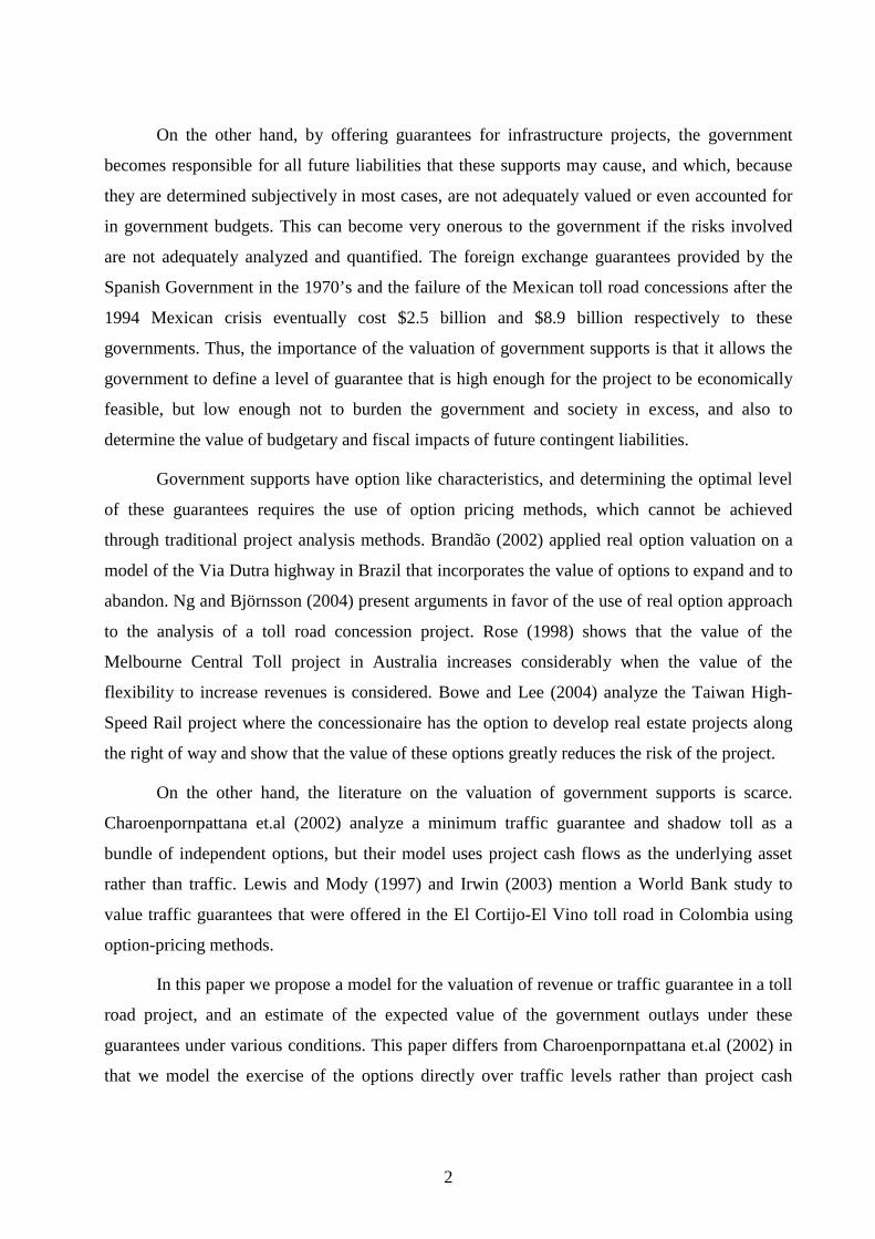
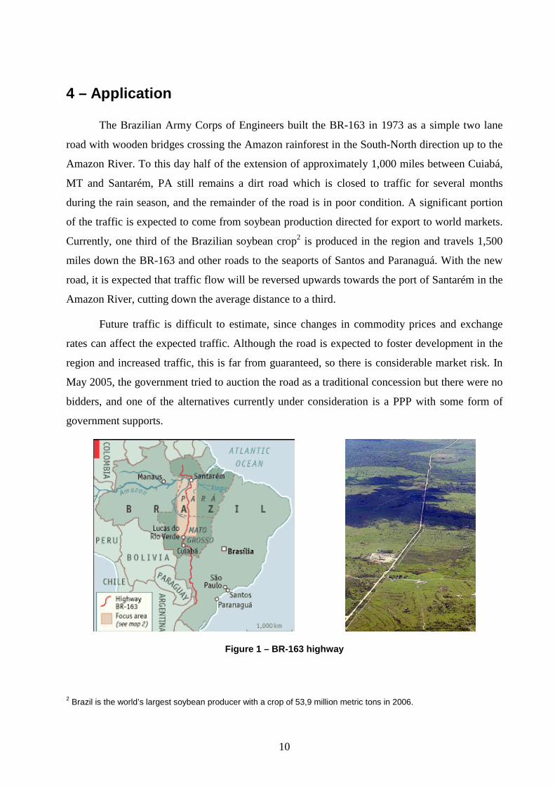
The Brazilian Army Corps of Engineers built the BR-163 in 1973 as a simple two lane

road with wooden bridges crossing the Amazon rainforest in the South-North direction up to the

Amazon River. To this day half of the extension of approximately 1,000 miles between Cuiabá,

MT and Santarém, PA still remains a dirt road which is closed to traffic for several months

during the rain season, and the remainder of the road is in poor condition. A significant portion

of the traffic is expected to come from soybean production directed for export to world markets.

Currently, one third of the Brazilian soybean crop2 is produced in the region and travels 1,500

miles down the BR-163 and other roads to the seaports of Santos and Paranaguá. With the new

road, it is expected that traffic flow will be reversed upwards towards the port of Santarém in the

Amazon River, cutting down the average distance to a third.

Future traffic is difficult to estimate, since changes in commodity prices and exchange

rates can affect the expected traffic. Although the road is expected to foster development in the

region and increased traffic, this is far from guaranteed, so there is considerable market risk. In

May 2005, the government tried to auction the road as a traditional concession but there were no

bidders, and one of the alternatives currently under consideration is a PPP with some form of

government supports.

Figure 1 – BR-163 highway

2 Brazil is the world’s largest soybean producer with a crop of 53,9 million metric tons in 2006.

11

We model the effects of a minimum traffic guarantee in order to determine the optimal

level of this guarantee and its cost to the government. This guarantee provides the

concessionaire the recourse to the government to receive compensatory payments whenever the

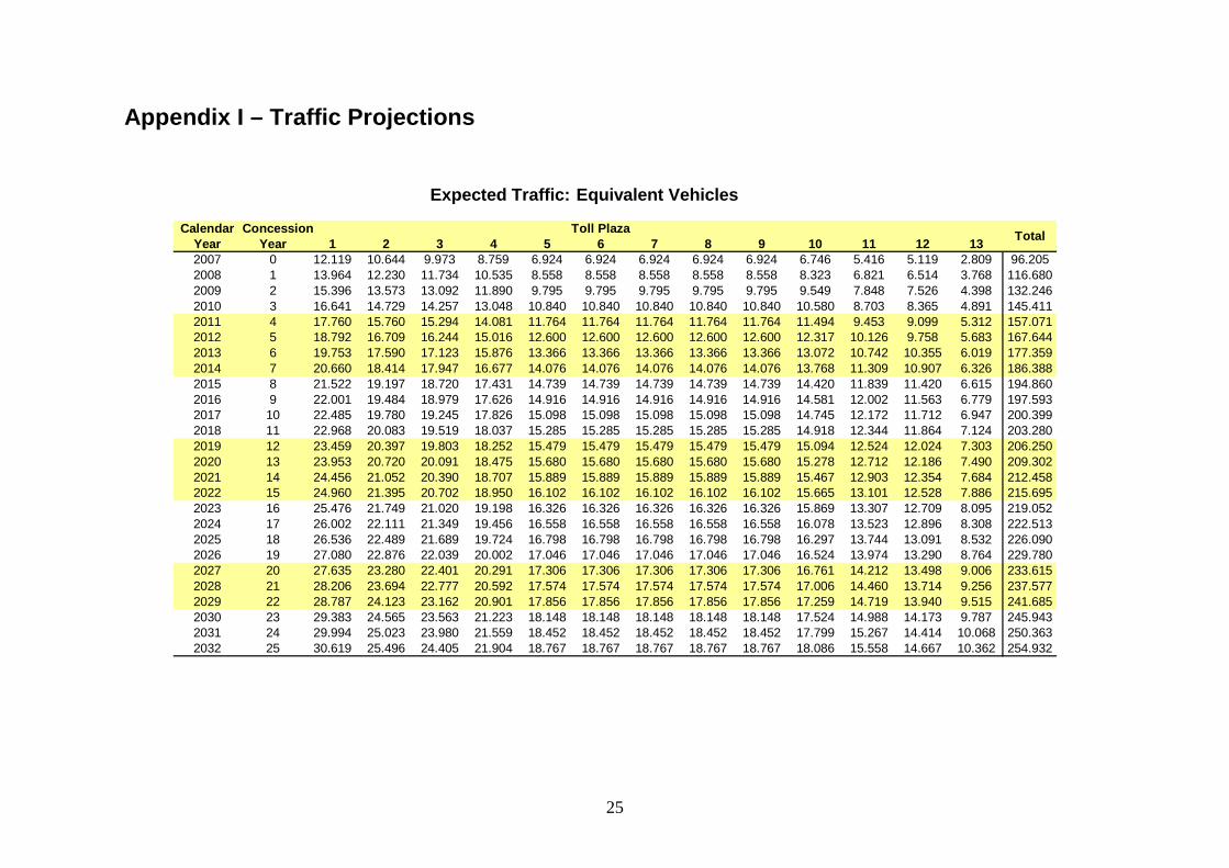
observed traffic and revenue is below a pre-established level. The traffic projections data used in

this paper (Appendix I) are official government estimates and are available at

www.tranportes.gov.br.

We assumed that concession year 0 is calendar year 2007, that the construction and

pavement of the roadway will last three years and that the first operational revenues will occur in

year 2, which corresponds to calendar year 2009. There will be no toll collection in year 1, and in

years 2 and 3 tolls will be collected only in the four toll plazas where construction work on the

road has been completed, representing 28% of the total flow of vehicles in these two years. From

the third year on the road is assumed to be completed and full toll revenues begin to be received.

The basic toll rate for a standard automobile adopted in this analysis is R$ 7.60 (approximately

US$ 3.50 at the current 2007 exchange rate) at each of the 13 toll plazas which are spread out at

approximately 120 km (80 miles) intervals. This represents a rate of R$ 0.06 per km (US$ 0.045

per mile), which is slightly below the current average of Brazilian toll roads. The time frame is

the full concession period of 25 years, so the starting year is 2007 (year 0) e the ending year is

2032 (year 25). We also assumed that the private investor cost of capital is 16% per year.

Project Model

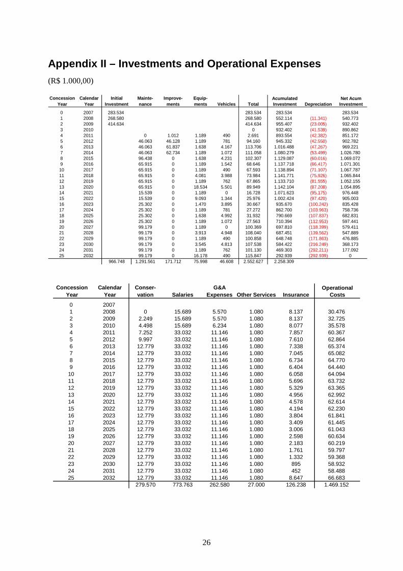
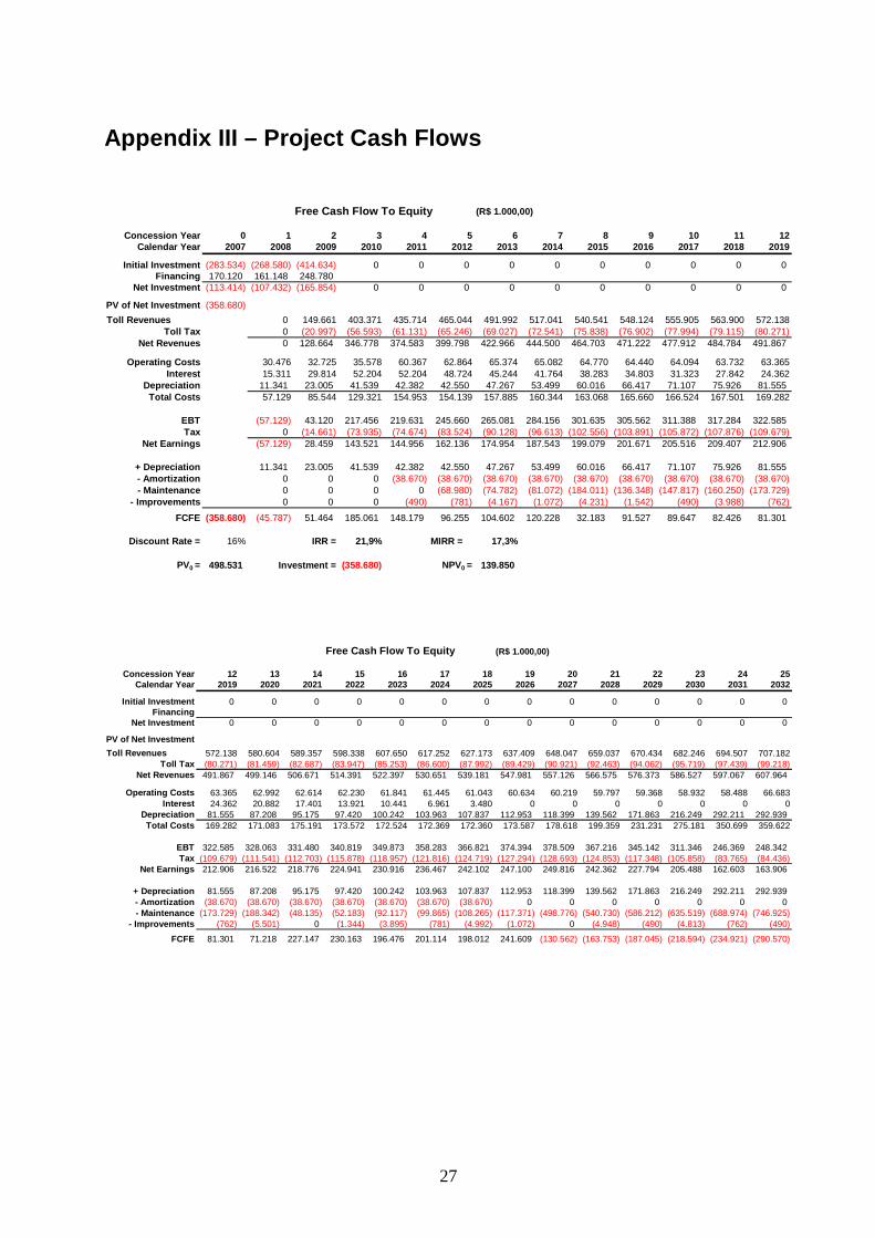
Appendix II and III show respectively the investment and operating expenses and the

static cash flow of the concession. The initial investment is R$ 966,7 million (USD $1 = R$

2.20) distributed along the first three years, and considering a debt level of 60%, traditional DCF

provides a NPV of R$ 139,8 million. These results indicate that while the project apparently is

economically feasible given that its NPV is positive, the result is not sufficient for the

concessionaire to undertake the project due to the difficulty of assessing the actual risks

involved.

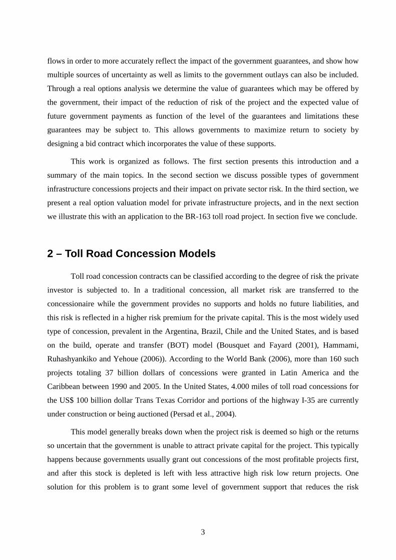
Given that there is no relevant historical traffic data for the road, the volatility of the

future traffic demand was estimated assuming a correlation with the regional GDP. Based on

12

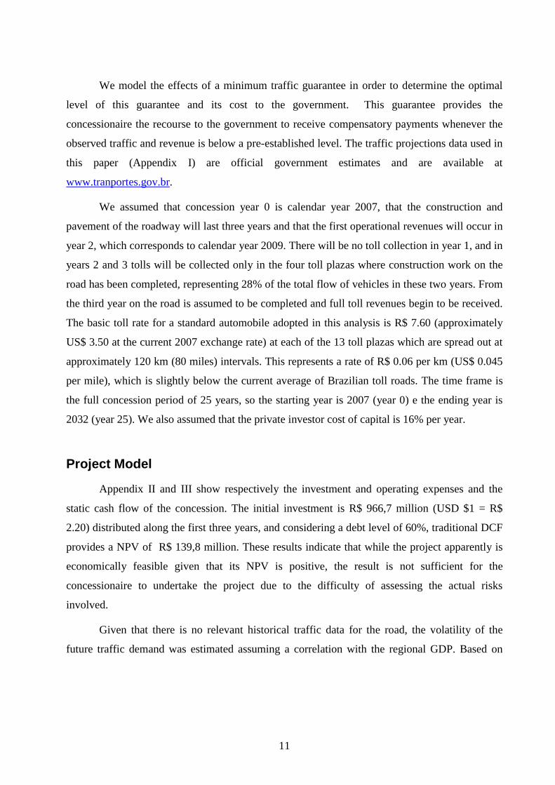
data from IPEA3, a government agency for economic analysis, the volatility of Brazil’s Midwest

GDP from 1980 to 2002 was 6.9% per year in average, and 7.0% between 1990 and 2002. We

assumed a traffic volatility of 7% per year

and an initial level of traffic of 106,894

Equivalent Daily Vehicles (EDV)4 for the

year 2007 for all thirteen toll plazas of the

roadway. Given that this initial traffic

volume is also uncertain, we assumed a

triangular probability distribution around this

value with a minimum of 74,826 and a

maximum of 138,962 EDV, corresponding to

a variation of ± 30%. (Figure 2).

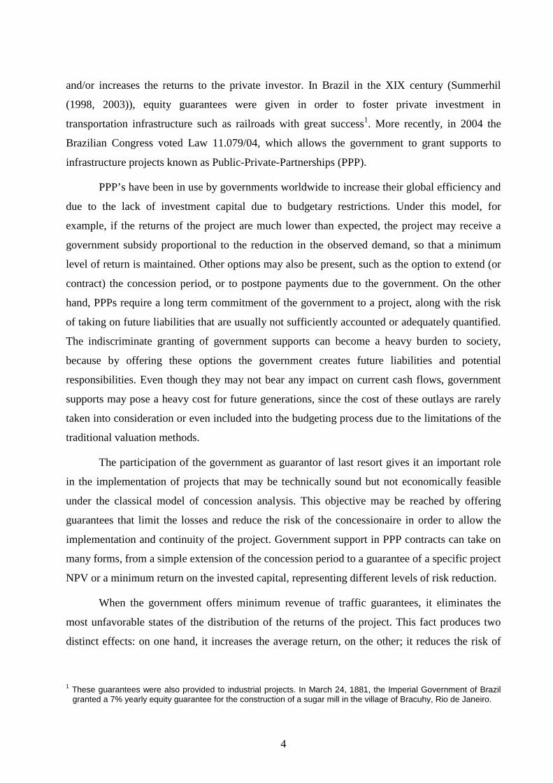
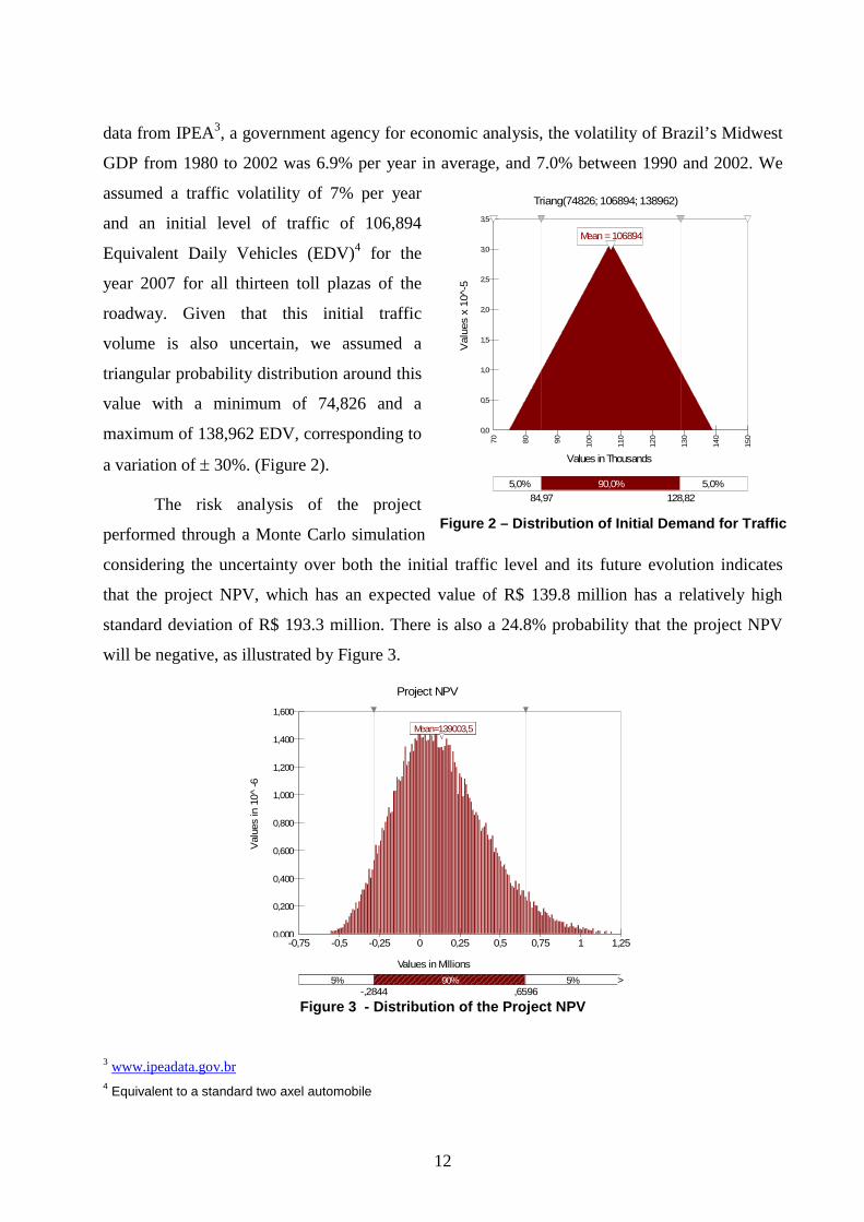
The risk analysis of the project

performed through a Monte Carlo simulation

considering the uncertainty over both the initial traffic level and its future evolution indicates

that the project NPV, which has an expected value of R$ 139.8 million has a relatively high

standard deviation of R$ 193.3 million. There is also a 24.8% probability that the project NPV

will be negative, as illustrated by Figure 3.

Project NPV

Val

ues

in 1

0 ̂-6

Values in Millions

0,000

0,200

0,400

0,600

0,800

1,000

1,200

1,400

1,600

Mean=139003,5

-0,75 -0,5 -0,25 0 0,25 0,5 0,75 1 1,25

-0,75-0,75

-0,75 -0,5 -0,25 0 0,25 0,5 0,75 1 1,25

5% 90% 5% > -,2844 ,6596

Mean=139003,5 Mean=139003,5

Figure 3 - Distribution of the Project NPV

3 www.ipeadata.gov.br 4 Equivalent to a standard two axel automobile

Triang(74826; 106894; 138962)

V

alue

s x

10^-

5Values in Thousands

0,0

0,5

1,0

1,5

2,0

2,5

3,0

3,5

70 80 90 100

110

120

130

140

150

5,0% 5,0%90,0%84,97 128,82

Mean = 106894

Figure 2 – Distribution of Initial Demand for Traffic

13

This analysis does not incorporate the value or the impacts on the project of any form of

government supports that could be offered to make it more attractive to private investors. As

shown before, in this concession model, the private investor holds all the project risk, which is

considerable, and the cost to the government is zero. Therefore, the private investor will require

a higher risk premium and consequently, a higher toll rate.

Valuation of Guarantees

The valuation of the government guarantees can be modeled as a series of independent

European options with maturities between 1 and 25 years. While in principle, these options can

be valued directly with the Black and Scholes equation, given that the traffic growth rate is non

constant, we chose to use simulation methods. Given the risk neutral process of the revenues

defined in (15), the value of the guarantee options can be determined by simulating different

future scenarios considering the possibility of exercising the option whenever the revenue value

falls below the minimum revenue. This option value is then discounted at the risk free rate. The

value of the concession with the revenue guarantee can then be obtained by simply repeating this

analysis for each of the 25 years of the concession and adding the present value of all these

options to the static value of the project, as shown in Equation (16).

25

1Value of Guarantee Value of Option i

i==∑ (16)

The volatility of the project is determined by a simulation of the stochastic project cash

flow adopting the criteria proposed by Brandão, Dyer and Hahn (2005b). The results indicate a

volatility of 47,8%. Assuming a risk free rate of 7%, the risk premium of the project cash flows

is can be determine from [ ]( ) 8%C mr E R rµ β− = − = , and from equation (14) we obtain a value

for the risk premium of the revenues (and traffic) of 1,32λ = . Given the risk neutral process of

the revenues defined in (15), we determine the value of the option considering the value of

exercise in each year, and the total aggregate value of all options during the concession period at

each level of guarantee.

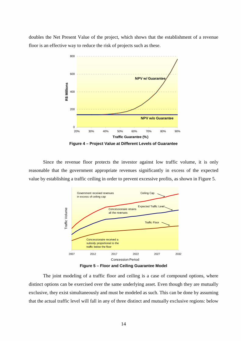
Figure 4 illustrates how the project value changes with each level of guarantee. A

contract guarantees that at least 60% of the expected traffic revenue will be received by the

investor, for example, increases the project value by R$ 101.9 million dollars, and this value

increases as the guarantee level increases. A guarantee level of 80% has a significant impact and

14

doubles the Net Present Value of the project, which shows that the establishment of a revenue

floor is an effective way to reduce the risk of projects such as these.

0

200

400

600

800

20% 30% 40% 50% 60% 70% 80% 90%

Traffic Guarantee (%)

R$

Mill

ions

NPV w/o Guarantee

NPV w/ Guarantee

Figure 4 – Project Value at Different Levels of Guarantee

Since the revenue floor protects the investor against low traffic volume, it is only

reasonable that the government appropriate revenues significantly in excess of the expected

value by establishing a traffic ceiling in order to prevent excessive profits, as shown in Figure 5.

2007 2012 2017 2022 2027 2032

Concession Period

Traf

fic V

olum

e Expected Traffic Level

Traffic Floor

Concessionaire retains all the revenues

Concessionaire received a subsidy proportional to the traffic below the floor

Ceiling CapGovernment received revenues in excess of ceiling cap

Figure 5 – Floor and Ceiling Guarantee Model

The joint modeling of a traffic floor and ceiling is a case of compound options, where

distinct options can be exercised over the same underlying asset. Even though they are mutually

exclusive, they exist simultaneously and must be modeled as such. This can be done by assuming

that the actual traffic level will fall in any of three distinct and mutually exclusive regions: below

15

the floor, between the floor and the ceiling or above the ceiling. For sake of simplicity, we

assume that the floor and ceiling are symmetrical relative to the expected level of traffic, but

other assumptions may also be adopted with ease. In this case, the revenues received by the

concessionaire in each period t, assuming that the full excess amount is turned over to the

government is given by:

R(t) = min { max (Rt, Pt), Tt } where Rt is the observed level of revenues,

Pt is the level of revenues of the traffic floor, Tt

is the level of revenues of the traffic ceiling.

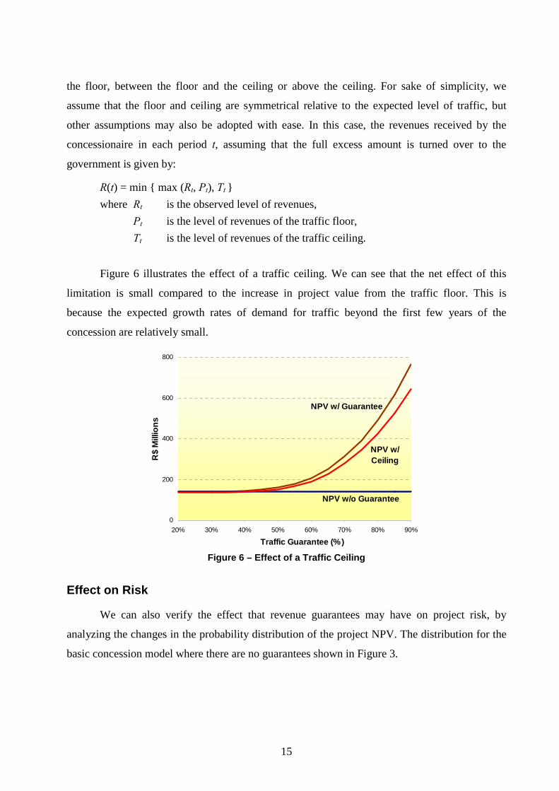
Figure 6 illustrates the effect of a traffic ceiling. We can see that the net effect of this

limitation is small compared to the increase in project value from the traffic floor. This is

because the expected growth rates of demand for traffic beyond the first few years of the

concession are relatively small.

0

200

400

600

800

20% 30% 40% 50% 60% 70% 80% 90%

Traffic Guarantee (%)

R$

Mill

ions

NPV w/o Guarantee

NPV w/ Guarantee

NPV w/ Ceiling

Figure 6 – Effect of a Traffic Ceiling

Effect on Risk

We can also verify the effect that revenue guarantees may have on project risk, by

analyzing the changes in the probability distribution of the project NPV. The distribution for the

basic concession model where there are no guarantees shown in Figure 3.

16

Project NPV

Val

ues

in 1

0^ -6

Values in Millions

0,000

0,200

0,400

0,600

0,800

1,000

1,200

1,400

1,600

Mean=139630,7

-0,75 -0,5 -0,25 0 0,25 0,5 0,75 1 1,25

1,251,25

-0,75 -0,5 -0,25 0 0,25 0,5 0,75 1 1,25

5% 90% 5% -,2863 ,6541

Mean=139630,7

Project NPV

Val

ues

in 1

0^ -6

Values in Millions

0,000

0,178

0,356

0,533

0,711

0,889

1,067

1,244

1,422

1,600

Mean=150563,9

-0,75 -0,5 -0,25 0 0,25 0,5 0,75 1 1,25

1,251,25

-0,75 -0,5 -0,25 0 0,25 0,5 0,75 1 1,25

5% 90% 5% -,2855 ,6621

Mean=150563,9

Project NPV

Val

ues

in 1

0^ -6

Values in Millions

0,000

0,178

0,356

0,533

0,711

0,889

1,067

1,244

1,422

1,600

Mean=189702,8

-0,75 -0,5 -0,25 0 0,25 0,5 0,75 1 1,25

1,251,25

-0,75 -0,5 -0,25 0 0,25 0,5 0,75 1 1,25

5% 90% 5% -,2851 ,728

Mean=189702,8

Project NPV

Val

ues

in 1

0^ -6

Values in Millions

0,000

0,178

0,356

0,533

0,711

0,889

1,067

1,244

1,422

1,600

Mean=226474,3

-0,75 -0,5 -0,25 0 0,25 0,5 0,75 1 1,25

1,251,25

-0,75 -0,5 -0,25 0 0,25 0,5 0,75 1 1,25

5% 90% 5% -,277 ,7838

Mean=226474,3

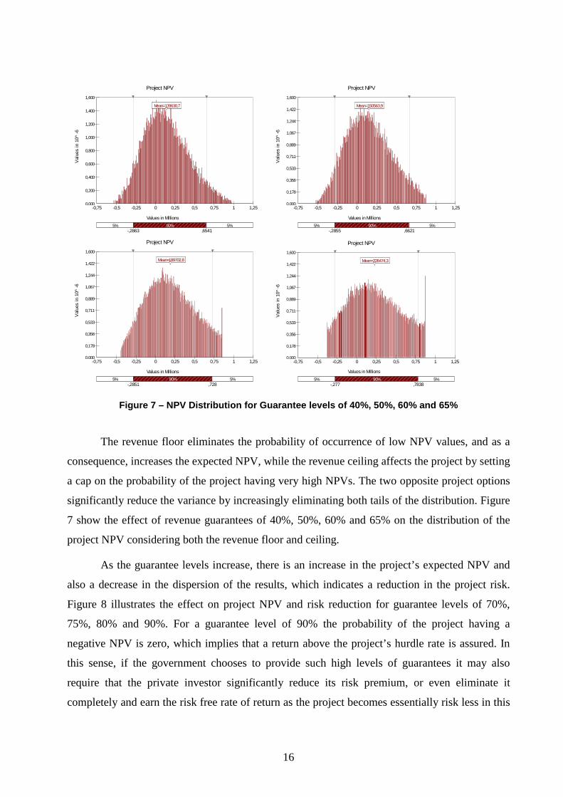
Figure 7 – NPV Distribution for Guarantee levels of 40%, 50%, 60% and 65%

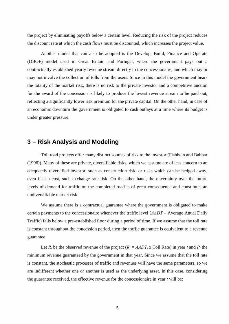
The revenue floor eliminates the probability of occurrence of low NPV values, and as a

consequence, increases the expected NPV, while the revenue ceiling affects the project by setting

a cap on the probability of the project having very high NPVs. The two opposite project options

significantly reduce the variance by increasingly eliminating both tails of the distribution. Figure

7 show the effect of revenue guarantees of 40%, 50%, 60% and 65% on the distribution of the

project NPV considering both the revenue floor and ceiling.

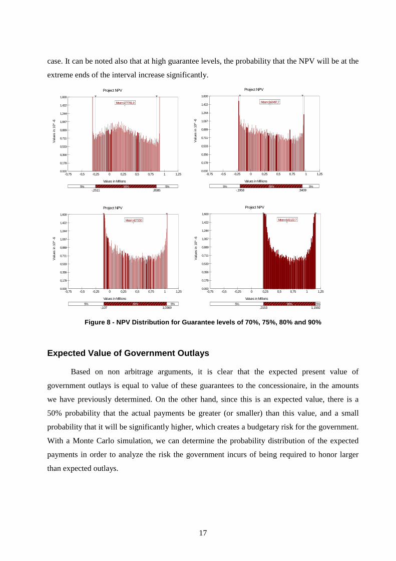
As the guarantee levels increase, there is an increase in the project’s expected NPV and

also a decrease in the dispersion of the results, which indicates a reduction in the project risk.

Figure 8 illustrates the effect on project NPV and risk reduction for guarantee levels of 70%,

75%, 80% and 90%. For a guarantee level of 90% the probability of the project having a

negative NPV is zero, which implies that a return above the project’s hurdle rate is assured. In

this sense, if the government chooses to provide such high levels of guarantees it may also

require that the private investor significantly reduce its risk premium, or even eliminate it

completely and earn the risk free rate of return as the project becomes essentially risk less in this

17

case. It can be noted also that at high guarantee levels, the probability that the NPV will be at the

extreme ends of the interval increase significantly.

Project NPV

Val

ues

in 1

0^ -6

Values in Millions

0,000

0,178

0,356

0,533

0,711

0,889

1,067

1,244

1,422

1,600

Mean=277781,9

-0,75 -0,5 -0,25 0 0,25 0,5 0,75 1 1,25

1,251,25

-0,75 -0,5 -0,25 0 0,25 0,5 0,75 1 1,25

5% 90% 5% -,2511 ,8585

Mean=277781,9

Project NPV

Valu

es in

10^

-6

Values in Millions

0,000

0,178

0,356

0,533

0,711

0,889

1,067

1,244

1,422

1,600

Mean=342497,7

-0,75 -0,5 -0,25 0 0,25 0,5 0,75 1 1,25

1,251,25

-0,75 -0,5 -0,25 0 0,25 0,5 0,75 1 1,25

5% 90% 5% -,1958 ,9409

Mean=342497,7

Project NPV

Val

ues

in 1

0^ -6

Values in Millions

0,000

0,178

0,356

0,533

0,711

0,889

1,067

1,244

1,422

1,600

Mean=427200

-0,75 -0,5 -0,25 0 0,25 0,5 0,75 1 1,25

1,251,25

-0,75 -0,5 -0,25 0 0,25 0,5 0,75 1 1,25

5% 90% 5% -,107 1,0369

Mean=427200

Project NPV

Val

ues

in 1

0^ -6

Values in Millions

0,000

0,178

0,356

0,533

0,711

0,889

1,067

1,244

1,422

1,600

Mean=641122,7

-0,75 -0,5 -0,25 0 0,25 0,5 0,75 1 1,25-0,75 -0,5 -0,25 0 0,25 0,5 0,75 1 1,25

5% 90% 5% ,2153 1,1592

Mean=641122,7

Figure 8 - NPV Distribution for Guarantee levels of 70%, 75%, 80% and 90%

Expected Value of Government Outlays

Based on non arbitrage arguments, it is clear that the expected present value of

government outlays is equal to value of these guarantees to the concessionaire, in the amounts

we have previously determined. On the other hand, since this is an expected value, there is a

50% probability that the actual payments be greater (or smaller) than this value, and a small

probability that it will be significantly higher, which creates a budgetary risk for the government.

With a Monte Carlo simulation, we can determine the probability distribution of the expected

payments in order to analyze the risk the government incurs of being required to honor larger

than expected outlays.

18

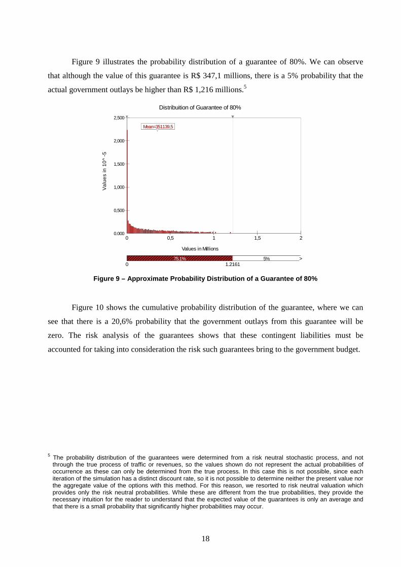
Figure 9 illustrates the probability distribution of a guarantee of 80%. We can observe

that although the value of this guarantee is R$ 347,1 millions, there is a 5% probability that the

actual government outlays be higher than R$ 1,216 millions.5

Distribuition of Guarantee of 80%

Valu

es in

10^

-5

Values in Millions

0,000

0,500

1,000

1,500

2,000

2,500

Mean=351139,5

0 0,5 1 1,5 2

00

0 0,5 1 1,5 2

75,1% 5% > 0 1,2161

Mean=351139,5

Figure 9 – Approximate Probability Distribution of a Guarantee of 80%

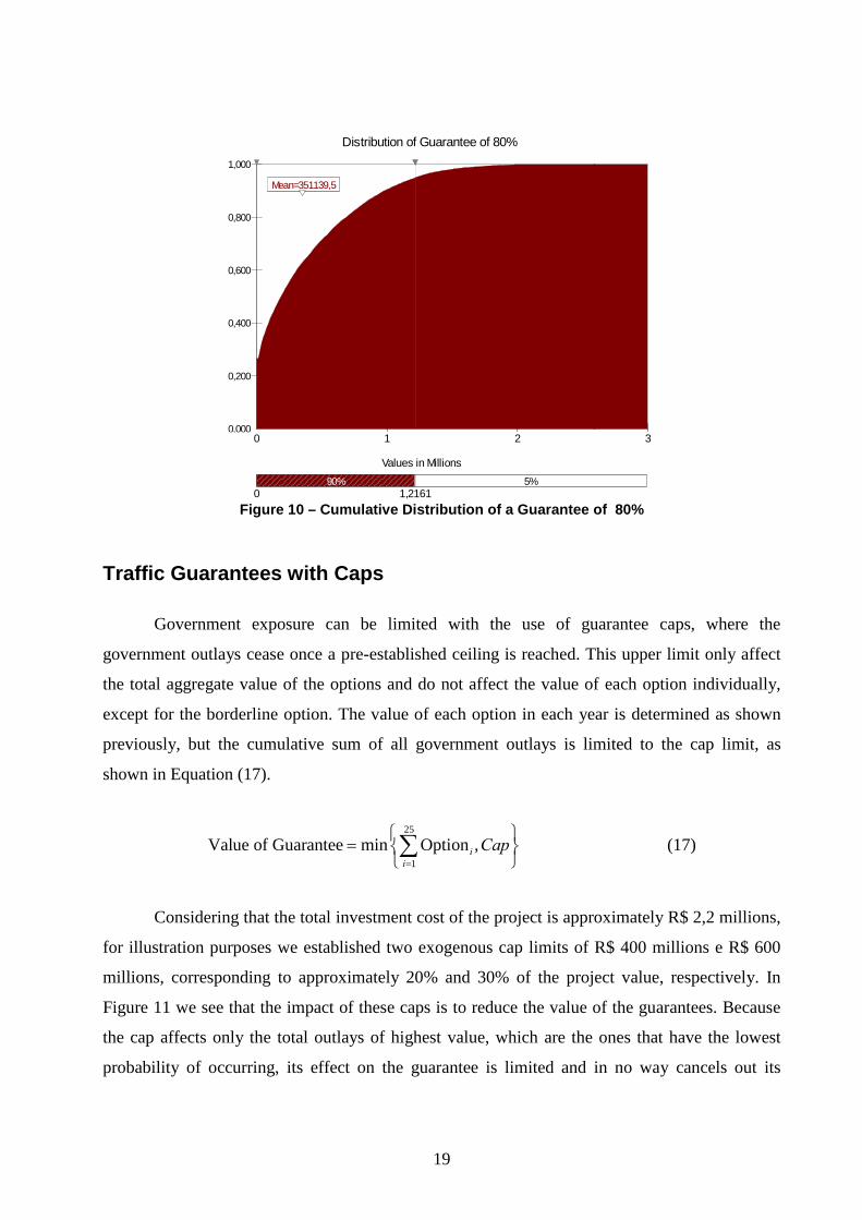
Figure 10 shows the cumulative probability distribution of the guarantee, where we can

see that there is a 20,6% probability that the government outlays from this guarantee will be

zero. The risk analysis of the guarantees shows that these contingent liabilities must be

accounted for taking into consideration the risk such guarantees bring to the government budget.

5 The probability distribution of the guarantees were determined from a risk neutral stochastic process, and not

through the true process of traffic or revenues, so the values shown do not represent the actual probabilities of occurrence as these can only be determined from the true process. In this case this is not possible, since each iteration of the simulation has a distinct discount rate, so it is not possible to determine neither the present value nor the aggregate value of the options with this method. For this reason, we resorted to risk neutral valuation which provides only the risk neutral probabilities. While these are different from the true probabilities, they provide the necessary intuition for the reader to understand that the expected value of the guarantees is only an average and that there is a small probability that significantly higher probabilities may occur.

19

Distribution of Guarantee of 80%

Values in Millions

0,000

0,200

0,400

0,600

0,800

1,000

Mean=351139,5

0 1 2 30 1 2 3

90% 5% 0 1,2161

Mean=351139,5

Figure 10 – Cumulative Distribution of a Guarantee of 80%

Traffic Guarantees with Caps

Government exposure can be limited with the use of guarantee caps, where the

government outlays cease once a pre-established ceiling is reached. This upper limit only affect

the total aggregate value of the options and do not affect the value of each option individually,

except for the borderline option. The value of each option in each year is determined as shown

previously, but the cumulative sum of all government outlays is limited to the cap limit, as

shown in Equation (17).

25

1

Value of Guarantee min Option ,ii

Cap=

⎧ ⎫= ⎨ ⎬⎩ ⎭∑ (17)

Considering that the total investment cost of the project is approximately R$ 2,2 millions,

for illustration purposes we established two exogenous cap limits of R$ 400 millions e R$ 600

millions, corresponding to approximately 20% and 30% of the project value, respectively. In

Figure 11 we see that the impact of these caps is to reduce the value of the guarantees. Because

the cap affects only the total outlays of highest value, which are the ones that have the lowest

probability of occurring, its effect on the guarantee is limited and in no way cancels out its

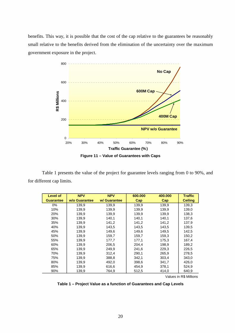
20

benefits. This way, it is possible that the cost of the cap relative to the guarantees be reasonably

small relative to the benefits derived from the elimination of the uncertainty over the maximum

government exposure in the project.

0

200

400

600

800

20% 30% 40% 50% 60% 70% 80% 90%

Traffic Guarantee (%)

R$

Mill

ions

NPV w/o Guarantee

No Cap

400M Cap

600M Cap

Figure 11 – Value of Guarantees with Caps

Table 1 presents the value of the project for guarantee levels ranging from 0 to 90%, and

for different cap limits.

Level of NPV NPV 600.000 400.000 Traffic

Guarantee w/o Guarantee w/ Guarantee Cap Cap Ceiling0% 139,9 139,9 139,9 139,9 139,3

10% 139,9 139,9 139,9 139,9 139,020% 139,9 139,9 139,9 139,9 138,330% 139,9 140,1 140,1 140,1 137,635% 139,9 141,2 141,2 141,2 137,940% 139,9 143,5 143,5 143,5 139,545% 139,9 149,6 149,6 149,5 142,550% 139,9 159,7 159,7 159,3 150,255% 139,9 177,7 177,1 175,3 167,460% 139,9 206,5 204,4 198,9 189,265% 139,9 249,9 241,6 229,3 226,570% 139,9 312,4 290,1 265,9 278,575% 139,9 388,8 342,1 303,4 343,080% 139,9 492,0 398,6 341,7 426,085% 139,9 616,6 454,9 378,1 524,990% 139,9 764,9 512,5 414,0 640,9

Values in R$ Millions Table 1 – Project Value as a function of Guarantees and Cap Levels

21

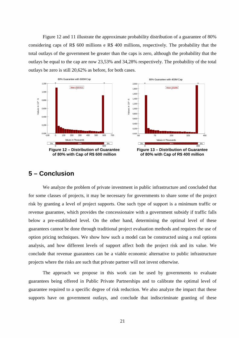
Figure 12 and 11 illustrate the approximate probability distribution of a guarantee of 80%

considering caps of R$ 600 millions e R$ 400 millions, respectively. The probability that the

total outlays of the government be greater than the caps is zero, although the probability that the

outlays be equal to the cap are now 23,53% and 34,28% respectively. The probability of the total

outlays be zero is still 20,62% as before, for both cases.

80% Guarantee with 600M Cap

Valu

es in

10^

-5

Values in Thousands

0,000

0,200

0,400

0,600

0,800

1,000

1,200

Mean=259243,5

-100 0 100 200 300 400 500 600 700-100 0 100 200 300 400 500 600 700

5% 90% 5% 0 600

Mean=259243,5

80% Guarantee with 400M Cap

Val

ues

in 1

0^ -5

Values in Thousands

0,000

0,200

0,400

0,600

0,800

1,000

1,200

1,400

1,600

1,800

2,000

Mean=201896

-50 75 200 325 450-50 75 200 325 450

5% 90% 5% 0 400

Mean=201896

Figure 12 – Distribution of Guarantee Figure 13 – Distribution of Guarantee

of 80% with Cap of R$ 600 million of 80% with Cap of R$ 400 million

5 – Conclusion

We analyze the problem of private investment in public infrastructure and concluded that

for some classes of projects, it may be necessary for governments to share some of the project

risk by granting a level of project supports. One such type of support is a minimum traffic or

revenue guarantee, which provides the concessionaire with a government subsidy if traffic falls

below a pre-established level. On the other hand, determining the optimal level of these

guarantees cannot be done through traditional project evaluation methods and requires the use of

option pricing techniques. We show how such a model can be constructed using a real options

analysis, and how different levels of support affect both the project risk and its value. We

conclude that revenue guarantees can be a viable economic alternative to public infrastructure

projects where the risks are such that private partner will not invest otherwise.

The approach we propose in this work can be used by governments to evaluate

guarantees being offered in Public Private Partnerships and to calibrate the optimal level of

guarantee required to a specific degree of risk reduction. We also analyze the impact that these

supports have on government outlays, and conclude that indiscriminate granting of these

22

guarantees can create significant future contingent liabilities for the government. We show that

the use of traffic ceilings and caps on the total outlays associated with a particular level of traffic

guarantee can help reduce this liability risk, and because they have an asymmetric impact on the

value of the project, they may be an acceptable solution to all stakeholders involved. This would

allow governments leverage their investment capabilities by redirecting scarce resources away

from financing public infrastructure investment to providing a limited level of guarantees, as

long as precautions are taken in selecting government project portfolio.

Although we analyze here only the case of a revenue guarantees, the model is flexible

and can be easily extended to include other forms of guarantees, such as shadow tolls, exchange

rate, debt and equity guarantees, and the Least Present Value of Revenues (LPVR) model

suggested by Engel, Fisher and Galetovic (2000).

23

6 - References

BEATO, P. Road Concessions: Lessons Learned from the Experience of Four Countries. Infrastructure and Financial Markets Division of the Sustainable Development Department, Inter-American Development Bank, 1997.

BLACK, F.; SCHOLES, M. The Pricing of Options and Corporate Liabilities, Journal of Political Economy, 81 (1973), 637-59.

BOUSQUET, F.; FAYARD, A. (2001), Road Infrastructure concession Practice in Europe. Policy Research Working Paper Series 2675, The World Bank.

BOWE, Michael; LEE, Ding. project evaluation in the presence of multiple embedded real options: Evidence from the Taiwan High-Speed Rail project. Journal of Asian Economics, 15 (2004) 71–98.

BRANDÃO, L. Uma aplicação da teoria das opções reais em tempo discreto para a valoração de uma concessão rodoviária. Tese de Doutorado, Pontifícia Universidade Católica do Rio de Janeiro, Rio de Janeiro, 2002.

BRANDÃO, L; DYER, J.; HAHN, W. Response to Comments on Brandão et al. Decision Analysis. Vol. 2, No. 2, June 2005, pp. 103-109.

CHAROENPORNPATTANA S.; MINATO T., NAKAHAMA S. Government Supports as bundle of Real Options in Built-Operate-Transfer Highways projects. Dissertação de Mestrado. The University of Tokyo, 2002

COPELAND, T.; ANTIKAROV, V., Real Options. Texere LLC, New York, 2001.

CROCKER, K.; S. MASTEN. Regulation and Administered Contracts Revisited: Lessons from Transaction-Cost Economics for Public Utility Regulation. Journal of Regulatory Economics 9:5-40, 1996.

DAILAMI, M.; KLEIN M. Government support to private infrastructure projects in emerging markets. In: Dealing with Public Risk in Private Infrastructure (eds Irwin, Klein, M, Perry, G. E. & Thobani, M.), pp.21-42. The World Bank, Washington D.C., 1997.

DIXITt, A., and PINDYCK, R., Investment under Uncertainty, Princeton University Press, Princeton, NJ (1994).

ENGEL, E.; FISHER, R.; GALETOVIC, A. The Chilean Infraestructure Concessions Program: Evaluation, Lessons and Prospects for the Future. Working Paper, Centro de Economia Aplicada (CEA), Departamento de Ingenieria Industrial de Chile, 2000.

FISHBEIN, G.; BABBAR, S. Private financing of toll roads. RMC Discussion Paper Series 117, the World Bank, Washington D.C,. 1996.

GÓMEZ-IBÁNEZ, J.A. Mexico´s Private Toll Road Program. Kennedy School of Government Case Program. Case C15-97-1402.0, Harvard, 1997.

HAMMAMI, M.; RUHASHYANKIKO, J. F.; YEHOUE, E. (2006). Determinants of Public-Private Partnerships in Infrastructure. IMF Working Paper, IMF Institute.

HULL, J., Options, Futures and Other Derivatives, Prentice Hall, New Jersey 2003.

24

IRWIN, T; KLEIN, M; PERRY, G; THOBANI, M. Managing Governement Exposure do Private Infrastructure Risks. The World Research Observer, vol. 14, no. 2 (August 1999), pp. 229-45. IBRD, World Bank, Washington, D.C.

IRWIN, Timothy. Public Money for Private Infrastructure: Deciding When to Offer Guarantees, Output-Based Subsidies, and Other Fiscal Support. World Bank working paper no 10. The World Bank, Washington, D.C., July 2003.

KLEIN, B.; CRAWFORD, R.; ALCHIAN, A. Vertical Integration, Appropriable Rents, and the Competitive Contracting Process , Journal of Law and Economics 21: 297-326, 1978.

LEWIS, C.; MODY, A. Risk Management Systems Infrastructure Liabilities, in Timothy Irwin, Michael Klein, Guillermo E. Perry, and Mateen Thobani, eds., Dealing with Public Risk in Private Infrastructure (Latin American and Caribbean Studies, Washington, D.C.: World Bank, 1998).

NG F.G.; BJÖRNSSON H.C., Using Real Option and Decision Analysis to Evaluate Investments In The Architecture, Construction And Engineering Industry, Construction Management and Economics, (June 2004) 22, 471–482

PERSAD K., BANSAL S., MAZUMDAR D., BOMBA M., MACHEMEHL R., Trans Texas Corridor Right of Way Royalty Payment Feasibility, Report by Center for Transportation Research, The University of Texas at Austin, 2004.

ROSE, S. Valuation of Interacting Real Options in a Toll Road Infrastructure project. The Quarterly Review of Economics and Finance, Vol 38, Special Issue, 1998, pages 711-723

SUMMERHILL, W. (1998). Market Intervention in a Backward Economy: Railway Subsidy in Brazil, 1854-1913. The Economic History Review, v. 51, n. 3, pp. 542-568.

SUMMERHILL, W. (2003). Order Against Progress Government, Foreign Investment, and Railroads in Brazil, 1854-1913. Stanford University Press.

25

Appendix I – Traffic Projections

Expected Traffic: Equivalent Vehicles

Calendar Concession Toll PlazaYear Year 1 2 3 4 5 6 7 8 9 10 11 12 132007 0 12.119 10.644 9.973 8.759 6.924 6.924 6.924 6.924 6.924 6.746 5.416 5.119 2.809 96.2052008 1 13.964 12.230 11.734 10.535 8.558 8.558 8.558 8.558 8.558 8.323 6.821 6.514 3.768 116.6802009 2 15.396 13.573 13.092 11.890 9.795 9.795 9.795 9.795 9.795 9.549 7.848 7.526 4.398 132.2462010 3 16.641 14.729 14.257 13.048 10.840 10.840 10.840 10.840 10.840 10.580 8.703 8.365 4.891 145.4112011 4 17.760 15.760 15.294 14.081 11.764 11.764 11.764 11.764 11.764 11.494 9.453 9.099 5.312 157.0712012 5 18.792 16.709 16.244 15.016 12.600 12.600 12.600 12.600 12.600 12.317 10.126 9.758 5.683 167.6442013 6 19.753 17.590 17.123 15.876 13.366 13.366 13.366 13.366 13.366 13.072 10.742 10.355 6.019 177.3592014 7 20.660 18.414 17.947 16.677 14.076 14.076 14.076 14.076 14.076 13.768 11.309 10.907 6.326 186.3882015 8 21.522 19.197 18.720 17.431 14.739 14.739 14.739 14.739 14.739 14.420 11.839 11.420 6.615 194.8602016 9 22.001 19.484 18.979 17.626 14.916 14.916 14.916 14.916 14.916 14.581 12.002 11.563 6.779 197.5932017 10 22.485 19.780 19.245 17.826 15.098 15.098 15.098 15.098 15.098 14.745 12.172 11.712 6.947 200.3992018 11 22.968 20.083 19.519 18.037 15.285 15.285 15.285 15.285 15.285 14.918 12.344 11.864 7.124 203.2802019 12 23.459 20.397 19.803 18.252 15.479 15.479 15.479 15.479 15.479 15.094 12.524 12.024 7.303 206.2502020 13 23.953 20.720 20.091 18.475 15.680 15.680 15.680 15.680 15.680 15.278 12.712 12.186 7.490 209.3022021 14 24.456 21.052 20.390 18.707 15.889 15.889 15.889 15.889 15.889 15.467 12.903 12.354 7.684 212.4582022 15 24.960 21.395 20.702 18.950 16.102 16.102 16.102 16.102 16.102 15.665 13.101 12.528 7.886 215.6952023 16 25.476 21.749 21.020 19.198 16.326 16.326 16.326 16.326 16.326 15.869 13.307 12.709 8.095 219.0522024 17 26.002 22.111 21.349 19.456 16.558 16.558 16.558 16.558 16.558 16.078 13.523 12.896 8.308 222.5132025 18 26.536 22.489 21.689 19.724 16.798 16.798 16.798 16.798 16.798 16.297 13.744 13.091 8.532 226.0902026 19 27.080 22.876 22.039 20.002 17.046 17.046 17.046 17.046 17.046 16.524 13.974 13.290 8.764 229.7802027 20 27.635 23.280 22.401 20.291 17.306 17.306 17.306 17.306 17.306 16.761 14.212 13.498 9.006 233.6152028 21 28.206 23.694 22.777 20.592 17.574 17.574 17.574 17.574 17.574 17.006 14.460 13.714 9.256 237.5772029 22 28.787 24.123 23.162 20.901 17.856 17.856 17.856 17.856 17.856 17.259 14.719 13.940 9.515 241.6852030 23 29.383 24.565 23.563 21.223 18.148 18.148 18.148 18.148 18.148 17.524 14.988 14.173 9.787 245.9432031 24 29.994 25.023 23.980 21.559 18.452 18.452 18.452 18.452 18.452 17.799 15.267 14.414 10.068 250.3632032 25 30.619 25.496 24.405 21.904 18.767 18.767 18.767 18.767 18.767 18.086 15.558 14.667 10.362 254.932

Total

26

Appendix II – Investments and Operational Expenses (R$ 1.000,00)

Acumulated Net AcumInvestment Depreciation Investment

0 2007 283.534 283.534 283.534 283.5341 2008 268.580 268.580 552.114 (11.341) 540.7732 2009 414.634 414.634 955.407 (23.005) 932.4023 2010 0 932.402 (41.539) 890.8624 2011 0 1.012 1.189 490 2.691 893.554 (42.382) 851.1725 2012 46.063 46.128 1.189 781 94.160 945.332 (42.550) 902.7826 2013 46.063 61.837 1.638 4.167 113.706 1.016.488 (47.267) 969.2217 2014 46.063 62.734 1.189 1.072 111.058 1.080.279 (53.499) 1.026.7808 2015 96.438 0 1.638 4.231 102.307 1.129.087 (60.016) 1.069.0729 2016 65.915 0 1.189 1.542 68.646 1.137.718 (66.417) 1.071.30110 2017 65.915 0 1.189 490 67.593 1.138.894 (71.107) 1.067.78711 2018 65.915 0 4.081 3.988 73.984 1.141.771 (75.926) 1.065.84412 2019 65.915 0 1.189 762 67.865 1.133.710 (81.555) 1.052.15513 2020 65.915 0 18.534 5.501 89.949 1.142.104 (87.208) 1.054.89514 2021 15.539 0 1.189 0 16.728 1.071.623 (95.175) 976.44815 2022 15.539 0 9.093 1.344 25.976 1.002.424 (97.420) 905.00316 2023 25.302 0 1.470 3.895 30.667 935.670 (100.242) 835.42817 2024 25.302 0 1.189 781 27.272 862.700 (103.963) 758.73618 2025 25.302 0 1.638 4.992 31.932 790.669 (107.837) 682.83119 2026 25.302 0 1.189 1.072 27.563 710.394 (112.953) 597.44120 2027 99.179 0 1.189 0 100.369 697.810 (118.399) 579.41121 2028 99.179 0 3.913 4.948 108.040 687.451 (139.562) 547.88922 2029 99.179 0 1.189 490 100.858 648.748 (171.863) 476.88523 2030 99.179 0 3.545 4.813 107.538 584.422 (216.249) 368.17324 2031 99.179 0 1.189 762 101.130 469.303 (292.211) 177.09225 2032 99.179 0 16.178 490 115.847 292.939 (292.939) 0

966.748 1.291.561 171.712 75.998 46.608 2.552.627 2.258.309

Vehicles TotalConcession

YearCalendar

YearInitial

InvestmentMainte- nance

Improve- ments

Equip- ments

OperationalInsurance Costs

0 20071 2008 0 15.689 5.570 1.080 8.137 30.4762 2009 2.249 15.689 5.570 1.080 8.137 32.7253 2010 4.498 15.689 6.234 1.080 8.077 35.5784 2011 7.252 33.032 11.146 1.080 7.857 60.3675 2012 9.997 33.032 11.146 1.080 7.610 62.8646 2013 12.779 33.032 11.146 1.080 7.338 65.3747 2014 12.779 33.032 11.146 1.080 7.045 65.0828 2015 12.779 33.032 11.146 1.080 6.734 64.7709 2016 12.779 33.032 11.146 1.080 6.404 64.44010 2017 12.779 33.032 11.146 1.080 6.058 64.09411 2018 12.779 33.032 11.146 1.080 5.696 63.73212 2019 12.779 33.032 11.146 1.080 5.329 63.36513 2020 12.779 33.032 11.146 1.080 4.956 62.99214 2021 12.779 33.032 11.146 1.080 4.578 62.61415 2022 12.779 33.032 11.146 1.080 4.194 62.23016 2023 12.779 33.032 11.146 1.080 3.804 61.84117 2024 12.779 33.032 11.146 1.080 3.409 61.44518 2025 12.779 33.032 11.146 1.080 3.006 61.04319 2026 12.779 33.032 11.146 1.080 2.598 60.63420 2027 12.779 33.032 11.146 1.080 2.183 60.21921 2028 12.779 33.032 11.146 1.080 1.761 59.79722 2029 12.779 33.032 11.146 1.080 1.332 59.36823 2030 12.779 33.032 11.146 1.080 895 58.93224 2031 12.779 33.032 11.146 1.080 452 58.48825 2032 12.779 33.032 11.146 1.080 8.647 66.683

279.570 773.763 262.580 27.000 126.238 1.469.152

Concession Year

Calendar Year

G&A Expenses Other Services

Conser-vation Salaries

27

Appendix III – Project Cash Flows

Free Cash Flow To Equity (R$ 1.000,00)

Concession Year 0 1 2 3 4 5 6 7 8 9 10 11 12Calendar Year 2007 2008 2009 2010 2011 2012 2013 2014 2015 2016 2017 2018 2019

Initial Investment (283.534) (268.580) (414.634) 0 0 0 0 0 0 0 0 0 0Financing 170.120 161.148 248.780

Net Investment (113.414) (107.432) (165.854) 0 0 0 0 0 0 0 0 0 0

PV of Net Investment (358.680)Toll Revenues 0 149.661 403.371 435.714 465.044 491.992 517.041 540.541 548.124 555.905 563.900 572.138

Toll Tax 0 (20.997) (56.593) (61.131) (65.246) (69.027) (72.541) (75.838) (76.902) (77.994) (79.115) (80.271)Net Revenues 0 128.664 346.778 374.583 399.798 422.966 444.500 464.703 471.222 477.912 484.784 491.867

Operating Costs 30.476 32.725 35.578 60.367 62.864 65.374 65.082 64.770 64.440 64.094 63.732 63.365Interest 15.311 29.814 52.204 52.204 48.724 45.244 41.764 38.283 34.803 31.323 27.842 24.362

Depreciation 11.341 23.005 41.539 42.382 42.550 47.267 53.499 60.016 66.417 71.107 75.926 81.555Total Costs 57.129 85.544 129.321 154.953 154.139 157.885 160.344 163.068 165.660 166.524 167.501 169.282

EBT (57.129) 43.120 217.456 219.631 245.660 265.081 284.156 301.635 305.562 311.388 317.284 322.585Tax 0 (14.661) (73.935) (74.674) (83.524) (90.128) (96.613) (102.556) (103.891) (105.872) (107.876) (109.679)

Net Earnings (57.129) 28.459 143.521 144.956 162.136 174.954 187.543 199.079 201.671 205.516 209.407 212.906

+ Depreciation 11.341 23.005 41.539 42.382 42.550 47.267 53.499 60.016 66.417 71.107 75.926 81.555 - Amortization 0 0 0 (38.670) (38.670) (38.670) (38.670) (38.670) (38.670) (38.670) (38.670) (38.670) - Maintenance 0 0 0 0 (68.980) (74.782) (81.072) (184.011) (136.348) (147.817) (160.250) (173.729)

- Improvements 0 0 0 (490) (781) (4.167) (1.072) (4.231) (1.542) (490) (3.988) (762)

FCFE (358.680) (45.787) 51.464 185.061 148.179 96.255 104.602 120.228 32.183 91.527 89.647 82.426 81.301

Discount Rate = 16% IRR = 21,9% MIRR = 17,3%

PV0 = 498.531 Investment = (358.680) NPV0 = 139.850

Free Cash Flow To Equity (R$ 1.000,00)

Concession Year 12 13 14 15 16 17 18 19 20 21 22 23 24 25Calendar Year 2019 2020 2021 2022 2023 2024 2025 2026 2027 2028 2029 2030 2031 2032

Initial Investment 0 0 0 0 0 0 0 0 0 0 0 0 0 0Financing

Net Investment 0 0 0 0 0 0 0 0 0 0 0 0 0 0

PV of Net InvestmentToll Revenues 572.138 580.604 589.357 598.338 607.650 617.252 627.173 637.409 648.047 659.037 670.434 682.246 694.507 707.182

Toll Tax (80.271) (81.459) (82.687) (83.947) (85.253) (86.600) (87.992) (89.429) (90.921) (92.463) (94.062) (95.719) (97.439) (99.218)Net Revenues 491.867 499.146 506.671 514.391 522.397 530.651 539.181 547.981 557.126 566.575 576.373 586.527 597.067 607.964

Operating Costs 63.365 62.992 62.614 62.230 61.841 61.445 61.043 60.634 60.219 59.797 59.368 58.932 58.488 66.683Interest 24.362 20.882 17.401 13.921 10.441 6.961 3.480 0 0 0 0 0 0 0

Depreciation 81.555 87.208 95.175 97.420 100.242 103.963 107.837 112.953 118.399 139.562 171.863 216.249 292.211 292.939Total Costs 169.282 171.083 175.191 173.572 172.524 172.369 172.360 173.587 178.618 199.359 231.231 275.181 350.699 359.622

EBT 322.585 328.063 331.480 340.819 349.873 358.283 366.821 374.394 378.509 367.216 345.142 311.346 246.369 248.342Tax (109.679) (111.541) (112.703) (115.878) (118.957) (121.816) (124.719) (127.294) (128.693) (124.853) (117.348) (105.858) (83.765) (84.436)

Net Earnings 212.906 216.522 218.776 224.941 230.916 236.467 242.102 247.100 249.816 242.362 227.794 205.488 162.603 163.906

+ Depreciation 81.555 87.208 95.175 97.420 100.242 103.963 107.837 112.953 118.399 139.562 171.863 216.249 292.211 292.939 - Amortization (38.670) (38.670) (38.670) (38.670) (38.670) (38.670) (38.670) 0 0 0 0 0 0 0 - Maintenance (173.729) (188.342) (48.135) (52.183) (92.117) (99.865) (108.265) (117.371) (498.776) (540.730) (586.212) (635.519) (688.974) (746.925)

- Improvements (762) (5.501) 0 (1.344) (3.895) (781) (4.992) (1.072) 0 (4.948) (490) (4.813) (762) (490)

FCFE 81.301 71.218 227.147 230.163 196.476 201.114 198.012 241.609 (130.562) (163.753) (187.045) (218.594) (234.921) (290.570)