VEHICLE SUSPENSION OPTIMIZATION FOR

STOCHASTIC INPUTS

by

KAILAS VIJAY INAMDAR

Presented to the Faculty of the Graduate School of

The University of Texas at Arlington in Partial Fulfillment

of the Requirements

for the Degree of

MASTER OF SCIENCE IN MECHANICAL ENGINEERING

THE UNIVERSITY OF TEXAS AT ARLINGTON

December 2011

|| ौी गणशाय नमः ||

iii

ACKNOWLEDGEMENTS

I am grateful to my thesis advisor Dr. D. A. Hullender for the confidence he showed in

me and helping me in exploring the area of Dynamic Systems Modeling and Simulation. He has

been a great source of inspiration and help in this thesis.

I am thankful to the University of Texas at Arlington for providing me with opportunity

and excellent facilities to excel in my graduate studies.

I would like to thank Dr. Robert Woods for his valuable guidance during my thesis and

also Dr. Kamesh Subbarao for being part of my thesis committee.

I would like to take this opportunity to thank my undergraduate professors, Prof. N. V.

Sahasrabudhe, Prof. (Dr) G. R. Gogate and M. T. Puranik for motivating me in my decision to

pursue master level studies.

I am thankful to all my friends in UTA for their encouragement and cooperation.

Finally I would like to express my gratitude to my parents my elder brother and sister-in-

law for their eternal belief in me. I would not be where I am today, if not for their support and

encouragement. I am grateful to GOD for his blessings on all of us.

November 16, 2011

iv

ABSTRACT

VEHICLE SUSPENSION OPTIMIZATION FOR

STOACHASTIC INPUTS

Kailas V. Inamdar, M.S.

The University of Texas at Arlington, 2011

Supervising Professor: David A. Hullender

In the present thesis, a simulation based numerical method has been proposed for

optimization of vehicle suspension system for stochastic inputs from random road surface

profiles. Road surfaces are classified in based upon the power spectral density functions. The

road surface is considered as a stationary stochastic process in time domain assuming constant

vehicle speed. Using Fourier transforms, it is possible to generate the road surface elevations

as a function of time.

Time domain responses of the output of the suspension system are obtained using

transfer function techniques. Optimum values of the damper constant are computed by

simulation of the Quarter Car Model for generated stochastic inputs for good road holding and

passenger ride comfort. A performance index minimization procedure is developed to find

optimum damper constant value considering mutually conflicting requirements of ride comfort

and road holding. The handling of the vehicle, cornering force, tractive force depends upon the

road holding. The road holding capacity of the vehicle changes with change in vehicle speed as

well as road roughness. A quantitative measure for deciding the road holding of the vehicle is

defined.

v

TABLE OF CONTENTS

ACKNOWLEDGEMENTS ................................................................................................................ iii ABSTRACT ..................................................................................................................................... iv LIST OF ILLUSTRATIONS.............................................................................................................. vii LIST OF TABLES ........................................................................................................................... viii Chapter Page

1. INTRODUCTION……………………………………..………..…........................................ 1

1.1 Vehicle Suspension Modeling .......................................................................... 1

1.2 Mathematical Modeling of Road Surface ......................................................... 3 1.3 Outline of Thesis .............................................................................................. 3

2. FREQUENCY RESPONSE CHARACTERISTICS OF A QUARTER CAR MODEL ...... 5

2.1 Road Holding.................................................................................................... 9

2.1.1 Effect of ratio of unsprung mass to sprung mass on road holding .............................................................................. 10 2.1.2 Effect of ratio of suspension spring stiffness to tire stiffness on road holding .......................................................... 12 2.1.3 Effect of damping ratio the shock absorber on

road holding ................................................................................... 13 2.2 Vibration Isolation ........................................................................................... 14

2.2.1 Effect of ratio of unsprung mass to sprung mass on vibration isolation ............................................................. 14 2.2.2 Effect of ratio of suspension spring stiffness to tire stiffness on vibration isolation .............................................. 15 2.2.3 Effect of damping ratio the shock absorber on vibration isolation ...................................................................... 16

2.3 Suspension Travel ......................................................................................... 17

2.3.1 Effect of ratio of unsprung mass to sprung

vi

mass on suspension travel............................................................. 17 2.3.2 Effect of ratio of suspension spring stiffness to tire stiffness on suspension travel .............................................. 18 2.3.3 Effect of damping ratio of the shock absorber on suspension travel ...................................................................... 20

3. GENERATING RANDOM ROAD INPUTS ................................................................... 21

3.1 Power spectral density (PSD) in terms of auto- correlation function ......................................................................................... 23 3.2 Road surface classification by ISO ................................................................ 23 3.3 Generating random road profile using Fourier transform ............................... 26 3.3.1 Generating road surfaces using Matlab® ....................................... 27

3.3.1 Computing PSD using Matlab® ...................................................... 28 3.3.2 Computing ‘N’ and ‘H’ for the Input to the

‘rough_road_input.m’file ....................................................... 28

4. OPTIMIZATION OF THE DAMPER CONSTANT ........................................................ 33 4.1 Optimization for road Holding ........................................................................ 33

4.1.1 Computation of transfer function for Quarter Car Model ......................................................................... 34

4.1.2 Time domain response of Quarter Car Model using Matlab® ...................................................................... 35

4.2 Optimum damper constant for minimum dynamic tire deflection ................................................................................................ 35

4.2.1 Optimization by simulation method ................................................ 35

4.2.2 Optimization by analytical method ................................................. 38

4.3 Optimization for passenger ride comfort ....................................................... 41 4.4 Performance Index minimization procedure .................................................. 44 4.5 Computation of road holding of the vehicle .................................................... 46

4.5.1 Effect of vehicle speed on road holding ......................................... 48 4.5.2 Effect of road surface on road holding ........................................... 49

5. RESULTS AND CONCLUSION ................................................................................... 53

vii

APPENDIX

A. MATLAB® FILES FOR USED FOR GENERATING STOCHASTIC INPUTS AND OUTPUT RESPONSES IN TIME DOMAIN .................................................................................................................. 55

REFERENCES ............................................................................................................................... 63 BIOGRAPHICAL INFORMATION .................................................................................................. 64

viii

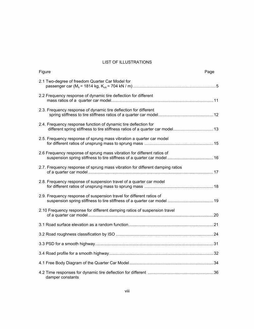
LIST OF ILLUSTRATIONS

Figure Page 2.1 Two-degree of freedom Quarter Car Model for passenger car (Ms = 1814 kg, Kus = 704 kN / m) ........................................................................ 5 2.2 Frequency response of dynamic tire deflection for different mass ratios of a quarter car model ......................................................................................... 11 2.3. Frequency response of dynamic tire deflection for different spring stiffness to tire stiffness ratios of a quarter car model ................................................ 12 2.4. Frequency response function of dynamic tire deflection for different spring stiffness to tire stiffness ratios of a quarter car model ................................... 13 2.5. Frequency response of sprung mass vibration a quarter car model for different ratios of unsprung mass to sprung mass ............................................................ 15 2.6 Frequency response of sprung mass vibration for different ratios of suspension spring stiffness to tire stiffness of a quarter car model ........................................ 16 2.7. Frequency response of sprung mass vibration for different damping ratios of a quarter car model ............................................................................................................. 17 2.8. Frequency response of suspension travel of a quarter car model for different ratios of unsprung mass to sprung mass ............................................................ 18 2.9. Frequency response of suspension travel for different ratios of suspension spring stiffness to tire stiffness of a quarter car model ........................................ 19 2.10 Frequency response for different damping ratios of suspension travel of a quarter car model ............................................................................................................. 20 3.1 Road surface elevation as a random function .......................................................................... 21 3.2 Road roughness classification by ISO ..................................................................................... 24 3.3 PSD for a smooth highway ....................................................................................................... 31 3.4 Road profile for a smooth highway ........................................................................................... 32 4.1 Free Body Diagram of the Quarter Car Model ......................................................................... 34 4.2 Time responses for dynamic tire deflection for different ......................................................... 36 damper constants

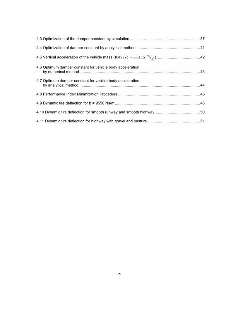
ix

4.3 Optimization of the damper constant by simulation ................................................................. 37 4.4 Optimization of damper constant by analytical method ........................................................... 41 4.5 Vertical acceleration of the vehicle mass (RMS y 0.6115 m

s ) ....................................... 42

4.6 Optimum damper constant for vehicle body acceleration by numerical method ................................................................................................................ 43 4.7 Optimum damper constant for vehicle body acceleration by analytical method ................................................................................................................ 44 4.8 Performance Index Minimization Procedure ............................................................................ 45 4.9 Dynamic tire deflection for b = 9550 Ns/m ............................................................................... 48 4.10 Dynamic tire deflection for smooth runway and smooth highway ......................................... 50 4.11 Dynamic tire deflection for highway with gravel and pasture ................................................ 51

x

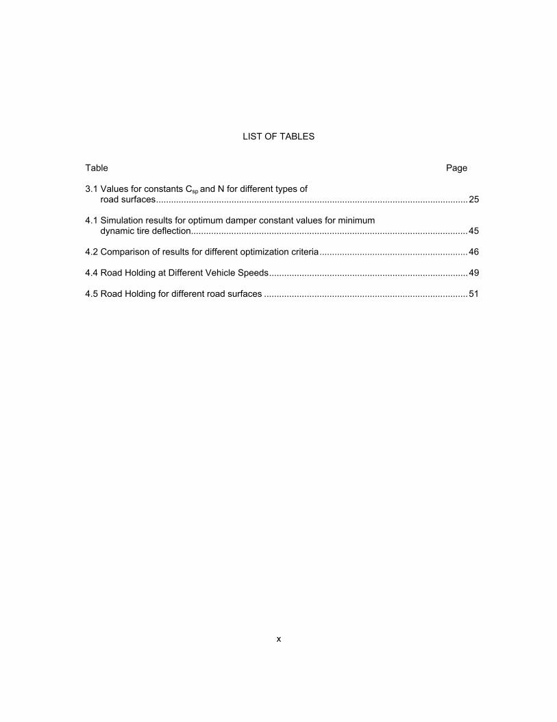
LIST OF TABLES

Table Page 3.1 Values for constants Csp and N for different types of road surfaces ............................................................................................................................ 25 4.1 Simulation results for optimum damper constant values for minimum dynamic tire deflection.............................................................................................................. 45 4.2 Comparison of results for different optimization criteria ........................................................... 46

4.4 Road Holding at Different Vehicle Speeds ............................................................................... 49

4.5 Road Holding for different road surfaces ................................................................................. 51

1

CHAPTER 1

INTRODUCTION

1. Vehicle Suspension Modeling

Modeling and simulation of the vehicle suspension system is required for predicting the

performance and assuring the proper functioning of a system before spending time and money

on producing it. A quantitative mathematical model used for the simulation, can accurately

predict the performance of the system. If the input to the system is deterministic and can be

computed by an explicit mathematical formula then, using the transfer function of the system,

the response of the system can be determined.

A vehicle suspension system is a complex vibration system having multiple degrees of

freedom [2]. The purpose of the suspension system is to isolate the vehicle body from the road

inputs. Various aspects of the dynamics associated with the vehicle put different requirements

on the components of the suspension system. Passenger ride comfort requires that the

acceleration of the sprung mass be relatively smaller whereas the lateral dynamic performance

requires good road holding which needs consistent normal force between the road and the tires.

This all has to work within the maximum allowed deflection of the suspension spring and

limitations of the dynamic tire deflection [7].

For analyzing the vibration characteristics of the vehicle, equations of motion have to be

formulated. Various models from a single degree of freedom model to a complex model having

multiple degrees of freedom have been developed for studying the suspension system

performance. However, the system is simplified by considering some dominating modes and

modal approximations. For instance, a ’Quarter Car Model’ has been extensively used to study

the dynamic behavior of the vehicle suspension system [4]. This is basically a linear lumped

mass parameter model with two degrees of freedom. This model is used to obtain a qualitative

2

insight into the performance of the suspension, in particular the effects of sprung mass and

unsprung mass, stiffness of the suspension spring and tires, damping of the shock absorbers

and tires on the vehicle vibration.

The inputs to the road surface are rough road irregularities. These irregularities range

from potholes to random variations in the surface elevations along the length of the road. These

act as a major source of excitation for the vehicle suspension system. When a vehicle traverses

over such a road surface with a certain velocity, the irregularities on the road surface become

an input with certain frequencies for the suspension system. Due to the mass imbalances and

differences in the stiffness of the suspension and wheel assembly, these excitations from the

ground are transmitted to the vehicle body. If the level of vibrations induced in the vehicle

exceeds a certain threshold then it makes the ride uncomfortable for the passenger. Secondly,

the suspension components are subjected to fluctuating loads due to these vibrations which

cause fatigue in the springs and other components of the suspension. Another significant effect

that the road excitations have is on the handling of the vehicle. If the amplitude of tire

oscillations exceeds a maximum limit then, the vehicle loses its road holding capacity and

adversely affects the handling of the vehicle.

All these effects arising from the random road irregularities can be formulated and

analyzed using a simulation based approach for design and optimization of the vehicle

suspension system [8]. The computer simulation consists of three stages. The first stage is

generation of a random input with stochastic properties and characteristics of road profiles that

the suspension system would encounter in practice. This input is used to excite the system. The

second stage deals with the numerical solution of the differential equations representing the

dynamics of the system. The numerical solution obtained by solving the differential equations,

by numerical integration method, represents the output of the system. The third stage of the

computer simulation consists of processing the output data [3].

3

1.2 Mathematical Modeling of Road Surface

The road surface is conventionally modeled in the form of step input [7], sine waves or

triangular waves with amplitude depending upon the surface elevations and the frequency

depending upon the wavelengths of the surface irregularities. However, in practice the road

surfaces are of irregular forms and the actual ride behavior of the vehicle cannot be studied

considering these forms of input. Therefore, the simplified form of inputs can be used only for

the comparative evaluation of different suspension designs [2].

To study the actual ride behavior of the vehicle and performance of the suspension

system, the road surface should be modeled as a stochastic process. In practice, the road

surface elevations are random in nature. The instantaneous value of the surface elevation at

any point above some reference plane cannot be computed by an explicit mathematical

relationship or as a function of the distance between the point of elevation and some fixed point

of reference. As a consequence of this, when a vehicle is running over the road surface, the

excitations imposed to the vehicle forms a set of random data. Therefore the road surface

should be modeled as a stochastic process. A random process is the one in which there is no

way to predict the exact value at a future instant of time [1]. However, if sufficient knowledge of

the basic mechanisms producing the random data is available then, it is possible to describe

process with exact mathematical relationships. In the following chapters we will see that by

evaluating some fix statistical properties and average values, it is possible to define a stochastic

process in deterministic manner.

1.3 Outline of Thesis

Chapter 2 discusses the frequency response characteristics of the quarter car model.

These characteristics depend upon the fixed parameters of the system such as vehicle mass,

suspension spring stiffness, shock absorber damper constant, mass and stiffness of the tires

etc. While the vehicle is moving on a road surface, the input excitations consists of large

4

number of frequencies. So it is necessary to study the frequency response characteristics of the

suspension system.

In chapter 3, procedure for generating random time series with a specified spectral

density function is explained. This used for creating road surface profiles.

Chapter 4 gives procedures for finding an optimum value of shock absorber damper

constant considering road holding and passenger ride comfort. A quantitative measure for

deciding the road holding capacity of the vehicle at different speeds and for different types of

the road surfaces is also explained in this chapter.

Chapter 5 contains results and conclusion of the simulations.

5

CHAPTER 2

FREQUENCY RESPONSE CHARACTERISTICS OF QUARTER CAR MODEL

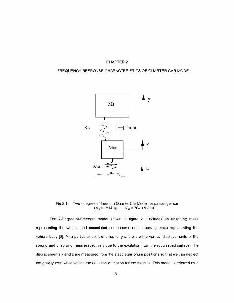
Fig 2.1. Two - degree of freedom Quarter Car Model for passenger car (Ms = 1814 kg, Kus = 704 kN / m)

The 2-Degree-of-Freedom model shown in figure 2.1 includes an unsprung mass

representing the wheels and associated components and a sprung mass representing the

vehicle body [2]. At a particular point of time, let y and z are the vertical displacements of the

sprung and unsprung mass respectively due to the excitation from the rough road surface. The

displacements y and z are measured from the static equilibrium positions so that we can neglect

the gravity term while writing the equation of motion for the masses. This model is referred as a

6

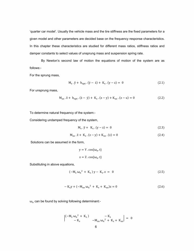
‘quarter car model’. Usually the vehicle mass and the tire stiffness are the fixed parameters for a

given model and other parameters are decided base on the frequency response characteristics.

In this chapter these characteristics are studied for different mass ratios, stiffness ratios and

damper constants to select values of unsprung mass and suspension spring rate.

By Newton’s second law of motion the equations of motion of the system are as

follows:-

For the sprung mass,

M . y b . y z K . y z 0 2.1

For unsprung mass,

M . z b . z y K . z y K . z u 0 2.2

To determine natural frequency of the system:-

Considering undamped frequency of the system,

M . y K . y z 0 2.3

M . z K . z y K . z 0 2.4

Solutions can be assumed in the form,

y Y . cos ω . t

z Z . cos ω . t

Substituting in above equations,

M ω K y K . z 0 2.5

K y M ω K K z 0 2.6

ω can be found by solving following determinant:-

M ω K K K M ω K K

0

7

ω M M ω M K M K M K K K 0 2.7

ω B B 4 A C

2 A 2.8

And

ω B B 4 A C

2 A 2.9

Where,

A M M

B M K M K M K

C K K

Substituting the values for the quarter car model shown in figure 3.1, we get,

ω 6.5626 rad sec i. e. f 1.0445 Hz

ω 66.19 rad sec i. e. f 10.53 Hz

For the passenger car, the mass of the vehicle body is much higher than the mass of

the wheel ( M M 10.02 ) while the stiffness of the suspension spring K is much less than

that of the wheel (K K 0.125). Considering this the above two natural frequencies of the

sprung and unsprung masses can be determined by an approximate method and are expressed

as follows;

Undamped natural frequency of the sprung mass,

f

2.10

f

2.11

Using these approximate formulae, the same two natural frequencies are computed as,

8

f 1.045 Hz

f 10.527 Hz

Hence these values are practically identical with the actual undamped natural frequencies of the

vehicle and wheels.

The transfer function is computed using Matlab® as follows;

HY_U 5.336 109 s 6.195 1010

328333 s4 1995 b s3 1.4526 109 s2 704000 b s 6.1925 1010

From the eigenvalues of the characteristic equation, natural frequencies can be found

>> damp(HY_U)

Eigenvalue Damping Freq. (rad/s)

-1.69e+000 + 6.46e+000i 2.54e-001 6.67e+000

-1.69e+000 - 6.46e+000i 2.54e-001 6.67e+000

-2.13e+001 + 6.15e+001i 3.28e-001 6.51e+001

-2.13e+001 - 6.15e+001i 3.28e-001 6.51e+001

The eigenvalues are 1.69 j 6.46 and 21.3 j 61.5

Natural frequencies of sprung and unsprung masses are

f 1.028 Hz

f 10.36 Hz

The frequency values calculated by equations 2.10 and 2.11 closely match with the values

computed using the transfer function using Matlab®.

Secondly, the natural frequency of the unsprung mass is higher than that of the sprung

mass. For the passenger cars, the damping ratio ( ζ) provided by the shock absorbers is usually

in the range of (0.2 – 0.4) and the damping ratio of the tires is comparatively less (~ 0.03) . As a

consequence of this, the difference between the undamped and damped natural frequencies of

the masses is negligible and the undamped natural frequencies are commonly used to

9

characterize the system. The ratio of the natural frequencies of the sprung and unsprung

masses plays an important role in deciding the vibration isolation characteristics of the vehicle

suspension. For example, consider a situation where the running vehicle hits a bump on the

road. The bump on the road can be considered as an impulse input to the suspension system.

As the vehicle crosses the bump, the wheel oscillates freely at its natural frequency which in this

case is 10.53 Hz. For the sprung mass the natural frequency is 1.045 Hz and the excitation is

the vibrations of the unsprung mass. Therefore, the ratio of frequency of excitation to the natural

frequency of sprung mass is approximately 10. From the frequency response characteristics,

when the ratio of the excitation frequency to the natural frequency is high, the gain of the

transfer function is low. So, the amplitude of vibration of the vehicle body would be very low and

good vibration isolation can be achieved.

Random road surfaces consist of a wide range of wavelengths. When the vehicle rides

over such a road surface at particular speed, the excitation to the vehicle consists of wide range

of frequencies. From the transmissibility characteristics of the vehicle, it can be observed that

the excitations due to shorter wavelengths of the road (i.e. high frequency inputs) can be

isolated effectively since the natural frequency of the sprung mass is low. However, excitations

from the larger wavelengths (i.e. the low frequency inputs) can be transmitted to the vehicle

body unimpeded or even amplified since the gain of the transfer function is high when the

frequency of excitation is close to the natural frequency of the vehicle body.

Evaluation of the overall performance of the suspension system is carried out by

considering three main aspects as follows:

1. Road holding

2. Vibration isolation

3. Suspension travel

10

2.1 Road Holding

The normal force between the road and the tire can be represented by relative

displacement between unsprung mass and the road surface elevations, which is also called as

the dynamic tire deflection. The dynamic tire deflection represents the normal force acting

between the tire and road surface consider the damping of the tires negligible.

The ratio of the relative displacement between the unsprung mass and the road surface

(z u) to the amplitude of the rough road surface is defined as the dynamic tire deflection ratio.

The cornering force, tractive effort and braking effort developed by the tire are related to the

normal force acting between the tire and the road surface. When the vehicle system vibrates,

this normal force fluctuates and as a consequence, the road holding capacity of the vehicle is

affected causing unfavorable effects on handling and performance of the vehicle. Therefore, it

becomes necessary to study the effects of different parameters on the dynamic tire deflection

ratio.

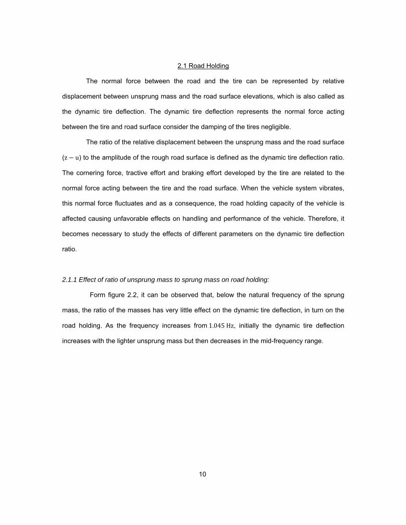
2.1.1 Effect of ratio of unsprung mass to sprung mass on road holding:

Form figure 2.2, it can be observed that, below the natural frequency of the sprung

mass, the ratio of the masses has very little effect on the dynamic tire deflection, in turn on the

road holding. As the frequency increases from 1.045 Hz, initially the dynamic tire deflection

increases with the lighter unsprung mass but then decreases in the mid-frequency range.

11

Figure 2.2 Frequency response of dynamic tire deflection for different mass ratios of a quarter car model

Above natural frequency of unsprung mass, the unsprung mass has insignificant effect on the

roadholding. Consider that the vehicle is moving with speed V , on a road surface having

wavelengths l . So, the excitation frequency for the suspension system would be f V/l Hz

If this frequency f, matches the frequency at which the positive value of dynamic tire deflection

becomes equal to the static deflection of the tire due to the vehicle weight then, the tire is on the

verge of bouncing off the ground. During this part of vibrations, the vehicle will not have any

contact with ground. Such situation is very undesirable since it reduces the handling

performance.

12

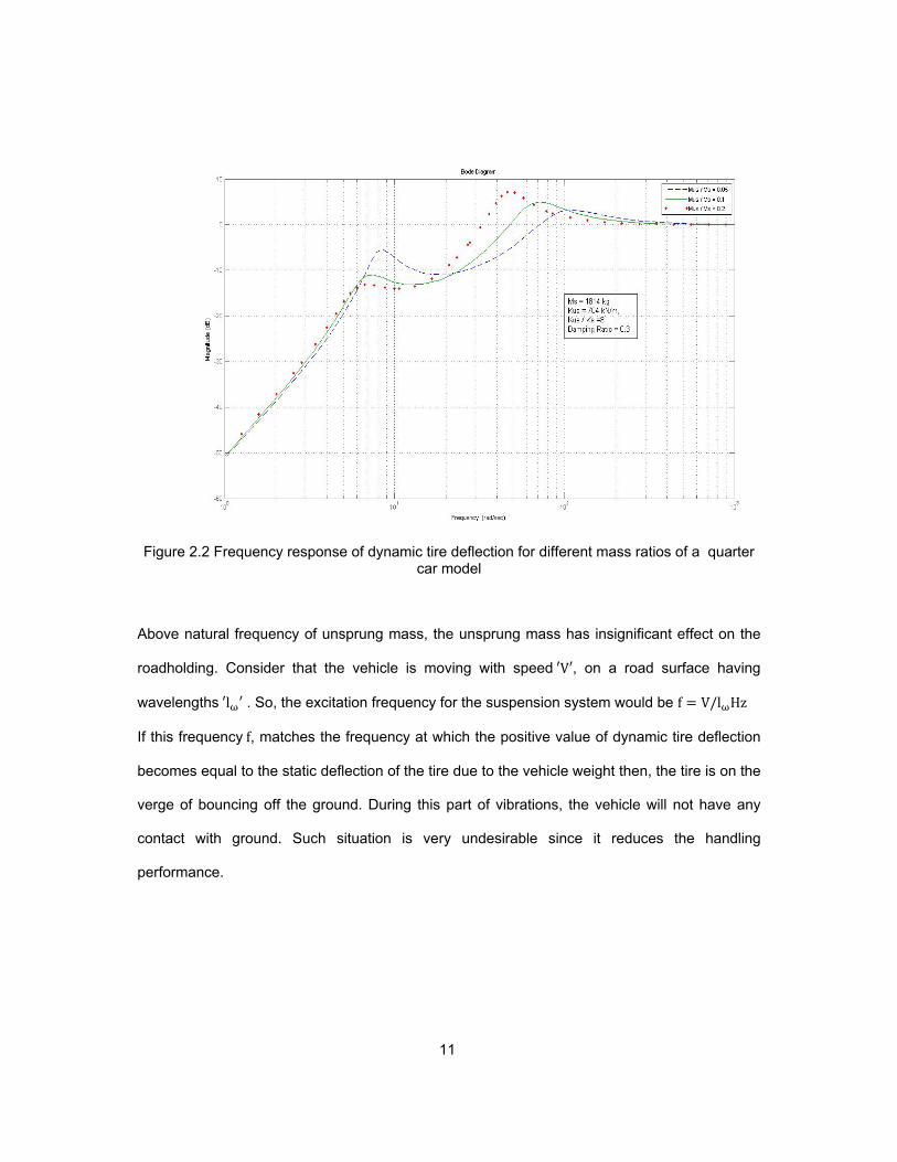
2.1.2 Effect of ratio of spring stiffness to tire stiffness on road holding:

Figure 2.3 Frequency response of dynamic tire deflection ratio for different spring stiffness to tire stiffness ratios of a quarter car model

Figure 2.3 shows that, in the low frequency range, below the natural frequency of the sprung

mass and high frequency range, above the natural frequency of the unsprung mass, the effect

of the suspension spring stiffness on the dynamic tire deflection ratio is insignificant. Between

the natural frequency of sprung mass and the crossover frequency, the dynamic tire deflection

ratio is lower with the softer suspension spring. Between the crossover frequency and the

natural frequency of the unsprung mass, a stiffer suspension spring provides lower dynamic tire

deflection ratio.

13

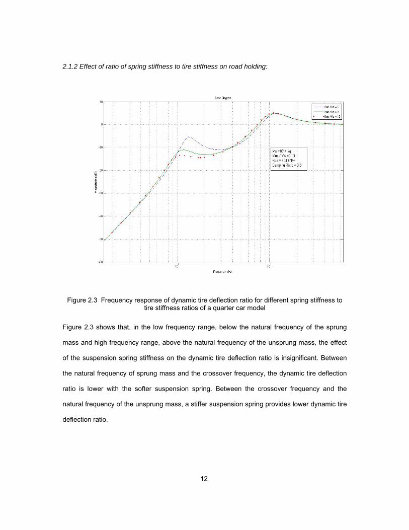
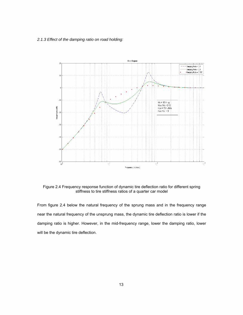
2.1.3 Effect of the damping ratio on road holding:

Figure 2.4 Frequency response function of dynamic tire deflection ratio for different spring stiffness to tire stiffness ratios of a quarter car model

From figure 2.4 below the natural frequency of the sprung mass and in the frequency range

near the natural frequency of the unsprung mass, the dynamic tire deflection ratio is lower if the

damping ratio is higher. However, in the mid-frequency range, lower the damping ratio, lower

will be the dynamic tire deflection.

14

2.2 Vibration Isolation

Vibrations in the vehicle body are usually considered as the vertical displacement of

the vehicle body due to elevations on the rough road. The vibration isolation characteristics can

be studied using the transfer function between the vehicle displacement and the road input.

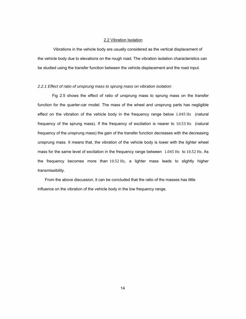
2.2.1 Effect of ratio of unsprung mass to sprung mass on vibration isolation:

Fig 2.5 shows the effect of ratio of unsprung mass to sprung mass on the transfer

function for the quarter-car model. The mass of the wheel and unsprung parts has negligible

effect on the vibration of the vehicle body in the frequency range below 1.045 Hz (natural

frequency of the sprung mass). If the frequency of excitation is nearer to 10.53 Hz (natural

frequency of the unsprung mass) the gain of the transfer function decreases with the decreasing

unsprung mass. It means that, the vibration of the vehicle body is lower with the lighter wheel

mass for the same level of excitation in the frequency range between 1.045 Hz to 10.52 Hz. As

the frequency becomes more than 10.52 Hz, a lighter mass leads to slightly higher

transmissibility.

From the above discussion, it can be concluded that the ratio of the masses has little

influence on the vibration of the vehicle body in the low frequency range.

15

Figure 2.5 Frequency response for different ratios of unsprung mass to sprung mass of a quarter car model

In the mid-frequency range, a lighter wheel assembly will provide better vibration

isolation and in the frequency range above the natural frequency of the unsprung mass, there is

a slight increase in transmissibility with the lighter wheel assembly.

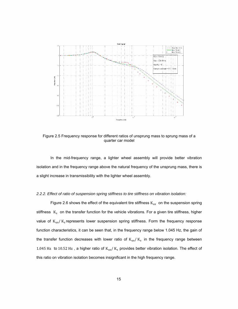
2.2.2. Effect of ratio of suspension spring stiffness to tire stiffness on vibration isolation:

Figure 2.6 shows the effect of the equivalent tire stiffness K on the suspension spring

stiffness K on the transfer function for the vehicle vibrations. For a given tire stiffness, higher

value of K / K represents lower suspension spring stiffness. Form the frequency response

function characteristics, it can be seen that, in the frequency range below 1.045 Hz, the gain of

the transfer function decreases with lower ratio of K / K in the frequency range between

1.045 Hz to 10.52 Hz , a higher ratio of K / K provides better vibration isolation. The effect of

this ratio on vibration isolation becomes insignificant in the high frequency range.

16

Figure 2.6 Frequency response for different ratios of tire stiffness to suspension spring stiffness of a quarter car model

above 10.52 Hz .

From the discussion above, it can be concluded that a softer suspension spring

provides better vibration isolation in mid- to high frequency range but with this there is some

penalty in terms of transmissibility in lower frequency range, below the natural frequency of the

sprung mass.

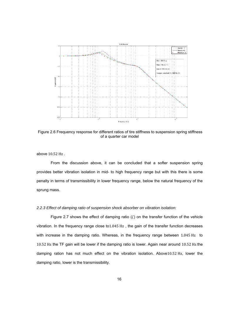
2.2.3 Effect of damping ratio of suspension shock absorber on vibration isolation:

Figure 2.7 shows the effect of damping ratio ( ) on the transfer function of the vehicle

vibration. In the frequency range close to1.045 Hz , the gain of the transfer function decreases

with increase in the damping ratio. Whereas, in the frequency range between 1.045 Hz to

10.52 Hz the TF gain will be lower if the damping ratio is lower. Again near around 10.52 Hz the

damping ration has not much effect on the vibration isolation. Above10.52 Hz, lower the

damping ratio, lower is the transmissibility.

17

Figure 2.7 Frequency response for different damping ratios of shock absorber of a quarter car model

From this it can be concluded that in the frequency range close to the natural frequency

of the vehicle body, a high damping ratio is required. However, lower damping ratio is required

to provide better vibration isolation in the mid- to high frequency range.

2.3 Suspension Travel

The relative displacement between sprung and unsprung mass is defined as the

‘suspension travel’. The space required to accommodate the spring between road bumps and

rebound stops is termed as ‘rattle space’.

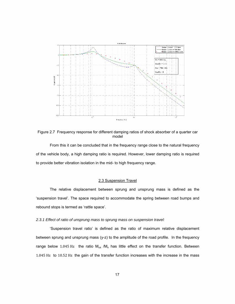
2.3.1 Effect of ratio of unsprung mass to sprung mass on suspension travel:

‘Suspension travel ratio’ is defined as the ratio of maximum relative displacement

between sprung and unsprung mass (y-z) to the amplitude of the road profile. In the frequency

range below 1.045 Hz the ratio Mus /Ms has little effect on the transfer function. Between

1.045 Hz to 10.52 Hz the gain of the transfer function increases with the increase in the mass

18

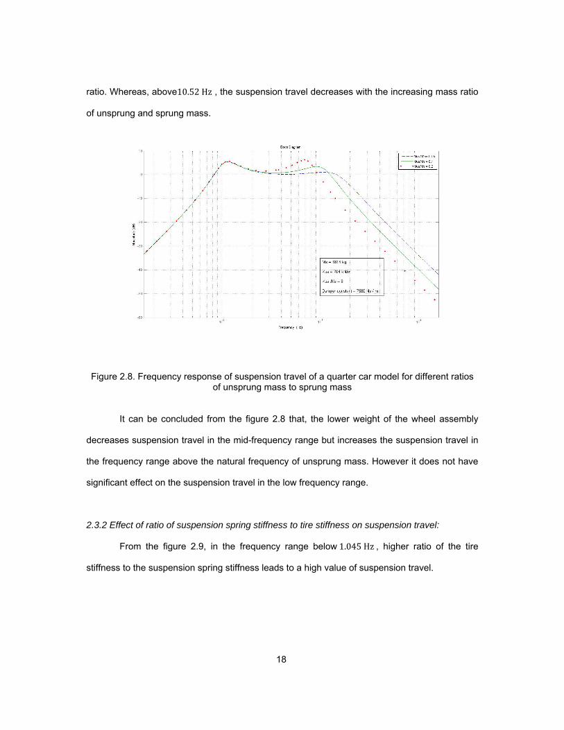
ratio. Whereas, above10.52 Hz , the suspension travel decreases with the increasing mass ratio

of unsprung and sprung mass.

Figure 2.8. Frequency response of suspension travel of a quarter car model for different ratios of unsprung mass to sprung mass

It can be concluded from the figure 2.8 that, the lower weight of the wheel assembly

decreases suspension travel in the mid-frequency range but increases the suspension travel in

the frequency range above the natural frequency of unsprung mass. However it does not have

significant effect on the suspension travel in the low frequency range.

2.3.2 Effect of ratio of suspension spring stiffness to tire stiffness on suspension travel:

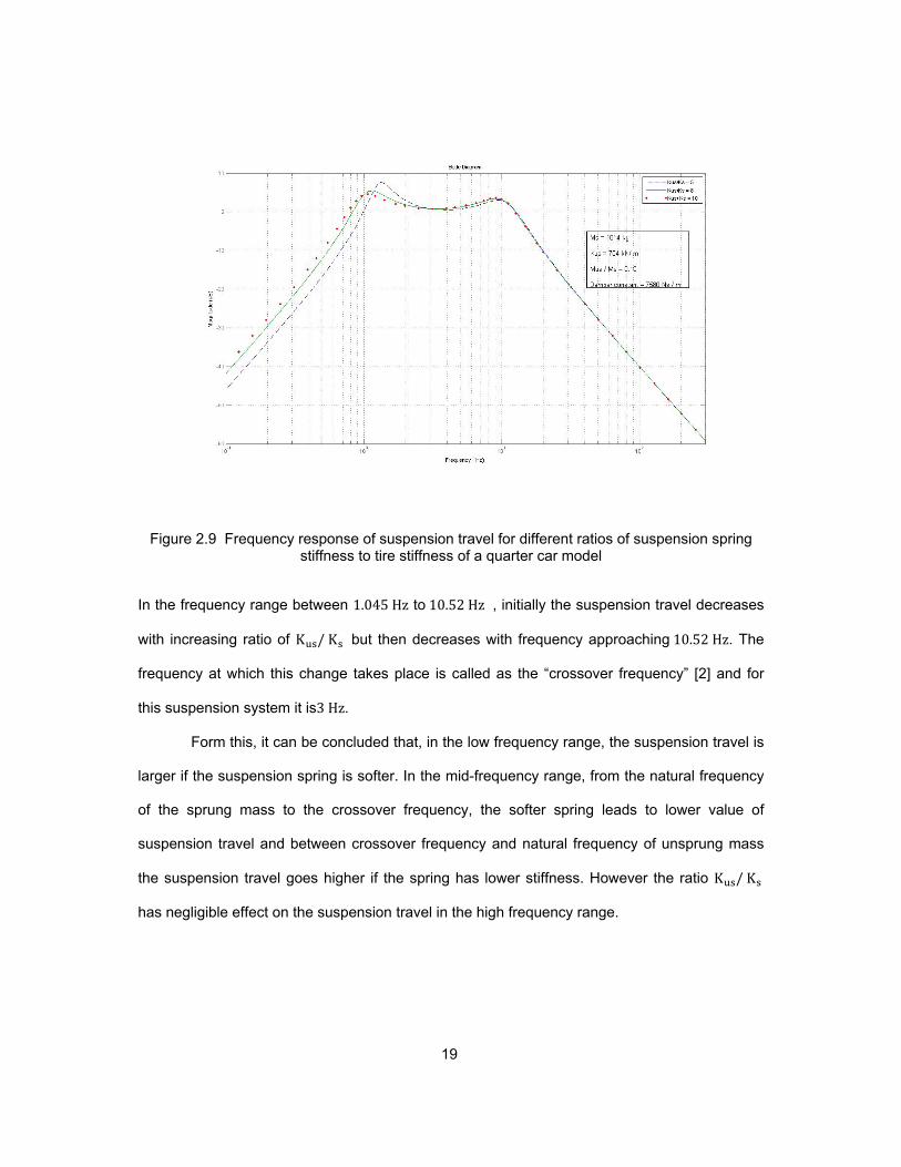
From the figure 2.9, in the frequency range below 1.045 Hz , higher ratio of the tire

stiffness to the suspension spring stiffness leads to a high value of suspension travel.

19

Figure 2.9 Frequency response of suspension travel for different ratios of suspension spring stiffness to tire stiffness of a quarter car model

In the frequency range between 1.045 Hz to 10.52 Hz , initially the suspension travel decreases

with increasing ratio of K / K but then decreases with frequency approaching 10.52 Hz. The

frequency at which this change takes place is called as the “crossover frequency” [2] and for

this suspension system it is3 Hz.

Form this, it can be concluded that, in the low frequency range, the suspension travel is

larger if the suspension spring is softer. In the mid-frequency range, from the natural frequency

of the sprung mass to the crossover frequency, the softer spring leads to lower value of

suspension travel and between crossover frequency and natural frequency of unsprung mass

the suspension travel goes higher if the spring has lower stiffness. However the ratio K / K

has negligible effect on the suspension travel in the high frequency range.

20

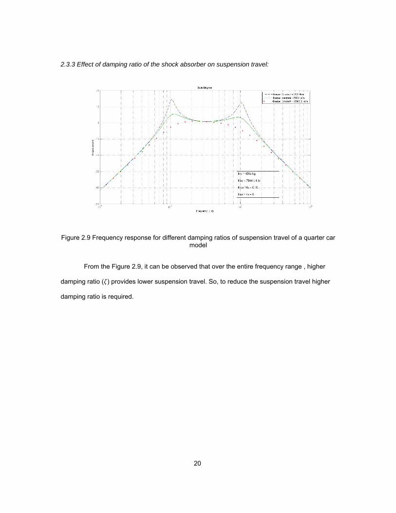
2.3.3 Effect of damping ratio of the shock absorber on suspension travel:

Figure 2.9 Frequency response for different damping ratios of suspension travel of a quarter car model

From the Figure 2.9, it can be observed that over the entire frequency range , higher

damping ratio ( ) provides lower suspension travel. So, to reduce the suspension travel higher

damping ratio is required.

21

CHAPTER 3

GENERATING RANDOM ROAD INPUTS

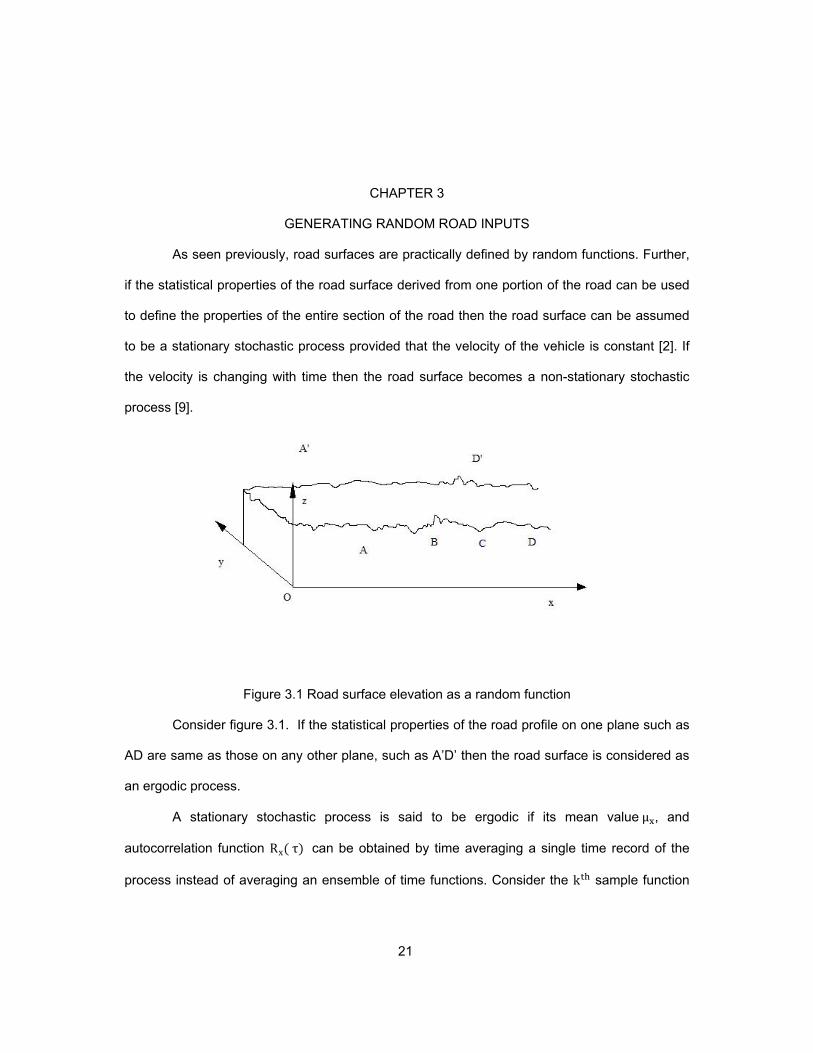
As seen previously, road surfaces are practically defined by random functions. Further,

if the statistical properties of the road surface derived from one portion of the road can be used

to define the properties of the entire section of the road then the road surface can be assumed

to be a stationary stochastic process provided that the velocity of the vehicle is constant [2]. If

the velocity is changing with time then the road surface becomes a non-stationary stochastic

process [9].

Figure 3.1 Road surface elevation as a random function

Consider figure 3.1. If the statistical properties of the road profile on one plane such as

AD are same as those on any other plane, such as A’D’ then the road surface is considered as

an ergodic process.

A stationary stochastic process is said to be ergodic if its mean value µ , and

autocorrelation function Rx τ can be obtained by time averaging a single time record of the

process instead of averaging an ensemble of time functions. Consider the k sample function

22

of the stochastic process x t . The mean value µ k and the autocorrelation function

R τ, k of the k sample function are given by,

µ k limT

1T

x t . dt

T

3.1

R τ, k limT T x t . x t τ . dt

T 3.1b

If for a stationary stochastic process, µ k and R τ, k defined in equation 3.1 do not differ

when computed over different sample functions, the stochastic process is said to be ‘ergodic’.

This assumption of the road surface being stationary ergodic process helps to simplify

mathematical modeling of the road surfaces. When a surface profile is considered as a random

function then, it can be characterized by power spectral density functions. The power spectral

density of random road surfaces is determined using digital spectral density analyzers. These

analyzers work on the principle of filtering-squaring-averaging technique. The input signal from

the road surface is passed through a highly selective narrow band pass filter with a specific

center frequency. The instantaneous value of the filtered signal is squared and an average of

this squared instantaneous value is obtained as the mean square value. The mean square

value is divided by the bandwidth to get the average power spectral density at the specific

center frequency as per equation 3.4 . By varying the center frequency of the narrow band

pass filter, power spectral densities at a series of center frequencies can be obtained and a

graph of power spectral density versus frequency can be plotted.

Consider a harmonic component un x with amplitude Un and wavelength lωn .

un x Un .sin 2 π xlωn

un x Un . sin Ωn . x 3.2

Where, Ωn - circular spatial frequency of the harmonic component

Ωn 2 π xlωn

3.3

Circular spatial frequency is expressed in rad/m

23

Let, G n Ω0 be the power spectral density at frequency nΩ0 in the frequency interval ΔΩ.

G n Ω0 . ΔΩ Un

2

2 un

2 3.4

Therefore, the discrete power spectral density becomes,

G n Ω0 U

2 . ΔΩ

uΔ Ω

3.5

3.1 Power spectral density (PSD) in terms of autocorrelation function

PSD functions are defined for frequencies ∞, ∞ and denoted by G f .

Mathematically the PSD is Fourier transform of the autocorrelation function.

G f R τ . e . dτ 3.6

Which will exist if R τ exists and if,

|R τ | ∞

The inverse Fourier transform of S f gives,

R τ G f . e . df 3.7

This relationship between the PSD and autocorrelation function is very important and

used for generating random time series with specific PSD.

3.2 Road surface classification by ISO

Various organizations have characterized the road surface roughness over the years.

The International Organization for Standardization (ISO) has proposed road roughness

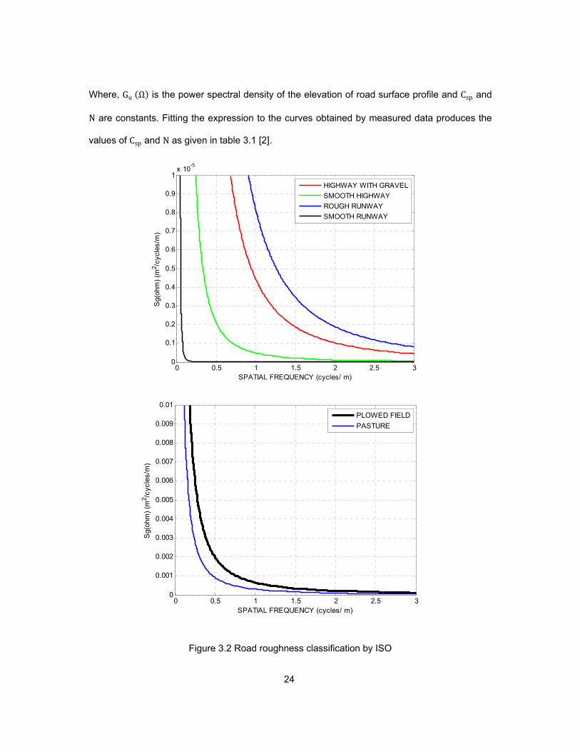
classification based on the power spectral density, as shown in Figure 3.2 [2]

The relationship between the road surface PSD and spatial frequency can be approximated as,

Gu Ω Csp . Ω‐N 3.8

24

Where, Gu Ω is the power spectral density of the elevation of road surface profile and Csp and

N are constants. Fitting the expression to the curves obtained by measured data produces the

values of Csp and N as given in table 3.1 [2].

Figure 3.2 Road roughness classification by ISO

0 0.5 1 1.5 2 2.5 30

0.001

0.002

0.003

0.004

0.005

0.006

0.007

0.008

0.009

0.01

SPATIAL FREQUENCY (cycles/ m)

Sg(

ohm

) (m

2 /cyc

les/

m)

PLOWED FIELD

PASTURE

0 0.5 1 1.5 2 2.5 30

0.1

0.2

0.3

0.4

0.5

0.6

0.7

0.8

0.9

1x 10

-5

SPATIAL FREQUENCY (cycles/ m)

Sg(

ohm

) (m

2 /cyc

les/

m)

HIGHWAY WITH GRAVEL

SMOOTH HIGHWAY

ROUGH RUNWAY

SMOOTH RUNWAY

25

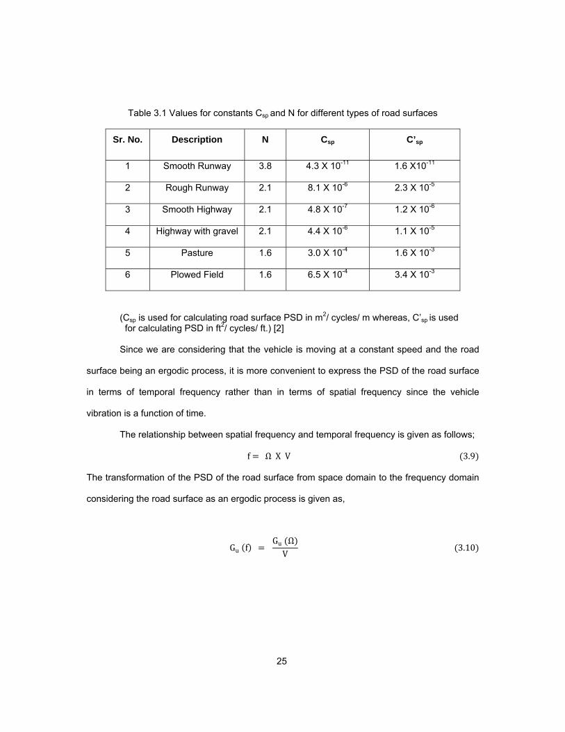
Table 3.1 Values for constants Csp and N for different types of road surfaces

Sr. No. Description N Csp C’sp

1 Smooth Runway 3.8 4.3 X 10-11 1.6 X10-11

2 Rough Runway 2.1 8.1 X 10-6 2.3 X 10-5

3 Smooth Highway 2.1 4.8 X 10-7 1.2 X 10-6

4 Highway with gravel 2.1 4.4 X 10-6 1.1 X 10-5

5 Pasture 1.6 3.0 X 10-4 1.6 X 10-3

6 Plowed Field 1.6 6.5 X 10-4 3.4 X 10-3

(Csp is used for calculating road surface PSD in m2/ cycles/ m whereas, C’sp is used for calculating PSD in ft2/ cycles/ ft.) [2] Since we are considering that the vehicle is moving at a constant speed and the road

surface being an ergodic process, it is more convenient to express the PSD of the road surface

in terms of temporal frequency rather than in terms of spatial frequency since the vehicle

vibration is a function of time.

The relationship between spatial frequency and temporal frequency is given as follows;

f Ω X V 3.9

The transformation of the PSD of the road surface from space domain to the frequency domain

considering the road surface as an ergodic process is given as,

Gu f Gu Ω

V 3.10

26

3.3 Generating random road profile using Fourier transforms

The procedure explained in the paper ‘Generation of random time series with a

specified spectral density function’ by Dr. D. A. Hullender [3] is followed for creating rough road

surfaces. By using the approach described in this paper, it is possible to generate a random

sequence of numbers which already has the desired frequency characteristics. For using this

method, the function need not be analytical and may be defined by simply a series of

frequencies at each of the values. Random road surface should be generated such that it will

have desired statistical properties. Otherwise, in evaluating the output characteristics of the

vehicle suspension, it will be impossible to completely isolate and understand the performance

characteristics of the system. In this section the procedure for this is explained. A Matlab® code

is written for generating random road profile with specific PSD.

The first step of generating a random time series of road surface elevations, u t with a

specific power spectral density, is to generate the discrete Fourier transform U f of u t based

on the desired spectral density function. By taking inverse discrete Fourier transform of U f ,

the random sequence u t is obtained. This can be done by generating random phase angles

for each of the Fourier terms of U f .

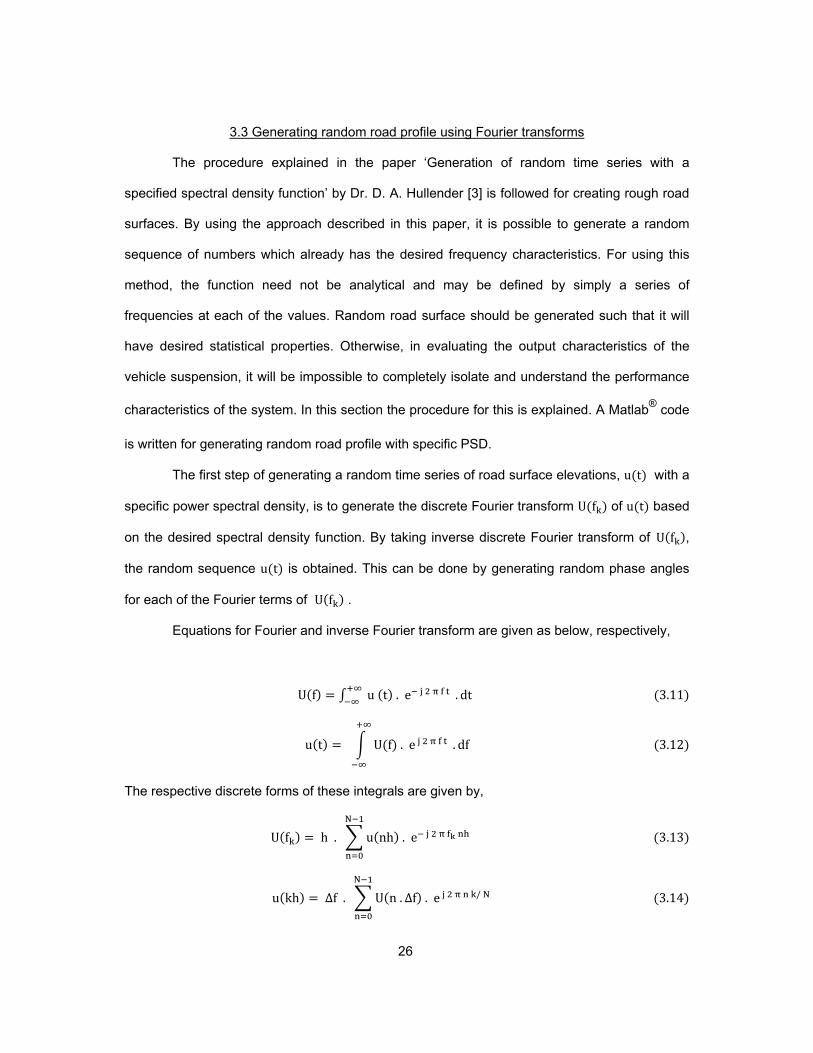
Equations for Fourier and inverse Fourier transform are given as below, respectively,

U f u t . e . dt 3.11

u t U f . e . df 3.12

The respective discrete forms of these integrals are given by,

U f h . u nh . e

N

3.13

u kh ∆f . U n . ∆f . e / N

N

3.14

27

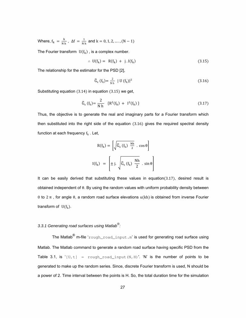
Where, f N

, ∆f N

and k 0, 1, 2, … . , N 1

The Fourier transform U f , is a complex number.

U f R f j . I f 3.15

The relationship for the estimator for the PSD [2],

Gx fk 2

N h | U fk | 3.16

Substituting equation 3.14 in equation 3.15 we get,

Gx fk 2

N h R f I f 3.17

Thus, the objective is to generate the real and imaginary parts for a Fourier transform which

then substituted into the right side of the equation 3.16 gives the required spectral density

function at each frequency fk . Let,

R f Gx fk N

. cos θ

I f j. Gx fk Nh2

. sin θ

It can be easily derived that substituting these values in equation 3.17 , desired result is

obtained independent of θ. By using the random values with uniform probability density between

0 to 2 π , for angle θ, a random road surface elevations u kh is obtained from inverse Fourier

transform of U fk .

3.3.1 Generating road surfaces using Matlab®:

The Matlab® m-file ‘rough_road_input.m’ is used for generating road surface using

Matlab. The Matlab command to generate a random road surface having specific PSD from the

Table 3.1, is ‘[U,t] = rough_road_input(N,H)'. ‘N’ is the number of points to be

generated to make up the random series. Since, discrete Fourier transform is used, N should be

a power of 2. Time interval between the points is H. So, the total duration time for the simulation

28

is NH sec and the time increment is H sec. Thus, the highest frequency generated will

be H

Hz. The frequency resolution will be 1

N H Hz.

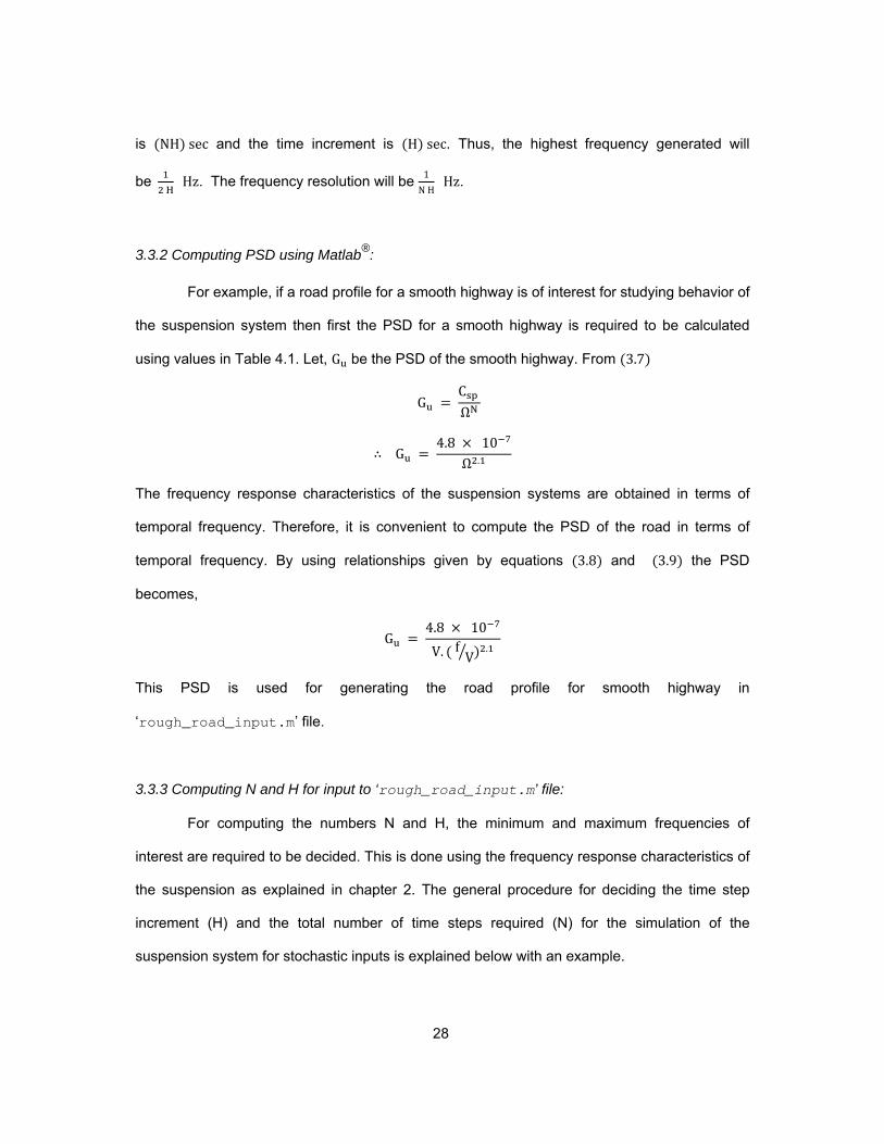
3.3.2 Computing PSD using Matlab®:

For example, if a road profile for a smooth highway is of interest for studying behavior of

the suspension system then first the PSD for a smooth highway is required to be calculated

using values in Table 4.1. Let, G be the PSD of the smooth highway. From 3.7

G C

ΩN

G 4.8 10

Ω .

The frequency response characteristics of the suspension systems are obtained in terms of

temporal frequency. Therefore, it is convenient to compute the PSD of the road in terms of

temporal frequency. By using relationships given by equations 3.8 and 3.9 the PSD

becomes,

G 4.8 10

V. f V.

This PSD is used for generating the road profile for smooth highway in

‘rough_road_input.m’ file.

3.3.3 Computing N and H for input to ‘rough_road_input.m’ file:

For computing the numbers N and H, the minimum and maximum frequencies of

interest are required to be decided. This is done using the frequency response characteristics of

the suspension as explained in chapter 2. The general procedure for deciding the time step

increment (H) and the total number of time steps required (N) for the simulation of the

suspension system for stochastic inputs is explained below with an example.

29

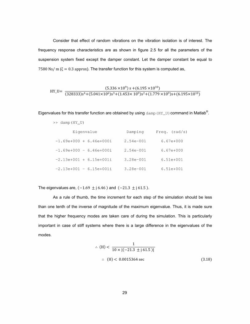
Consider that effect of random vibrations on the vibration isolation is of interest. The

frequency response characteristics are as shown in figure 2.5 for all the parameters of the

suspension system fixed except the damper constant. Let the damper constant be equal to

7580 Ns/ m (ζ 0.3 approx). The transfer function for this system is computed as,

HY_U 5.336 109 s 6.195 1010

328333 s4 5.041 106 s3 1.453 109 s2 1.779 109 s 6.195 1010

Eigenvalues for this transfer function are obtained by using damp(HY_U)command in Matlab®.

>> damp(HY_U)

Eigenvalue Damping Freq. (rad/s)

-1.69e+000 + 6.46e+000i 2.54e-001 6.67e+000

-1.69e+000 - 6.46e+000i 2.54e-001 6.67e+000

-2.13e+001 + 6.15e+001i 3.28e-001 6.51e+001

-2.13e+001 - 6.15e+001i 3.28e-001 6.51e+001

The eigenvalues are, 1.69 j 6.46 and 21.3 j 61.5 .

As a rule of thumb, the time increment for each step of the simulation should be less

than one tenth of the inverse of magnitude of the maximum eigenvalue. Thus, it is made sure

that the higher frequency modes are taken care of during the simulation. This is particularly

important in case of stiff systems where there is a large difference in the eigenvalues of the

modes.

H 1

10 | 21.3 j 61.5 |

H 0.0015364 sec 3.18

30

Secondly, the simulation should run at least for time duration equal to 5 times the

maximum value of the time constant to get the steady state response. From the eigenvalues,

the time constants are calculated as,

τ1 1r1

0.5917 sec

τ2 1r2

0.0469 sec

N H 5 τ1 i.e.

N H 2.9585 sec 3.19

Discrete Fourier transform is used in the algorithm for generating random time series with

specific spectral density, it is necessary that N is in terms of 2n where, n is a positive integer.

Using the relationships in 3.17 and 3.18 and the necessary condition for N, N and H are

calculated as follows;

N 2048 and H 0.0015 sec

Total time of simulation N H 3.072 sec

And, Frequency resolution 1

N H 0.3255 Hz

First natural frequency of the system is 1.69 Hz. With frequency resolution of 0.3255 Hz,

we would get maximum 5 points in between the minimum generated frequency and first natural

frequency of the system. Therefore the frequency resolution needs to be less. Let the frequency

resolution be less than 0.05 Hz so that there are more than 25 points between the minimum

generated frequency and the first natural frequency.

1

N H 0.05 Hz

N 1.3333 10

N 2 16384

31

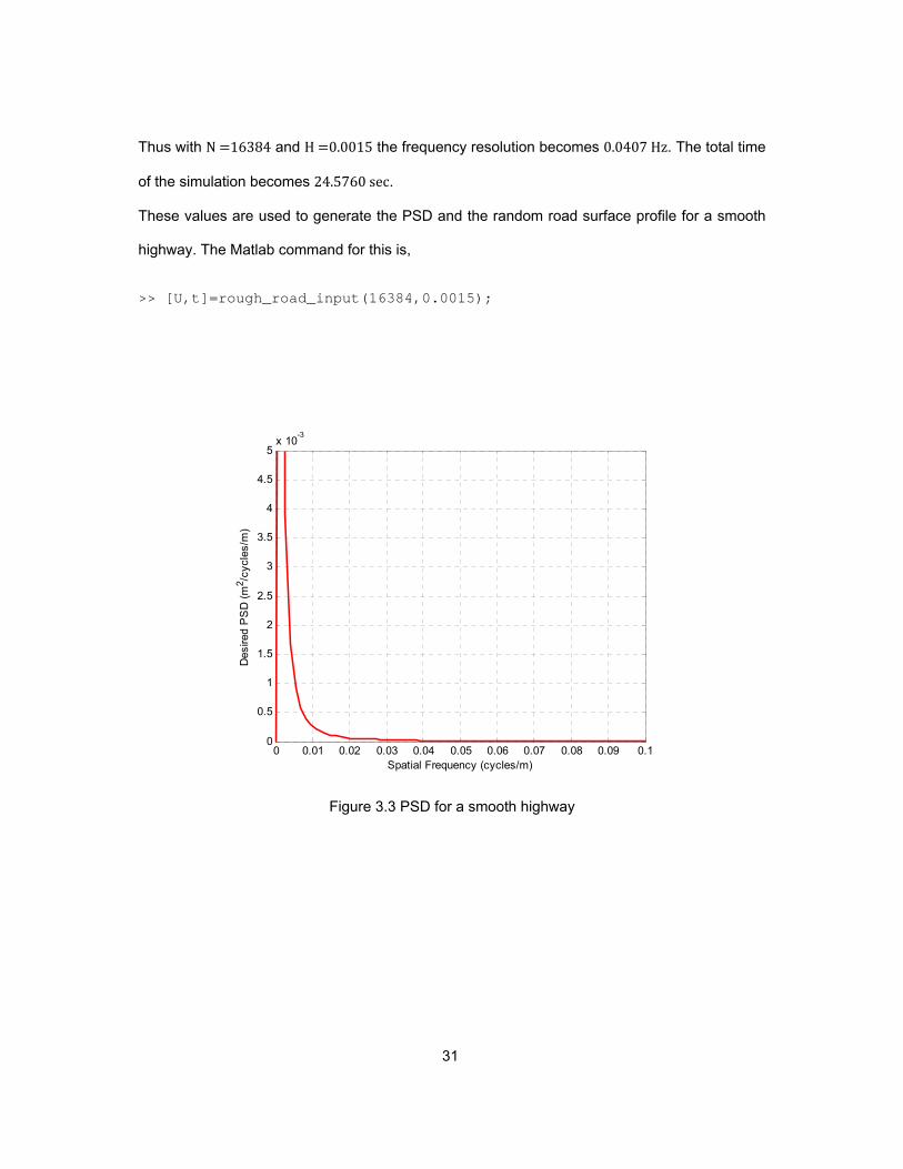
Thus with N 16384 and H 0.0015 the frequency resolution becomes 0.0407 Hz. The total time

of the simulation becomes 24.5760 sec.

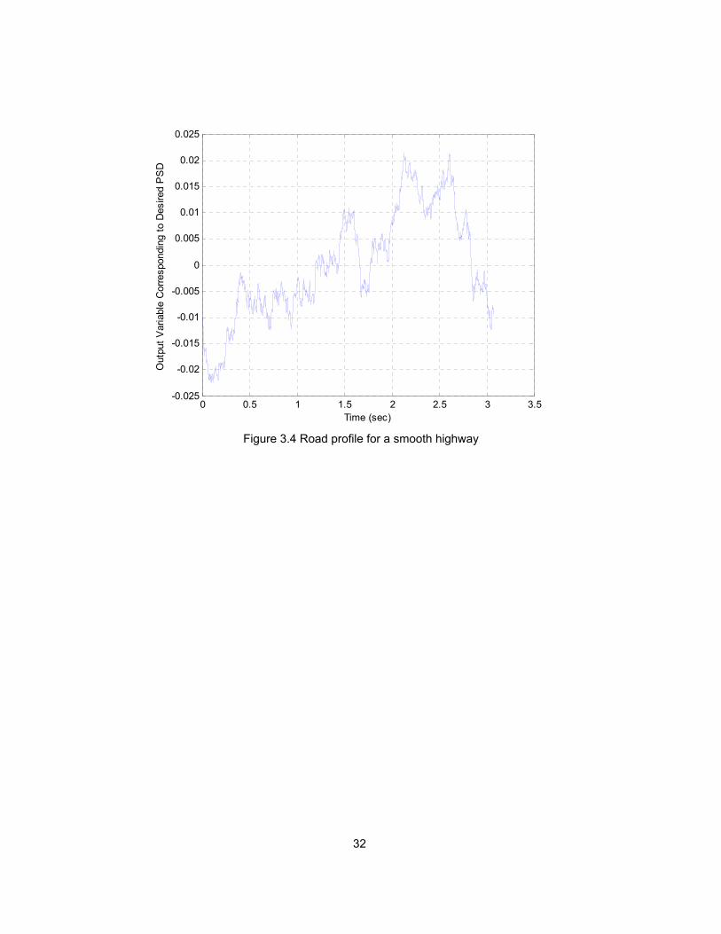
These values are used to generate the PSD and the random road surface profile for a smooth

highway. The Matlab command for this is,

>> [U,t]=rough_road_input(16384,0.0015);

Figure 3.3 PSD for a smooth highway

0 0.01 0.02 0.03 0.04 0.05 0.06 0.07 0.08 0.09 0.10

0.5

1

1.5

2

2.5

3

3.5

4

4.5

5x 10

-3

Spatial Frequency (cycles/m)

Des

ired

PS

D (

m2 /c

ycle

s/m

)

32

Figure 3.4 Road profile for a smooth highway

0 0.5 1 1.5 2 2.5 3 3.5-0.025

-0.02

-0.015

-0.01

-0.005

0

0.005

0.01

0.015

0.02

0.025

Time (sec)

Out

put

Var

iabl

e C

orre

spon

ding

to

Des

ired

PS

D

33

CHAPTER 4

OPTIMIZATION OF DAMPER CONSTANT

The performance characteristics which are of most interest while designing a vehicle

suspension system are ride comfort, road holding and suspension travel [6]. Among the three

characteristics, road holding and ride comfort are chosen for this study. All the suspension

system parameters such as sprung mass, unsprung mass, suspension spring stiffness and tire

stiffness are fixed depending upon the frequency response characteristics of the quarter car

model as explained in chapter 2. So, the damper constant of the shock absorber is selected for

optimization.

4.1 Optimization for road holding

Because of the vibrations in the vehicle suspension system while moving on a road

surface, normal force between road and the tire fluctuates. This normal force is responsible for

the road holding capacity of the vehicle. The tractive effort, braking effort and cornering force

also depends upon the normal force between the road and tires. Therefore it necessary to

maintain a minimum value of tire force for better handling of the vehicle.

Since the damping ratio of the tire is very small compared to the damping ratio of the

suspension system, it can be assumed that the normal force between the road and tire is

directly proportional to the relative displacement between the two. Mathematically, for the

quarter car model,

F K . z y 4.1

Therefore, it is possible to evaluate the road holding of the vehicle using the dynamic tire

deflection, z y . The values of the fixed parameters for the quarter car model are considered

as shown in figure 2.1. Ratio of unsprung mass to sprung mass is considered as 0.1. Ratio of

34

tire stiffness to suspension spring stiffness is considered as 8. The values of these ratios are

taken from the frequency response characteristics explained in chapter 2.

4.1.1 Computation of transfer function for the Quarter Car Model:

Matlab® is used for computing the dynamic tire deflection of the quarter-car model for

different types of road surfaces given by table 3.1. First the equations of motions are derived for

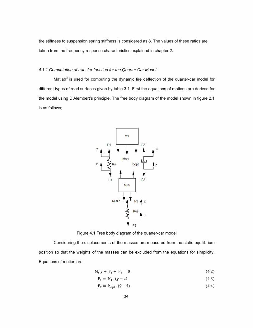
the model using D’Alembert’s principle. The free body diagram of the model shown in figure 2.1

is as follows;

Figure 4.1 Free body diagram of the quarter-car model

Considering the displacements of the masses are measured from the static equilibrium

position so that the weights of the masses can be excluded from the equations for simplicity.

Equations of motion are

M y F F 0 4.2

F K . y z 4.3

F b . y z 4.4

35

M z F F F 0 4.5

F K . z u 4.6

dtr z u 4.7

Thus 6 equations are available for finding 6 unknowns namely y, F1, F2, F3, z and dtr

By taking Laplace transform of above equations and using Matlab®, the transfer

function between road elevations u and the dynamic tire deflection dtr is obtained as follows;

Hdtr_U ‐ 328333 s4 1995 b s3 1.7556 108 s2

328333 s4 1995 b s3 1.4526 109 s2 704000 b s 6.1925 1010

4.1.2 Time domain response of the quarter car model using Matlab®:

The time response of linear time invariant models for arbitrary inputs can be obtained

using the Matlab command ’lsim(SYS_TF,U,t)’. Where, SYS_TF is the transfer function of

the system, U is the generated input and t is the time vector having same dimensions as those

og the generated input matrix U.

4.2 Optimum damper constant for minimum dynamic tire deflection

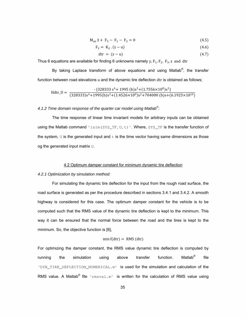
4.2.1 Optimization by simulation method:

For simulating the dynamic tire deflection for the input from the rough road surface, the

road surface is generated as per the procedure described in sections 3.4.1 and 3.4.2. A smooth

highway is considered for this case. The optimum damper constant for the vehicle is to be

computed such that the RMS value of the dynamic tire deflection is kept to the minimum. This

way it can be ensured that the normal force between the road and the tires is kept to the

minimum. So, the objective function is [6],

min f dtr RMS dtr

For optimizing the damper constant, the RMS value dynamic tire deflection is computed by

running the simulation using above transfer function. Matlab® file

‘DYN_TIRE_DEFLECTION_NUMERICAL.m’ is used for the simulation and calculation of the

RMS value. A Matlab® file ‘rmsval.m’ is written for the calculation of RMS value using

36

equation 2.2. The damper constant is varied with a step of 450 Ns/ m from 5050 Ns/ m to 12700

Ns/ m and for each value the RMS dynamic tire deflection is computed. Following figure

illustrates some of the time history records of the output for the tire deflection for the smooth

highway.

Dynamic tire deflection for b = 5050 Ns/ m RMS (dtr) = 5.2 mm

Dynamic tire deflection for b = 8200 Ns/ m

RMS (dtr) = 2.9 mm

Dynamic tire deflection for b = 10000 Ns/ m RMS (dtr) = 2.4 mm

Dynamic tire deflection for b = 12700 Ns/ m

RMS (dtr) = 3.4 mm

Figure 4.2 Time responses for dynamic tire deflection for different damper constants

0 5 10 15 20 25-0.015

-0.01

-0.005

0

0.005

0.01

0 5 10 15 20 25-10

-8

-6

-4

-2

0

2

4

6

8x 10

-3

0 5 10 15 20 25-8

-6

-4

-2

0

2

4

6

8

10x 10

-3

0 5 10 15 20 25-0.01

-0.008

-0.006

-0.004

-0.002

0

0.002

0.004

0.006

0.008

0.01

37

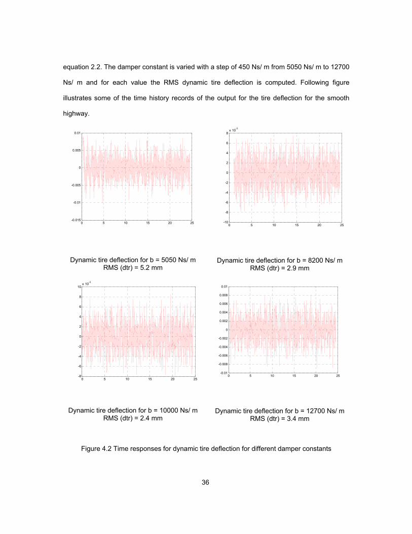
To find the optimum value of the damper constant such that the minimum dynamic tire

deflection, a graph of the tire deflection versus the damper constant is plotted.

Figure 4.3 Optimization of the damper constant by simulation

From the graph in the figure 4.3, the minimum RMS value of the dynamic tire deflection

occurs at the damper constant of the shock absorber equal to 10000 Ns/ m.

Simulations are run number of times to observe the change in minimum value of RMS

dynamic tire deflection and optimum damper constant for a smooth highway. Table 4.1 contains

the results obtained from the simulation.

From the table, it can be concluded that the value of the optimum damper constant

changes depending upon the RMS dynamic tire deflection when the vehicle is running over a

smooth highway with a constant speed. Further, simulation results are obtained for different

types of the road surfaces to find out the damper constant required for keeping the dynamic tire

2000 3000 4000 5000 6000 7000 8000 9000 10000 11000 12000 130000

0.5

1

1.5

2

2.5

3

3.5

4

4.5

5

X: 1e+004Y: 2.384

DAMPER CONSTANT (b-opt)

DY

NA

MIC

TIR

E D

EF

LEC

TIO

N B

Y S

IMU

LAT

ION

(mm

)

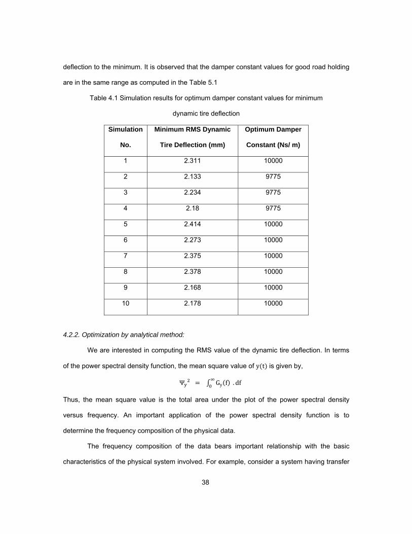
38

deflection to the minimum. It is observed that the damper constant values for good road holding

are in the same range as computed in the Table 5.1

Table 4.1 Simulation results for optimum damper constant values for minimum

dynamic tire deflection

Simulation

No.

Minimum RMS Dynamic

Tire Deflection (mm)

Optimum Damper

Constant (Ns/ m)

1 2.311 10000

2 2.133 9775

3 2.234 9775

4 2.18 9775

5 2.414 10000

6 2.273 10000

7 2.375 10000

8 2.378 10000

9 2.168 10000

10 2.178 10000

4.2.2. Optimization by analytical method:

We are interested in computing the RMS value of the dynamic tire deflection. In terms

of the power spectral density function, the mean square value of y t is given by,

Ψ Gy f . df

Thus, the mean square value is the total area under the plot of the power spectral density

versus frequency. An important application of the power spectral density function is to

determine the frequency composition of the physical data.

The frequency composition of the data bears important relationship with the basic

characteristics of the physical system involved. For example, consider a system having transfer

39

function H f . Let Gu f be the power spectral density of the input stationary random signal to

this system and Gy f be the power spectral density of the output of interest. The relationship

between these is given as [9],

Gy f |H f |2 Gu f

Let,

GU - Input PSD of the road surface

Hdtr_U - Transfer function for the dynamic tire deflection

Gd – Output PSD of dynamic tire deflection

Using above results , the output PSD of the dynamic tire deflection can be expressed as,

Gd s Hdtr_U s Hdtr_U s GU s 4.8

E dtr t - mean square value of the dynamic tire deflection,

E dtr t 1

2 π jGd s . ds 4.9

Substituting equation 4.8 into equation 4.9 ,

E dtr t 1

2 π jHdtr_U s Hdtr_U s GU s . ds

Substituting s 2 π j f and using the frequency limits as, f 0.5 Hz and f 300 Hz

The PSD of the road surface is given by,

GU C

ΩN

Where,

C 4.8 10

N 2.1 …. For smooth highway

40

Ω fV

V 30 m/sec

With these values, the road surface PSD is comes out to be,

GU f 2.0234 10

f .

For solving the integration analytically, the road PSD function is approximated as,

GU f 2.0234 10

f 4.10

The transfer function for the dynamic tire deflection is,

Hdtr_U ‐ 328333 s4 1995 b s3 1.7556 108 s2

328333 s4 1995 b s3 1.4526 109 s2 704000 b s 6.1925 1010 4.11

Where, b b (damper constant of the shock absorber to be optimized)

Substituting equation 4.10 and 4.11 in equation 4.8 , we get the output PSD for the

dynamic tire deflection. Then by substituting this value in equation 4.8 , the mean square value

can be obtained.

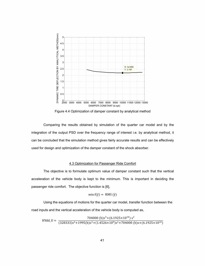
The integration is solved using Matlab® symbolic math. ‘DYNAMIC_TIRE

_DEFLECTION_ANALYTICAL.m’ file is used to plot the dynamic tire deflection against the

damping ratio. From the graph the optimum value of the damper constant can be found as

10000 Ns/ m.

41

Figure 4.4 Optimization of damper constant by analytical method

Comparing the results obtained by simulation of the quarter car model and by the

integration of the output PSD over the frequency range of interest i.e. by analytical method, it

can be concluded that the simulation method gives fairly accurate results and can be effectively

used for design and optimization of the damper constant of the shock absorber.

4.3 Optimization for Passenger Ride Comfort

The objective is to formulate optimum value of damper constant such that the vertical

acceleration of the vehicle body is kept to the minimum. This is important in deciding the

passenger ride comfort. The objective function is [6],

min f y RMS y

Using the equations of motions for the quarter car model, transfer function between the

road inputs and the vertical acceleration of the vehicle body is computed as,

HYdd_U 704000 b s3 6.1925 1010 s2

328333 s4 1995 b s3 1.4526 109 s2 704000 b s 6.1925 1010

2000 3000 4000 5000 6000 7000 8000 9000 10000 11000 12000 130000

0.5

1

1.5

2

2.5

3

3.5

4

4.5

5

X: 1e+004Y: 2.187

DAMPER CONSTANT (b-opt)

DY

NA

MIC

TIR

E D

EF

LEC

TIO

N B

Y A

NA

LYT

ICA

L M

ET

HO

D(m

m)

42

Eigenvalues of the transfer function are calculated using ’damp(HYddm_U)’

command in Matlab®. Eigenvalues are;

>> damp(HYddm_U)

Eigenvalue Damping Freq. (rad/s)

-3.02e+000 + 6.22e+000i 4.37e-001 6.91e+000

-3.02e+000 - 6.22e+000i 4.37e-001 6.91e+000

-3.56e+001 + 5.18e+001i 5.66e-001 6.28e+001

-3.56e+001 - 5.18e+001i 5.66e-001 6.28e+001

The eigenvalues are, 3.02 j 6.22 and 35.6 j 51.8

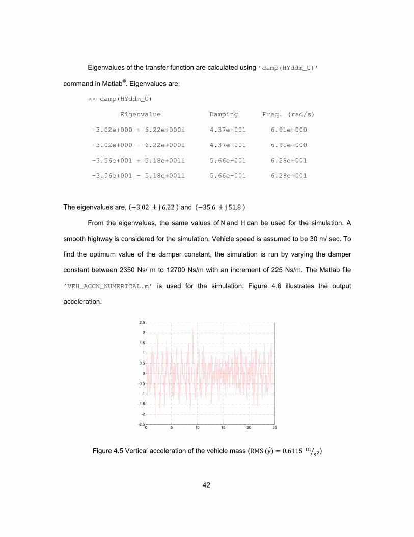
From the eigenvalues, the same values of N and H can be used for the simulation. A

smooth highway is considered for the simulation. Vehicle speed is assumed to be 30 m/ sec. To

find the optimum value of the damper constant, the simulation is run by varying the damper

constant between 2350 Ns/ m to 12700 Ns/m with an increment of 225 Ns/m. The Matlab file

’VEH_ACCN_NUMERICAL.m’ is used for the simulation. Figure 4.6 illustrates the output

acceleration.

Figure 4.5 Vertical acceleration of the vehicle mass (RMS y 0.6115 ms )

0 5 10 15 20 25-2.5

-2

-1.5

-1

-0.5

0

0.5

1

1.5

2

2.5

43

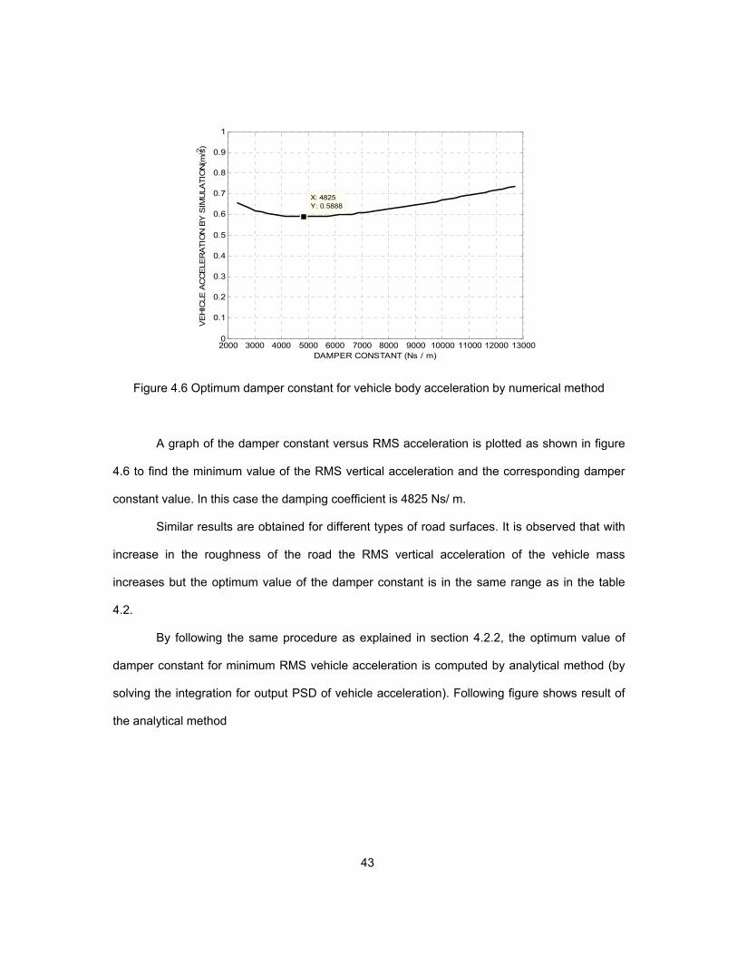
Figure 4.6 Optimum damper constant for vehicle body acceleration by numerical method

A graph of the damper constant versus RMS acceleration is plotted as shown in figure

4.6 to find the minimum value of the RMS vertical acceleration and the corresponding damper

constant value. In this case the damping coefficient is 4825 Ns/ m.

Similar results are obtained for different types of road surfaces. It is observed that with

increase in the roughness of the road the RMS vertical acceleration of the vehicle mass

increases but the optimum value of the damper constant is in the same range as in the table

4.2.

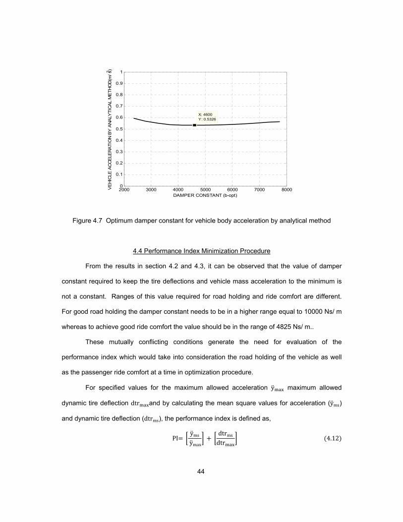
By following the same procedure as explained in section 4.2.2, the optimum value of

damper constant for minimum RMS vehicle acceleration is computed by analytical method (by

solving the integration for output PSD of vehicle acceleration). Following figure shows result of

the analytical method

2000 3000 4000 5000 6000 7000 8000 9000 10000 11000 12000 130000

0.1

0.2

0.3

0.4

0.5

0.6

0.7

0.8

0.9

1

X: 4825Y: 0.5888

DAMPER CONSTANT (Ns / m)

VE

HIC

LE A

CC

ELE

RA

TIO

N B

Y S

IMU

LATIO

N(m

/s2 )

44

Figure 4.7 Optimum damper constant for vehicle body acceleration by analytical method

4.4 Performance Index Minimization Procedure

From the results in section 4.2 and 4.3, it can be observed that the value of damper

constant required to keep the tire deflections and vehicle mass acceleration to the minimum is

not a constant. Ranges of this value required for road holding and ride comfort are different.

For good road holding the damper constant needs to be in a higher range equal to 10000 Ns/ m

whereas to achieve good ride comfort the value should be in the range of 4825 Ns/ m..

These mutually conflicting conditions generate the need for evaluation of the

performance index which would take into consideration the road holding of the vehicle as well

as the passenger ride comfort at a time in optimization procedure.

For specified values for the maximum allowed acceleration y maximum allowed

dynamic tire deflection dtr and by calculating the mean square values for acceleration (yms)

and dynamic tire deflection (dtrms), the performance index is defined as,

PI yms

ymax

dtrms

dtr 4.12

2000 3000 4000 5000 6000 7000 80000

0.1

0.2

0.3

0.4

0.5

0.6

0.7

0.8

0.9

1

X: 4600Y: 0.5326

DAMPER CONSTANT (b-opt)

VE

HIC

LE A

CC

ELE

RA

TIO

N B

Y A

NA

LYTIC

AL

ME

TH

OD

(m/ s2 )

45

Since the mean square values are divided by the respective maximum values, the performance

index is a dimensionless quantity. However, the values in the denominator need not be the

maximum values. These values can be used to normalize the dynamic tire deflection and

sprung mass acceleration and hence can be selected conveniently.

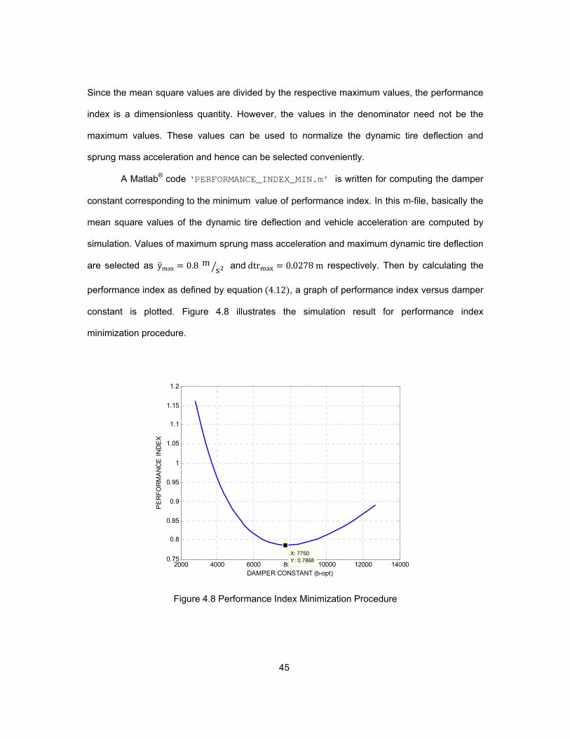
A Matlab® code ‘PERFORMANCE_INDEX_MIN.m’ is written for computing the damper

constant corresponding to the minimum value of performance index. In this m-file, basically the

mean square values of the dynamic tire deflection and vehicle acceleration are computed by

simulation. Values of maximum sprung mass acceleration and maximum dynamic tire deflection

are selected as ymax 0.8 m s and dtr 0.0278 m respectively. Then by calculating the

performance index as defined by equation 4.12 , a graph of performance index versus damper

constant is plotted. Figure 4.8 illustrates the simulation result for performance index

minimization procedure.

Figure 4.8 Performance Index Minimization Procedure

2000 4000 6000 8000 10000 12000 140000.75

0.8

0.85

0.9

0.95

1

1.05

1.1

1.15

1.2

X: 7750Y: 0.7868

DAMPER CONSTANT (b-opt)

PE

RF

OR

MA

NC

E I

ND

EX

46

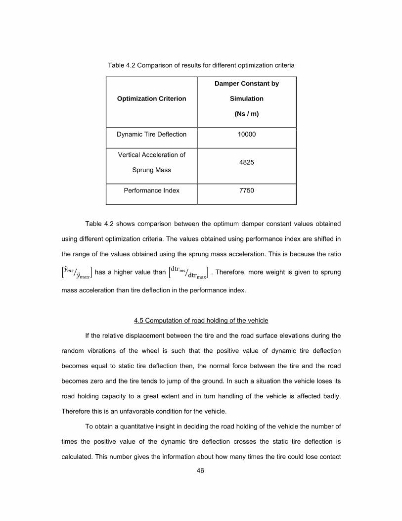
Table 4.2 Comparison of results for different optimization criteria

Optimization Criterion

Damper Constant by

Simulation

(Ns / m)

Dynamic Tire Deflection 10000

Vertical Acceleration of

Sprung Mass 4825

Performance Index 7750

Table 4.2 shows comparison between the optimum damper constant values obtained

using different optimization criteria. The values obtained using performance index are shifted in

the range of the values obtained using the sprung mass acceleration. This is because the ratio

has a higher value than dtrmsdtr . Therefore, more weight is given to sprung

mass acceleration than tire deflection in the performance index.

4.5 Computation of road holding of the vehicle

If the relative displacement between the tire and the road surface elevations during the

random vibrations of the wheel is such that the positive value of dynamic tire deflection

becomes equal to static tire deflection then, the normal force between the tire and the road

becomes zero and the tire tends to jump of the ground. In such a situation the vehicle loses its

road holding capacity to a great extent and in turn handling of the vehicle is affected badly.

Therefore this is an unfavorable condition for the vehicle.

To obtain a quantitative insight in deciding the road holding of the vehicle the number of

times the positive value of the dynamic tire deflection crosses the static tire deflection is

calculated. This number gives the information about how many times the tire could lose contact

47

with the ground per second. This can be calculated using following equation [10]. Let, p be

the number of positive crossings of the static tire deflection by the dynamic tire deflection.

p 1

2 π .

σ

σ e

4.12

Where,

σ - Standard deviation of the dynamic tire deflection

σ - First derivative of standard deviation of the dynamic tire deflection

d - Static tire deflection

Since all the equations of motion for the quarter car model are developed from the static

equilibrium position, the tires lose contact with the ground when the positive value of the

dynamic tire deflection becomes equal to the static tire deflection. The static deflection of the

tire is calculated as,

K . d M M . g

d 0.0278 m

The standard deviation of the dynamic tire deflection is computed by running the

simulation for of the quarter car model for a smooth highway for different values of the damper

constant. Substituting these values in equation 4.12 the number of positive crossings of the

tire deflection per second is calculated for each damper constant.

For example, consider the damper constant, b = 9550 Ns/ m

The output dynamic tire deflection by simulation is as shown in figure 4.9

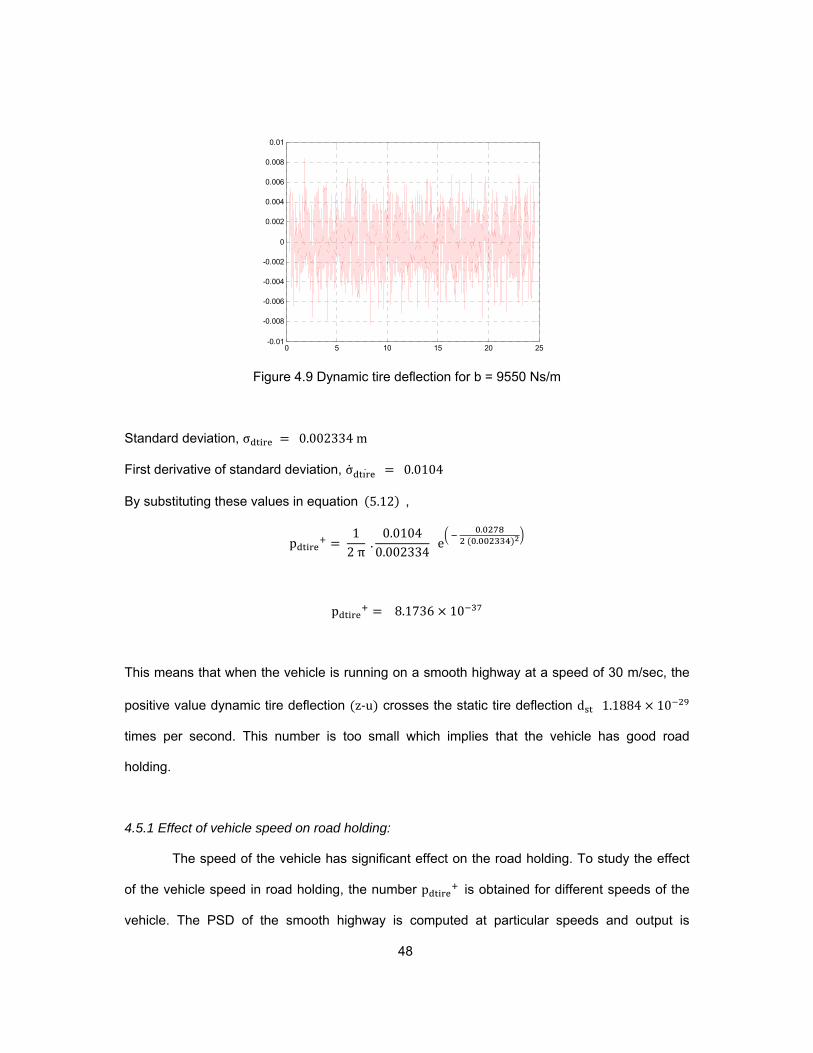
48

Figure 4.9 Dynamic tire deflection for b = 9550 Ns/m

Standard deviation, σ 0.002334 m

First derivative of standard deviation, σ 0.0104

By substituting these values in equation 5.12 ,

p 1

2 π .

0.01040.002334

e

. .

p 8.1736 10

This means that when the vehicle is running on a smooth highway at a speed of 30 m/sec, the

positive value dynamic tire deflection z‐u crosses the static tire deflection d 1.1884 10

times per second. This number is too small which implies that the vehicle has good road

holding.

4.5.1 Effect of vehicle speed on road holding:

The speed of the vehicle has significant effect on the road holding. To study the effect

of the vehicle speed in road holding, the number p is obtained for different speeds of the

vehicle. The PSD of the smooth highway is computed at particular speeds and output is

0 5 10 15 20 25-0.01

-0.008

-0.006

-0.004

-0.002

0

0.002

0.004

0.006

0.008

0.01

49

generated by simulation. The standard deviations for each output are then used for computing

the value of p by equation 4.12 .

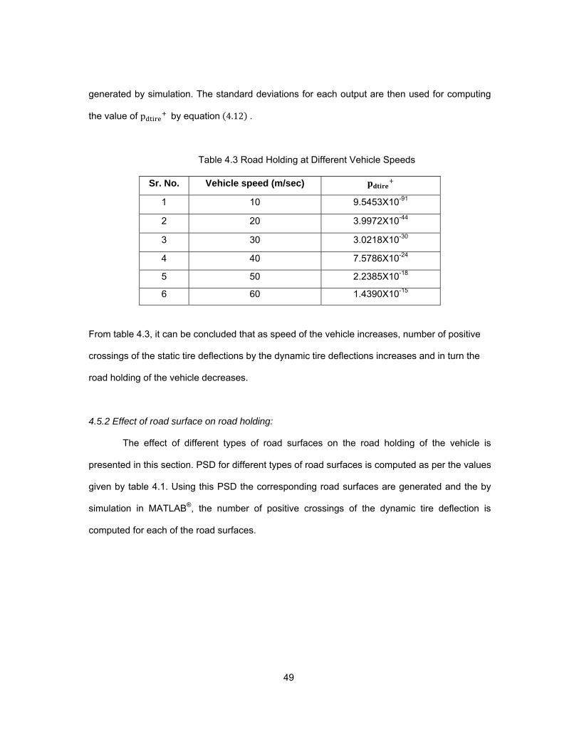
Table 4.3 Road Holding at Different Vehicle Speeds

From table 4.3, it can be concluded that as speed of the vehicle increases, number of positive

crossings of the static tire deflections by the dynamic tire deflections increases and in turn the

road holding of the vehicle decreases.

4.5.2 Effect of road surface on road holding:

The effect of different types of road surfaces on the road holding of the vehicle is

presented in this section. PSD for different types of road surfaces is computed as per the values

given by table 4.1. Using this PSD the corresponding road surfaces are generated and the by

simulation in MATLAB®, the number of positive crossings of the dynamic tire deflection is

computed for each of the road surfaces.

Sr. No. Vehicle speed (m/sec)

1 10 9.5453X10-91

2 20 3.9972X10-44

3 30 3.0218X10-30

4 40 7.5786X10-24

5 50 2.2385X10-18

6 60 1.4390X10-15

50

Smooth Runway RMS ( dtr ) = 0.1919 mm

Smooth Highway RMS ( dtr ) = 2.335 mm

Figure 4.10 Dynamic tire deflection for smooth runway and smooth highway

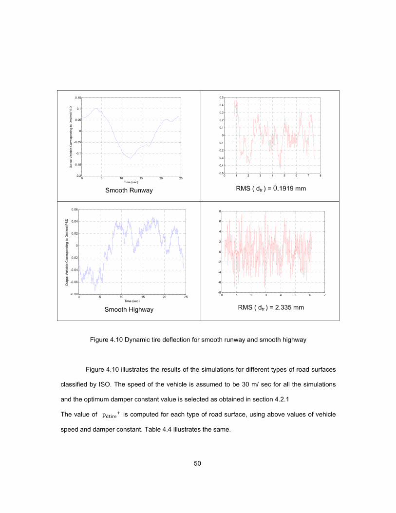
Figure 4.10 illustrates the results of the simulations for different types of road surfaces

classified by ISO. The speed of the vehicle is assumed to be 30 m/ sec for all the simulations

and the optimum damper constant value is selected as obtained in section 4.2.1

The value of p is computed for each type of road surface, using above values of vehicle

speed and damper constant. Table 4.4 illustrates the same.

0 5 10 15 20 25-0.08

-0.06

-0.04

-0.02

0

0.02

0.04

0.06

Time (sec)

Out

put

Var

iabl

e C

orre

spon

ding

to

Des

ired

PS

D

0 1 2 3 4 5 6 7-8

-6

-4

-2

0

2

4

6

8

0 5 10 15 20 25-0.2

-0.15

-0.1

-0.05

0

0.05

0.1

0.15

Time (sec)

Out

put

Var

iabl

e C

orre

spon

ding

to

Des

ired

PS

D

0 1 2 3 4 5 6 7 8-0.5

-0.4

-0.3

-0.2

-0.1

0

0.1

0.2

0.3

0.4

0.5

51

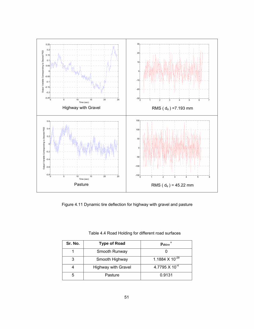
Highway with Gravel RMS ( dtr ) =7.193 mm

Pasture RMS ( dtr ) = 45.22 mm

Figure 4.11 Dynamic tire deflection for highway with gravel and pasture

Table 4.4 Road Holding for different road surfaces

0 5 10 15 20 25-0.25

-0.2

-0.15

-0.1

-0.05

0

0.05

0.1

0.15

0.2

0.25

Time (sec)

Out

put

Var

iabl

e C

orre

spon

ding

to

Des

ired

PS

D

0 1 2 3 4 5 6 7-30

-20

-10

0

10

20

30

0 5 10 15 20 25-0.8

-0.6

-0.4

-0.2

0

0.2

0.4

0.6

Time (sec)

Out

put

Var

iabl

e C

orre

spon

ding

to

Des

ired

PS

D

0 1 2 3 4 5 6-150

-100

-50

0

50

100

150

Sr. No. Type of Road

1 Smooth Runway 0

3 Smooth Highway 1.1884 X 10-29

4 Highway with Gravel 4.7795 X 10-4

5 Pasture 0.9131

52

From the table 4.4, it can be observed that as the roughness and irregularities of the

road surface increases, the number of positive crossings of the static tire deflection by the

positive value of the dynamic tire deflection increases. That is the tire tends to leave contact

with the ground more times per second. As a result, the road holding of the vehicle decreases.

53

CHAPTER 5

RESULTS AND CONCLUSION

1) This thesis illustrates a computer simulation based method for optimizing the suspension

system parameters for stationary stochastic inputs from uneven road surfaces. A computer

program using Matlab® has been created for generating random road surfaces with a given

power spectral density. Different performance characteristics of the suspension system

such as vertical acceleration of vehicle body, dynamic tire deflection can be evaluated by

numerical methods by exciting the system for generated random inputs.

2) The output results for the dynamic tire deflection are computed by analytical method by

integrating the PSD of the output between the limits of frequency range. The results

obtained by analytical method closely match with the results of numerical method. So, it can

be concluded that the numerical method of generating random time series can be

effectively used for simulation of the suspension system considering a quarter car model.

3) For good road holding of the vehicle, an optimum value of the damper constant is

computed. Results are obtained for number of simulations and it is observed that the

damper constant for good road holding is 10000 Ns/ m for the quarter car model under

consideration running on a smooth highway. Therefore good road holding and handling

requires a higher value of damping.

4) For passenger ride comfort, the optimum value of the damper constant obtained by

simulation results is 4825 Ns/ m over the entire frequency range. Therefore to achieve

better passenger ride comfort, lower value of shock absorber damping is required.

5) Optimization procedure by taking into consideration effect of vehicle mass acceleration and

dynamic tire deflection at the same time is possible by defining the performance index PI

54

as per equation 5.12 . Performance Index is a dimensionless quantity and the optimum

value of the damper constant can be found by minimizing the performance index.

6) A quantitative measure for deciding the roadholding of the vehicle has been proposed. A

number (p ) defined by equation 4.12 gives the frequency of crossing the static tire

deflection by the dynamic tire deflections per second and is used to evaluate the road

holding of the vehicle

7) Value of p is computed for different speeds of the vehicle for a smooth highway. It is

observed that the road holding of the tires decrease with increase in the speed.

8) Value of p is computed for different types of road surfaces such as smooth runway,

smooth highway, highway with gravel and pasture. It is shown numerically that as the road

roughness increases, the road holding of the tires decrease.

55

APPENDIX A

MATLAB® FILES FOR USED FOR GENERATING STOCHASTIC INPUTS AND OUTPUT RESPONSES

IN TIME DOMAIN

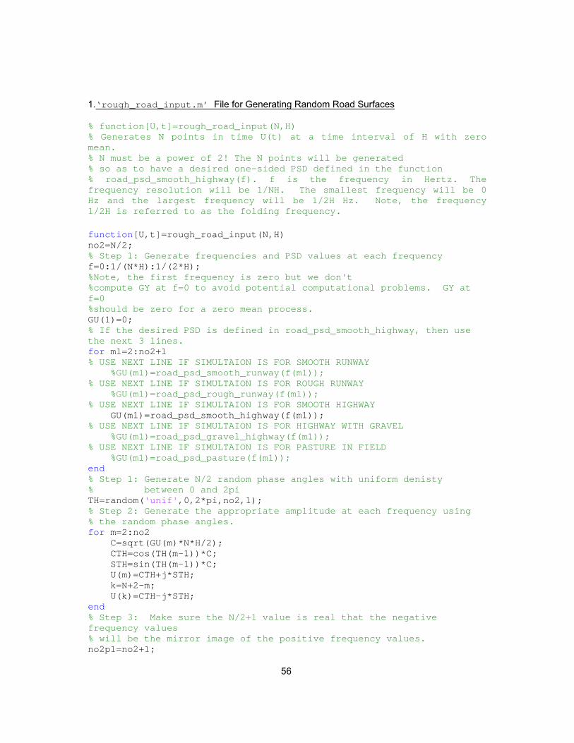
56

1.‘rough_road_input.m’ File for Generating Random Road Surfaces

% function[U,t]=rough_road_input(N,H) % Generates N points in time U(t) at a time interval of H with zero mean. % N must be a power of 2! The N points will be generated % so as to have a desired one-sided PSD defined in the function % road_psd_smooth_highway(f). f is the frequency in Hertz. The frequency resolution will be 1/NH. The smallest frequency will be 0 Hz and the largest frequency will be 1/2H Hz. Note, the frequency 1/2H is referred to as the folding frequency. function[U,t]=rough_road_input(N,H) no2=N/2; % Step 1: Generate frequencies and PSD values at each frequency f=0:1/(N*H):1/(2*H); %Note, the first frequency is zero but we don't %compute GY at f=0 to avoid potential computational problems. GY at f=0 %should be zero for a zero mean process. GU(1)=0; % If the desired PSD is defined in road_psd_smooth_highway, then use the next 3 lines. for m1=2:no2+1 % USE NEXT LINE IF SIMULTAION IS FOR SMOOTH RUNWAY %GU(m1)=road_psd_smooth_runway(f(m1)); % USE NEXT LINE IF SIMULTAION IS FOR ROUGH RUNWAY %GU(m1)=road_psd_rough_runway(f(m1)); % USE NEXT LINE IF SIMULTAION IS FOR SMOOTH HIGHWAY GU(m1)=road_psd_smooth_highway(f(m1)); % USE NEXT LINE IF SIMULTAION IS FOR HIGHWAY WITH GRAVEL %GU(m1)=road_psd_gravel_highway(f(m1)); % USE NEXT LINE IF SIMULTAION IS FOR PASTURE IN FIELD %GU(m1)=road_psd_pasture(f(m1)); end % Step 1: Generate N/2 random phase angles with uniform denisty % between 0 and 2pi TH=random('unif',0,2*pi,no2,1); % Step 2: Generate the appropriate amplitude at each frequency using % the random phase angles. for m=2:no2 C=sqrt(GU(m)*N*H/2); CTH=cos(TH(m-1))*C; STH=sin(TH(m-1))*C; U(m)=CTH+j*STH; k=N+2-m; U(k)=CTH-j*STH; end % Step 3: Make sure the N/2+1 value is real that the negative frequency values % will be the mirror image of the positive frequency values. no2p1=no2+1;

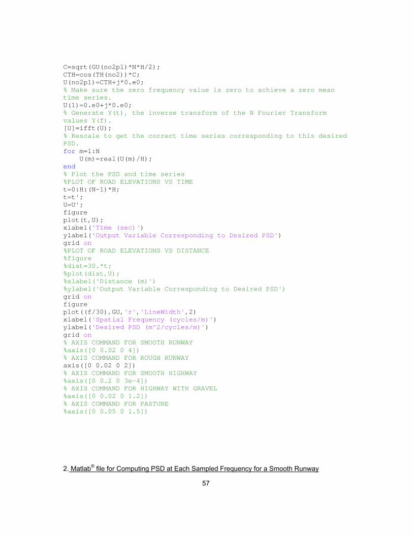
57

C=sqrt(GU(no2p1)*N*H/2); CTH=cos(TH(no2))*C; U(no2p1)=CTH+j*0.e0; % Make sure the zero frequency value is zero to achieve a zero mean time series. U(1)=0.e0+j*0.e0; % Generate Y(t), the inverse transform of the N Fourier Transform values Y(f). [U]=ifft(U); % Rescale to get the correct time series corresponding to this desired PSD. for m=1:N U(m)=real(U(m)/H); end % Plot the PSD and time series %PLOT OF ROAD ELEVATIONS VS TIME t=0:H:(N-1)*H; t=t'; U=U'; figure plot(t,U); xlabel('Time (sec)') ylabel('Output Variable Corresponding to Desired PSD') grid on %PLOT OF ROAD ELEVATIONS VS DISTANCE %figure %dist=30.*t; %plot(dist,U); %xlabel('Distance (m)') %ylabel('Output Variable Corresponding to Desired PSD') grid on figure plot((f/30),GU,'r','LineWidth',2) xlabel('Spatial Frequency (cycles/m)') ylabel('Desired PSD (m^2/cycles/m)') grid on % AXIS COMMAND FOR SMOOTH RUNWAY %axis([0 0.02 0 4]) % AXIS COMMAND FOR ROUGH RUNWAY axis([0 0.02 0 2]) % AXIS COMMAND FOR SMOOTH HIGHWAY %axis([0 0.2 0 3e-4]) % AXIS COMMAND FOR HIGHWAY WITH GRAVEL %axis([0 0.02 0 1.2]) % AXIS COMMAND FOR PASTURE %axis([0 0.05 0 1.5])

2. Matlab® file for Computing PSD at Each Sampled Frequency for a Smooth Runway

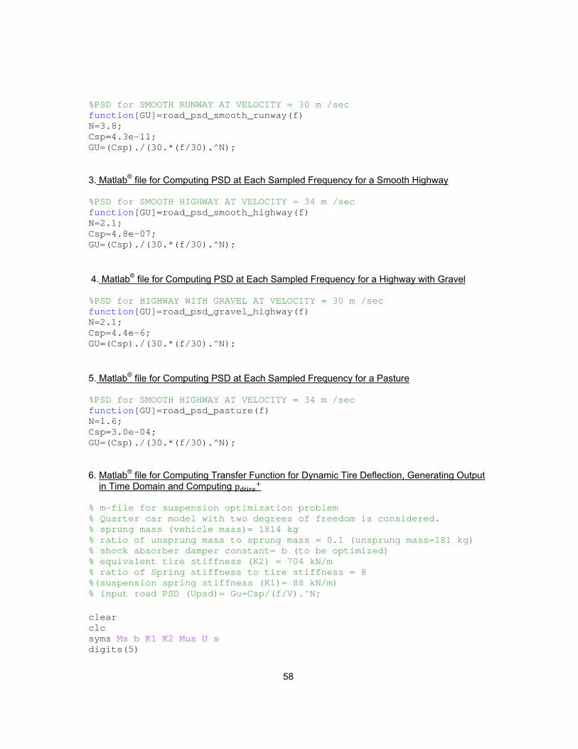
58

%PSD for SMOOTH RUNWAY AT VELOCITY = 30 m /sec function[GU]=road_psd_smooth_runway(f) N=3.8; Csp=4.3e-11; GU=(Csp)./(30.*(f/30).^N);

3. Matlab® file for Computing PSD at Each Sampled Frequency for a Smooth Highway

%PSD for SMOOTH HIGHWAY AT VELOCITY = 34 m /sec function[GU]=road_psd_smooth_highway(f) N=2.1; Csp=4.8e-07; GU=(Csp)./(30.*(f/30).^N);

4. Matlab® file for Computing PSD at Each Sampled Frequency for a Highway with Gravel

%PSD for HIGHWAY WITH GRAVEL AT VELOCITY = 30 m /sec function[GU]=road_psd_gravel_highway(f) N=2.1; Csp=4.4e-6; GU=(Csp)./(30.*(f/30).^N);

5. Matlab® file for Computing PSD at Each Sampled Frequency for a Pasture

%PSD for SMOOTH HIGHWAY AT VELOCITY = 34 m /sec function[GU]=road_psd_pasture(f) N=1.6; Csp=3.0e-04; GU=(Csp)./(30.*(f/30).^N); 6. Matlab® file for Computing Transfer Function for Dynamic Tire Deflection, Generating Output in Time Domain and Computing p % m-file for suspension optimization problem % Quarter car model with two degrees of freedom is considered. % sprung mass (vehicle mass)= 1814 kg % ratio of unsprung mass to sprung mass = 0.1 (unsprung mass=181 kg) % shock absorber damper constant= b (to be optimized) % equivalent tire stiffness (K2) = 704 kN/m % ratio of Spring stiffness to tire stiffness = 8 %(suspension spring stiffness (K1)= 88 kN/m) % input road PSD (Upsd)= Gu=Csp/(f/V).^N; clear clc syms Ms b K1 K2 Mus U s digits(5)

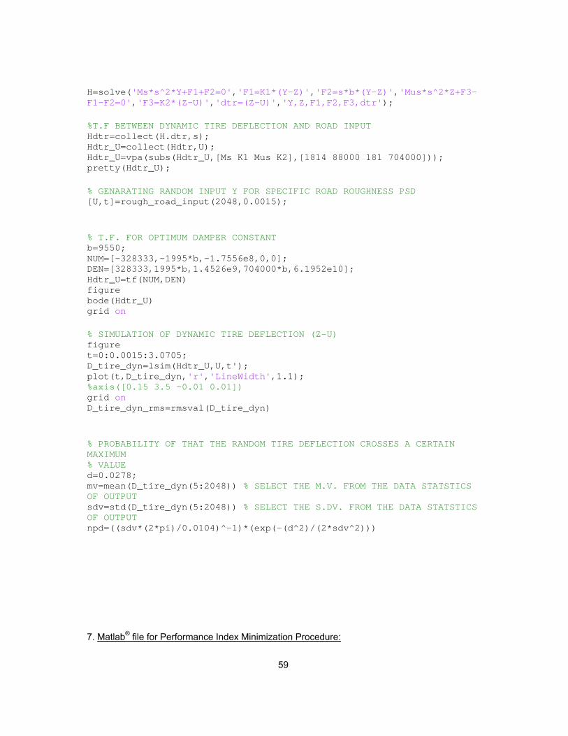
59

H=solve('Ms*s^2*Y+F1+F2=0','F1=K1*(Y-Z)','F2=s*b*(Y-Z)','Mus*s^2*Z+F3-F1-F2=0','F3=K2*(Z-U)','dtr=(Z-U)','Y,Z,F1,F2,F3,dtr'); %T.F BETWEEN DYNAMIC TIRE DEFLECTION AND ROAD INPUT Hdtr=collect(H.dtr,s); Hdtr_U=collect(Hdtr,U); Hdtr_U=vpa(subs(Hdtr_U,[Ms K1 Mus K2],[1814 88000 181 704000])); pretty(Hdtr_U); % GENARATING RANDOM INPUT Y FOR SPECIFIC ROAD ROUGHNESS PSD [U,t]=rough_road_input(2048,0.0015); % T.F. FOR OPTIMUM DAMPER CONSTANT b=9550; NUM=[-328333,-1995*b,-1.7556e8,0,0]; DEN=[328333,1995*b,1.4526e9,704000*b,6.1952e10]; Hdtr_U=tf(NUM,DEN) figure bode(Hdtr_U) grid on % SIMULATION OF DYNAMIC TIRE DEFLECTION (Z-U) figure t=0:0.0015:3.0705; D_tire_dyn=lsim(Hdtr_U,U,t'); plot(t,D_tire_dyn,'r','LineWidth',1.1); %axis([0.15 3.5 -0.01 0.01]) grid on D_tire_dyn_rms=rmsval(D_tire_dyn) % PROBABILITY OF THAT THE RANDOM TIRE DEFLECTION CROSSES A CERTAIN MAXIMUM % VALUE d=0.0278; mv=mean(D_tire_dyn(5:2048)) % SELECT THE M.V. FROM THE DATA STATSTICS OF OUTPUT sdv=std(D_tire_dyn(5:2048)) % SELECT THE S.DV. FROM THE DATA STATSTICS OF OUTPUT npd=((sdv*(2*pi)/0.0104)^-1)*(exp(-(d^2)/(2*sdv^2)))

7. Matlab® file for Performance Index Minimization Procedure:

60

%% OPTIMIZING THE DAMPER CONSTNT CONSIDERING BOTH OF THE VEHICLE %% ACCELERATION AS WELL AS DYNAMIC TIRE DEFLECTION BY DEFINING A COST %% FUNCTION clear clc % GENARATING RANDOM INPUT Y FOR SPECIFIC ROAD ROUGHNESS PSD [U,t]=rough_road_input(16384,0.0015); n=1; % MAXIMUM ALLOWED TIRE DEFLECTION AND VEH ACCN dtr_max= 0.002; ydd_max=0.80; %RMS VEHICLE ACCELERATION for b1=2800:225:12700 NUM1=[704000*b1,6.1952e10,0,0]; DEN1=[328333,1995*b1,1.4526e9,704000*b1,6.1952e10]; HYddm_U=tf(NUM1,DEN1); % SIMULATION OF VEHICLE ACCELERATION %figure t=0:0.0015:24.5745; VEH_ACCN=lsim(HYddm_U,U,t'); VEH_ACCN_rms_numerical(:,n)=rmsval(VEH_ACCN); if n<45 n=n+1; end end % PLOT OF RMS VALUE OF THE VEHICLE ACCELERATION VS DAMPER CONSTANT %b=2800:225:12700; %figure %plot(b,VEH_ACCN_rms_numerical,'k','LineWidth',2); %xlabel('DAMPER CONSTANT (b-opt)') %ylabel('VEHICLE FORCE BY SIMULATION(m)') %grid on % RMS DYNAMIC TIRE DEFLECTI0N m=1; for b=2800:225:12700 NUM=[-328333,-1995*b,-1.7556e8,0,0]; DEN=[328333,1995*b,1.4526e9,704000*b,6.1952e10]; HRH_U=tf(NUM,DEN); % SIMULATION OF DYNAMIC TIRE DEFLECTION %figure

61

t=0:0.0015:24.5745; TIRE_DFLN=lsim(HRH_U,U,t'); TIRE_DFLN_rms_numerical(:,m)=rmsval(TIRE_DFLN); if m<45 m=m+1; end end % PLOT OF RMS VALUE OF THE DYNAMIC TIRE DEFLECTION VS DAMPER CONSTANT %b=2800:225:12700; %figure %plot(b,TIRE_DFLN_rms_numerical,'k','LineWidth',2); %xlabel('DAMPER CONSTANT (b-opt)') %ylabel('DYNAMIC TIRE DEFLECTION BY SIMULATION(m)') %grid on % COST FUNCTION mstd=TIRE_DFLN_rms_numerical.^2; msydd=VEH_ACCN_rms_numerical.^2; CF=(mstd./(dtr_max^2))+(msydd./(ydd_max)^2); %PI=(ydd_max^2/dtr_max^2).*(mstd)+msydd b=2800:225:12700; figure plot(b,PI,'b','LineWidth',1.5); xlabel('DAMPER CONSTANT (b-opt)') ylabel('COST FUNCTION') grid on 8. Matlab® file for Calculating First Derivative of Standard Deviation of Dynamic tire Deflection (σ ): syms s TF=(-328333*s^5-1.905e7*s^4-1.756e8*s^3)/(328333*s^4+1.905e7*s^4+1.453e9*s^2+6.723e9*s+6.195e10); syms f %SMOOTH RUNWAY GUU=5.8804e-7/f^4; msval=msv(TF,GUU,0.5,300); sigma_dot=sqrt(real(msval)) %SMOOTH HIGHWAY GUU=2.0234e-5/f^2; msval=msv(TF,GUU,0.5,300); sigma_dot=sqrt(real(msval)) %GRAVEL HIGHWAY GUU=1.8547e-4/f^2; msval=msv(TF,GUU,0.5,300);

62

sigma_dot=sqrt(real(msval)) %SMOOTH HIGHWAY GUU=2.3088e-3/f^1.5; msval=msv(TF,GUU,0.5,300); sigma_dot=sqrt(real(msval))

63

REFERENCES

1. Julius S. Bendat and Allen G. Piersol, ‘Random Data: Analysis and Measurement

Procedures’, Wiley-Interscience Publications

2. J. Y. Wong, ‘Theory of Ground Vehicles (fourth edition)’, Wiley Publications

3. Dr. D. A. Hullender, ‘Generation of a Random Time Series with a Specified Spectral Density

Function’, University of Texas at Arlington, submitted through ASME for JACC, 1979

4. ‘Estimation of Disturbance Inputs to a Tire Coupled Quarter Car Suspension Test Rig’,

Thesis by Jonathan D. Zeigenmeyer, Virginia Polytechnic Institute & State University, 2007

5. ‘Vibration Transmission from Road Surface Features-Vehicle Measurement and Detection’,

Technical report for Nissan Technical Center North America Inc. by Timothy J. Gordon and

Zevi Bareket, The University of Michigan Transportation Research Institute, 2007

6. ‘Optimal Design for Passenger Car Suspension for Ride and Road Holding’ by Anil Shirhatt,

P.S.S. Prasad, Pravin Panzade, M.M. Kulkarni

7. ‘Model Complexity Requirements In Design Of Half Car Active Suspension Controllers’,

Keith J. Wakeham and D. Geoff Rideout, Memorial University, Department of Engineering

and Applied Sciences, Canada

8. ‘Generation of Virtual Road Surfaces and Simulation of Nonlinear Vibration of Vehicles’,

IEEE Paper by Song Jian, Jin Ruichen, Department of Automotive Engineering, Tsinghua

University, China

9. ‘Non-stationary Random Vibration Analysis of Vehicle with Fractional Damping’, Yunqing

Zhang, Wei Chen, Liping Chen, Wenbin Shangguan,

10. ‘Modeling and Simulation of Engineering Systems’, Course Notebook for Dynamic Systems

Modeling, Prof. D. A. Hullender

64

BIOGRAPHICAL INFORMATION

Kailas has completed his bachelor in Mechanical Engineering from VIT, University of

Pune, India. He has worked as an engineer in Larsen & Toubro Limited, India in design and

engineering of process gas boiler systems. His research interests include applied mechanics,

multi-body dynamics and noise and vibration analysis.