Vertical distribution of ozone at four sites in the United ... · Vertical distribution of ozone at four sites in the United ... The vertical distribution of ozone throughout the

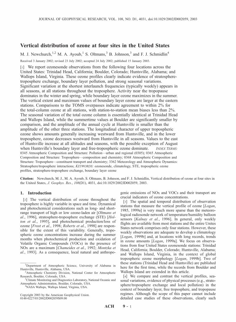
Vertical distribution of ozone at four sites in the United States

M. J. Newchurch,1,2 M. A. Ayoub,1 S. Oltmans,3 B. Johnson,3 and F. J. Schmidlin4

Received 3 January 2002; revised 23 July 2002; accepted 24 July 2002; published 15 January 2003.

[1] We report ozonesonde observations from the following four locations across theUnited States: Trinidad Head, California; Boulder, Colorado; Huntsville, Alabama; andWallops Island, Virginia. These ozone profiles clearly indicate evidence of stratosphere-troposphere exchange, boundary layer pollution, and strong seasonal variations.Significant variation at the shortest interlaunch frequencies (typically weekly) appears inall seasons, at all stations throughout the troposphere. Activity near the tropopausedominates in the winter and spring, while boundary layer ozone maximizes in the summer.The vertical extent and maximum values of boundary layer ozone are larger at the easternstations. Comparisons to the TOMS overpasses indicate agreement to within 2% forthe total-column ozone at all stations, with station-to-station mean biases less than 2%.The seasonal variation of the total ozone column is essentially identical at Trinidad Headand Wallops Island, while the summertime values at Boulder are significantly smaller bycomparison, and the amplitude of the annual cycle at Huntsville is smaller than theamplitude of the other three stations. The longitudinal character of upper troposphericozone shows amounts generally increasing westward from Huntsville, and in the lowertroposphere, ozone decreases westward from Huntsville in all seasons. Values to the eastof Huntsville increase at all altitudes and seasons, with the possible exception of Augustwhen Huntsville’s boundary layer and free-tropospheric ozone dominate. INDEX TERMS:

0345 Atmospheric Composition and Structure: Pollution—urban and regional (0305); 0365 Atmospheric

Composition and Structure: Troposphere—composition and chemistry; 0368 Atmospheric Composition and

Structure: Troposphere—constituent transport and chemistry; 3362 Meteorology and Atmospheric Dynamics:

Stratosphere/troposphere interactions; KEYWORDS: ozonesonde, climatology, STE, tropospheric ozone

profiles, stratosphere-troposphere exchange, boundary layer ozone

Citation: Newchurch, M. J., M. A. Ayoub, S. Oltmans, B. Johnson, and F. J. Schmidlin, Vertical distribution of ozone at four sites in

the United States, J. Geophys. Res., 108(D1), 4031, doi:10.1029/2002JD002059, 2003.

1. Introduction

[2] The vertical distribution of ozone throughout thetroposphere is highly variable in space and time. Dynamicaland photochemical considerations such as long- and short-range transport of high or low ozone-laden air [Oltmans etal., 1996], stratosphere-troposphere exchange (STE) [Hol-ton et al., 1995], and photochemical production/loss ofozone [Frost et al., 1998; Roberts et al., 1998] are respon-sible for the extent of this variability. Generally, tropo-spheric ozone concentrations increase during the summermonths when photochemical production and oxidation ofVolatile Organic Compounds (VOCs) in the presence ofNOx are a maximum [Chameides et al., 1992; Montzka etal., 1993]. As a consequence, local natural and anthropo-

genic emissions of NOx and VOCs and their transport arecrucial indicators of ozone concentrations.[3] The spatial and temporal distribution of observation

stations that measure the vertical profile of ozone [Logan,1985, 1999a] is very much more sparse than the meteoro-logical radiosonde network of temperature/humidity balloonsensors [Kalnay et al., 1996]. In general, only weeklyflights are available from most stations and the entire UnitesStates network comprises only four stations. However, theseweekly observations are adequate to develop a climatology[Logan, 1999b] and, at locations with long records, trendsin ozone amounts [Logan, 1999a]. We focus on observa-tions from four United States ozonesonde stations: TrinidadHead, California; Boulder, Colorado; Huntsville, Alabama;and Wallops Island, Virginia, in the context of globaltropospheric ozone morphology [Logan, 1999b]. Two ofthese stations (Trinidad Head and Huntsville) are publishedhere for the first time, while the records from Boulder andWallops Island are extended in this article.[4] We compare and contrast the vertical profiles, sea-

sonal variations, evidence of physical processes (e.g., strato-sphere/troposphere exchange and local pollution) in thecontext of boundary layer, free troposphere, and tropopauseregimes. Although the scope of this paper cannot includedetailed case studies of these observations, clearly such

JOURNAL OF GEOPHYSICAL RESEARCH, VOL. 108, NO. D1, 4031, doi:10.1029/2002JD002059, 2003

1Department of Atmospheric Science, University of Alabama inHuntsville, Huntsville, Alabama, USA.

2Atmospheric Chemistry Division, National Center for AtmosphericResearch, Boulder, Colorado, USA.

3Climate Monitoring and Diagnostics Laboratory, National Oceanic andAtmospheric Administration, Boulder, Colorado, USA.

4NASA Wallops, Wallops Island, Virginia, USA.

Copyright 2003 by the American Geophysical Union.0148-0227/03/2002JD002059$09.00

ACH 9 - 1

studies are warranted from this initial description of theozone vertical morphology.

2. Measurements

[5] Vertical profiles of ozone partial pressure, ambientpressure, temperature, and dew point are measured byballoon-borne ozonesondes employing an ElectrochemicalConcentration Cell (ECC) sensor [Komhyr, 1969] and anRS-80 Vaisala or Sippican Inc. MK-2 radiosonde. Theballoons ascend, on average, to altitudes of 30–35 km (6hPa), providing accurate in situ measurements of 95% of theentire atmospheric ozone column. Although high temporal-and spatial-resolution launches are currently unavailable,long-term data at select locations around the world providean essential source for accurate characterization of climato-logical patterns at all atmospheric levels [Beekmann et al.,1994; Fortuin and Kelder, 1998; Logan, 1999b; McPeterset al., 1997; Thompson et al., 2001] and provide validationtools for a number of ozone-measuring satellites [Attmanns-pacher et al., 1989; Brinksma et al., 2000; Cunnold et al.,1989; Hoogen et al., 1999; Kim et al., 2001; Lucke et al.,1999; Margitan et al., 1995; Newchurch et al., 2001a,2001b; Sasano et al., 1999].[6] The electrochemical concentration cell (ECC) sensor

used at all these stations has been extensively tested andcompared to other instruments and is in wide use [Johnsonet al., 2002; Komhyr et al., 1995; Reid et al., 1996; Tarasicket al., 1996]. The three NOAA/CMDL stations, TrinidadHead, Boulder, and Huntsville, use the EN-SCI model 2Zozonesondes, with 2% unbuffered potassium iodide (KI)cathode solution. Since 1996, the NASA Wallops FlightFacility has used both EN-SCI model Z ECCs and SciencePump Corporation models 5a and 6a ECCs. Both types ofECCs are compatible with Sippican MK-2 radiosondes withboth Loran-C wind finding capability and GPS (LOS) [(-y-zpositions). Since late 1994, Wallops Flight Facility has beenusing 1% buffered KI solution.[7] ECC sonde accuracies are about 10% for tropospheric

mixing ratios, except in the case of very low mixing ratios(<10 ppb) when the accuracy may be degraded to 15%.Although the reaction with potassium iodide is not specific toozone, concentrations of interfering species such as NO2 andSO2 are usually in the sub-ppb ranges and, hence, do notconstitute a significant interferent [Oltmans et al., 1996].[8] Vertical profiles are obtained from weekly balloon

launches and occasional more frequent launches at all fourof the ozonesonde locations. The Wallops Island measure-ments began in 1970, and the Boulder soundings started in1979. Programs at both of these sites have had someinterruptions over this period but represent relatively longtime series. The station at Trinidad Head was initiated inAugust 1997, and the Huntsville ozonesonde station com-menced operation in April 1999. The station at WallopsIsland is operated by the Upper Air InstrumentationResearch Project, Observational Science Branch of theLaboratory for Hydrospheric Processes at the Wallops FlightFacility of NASA. The NOAA Climate Monitoring andDiagnostics Laboratory (CMDL) launch the soundings atBoulder. At Trinidad Head the soundings are a cooperativeeffort between CMDL and the Humboldt State UniversityMarine Sciences Laboratory. The Huntsville ozonesonde

station is a joint effort between the Earth System ScienceCenter of the University of Alabama at Huntsville andCMDL. Data are available from the World Ozone andUltraviolet Radiation Data Centre (WOUDC) for WallopsIsland (Station Number 107), Boulder (067), and Huntsville(418) at http://www.msc-smc.ec.gc.ca/woudc. In addition,plots and/or data are available for Wallops Island at http://uairp.wff.nasa.gov; for Huntsville at http://www.nsstc.uah.edu/atmchem; and for Boulder, Trinidad Head, and Hunts-ville at http://www.cmdl.noaa.gov/info/ftpdata.html.[9] Trinidad Head lies on the northwest coast of Califor-

nia and experiences predominantly air characteristic of thePacific basin. Boulder is a high-altitude midsize city that isdownwind of the Denver metropolitan area under south-easterly wind conditions. Huntsville lies in the southeasternunited states, a region with abundant deciduous trees.Nearby cities include Birmingham, AL (130 km due South,)Nashville, TN (180 km due North,) and Atlanta, GA (370km due southeast.) Wallops Island lies on the northeastcoast of the United States and often experiences pollutedcontinental air.

3. Results and Discussion

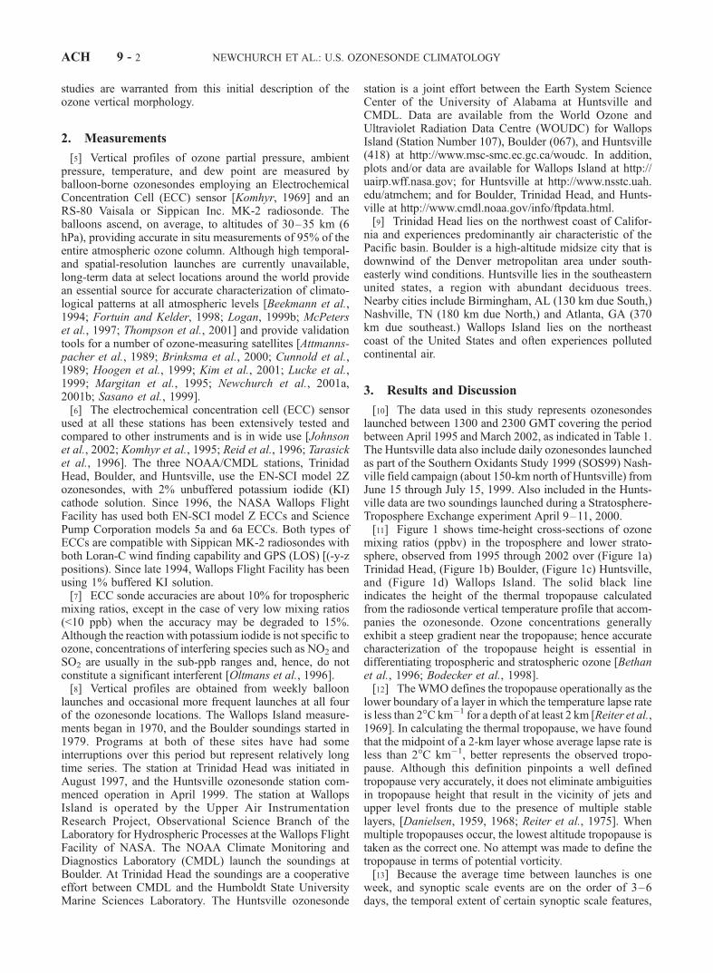
[10] The data used in this study represents ozonesondeslaunched between 1300 and 2300 GMT covering the periodbetween April 1995 and March 2002, as indicated in Table 1.The Huntsville data also include daily ozonesondes launchedas part of the Southern Oxidants Study 1999 (SOS99) Nash-ville field campaign (about 150-km north of Huntsville) fromJune 15 through July 15, 1999. Also included in the Hunts-ville data are two soundings launched during a Stratosphere-Troposphere Exchange experiment April 9–11, 2000.[11] Figure 1 shows time-height cross-sections of ozone

mixing ratios (ppbv) in the troposphere and lower strato-sphere, observed from 1995 through 2002 over (Figure 1a)Trinidad Head, (Figure 1b) Boulder, (Figure 1c) Huntsville,and (Figure 1d) Wallops Island. The solid black lineindicates the height of the thermal tropopause calculatedfrom the radiosonde vertical temperature profile that accom-panies the ozonesonde. Ozone concentrations generallyexhibit a steep gradient near the tropopause; hence accuratecharacterization of the tropopause height is essential indifferentiating tropospheric and stratospheric ozone [Bethanet al., 1996; Bodecker et al., 1998].[12] TheWMO defines the tropopause operationally as the

lower boundary of a layer in which the temperature lapse rateis less than 2�C km�1 for a depth of at least 2 km [Reiter et al.,1969]. In calculating the thermal tropopause, we have foundthat the midpoint of a 2-km layer whose average lapse rate isless than 2�C km�1, better represents the observed tropo-pause. Although this definition pinpoints a well definedtropopause very accurately, it does not eliminate ambiguitiesin tropopause height that result in the vicinity of jets andupper level fronts due to the presence of multiple stablelayers, [Danielsen, 1959, 1968; Reiter et al., 1975]. Whenmultiple tropopauses occur, the lowest altitude tropopause istaken as the correct one. No attempt was made to define thetropopause in terms of potential vorticity.[13] Because the average time between launches is one

week, and synoptic scale events are on the order of 3–6days, the temporal extent of certain synoptic scale features,

ACH 9 - 2 NEWCHURCH ET AL.: U.S. OZONESONDE CLIMATOLOGY

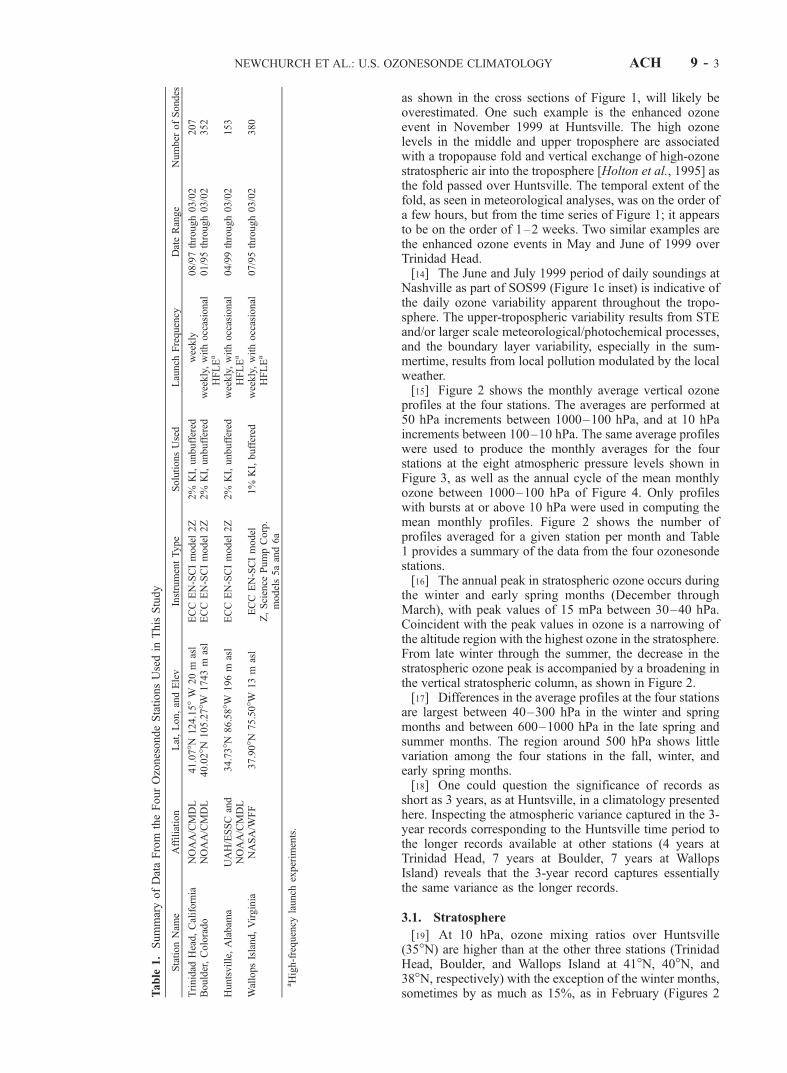
as shown in the cross sections of Figure 1, will likely beoverestimated. One such example is the enhanced ozoneevent in November 1999 at Huntsville. The high ozonelevels in the middle and upper troposphere are associatedwith a tropopause fold and vertical exchange of high-ozonestratospheric air into the troposphere [Holton et al., 1995] asthe fold passed over Huntsville. The temporal extent of thefold, as seen in meteorological analyses, was on the order ofa few hours, but from the time series of Figure 1; it appearsto be on the order of 1–2 weeks. Two similar examples arethe enhanced ozone events in May and June of 1999 overTrinidad Head.[14] The June and July 1999 period of daily soundings at

Nashville as part of SOS99 (Figure 1c inset) is indicative ofthe daily ozone variability apparent throughout the tropo-sphere. The upper-tropospheric variability results from STEand/or larger scale meteorological/photochemical processes,and the boundary layer variability, especially in the sum-mertime, results from local pollution modulated by the localweather.[15] Figure 2 shows the monthly average vertical ozone

profiles at the four stations. The averages are performed at50 hPa increments between 1000–100 hPa, and at 10 hPaincrements between 100–10 hPa. The same average profileswere used to produce the monthly averages for the fourstations at the eight atmospheric pressure levels shown inFigure 3, as well as the annual cycle of the mean monthlyozone between 1000–100 hPa of Figure 4. Only profileswith bursts at or above 10 hPa were used in computing themean monthly profiles. Figure 2 shows the number ofprofiles averaged for a given station per month and Table1 provides a summary of the data from the four ozonesondestations.[16] The annual peak in stratospheric ozone occurs during

the winter and early spring months (December throughMarch), with peak values of 15 mPa between 30–40 hPa.Coincident with the peak values in ozone is a narrowing ofthe altitude region with the highest ozone in the stratosphere.From late winter through the summer, the decrease in thestratospheric ozone peak is accompanied by a broadening inthe vertical stratospheric column, as shown in Figure 2.[17] Differences in the average profiles at the four stations

are largest between 40–300 hPa in the winter and springmonths and between 600–1000 hPa in the late spring andsummer months. The region around 500 hPa shows littlevariation among the four stations in the fall, winter, andearly spring months.[18] One could question the significance of records as

short as 3 years, as at Huntsville, in a climatology presentedhere. Inspecting the atmospheric variance captured in the 3-year records corresponding to the Huntsville time period tothe longer records available at other stations (4 years atTrinidad Head, 7 years at Boulder, 7 years at WallopsIsland) reveals that the 3-year record captures essentiallythe same variance as the longer records.

3.1. Stratosphere

[19] At 10 hPa, ozone mixing ratios over Huntsville(35�N) are higher than at the other three stations (TrinidadHead, Boulder, and Wallops Island at 41�N, 40�N, and38�N, respectively) with the exception of the winter months,sometimes by as much as 15%, as in February (Figures 2T

able

1.SummaryofDataFrom

theFourOzonesondeStationsUsedin

ThisStudy

StationNam

eAffiliation

Lat,Lon,andElev

InstrumentType

SolutionsUsed

Launch

Frequency

DateRange

Number

ofSondes

Trinidad

Head,California

NOAA/CMDL

41.07�N

124.15�W

20m

asl

ECCEN-SCImodel

2Z

2%

KI,unbuffered

weekly

08/97through03/02

207

Boulder,Colorado

NOAA/CMDL

40.02�N

105.27�W

1743m

asl

ECCEN-SCImodel

2Z

2%

KI,unbuffered

weekly,withoccasional

HFLEa

01/95through03/02

352

Huntsville,Alabam

aUAH/ESSCand

NOAA/CMDL

34.73�N

86.58�W

196m

asl

ECCEN-SCImodel

2Z

2%

KI,unbuffered


HFLEa

04/99through03/02

153

WallopsIsland,Virginia

NASA/W

FF

37.90�N

75.50�W

13m

asl

ECCEN-SCImodel

Z,Science

PumpCorp.

models5aand6a

1%

KI,buffered


HFLEa

07/95through03/02

380

aHigh-frequency

launch

experim

ents.

NEWCHURCH ET AL.: U.S. OZONESONDE CLIMATOLOGY ACH 9 - 3

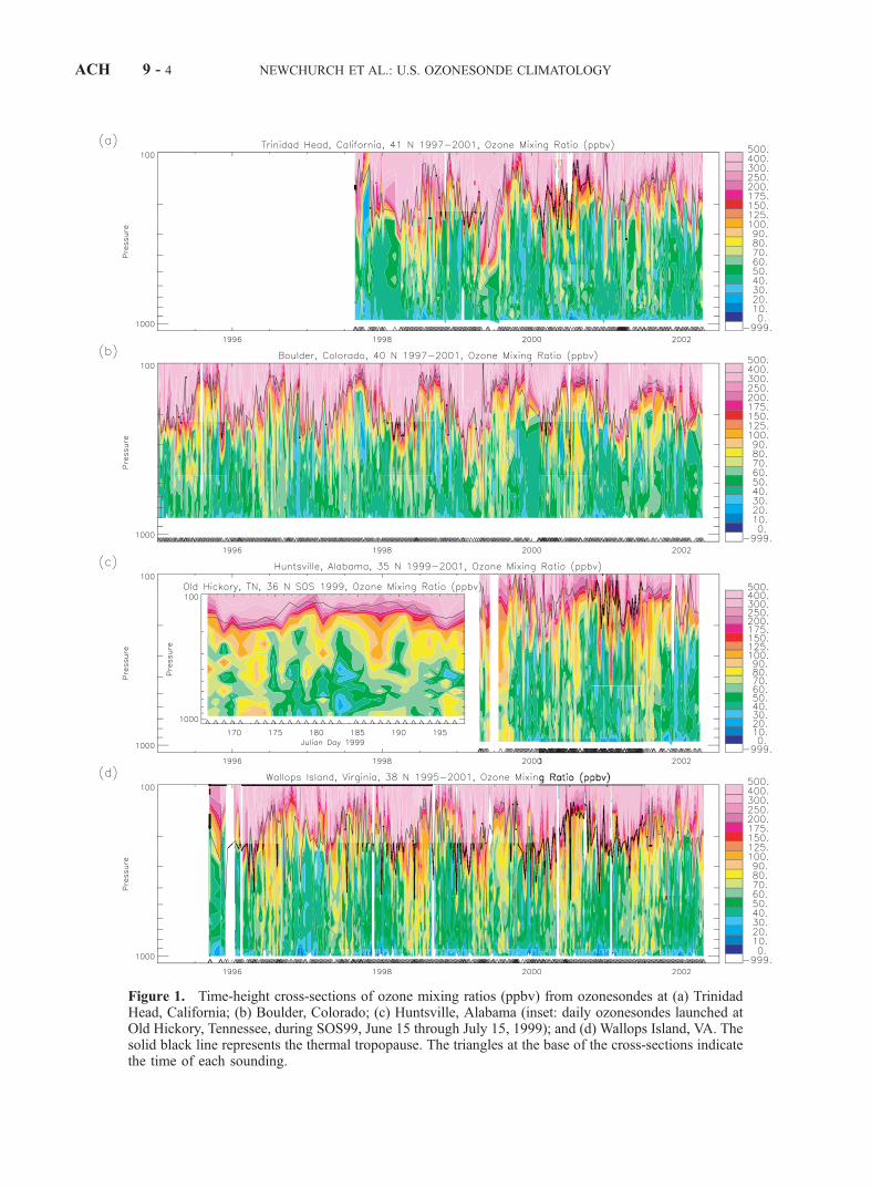
Figure 1. Time-height cross-sections of ozone mixing ratios (ppbv) from ozonesondes at (a) TrinidadHead, California; (b) Boulder, Colorado; (c) Huntsville, Alabama (inset: daily ozonesondes launched atOld Hickory, Tennessee, during SOS99, June 15 through July 15, 1999); and (d) Wallops Island, VA. Thesolid black line represents the thermal tropopause. The triangles at the base of the cross-sections indicatethe time of each sounding.


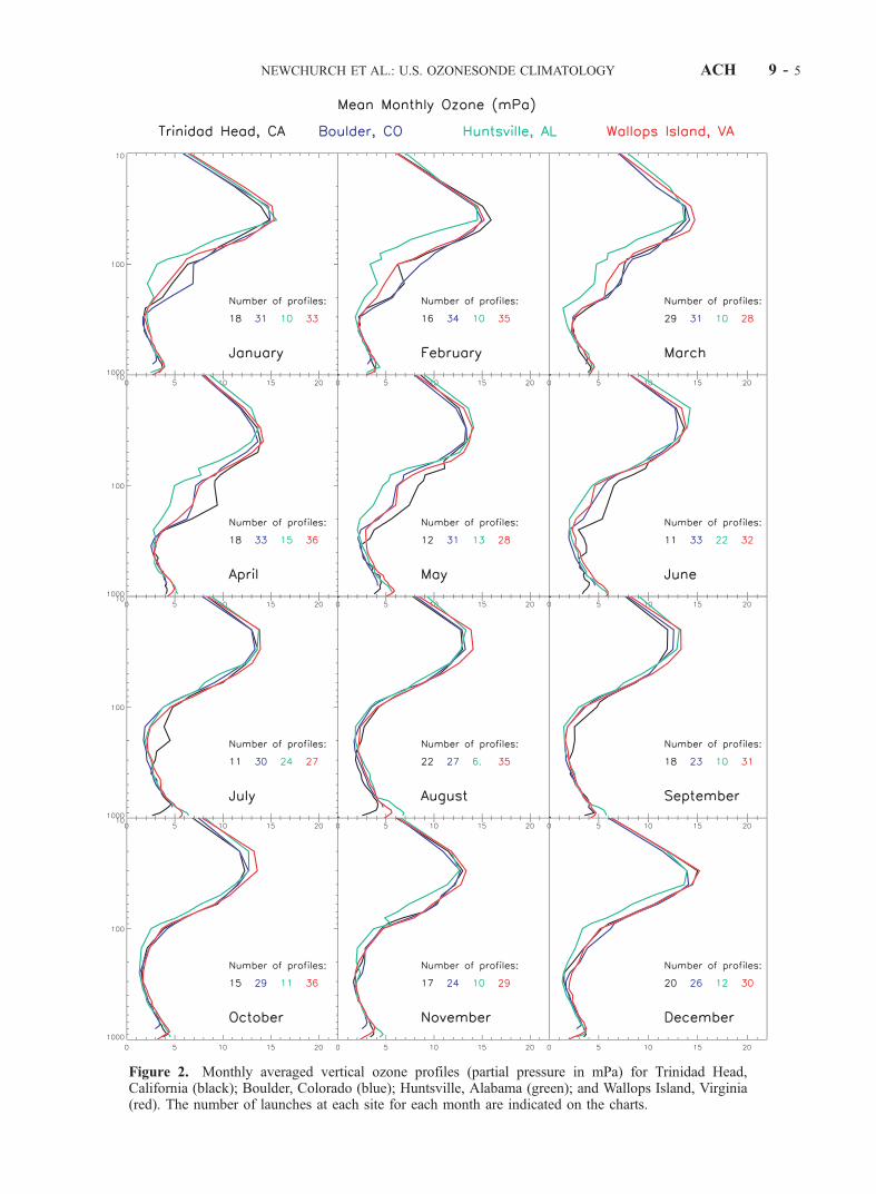
Figure 2. Monthly averaged vertical ozone profiles (partial pressure in mPa) for Trinidad Head,California (black); Boulder, Colorado (blue); Huntsville, Alabama (green); and Wallops Island, Virginia(red). The number of launches at each site for each month are indicated on the charts.


and 3). Below the ozone partial pressure peak, at 50 hPa, thepattern has completely reversed, and ozone concentrationsover Huntsville are lower than at the other three stationsthroughout the year, with the exception of May. This patternholds down to about 200 hPa.[20] The midlatitudes is a region of strong ozone gradients

in the stratosphere. The measured average profiles at the fourstations are consistent with measured/modeled cross-sec-tional analyses of Northern-Hemispheric midlatitude strato-spheric ozone [Cunnold et al., 1975; Logan, 1999a] where achange in the sign of the ozone isopleth gradients occurs ataround 20 hPa. In constructing an emerging ozone climatol-ogy across the United States with data from these fourstations, which all lie within a 6� latitude band, to a firstapproximation, onemight assume that they would belong to asimilar latitudinally dependant regime. However, as shown inFigures 2 and 3, the latitudinal dependence of the altitude ofthe ozone peak at midlatitudes in the stratosphere can bestrong enough to produce significant differences. The lowerlatitude at Huntsville further gives the mean vertical ozoneprofiles characteristics that are more subtropical relative tothe other three stations.[21] The seasonal cycle in the upper stratosphere (10 hPa)

exhibits a broad maximum from early spring through the fall,peaking in June through August for Huntsville and WallopsIsland, May and June for Boulder, and May for TrinidadHead. Between 50–200 hPa, the seasonal cycle in ozonepeaks in early spring through early summer [Logan, 1999a].[22] The lower stratosphere is a region of strong ozone

variability [Fortuin and Kelder, 1998], on both a seasonaland interannual basis. Huntsville displays considerabledifferences in the mean monthly partial pressure ozoneprofiles compared to Trinidad Head, Boulder, and WallopsIsland below 40 hPa. These differences first appear inOctober and intensify throughout the winter, with maximumdifferences in February. Recovering over the spring months,the mean profiles at Huntsville match those at the otherthree stations in the lower stratosphere throughout much ofthe summer (Figures 2 and 3.)[23] Looking at the individual Huntsville profiles for the

three winter periods included in the data set, one can clearlydistinguish a sharp decrease in ozone between the winters of1999/2000 and 2000/2001 between 100–200 hPa. Thisfeature is further highlighted in Figure 4 by the largecoefficient of variation of the monthly mean ozone overHuntsville between 100–200 hPa from November throughMarch. Because the Huntsville data set is only for a 3-yearperiod, the conclusions that can be drawn from the averageprofiles are limited. However, evidence from satellite totalozone analysis at the four stations, combined with averagetotal ozone obtained from the ozonesondes addressed laterin this paper, lends credence to the validity of these averageprofiles in characterizing an emerging ozone profile clima-tology at the four stations.

3.2. Stratosphere-Troposphere Interactions

[24] The annual cycle of the monthly mean ozone mixingratios (ppbv) and the coefficient of variation for the tropo-

Figure 3. (opposite) Monthly average ozone mixing ratios(ppbv) for the four ozonesonde stations at pressure levelsfrom 10 hPa to 800 hPa as indicated on the chart.


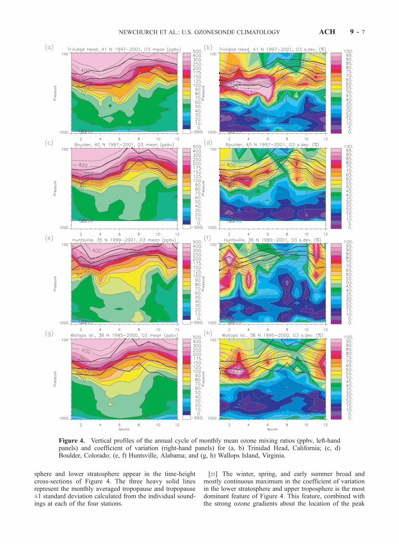
sphere and lower stratosphere appear in the time-heightcross-sections of Figure 4. The three heavy solid linesrepresent the monthly averaged tropopause and tropopause±1 standard deviation calculated from the individual sound-ings at each of the four stations.

[25] The winter, spring, and early summer broad andmostly continuous maximum in the coefficient of variationin the lower stratosphere and upper troposphere is the mostdominant feature of Figure 4. This feature, combined withthe strong ozone gradients about the location of the peak

Figure 4. Vertical profiles of the annual cycle of monthly mean ozone mixing ratios (ppbv, left-handpanels) and coefficient of variation (right-hand panels) for (a, b) Trinidad Head, California; (c, d)Boulder, Colorado; (e, f) Huntsville, Alabama; and (g, h) Wallops Island, Virginia.


coefficient of variation, is indicative of the strong ozonevariability at those altitudes during these months. Thisvariability is consistent with both the seasonal variation inthe height of the tropopause, and the exchange of ozone-richdry air from the stratosphere into the troposphere withintropopause folds associated with strong frontogenesis andcutoff-lows [Cooper et al., 1998; Danielsen, 1968; Holtonet al., 1995; Langford et al., 1996]. Further evidence of thisprocess is in the vertical extent of these enhanced coeffi-cients of variation across the mean tropopause.[26] The coefficients of variation maxima are mostly

below the mean tropopause, where ozone-mixing ratios inthe upper troposphere are usually an order of magnitudesmaller than in the lower stratosphere. The discontinuity inthe high coefficient of variation over Huntsville in March islikely a consequence of the short duration of the data set, inwhich no stratosphere-troposphere exchange (STE) eventswere captured in that month.[27] The Pacific coast station, Trinidad Head, exhibits the

largest cross-tropopause coefficients of variation, along withthe highest average ozone between 100–300 hPa. TrinidadHead also exhibits higher ozone at 300 hPa betweenJanuary and July. This tendency is consistent with a higherfrequency of occurrence of STE episodes within that timeperiod and/or higher intensities of these events in terms ofthe amount of ozone exchanged within the folds relative tothe other three stations. Mean ozone mixing ratios of 100ppbv extend as far down as 400 hPa over Trinidad Head inJune, compared to about 200–250 hPa over the other threestations for the same month.[28] From the magnitude and vertical extent of the

coefficient of variation peaks, a west-to-east gradient isevident in the frequency and/or relative magnitude of theseSTE events and upper free-tropospheric ozone mixingratios. It should be noted at this point that it is very difficultto distinguish between high coefficients of variation causedby STE and the normal variations of the tropopause altitudein the winter and spring months from the monthly averageprofiles. However, for Trinidad Head the coefficient ofvariation maxima extends well below the average tropo-pause plus 1 standard deviation, as does the 125 ppbv ozoneisopleth. This provides further evidence that the elevatedupper tropospheric ozone levels over Trinidad Head are ofstratospheric origin.[29] There is significant interannual variability in ozone

in the upper troposphere/lower stratosphere [Logan, 1994].Comparison of data from the emerging climatology pre-sented here with data from the climatology developed fromaircraft observations [e.g., Marenco et al., 1998; Thouret etal., 1998a, 1998b] for Wallops Island shows good agree-ment with the ozonesonde and MOZAIC data with theexception of the 300 hPa level. There is a noticeabledifference in the structure of the seasonal cycle betweenJanuary and August at 300 hPa for the two ozonesonde datasets. The Wallops Island data set used by [Thouret et al.,1998a] spanned a period from 1980 to 1993. Differencesbetween the average ozone at Wallops Island at 300 hPa canbe attributed to the strong interannual variability in both theheight of the tropopause and the corresponding ozoneconcentrations at 300 hPa and possible changes in instru-mentation/procedures associated with the ozonesondelaunches at Wallops Island.

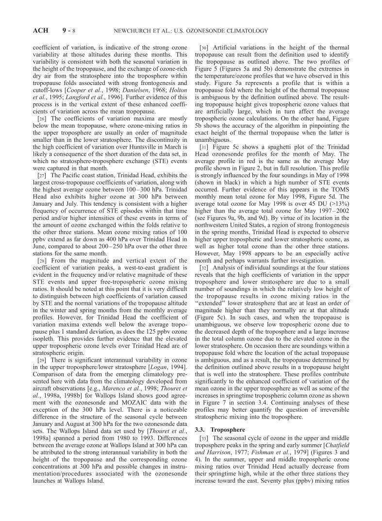
[30] Artificial variations in the height of the thermaltropopause can result from the definition used to identifythe tropopause as outlined above. The two profiles ofFigure 5 (Figures 5a and 5b) demonstrate the extremes inthe temperature/ozone profiles that we have observed in thisstudy. Figure 5a represents a profile that is within atropopause fold where the height of the thermal tropopauseis ambiguous by the definition outlined above. The result-ing tropopause height gives tropospheric ozone values thatare artificially large, which in turn affect the averagetropospheric ozone calculations. On the other hand, Figure5b shows the accuracy of the algorithm in pinpointing theexact height of the thermal tropopause when the latter isunambiguous.[31] Figure 5c shows a spaghetti plot of the Trinidad

Head ozonesonde profiles for the month of May. Theaverage profile in red is the same as the average Mayprofile shown in Figure 2, but in full resolution. This profileis strongly influenced by the four soundings in May of 1998(shown in black) in which a high number of STE eventsoccurred. Further evidence of this appears in the TOMSmonthly mean total ozone for May 1998, Figure 5d. Theaverage total ozone for May 1998 is over 45 DU (>13%)higher than the average total ozone for May 1997–2002(see Figures 9a, 9b, and 9d). By virtue of its location in thenorthwestern United States, a region of strong frontogenesisin the spring months, Trinidad Head is expected to observehigher upper tropospheric and lower stratospheric ozone, aswell as higher total ozone than the other three stations.However, May 1998 appears to be an especially activemonth and perhaps warrants further investigation.[32] Analysis of individual soundings at the four stations

reveals that the high coefficients of variation in the uppertroposphere and lower stratosphere are due to a smallnumber of soundings in which the relatively low height ofthe tropopause results in ozone mixing ratios in the‘‘extended’’ lower stratosphere that are at least an order ofmagnitude higher than they normally are at that altitude(Figure 5c). In such cases, and when the tropopause isunambiguous, we observe low tropospheric ozone due tothe decreased depth of the troposphere and a large increasein the total column ozone due to the elevated ozone in thelower stratosphere. On occasion there are soundings within atropopause fold where the location of the actual tropopauseis ambiguous, and as a result, the tropopause determined bythe definition outlined above results in a tropopause heightthat is well into the stratosphere. These profiles contributesignificantly to the enhanced coefficient of variation of themean ozone in the upper troposphere as well as some of theincreases in springtime tropospheric column ozone as shownin Figure 7 in section 3.4. Continuing analyses of theseprofiles may better quantify the question of irreversiblestratospheric mixing into the troposphere.

3.3. Troposphere

[33] The seasonal cycle of ozone in the upper and middletroposphere peaks in the spring and early summer [Chatfieldand Harrison, 1977; Fishman et al., 1979] (Figures 3 and4). In the summer, upper and middle tropospheric ozonemixing ratios over Trinidad Head actually decrease fromtheir springtime high, while at the other three stations theyincrease toward the east. Seventy plus (ppbv) mixing ratios


extend as far down as 400 hPa over Boulder and 500–550hPa over Huntsville and Wallops Island.[34] Although they decrease substantially during the sum-

mer, the ozone coefficients of variation in the upper tropo-sphere remain notable (40–70%). The summer coefficientof variation maximum is located almost entirely below theaverage tropopause, with a large gradient at the tropopause,highlighting the substantial week-to-week variability in theupper troposphere, as well as completely decoupling thisvariability from local stratospheric influences. Possiblesources of this variability include transport of ozone pre-viously exchanged into the upper troposphere at higherlatitudes and/or en route photochemical production ofozone. [Chatfield and Delany, 1990] refer to a mechanismthey call ‘‘mix-then-cook,’’ in which vertical redistributionof ozone precursors by convection and subsequent transportcan result in enhanced photochemical production of ozone

and elevated middle and upper tropospheric ozone concen-trations [Dickerson et al., 1987; Ellis et al., 1996; Liu et al.,1987; Pickering et al., 1989, 1992, 1990; Thompson et al.,1994]. In a back-trajectory case study analysis of ozone-sonde measurements, we also have observed evidence ofthis phenomenon during SOS99 in Nashville, TN (notshown).[35] The amplitude of the seasonal cycle of ozone

reaches a minimum in the middle troposphere at 500 hPa[Logan, 1985]. Coefficients of variation throughout theentire year and for all four stations show broad minimaacross the middle and lower free troposphere (about 500–800 hPa) (Figure 4). Of significance from the contour plotof mean ozone and standard deviations is the shape of thelower and middle-tropospheric mean ozone curves at thefour stations. Boulder, Huntsville, and Wallops Island allshow similar shapes of the annual cycle of the mean ozone,

Figure 5. Individual soundings (a, b) from Wallops Island that demonstrate the extremes in lapse ratestructure used to determine the height of the tropopause given the definition in the text and its effect onthe computed tropospheric ozone. (c) Spaghetti plot of the nine Trinidad Head soundings in the month ofMay for the study period. The black profiles (4) are in 1998, the blue (1) is in 1999, the green (4) are in2000, the magenta (3) are in 2001, and the red is the average profile. (d) Monthly mean total ozone fromTOMS for May 1998. The blue diamonds mark the locations of the four ozonesonde stations.


differing only in the relative amplitudes of the cycle.Trinidad Head exhibits a rather different cycle in the annualmean ozone in the lower and middle troposphere, suggest-ing that the processes that govern ozone concentrations atTrinidad Head are different from those at the other threelocations.[36] In the lower troposphere, the seasonal cycle of ozone

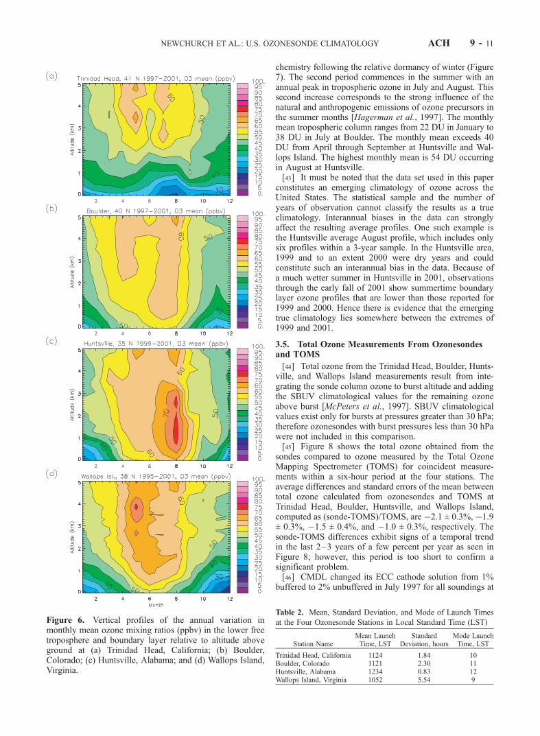
peaks in the summer months [Logan, 1985]. Little variationin the ozone cycle occurs in the lower troposphere overTrinidad Head; however, the seasonal signature is verystrong over Huntsville and Wallops Island and is moderateover Boulder. Over Huntsville, ozone concentrations thatexceed the mean of the other three stations by as much as25–30% at 700 and 800 hPa in August, and 800 hPa inSeptember (Figure 3) are clearly evident. However, theHuntsville August data is an average of only six profileswithin a three year period, such a sparse record limits theconclusions that can be drawn from them. Within theplanetary boundary layer, a steady increase in ozone mixingratios during the summer months is evident at Boulder,Huntsville, and Wallops Island, but Trinidad Head exhibits apronounced decrease in boundary layer ozone mixing ratiosduring the summer (Figure 6). At Huntsville, the summerpeak in ozone extends from the surface to about 3 km (650hPa) with a strong, well-mixed maximum in August of 70+ppbv, and a notable gradient immediately above the con-vective boundary layer (CBL).[37] Throughout the summer in the lower troposphere

over Huntsville, ozone-mixing ratios are largest near thesurface and decrease upward, suggesting a surface sourcefor the elevated ozone. These surface sources could beaccounted for by increased summertime natural emissionsof isoprene from deciduous trees in the southeastern UnitedStates as well as other nonmethane hydrocarbons [Andron-ache et al., 1994; Doskey and Gao, 1999; Hagerman et al.,1997; Liang et al., 1998; Nouaime et al., 1998; Sillman etal., 1995; Starn et al., 1998]. Boundary layer ozone levels atthe other three sites do not show maxima at the surface,especially at the two coastal sites, Trinidad Head andWallops Island. There is a local minimum in ozone mixingratios in a 1 km layer extending above the surface overTrinidad Head during July and August. This feature resultsin a summertime minimum in surface ozone at TrinidadHead, in contrast to the other three stations, further suggest-ing that the ozone source in that region is not from thesurface and not local. The summer minimum could beaccounted for by a shallow sea breeze coupled with thepredominantly westerly flow that brings in clean air fromthe Pacific during the day and whose intensity is maximizedin the summer when differential surface heating betweenland and water is greatest.[38] Boundary layer ozone exhibits a larger diurnal

signature than does ozone in the free troposphere, hencesensitivity to the average time at which the ozonesondesfly is higher in the boundary layer. Table 2 shows themean, standard deviation, and mode of the launch timesfor the four stations in local standard time (LST). ForWallops Island, the large standard deviation of the meanlaunch time indicates that the sample represents an aver-age over the entire day, which in turn would result in alower average ozone profile for the boundary layer thanwould the mid-afternoon launches at Huntsville (standard

deviation less than 1 hour,) and the other two stations aswell.

3.4. Integrated Tropospheric Ozone

[39] Integrating the column ozone from the ground to thetropopause using data from the ozonesondes provides anaccurate measure of the tropospheric ozone column. Figure7 shows the tropospheric ozone columns for the fourstations over the data period, along with the annual cycleof the monthly average tropospheric column ozone for eachstation. The figure shows a pronounced seasonal cycle inaverage tropospheric column ozone for Boulder, Huntsville,and Wallops Island, with increases in tropospheric ozonebeginning early in the spring, and maxima well into thesummer months. Trinidad Head, on the other hand, does notdisplay the same structure apparent at the other threestations. There is an increase in tropospheric ozone in theearly spring, but there is no such corresponding increasethrough the summer months. The magnitudes of the averagetropospheric columns differ from station to station withpeaks at or above 50 DU for Huntsville in July and Augustand for Wallops Island in May through July. The largeststandard deviations of the monthly average troposphericozone column are in the spring and fall at all four stations.[40] The increase in tropospheric column ozone in the

summer is due to two main factors: an increase in thephotochemical production of ozone, and a correspondingincrease in the height of the average tropopause. Analysis ofthe seasonal variation in the height of the monthly averagedtropopause from Figure 4 shows the larger amplitudes overthe two inland sites, Huntsville and Boulder, and smalleramplitudes for the seasonal cycle over the coastal stations,Trinidad Head and Wallops Island. The amplitude of theseasonal cycle in the height of the tropopause will tend toimpose a dynamical, or nonphotochemical, effect on theincreased tropospheric ozone columns observed during thesummer months; however, a major contribution remainsfrom the photochemistry.[41] The dash-dotted lines in Figure 7 represent the height

of the monthly averaged tropopause. The dashed linesrepresent the monthly average tropospheric ozone in (DU/km) � 10. Analysis of the annual cycle of integratedtropospheric ozone per km at all four stations shows aninitial peak in April or May, reflecting the role of dynamicaleffects such as STE in modulating tropospheric ozone. AtTrinidad Head, tropospheric ozone concentrations of over 3DU/km are maintained through July, and they decrease withincreases in tropopause height through the remainder of thesummer and into fall and winter. Boulder and WallopsIsland display similar slow decreases in tropospheric ozoneconcentrations through August; however, Wallops Islandconcentrations are about 40–50% higher than those atBoulder. Huntsville, on the other hand, displays a uniquecharacteristic in its gradually increasing tropospheric ozoneconcentrations, which show a secondary peak of 3.5 DU/kmin August. This difference from the other stations is due tothe very high ozone mixing ratios observed in the boundarylayer and upper troposphere over Huntsville (Figure 6).[42] Boulder, Huntsville, and Wallops Island experience

two periods of increasing tropospheric ozone. The firstincrease occurs in early spring as a result of stratosphere-troposphere exchange, and likely the initiation of photo-


chemistry following the relative dormancy of winter (Figure7). The second period commences in the summer with anannual peak in tropospheric ozone in July and August. Thissecond increase corresponds to the strong influence of thenatural and anthropogenic emissions of ozone precursors inthe summer months [Hagerman et al., 1997]. The monthlymean tropospheric column ranges from 22 DU in January to38 DU in July at Boulder. The monthly mean exceeds 40DU from April through September at Huntsville and Wal-lops Island. The highest monthly mean is 54 DU occurringin August at Huntsville.[43] It must be noted that the data set used in this paper

constitutes an emerging climatology of ozone across theUnited States. The statistical sample and the number ofyears of observation cannot classify the results as a trueclimatology. Interannual biases in the data can stronglyaffect the resulting average profiles. One such example isthe Huntsville average August profile, which includes onlysix profiles within a 3-year sample. In the Huntsville area,1999 and to an extent 2000 were dry years and couldconstitute such an interannual bias in the data. Because ofa much wetter summer in Huntsville in 2001, observationsthrough the early fall of 2001 show summertime boundarylayer ozone profiles that are lower than those reported for1999 and 2000. Hence there is evidence that the emergingtrue climatology lies somewhere between the extremes of1999 and 2001.

3.5. Total Ozone Measurements From Ozonesondesand TOMS

[44] Total ozone from the Trinidad Head, Boulder, Hunts-ville, and Wallops Island measurements result from inte-grating the sonde column ozone to burst altitude and addingthe SBUV climatological values for the remaining ozoneabove burst [McPeters et al., 1997]. SBUV climatologicalvalues exist only for bursts at pressures greater than 30 hPa;therefore ozonesondes with burst pressures less than 30 hPawere not included in this comparison.[45] Figure 8 shows the total ozone obtained from the

sondes compared to ozone measured by the Total OzoneMapping Spectrometer (TOMS) for coincident measure-ments within a six-hour period at the four stations. Theaverage differences and standard errors of the mean betweentotal ozone calculated from ozonesondes and TOMS atTrinidad Head, Boulder, Huntsville, and Wallops Island,computed as (sonde-TOMS)/TOMS, are �2.1 ± 0.3%, �1.9± 0.3%, �1.5 ± 0.4%, and �1.0 ± 0.3%, respectively. Thesonde-TOMS differences exhibit signs of a temporal trendin the last 2–3 years of a few percent per year as seen inFigure 8; however, this period is too short to confirm asignificant problem.[46] CMDL changed its ECC cathode solution from 1%

buffered to 2% unbuffered in July 1997 for all soundings at

Figure 6. Vertical profiles of the annual variation inmonthly mean ozone mixing ratios (ppbv) in the lower freetroposphere and boundary layer relative to altitude aboveground at (a) Trinidad Head, California; (b) Boulder,Colorado; (c) Huntsville, Alabama; and (d) Wallops Island,Virginia.

Table 2. Mean, Standard Deviation, and Mode of Launch Times

at the Four Ozonesonde Stations in Local Standard Time (LST)

Station NameMean LaunchTime, LST

StandardDeviation, hours

Mode LaunchTime, LST

Trinidad Head, California 1124 1.84 10Boulder, Colorado 1121 2.30 11Huntsville, Alabama 1234 0.83 12Wallops Island, Virginia 1052 5.54 9


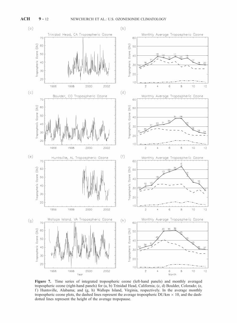
Figure 7. Time series of integrated tropospheric ozone (left-hand panels) and monthly averagedtropospheric ozone (right-hand panels) for (a, b) Trinidad Head, California; (c, d) Boulder, Colorado; (e,f ) Huntsville, Alabama; and (g, h) Wallops Island, Virginia, respectively. In the average monthlytropospheric ozone plots, the dashed lines represent the average tropospheric DU/km � 10, and the dash-dotted lines represent the height of the average tropopause.


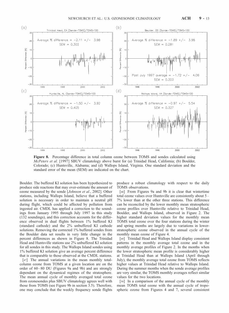
Boulder. The buffered KI solution has been hypothesized toproduce side reactions that may over-estimate the amount ofozone measured by the sonde [Johnson et al., 2002]. Otherstations, including Wallops Island, believe that a bufferedsolution is necessary in order to maintain a neutral pHduring flight, which could be affected by pollution fromingested air. CMDL has applied a correction to the sound-ings from January 1995 through July 1997 in this study(132 soundings), and this correction accounts for the differ-ence observed in dual flights between 1% buffered KI(standard cathode) and the 2% unbuffered KI cathodesolutions. Removing the corrected 1% buffered sondes fromthe Boulder data set results in very little change in thepercent differences as shown in Figure 8. The TrinidadHead and Huntsville stations use 2% unbuffered KI solutionfor all sondes in this study. The Wallops Island sondes using1% buffered KI solution give an average percent differencethat is comparable to those observed at the CMDL stations.[47] The annual variations in the mean monthly total-

column ozone from TOMS at a given location are on theorder of 60–80 DU (Figures 9a and 9b) and are stronglydependant on the dynamical regimes of the stratosphere.The mean annual cycle of monthly averaged total ozonefrom ozonesondes plus SBUV climatology agrees well withthose from TOMS (see Figure 9b in section 3.5). Therefore,one may conclude that the weekly frequency sonde flights

produce a robust climatology with respect to the dailyTOMS observations.[48] From Figures 9a and 9b it is clear that wintertime

total ozone values over Huntsville are consistently about 5–7% lower than at the other three stations. This differencecan be reconciled by the lower monthly mean stratosphericozone profiles over Huntsville relative to Trinidad Head,Boulder, and Wallops Island, observed in Figure 2. Thehigher standard deviation values for the monthly meanTOMS total ozone over the four stations during the winterand spring months are largely due to variations in lower-stratospheric ozone observed in the annual cycle of themonthly mean ozone of Figure 4.[49] Trinidad Head and Wallops Island display consistent

patterns in the monthly average total ozone and in themonthly average profiles of Figure 2. In the months whenthe lower stratospheric mean profile is considerably higherat Trinidad Head than at Wallops Island (April throughJuly), the monthly average total ozone from TOMS reflectshigher values at Trinidad Head relative to Wallops Island.During the summer months when the sonde average profilesare very similar, the TOMS monthly averages reflect similarvalues for the two locations.[50] In a comparison of the annual cycle of the monthly

mean TOMS total ozone with the annual cycle of tropo-spheric ozone from Figures 4 and 7, several consistent

Figure 8. Percentage difference in total column ozone between TOMS and sondes calculated usingMcPeters et al. [1997] SBUV climatology above burst for (a) Trinidad Head, California; (b) Boulder,Colorado; (c) Huntsville, Alabama; and (d) Wallops Island, Virginia. One standard deviation and thestandard error of the mean (SEM) are indicated on the chart.


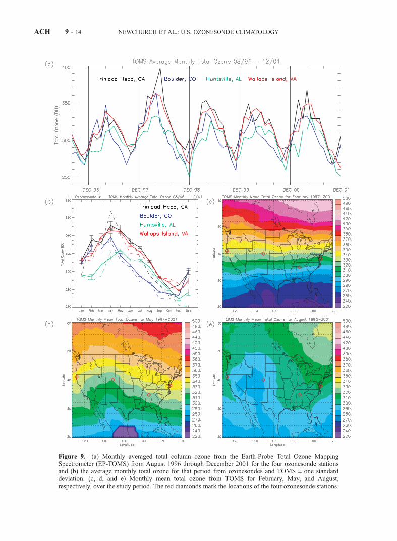
Figure 9. (a) Monthly averaged total column ozone from the Earth-Probe Total Ozone MappingSpectrometer (EP-TOMS) from August 1996 through December 2001 for the four ozonesonde stationsand (b) the average monthly total ozone for that period from ozonesondes and TOMS ± one standarddeviation. (c, d, and e) Monthly mean total ozone from TOMS for February, May, and August,respectively, over the study period. The red diamonds mark the locations of the four ozonesonde stations.


features appear: (1) The peak in the monthly average TOMStotal ozone over Trinidad Head between April and July(Figure 9) corresponds with the peak in lower-strato-spheric/upper-tropospheric ozone over Trinidad Head rela-tive to the other three stations (Figures 2, 3, and 4). (2)Although the annual variations of the total ozone columnover Trinidad Head andWallops Island are similar (Figure 9),the partitioning between tropospheric and stratospheric por-tions (Figures 4 and 6) changes over the year. (3) TheHuntsville total column is the lowest of the four stationsfrom December through April (Figures 9b and 9c) because ofsmaller ozone amounts in the lower stratosphere (Figure 2).(4) The decrease in total ozone at Boulder relative to Hunts-ville from May through October (Figures 9b and 9e) resultsfrom a combination of differences in altitude (about 5 DU)and a persistent planetary wave during the summer months inthe stratosphere. This waveforms a feature of low ozone(about 15 DU) over the western plains of the United States(Figure 9).

3.6. Variations Across the Continental United States

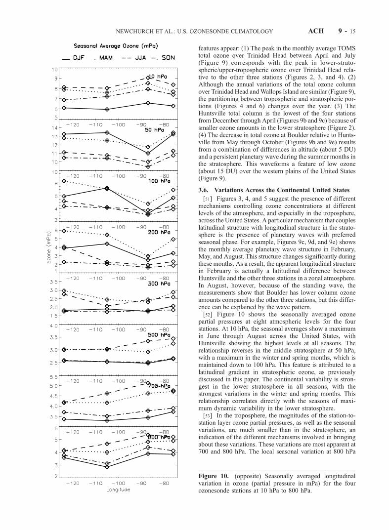
[51] Figures 3, 4, and 5 suggest the presence of differentmechanisms controlling ozone concentrations at differentlevels of the atmosphere, and especially in the troposphere,across the United States. A particular mechanism that coupleslatitudinal structure with longitudinal structure in the strato-sphere is the presence of planetary waves with preferredseasonal phase. For example, Figures 9c, 9d, and 9e) showsthe monthly average planetary wave structure in February,May, and August. This structure changes significantly duringthese months. As a result, the apparent longitudinal structurein February is actually a latitudinal difference betweenHuntsville and the other three stations in a zonal atmosphere.In August, however, because of the standing wave, themeasurements show that Boulder has lower column ozoneamounts compared to the other three stations, but this differ-ence can be explained by the wave pattern.[52] Figure 10 shows the seasonally averaged ozone

partial pressures at eight atmospheric levels for the fourstations. At 10 hPa, the seasonal averages show a maximumin June through August across the United States, withHuntsville showing the highest levels at all seasons. Therelationship reverses in the middle stratosphere at 50 hPa,with a maximum in the winter and spring months, which ismaintained down to 100 hPa. This feature is attributed to alatitudinal gradient in stratospheric ozone, as previouslydiscussed in this paper. The continental variability is stron-gest in the lower stratosphere in all seasons, with thestrongest variations in the winter and spring months. Thisrelationship correlates directly with the seasons of maxi-mum dynamic variability in the lower stratosphere.[53] In the troposphere, the magnitudes of the station-to-

station layer ozone partial pressures, as well as the seasonalvariations, are much smaller than in the stratosphere, anindication of the different mechanisms involved in bringingabout these variations. These variations are most apparent at700 and 800 hPa. The local seasonal variation at 800 hPa

Figure 10. (opposite) Seasonally averaged longitudinalvariation in ozone (partial pressure in mPa) for the fourozonesonde stations at 10 hPa to 800 hPa.


over Trinidad Head is the smallest of the four stations aswell as the smallest for all atmospheric levels considered.Average ozone partial pressures for Trinidad Head from thesurface to 500 hPa vary by less than 1 mPa over the entireyear, with a minimum over the fall and winter months and amaximum over the spring and summer months. The magni-tude of this seasonal variation at Trinidad Head providesfurther evidence that the ozone sources in the northwesternUnited States are primarily nonlocal. In the lower freetroposphere (500–800 hPa in Figure 10), and within theplanetary boundary layer a west-to-east increasing gradientin ozone is clearly discernable, however, particularly in thelower levels, we speculate that these increases are morelikely attributable to local pollution effects than a longitu-dinal gradient across the United States.

4. Conclusions

[54] As a result of several years of ozonesonde measure-ments at four locations in the United States, a climatologyof the vertical profile of continental U.S. ozone is beginningto emerge. This vertical distribution of ozone displayssignificant variation on timescales ranging from days tointerannual in both intrastation and interstation observa-tions. The records show strong evidence of stratosphere-troposphere exchange, especially in the winter and spring,and more so at the Pacific coast station, Trinidad Head. Allstations show variability in the boundary layer pollutionsources. The middle troposphere is the least variable region.The variability throughout the troposphere and lower strato-sphere is quantified by coefficients of variation of themonthly means showing strong vertical and seasonal struc-ture. Even with this strong variability, comparison toMOZAIC aircraft measurements shows good agreement,except at 300 hPa, which may be attributed to stronginterannual variability between the data sets.[55] In the lower troposphere, the two eastern stations,

Huntsville, Alabama, and Wallops Island, Virginia, measurethe highest ozone amounts compared to the two westernstations, Trinidad Head, California, and Boulder, Colorado.The lower stratospheric ozone at Huntsville, Alabama, isnoticeably lower on average than at the other three stationsin the winter and springtime. All stations show very strongvariability in this altitude region, especially in winter andspringtime. During extreme events, stratospheric peakozone partial pressures pervade the troposphere down to500 hPa. Throughout the stratosphere, the Huntsville pro-files display more tropical character than the other threestations, a distinction most noticeable during winter andspring.[56] In comparing the seasonal signature of ozone across

the United States, eastern stations exhibit higher troposphericozone concentrations as a result of local pollution effects. Theseasonal cycle maximizes in the summer months at allstations except at Trinidad Head, which has the oppositephase. Huntsville experiences the highest ozone mixingratios in the summertime convective boundary layer, reach-ing 75 ppbv on average in August. The other three sitesexperience significant vertical gradients in volume mixingratio in the lowest �1 km with surface minima.[57] Boulder, Huntsville, and Wallops Island stations

show a pronounced seasonal cycle in integrated tropo-

spheric ozone maximizing in the summer; the amplitudeat Trinidad Head is significantly smaller. Wintertime min-ima range from 25 DU at Boulder to 30 DU at WallopsIsland. Huntsville and Wallops Island experience the largesttropospheric column ozone amounts (>50 DU); TrinidadHead and Boulder both peak at �40 DU. These summer-time maxima result from both higher mixing ratios and ahigher tropopause. The signatures of stratosphere-tropo-sphere exchange and photochemical production are bothevident in the column effects.[58] The sonde-TOMS average differences in total ozone

column range from �1% to �2% with some indication of apositive secular change in that bias. The seasonal characterof TOMS column ozone at the sonde locations is consistentwith the sonde-plus-SBUV-climatology total columns.Therefore, inspecting the sonde variations within the spa-tial/temporal context of the TOMS-measured ozone mor-phology reveals preferred wave patterns in the ozone fieldthat result in the observed ozone profiles and the couplingbetween latitude and longitude effects, which vary withaltitude.

[59] Acknowledgments. We would like to acknowledge J. Logan forher insightful comments and Tom Northam/WFF for assistance with theWFF data. This research was supported by the NOAA Health of theAtmosphere Program, the NASA Atmospheric Chemistry Modeling andAnalysis Program.

ReferencesAndronache, C., W. L. Chameides, M. O. Rodgers, J. Martinez, P. Zimmer-man, and J. Greenberg, Vertical distribution of isoprene in the lowerboundary layer of the rural and urban southern United States, J. Geophys.Res., 99, 16,989–16,999, 1994.

Attmannspacher, W., J. de la Noe, D. de Muer, J. Lenoble, G. Megie, J.Pelon, P. Pruvost, and R. Reiter, European validation of SAGE II ozoneprofiles, J. Geophys. Res., 94, 8461–8466, 1989.

Beekmann, M., G. Ancellet, and G. Megie, Climatology of troposphericozone in the southern Europe and its relation to potential vorticity,J. Geophys. Res., 99, 12,841–12,853, 1994.

Bethan, S., G. Vaughan, and S. J. Reid, A comparison of ozone and thermaltropopause heights and the impact of tropopause definition on quantify-ing the ozone content of the troposphere, Q. J. R. Meteorol. Soc., 122,929–944, 1996.

Bodecker, G. E., I. S. Boyd, and W. A. Matthews, Trends and variability invertical ozone and temperature profiles measured by ozonesondes atLauder, New Zealand: 1986–1996, J. Geophys. Res., 103, 28,661–28,681, 1998.

Brinksma, E. J., et al., Validation of 3 years of ozone measurements overNetwork for the Detection of Stratospheric Change station Lauder, NewZealand, J. Geophys. Res., 105, 17,291–17,306, 2000.

Chameides, W. L., et al., Ozone precursor relationships in the ambientatmosphere, J. Geophys. Res., 97, 6037–6055, 1992.

Chatfield, R. B., and A. C. Delany, Convection links biomass burning toincreased tropical ozone, however, models will typically over-predict O3,J. Geophys. Res., 95, 18,473–18,488, 1990.

Chatfield, R., and H. Harrison, Tropospheric ozone, 1, Evidence for higherbackground values, J. Geophys. Res., 82, 5964–5968, 1977.

Cooper, O. R., J. L. Moody, J. C. Davenport, S. J. Oltmans, B. J. Johnson,X. Chen, P. B. Shepson, and J. T. Merrill, Influence of springtime weathersystems on vertical ozone distributions over three North American sites,J. Geophys. Res., 103, 22,001–22,013, 1998.

Cunnold, D., F. Alyea, N. Phillips, and R. Prinn, A three-dimensionaldynamical-chemical model of atmospheric ozone, J. Atmos. Sci., 32,170–194, 1975.

Cunnold, D. M., W. P. Chu, R. A. Barnes, M. P. McCormick, and R. E.Veiga, Validation of SAGE II ozone measurements, J. Geophys. Res., 94,8447–8460, 1989.

Danielsen, E. F., The laminar structure of the tropopause and its relation tothe concept of the tropopause, Arch. Meteorol. Geophys. Bioklimatol.,BII, 293–332, 1959.

Danielsen, E. F., Stratosphere-troposphere exchange based on radioactivity,ozone and potential vorticity, J. Atmos. Sci., 25, 502–518, 1968.


Dickerson, R. R., et al., Thunderstorms: An important mechanism in thetransport of air pollutants, Science, 235, 460–465, 1987.

Doskey, P. V., and W. Gao, Vertical mixing and chemistry of isoprene in theatmospheric boundary layer: Aircraft-based measurements and numericalmodeling, J. Geophys. Res., 104, 21,263–21,274, 1999.

Ellis, W. G., Jr., A. M. Thompson, S. Kondragunta, K. E. Pickering, G.Stenchikov, R. R. Dickerson, and W. K. Tao, Potential ozone productionfollowing convective transport based on future emission scenarios, At-mos. Environ., 30, 667–672, 1996.

Fishman, J., V. Ramanathan, P. J. Crutzen, and S. C. Liu, Troposphericozone and climate, Nature, 282, 818–820, 1979.

Fortuin, J. P. F., and H. Kelder, An ozone climatology based on ozonesondeand satellite measurements, J. Geophys. Res., 103, 31,709–31,734, 1998.

Frost, G. J., et al., Photochemical ozone production in the rural southeasternUnited States during the 1990 Rural Oxidants in the Southern Environ-ment (ROSE) program, J. Geophys. Res., 103, 22,491–22,508, 1998.

Hagerman, L. M., V. P. Aneja, and W. A. Lonneman, Characterization ofnon-methane hydrocarbons in the rural southeast United States, Atmos.Environ., 31, 4017–4038, 1997.

Holton, J. R., P. H. Haynes, M. E. McIntyre, A. R. Douglass, R. B. Rood,and L. Pfister, Stratosphere-troposphere exchange, Rev. Geophys, 33,403–439, 1995.

Hoogen, R., V. V. Rozanov, and J. P. Burrows, Ozone profiles from GOMEsatellite data: Algorithm description and first validation, J. Geophys. Res.,104, 8263–8280, 1999.

Johnson, B. J., S. J. Oltmans, H. Vomel, T. Deshler, and C. Kroger, Elec-trochemical concentration cell (ECC) ozonesonde pump efficiency mea-surements and tests on the sensitivity to ozone of buffered and unbufferedECC sensor cathode solutions, J. Geophys. Res., 107, 4393, doi:10.1029/2001JD000557, 2002.

Kalnay, E., et al., The NCEP/NCAR 40-year reanalysis project, Bull. Am.Meteorol. Soc., 77, 437–471, 1996.

Kim, J. H., M. J. Newchurch, and K. Han, Distribution of Tropical tropo-spheric ozone determined by the scan-angle method applied to TOMSmeasurements, J. Atmos. Sci., 58, 2699–2708, 2001.

Komhyr, W. D., Electrochemical cells for gas analysis, Ann. Geophys., 25,203–210, 1969.

Komhyr, W. D., R. A. Barnes, G. B. Brothers, J. A. Lanthrop, and D. P.Opperman, Electrochemical concentration cell ozonesonde performanceevaluation during STOIC 1989, J. Geophys. Res., 100, 9231–9244,1995.

Langford, A. O., C. D. Masters, M. H. Proffitt, E.-Y. Hsie, and A. F. Tuck,Ozone measurements in a tropopause fold associated with a cut-off lowsystem, Geophys. Res. Lett., 23, 2501–2504, 1996.

Liang, J., L. W. Horowitz, D. J. Jacob, Y. Wang, A. M. Fiore, J. A. Logan,G. M. Gardner, and J. W. Munger, Seasonal budgets of reactive nitrogenspecies and ozone over the United States, and export fluxes to the globalatmosphere, J. Geophys. Res., 103, 13,435–13,450, 1998.

Liu, S. C., M. Trainer, F. C. Fehsenfeld, D. D. Parrish, E. J. Williams, D. W.Fahey, G. Hubler, and P. C. Murphy, Ozone production in the rural tropo-sphere and the implications for regional and global ozone distributions,J. Geophys. Res., 92, 4191–4207, 1987.

Logan, J. A., Tropospheric ozone: Seasonal behavior, trends, and anthro-pogenic influence, J. Geophys. Res., 90, 10,463–10,482, 1985.

Logan, J. A., Trends in the vertical distribution of ozone: An analysis ofozonesonde data, J. Geophys. Res., 99, 25,553–25,585, 1994.

Logan, J. A., An analysis of ozonesonde data for the lower stratosphere:Recommendations for testing models, J. Geophys. Res., 104, 16,151–16,170, 1999a.

Logan, J. A., An analysis of ozonesonde data for the troposphere: Recom-mendations for testing 3-D models and development of a gridded clima-tology for tropospheric ozone, J. Geophys. Res., 104, 16,115–16,149,1999b.

Lucke, R. L., et al., The Polar Ozone and Aerosol Measurement (POAM)III instrument and early validation results, J. Geophys. Res., 104,18,785–18,799, 1999.

Marenco, A., et al., Measurement of ozone and water vapor by Airbus in-service aircraft: The MOZAIC airborne program, An overview, J. Geo-phys. Res., 103, 25,631–25,642, 1998.

Margitan, J. J., et al., Stratospheric Ozone Intercomparisons Campaigns(STOIC) 1989: Overview, J. Geophys. Res., 100, 9193–9207, 1995.

McPeters, R. D., G. J. Labow, and B. J. Johnson, A satellite-derived ozoneclimatology for balloonsonde estimation of total column ozone, J. Geo-phys. Res., 102, 8875–8885, 1997.

Montzka, S. A., M. Trainer, P. D. Goldan, W. C. Kuster, and F. C.Fehsenfeld, Isoprene and its oxidation products, methyl vinyl ketoneand methacrolein, in the rural troposphere, J. Geophys. Res., 98, 1101–1111, 1993.

Newchurch, M. J., X. Liu, and J. H. Kim, Lower Tropospheric Ozone(LTO) derived from TOMS near mountainous regions, J. Geophys.Res., 106, 20,403–20,412, 2001a.

Newchurch, M. J., X. Liu, J. H. Kim, and P. K. Bhartia, On the accuracy ofTOMS retrievals over cloudy regions, J. Geophys. Res., 106, 32,315–32,326, 2001b.

Nouaime, G., S. B. Bertman, C. Seaver, D. Elyea, H. Huang, P. B. Shepson,T. K. Starn, D. D. Riemer, R. G. Zika, and K. Olszyna, Sequentialoxidation products from tropospheric isoprene chemistry: MACR andMPAN at a NOx-rich forest environment in the southeastern UnitedStates, J. Geophys. Res., 103, 22,463–22,471, 1998.

Oltmans, S. J., et al., Summer and spring ozone profiles over the NorthAtlantic from ozonesonde measurements, J. Geophys. Res., 101, 29,179–29,200, 1996.

Pickering, K. E., R. R. Dickerson, W. T. Luke, and L. J. Nunnermacker,Clear-sky vertical profiles of trace gases as influenced by upstream con-vective activity, J. Geophys. Res., 94, 14,879–14,892, 1989.

Pickering, K. E., A. M. Thompson, R. R. Dickerson, W. T. Luke, D. P.McNamara, J. P. Greenberg, and P. R. Zimmerman, Model calculations oftropospheric ozone production potential following observed convectiveevents, J. Geophys. Res., 95, 14,049–14,062, 1990.

Pickering, K. E., A. Thompson, J. R. Scala, W.-K. Tao, R. Dickerson, andJ. Simpson, Free tropospheric ozone production following entrainment ofurban plumes into deep convection, J. Geophys. Res., 97, 17,985–18,000, 1992.

Reid, S. J., G. Vaughan, A. R. W. Marsh, and H. G. J. Smit, Accuracy ofozonesonde measurements in the troposphere, J. Atmos. Chem., 25, 215–236, 1996.

Reiter, E. R., M. E. Glasser, and J. D. Mahlman, The role of the tropopausein stratospheric-tropospheric exchange processes, Pure Appl. Geophys.,12, 183–221, 1969.

Reiter, E. R., M. E. Glasser, and J. D. Mahlman, Stratospheric-troposphericexchange processes, Rev. Geophys., 13, 459–474, 1975.

Roberts, J. M., et al., Measurements of PAN, PPN, and MPAN made duringthe 1994 and 1995 Nashville Intensives of the Southern Oxidant Study:Implications for regional ozone production from biogenic hydrocarbons,J. Geophys. Res., 103, 22,473–22,490, 1998.

Sasano, Y., H. Nakajima, H. Kanzawa, M. Suzuki, T. Yokota, H. Nakane,H. Gernandt, A. Schmidt, A. Herber, V. Yushkov, V. Dorokhov, andT. Deshler, Validation of ILAS version 3.10 ozone with ozonesonde mea-surements, Geophys. Res. Lett., 26, 831–834, 1999.

Sillman, S., et al., Photochemistry of ozone formation in Atlanta, GA-Models and measurements, Atmos. Environ., 29, 3055–3066, 1995.

Starn, T. K., P. B. Shepson, S. B. Bertman, J. S. White, B. G. Splawn, D. D.Riemer, R. G. Zika, and K. Olszyna, Observations of isoprene chemistryand its role in ozone production at a semirural site during the 1995Southern Oxidants Study, J. Geophys. Res., 103, 22,425–22,435, 1998.

Tarasick, D. W., J. Davies, K. Anlauf, and M. Watt, Response of ECC andBrewer-Mast sondes to tropospheric ozone, paper presented at Quadren-nial Ozone Symposium, Int. Ozone Comm., L’Aquila, Italy, September,1996.

Thompson, A. M., K. E. Pickering, R. R. Dickerson, W. G. Ellis Jr., D. J.Jacob, J. R. Scala, W.-K. Tao, D. P. McNamara, and J. Simpson, Con-vective transport over the central United States and its role in regional COand ozone budgets, J. Geophys. Res., 99, 18,703–18,711, 1994.

Thompson, A. M., et al., The 1998–2000 SHADOZ (Southern HemisphereAdditional Ozonesondes) tropical ozone climatology: Comparison withTOMS and ground-based measurements, J. Geophys. Res., doi:10.1029/2001JD000967, in press, 2001.

Thouret, V., A. Marenco, J. A. Logan, P. Nedelee, and C. Grouhel, Com-parisons of ozone measurements from the MOZAIC airborne programand the ozone sounding network at eight locations, J. Geophys. Res., 103,25,695–25,720, 1998a.

Thouret, V., A. Marenco, P. Nedelee, and C. Grouhel, Ozone climatologiesat 9–12 km altitude as seen by the MOZAIC airborne program betweenSeptember 1994 and August 1996, J. Geophys. Res., 103, 25,653–25,679, 1998b.

��M. A. Ayoub, Department of Atmospheric Science, University of

Alabama in Huntsville, Huntsville, Alabama, USA.M. J. Newchurch, Atmospheric Chemistry Division, National Center for

Atmospheric Research, Boulder, Colorado, USA.S. Oltmans and B. Johnson, Climate Monitoring and Diagnostics

Laboratory, National Oceanic and Atmospheric Administration, Boulder,Colorado, USA.F. J. Schmidlin, NASA Wallops, Wallops Island, Virginia, USA.


Documents

Vertical distribution of ozone at four sites in the United ... · Vertical distribution of ozone at four sites in the United ... The vertical distribution of ozone throughout the