ahendi.kau.edu.saahendi.kau.edu.sa/GetFile.aspx?id=283844&Lng=AR&fn=phys... · Web viewIf the relationship between two quantities is not a simple linear one, the quantities plotted

KING ABDULAZIZ UNIVERSITY

Sciences Faculty for Girls

Physics Department

The Principles of the Experimental Physics

General Physics Lab 281

Student Name ________________ Student Number _____________

Contents

Title التجربة اسم page

Experiment # 1. Measurement القياسات 3

Experiment # 2. Graphs البياني الرسم 11

Experiment # 3. Friction اإلحتكاك 17

Experiment # 4. Free fall الحر السقوط 23

Experiment # 5. Air Track الهوائية العربة 27

Experiment # 6. Force Table القوى طاولة 30

Experiment # 7. Boyle’s Law بويل قانون 38

Experiment # 8. Latent heat of fusion for ice الكامنة الحرارةالجليد إلنصهار

42

Experiment # 9. Velocity of sound الصوت سرعة 46

Experiment # 10. Hooke's Law هوك قانون 50

2

Experiment # 1 Measurements

1.1 Purpose

The purpose of this lab experiment is to use the measurement tools like Vernier caliper and micrometre to find the volume of a small sphere and small cubic.

Precision Measurement Tools

Vernier Caliper

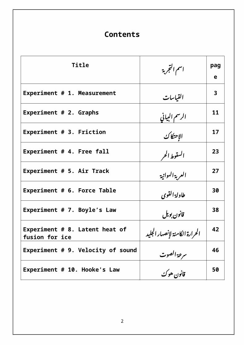
The Vernier Caliper is a precision instrument that can be used to measure internal and external distances extremely accurately. The example shown below is a manual caliper. Measurements are interpreted from the scale by the user. This is more difficult than using a digital Vernier caliper which has an LCD digital display on which the reading appears. The manual version has both an imperial and metric scale.Manually operated Vernier calipers can still be bought and remain popular because they are much cheaper than the digital version. Also, the digital version requires a small battery whereas the manual version does not need any power source.

HOW TO READ A MEASUREMENT FROM THE SCALES

Example 1: The external measurement (diameter) of a round section piece of steel is measured using a Vernier caliper, metric scale.

3

Mathematical Method

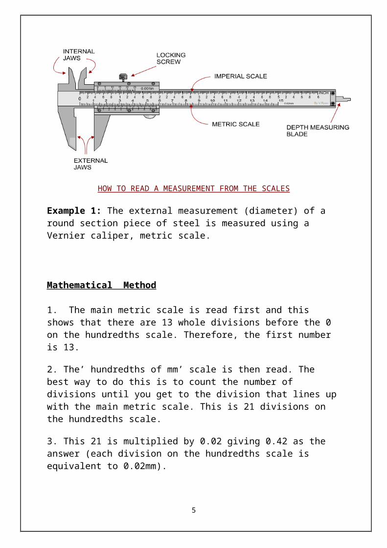
1. The main metric scale is read first and this shows that there are 13 whole divisions before the 0 on the hundredths scale. Therefore, the first number is 13.

2. The’ hundredths of mm’ scale is then read. The best way to do this is to count the number of divisions until you get to the division that lines up with the main metric scale. This is 21 divisions on the hundredths scale.

3. This 21 is multiplied by 0.02 giving 0.42 as the answer (each division on the hundredths scale is equivalent to 0.02mm).

4. The13 and the 0.42 are added together to give the final measurement of 13.42mm (the diameter of the piece of round section steel)

Commonness Method

alternatively, it is just as easy to read the 13 on the main scale and 42 on the hundredths scale. The correct measurement being 13.42mm.

Example 2 : (To zoom in to see the scale - right click mouse and select zoom)

4

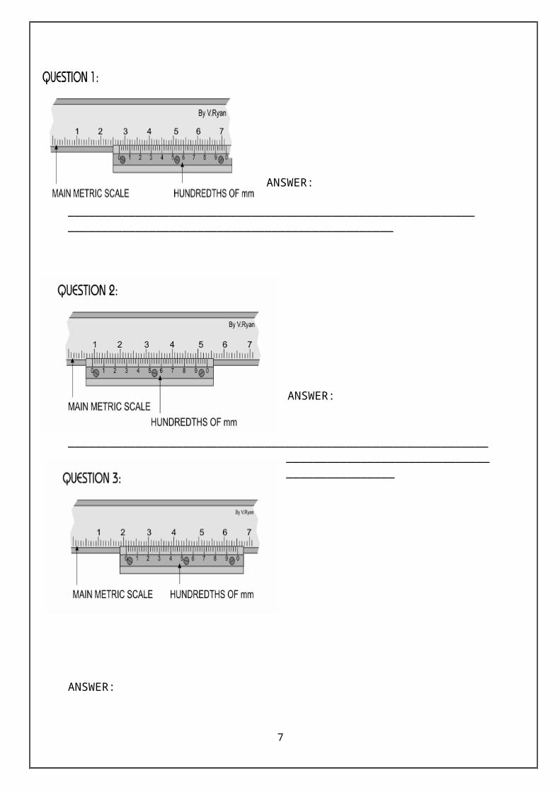
ANSWER:____________________________________________________________________________________________________________

5

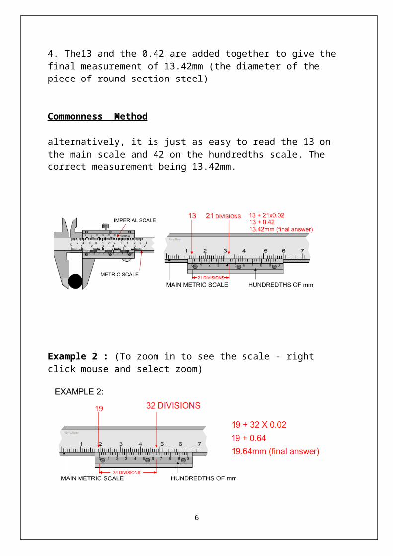
ANSWER:____________________________________________________________________________________________________________

ANSWER:

____________________________________________________________________________________________________________

6

The Micrometer

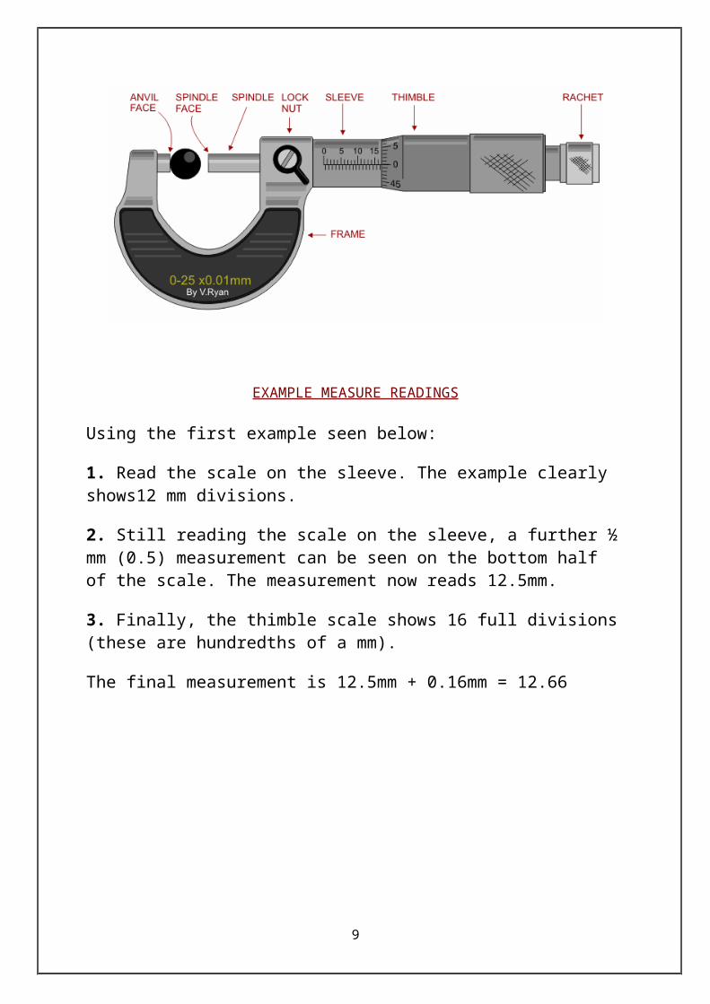
The micrometre is a precision measuring instrument, used by engineers. Each revolution of the rachet moves the spindle face 0.5mm towards the anvil face. The object to be measured is placed between the anvil face and the spindle face. The rachet is turned clockwise until the object is ‘trapped’ between these two surfaces and the rachet makes a ‘clicking’ noise. This means that the rachet cannot be tightened anymore and the measurement can be read.

EXAMPLE MEASURE READINGS

Using the first example seen below:

1. Read the scale on the sleeve. The example clearly shows12 mm divisions.

2. Still reading the scale on the sleeve, a further ½ mm (0.5) measurement can be seen on the bottom half of the scale. The measurement now reads 12.5mm.

3. Finally, the thimble scale shows 16 full divisions (these are hundredths of a mm).

The final measurement is 12.5mm + 0.16mm = 12.66

7

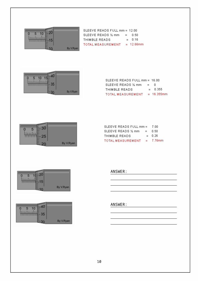
ANSWER:

ANSWER:

8

ANSWER:

Experiment #1

9

Measurements

Name:…………… … Registration number:……… …….

Date:…………………… Mark:………………………….

Results and Discussions

1- The aim ……………………………………………………………………………………..............…………………………………………………………………………..…………………………………………………………………………………… ..............…………………………………………………………………………..

1) By using the Vernier caliper :*calculate the size of the cuboid………………………………………………………………………………………………………………………………………………………………………………………………………………………………………………………………

* calculate the radius of the tube………………………………………………………………………………………………………………………………………………………………………………………………………………………………………………………………

2) By using the micrometer :

*calculate the size of the ball………………………………………………………………………………………………………………………………………………………………………………………………………………………………………………………………

* calculate the radius of the wire………………………………………………………………………………………………………………………………………………………………………………………………………………………………………………………………Experiment #2 Graphs

10

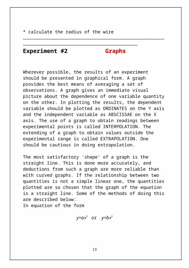
Wherever possible, the results of an experiment should be presented in graphical form. A graph provides the best means of averaging a set of observations. A graph gives an immediate visual picture about the dependence of one variable quantity on the other. In plotting the results, the dependent variable should be plotted as ORDINATES on the Y axis and the independent variable as ABSCISSAE on the X axis. The use of a graph to obtain readings between experimental points is called INTERPOLATION. The extending of a graph to obtain values outside the experimental range is called EXTRAPOLATION. One should be cautious in doing extrapolation.

The most satisfactory 'shape' of a graph is the straight line. This is done more accurately, and deductions from such a graph are more reliable than with curved graphs. If the relationship between two quantities is not a simple linear one, the quantities plotted are so chosen that the graph of the equation is a straight line. Some of the methods of doing this are described below: In equation of the form

y=ax2 or y=bx3

If y is plotted against x, curves are obtained. The resulting graph may be a straight line if y is plotted against x2 or x3.

The time-period of a simple pendulum is given by T=2π √l / g .

If T is plotted against 1, a quadratic curve is obtained. The equation can be converted to the form T 2=4 π2 . l

g to give a straight line between l and T 2. The curve, between the pressure p and the volume V of a given mass of gas at constant temperature, is an inverse curve as the relation between them is expressed as

pV = k, where k is a constant.

The equation can be written in the form p=k . 1

V

The graph of p, when plotted against 1/V, is a straight line.

Steps in Plotting a Graph:-

11

1. Plotting the variables:When a student is told to plot, say, S versus t, it is important that he understands the following:

a. t is the independent variable, which is the quantity that is deliberately varied or changed. The independent variable is plotted on the "x" or horizontal axis.

b. S is the dependent variable, which is the quantity that changes due to the variation in the independent variable. The dependent variable is plotted on the "y" or vertical axis. This is a convention (agreement) which should be memorized.

2. Labeling the axes:

The vertical and horizontal axes of the graph paper should carry labels indicating the quantities plotted, with units. In our previous example the label on the y-axis would be: S (m).

3. Choosing the scale:The scale for a variable is the number of centimeters of length of the graph paper given to a unit of the variable being plotted. For example, one might allow 1 cm for each 10 seconds of time. Note that in general the scales along the x and y axes may be different.

Two things need careful consideration before choosing the scales for a graph, the ranges of the variables, and convenience in plotting:

a) Range of the variable

12

Suppose a student has some data for a variable S which ranges from 5*10-2 m to 125*10-2 m. He then should choose a scale which allows him to plot S values from zero to values somewhat greater than 125*10-2 m.

Notice in this case that, unless told to do so by the instructor, he does not choose to suppress the zero and start the S scale from 5*10-2 m. The reason is that later he may need to use the graph to find values extrapolated (continued) to the origin. Also, he allows space on the graph for values somewhat greater than the largest value in the data set (in our example, 125*10-2 m). He does this because later some more data, with larger values, may be acquired, or he might need to extrapolate the graph to larger values.

Finally, the scale should be chosen to most nearly use the whole of the graph paper. Just because a simple choice (say, 1 cm to 1 second of time) makes a graph easy to plot, this should not be done if it results in a tiny graph "hiding" in a corner of the sheet of paper! Besides not looking "nice", such a graph is also inaccurate when used to analyze the data.

b) Convenience in plottingIt turns out that scales of 1, 2, 5 and 10 (and multiples of 10 of these) per centimeter are easiest to use; a scale of 4 per centimeter is somewhat more difficult but can be used. Scales of 3, 6, 7, 9, etc. per centimeter are very difficult to plot and read and In choosing scales it sometimes helps to turn the paper so that the "x-axis" is either the long or short dimension of the paper.

13

Unsuitable scale for x- axes Suitable scale for bothaxes

4. Circling the data Points:

When plotting graphs by hand use a pencil. Pencil marks are easier to erase if you make a mistake! Use a dot enclosed in a circle, or a cross.

5. Drawing a Straight Line through the Data Points:

When the data fall on a straight line (or are expected theoretically to do so) a ruler may be used to draw a straight line through the points. Observe the following rules: the line is drawn to match the data trend, and for data with some "scatter" balance some points above and below the line. In general, the best straight line is the line that, on average, is closest to all of the points. Finally, points which fall far outside the general data trend should be double-checked for correct plotting, then, if found correctly plotted, ignored in drawing the line.

Graphical Analysis :

Calculating the slope:For data sets (x, y) obeying a linear relation y = mx + b, we can use a graph of the data to determine the values of m and b. On the graph these are found to be:

b: y-intercept of the graph (value of y when x = 0.)(b= V.I=5*100 N/m2)

14

Unsuitable scale for both axes Unsuitable scale for y- axes

m: slope of the graph = ∆ y∆ x

=y2− y1

x2−x1

m = (7−5 )∗10010−0

=20 N /m2∗C

Note that in finding the slope we should choose the points (x1 , y1), (x2 , y2 ) relatively far apart for accuracy. These values should not be chosen to correspond to data points even if they appear to lie on the straight line.

Experiment #2

Graphs

15


Date:…………………… Mark:………………………….

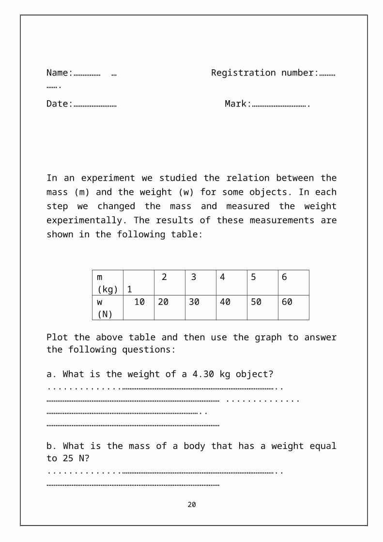
In an experiment we studied the relation between the mass (m) and the weight (w) for some objects. In each step we changed the mass and measured the weight experimentally. The results of these measurements are shown in the following table:

m (kg)

1 2 3 4 5 6

w (N) 10 20 30 40 50 60 Plot the above table and then use the graph to answer the following questions:

a. What is the weight of a 4.30 kg object? ..............…………………………………………………………………………..…………………………………………………………………………………… ..............…………………………………………………………………………..…………………………………………………………………………………… b. What is the mass of a body that has a weight equal to 25 N? ..............…………………………………………………………………………..…………………………………………………………………………………… ..............…………………………………………………………………………..……………………………………………………………………………………

c. Is the above table enough to find accurate answers for parts a and b..............…………………………………………………………………………..…………………………………………………………………………………… ..............…………………………………………………………………………..…………………………………………………………………………………… Experiment #3 Friction

16

The aim of experiment:

1. Studying the friction between two rough surfaces.

2. Determination of the coefficient of static friction (µs).

3. Determination of the coefficient of kinetic friction (µk).

Theory of experiment:

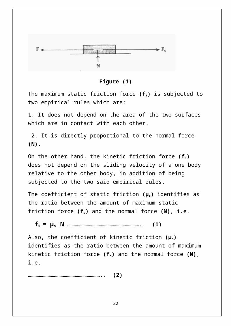
Friction is the resistance of motion which originates between two surfaces which are in contact with each other. The friction force (f) between two static objects called the static friction force (fs), while it called the kinetic friction force (fk) in case of being between two moving surfaces. Look at figure (1).

Figure (1)

The maximum static friction force (fs) is subjected to two empirical rules which are:

1. It does not depend on the area of the two surfaces which are in contact with each other.

2. It is directly proportional to the normal force (N).

On the other hand, the kinetic friction force (fk) does not depend on the sliding velocity of a one body relative to the other body, in addition of being subjected to the two said empirical rules.

The coefficient of static friction (µs) identifies as the ratio between the amount of maximum static friction force (fs) and the normal force (N), i.e.

fs = µs N ………………………………………………………….. (1)

Also, the coefficient of kinetic friction (µk) identifies as the ratio between the amount of maximum kinetic friction force (fk) and the normal force (N), i.e.

17

………………………………………………………….. (2)

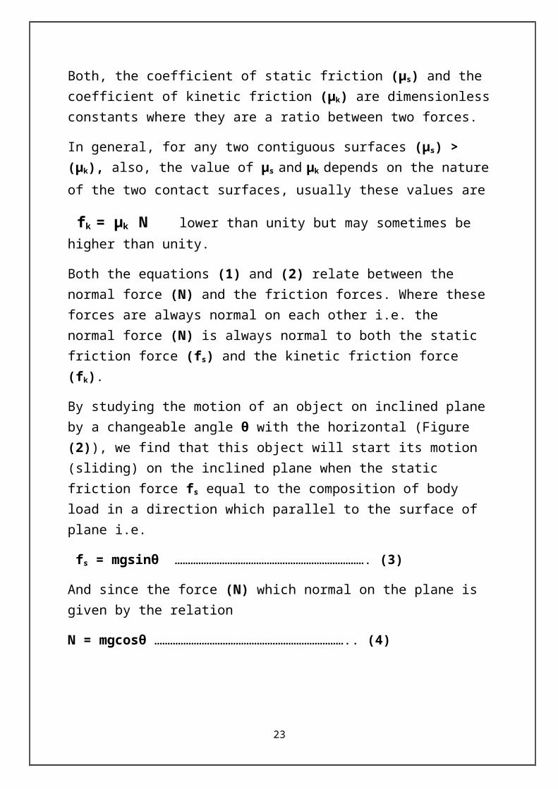
Both, the coefficient of static friction (µs) and the coefficient of kinetic friction (µk) are dimensionless constants where they are a ratio between two forces.

In general, for any two contiguous surfaces (µs) > (µk), also, the value of µs and

µk depends on the nature of the two contact surfaces, usually these values are

fk = µk N lower than unity but may sometimes be higher than unity.

Both the equations (1) and (2) relate between the normal force (N) and the friction forces. Where these forces are always normal on each other i.e. the normal force (N) is always normal to both the static friction force (fs) and the kinetic friction force (fk).

By studying the motion of an object on inclined plane by a changeable angle θ with the horizontal (Figure (2)), we find that this object will start its motion (sliding) on the inclined plane when the static friction force fs equal to the composition of body load in a direction which parallel to the surface of plane i.e.

fs = mgsinθ ………………………………………………………………. (3)

And since the force (N) which normal on the plane is given by the relation

N = mgcosθ ……………………………………………………………….. (4)

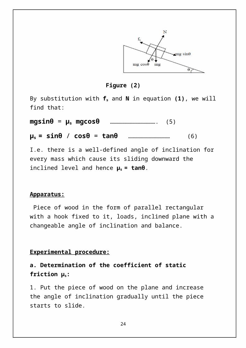
Figure (2)

By substitution with fs and N in equation (1), we will find that:

mgsinθ = µs mgcosθ …………………………………. (5)

µs = sinθ / cosθ = tanθ ……………………………… (6)

18

I.e. there is a well-defined angle of inclination for every mass which cause its sliding downward the inclined level and hence µs = tanθ.

Apparatus:

Piece of wood in the form of parallel rectangular with a hook fixed to it, loads, inclined plane with a changeable angle of inclination and balance.

Experimental procedure:

a. Determination of the coefficient of static friction µs:

1. Put the piece of wood on the plane and increase the angle of inclination gradually until the piece starts to slide.

2. Fix the inclination angle of plane at the angle where inclination began then read the angle and record it.

3. Calculate the coefficient of static friction µs from the equation:

µs = tanθ

b. Determination of the coefficient of kinetic friction µk:

1. Clean the plane and the wood piece then weight the wood piece.

2. Find the normal force N of the wood piece and record it in the table.

(N = mg).

3. Fix the balance to the hook of the wood piece and pull it until moving of the wood piece and record the reading in the table of results, the applied force F.

4. Put a load of 20 gm on the wood piece, Pull it and record the applied force F in the table with recording of the normal force N.

5. Repeat step (4) for loads of 40, 60, 80 … etc. with recording of the results.

6. Plot the relation between the applied force (F) and the normal force (N).

7. Find the slop of the straight line, where slope = F/N

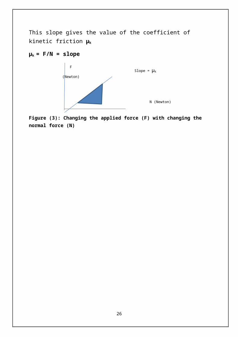
This slope gives the value of the coefficient of kinetic friction µk

19

µk = F/N = slope

Figure (3): Changing the applied force (F) with changing the normal force (N)

Experiment #3

Friction

20

F

(Newton)

N (Newton)

Slope = µk


Date:…………………… Mark:………………………….

1- The aim ……………………………………………………………………………………..............…………………………………………………………………………..…………………………………………………………………………………… ..............…………………………………………………………………………..(2) Complete the missing parts in the following:

1. Friction is the resistance of motion which originates between ………….

2. Friction force between ……………… is called the static friction force (f s), while it called the kinetic friction force (fk) in case of being between ………

3. The static friction force is …………….Proportional to the normal force which acts on the surface of contact.

4. The coefficient of static friction (µs) identifies by the relation ……………, while the coefficient of kinetic friction (µk) identifies by the relation ……….

5. For any two surfaces which are in contact with each other (µs).………. (µk).

Results

a- Determination of the coefficient of static friction (µs)

……………………………………………………………………………………..............…………………….……………………………………………………..………………………………………………………………

b- Determination of the coefficient of kinetic friction (µk)

Number

Mass of wood piece and its overload

m (kg)

The normal force

N = mg

The applied force

F

µk = F/ mg

21

(Newton) (Newton)1

2

3

4

5

……………………………………………………………………………………..............…………………………………………………………………………..…………………………………………………………………………………… ..............………………………………………………………………………….. ……………………………………………………………………………………

c- Draw the relation between F and N, determine the (µk).

Experiment # 4 Free fall


22

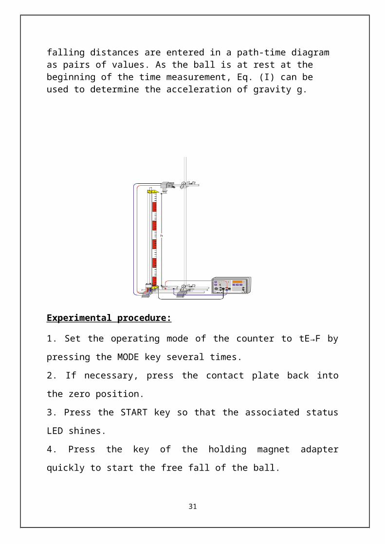
1. Measuring the falling times of a ball between the holding magnet and the contact plate for recording the path-time diagram point by point.

2. Confirming the proportionality between the falling distance and the square of the falling time.

3. Determining the acceleration of gravity.


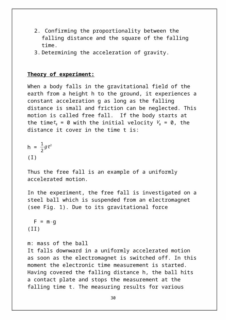
When a body falls in the gravitational field of the earth from a height h to the ground, it experiences a constant acceleration g as long as the falling distance is small and friction can be neglected. This motion is called free fall. If the body starts at the timet 0 = 0 with the initial velocity V 0 = 0, the distance it cover in the time t is:

h = 12

g t2 (I)

Thus the free fall is an example of a uniformly accelerated motion. In the experiment, the free fall is investigated on a steel ball which is suspended from an electromagnet (see Fig. 1). Due to its gravitational force

F = m⋅g (II)

m: mass of the ball It falls downward in a uniformly accelerated motion as soon as the electromagnet is switched off. In this moment the electronic time measurement is started. Having covered the falling distance h, the ball hits a contact plate and stops the measurement at the falling time t. The measuring results for various falling distances are entered in a path-time diagram as pairs of values. As the ball is at rest at the beginning of the time measurement, Eq. (I) can be used to determine the acceleration of gravity g.

23

Experimental procedure:

1. Set the operating mode of the counter to tE→F by pressing the MODE key

several times.

2. If necessary, press the contact plate back into the zero position.

3. Press the START key so that the associated status LED shines.

4. Press the key of the holding magnet adapter quickly to start the free fall of the

ball.

5.When the ball has hit the contact plate, read the falling time and take it down.

6.Reduce the falling distance h by 5 cm by lowering the holding magnet, press

the contact plate into its zero position, and reset the counter S to zero by

pressing the Start key.

7. Suspend the ball anew, and repeat the measurement.

8.Reduce the falling distance in steps of 5 cm, each time repeating the

measurement.

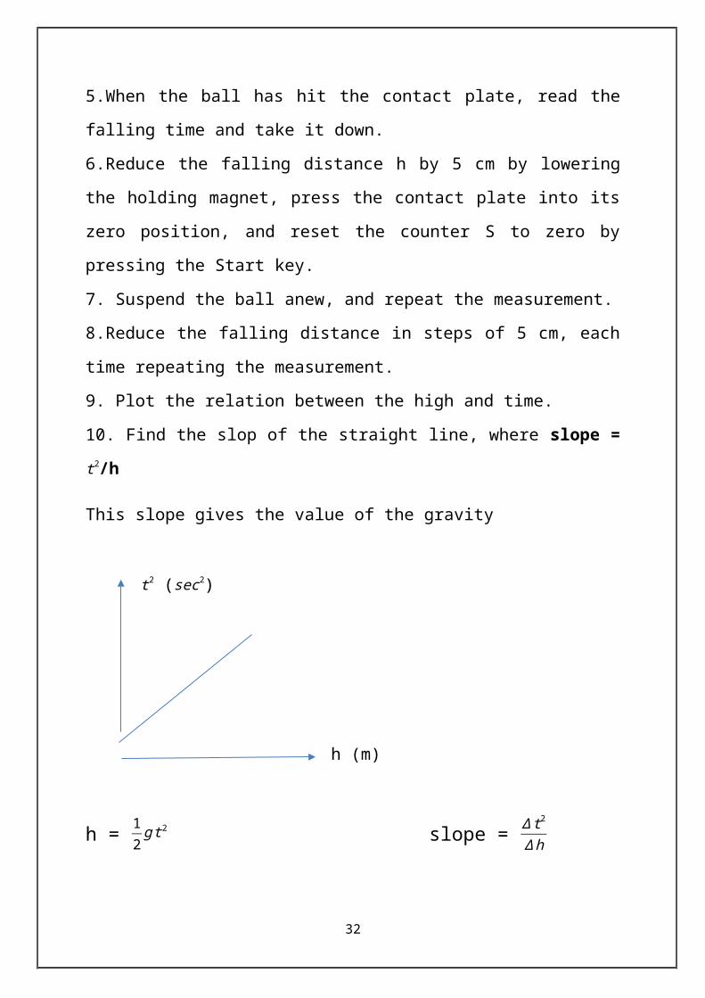
9. Plot the relation between the high and time.

10. Find the slop of the straight line, where slope = t 2/h

This slope gives the value of the gravity

24

h = 12

g t2 slope = ∆ t 2

∆ h

g = 2ht 2 g = 2

slope

25

h (m)

t 2 (sec2)

Experiment # 4 Free fall


Date:…………………… Mark:………………………….

1- The aim ……………………………………………………………………………………..............…………………………………………………………………………..…………………………………………………………………………………… ..............…………………………………………………………………………..


Tabulate the results in the following table:

∆ h t 1 t 2 t 3 t t 2

……………………………………………………………………………………..............…………………………………………………………………………..…………………………………………………………………………………… ..............………………………………………………………………………….. ……………………………………………………………………………………..............…………………………………………………………………………..…………………………………………………………………………………… ..............…………………………………………………………………………..

26

Experiment # 5 Air Track


The purpose of this lab experiment is to study the motion in one dimension of a glider on an air track.


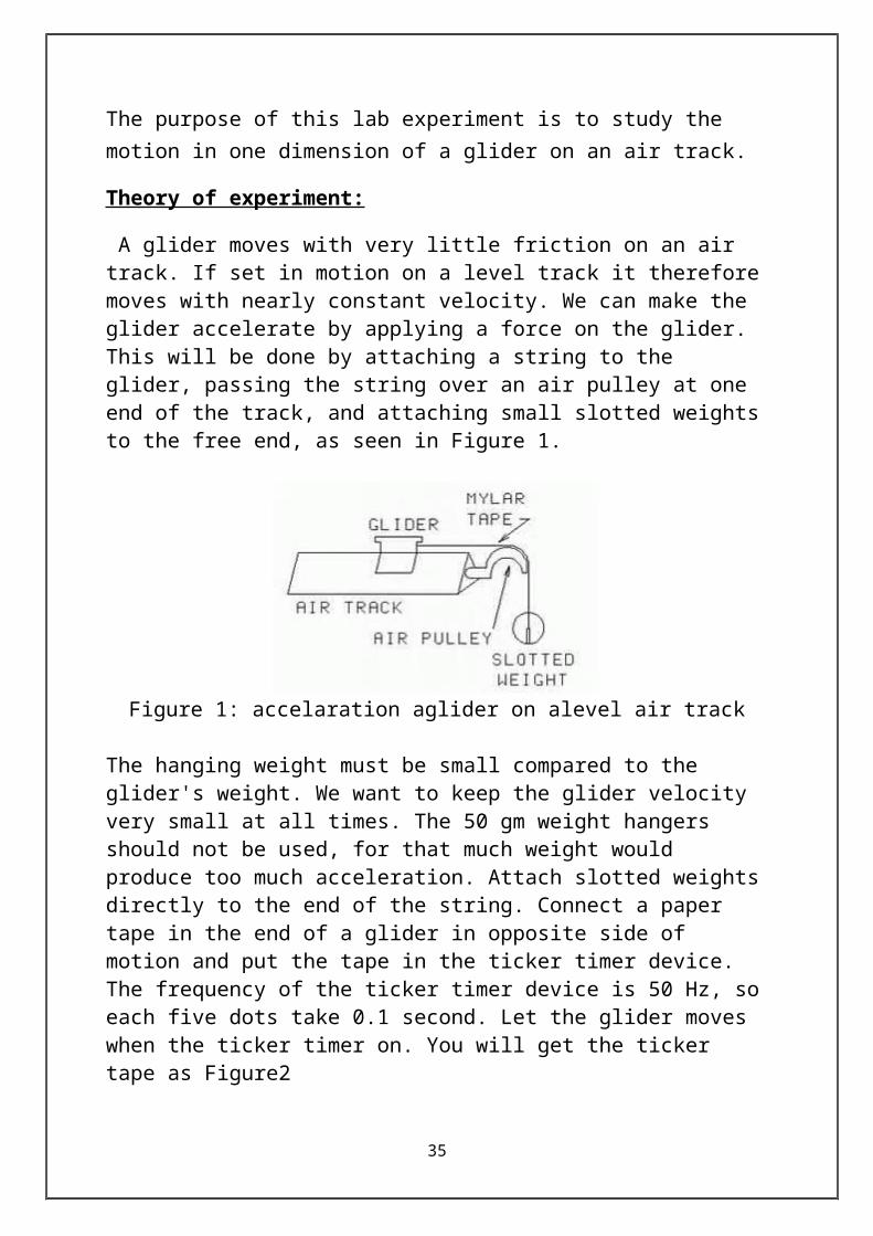
A glider moves with very little friction on an air track. If set in motion on a level track it therefore moves with nearly constant velocity. We can make the glider accelerate by applying a force on the glider. This will be done by attaching a string to the glider, passing the string over an air pulley at one end of the track, and attaching small slotted weights to the free end, as seen in Figure 1.

Figure 1: accelaration aglider on alevel air track

The hanging weight must be small compared to the glider's weight. We want to keep the glider velocity very small at all times. The 50 gm weight hangers should not be used, for that much weight would produce too much acceleration. Attach slotted weights directly to the end of the string. Connect a paper tape in the end of a glider in opposite side of motion and put the tape in the ticker timer device. The frequency of the ticker timer device is 50 Hz, so each five dots take 0.1 second. Let the glider moves when the ticker timer on. You will get the ticker tape as Figure2

27

Figure.2 : A scheme of ticker timer tape.

Use the equation of motion in one dimension. ∆x = xf - xi

vavg=∆ x∆ t

=x f−xi

t f −¿ti3.1¿

v=dxdt

aavg=∆ v∆t

3.2

a=dvdt

Where ∆x is the displacement, vavg and v are the average and instantaneous velocity, respectively. aavg and a is average and instantaneous acceleration, respectively.

Apparatus:

Air track, air pump, a glider, hunger mass, metric ruler, pulley, string, ticker timer device, and ticker timer tape.

Experimental Procedure:

1. Set a glider and all devices as Figure 1.

2. Switch on the air pump and ticker timer device.

3. Let a glider to accelerate.

4. Analyzing the ticker timer tape.

5. Find the average velocity and acceleration.

28

…. . . . . . . . . . . . . . . . . . .

Experiment # 5

Air Track


Date:…………………… Mark:………………………….

1- The aim

.................................................................................................................

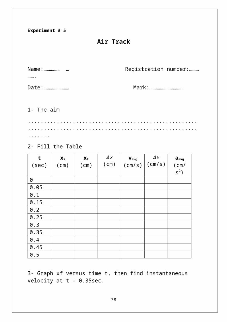
2- Fill the Table

t(sec)

xi

(cm)xf

(cm)∆ x

(cm)vavg

(cm/s)∆ v

(cm/s)aavg

(cm/s2)00.050.10.150.20.250.30.350.40.450.5

3- Graph xf versus time t, then find instantaneous velocity at t = 0.35sec. ………………………………………………………………………………………… …………………………………………………………………………………………

4- Graph vavg versus time t, and then find the slope? ………………………………………………………………………………………… …………………………………………………………………………………………

5- Find the acceleration a from Q4?

………………………………………………………………………………………… ………………………………………………………………………

29

Experiment # 6 Force Table


1. To provide a laboratory experience in the addition of vectors2. To investigate whether forces follow the vector law of addition


Some physical quantities have only magnitude as, for example, volume and density.These quantities are called scalars. The student is familiar with addition, subtraction, multiplication and division of scalars. Other physical quantities such as velocity, acceleration and force need to have a direction as well as a magnitude specified. These quantities are called vectors. The algebra of vectors is more sophisticated than the algebra of scalars.We will study in this experiment only concurrent vectors (vectors which pass through one point). The vector physical quantities, which we study here, are forces.

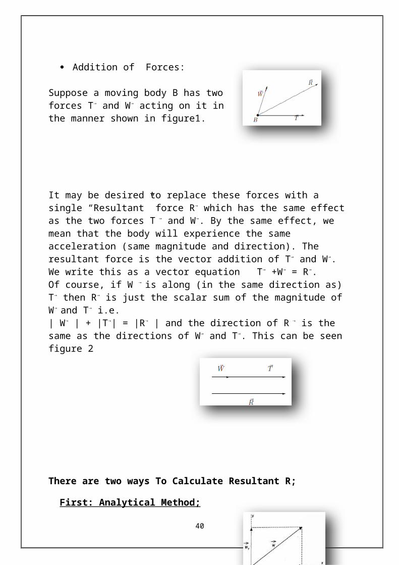
Addition of Forces:

Suppose a moving body B has two forces T→

and W→ acting on it in the manner shown in figure1.

It may be desired to replace these forces with a single “Resultant” force R→ which has the same effect as the two forces T → and W→. By the same effect, we mean that the body will experience the same acceleration (same magnitude and direction). The resultant force is the vector addition of T→ and W→. We write this as a vector equation T→ +W→ = R→. Of course, if W → is along (in the same direction as) T→ then R→ is just the scalar sum of the magnitude of W→ and T→ i.e.| W→ | + |T→| = |R→ | and the direction of R → is the same as the directions of W→

and T→. This can be seen figure 2

30

There are two ways To Calculate Resultant R;

First: Analytical Method;

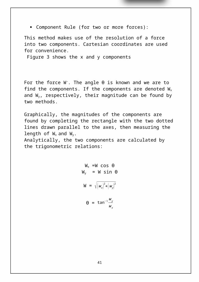
Component Rule (for two or more forces):

This method makes use of the resolution of a force into two components. Cartesian coordinates are used for convenience. Figure 3 shows the x and y components

For the force W→. The angle Ө is known and we are to find the components. If the components are denoted Wx and Wy, respectively, their magnitude can be found by two methods.

Graphically, the magnitudes of the components are found by completing the rectangle with the two dotted lines drawn parallel to the axes, then measuring the length of Wx and Wy.Analytically, the two components are calculated by the trigonometric relations:

Wx =W cos ӨWy = W sin Ө

W = √ (w x )2+(w y )2

Ө = tan−1 w y

w x

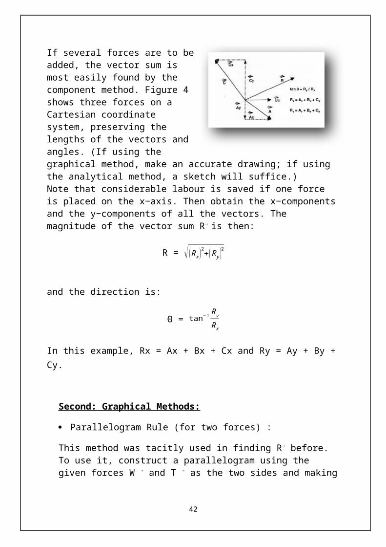
If several forces are to be added, the vector sum is most easily found by the component method. Figure 4 shows three forces on a Cartesian coordinate

31

system, preserving the lengths of the vectors and angles. (If using the graphical method, make an accurate drawing; if using the analytical method, a sketch will suffice.)Note that considerable labour is saved if one force is placed on the x−axis. Then obtain the x−components and the y−components of all the vectors. The magnitude of the vector sum R→ is then:

R = √ ( Rx)2+( R y )2

and the direction is:

Ө = tan−1 Ry

Rx

In this example, Rx = Ax + Bx + Cx and Ry = Ay + By + Cy.

Second: Graphical Methods:

Parallelogram Rule (for two forces) :

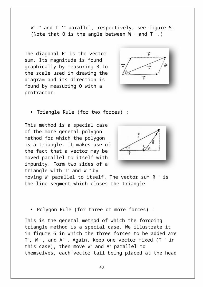
This method was tacitly used in finding R→ before. To use it, construct a parallelogram using the given forces W → and T → as the two sides and making W '→ and T '→ parallel, respectively, see figure 5. (Note that Ө is the angle between W → and T →.)

The diagonal R→ is the vector sum. Its magnitude is found graphically by measuring R to the scale used in drawing the diagram and its direction is found by measuring Ө with a protractor.

Triangle Rule (for two forces) :

This method is a special case of the more general polygon method for which the polygon is a triangle. It makes use of the fact that a vector may be moved

32

parallel to itself with impunity. Form two sides of a triangle with T→ and W → by moving W→ parallel to itself. The vector sum R → is the line segment which closes the triangle

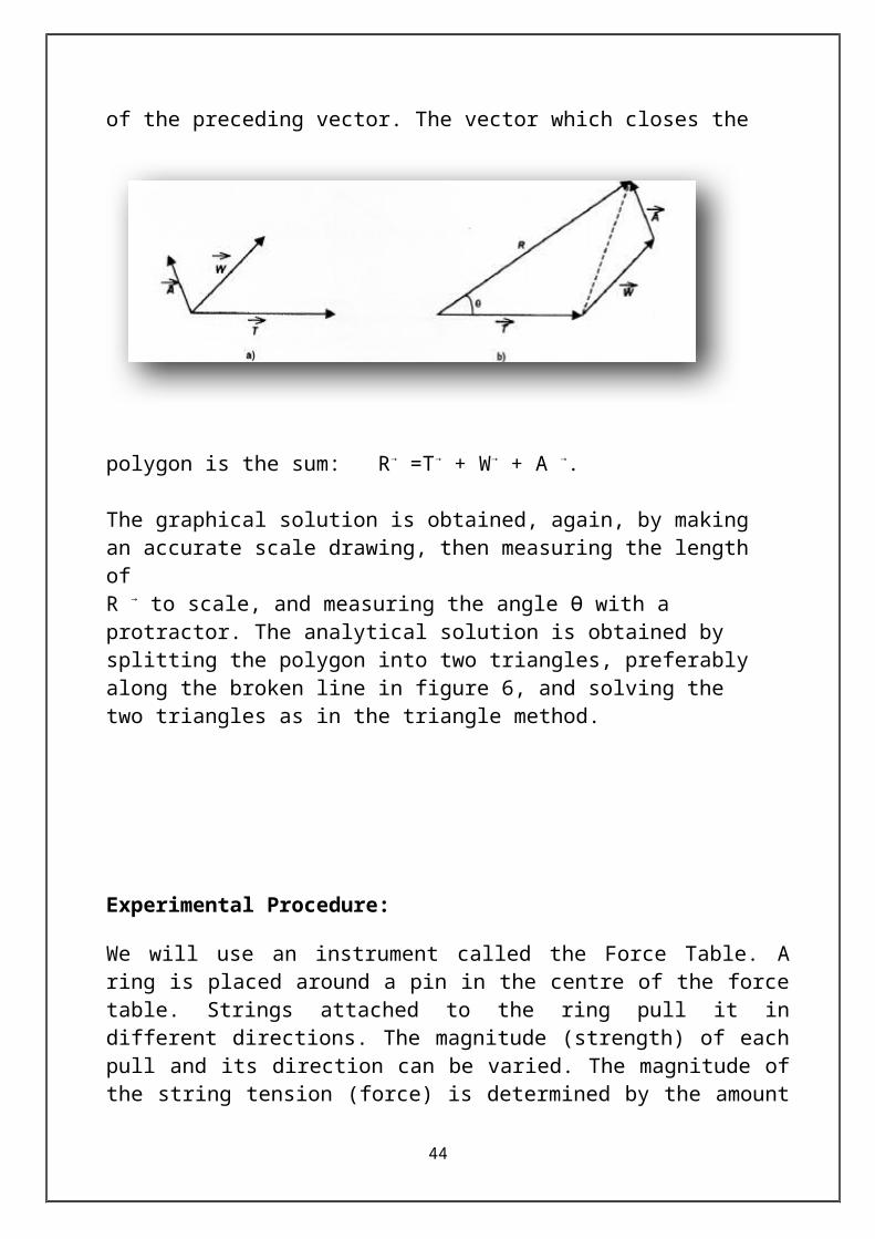
Polygon Rule (for three or more forces) :

This is the general method of which the forgoing triangle method is a special case. We illustrate it in figure 6 in which the three forces to be added are T→, W→ , and A→ . Again, keep one vector fixed (T → in this case), then move W→ and A→ parallel to themselves, each vector tail being placed at the head of the preceding vector. The vector which closes the polygon is the sum: R→ =T→ +

W→ + A →.

The graphical solution is obtained, again, by making an accurate scale drawing, then measuring the length of R → to scale, and measuring the angle Ө with a protractor. The analytical solution is obtained by splitting the polygon into two triangles, preferably along the broken line in figure 6, and solving the two triangles as in the triangle method.


33

We will use an instrument called the Force Table. A ring is placed around a pin in the centre of the force table. Strings attached to the ring pull it in different directions. The magnitude (strength) of each pull and its direction can be varied. The magnitude of the string tension (force) is determined by the amount of mass which is hung from the other end of the string. The value of the pull (force) is mg, where g = 9.81 m/s2. The force table allows you to demonstrate when the sum of forces acting on the ring equals zero. Under this equilibrium condition, the ring, when released will remain on the spot.

Mount the Force Table in parallel to the working desk (horizontal position). Be sure that it is level.

Experiment with two forces:

1. Place a pulley at the 30o mark on the Force Table and place a total of 0.35 kg (which includes 0.05 kg of the mass holder) on the end of the string. Place a second pulley at 130o mark and place a total of 0.25 kg (including 0.05 kg of the mass holder). Calculate the magnitude of the forces produced by these masses and record them in Table 1.

2. Determine by trial and error the magnitude of mass needed and the angle at which it must be placed in order to place the ring in equilibrium. The ring is in equilibrium when it is centred on the Force Table. Be sure that all the strings are in such a position that they are directed along a line that passes through the centre of the ring.

3. From the experimentally determined mass, calculate the force produced and record the magnitude and direction of this equilibrant force in Table 1.

4. From the value of the equilibrant force, determine the magnitude and direction of the resultant force and record them in Table 1

Calculations:

1. Find the resultant of these two applied forces by scaled graphical construction using the Triangle method. Using a ruler and a protractor, construct vectors whose scaled length and direction represent F1 and F2. A convenient scale might be 1 graphical division = 0.1 N. Read the magnitude and direction of the resultant from your graphical solution and record them in Table 2.

2. Using equation 1, calculate the components of F1 and F2 and record them into the analytical solution portion of Table 2. Add the components algebraically and determine the magnitude of the resultant by the Pythagorean theorem. Determine the angle of the resultant.

3. Calculate the percentage error of the magnitude of the experimental value of FR compared to the analytical solution of FR. Also calculate the percentage

34

error of the magnitude of the graphical solution of FR compared to the analytical solution.

Results:

TABLE 1

Experimental (Force Table)

Force Mass(Kg) Force(N) Direction (Ө)

F1 0.25 30°

F2 0.35 130°

Equilibrant FE

Resultant FR

35

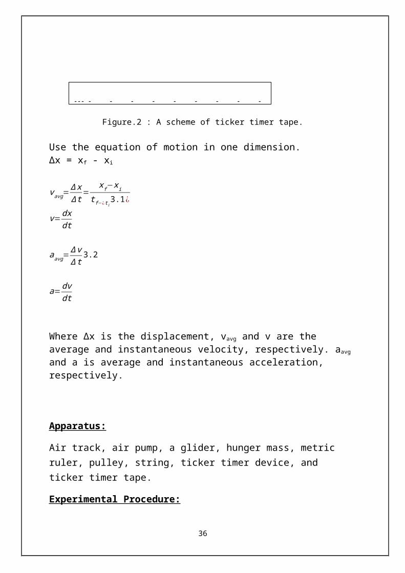
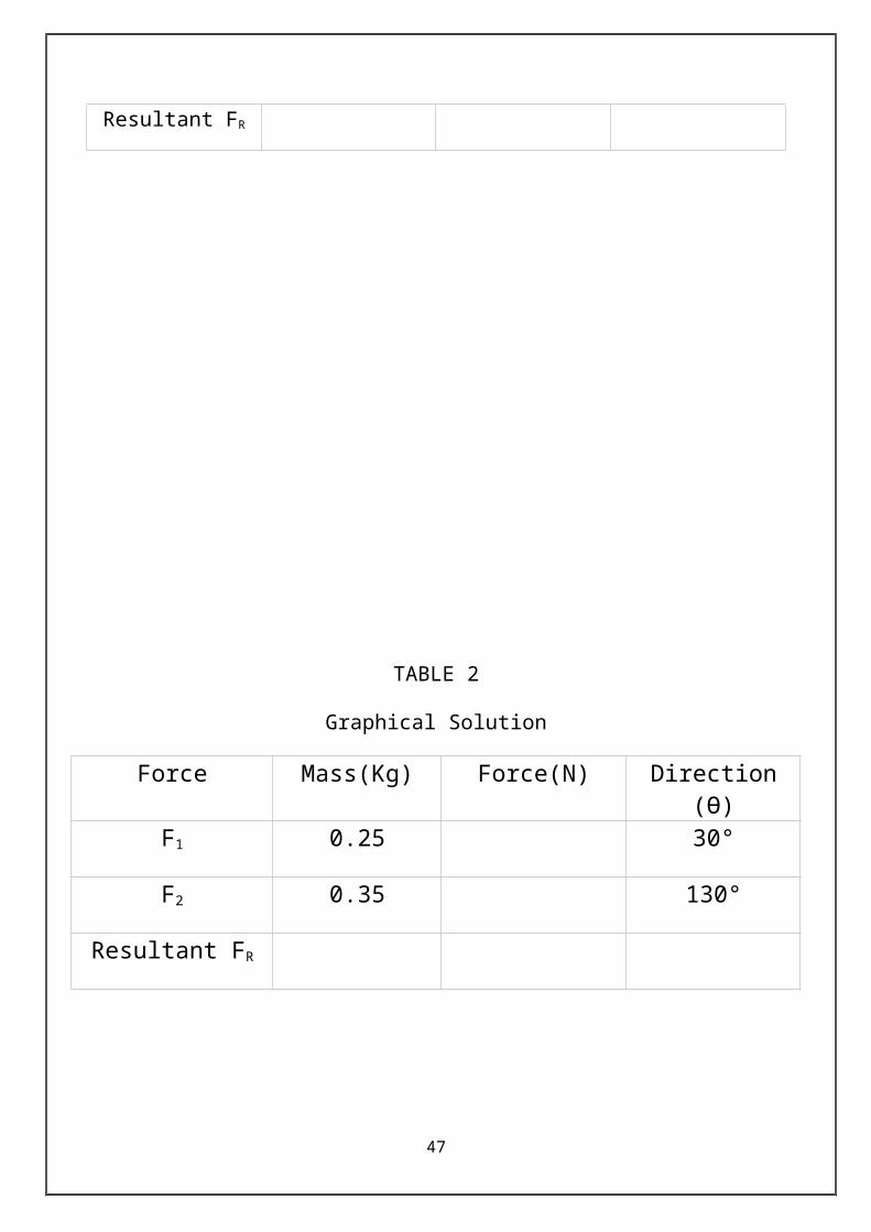
TABLE 2

Graphical Solution


F1 0.25 30°

F2 0.35 130°

Resultant FR

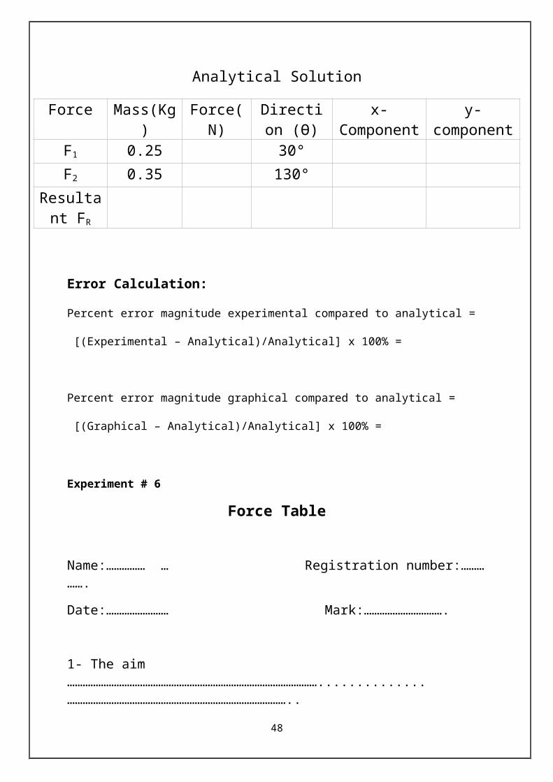
Analytical Solution


x-Component y-component

F1 0.25 30°F2 0.35 130°

Resultant FR

Error Calculation:

Percent error magnitude experimental compared to analytical =

[(Experimental – Analytical)/Analytical] x 100% =

Percent error magnitude graphical compared to analytical =

[(Graphical – Analytical)/Analytical] x 100% =

36

Experiment # 6

Force Table


Date:…………………… Mark:………………………….

1- The aim ……………………………………………………………………………………..............…………………………………………………………………………..…………………………………………………………………………………… ..............…………………………………………………………………………..


2- What is the magnitude and direction of the equilibrant force that you found by force table?…………………………………………………………………………………… ..............…………………………………………………………………………..

3- What is the magnitude and direction of the resultant force that you found by force table?

…………………………………………………………………………………… ..............…………………………………………………………………………..

4- Find the magnitude and direction of the resultant force by using graphical method?

…………………………………………………………………………………… ..............…………………………………………………………………………..

5- Find the magnitude and direction of the resultant force by using component method?

…………………………………………………………………………………… ..............…………………………………………………………………………..

37

Experiment # 7 BOYLE’S LAW


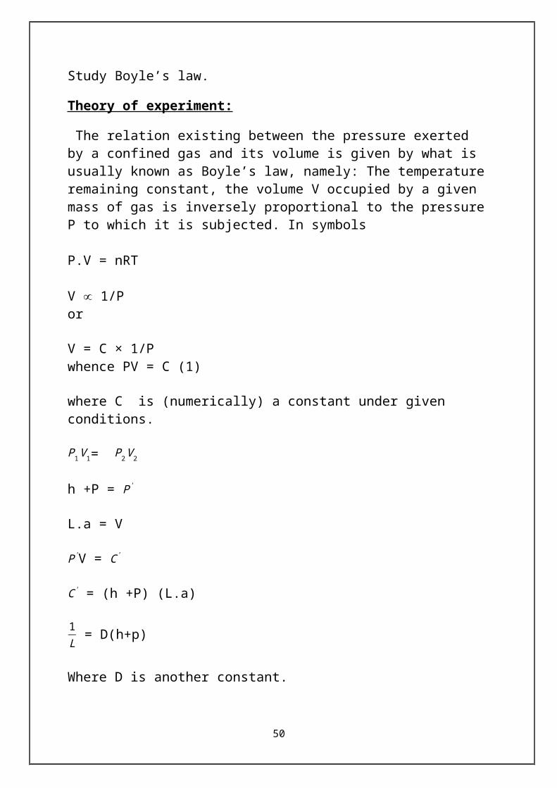
Study Boyle’s law.


The relation existing between the pressure exerted by a confined gas and its volume is given by what is usually known as Boyle’s law, namely: The temperature remaining constant, the volume V occupied by a given mass of gas is inversely proportional to the pressure P to which it is subjected. In symbols

P.V = nRT

V ∝ 1/Por

V = C × 1/Pwhence PV = C (1)

where C is (numerically) a constant under given conditions.

P1V 1= P2V 2

h +P = P'

L.a = V

P'V = C '

C ' = (h +P) (L.a)

1L = D(h+p)

Where D is another constant.

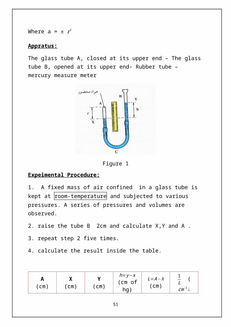
Where a = r2

38

Appratus:

The glass tube A, closed at its upper end – The glass tube B, opened at its upper end- Rubber tube – mercury measure meter

Figure 1

Expeimental Procedure:

1. A fixed mass of air confined in a glass tube is kept at room-temperature and subjected to various pressures. A series of pressures and volumes are observed.

2. raise the tube B 2cm and calculate X,Y and A .

3. repeat step 2 five times.

4. calculate the result inside the table.

1L (cm−1 ¿

L=A−X(cm)

h= y−x(cm of hg)

Y(cm)

X(cm)

A(cm)

39

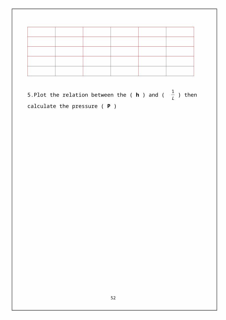
5.Plot the relation between the ( h ) and ( 1L ) then calculate the pressure ( P )

40

Experiment # 7BOYLE’S LAW


Date:…………………… Mark:………………………….

Choose the correct answer:

1) which law explains an inverse relationship between the fixed mass of ideal gas at fixed temperature and pressure of a gas:a) Charles' lawb) Dalton's lawc) Boyle's law

2) the relationship between the (V) and (P):a) Inverseb) Direct

3) the relationship between the (V) and (P) in the Boyle's law is in the form of:a) A straight lineb) A curve

4) In Boyle's law:a) pv≠ c

b) pv=c

c) pv=c2

41

Experiment # 8 HEAT OF FUSION


Determining the Specific Heat of Fusion of ice.


The energy required to change a gram of a substance from the solid to the liquid state without changing its temperature is commonly called it's "heat of fusion". This energy breaks down the solid bonds, but leaves a significant amount of energy associated with the intermolecular forces of the liquid state

Appratus:

Ice, 400 ml beaker, thermometer, Water, calorimeter, balance.


1 .Find the mass of calorimeter.

2 .Fill the inner cup about half full with water and record the mass of the

calorimeter and water .

3 .Insert the thermometer into the calorimeter, stir for 1 min, and record

the temperature Tw.

4 .Get two ice cubes, pat dry with a paper towel, and carefully place into

calorimeter.

42

5 .Quickly cover the calorimeter and stir with the thermometer until all

of the ice has melted. The temperature should drop down to 5°C. If it

does not add more ice .

6 .Observe the thermometer, and record the minimum temperature that it

displays as Tf .

7 .Remove the thermometer and record the mass of the calorimeter, and

cool water.

1.Heat lost (water) = mw x cw x (Tw –Tf).

) cw = 1 cal/g ° C(

2 .Heat lost Calorimeter = mc x cc x (Tc –Tf).)cc = 0 .22 cal/g ° C(

43

Mass of Calorimeter mc (g) 1(2 (Mass of Calorimeter + Water

(g) 3 (Mass of water mw (g)

4 (Mass of Calorimeter + Cool Water (g)

5 (Mass of ice mice (g)6 (Tice (°C)

7 (Tw (°C)

8 (Tf (°C)

9 (Heat lost, water .10 (heat lost, Calorimeter.

11 (Heat gained, cold water.12 (Heat gained, ice

13 (Hfusion.14 (Tc

15 (cc

3 .Heat gained (ice) + Heat gained (cold water) = Heat lost (water) + heat lost (Calorimeter)

- Tice ) = 4. mice x Hfusion + mice x cw x( Tf

Hfusion=mw x cw x (Tw – Tfinal )+mc x cc x (Tc – Tfl )−mice xcw x(Tf −Tice)

mice cal/g

44

Experiment # 8

HEAT OF FUSION


Date:…………………… Mark:………………………….

Choose the correct answer:

1- The energy required to change a gram of a substance from the solid to the liquid state without changing its temperature is commonly called

d) Heat of fusion e) Heat of melt

2- The ice in the experiment:

c) Heat gainedd) Heat lost

3- The Tf (°C)

c) Tf (°C) Tw (°C) d) Tf (°C) Tw (°C)

45

Experiment # 9 VELOCITY OF SOUND


1-To illustrate resonance in a pipe open at two ends.

2-To determine the velocity of sound


The shortest length of tube that make resonance in the open –ended pipe will follow the following equation:

L1 +2 x = λ /2

λ= 2 ( L1 +2 x )

V = f λ

X=0.6 R

Where:

46

L1=the length of the air tube for the first resonance

V: is the velocity of sound at room temperature.

f :the frequency of the tuning fork.

X :is the end correction

R: is the radius of the tube.

Apparatus:

5 different tuning forks, plastic tube with clamp stand, 2 pipe open at two ends ,meter stick attached to the tube.


1. Strike one of the tuning forks with the rubber mallet supplied and hold it above the air tube. Do not touch the tube with the tuning fork .

2. lower the length the air tube slowly, listening for amplification of the tone. When a resonance is found, a pronounced reinforcement of the sound will be heard. Move the air tube up and down several times to locate the point of maximum sound intensity and record the reading of L1.

3. Repeat steps 1 and 2 for the other forks.

Measurements and Results:

47

R=

F

(Hz)

L1

(cm)

L1+2x

(cm)

λ= 2 ( L1 +2 x )

(cm)

V = f λ

(Cm/S)

V = V5 (Cm/S)

Experiment # 9

48

VELOCITY OF SOUND


Date:…………………… Mark:………………………….

Chose the correct answer:

1.which The shortest length of tube that make resonance in the open–ended pipe will follow the following equation:

f) L1 + x = λ /4 g) L1 +2 x = λ /2h) L1 + x = λ /2

2.The Velocity of Sound:

e) V = f 2 λf) V = f λg) V = f λ2

3.the end correction at open-ended pipes:

e) Xf) 2Xg) X+2

49

Experiment # 10 HOOKE’S LAW


The main objective of this experiment is to show Hooke’s Law of spring and calculate the spring constsnt .


If an applied force varies linearly with position, the force can be defined as F= k x where k is called the force constant. Once such physical system where this force exists is with common helical spring acting on a body. If the spring is stretched or compressed a small distance from its equilibrium position, the spring will exert a force on the body given by Hooke's Law, namely

Fs = - k x (1)where Fs is known as the spring force. Here the constant of proportionality, k, is the known as the spring constant, and x is the displacement of the body from its equilibrium position (at x = 0) the spring constant is an indication of the spring's stiffness. A large value for k indicates that the spring is stiff. A low value for k means the spring is soft. The negative sign in Equation 1 indicates that the direction of Fs is

always opposite the direction of the displacement. This implies that the spring

force is a restoring force. In other words, the spring force always acts to restore,

or return, the body to the equilibrium position regardless of the direction of the

displacement. When a mass, m, is suspended from a spring and the system is

allowed to reach equilibrium, as shown in Figure 1, Newton's Second Law tells

us that the magnitude of the spring force equals the weight of the body

Fs = m g (2)

Therefore, if we know the mass of a body at equilibrium, we can determine the

spring force acting on the body.

Equation 1 applies to springs that are initially unstretched. When the body

undergoes an arbitrary displacement from some initial position, xi, to some final

position, xf, this equation can be written as :

50

Fs = - k ∆x (3)

where ∆x is the body's displacement. By using equations 2 and 3 we can

determine the force constant k as:

k = (m/∆x) g

If we draw a linear relation as ∆x versus m and find the slope, we can evaluate k

as:

k = g/(slope) (4)

Figure 2

Apparatus:

A common helical spring, support stand, hook, mass pan, various slotted masses, and metric ruler.


1.Determine the initial value of distant x0 .

2. Hung the helical spring on the support stand with a hook and read the displacement.3. Add the masses to the hook gradually. Begin from 20g and increase it continuously.

51

4. Take the read of the change of displacement ∆x.

5. Fill the result in table.6. Plot ∆x versus m as a linear relation.7. Find the slope then used the equation 4 to measure the constant of spring.

Figure 3

Measurements and Results:

Initial value of distant x0 = cm

N M (g)

F=mg=mx980 (dyne)

xn(cm)

X= xn - x0

(cm)

K=F/x

1

2

3

4

5

Average K= ∑ k5

52

Experiment # 10


Date:…………………… Mark:………………………….

HOOKE’S LAW

1- The aim ……………………………………………………………………………………..............

…………………………………………………………………………..

……………………………………………………………………

Chose the correct answer:

1.The relation between force and displacement:

a) Curve

b) Direct

c) Inverse

2.The force constant k equal :

a) k = g/(slope)

b) k = 1/g(slope)

c) k= (slope)/g

53

Documents

ahendi.kau.edu.saahendi.kau.edu.sa/GetFile.aspx?id=283844&Lng=AR&fn=phys... · Web viewIf the relationship between two quantities is not a simple linear one, the quantities plotted