VYSOKÉ UČENÍ TECHNICKÉ V BRNĚBRNO UNIVERSITY OF TECHNOLOGY

FAKULTA STROJNÍHO INŽENÝRSTVÍÚSTAV MECHANIKY TĚLES, MECHATRONIKY A BIOMECHANIKY

FACULTY OF MECHANICAL ENGINEERINGINSTITUTE OF SOLID MECHANICS, MECHATRONICS AND BIOMECHANICS

ROBOT VIRTUAL PROTOTYPE IN ADAMSVIRTUÁLNÍ PROTOTYP ROBOTU V ADAMS

BAKALÁŘSKÁ PRÁCEBACHELOR´S THESIS

AUTOR PRÁCE LIBOR PŘÍLESKÝAUTHOR

VEDOUCÍ PRÁCE ING. ZDENĚK HADAŠ, PH.D.SUPERVISOR

BRNO 2012

2

3

AbstraktTato práce se zabývá vytvořením virtuálního modelu robotu v ADAMS a co-

simulačním propojením tohoto modelu s návrhem řízení v Matlab/Simulink. Robotem je segway Pierot vytvořený v rámci předchozích závěrečných prací. Obsahem této práce je vytvoření multi-body modelu, volba pohonu vytvoření co-simulačního propojení a samotná co-simulace.

AbstractThe goal of this work is to create virtual model of robot in ADAMS and co-simulation

link between ADAMS and control system in Matlab/Simulink. Robot is segway robot called Pierot, created as the result of past final works. In this work is described creation of robot's multi-body model, choice of the motor, creation of co-simulation link and co-simulation itself.

ThanksI would like to thank to my supervisor Ing. Zdeněk Hadaš, Ph.D. for his guidance and supervision.

Declaration on word of honourI statutory declare, that I wrote this paper by myself with usage of stated literature and under supervision of my instructor.

Libor PŘÍLESKÝ, Brno, 2012.

Table of Contents1 Introduction............................................................................................................................82 Specifying the problem and the aim of this work..................................................................83 Software for multi-Body Simulation......................................................................................9

3.1 What is multi-Body system..............................................................................................93.2 ADAMS............................................................................................................................93.3 Description of ADAMS environment............................................................................10

4 Creating robot's multi-body model and it's dynamic analysis.............................................124.1 Modeling of the rolling...................................................................................................13

4.1.1 Curve-to-curve constraint.......................................................................................134.1.2 Tire..........................................................................................................................144.1.3 General constraint...................................................................................................144.1.4 General point motion..............................................................................................144.1.5 Contact....................................................................................................................14

4.2 Multi-body model...........................................................................................................154.2.1 Model dimensions...................................................................................................164.2.2 Finishing the model................................................................................................17

5 Creation of the motor's electro-mechanical model..............................................................185.1 Motion analysis..............................................................................................................185.2 Choice of the motor and gearhead..................................................................................205.3 Electro-mechanical model..............................................................................................21

5.3.1 Modeling the motor................................................................................................215.3.2 Verification of the motor model.............................................................................23

5.4 Topology of the whole model........................................................................................256 Co-simulation connection between Adams and Matlab/Simulink.......................................26

6.1 State-space model...........................................................................................................266.2 Adams/Controls and creating the connection.................................................................276.3 Regulator design.............................................................................................................286.4 Simulation experiment...................................................................................................29

6.4.1 Initial tilt.................................................................................................................296.4.2 Other possible experiments....................................................................................31

7 Conclusion...........................................................................................................................338 References............................................................................................................................349 Annexes................................................................................................................................35

9.1 Adams model.zip............................................................................................................35

7

1 Introduction

Mechatronics is a field that deals with complex systems, where mechanics, sensing and control are integrated together, to create something with added value. By added value we mean a system, that have better qualities than a sum of individual subsystems. This is called synergic effect.

Main part of this work deals with the simulation and modelling. One would argue, that modeling is useless, it never gives us really precise results and sometimes can be even misleading. In czech we have a saying:”Paper withstands all” (“papír snese vše”). As far as modeling is concerned, it is very true. During the modeling process, we constantly have to compare our model to our idea of reality and real-life behavior. The best thing to do is to compare real-life data with the simulation data. By that we can judge, how precise is our model and if we have any mistakes or bugs in our models and scripts.

Because of the complexity, of the a mechatronics system, it is hard to simulate it's behavior with all the aspects. One of the ways, is to use two different software tools and combine them together. This option will be showed in this work.

2 Specifying the problem and the aim of this work

The aim of this work is to create multi-body model of the robot, that will reflect the real robot with desired precision, choose appropriate motor for our application and create the working co-simulation link between multi-body model and the control system in Matlab/Simulink and try co-simulation itself with controlling from Simulink. The result of this work, should be model, that could be used for further simulations, path planning algorithms and so on.

8

3 Software for multi-Body Simulation

The purpose of this software is to create the model of the real system for the optimization purposes. In this way, we can optimize parameters of the system, test it for various conditions even before the production of physical prototype. Therefore we reduce development time and the need for physical prototyping. The most important aspect of this approach is to make sure, that our virtual model corresponds to the real system to desired extend. The aim is to make the virtual model so precise, so we can use it for optimization and dimensioning of the real thing.

Another magic of multi-body simulation software is, that we don't have to extract equations describing the system. We just model the system with all the bodies, joints, springs, dampers, sensors, actuators..etc. and software creates all the equations for us.

3.1 What is multi-Body systemLet's start with the definition of multi-body system from [1]:“The mechanical systems

included under the definition of multibodies comprise robots, heavy machinery, spacecraft, automobile suspensions and steering systems, machine tools, and others. Normally, the mechanisms used in all these applications are subjected to large displacements, hence, their geometric configuration undergoes large variations under normal service conditions.” Increase in operation speeds led to an increase in acceleration and inertia forces. Therefore dynamical problems appeared, that we must be able to predict and control. For this purpose were created multibody software.

The most basic definition of multibody system, found in [1], is: “Multibody system is an assembly of two or more rigid bodies imperfectly joined together, having the possibility of relative movement between them. This imperfect joining of the two rigid bodies that makes up a multibody system is called a kinematic pair or joint, or simply a joint. A joint permits certain degrees of freedom of relative motion and prevents or restricts others.”

On the market is many multi-body software solutions. For example Simpack, SimMechanics, MBDyn, ADAMS and so on. We chose ADAMS, because it is widely used in industry (especially in automotive and aerospace) and for it's easy co-simulation with matlab/Simulink.

3.2 ADAMSIt is software for multi-body simulation. It enables engineers to easily and test virtual

prototypes. Adams incorporates real physics by simultaneously solving equations for kinematics, statics, quasi-statics and dynamics.

“Optional modules available with Adams allow users to integrate mechanical components, pneumatics, hydraulics, electronics and control system technologies to build and test virtual prototypes.”[2]

9

3.3 Description of ADAMS environmentAdams environment is very stern. You won't see here any flashy pop-up windows,

animated selections and other fancy elements of graphical user interface like in other programs. It is all based on windows, where you fill out parameters or tables to select various model elements etc. It is easy to use, but sometimes it is tiresome work, when you need to change a couple of things at the same time. In that case you have go through the selecting process again for each individual element.

Let's take a look at the environment itself. Adams has many modules for specific applications (Adams/Flex, Adams/Durability, Adams/ Tire...etc.). We will use for our purposes Adams/View.

NOTE: In Adams 2012 they have changed user interface a lot. They added model browser and ribbon panel, so the tools remained the same, but it is much easier to work with, etc.

Welcome dialog shows always on start. When you are starting a new model, you can choose the units and the direction of gravity.

10

Figure 1: Main window of Adams/View 2011 with the welcome screen

Menu bar works exactly how you would expect. You select options from the lists. The most significant is the last option “Controls”. It is one of the Adams modules designed for creating and exporting state-space models. We will cover this in detail later on.

Main toolbox contains tools for creating most of the model. You can find here different constraints (general, point-curve, etc.), joints (revolute, planar, fixed, translational etc.), motions (rotational, point, translational etc.) and many other useful tools.

Sometimes when creating a model, you need to use one parameter multiple times. For this purposes Adams has something called “design variable”. It is the same thing like variable in some programming language. First you create variable and assign it some value. When you need that value later on, you just make a reference on that design variable you created earlier. The greatest advantage is, that if you need to change that parameter, you just change the value of the designed variable and you don't have to worry about every individual use of that value.

Sometimes you need to add some physical property to your model, that needs to be calculated via differential equation. For this purposes, adams enables to add a differential equation to your model.

Another thing to understand in Adams are markers. Markers are reference points for body geometry, forces, physical properties and so on. They are created automatically during the creation of new geometry or joint.

11

4 Creating robot's multi-body model and it's dynamic analysis

Whenever we start modeling some arbitrary system, we have to start from the simplest things, test them and advance to the more complicated ones. Many people, do the beginners mistake, that they import real CAD geometry of the model on the very beginning, they create a lots of joints, forces, constraints and so on and after the model became very complicated, they start testing and debugging it. There is a great chance, that many errors will show up and that the users won't even know, how to fix them. At this point it is almost impossible to hunt down all the errors, eliminate them and make the model work how it should. Much simpler and easier approach is to start from the simple objects like a cube, sphere, cylinder and so on, create just a few joints and constraints and test the behavior of the model. We compare the simulation results either to our idea how it should work (or move) or to the real-life experiment. If the results match, everything is OK and we can continue modeling. Otherwise we have to review our model, find mistakes or bugs and fix them until we are happy with the simulation results.

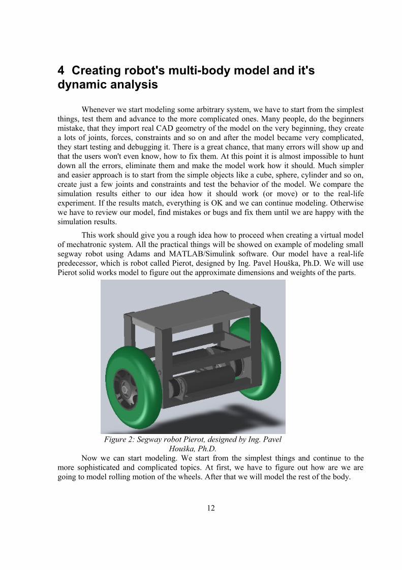
This work should give you a rough idea how to proceed when creating a virtual model of mechatronic system. All the practical things will be showed on example of modeling small segway robot using Adams and MATLAB/Simulink software. Our model have a real-life predecessor, which is robot called Pierot, designed by Ing. Pavel Houška, Ph.D. We will use Pierot solid works model to figure out the approximate dimensions and weights of the parts.

Now we can start modeling. We start from the simplest things and continue to the more sophisticated and complicated topics. At first, we have to figure out how are we are going to model rolling motion of the wheels. After that we will model the rest of the body.

12

Figure 2: Segway robot Pierot, designed by Ing. Pavel Houška, Ph.D.

4.1 Modeling of the rollingAdams does not contain any joint or constraint that would characterize rolling motion,

so we have to find a way, how to work around this problem. We can think of couple ways, how to work around the problem:

• curve-to-curve constraint

• tire

• general constraint

• general point motion

• surface contact

Not all of them works. Some works partially, some not at all. Now we will discuss individual possibilities and there advantages or disadvantages and after that we will choose one, that will suit our needs the best.

4.1.1 Curve-to-curve constraintA curve-to-curve constraint is described in [3] like this:

“A curve-curve constraint restricts a curve defined on the first part to remain in contact with a second curve defined on a second part. The curve-curve constraint is useful for modeling cams where the point of contact between two parts changes during the motion of the mechanism”

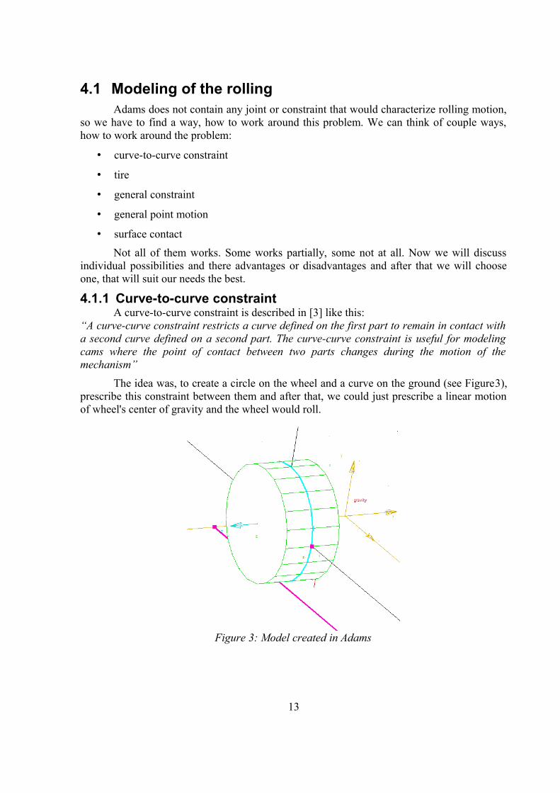
The idea was, to create a circle on the wheel and a curve on the ground (see Figure3), prescribe this constraint between them and after that, we could just prescribe a linear motion of wheel's center of gravity and the wheel would roll.

13

Figure 3: Model created in Adams

The problem is, that adams needs those two curves to have at least 4 points in common, in order to prescribe this constraint. At least, that is what error message said, when I was trying to prescribe this constraint. In our case, they have just one point in common, so this solution failed.

4.1.2 TireThis is one of the tools that adams offer. After a closer look, it was clear, that this is

way too complex solution for our problem. Description of Adams/Tire from [4] follows:

“Adams/Tire software is a module you use with Adams/Car, Adams/Chassis, Adams/Solver, or Adams/View to add tires to your mechanical model and to simulate maneuvers such as braking, steering, acceleration, free-rolling, or skidding. Adams/Tire lets you model the forces and torques that act on a tire as it moves over roadways or irregular terrain.”

It could be used for our problem, but it requires setting many parameters in order to set it up correctly. After that it would describe all the forces and torques acting on tire, but we won't need that level of accuracy, so it is not worth the effort.

4.1.3 General constraintIt is characterized by mathematical expression. Usually it is some kind of equation,

that has a zero on one side and rest of the elements on the other.In our case, we want to make rolling constant. One of the condition for rolling without slipping is, that

v=ω⋅r (1)

Where v is the translational velocity of the wheel, ω is the wheel's angular velocity and r is the wheel radius.

We have to modify this expression for use in general constraint like this:

0=v−ω⋅r (2)

This solution works quite well. If we prescribe translational velocity to the wheel or torque, it rolls without slipping, how we would expect.

4.1.4 General point motionIn this approach we prescribe rotational and translational motion at the same time and

bind them together through the equation (1). So for example, we will prescribe angular velocity and the translational velocity will be calculated from that.This is not the best approach, but it works and it could be probably used.

4.1.5 ContactIt was known, from the very beginning, that this will be the most realistic option. The

only concern was the computational time. That was the reason, why was this approach left out as the last one. In case, that the contact parameters were chosen incorrectly, we would create a system which would require a lot of computational time to solve. That would be in case we would choose high stiffness and small damping. The system would oscillate on high frequency and would be difficult to solve.

14

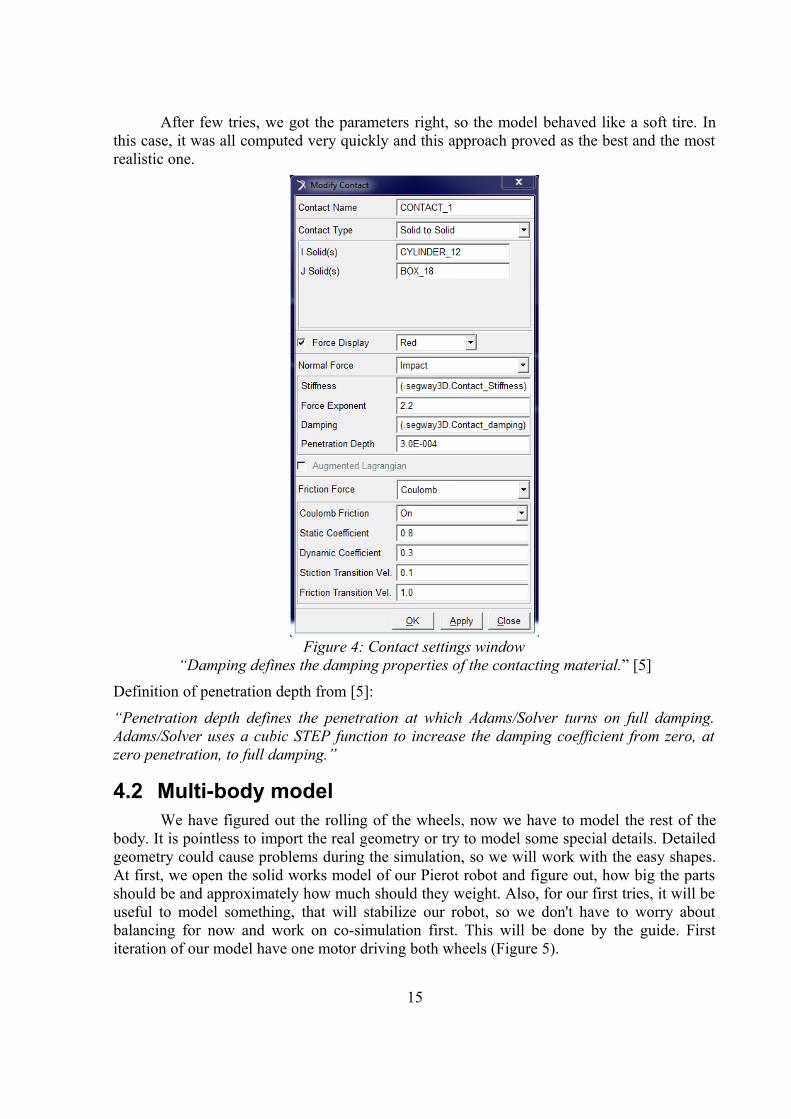
After few tries, we got the parameters right, so the model behaved like a soft tire. In this case, it was all computed very quickly and this approach proved as the best and the most realistic one.

“Damping defines the damping properties of the contacting material.” [5]

Definition of penetration depth from [5]:

“Penetration depth defines the penetration at which Adams/Solver turns on full damping. Adams/Solver uses a cubic STEP function to increase the damping coefficient from zero, at zero penetration, to full damping.”

4.2 Multi-body modelWe have figured out the rolling of the wheels, now we have to model the rest of the

body. It is pointless to import the real geometry or try to model some special details. Detailed geometry could cause problems during the simulation, so we will work with the easy shapes. At first, we open the solid works model of our Pierot robot and figure out, how big the parts should be and approximately how much should they weight. Also, for our first tries, it will be useful to model something, that will stabilize our robot, so we don't have to worry about balancing for now and work on co-simulation first. This will be done by the guide. First iteration of our model have one motor driving both wheels (Figure 5).

15

Figure 4: Contact settings window

4.2.1 Model dimensions• body

◦ width, height, length – 100 mm

◦ weight – 2 kg

• Wheel

◦ diameter – 100 mm

◦ width – 40 mm

◦ weight – 0,153 kg

• stator

◦ diameter – 29 mm

◦ length – 45 mm

◦ weight – 0,232 kg

16

Figure 5: Model with one motor

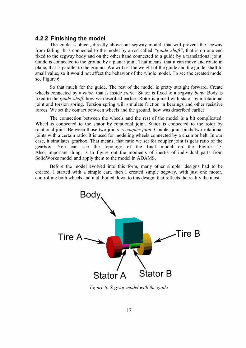
4.2.2 Finishing the modelThe guide is object, directly above our segway model, that will prevent the segway

from falling. It is connected to the model by a rod called “guide_shaft”, that is on one end fixed to the segway body and on the other hand connected to a guide by a translational joint. Guide is connected to the ground by a planar joint. That means, that it can move and rotate in plane, that is parallel to the ground. We will set the weight of the guide and the guide_shaft to small value, so it would not affect the behavior of the whole model. To see the created model see Figure 6.

So that much for the guide. The rest of the model is pretty straight forward. Create wheels connected by a rotor, that is inside stator. Stator is fixed to a segway body. Body is fixed to the guide_shaft, how we described earlier. Rotor is joined with stator by a rotational joint and torsion spring. Torsion spring will simulate friction in bearings and other resistive forces. We set the contact between wheels and the ground, how was described earlier.

The connection between the wheels and the rest of the model is a bit complicated. Wheel is connected to the stator by rotational joint. Stator is connected to the rotor by rotational joint. Between those two joints is coupler joint. Coupler joint binds two rotational joints with a certain ratio. It is used for modeling wheels connected by a chain or belt. In our case, it simulates gearbox. That means, that ratio we set for coupler joint is gear ratio of the gearbox. You can see the topology of the final model on the Figure 15.Also, important thing, is to figure out the moments of inertia of individual parts from SolidWorks model and apply them to the model in ADAMS.

Before the model evolved into this form, many other simpler designs had to be created. I started with a simple cart, then I created simple segway, with just one motor, controlling both wheels and it all boiled down to this design, that reflects the reality the most.

17

Figure 6: Segway model with the guide

5 Creation of the motor's electro-mechanical model

By electro-mechanical model we mean model of the DC motors that will drive our segway robot. We had already created the mechanical part – rotor and stator. Now, we have to figure out the parameters of the motors that will drive our robot. So we will do the dynamical analysis of the motion, to figure out the requirements on the motor. After that, we will go through motor catalogs, to choose the right one and get it's parameters. Afterwards we will create the electrical part of the model, using differential equations describing the behavior of the DC motor.

5.1 Motion analysisNow, in this section, we should analyze the desired motion of the robot, so we can choose right motor, that will be powerful enough to move with the robot in the desired way.

Now, about the motion. We don't really care, about the maximal speed. It could be 2 m/s or 5 m/s, it is not really important for our purposes. We care more about acceleration of the robot. So the acceleration should be around 1 m/s2, so the robot can balance out the tilting of it's body.

The most important motor characteristics we need to know is motor torque. We have to figure out the needed torque, so we can choose the right motor for our application.I used the equation, describing the moments acting on the motor shaft, from [6]:

M =J⋅d ω

dt+M z (3)

Where M is the moment of the motor, Mz is torque load, J is moment of inertia and ω is the angular velocity of the motor shaft.

18

Figure 7: Segway model with velocities

We will use the law of conservation of mechanical energy and we will neglect the rotational kinetic energy of the body, because it is unimportant to our problem.

12

J Rω2=

12

J W ωW2+

12

mW v2+

12

mB v2(4)

Index w is for wheel, B is for body, v is translational velocity of the wheel's center of mass. JR is reduced moment of inertia.

J R ω2=J W ωW

2+mW RW

2ωW

2+mB RW

2ωW

2 (5)

J R=J W

ωW2

ω2 +mW RW

2 ωW2

ω2 +mB RW

2 ωW2

ω2

(6)

J R=1

i 2( J W+mW RW

2+mB RW ) (7)

J =1

i2( J W +mW RW

2+mB RW )+ J m=(

1

202(2,032⋅10−4

+0,153⋅0,1+1⋅0,1)+1,29⋅10−6)kg⋅m2

Where Jm is moment of inertia of rotor

J =2.90⋅10−4 kg⋅m2

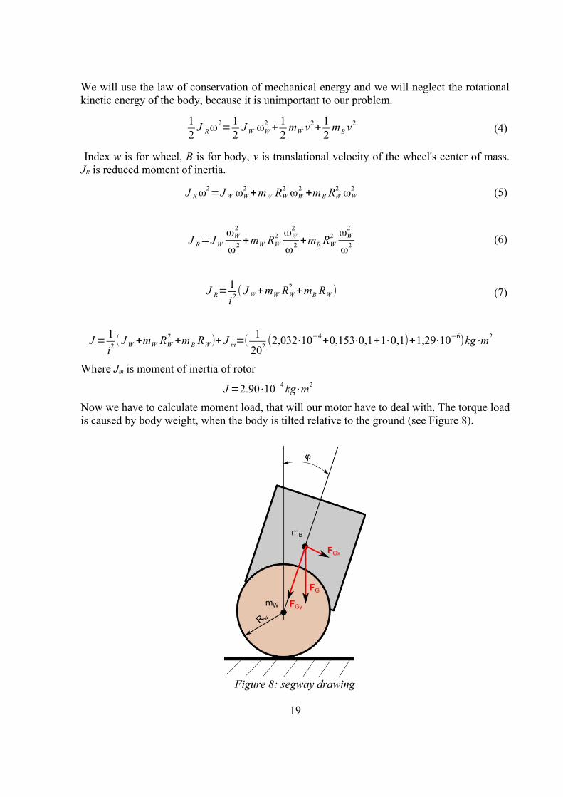
Now we have to calculate moment load, that will our motor have to deal with. The torque load is caused by body weight, when the body is tilted relative to the ground (see Figure 8).

19

Figure 8: segway drawing

M z=m⋅g⋅r⋅sinϕ=1⋅9.81⋅0.06⋅sin 20 ° Nm=0.201 Nm (8)

m is half of the body mass (the other half is covered by the second motor), r is the distance from the body center of mass to the axis of rotation

Now we go back to equation (3) and calculate desired motor torque.

M =J⋅d ω

dt+M z=J⋅a⋅RW +M z=(2.90⋅10−4

⋅1⋅0.1+0.201) Nm=0.201 Nm

So this means, that we will need a DC motor, that will deliver approximately 0,201 Nm of torque. But this estimate is very rough, we can change it afterwards. It is just useful to know, with what kinds of torques are we dealing here.

5.2 Choice of the motor and gearheadIn previous chapter we have calculated the desired torque, but we have to consider

also some other parameters of the motor. First of all, our robot is quite small, so the motor should be small as well. Size and power are directly proportional, so we would need a motor approximately around 20 W. Also the nominal voltage should be small, because we will power the motors from the batteries. The smaller the voltage, the easier it will be to supply it.

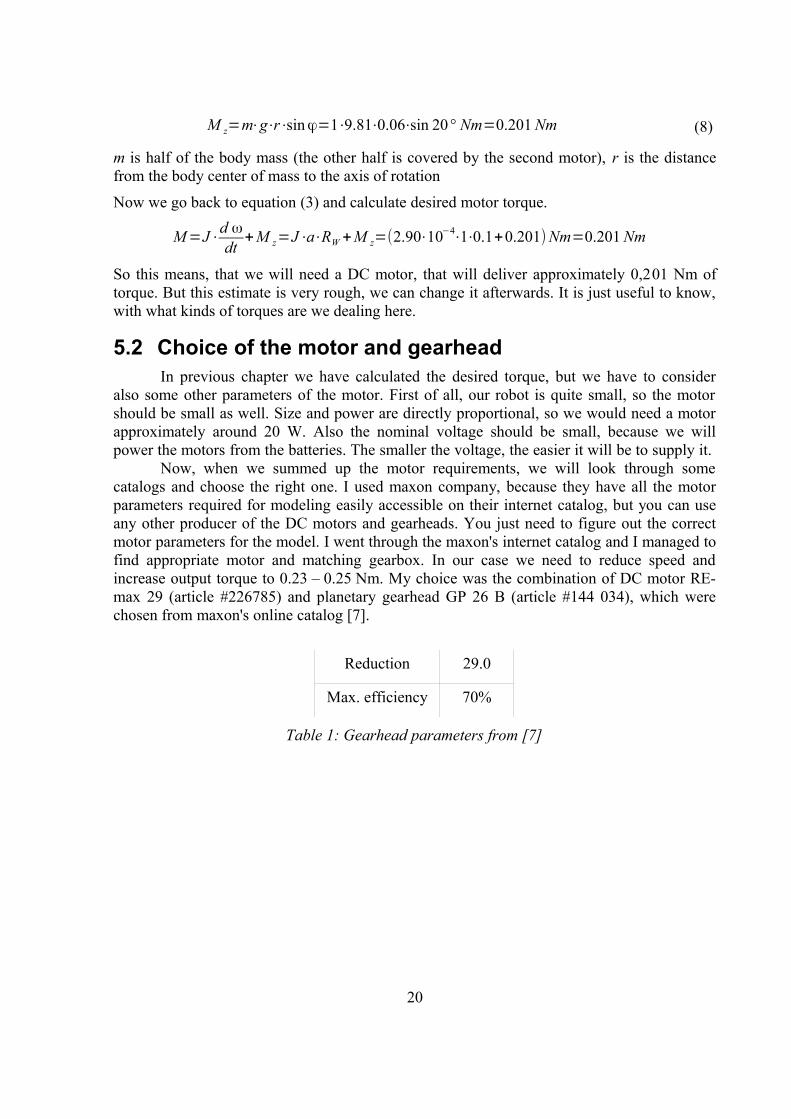
Now, when we summed up the motor requirements, we will look through some catalogs and choose the right one. I used maxon company, because they have all the motor parameters required for modeling easily accessible on their internet catalog, but you can use any other producer of the DC motors and gearheads. You just need to figure out the correct motor parameters for the model. I went through the maxon's internet catalog and I managed to find appropriate motor and matching gearbox. In our case we need to reduce speed and increase output torque to 0.23 – 0.25 Nm. My choice was the combination of DC motor RE-max 29 (article #226785) and planetary gearhead GP 26 B (article #144 034), which were chosen from maxon's online catalog [7].

Reduction 29.0

Max. efficiency 70%

Table 1: Gearhead parameters from [7]

20

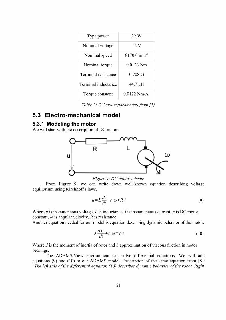
Type power 22 W

Nominal voltage 12 V

Nominal speed 8170.0 min-1

Nominal torque 0.0123 Nm

Terminal resistance 0.708 Ω

Terminal inductance 44.7 μH

Torque constant 0.0122 Nm/A

Table 2: DC motor parameters from [7]

5.3 Electro-mechanical model5.3.1 Modeling the motorWe will start with the description of DC motor.

From Figure 9, we can write down well-known equation describing voltage equilibrium using Kirchhoff's laws.

u=Ldidt

+c⋅ω+R⋅i (9)

Where u is instantaneous voltage, L is inductance, i is instantaneous current, c is DC motor constant, ω is angular velocity, R is resistance.Another equation needed for our model is equation describing dynamic behavior of the motor.

Jd ω

dt+b⋅ω=c⋅i (10)

Where J is the moment of inertia of rotor and b approximation of viscous friction in motor bearings.

The ADAMS/View environment can solve differential equations. We will add equations (9) and (10) to our ADAMS model. Description of the same equation from [8]:“The left side of the differential equation (10) describes dynamic behavior of the robot. Right

21

Figure 9: DC motor scheme

side of this equation is applied as a torque to the model of the motor. Left side is used by ADAMS/Solver automatically”

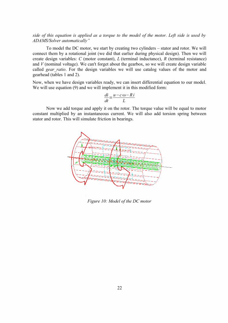
To model the DC motor, we start by creating two cylinders – stator and rotor. We will connect them by a rotational joint (we did that earlier during physical design). Then we will create design variables: C (motor constant), L (terminal inductance), R (terminal resistance) and V (nominal voltage). We can't forget about the gearbox, so we will create design variable called gear_ratio. For the design variables we will use catalog values of the motor and gearhead (tables 1 and 2).

Now, when we have design variables ready, we can insert differential equation to our model. We will use equation (9) and we will implement it in this modified form:

didt

=u−c ω−R i

L

Now we add torque and apply it on the rotor. The torque value will be equal to motor constant multiplied by an instantaneous current. We will also add torsion spring between stator and rotor. This will simulate friction in bearings.

22

Figure 10: Model of the DC motor

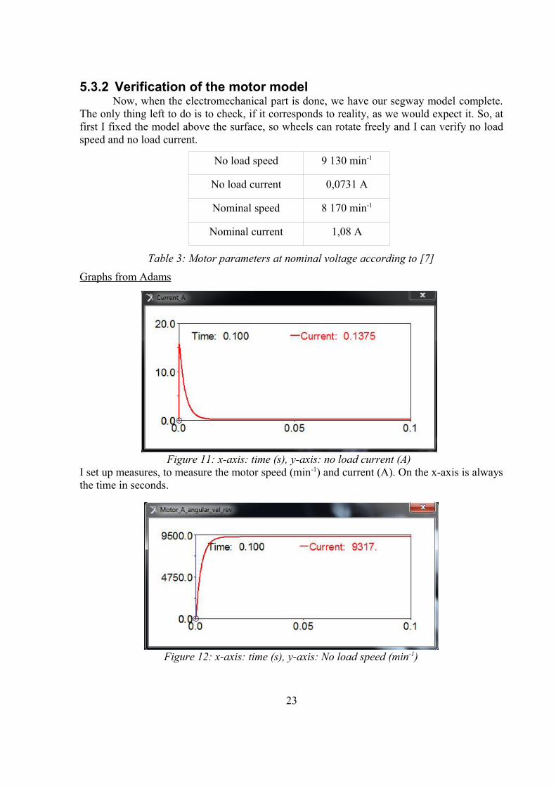
5.3.2 Verification of the motor modelNow, when the electromechanical part is done, we have our segway model complete.

The only thing left to do is to check, if it corresponds to reality, as we would expect it. So, at first I fixed the model above the surface, so wheels can rotate freely and I can verify no load speed and no load current.

No load speed 9 130 min-1

No load current 0,0731 A

Nominal speed 8 170 min-1

Nominal current 1,08 A

Table 3: Motor parameters at nominal voltage according to [7]

Graphs from Adams

I set up measures, to measure the motor speed (min-1) and current (A). On the x-axis is always the time in seconds.

23

Figure 12: x-axis: time (s), y-axis: No load speed (min-1)

Figure 11: x-axis: time (s), y-axis: no load current (A)

So, if we look at the graphs of current, they always start with the peak of 16 A approximately, which is correct and after that it drops. This behavior is expected, because at the beginning the motor have to overcome the dynamic moment to accelerate the rotor and the wheel. The speed is increasing after it gets on the stable value. That is also expected. If we compare the measured values to the catalog values they don't differ much. We have to consider, that our model is not very detailed and also the catalog values can vary depending on the individual motor.

Conclusion to the verification is, that the motor is behaving as expected. Numerical values a bit vary from catalog, but it does not indicate error in model.

24

Figure 14: x-axis: time (s), y-axis: nominal speed (min-1)

Figure 13: x-axis: time (s), y-axis: nominal current (A)

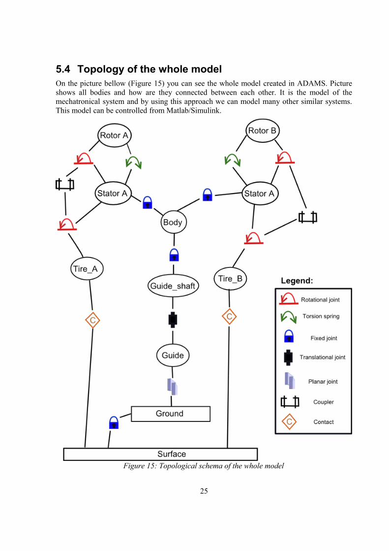
5.4 Topology of the whole modelOn the picture bellow (Figure 15) you can see the whole model created in ADAMS. Picture shows all bodies and how are they connected between each other. It is the model of the mechatronical system and by using this approach we can model many other similar systems. This model can be controlled from Matlab/Simulink.

Figure 15: Topological schema of the whole model

25

6 Co-simulation connection between Adams and Matlab/Simulink

Now is the mechanical part done. We have also created the electrical part, now we have to take care of the control of the whole system. ADAMS doesn't have any control tools, but it has toolbox ADAMS/Controls that will prepare our model for connection with other software designed for controlling. You can choose between Matlab/Simulink or MSC.Easy5. We will use co-simulation with Matlab/Simulink.

6.1 State-space modelLinear dynamic system is described by linear differential equation of order n. For

numerical solution we will re-write this equation like a system of n first order differential equations (those equations are called state equations). Now we will use the definition of state from [9]:

“State of dynamical system is described by a system of variables, called state variables. If we know values of all state variables in certain initial time t = t0 and values of input variables for t≥t 0 , we can determine the behavior of the system for time t≥t 0

We will simplify our model to just 2D problem by neglecting the second wheel, so the model won't be able to steer. Our main goal is to keep the robot from falling. To accomplish this, we will need 4 states:

• Tilt angle (angle between robot body and ground)

• Angular velocity(tilt rate – tilt angle first derivative)

• Wheels position

• Wheels velocity

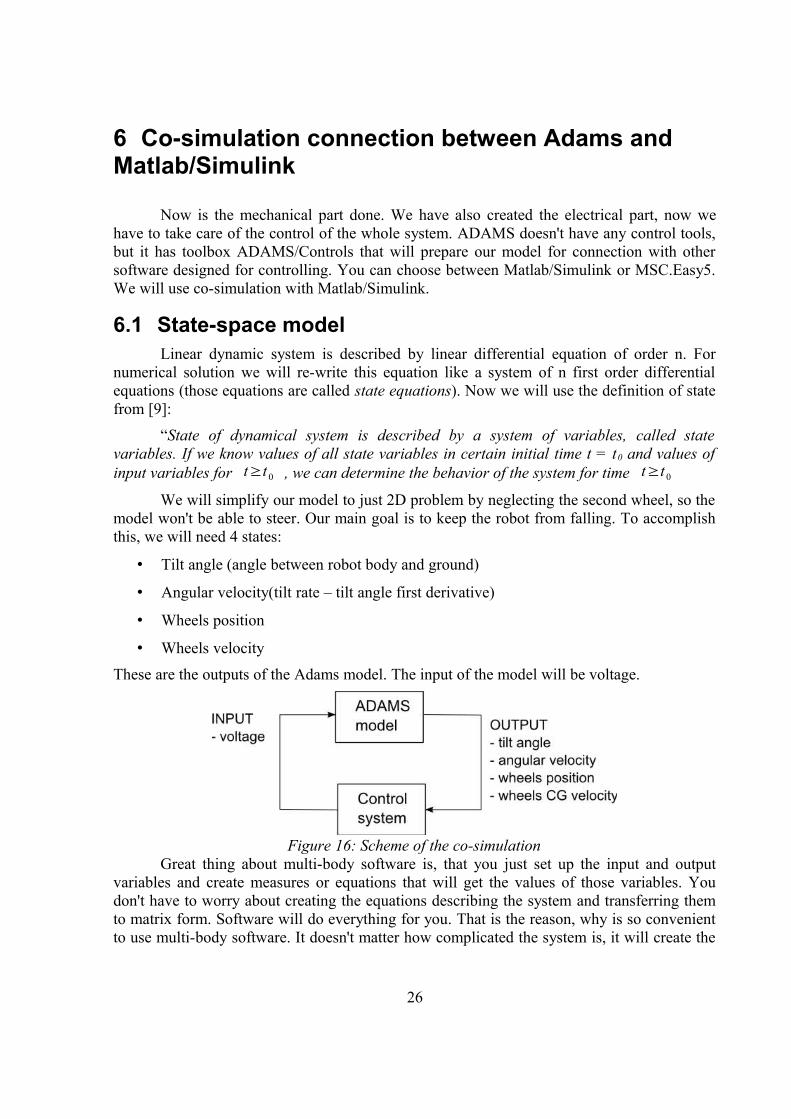
These are the outputs of the Adams model. The input of the model will be voltage.

Great thing about multi-body software is, that you just set up the input and output variables and create measures or equations that will get the values of those variables. You don't have to worry about creating the equations describing the system and transferring them to matrix form. Software will do everything for you. That is the reason, why is so convenient to use multi-body software. It doesn't matter how complicated the system is, it will create the

26

Figure 16: Scheme of the co-simulation

matrices for you and the only thing you will have to worry about, is the design and debugging of the control system.

6.2 Adams/Controls and creating the connectionNow is the time for co-simulation part. We will use Matlab for creation of the control system.

Important note! For the cooperation of MATLAB and ADAMS is important, to have compatible versions. If you have ADAMS 32-bit version, you also need MATLAB 32-bit and vice versa. Also, if you are using ADAMS 2012, it might have problems cooperating with MATLAB 2005 (versions shouldn't be too far apart). For detailed information see forums at [10] and [11].

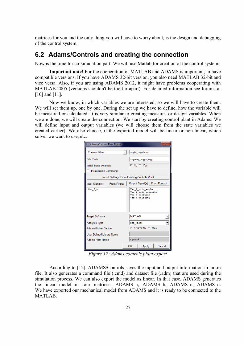
Now we know, in which variables we are interested, so we will have to create them. We will set them up, one by one. During the set up we have to define, how the variable will be measured or calculated. It is very similar to creating measures or design variables. When we are done, we will create the connection. We start by creating control plant in Adams. We will define input and output variables (we will choose them from the state variables we created earlier). We also choose, if the exported model will be linear or non-linear, which solver we want to use, etc.

According to [12], ADAMS/Controls saves the input and output information in an .m file. It also generates a command file (.cmd) and dataset file (.adm) that are used during the simulation process. We can also export the model as linear. In that case, ADAMS generates the linear model in four matrices: ADAMS_a, ADAMS_b, ADAMS_c, ADAMS_d.We have exported our mechanical model from ADAMS and it is ready to be connected to the MATLAB.

27

Figure 17: Adams controls plant export

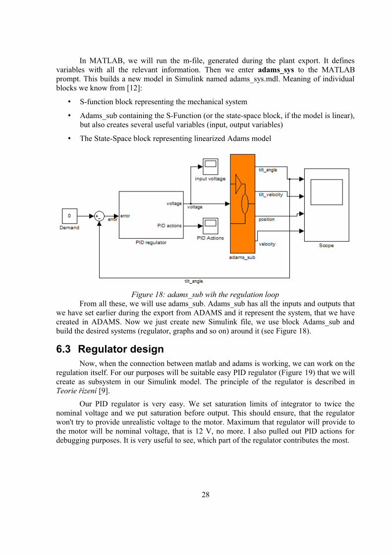
In MATLAB, we will run the m-file, generated during the plant export. It defines variables with all the relevant information. Then we enter adams_sys to the MATLAB prompt. This builds a new model in Simulink named adams_sys.mdl. Meaning of individual blocks we know from [12]:

• S-function block representing the mechanical system

• Adams_sub containing the S-Function (or the state-space block, if the model is linear), but also creates several useful variables (input, output variables)

• The State-Space block representing linearized Adams model

From all these, we will use adams_sub. Adams_sub has all the inputs and outputs that we have set earlier during the export from ADAMS and it represent the system, that we have created in ADAMS. Now we just create new Simulink file, we use block Adams_sub and build the desired systems (regulator, graphs and so on) around it (see Figure 18).

6.3 Regulator designNow, when the connection between matlab and adams is working, we can work on the

regulation itself. For our purposes will be suitable easy PID regulator (Figure 19) that we will create as subsystem in our Simulink model. The principle of the regulator is described in Teorie řízení [9].

Our PID regulator is very easy. We set saturation limits of integrator to twice the nominal voltage and we put saturation before output. This should ensure, that the regulator won't try to provide unrealistic voltage to the motor. Maximum that regulator will provide to the motor will be nominal voltage, that is 12 V, no more. I also pulled out PID actions for debugging purposes. It is very useful to see, which part of the regulator contributes the most.

28

Figure 18: adams_sub wih the regulation loop

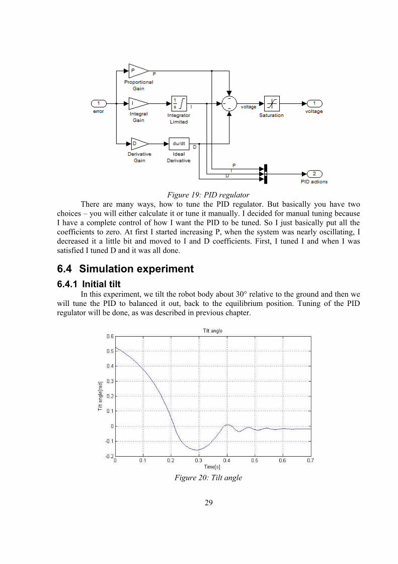
There are many ways, how to tune the PID regulator. But basically you have two choices – you will either calculate it or tune it manually. I decided for manual tuning because I have a complete control of how I want the PID to be tuned. So I just basically put all the coefficients to zero. At first I started increasing P, when the system was nearly oscillating, I decreased it a little bit and moved to I and D coefficients. First, I tuned I and when I was satisfied I tuned D and it was all done.

6.4 Simulation experiment6.4.1 Initial tilt

In this experiment, we tilt the robot body about 30° relative to the ground and then we will tune the PID to balanced it out, back to the equilibrium position. Tuning of the PID regulator will be done, as was described in previous chapter.

29

Figure 19: PID regulator

Figure 20: Tilt angle

30

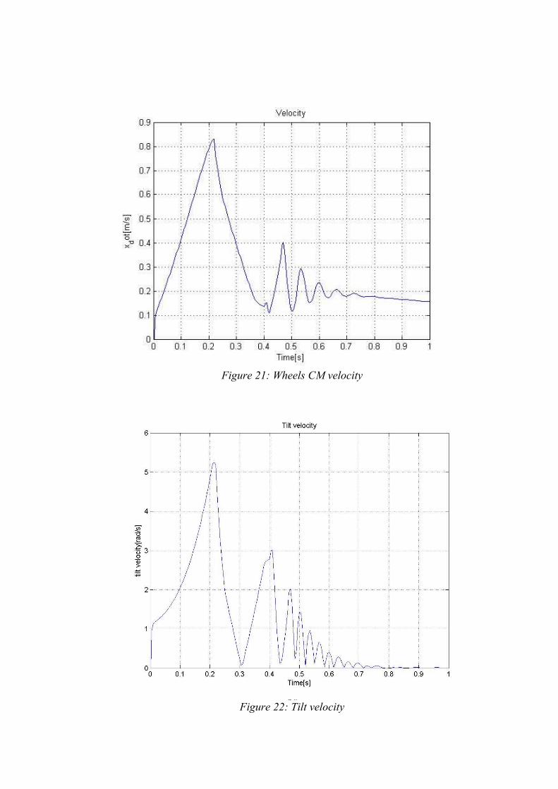
Figure 21: Wheels CM velocity

Figure 22: Tilt velocity

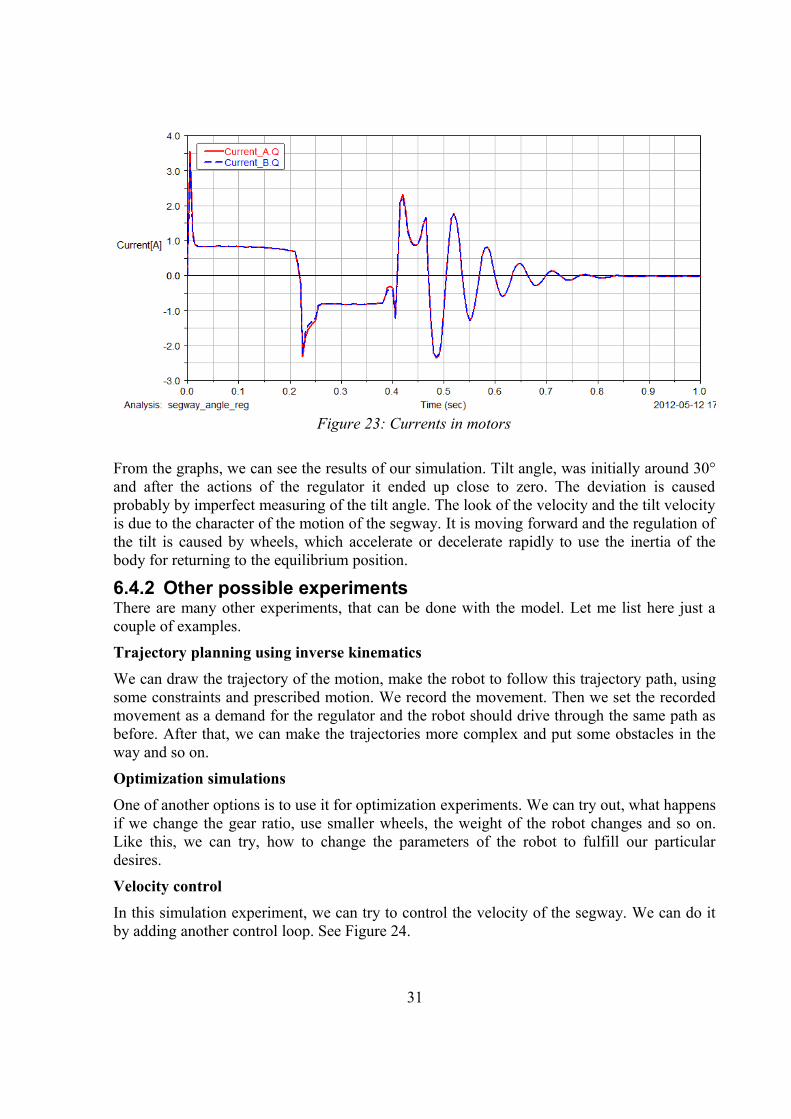
From the graphs, we can see the results of our simulation. Tilt angle, was initially around 30° and after the actions of the regulator it ended up close to zero. The deviation is caused probably by imperfect measuring of the tilt angle. The look of the velocity and the tilt velocity is due to the character of the motion of the segway. It is moving forward and the regulation of the tilt is caused by wheels, which accelerate or decelerate rapidly to use the inertia of the body for returning to the equilibrium position.

6.4.2 Other possible experimentsThere are many other experiments, that can be done with the model. Let me list here just a couple of examples.

Trajectory planning using inverse kinematics

We can draw the trajectory of the motion, make the robot to follow this trajectory path, using some constraints and prescribed motion. We record the movement. Then we set the recorded movement as a demand for the regulator and the robot should drive through the same path as before. After that, we can make the trajectories more complex and put some obstacles in the way and so on.

Optimization simulations

One of another options is to use it for optimization experiments. We can try out, what happens if we change the gear ratio, use smaller wheels, the weight of the robot changes and so on. Like this, we can try, how to change the parameters of the robot to fulfill our particular desires.

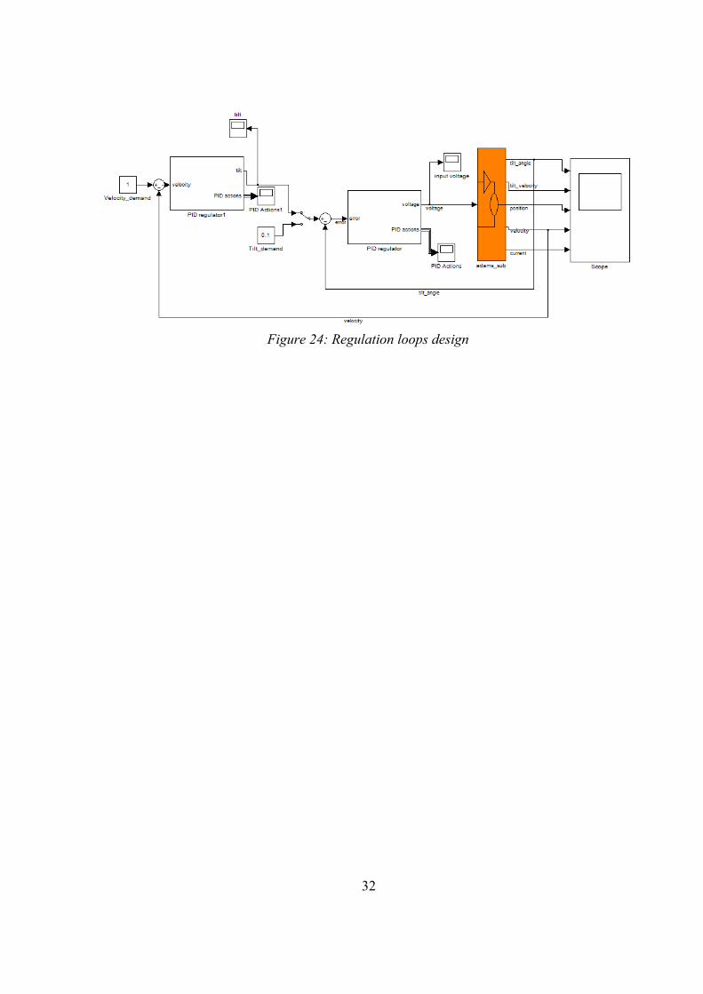
Velocity control

In this simulation experiment, we can try to control the velocity of the segway. We can do it by adding another control loop. See Figure 24.

31

Figure 23: Currents in motors

32

Figure 24: Regulation loops design

7 Conclusion

This work included a lot of struggling with software and making it work. Also a lot of struggling with model, finding errors, debugging and making it work in at least in a bit realistic way. We have created the multibody model of the robot and we have done it's dynamic analysis. Based on this analysis we have chosen the right DC motor and gearhead for the robot. After that we have created working co-simulation link between multibody model and the control system in Simulink. The result is working model of segway robot, that used the best of ADAMS and Simulink. We also verified and tried out the behavior of our model during a simulation experiments. There is still a plenty of things to develop or improve. The model can be further developed with complicated path planning and control systems, so it can accomplish more advanced tasks.

33

8 References

[1] GARCÍA DE JALÓN, J., BAYO, E.: Kinematic and Dynamic Simulation of Multibody Systems: The Real-Time challenge. New-York: Springer-Verlag, 1994. ISBN 0-387-94096-0. Available from: http://mat21.etsii.upm.es/mbs/bookPDFs/bookGjB.htmhttp://mat21.etsii.upm.es/mbs/bookPDFs/bookGjB.htm

[2] Adams for Multibody Dynamics. [online]. [cit. 2012-05-22]. Available from: http://www.mscsoftware.com/Products/CAE-Tools/Adams.aspx [3] Adams/Constraints. [online]. [cit. 2012-03-19]. Available from: http://www.kxcad.net/msc_software/adams_md_r2/adams_view/building_models_constraints.pdf

[4] Adams/Tire, [online]. [2012-03-10]. Available from: http://www.kxcad.net/msc_software/adams_md_r2/adams_tire/tire_welcome.pdf

[5] , Adams/Solver, [online]. [2012-03-13] Available from: http://simcompanion.mscsoftware.com/infocenter/index?page=content&id=DOC9804&cat=MD_2011_ADAMS_DOCS&actp=LIST

[6] KOLÁČNÝ, J.: Elektrické pohony [online]. [cit. 2012-04-18]. Available from: http://www.umel.feec.vutbr.cz/VIT/images/pdf/studijni_materialy/bc/elektricke_pohony_%20S.pdf

[7] Maxon motor catalog. [online]. [cit. 2012-04-15]. Available from: http://www.maxonmotor.com/maxon/view/catalog

[8] BŘEZINA, T., HADAŠ,Z., VETIŠKA, J., Using of Co-simulation ADAMS-SIMULINK for Development of Mechatronic Systems. 14Th INTERNATIONAL CONFERENCE ON MECHATRONICS. Trenčín, AD University of Trencin. 2011.

[9] Skalický, J.: Teorie řízení 1,VUT v Brně, Brno, 2002

[10] MSC software corporation. [online]. [cit. 2012-03-22]. Available from: www.mscsoftware.com

[11] MathWorks – MATLAB and Simulink for Technical Computing [online]. [cit. 2012-03-22]. Available from: www.mathworks.com

[12]: Getting started using ADAMS, [online]. [2012-03-31]. Available from: http://simcompanion.mscsoftware.com

34

9 Annexes

9.1 Adams model.zipsegway3D.bin - model of segway in Adamssegway3D_angle.bin - model of tilted segway used for initial tilt experimentgraphing.m - m-file used for graphing the results of the simulationregulator_PID.mdl - regulator v Simulinkusegway_angle_reg.m - m-file with the necessary parameters for co-simulation

35