Embed Size (px)
DESCRIPTION
Cointegration is an common phenomena in time series data. The material is about some testing procedure for cointegration, namely Augumented Dicky Fuller Test, ARS test.
Citation preview
ECON3350/7350COINTEGRATION
Alicia N. Rambaldi
Week 6
1 / 28

In this lecture
Readings
IntroductionSpurious Regression vs Cointegration
Spurious Regression
CointegrationIntroduction to CointegrationDefinition of CointegrationCointegration OrderExampleTesting for CointegrationProperties of the OLS estimator in the case of cointegration.Testing the cointegration spaceNon-Uniqueness of �
Coming Up
2 / 28

Reference Materials
Author Title Chapter Call No
Enders, W AppliedEconometricTime Series,
3e
6.1-6.2
HB139 .E552015
Verbeek, M A Guide toModern
Econometrics
9.2,9.3 HB139.V465 2012
3 / 28
Spurious Regression vs Cointegration
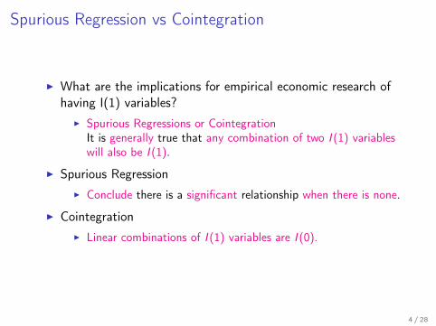
I What are the implications for empirical economic research ofhaving I(1) variables?
I Spurious Regressions or CointegrationIt is generally true that any combination of two I (1) variableswill also be I (1).
I Spurious RegressionI Conclude there is a significant relationship when there is none.
I CointegrationI Linear combinations of I (1) variables are I (0).
4 / 28

Spurious Regression
I Assume xt
= xt�1
+ ✏x ,t and y
t
= yt�1
+ ✏y ,t where ✏
x ,t and✏y ,t are independent white noise.
I Clearly there is no relationship between xt
and yt
.I If we do not know the above and wish to ’test’ for a
relationship between xt
and yt
, we would normally estimate
yt
= ↵̂+ �̂xt
+ et
I and use a t � test to test
H0 : � = 0 against H1 : � 6= 0
If xt
and yt
were I (0), �̂ would be approximately Normal, twould be approximately Student � t or at leastT
12
⇣�̂ � �
⌘! N(0,V ).
5 / 28

Spurious Regression (cont.)
I But as xt
and yt
are I (1), the distribution of �̂ is moredisperse than Normal and the distribution of t is more dispersethat Student�t.
P(|t| > 1.96) = P(Rejected H0
) > 0.05
I Implications: Tend to reject H0
too oftenI What happens as T ! 1?
I Things get worse and there is no well defined asymptoticdistribution to which �̂ converges:
T12 (�̂ � �) ! 1 and P(|t| > 1.96) increases
6 / 28

Spurious Regression (cont.)
I Indications of a Spurious regression:Signicant t � values; Respectable (sometimes high) R2; lowDurbin-Watson (DW) statistics.
I The signicant t - values occur because the random walks tendto wander, and this wandering looks like a trend.
I If they wander in the same direction for a while (say for thetime of the observed sample), there appears to be arelationship.
I In:I y
t
= ↵+ �xt
+ ✏t
; ✏t
⇠ I (1) so the regression is meaningless.I This explains why DW is low.
7 / 28

Cointegration
I Recall the concept of the stochastic trend
st
= st�1
+ ⌘t
where ⌘t
⇠ I (0)
Any linear combination of st
will be I (1).I Thus if
xt
= ast
+ ⌫x ,t where ⌫
x ,t ⇠ I (0) then xt
⇠ I (1)
8 / 28

Common Stochastic TrendI How can two I (1) variables combine to form an I (0) variable?
I Recall
xt
= ast
+ ⌫x ,t where ⌫
x ,t ⇠ I (0) so xt
⇠ I (1)I Now assume
yt
= st
+ ⌫y ,t where ⌫
y ,t ⇠ I (0) so yt
⇠ I (1)I Then
xt
� ayt
= (ast
+ ⌫x ,t)� a(s
t
+ ⌫y ,t)
= ast
+ ⌫x ,t � as
t
� a⌫y ,t
= ⌫x ,t � a⌫
y ,t which is I (0)
I This is a case of cointegration.I The variables share a common stochastic trend: s
t
.9 / 28

Cointegration and Equilibrium
I The economic interpretation and signicance of cointegrationI We may regard the cointegrating relation
zt
= xt
� ayt
as a stable equilibrium relation.I Although x
t
and yt
are themselves unstable as they are I (1),they are attracted to a stable relationship that exists betweenthem, z
t
⇠ I (0).I For example, there is strong evidence that interest rates are
I (1). But the spread between two rates of different maturities,within the same market, appear to be I (0).
10 / 28

Common Stochastic TrendExample
CWTB3Y: Augmented Dickey-Fuller test statistic -1.253373, p-value (0.6433)
CWTB5Y: Augmented Dickey-Fuller test statistic -1.199108, p-value(0.6673)
SPREAD: Is it I (0)? We return to this question.
The expectations theory of the term structure of interest rateswould suggest that if the interest rates themselves are I (1), thespread between rates of different maturity will be I (0) (Campbelland Shiller,1991).
11 / 28

Definition of Cointegration
I It is possible for a cointegrating relation to involve manyvariables. That is, w
t
may be a (n ⇥ 1) vector. Also wt
maybe integrated of order d .
I A more formal definition of cointegration (Engle & Granger,1987):
Definition
The components of the vector wt
are said to be cointegrated oforder d , b, denoted CI (d , b), if(i) all components of w
t
are I (d),(ii) there exists a vector (� 6= 0) so that
zt
= �0wt
⇠ I (d � b), b > 0
The vector � is called the cointegrating vector.
12 / 28

Cointegration OrderI If w
t
= (w1,t ,w2,t , ...,wn,t)0 ⇠ I (1) but
w 0t
� ⇠ I (0)
I where
�0wt
= w1,t�1 + w2,t�2 + ...wn,t�n
= (�1,�2, ...,�n
)0
0
BBB@
w1,tw2,t
...wn,t
1
CCCA
I Then we say that components of the vector wt
arecointegrated of order 1, 1, denoted CI (1, 1).
I In our simple example above,
wt
=
✓xt
yt
◆and � =
✓1�a
◆
I because xt
� ayt
⇠ I (0).13 / 28

Example
King, R.G., C.I. Plosser, J.H. Stock, and M.W. Watson (1991)."Stochastic trends and economic fluctuations." The American
Economic Review, 81,819-840.
Yt
= �t
K ✓t
L1�✓t
yt
= ln(�t
) + ✓kt
+ (1 � ✓)lt
ln(�t
) = ln(�t�1
) + ✏t
Income = f (Capital , Labour) with technology/productivity shocks�t
14 / 28

Example
(cont.)The economy’s resource constraint implies that output is eitherconsumed or invested, Y
t
= Ct
+ It
, and with common stochastic
trends (�t
) the ratiosCt
Yt
andIt
Yt
(the Great Ratios) are stable.
Therefore, in logs, ct
� yt
and it
� yt
must be I (0) and ct
, yt
, andit
are I (1) but cointegrate.That is
�0wt
=
✓1 0 b
1
0 1 b2
◆0
@ct
it
yt
1
A =
✓ct
+ b1
yt
it
+ b2
yt
◆⇠ I (0)
We also know from the theory that we can restrict b1
= �1 andb2
= �1.
15 / 28

Testing for Cointegration
I Recall that if a vector of I (1) variables do not cointegrate,then no combination of them will be I (0). However, if a vectorof I (1) variables DO cointegrate, then there is a combinationof them that will be I (0).
I Simple solution: to test for cointegration.I Consider the case of three variables: x
t
, yt
, and zt
I Estimate: xt
= ↵̂+ �̂1yt + �̂2zt + et
(by OLS)I Test the residual, e
t
, for a unit root. If et
⇠ I (0), thenxt
, yt
, and zt
cointegrate.
I There are a number of ways we could perform this test. Wewill look at using the Dickey-Fuller test statistic and theDurbin-Watson statistic.
16 / 28

Testing for Cointegration (cont.)
I Because the residual et
comes from a potential cointegratingrelation, the test statistics will not have the usual distributionsso we cannot use the same critical values.
I In both tests we assume et
= ⇢et�1
+ ⌫t
(⌫t
is WN) and testH
0
: ⇢ = 1.I The Augmented Dickey-Fuller test to test for cointegration.
We proceed as usual but use critical values from Table C inEnders.
I The Durbin-Watson test to test for cointegration (CRDW).We proceed as usual but use critical values from Table 9.3 inVerbeek.
17 / 28

Example
Expectations theory of the term structure of interest rates impliesthe following empirically testable feature
If i3y ,t ⇠ I (1) then i
5y ,t ⇠ I (1) and i5y ,t � i
3y ,t ⇠ I (0)
I That is, the long and short interest rates will cointegrateI We had computed:
i3y ,t : Augmented Dickey-Fuller test statistic -1.253373, p-value (0.6433)i5y ,t : Augmented Dickey-Fuller test statistic -1.199108, p-value(0.6673)Thus, they are I (1)
I i5y ,t � i
3y ,t
I H0 : et
= i5y ,t � i3y ,t ⇠ I (1) ,I That is, the long and short interest rates will cointegrate and
we know the cointegrating relation is � = (1,�1).
18 / 28

Residual Based Dickey Fuller Test (cont.)I For now, we will ignore the fact we know and let it be
estimated as � = (1,�b), so we are only going to test the firstpart of the theory, i.e., that the two interest rates cointegrate.
Example
We estimate with T = 48
i5y ,t = 0.798116 + 0.945139i
3y ,t + et
�et
= �0.398300et�1
+ ⌫̂t
(0.116301)
I Augmented Dickey-Fuller test statistic= -3.424726I Critical value from Table C is -3.46 (at the 5% level) and -3.13
(at the 10%)I Therefore, we marginally reject the null hypothesis and
conclude there is some evidence to support the Expectationstheory.
19 / 28

Residual Based CRDW
I If the first order autocorrelation is one (⇢ = 1) then theDW ! 0. Thus, the DW of the cointegrating regression goesto zero under the null hypothesis
Example
We estimate with T = 48
i5y ,t = 0.798116 + 0.945139i
3y ,t + et
DW = CRDW = 1.654472
I At the 5% the critical value (Table 9.3 in Verbeek) is 0.72 andthus we reject H
0
: et
⇠ I (1) and conclude there is evidence forthe Expectations theory of the term structure of interest rates.
20 / 28

Properties of the OLS estimator in the case of cointegrationI The OLS estimator �̂ = (↵̂, �̂
1
, �̂2
)0.I In the case of cointegration, the OLS estimator of � will be
superconsistent.I That is, although normal OLS estimates converge to N(0,V )
at the rate T12 , the OLS estimate of a cointegrating vector
converges at the rate T .
I Normally,
⇣�̂ � �
⌘! 0 and T
12
⇣�̂ � �
⌘! N(0,V )
I With cointegration
⇣�̂ � �
⌘! 0 and T
12
⇣�̂ � �
⌘! 0
T⇣�̂ � �
⌘! N(0,V )
21 / 28

Testing the cointegrating space when there is onecointegrating vector
Recall that the Expectations theory of the term structure of interestrates implied
i3y ,t ⇠ I (1) then i
5y ,t ⇠ I (1) and i5y ,t � i
3y ,t ⇠ I (0)
Put another way, if i3y ,t ⇠ I (1) then i
5y ,t ⇠ I (1) because theyshare a common stochastic trend AND the cointegrating vector forthe cointegrating relation is � = (1,�1)0.
I Thus we can test the evidence in support of this theory bysimply calculating z
t
= i5y ,t � i
3y ,t and then testing zt
⇠ I (0)with a simple ADF.
I If we Reject the null hypothesis of a unit root in zt
, then ifi5y ,t ⇠ I (1), then it must hold that i
3y ,t ⇠ I (1) because theyshare a common stochastic trend and the cointegrating vectoris � = (1,�1)0
22 / 28

Testing the more explicit economic theories
Assume wt
=
0
@ct
yt
at
1
Aconsumption
incomewealth (assets)
I If we have a theory that says the cointegrating space is completelyknown, e.g., � = (1,�1,�1)0 say, then we can test the evidence insupport of this theory by constructing the variable z
t
= �0wt
anddoing a test for z
t
⇠ I (1) against zt
⇠ I (0).
Examples
Permanent income hypothesis says
zt
= ct
-yt
= ( 1 �1 )
✓ct
yt
◆⇠ I (0).
I To test this we test for stationarity of zt
(with a simple ADF test).If there is evidence of any form of nonstationarity then this can betaken as evidence against the theory.
23 / 28

The cointegrating space is partially known
I Let the income consumption relation respond to levels ofwealth, e.g., � = (1,�1,�b)0 say, then
I We can test the evidence in support of this theory by
constructing the variable z1,t = (1,�1)0
✓ct
yt
◆= c
t
� yt
and
regressing z1,t on a
t
.
z1,t = µ̂+ b̂a
t
+ et
I Then test for stationarity of et
. If using ADF, useCointegrating ADF statistics with, in this case, two variables.-Table C Enders.
I Note that µ̂ can be interpreted as the mean of the error
correction term zt
.
24 / 28

Non-Uniqueness of �
Recall cointegration with stochastic trend st
where wt
= (xt
, yt
)0
xt
= ast
+ ⌫x ,t where ⌫
x ,t ⇠ I (0) so xt
⇠ I (1) andyt
= st
+ ⌫y ,t where ⌫
y ,t ⇠ I (0) so yt
⇠ I (1)
Then,
�0wt
= (1,�a)0✓
xt
yt
◆
= xt
� ayt
= ⌫x ,t � a⌫
y ,t which is I (0)
Here � = (1,�a)0 because this combination cancelled thestochastic trends.
25 / 28

Non-Uniqueness of � (cont.)
I However,I if 2� = (2,�2a)0 or � = (1,�a)0 for any kappa 6= 0 will also
work as �0wt
⇠ I (0).
�0wt
= (2,�2a)0✓
xt
yt
◆
= 2(xt
� ayt
)
= 2(⌫x ,t � a⌫
y ,t) which is I (0)
I Thus we normalise, � = (1,�a)0 to make � unique.
26 / 28

Example
in the Real Business Cycle model with Balanced Growth Hypthesis(King et al.,1991) we had three variables (c
t
, it
, yt
) and onecommon stochastic trend - productivity shocks.
I Thus, there are n = 3 variables, and n � r = 1 commonstochastic trends. Therefore, r = 2, cointegrating vectors:
� =
2
41 00 1b1
b2
3
5
I Although much emphasis is placed upon estimating thecointegrating vectors, except where r = 1, these vectors arenot interpretable as they are not unique.
I What is unique is the cointegrating space. The cointegratingvectors span (lie in) the cointegrating space.
27 / 28

Coming Up
ARCH, GARCH, Stochastic Volatility and Realised volatility. Testsfor ’ARCH-type’ errors and model identification.
28 / 28


![VQLWRFXGH5 GDR/VXURKSVRK3 - IN.gov+2 kshvr- w6 v\ud0 w6 hh pxd0uhss8 hl]odjx$ l pld0wdhu*uhss8 l pld0wdhu*uhzr/ uhwdzlhwk : \uhkjxd/ lrk2ohglg0 kvded :uhss8 lhqr podd6 dzhlqvlvvlv0](https://img.pdfslide.tips/doc/110x75/60c82cc510b34f01b47e087b/vqlwrfxgh5-gdrvxurksvrk3-ingov-2-kshvr-w6-vud0-w6-hh-pxd0uhss8-hlodjx-l.jpg)