Well-known shortcomings,advantages and

computational challengesin Bayesian modelling:

a few case storiesOle Winther

The Bioinformatics CenterUniversity of Copenhagen

Informatics and Mathematical ModellingTechnical University of Denmark

DK-2800 Lyngby, Denmarkole.winther@gmail.com

owi@imm.dtu.dk

1

Overview

1. How many species? predicting sequence tags.

• Non-parametric Bayes

• Averaging beats maximum likelihood

• The model is always wrong (and Bayes can’t tell)

2. Computing the marginal likelihood with MCMC

• Motivation: computing corrections to EP/C

• The trouble with Gibbs sampling

• Gaussian process classification

2

How many species?

3

DNA sequence tags - CAGE

4

Look at the data - cerebellum

5 10 15 20 25 300

200

400

600

800

1000

1200

1400

1600

1800

m(n

)

n200 400 600 800 1000 1200

0

10

20

30

40

50

60

m(n

)

n

5

Look at the data - embryo

5 10 15 20 25 300

200

400

600

800

1000

1200

1400

1600

1800

2000

m(n

)

n5000 10000 15000

0

10

20

30

40

50

60

m(n

)

n

6

Chinese restaurant process - Yor-Pitmansampling formula

Observing new species given counts n = n1, . . . , nk in k bins:

p(n1, . . . , nk,1|n, σ, θ) =θ + kσ

n + θwith

k∑i=1

ni = n

Re-observing j:

p(n1, . . . , nj−1, nj + 1, nj+1, . . . , nk|n, σ, θ) =nj − σ

n + θ

Exchangeability – invariant to re-ordering

E, E, M, T, T : p1 =θ

θ

1− σ

1 + θ

θ + σ

2 + θ

θ + 2σ

3 + θ

1− σ

4 + θ

M, T, E, T, E : p2 =θ

θ

θ + σ

1 + θ

θ + 2σ

2 + θ

1− σ

3 + θ

1− σ

4 + θ= . . . = p1

7

Inference and prediction

Likelihood function, e.g. E, E, M, T, T

p(n|σ, θ) =θ

θ

1− σ

1 + θ

θ + σ

2 + θ

θ + 2σ

3 + θ

1− σ

4 + θ

=1∏n−1

i=1(i + θ)

k−1∏j=1

(θ + jσ)k∏

i′=1

ni′−1∏j′=1

(j′ − σ)

Flat prior distribution for σ ∈ [0,1] and θ pseudo-count parameter.

Predictions for new count m:

p(m|n) =∫

p(m|n, σ, θ) p(σ, θ) dσdθ

with Gibbs sampling (σ, θ) and Yor-Pitman sampling for m.

8

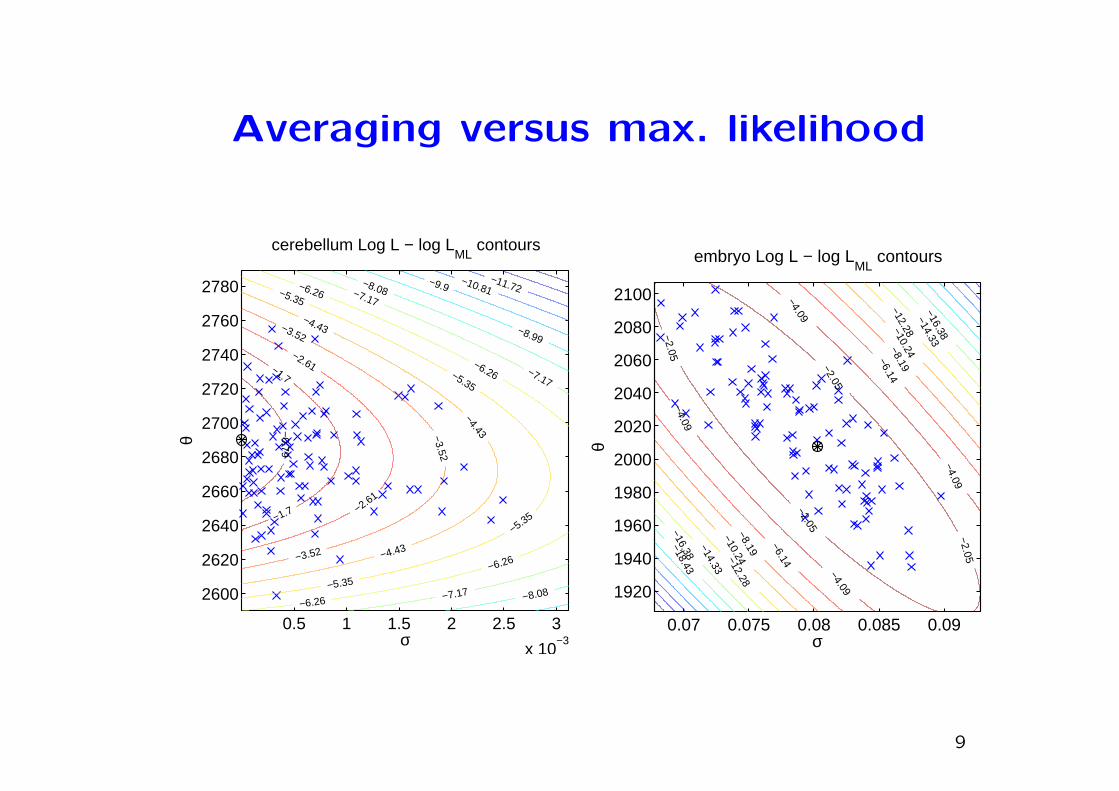
Averaging versus max. likelihood

0.5 1 1.5 2 2.5 3

x 10−3

2600

2620

2640

2660

2680

2700

2720

2740

2760

2780−11.72

−10.81−9.9

−8.99

−8.08

−8.08

−7.17

−7.17

−7.17−6.26

−6.26

−6.26

−6.26

−5.35

−5.35

−5.35

−5.35

−4.43

−4.43

−4.43

−3.52

−3.52

−3.52

−2.61

−2.61

−1.7

−1.7

−0.79

cerebellum Log L − log LML

contours

σ

θ

0.07 0.075 0.08 0.085 0.09

1920

1940

1960

1980

2000

2020

2040

2060

2080

2100

−18.43−16.38

−16.38

−14.33

−14.33

−12.28

−12.28

−10.24

−10.24

−8.19

−8.19

−6.14

−6.14−4.09

−4.09

−4.09

−4.09

−2.05

−2.05

−2.05

−2.05

embryo Log L − log LML

contours

σ

θ

9

Notice anything funny?

2 4 6

x 105

0

5000

10000

15000

n

k

cerebellum

1.15

1.2

x 104

93509400945095009550

18625714201440146014801500

10

Notice anything funny? Example 2

2 4 6 8 10 12

x 105

0

2000

4000

6000

8000

10000

12000

14000

16000

n

k

embryo

1.3

1.35

1.4x 10

4

1.021.041.061.08x 10

4

3447941750

1800

1850

11

(Well-known) take home messages

• Parameter averaging works!

• The model is always wrong! (as revealed with sufficient data)

• Only one model considered!

• What happened to being Bayesian about model selection?

12

Calculating the marginal likelihood

The marginal likelihood:

p(D|H) =∫

p(D|f ,H) p(f |H) df

Approximate inference needed!

Monte Carlo: slow mixing, non-trivial to get marginal likelihood

estimates

Expectation propagation+, variational Bayes, loopy BP+: some-

times not precise, approximation errors not controllable, not appli-

cable to all models.

13

Motivation: validating EP corrections

Kuss-Rasmussen (JMLR 2006) N = 767 3-vs-5 GP USPS digit

classification with

K(x,x′) = σ2 exp

(−||x− x′||2

2`2

)I: logR = logZEPc − logZEP and II+III: logZMCMC − logZEP.

0.00010.001

0.001

0.01

0.01

0.01

0.1

0.1

0.1

0.1

0.2

0.2

0.2

0.2

0.30.3

0.3

0.3

0.3

0.3

0.40.4

0.4

0.4

0.4

0.50.5

0.5

0.5

0.60.6

0.6

log lengthscale, ln(`)

log

magnit

ude,

ln(σ

)

1.5 2 2.5 3 3.5 4 4.5 5

0

0.5

1

1.5

2

2.5

3

3.5

4

4.5

5

0.0001

0.001

0.001

0.01

0.01

0.01

0.1

0.1

0.1

0.1

0.2

0.2

0.2

0.2

0.3

0.4

log lengthscale, ln(`)

log

magnit

ude,

ln(σ

)

1.5 2 2.5 3 3.5 4 4.5 5

0

0.5

1

1.5

2

2.5

3

3.5

4

4.5

5

1e−07

1e−07

1e−0

7

1e−07

1e−07

1e−07

1e−0

7

1e−07

1e−07

1e−07

1e−07

1e−07

1e−07

1e−07

1e−07

1e−07

1e−07

1e−07

1e−07

1e−07

1e−07

1e−

07

1e−07

1e−0

71e

−07

1e−0

7

1e−0

7

1e−07

1e−0

7

1e−07

1e−0

7

1e−07

1e−0

7

1e−07

1e−07

1e−07

1e−07

1e−06

1e−06

1e−0

6

1e−06

1e−06

1e−06

1e−0

6

1e−06

1e−06

1e−06

1e−06

1e−06

1e−06

1e−06

1e−06

1e−06

1e−0

6

1e−06

1e−06

1e−0

6

1e−06

1e−06

1e−06

1e−0

6

1e−0

6

1e−06

1e−

06

1e−06

1e−0

6

1e−06

1e−06

1e−06

1e−06

1e−06

1e−06

1e−06

1e−06

1e−06

0.0001 0.0001

0.0001

0.0001

0.0001

0.0001

0.0001

0.0001

0.0001

0.0001

0.0001

0.0001

0.0001

0.0001

0.0001

0.0001

0.00

01

0.00

01

0.0001

0.00

01

0.0001

0.0001

0.0001

0.0001

0.0001

0.00

01

0.0001

0.0001

0.00010.0001

0.00

01

0.00

01

0.0001

0.00

01

0.001

0.001 0.001

0.00

1

0.001

0.001

0.001

0.001

0.001

0.001

0.001

0.001

0.00

1

0.001

0.001

0.001

0.001

0.001

0.001

0.00

1

0.001

0.001

0.001

0.001

0.001

0.00

1

0.00

1

0.001

0.00

1

0.001

0.001

0.001

0.001

0.001

0.001

0.001

0.001

0.01

0.01 0.01

0.01

0.01

0.01 0.

01

0.01

0.01

0.01

0.01

0.01

0.01

0.01

0.01

0.01

0.01

0.01

0.01

0.01

0.01

0.01

0.01

0.01

0.01

0.01

0.01

0.01

0.01

0.01

0.01

0.010.01

0.01

0.01

0.01

0.01

0.01

0.01

0.01

0.01

0.1

0.1

0.1 0.1

0.1

0.1

0.1

0.10.1

0.1

0.1

0.1

0.1

0.1

0.1

0.1

0.1

0.1

0.10.1

0.1 0.1

0.1

0.1

0.1

0.1

0.1

0.1

0.1

0.1

0.1

0.1

0.1

0.1

0.1

0.1

0.1

0.1

0.1

0.2 0.2

0.2

0.2

0.2 0.20.2

0.2

0.2

0.2

0.2

0.2

0.20.2

0.2 0.2

0.20.2

0.20.2

0.2

0.2

0.2

0.2

0.2

0.2

0.2

0.2

0.2

0.2

0.2

0.2

0.2

0.2

0.2

0.2

0.3

0.3

0.3

0.3 0.30.3

0.3

0.3

0.3

0.3 0.3

0.3

0.3

0.3

0.3

0.3

0.3

0.3

0.30.3

0.3

0.3

0.3

0.3

0.3

0.3

0.4

0.4

0.4

0.4 0.4

0.4

0.4

0.4

0.4

0.4

0.4

0.4

0.4

0.4

0.4

0.4

0.4

0.4

0.4

0.5

0.5 0.5

0.5

0.5

0.5

0.50.5

0.5

0.5

0.5

0.5

0.5

0.5

0.5

0.5

0.5

0.5

0.6

0.6

0.6

0.6

0.6

0.6

0.6

0.60.6

0.6

0.6

0.6

0.6

0.6

0.7

0.7

0.7

0.7

0.7

log lengthscale, ln(`)

log

magnit

ude,

ln(σ

)

1.5 2 2.5 3 3.5 4 4.5 5

0

0.5

1

1.5

2

2.5

3

3.5

4

4.5

5

Thanks to Malte Kuss for making III available.

14

Marginal likelihood from importancesampling

Importance sampling

p(D|H) =∫

p(D|f ,H) p(f |H)

q(f)q(f) df

Draw samples f1, . . . , fR from q(f) and set

p(D|H) ≈1

R

R∑r=1

p(D|fr,H) p(fr|H)

q(fr)

This will usually not work because ratio varies too much.

15

Marginal likelihood from thermodynamicintegration

Variants: parallel tempering, simulated tempering and annealed im-

portance sampling

h(f) = p(D|f ,H) p(f |H)

p(f |β) =1

Z(β)hβ(f) q1−β(f)

logZ(β2)− logZ(β1) =∫ β2

β1

d logZ(β)

dβdβ

=∫ β2

β1

∫log

h(f)

q(f)p(f |β) df dβ

Run Nβ chains and interpolate

logZ(β2)− logZ(β1) ≈∆β

R

Nβ∑b=1

R∑r=1

logh(frb)

q(frb)

Other things that might work even better: multi-canonical.

16

The trouble with Gibbs sampling

Cycle over variables fi, i = 1, . . . , N and sample conditionals

p(fi|f\i) =p(f)

p(f\i)∝ p(f)

−2 −1 0 1 2−2.5

−2

−1.5

−1

−0.5

0

0.5

1

1.5

2

2.5

17

A trivial cure for N (f |0, C)

Gibbs sample zi, i = 1, . . . , N with N (z|0, I)

f = Lz with C = LLT

−2 −1 0 1 2−2.5

−2

−1.5

−1

−0.5

0

0.5

1

1.5

2

2.5

−2 −1 0 1 2−2.5

−2

−1.5

−1

−0.5

0

0.5

1

1.5

2

2.5

18

Gaussian process classification (GPC)

p(f |y,K, β) =1

Z(β)

∏n

φ(ynfn) exp(−

β

2fTK−1f

)Noise-free formulation fnf

φ(yf) =∫

θ(yfnf)N (fnf |f , I)

Joint distribution

p(f , fnf ,y|K, β) = p(y|fnf)p(fnf |f)p(f |K, β)

Marginalize out f

p(fnf |y,K, β) ∝∏n

θ(ynfn)N (fnf |0, I + K/β)

Samples of f can be recovered from p(f |fnf) (Gaussian)

Efficient sampler of truncated Gaussian needed!

19

MCMC for GPC - related work

G. Rodriguez-Yam, R. Davis, and L. Scharf: “Efficient Gibbs Sam-

pling of Truncated Multivariate Normal with Application to Con-

strained Linear Regression” (preprint 2004)

R. Neal, U. Paquet: Sample joint f , fnf and use Adler’s over-relaxation

on f .

P. Rujan, R. Herbrich: Playing billiards in version space, the Bayes

point machine.

M. Kuss+C. Rasmussen: Hybrid Monte Carlo in z-space, f = Lz

and annealed importance sampling

Y. Qi+T. Minka: Hessian based Metropolis-Hastings - local Gaus-

sian proposals.

20

Gibbs sampling - pos/neg covariance

Conditionals are truncated Gaussians! so sampling is easy.

0 0.5 1 1.5 20

0.2

0.4

0.6

0.8

1

1.2

1.4

1.6

1.8

2

0 0.05 0.1 0.15 0.2 0.250

0.05

0.1

0.15

0.2

0.25

21

Efficient Gibbs sampling I

Gibbs sample in whitened space: zi, i = 1, . . . , N with N (z|0, I)

f = Lz with C = LLT

What happens to the constraints, say f ≥ 0

f = Lz ≥ 0

Just a linear transformation so region in z-space is convex and

conditional (double) truncated Gaussian.

22

Determine limits of conditionals

jth conditional constraints i = 1, . . . , N

Lijzj ≥ −∑k 6=i

Likzk

divide in sets

S+,j = {i|Lij > 0}S−,j = {i|Lij < 0}S0,j = {i|Lij = 0}

zj,lower = maxi∈S+,j

−∑

k 6=i Likzk

Lij

zj,upper = mini∈S−,j

−∑

k 6=i Likzk

Lij

zj = φ−1{φ(zj,lower) + rand

(φ(zj,upper)− φ(zj,lower)

)}23

Gibbs sampling positive covariance

−2 −1 0 1 2−2.5

−2

−1.5

−1

−0.5

0

0.5

1

1.5

2

2.5

0 0.5 1 1.5 20

0.5

1

1.5

2

24

Gibbs sampling negative covariance

−2 −1 0 1 2−2.5

−2

−1.5

−1

−0.5

0

0.5

1

1.5

2

2.5

0 0.05 0.1 0.15 0.2 0.250

0.05

0.1

0.15

0.2

0.25

25

Kuss+Rasmussen set-up

EP, EP+corrections and MCMC are all very precise!

0.00010.001

0.001

0.01

0.01

0.01

0.1

0.1

0.1

0.1

0.2

0.2

0.2

0.2

0.30.3

0.3

0.3

0.3

0.3

0.40.4

0.4

0.4

0.4

0.50.5

0.5

0.5

0.60.6

0.6

log lengthscale, ln(`)

log

magnit

ude,

ln(σ

)

1.5 2 2.5 3 3.5 4 4.5 5

0

0.5

1

1.5

2

2.5

3

3.5

4

4.5

5

0.0001

0.001

0.001

0.01

0.01

0.01

0.1

0.1

0.1

0.1

0.2

0.2

0.2

0.2

0.3

0.4

log lengthscale, ln(`)

log

magnit

ude,

ln(σ

)

1.5 2 2.5 3 3.5 4 4.5 5

0

0.5

1

1.5

2

2.5

3

3.5

4

4.5

5

Details of the EP corrections will (hopefully) come to a conference

near you soon!

26

Summary

• Averaging works!

• (X-)validation points to model miss-specification!

• How to find better (noise) models?

• Marginal likelihood from sampling

• The trouble with Gibbs sampling and a cure

• Is machine learning becoming (Bayesian) statistics with big

data set?

27

Acknowledgments

Bioinformatics:Albin SandelinEivind Valen

Machine learning:Ulrich PaquetManfred Opper

Students: (many shared)Ricardo Henao (machine learning and bioinformatics)Morten Hansen (communication)Carsten Stahlhut (source location in EEG)Joan Petur Petersen (machine learning for ship propulsion)Man-Hung Tang (bioinformatics)Eivind Valen (bioinformatics)Troels Marstrand (bioinformatics)

28