Embed Size (px)
Citation preview
Comparing Means:
t-Tests for One Sample & Two Related
Samples
01:830:200:01-05 Fall 2014
t-Tests for One Sample & Two Related Samples
Using the z-Test: Assumptions
• The z-test (of a sample mean against a population mean) is
based on the assumption that the sample means are normally
distributed.
• For this to be true, one of the following must also be true:
– The underlying population (e.g., of test scores) is normally distributed
– The sample size (n) is sufficiently large to approximate normality by way
of the central limit theorem
• Additionally, we must know the population standard deviation
(σ)
01:830:200:01-05 Fall 2014
t-Tests for One Sample & Two Related Samples
The t-Statistic
• What if we don’t know σ ?
– In most real-world situations in which we want to test a hypothesis, we
do not know the population standard deviation σ
– If we don’t know σ we can compute a test statistic using s, but this
statistic will no longer be normally distributed, so we can no longer use
the z test statistic
• Why?
– s is variable across samples and its sampling distribution is not normally
distributed
• s2 is distributed as a chi-square distribution, which we’ll talk about near the
end of the semester
01:830:200:01-05 Fall 2014
t-Tests for One Sample & Two Related Samples
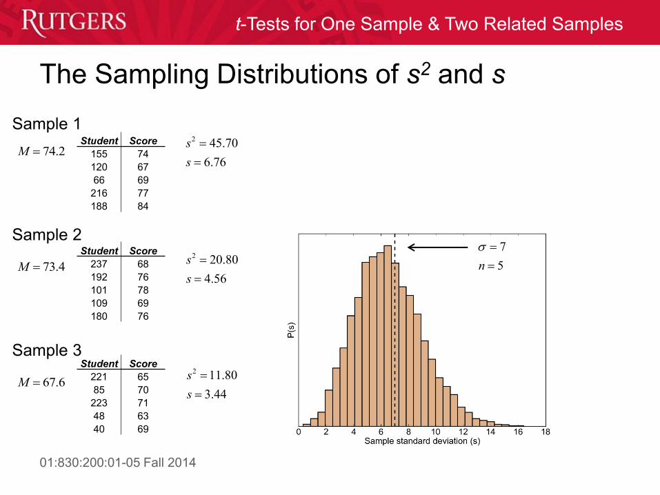
The Sampling Distributions of s2 and s
Student Score
155 74
120 67
66 69
216 77
188 84
Student Score
237 68
192 76
101 78
109 69
180 76
Student Score
221 65
85 70
223 71
48 63
40 69
Sample 1
Sample 2
Sample 3
74.2M
73.4M
67.6M
2 45.70
6.76
s
s
2 20.80
4.56
s
s
2 11.80
3.44
s
s
7
5n
01:830:200:01-05 Fall 2014
t-Tests for One Sample & Two Related Samples
The t-Statistic
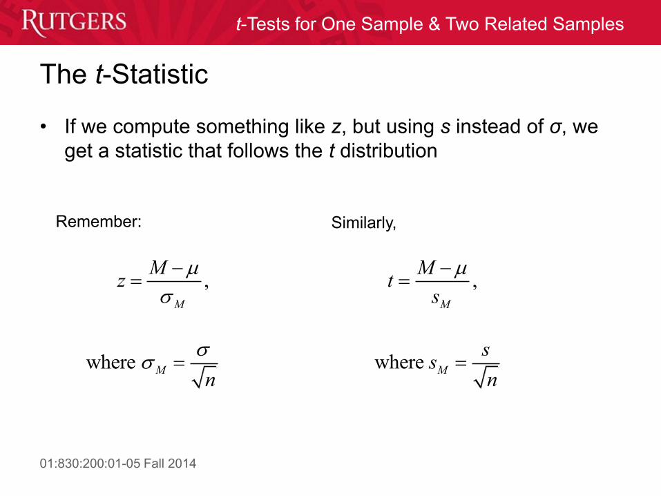
• If we compute something like z, but using s instead of σ, we
get a statistic that follows the t distribution
,M
zM
,
M
tM
s
Remember: Similarly,
where Mn
where Ms
n
s
01:830:200:01-05 Fall 2014
t-Tests for One Sample & Two Related Samples
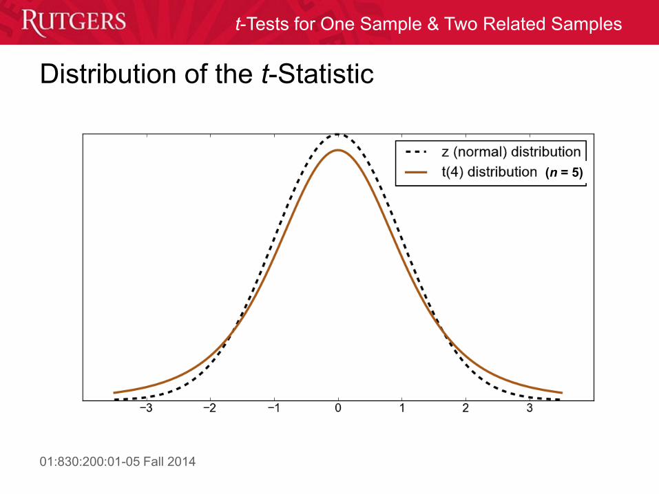
Distribution of the t-Statistic
(n = 5)
01:830:200:01-05 Fall 2014
t-Tests for One Sample & Two Related Samples
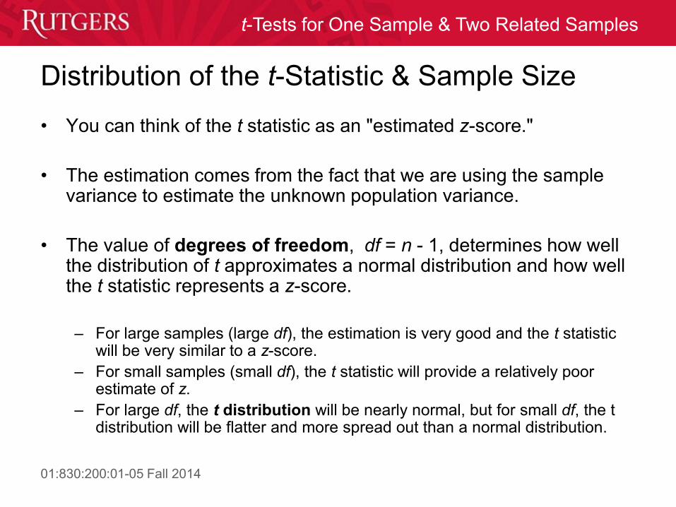
Distribution of the t-Statistic & Sample Size
• You can think of the t statistic as an "estimated z-score."
• The estimation comes from the fact that we are using the sample variance to estimate the unknown population variance.
• The value of degrees of freedom, df = n - 1, determines how well the distribution of t approximates a normal distribution and how well the t statistic represents a z-score.
– For large samples (large df), the estimation is very good and the t statistic
will be very similar to a z-score.
– For small samples (small df), the t statistic will provide a relatively poor estimate of z.
– For large df, the t distribution will be nearly normal, but for small df, the t distribution will be flatter and more spread out than a normal distribution.
01:830:200:01-05 Fall 2014
t-Tests for One Sample & Two Related Samples
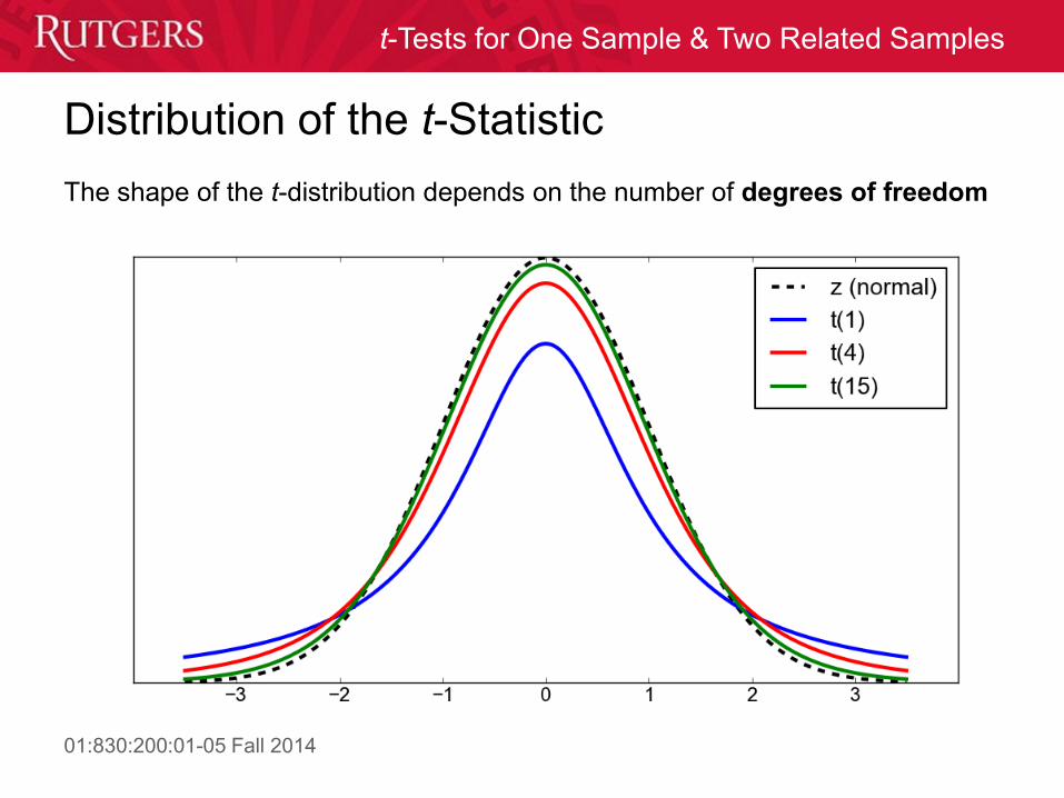
Distribution of the t-Statistic
The shape of the t-distribution depends on the number of degrees of freedom
01:830:200:01-05 Fall 2014
t-Tests for One Sample & Two Related Samples
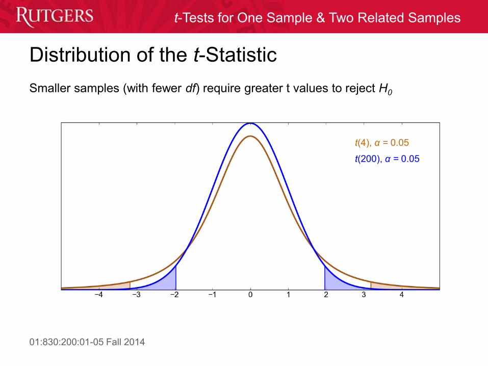
Distribution of the t-Statistic
Smaller samples (with fewer df) require greater t values to reject H0
t(4), α = 0.05
t(200), α = 0.05
01:830:200:01-05 Fall 2014
t-Tests for One Sample & Two Related Samples
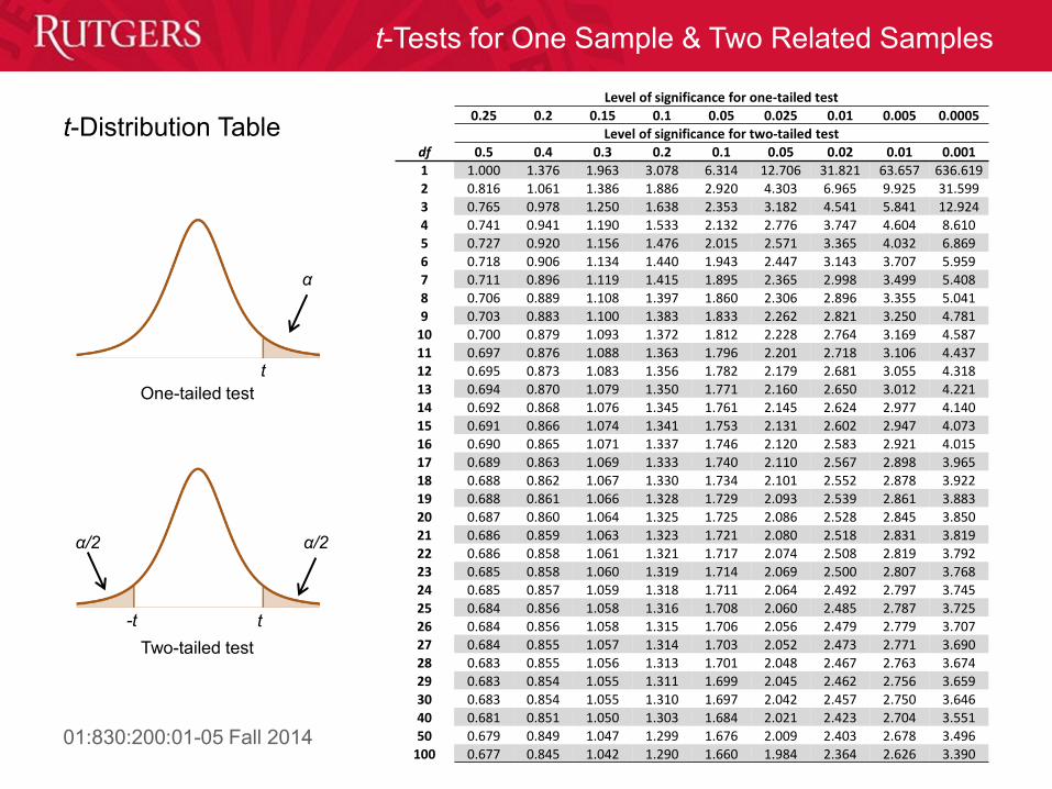
Level of significance for one-tailed test
0.25 0.2 0.15 0.1 0.05 0.025 0.01 0.005 0.0005
Level of significance for two-tailed test
df 0.5 0.4 0.3 0.2 0.1 0.05 0.02 0.01 0.001
1 1.000 1.376 1.963 3.078 6.314 12.706 31.821 63.657 636.619
2 0.816 1.061 1.386 1.886 2.920 4.303 6.965 9.925 31.599
3 0.765 0.978 1.250 1.638 2.353 3.182 4.541 5.841 12.924
4 0.741 0.941 1.190 1.533 2.132 2.776 3.747 4.604 8.610
5 0.727 0.920 1.156 1.476 2.015 2.571 3.365 4.032 6.869
6 0.718 0.906 1.134 1.440 1.943 2.447 3.143 3.707 5.959
7 0.711 0.896 1.119 1.415 1.895 2.365 2.998 3.499 5.408
8 0.706 0.889 1.108 1.397 1.860 2.306 2.896 3.355 5.041
9 0.703 0.883 1.100 1.383 1.833 2.262 2.821 3.250 4.781
10 0.700 0.879 1.093 1.372 1.812 2.228 2.764 3.169 4.587
11 0.697 0.876 1.088 1.363 1.796 2.201 2.718 3.106 4.437
12 0.695 0.873 1.083 1.356 1.782 2.179 2.681 3.055 4.318
13 0.694 0.870 1.079 1.350 1.771 2.160 2.650 3.012 4.221
14 0.692 0.868 1.076 1.345 1.761 2.145 2.624 2.977 4.140
15 0.691 0.866 1.074 1.341 1.753 2.131 2.602 2.947 4.073
16 0.690 0.865 1.071 1.337 1.746 2.120 2.583 2.921 4.015
17 0.689 0.863 1.069 1.333 1.740 2.110 2.567 2.898 3.965
18 0.688 0.862 1.067 1.330 1.734 2.101 2.552 2.878 3.922
19 0.688 0.861 1.066 1.328 1.729 2.093 2.539 2.861 3.883
20 0.687 0.860 1.064 1.325 1.725 2.086 2.528 2.845 3.850 21 0.686 0.859 1.063 1.323 1.721 2.080 2.518 2.831 3.819
22 0.686 0.858 1.061 1.321 1.717 2.074 2.508 2.819 3.792
23 0.685 0.858 1.060 1.319 1.714 2.069 2.500 2.807 3.768
24 0.685 0.857 1.059 1.318 1.711 2.064 2.492 2.797 3.745
25 0.684 0.856 1.058 1.316 1.708 2.060 2.485 2.787 3.725 26 0.684 0.856 1.058 1.315 1.706 2.056 2.479 2.779 3.707
27 0.684 0.855 1.057 1.314 1.703 2.052 2.473 2.771 3.690
28 0.683 0.855 1.056 1.313 1.701 2.048 2.467 2.763 3.674
29 0.683 0.854 1.055 1.311 1.699 2.045 2.462 2.756 3.659
30 0.683 0.854 1.055 1.310 1.697 2.042 2.457 2.750 3.646 40 0.681 0.851 1.050 1.303 1.684 2.021 2.423 2.704 3.551
50 0.679 0.849 1.047 1.299 1.676 2.009 2.403 2.678 3.496
100 0.677 0.845 1.042 1.290 1.660 1.984 2.364 2.626 3.390
t-Distribution Table
Two-tailed test
One-tailed test
α
t
α/2 α/2
t -t
01:830:200:01-05 Fall 2014
t-Tests for One Sample & Two Related Samples
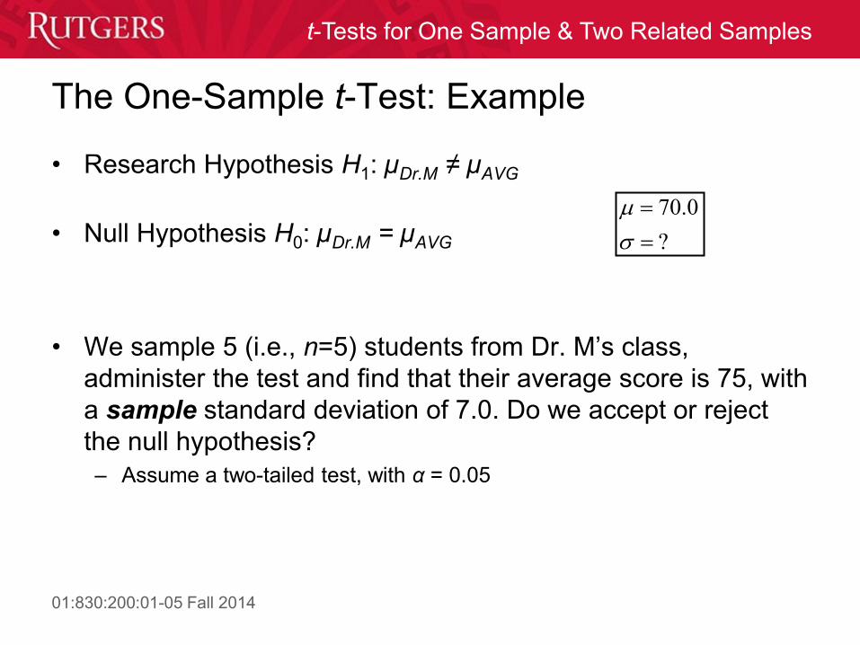
The One-Sample t-Test: Example
• Research Hypothesis H1: µDr.M ≠ µAVG
• Null Hypothesis H0: µDr.M = µAVG
• We sample 5 (i.e., n=5) students from Dr. M’s class,
administer the test and find that their average score is 75, with
a sample standard deviation of 7.0. Do we accept or reject
the null hypothesis?
– Assume a two-tailed test, with α = 0.05
70.0
?
01:830:200:01-05 Fall 2014
t-Tests for One Sample & Two Related Samples
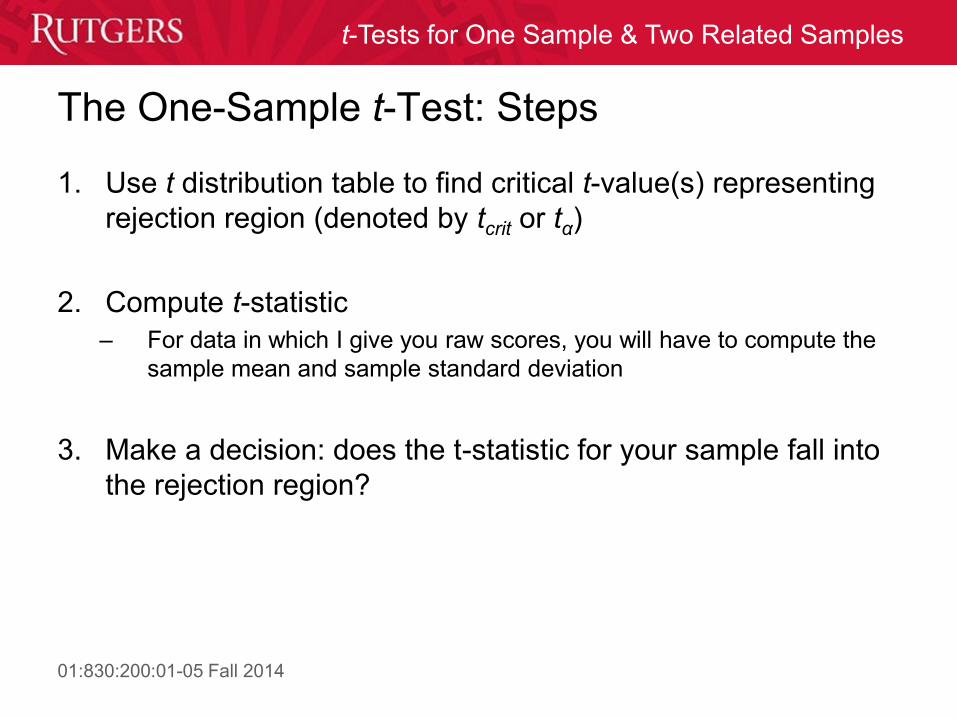
The One-Sample t-Test: Steps
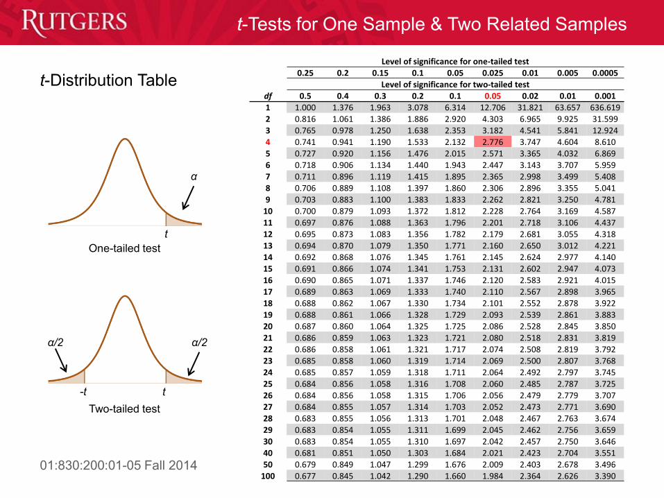
1. Use t distribution table to find critical t-value(s) representing
rejection region (denoted by tcrit or tα)
2. Compute t-statistic
– For data in which I give you raw scores, you will have to compute the
sample mean and sample standard deviation
3. Make a decision: does the t-statistic for your sample fall into
the rejection region?

01:830:200:01-05 Fall 2014
t-Tests for One Sample & Two Related Samples
Level of significance for one-tailed test
0.25 0.2 0.15 0.1 0.05 0.025 0.01 0.005 0.0005
Level of significance for two-tailed test
df 0.5 0.4 0.3 0.2 0.1 0.05 0.02 0.01 0.001
1 1.000 1.376 1.963 3.078 6.314 12.706 31.821 63.657 636.619
2 0.816 1.061 1.386 1.886 2.920 4.303 6.965 9.925 31.599
3 0.765 0.978 1.250 1.638 2.353 3.182 4.541 5.841 12.924
4 0.741 0.941 1.190 1.533 2.132 2.776 3.747 4.604 8.610
5 0.727 0.920 1.156 1.476 2.015 2.571 3.365 4.032 6.869
6 0.718 0.906 1.134 1.440 1.943 2.447 3.143 3.707 5.959
7 0.711 0.896 1.119 1.415 1.895 2.365 2.998 3.499 5.408
8 0.706 0.889 1.108 1.397 1.860 2.306 2.896 3.355 5.041
9 0.703 0.883 1.100 1.383 1.833 2.262 2.821 3.250 4.781
10 0.700 0.879 1.093 1.372 1.812 2.228 2.764 3.169 4.587
11 0.697 0.876 1.088 1.363 1.796 2.201 2.718 3.106 4.437
12 0.695 0.873 1.083 1.356 1.782 2.179 2.681 3.055 4.318
13 0.694 0.870 1.079 1.350 1.771 2.160 2.650 3.012 4.221
14 0.692 0.868 1.076 1.345 1.761 2.145 2.624 2.977 4.140
15 0.691 0.866 1.074 1.341 1.753 2.131 2.602 2.947 4.073
16 0.690 0.865 1.071 1.337 1.746 2.120 2.583 2.921 4.015
17 0.689 0.863 1.069 1.333 1.740 2.110 2.567 2.898 3.965
18 0.688 0.862 1.067 1.330 1.734 2.101 2.552 2.878 3.922
19 0.688 0.861 1.066 1.328 1.729 2.093 2.539 2.861 3.883
20 0.687 0.860 1.064 1.325 1.725 2.086 2.528 2.845 3.850 21 0.686 0.859 1.063 1.323 1.721 2.080 2.518 2.831 3.819
22 0.686 0.858 1.061 1.321 1.717 2.074 2.508 2.819 3.792
23 0.685 0.858 1.060 1.319 1.714 2.069 2.500 2.807 3.768
24 0.685 0.857 1.059 1.318 1.711 2.064 2.492 2.797 3.745
25 0.684 0.856 1.058 1.316 1.708 2.060 2.485 2.787 3.725 26 0.684 0.856 1.058 1.315 1.706 2.056 2.479 2.779 3.707
27 0.684 0.855 1.057 1.314 1.703 2.052 2.473 2.771 3.690
28 0.683 0.855 1.056 1.313 1.701 2.048 2.467 2.763 3.674
29 0.683 0.854 1.055 1.311 1.699 2.045 2.462 2.756 3.659
30 0.683 0.854 1.055 1.310 1.697 2.042 2.457 2.750 3.646 40 0.681 0.851 1.050 1.303 1.684 2.021 2.423 2.704 3.551
50 0.679 0.849 1.047 1.299 1.676 2.009 2.403 2.678 3.496
100 0.677 0.845 1.042 1.290 1.660 1.984 2.364 2.626 3.390
t-Distribution Table
Two-tailed test
One-tailed test
α
t
α/2 α/2
t -t
01:830:200:01-05 Fall 2014
t-Tests for One Sample & Two Related Samples
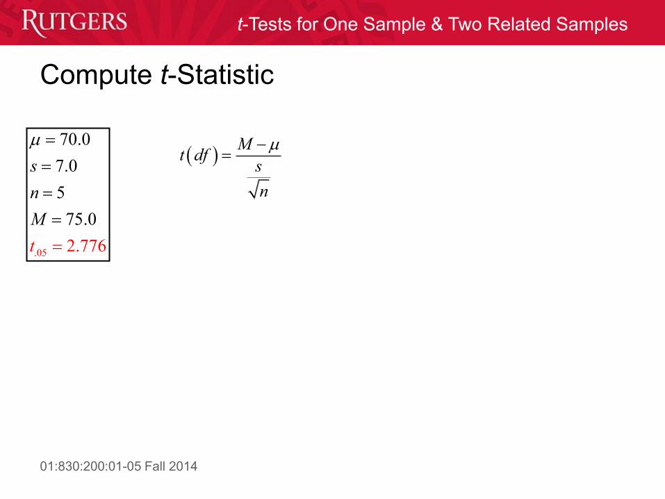
Compute t-Statistic
.05
70.0
7.0
2.776
5
75.0
s
n
M
t
M
dfs
t
n
01:830:200:01-05 Fall 2014
t-Tests for One Sample & Two Related Samples
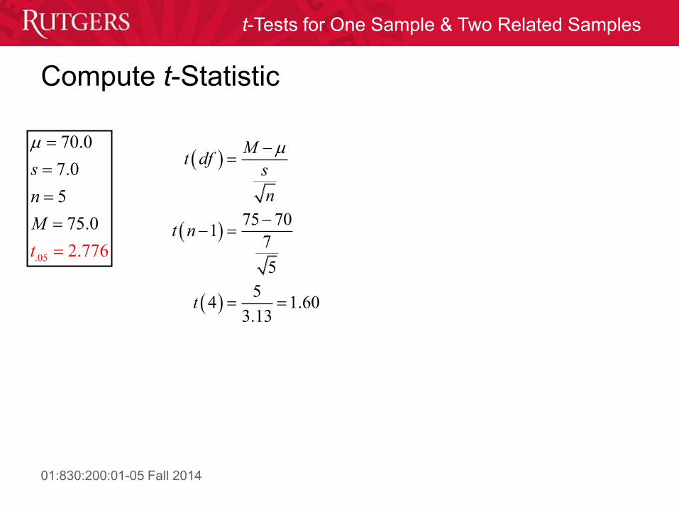
Compute t-Statistic
.05
70.0
7.0
2.776
5
75.0
s
n
M
t
75 701
7
5
54 1.60
3.13
Mdf
s
n
t n
t
t
01:830:200:01-05 Fall 2014
t-Tests for One Sample & Two Related Samples
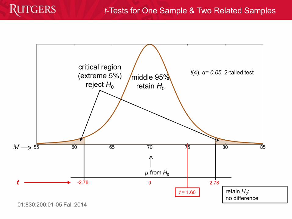
µ from H0
0 t
critical region
(extreme 5%)
reject H0 middle 95%
retain H0
t(4), α= 0.05, 2-tailed test
-2.78 2.78
M
t = 1.60 retain H0:
no difference
01:830:200:01-05 Fall 2014
t-Tests for One Sample & Two Related Samples
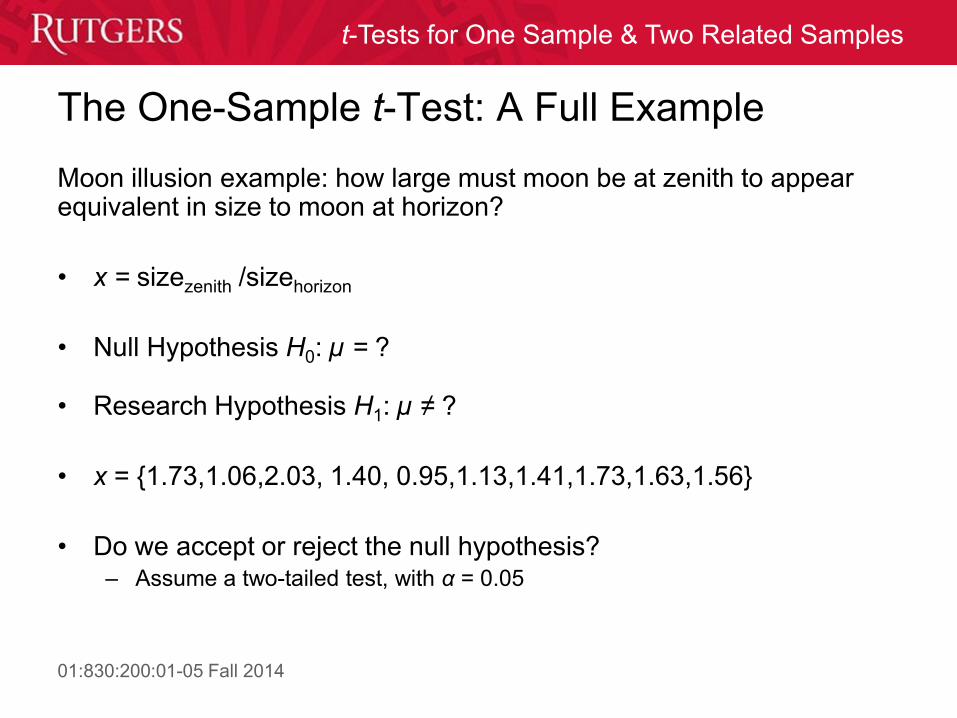
The One-Sample t-Test: A Full Example
Moon illusion example: how large must moon be at zenith to appear equivalent in size to moon at horizon?
• x = sizezenith /sizehorizon
• Null Hypothesis H0: µ = ?
• Research Hypothesis H1: µ ≠ ?
• x = {1.73,1.06,2.03, 1.40, 0.95,1.13,1.41,1.73,1.63,1.56}
• Do we accept or reject the null hypothesis? – Assume a two-tailed test, with α = 0.05

01:830:200:01-05 Fall 2014
t-Tests for One Sample & Two Related Samples
The One-Sample t-Test: A Full Example
Moon illusion example: how large must moon be at zenith to appear equivalent in size to moon at horizon?
• x = sizezenith /sizehorizon
• Null Hypothesis H0: µ = 1
• Research Hypothesis H1: µ ≠ 1
• x = {1.73,1.06,2.03, 1.40, 0.95,1.13,1.41,1.73,1.63,1.56}
• Do we accept or reject the null hypothesis? – Assume a two-tailed test, with α = 0.05

01:830:200:01-05 Fall 2014
t-Tests for One Sample & Two Related Samples
Level of significance for one-tailed test
0.25 0.2 0.15 0.1 0.05 0.025 0.01 0.005 0.0005
Level of significance for two-tailed test
df 0.5 0.4 0.3 0.2 0.1 0.05 0.02 0.01 0.001
1 1.000 1.376 1.963 3.078 6.314 12.706 31.821 63.657 636.619
2 0.816 1.061 1.386 1.886 2.920 4.303 6.965 9.925 31.599
3 0.765 0.978 1.250 1.638 2.353 3.182 4.541 5.841 12.924
4 0.741 0.941 1.190 1.533 2.132 2.776 3.747 4.604 8.610
5 0.727 0.920 1.156 1.476 2.015 2.571 3.365 4.032 6.869
6 0.718 0.906 1.134 1.440 1.943 2.447 3.143 3.707 5.959
7 0.711 0.896 1.119 1.415 1.895 2.365 2.998 3.499 5.408
8 0.706 0.889 1.108 1.397 1.860 2.306 2.896 3.355 5.041
9 0.703 0.883 1.100 1.383 1.833 2.262 2.821 3.250 4.781
10 0.700 0.879 1.093 1.372 1.812 2.228 2.764 3.169 4.587
11 0.697 0.876 1.088 1.363 1.796 2.201 2.718 3.106 4.437
12 0.695 0.873 1.083 1.356 1.782 2.179 2.681 3.055 4.318
13 0.694 0.870 1.079 1.350 1.771 2.160 2.650 3.012 4.221
14 0.692 0.868 1.076 1.345 1.761 2.145 2.624 2.977 4.140
15 0.691 0.866 1.074 1.341 1.753 2.131 2.602 2.947 4.073
16 0.690 0.865 1.071 1.337 1.746 2.120 2.583 2.921 4.015
17 0.689 0.863 1.069 1.333 1.740 2.110 2.567 2.898 3.965
18 0.688 0.862 1.067 1.330 1.734 2.101 2.552 2.878 3.922
19 0.688 0.861 1.066 1.328 1.729 2.093 2.539 2.861 3.883
20 0.687 0.860 1.064 1.325 1.725 2.086 2.528 2.845 3.850 21 0.686 0.859 1.063 1.323 1.721 2.080 2.518 2.831 3.819
22 0.686 0.858 1.061 1.321 1.717 2.074 2.508 2.819 3.792
23 0.685 0.858 1.060 1.319 1.714 2.069 2.500 2.807 3.768
24 0.685 0.857 1.059 1.318 1.711 2.064 2.492 2.797 3.745
25 0.684 0.856 1.058 1.316 1.708 2.060 2.485 2.787 3.725 26 0.684 0.856 1.058 1.315 1.706 2.056 2.479 2.779 3.707
27 0.684 0.855 1.057 1.314 1.703 2.052 2.473 2.771 3.690
28 0.683 0.855 1.056 1.313 1.701 2.048 2.467 2.763 3.674
29 0.683 0.854 1.055 1.311 1.699 2.045 2.462 2.756 3.659
30 0.683 0.854 1.055 1.310 1.697 2.042 2.457 2.750 3.646 40 0.681 0.851 1.050 1.303 1.684 2.021 2.423 2.704 3.551
50 0.679 0.849 1.047 1.299 1.676 2.009 2.403 2.678 3.496
100 0.677 0.845 1.042 1.290 1.660 1.984 2.364 2.626 3.390
t-Distribution Table
Two-tailed test
One-tailed test
α
t
α/2 α/2
t -t
01:830:200:01-05 Fall 2014
t-Tests for One Sample & Two Related Samples
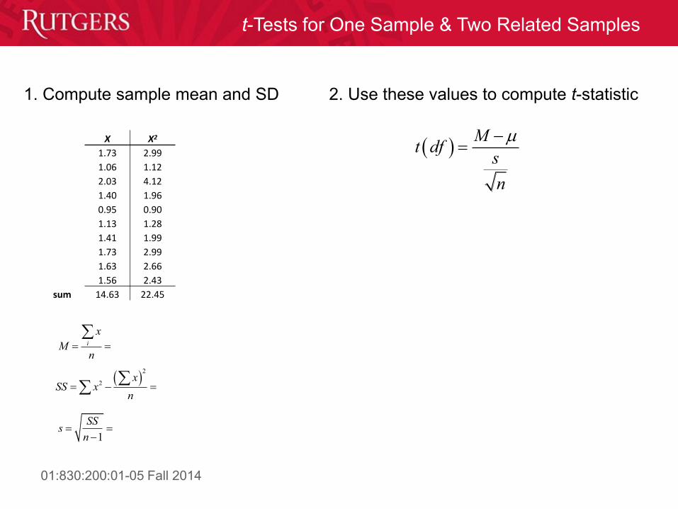
X X2
1.73 2.99
1.06 1.12
2.03 4.12
1.40 1.96
0.95 0.90
1.13 1.28
1.41 1.99
1.73 2.99
1.63 2.66
1.56 2.43
sum 14.63 22.45
i
x
Mn
2
2x
S xn
S
1s
SS
n
1. Compute sample mean and SD 2. Use these values to compute t-statistic
M
dfs
t
n
01:830:200:01-05 Fall 2014
t-Tests for One Sample & Two Related Samples
X X2
1.73 2.99
1.06 1.12
2.03 4.12
1.40 1.96
0.95 0.90
1.13 1.28
1.41 1.99
1.73 2.99
1.63 2.66
1.56 2.43
sum 14.63 22.45
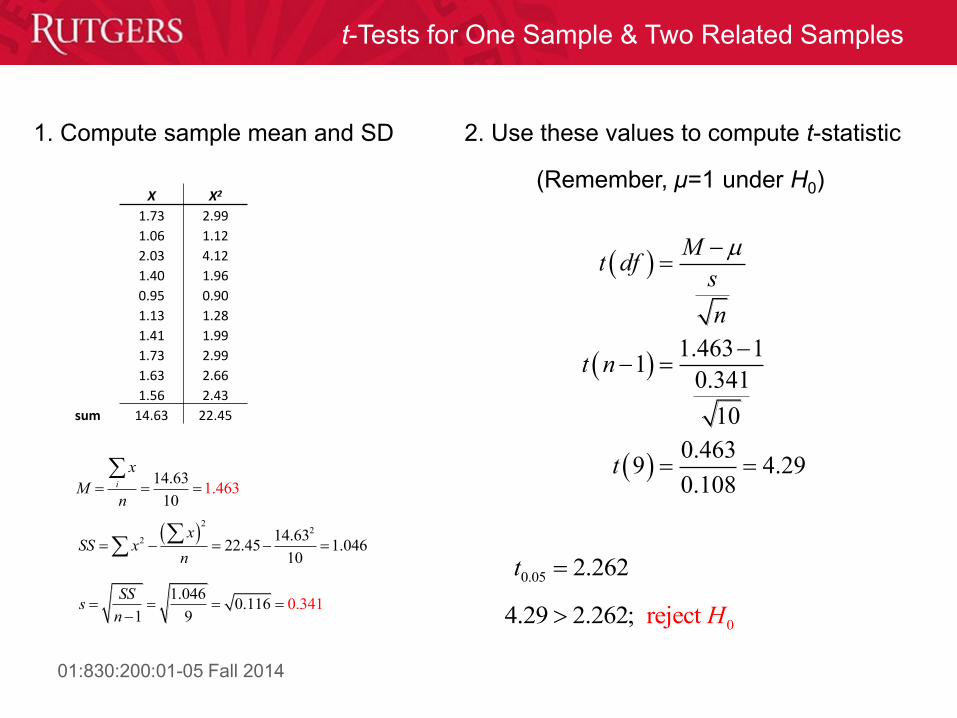
14.63
101.463i
x
Mn
2
22 14.63
22.45 1.04610
xxSS
n
1.046
1 90.116 0.341
SS
ns
1. Compute sample mean and SD 2. Use these values to compute t-statistic
1.463 11
0.341
10
0.4639 4.29
0.108
Mdf
s
t n
t
t
n
(Remember, µ=1 under H0)
0.05 2.262t
04.29 2.262; reject H
01:830:200:01-05 Fall 2014
t-Tests for One Sample & Two Related Samples
Hypothesis Testing with the t-Statistic
• Both the sample size and the sample variance influence the
outcome of a hypothesis test.
• The sample size is inversely related to the estimated standard
error. Therefore, a large sample size increases the likelihood
of a significant test (for an existing effect).
• The sample variance, on the other hand, is directly related to
the estimated standard error. Therefore, a large variance
decreases the likelihood of a significant test (for an existing
effect).
01:830:200:01-05 Fall 2014
t-Tests for One Sample & Two Related Samples
• The related-samples t-test allows researchers to evaluate the
mean difference between two treatment conditions using the
data from a single sample.
– This test can also be called the repeated-measures t-test, the matched-
samples t-test, or the paired-samples t-test
• In a repeated-measures design, a single group of individuals
is obtained and each individual is measured in both of the
treatment conditions being compared.
• Thus, the data consist of two scores for each individual.
t-Tests for Two Related Samples: Repeated Measures
01:830:200:01-05 Fall 2014
t-Tests for One Sample & Two Related Samples
t-Tests for Two Related Samples: Matched Subjects
• The related-samples t test can also be used for a similar
design, called a matched-subjects design, in which each
individual in one treatment is matched one-to-one with a
corresponding individual in the second treatment.
• The matching is accomplished by selecting pairs of subjects
so that the two subjects in each pair have identical (or nearly
identical) scores on the variable that is being used for
matching.
01:830:200:01-05 Fall 2014
t-Tests for One Sample & Two Related Samples
t-Statistic for Two Related Samples
• The repeated-measures t statistic allows researchers to test a
hypothesis about the population mean difference between two
treatment conditions using sample data from a repeated-
measures research study.
• In this situation it is possible to compute a difference score for
each individual:
difference score = D = x2 – x1
where x1 is the person’s score in the first treatment and x2 is the
score in the second treatment.
01:830:200:01-05 Fall 2014
t-Tests for One Sample & Two Related Samples
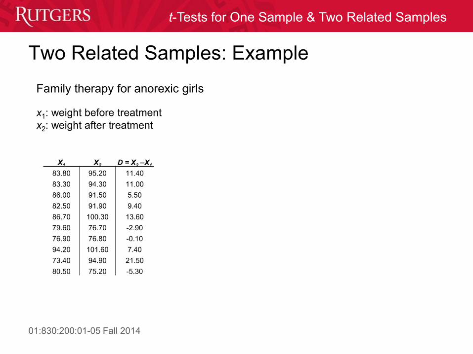
Two Related Samples: Example
X1 X2 D = X2 –X1
83.80 95.20 11.40
83.30 94.30 11.00
86.00 91.50 5.50
82.50 91.90 9.40
86.70 100.30 13.60
79.60 76.70 -2.90
76.90 76.80 -0.10
94.20 101.60 7.40
73.40 94.90 21.50
80.50 75.20 -5.30
x1: weight before treatment
x2: weight after treatment
Family therapy for anorexic girls
01:830:200:01-05 Fall 2014
t-Tests for One Sample & Two Related Samples
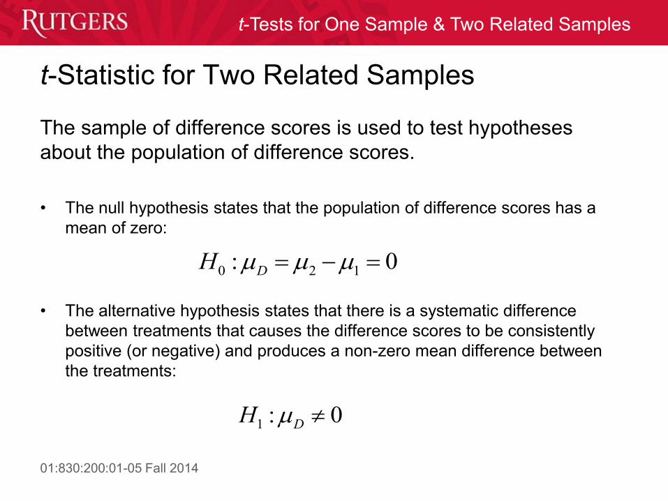
t-Statistic for Two Related Samples
The sample of difference scores is used to test hypotheses
about the population of difference scores.
• The null hypothesis states that the population of difference scores has a
mean of zero:
• The alternative hypothesis states that there is a systematic difference
between treatments that causes the difference scores to be consistently
positive (or negative) and produces a non-zero mean difference between
the treatments:
0 2 1: 0DH
1 : 0DH
01:830:200:01-05 Fall 2014
t-Tests for One Sample & Two Related Samples
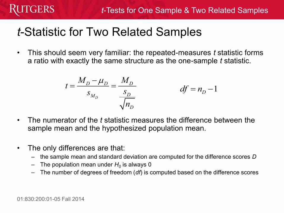
• This should seem very familiar: the repeated-measures t statistic forms a ratio with exactly the same structure as the one-sample t statistic.
• The numerator of the t statistic measures the difference between the sample mean and the hypothesized population mean.
• The only differences are that: – the sample mean and standard deviation are computed for the difference scores D
– The population mean under H0 is always 0
– The number of degrees of freedom (df) is computed based on the difference scores
t-Statistic for Two Related Samples
D
D D D
DM
D
M M
s s
n
t
1Ddf n
01:830:200:01-05 Fall 2014
t-Tests for One Sample & Two Related Samples
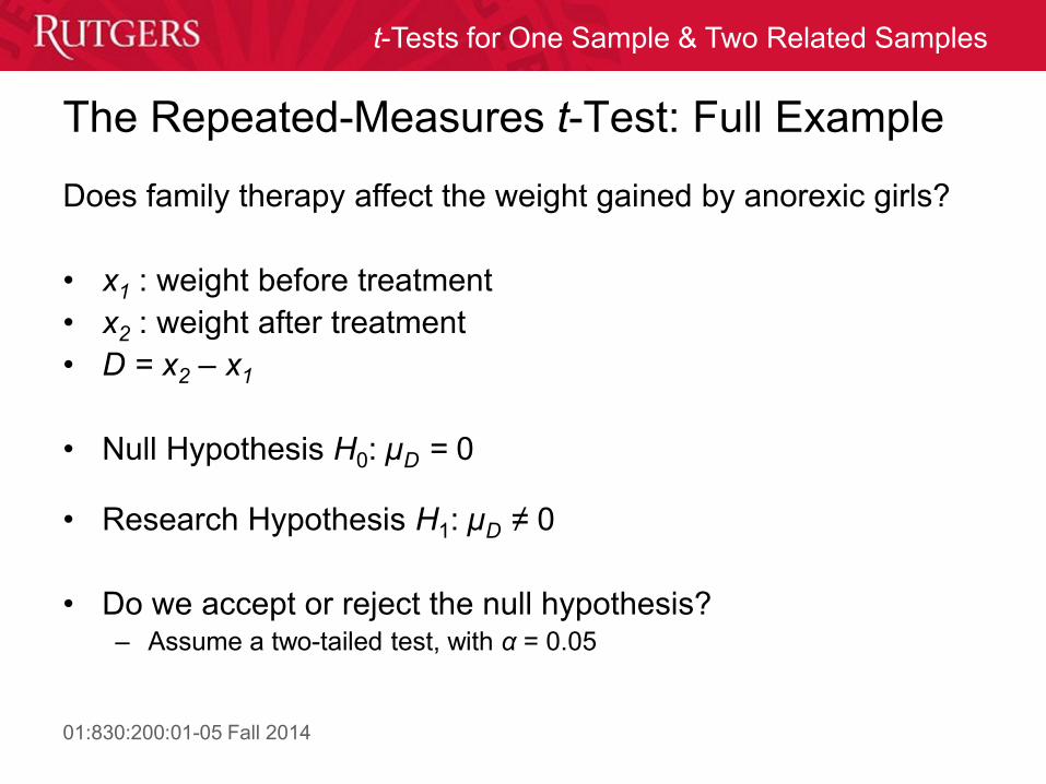
The Repeated-Measures t-Test: Full Example
Does family therapy affect the weight gained by anorexic girls?
• x1 : weight before treatment
• x2 : weight after treatment
• D = x2 – x1
• Null Hypothesis H0: µD = 0
• Research Hypothesis H1: µD ≠ 0
• Do we accept or reject the null hypothesis? – Assume a two-tailed test, with α = 0.05
01:830:200:01-05 Fall 2014
t-Tests for One Sample & Two Related Samples
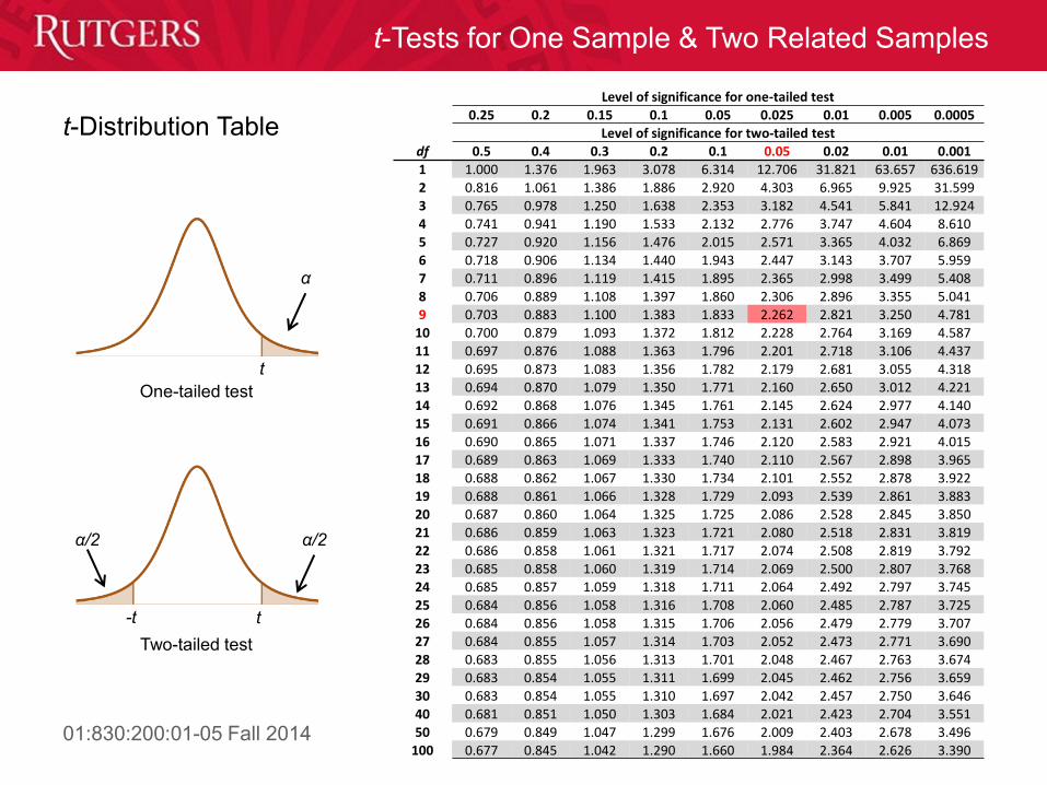
Level of significance for one-tailed test
0.25 0.2 0.15 0.1 0.05 0.025 0.01 0.005 0.0005
Level of significance for two-tailed test
df 0.5 0.4 0.3 0.2 0.1 0.05 0.02 0.01 0.001
1 1.000 1.376 1.963 3.078 6.314 12.706 31.821 63.657 636.619
2 0.816 1.061 1.386 1.886 2.920 4.303 6.965 9.925 31.599
3 0.765 0.978 1.250 1.638 2.353 3.182 4.541 5.841 12.924
4 0.741 0.941 1.190 1.533 2.132 2.776 3.747 4.604 8.610
5 0.727 0.920 1.156 1.476 2.015 2.571 3.365 4.032 6.869
6 0.718 0.906 1.134 1.440 1.943 2.447 3.143 3.707 5.959
7 0.711 0.896 1.119 1.415 1.895 2.365 2.998 3.499 5.408
8 0.706 0.889 1.108 1.397 1.860 2.306 2.896 3.355 5.041
9 0.703 0.883 1.100 1.383 1.833 2.262 2.821 3.250 4.781
10 0.700 0.879 1.093 1.372 1.812 2.228 2.764 3.169 4.587
11 0.697 0.876 1.088 1.363 1.796 2.201 2.718 3.106 4.437
12 0.695 0.873 1.083 1.356 1.782 2.179 2.681 3.055 4.318
13 0.694 0.870 1.079 1.350 1.771 2.160 2.650 3.012 4.221
14 0.692 0.868 1.076 1.345 1.761 2.145 2.624 2.977 4.140
15 0.691 0.866 1.074 1.341 1.753 2.131 2.602 2.947 4.073
16 0.690 0.865 1.071 1.337 1.746 2.120 2.583 2.921 4.015
17 0.689 0.863 1.069 1.333 1.740 2.110 2.567 2.898 3.965
18 0.688 0.862 1.067 1.330 1.734 2.101 2.552 2.878 3.922
19 0.688 0.861 1.066 1.328 1.729 2.093 2.539 2.861 3.883
20 0.687 0.860 1.064 1.325 1.725 2.086 2.528 2.845 3.850 21 0.686 0.859 1.063 1.323 1.721 2.080 2.518 2.831 3.819
22 0.686 0.858 1.061 1.321 1.717 2.074 2.508 2.819 3.792
23 0.685 0.858 1.060 1.319 1.714 2.069 2.500 2.807 3.768
24 0.685 0.857 1.059 1.318 1.711 2.064 2.492 2.797 3.745
25 0.684 0.856 1.058 1.316 1.708 2.060 2.485 2.787 3.725 26 0.684 0.856 1.058 1.315 1.706 2.056 2.479 2.779 3.707
27 0.684 0.855 1.057 1.314 1.703 2.052 2.473 2.771 3.690
28 0.683 0.855 1.056 1.313 1.701 2.048 2.467 2.763 3.674
29 0.683 0.854 1.055 1.311 1.699 2.045 2.462 2.756 3.659
30 0.683 0.854 1.055 1.310 1.697 2.042 2.457 2.750 3.646 40 0.681 0.851 1.050 1.303 1.684 2.021 2.423 2.704 3.551
50 0.679 0.849 1.047 1.299 1.676 2.009 2.403 2.678 3.496
100 0.677 0.845 1.042 1.290 1.660 1.984 2.364 2.626 3.390
t-Distribution Table
Two-tailed test
One-tailed test
α
t
α/2 α/2
t -t
01:830:200:01-05 Fall 2014
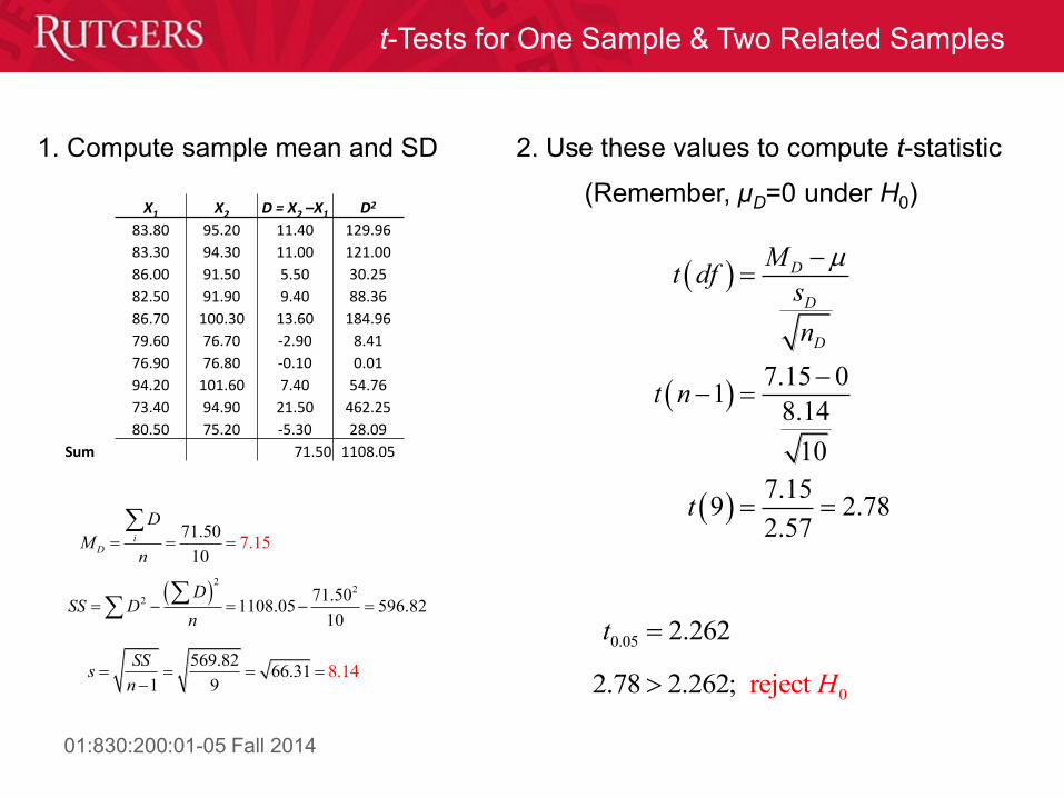
t-Tests for One Sample & Two Related Samples
71.50
17.15
0
iD
D
Mn
2
22 71.50
1108.05 596.8210
DSS D
n
569.826
16 8.1. 1
93 4
SS
ns
1. Compute sample mean and SD 2. Use these values to compute t-statistic
7.15 01
8.14
10
7.159 2.78
2.57
D
D
D
Mdf
n
n
t
ts
t
(Remember, µD=0 under H0) X1 X2 D = X2 –X1 D2
83.80 95.20 11.40 129.96
83.30 94.30 11.00 121.00
86.00 91.50 5.50 30.25
82.50 91.90 9.40 88.36
86.70 100.30 13.60 184.96
79.60 76.70 -2.90 8.41
76.90 76.80 -0.10 0.01
94.20 101.60 7.40 54.76
73.40 94.90 21.50 462.25
80.50 75.20 -5.30 28.09
Sum 71.50 1108.05
02.78 2.262; reject H
0.05 2.262t
01:830:200:01-05 Fall 2014
t-Tests for One Sample & Two Related Samples
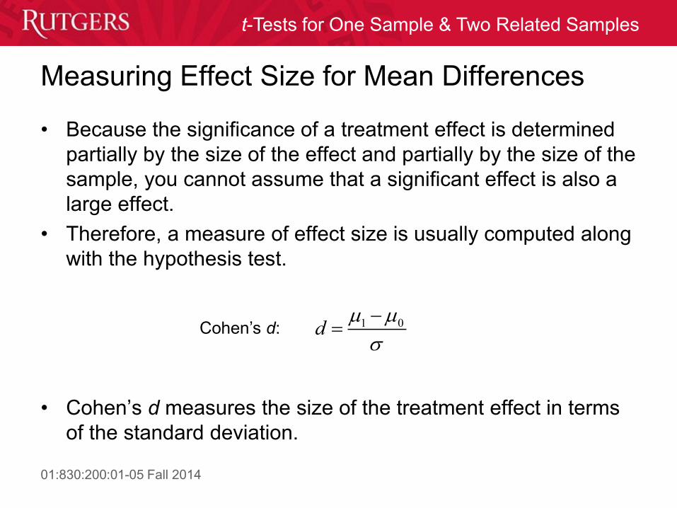
Measuring Effect Size for Mean Differences
• Because the significance of a treatment effect is determined
partially by the size of the effect and partially by the size of the
sample, you cannot assume that a significant effect is also a
large effect.
• Therefore, a measure of effect size is usually computed along
with the hypothesis test.
• Cohen’s d measures the size of the treatment effect in terms
of the standard deviation.
1 0d
Cohen’s d:
01:830:200:01-05 Fall 2014
t-Tests for One Sample & Two Related Samples
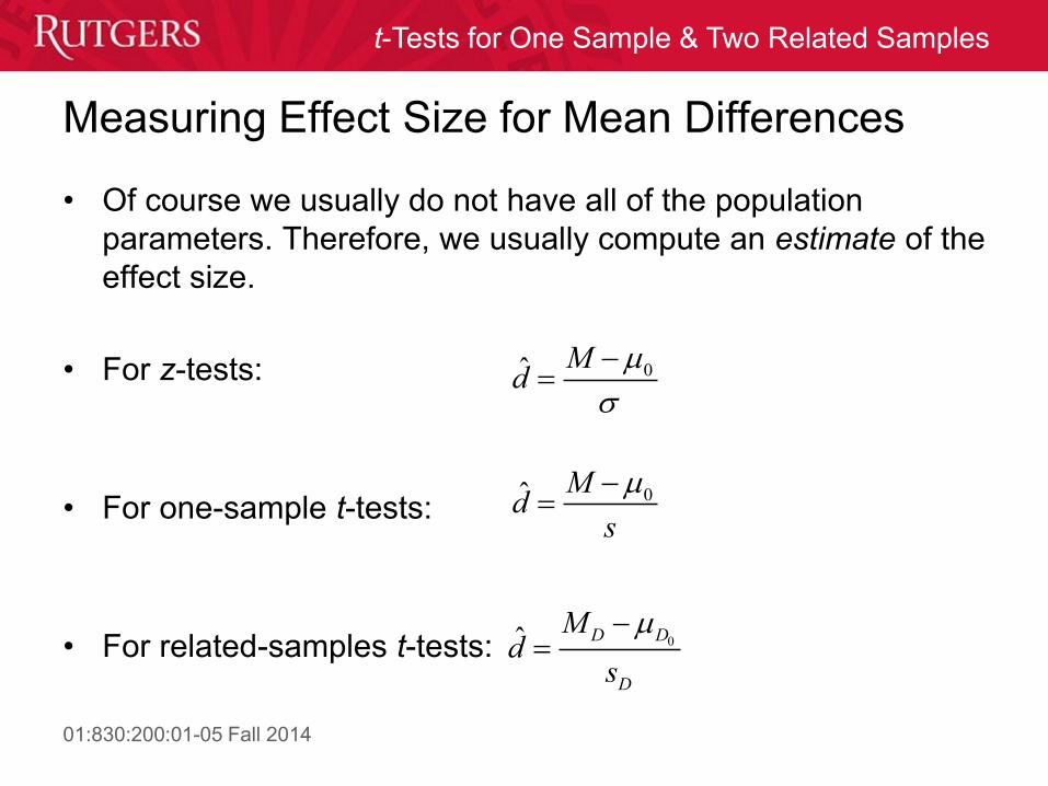
Measuring Effect Size for Mean Differences
• Of course we usually do not have all of the population
parameters. Therefore, we usually compute an estimate of the
effect size.
• For z-tests:
• For one-sample t-tests:
• For related-samples t-tests:
0ˆ Md
0d̂s
M
0ˆ D D
D
M
sd
01:830:200:01-05 Fall 2014
t-Tests for One Sample & Two Related Samples
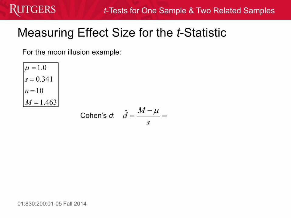
Measuring Effect Size for the t-Statistic
ˆ Md
s
Cohen’s d:
For the moon illusion example:
1.0
0.341
10
1.463
s
n
M
01:830:200:01-05 Fall 2014
t-Tests for One Sample & Two Related Samples
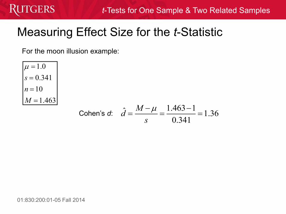
Measuring Effect Size for the t-Statistic
1.463 1ˆ 1.360.341
Md
s
Cohen’s d:
For the moon illusion example:
1.0
0.341
10
1.463
s
n
M