Advanced Process ControlTutorial Problem Set 2

Development of Control Relevant Models through System Identification

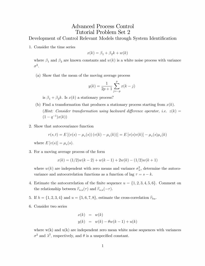
1. Consider the time series

x(k) = β1 + β2k + w(k)

where β1 and β2 are known constants and w(k) is a white noise process with variance

σ2.

(a) Show that the mean of the moving average process

y(k) =1

2p+ 1

p∑j=−p

x(k − j)

is β1 + β2k. Is x(k) a stationary process?

(b) Find a transformation that produces a stationary process starting from x(k).

(Hint: Consider transformation using backward difference operator, i.e. z(k) =

(1− q−1)x(k))

2. Show that autocovariance function

r(s, t) = E [(v(s)− µv(s)) (v(k)− µv(k))] = E [v(s)v(k)]− µv(s)µv(k)

where E [v(s)] = µv(s).

3. For a moving average process of the form

x(k) = (1/2)w(k − 2) + w(k − 1) + 2w(k)− (1/2)w(k + 1)

where w(k) are independent with zero means and variance σ2w, determine the autoco-

variance and autocorrelation functions as a function of lag τ = s− k.

4. Estimate the autocorrelation of the finite sequence u = 1, 2, 3, 4, 5, 6. Comment onthe relationship between ru,u(τ) and ru,u(−τ).

5. If h = 1, 2, 3, 4 and u = 5, 6, 7, 8, estimate the cross-correlation rhu.

6. Consider two series

x(k) = w(k)

y(k) = w(k)− θw(k − 1) + u(k)

where w(k) and u(k) are independent zero mean white noise sequences with variances

σ2 and λ2, respectively, and θ is a unspecified constant.

1

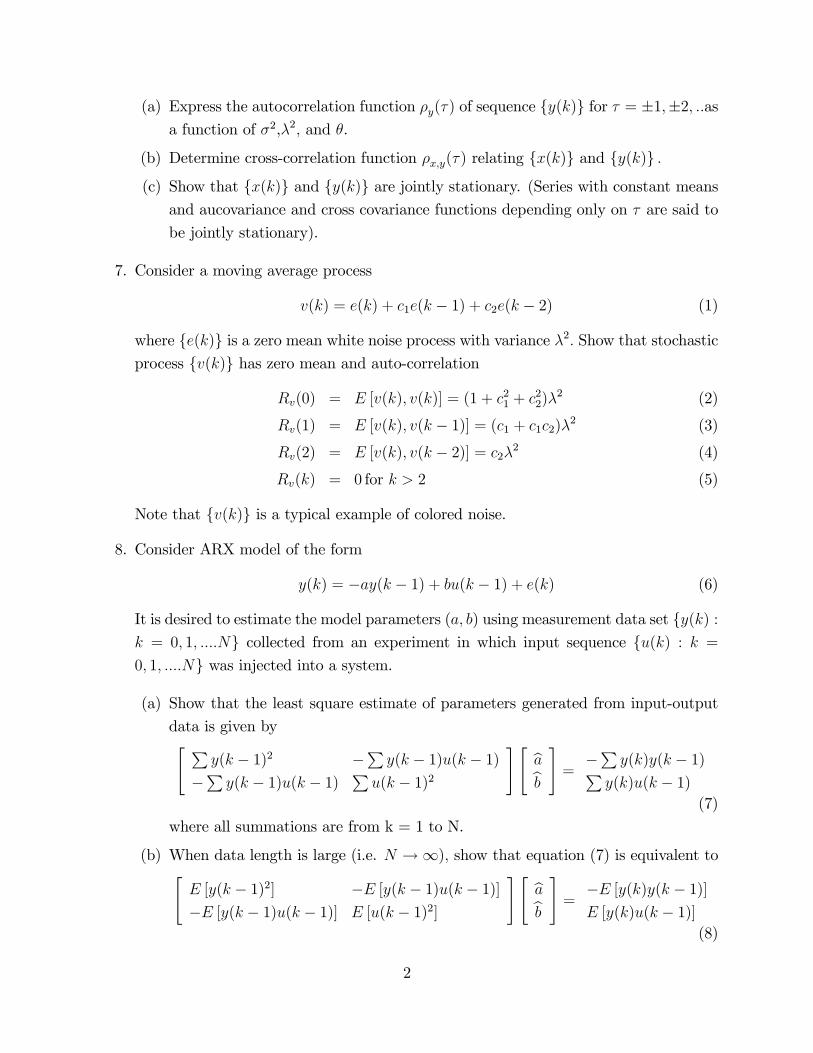
(a) Express the autocorrelation function ρy(τ) of sequence y(k) for τ = ±1,±2, ..as

a function of σ2,λ2, and θ.

(b) Determine cross-correlation function ρx,y(τ) relating x(k) and y(k) .

(c) Show that x(k) and y(k) are jointly stationary. (Series with constant meansand aucovariance and cross covariance functions depending only on τ are said to

be jointly stationary).

7. Consider a moving average process

v(k) = e(k) + c1e(k − 1) + c2e(k − 2) (1)

where e(k) is a zero mean white noise process with variance λ2. Show that stochasticprocess v(k) has zero mean and auto-correlation

Rv(0) = E [v(k), v(k)] = (1 + c21 + c22)λ2 (2)

Rv(1) = E [v(k), v(k − 1)] = (c1 + c1c2)λ2 (3)

Rv(2) = E [v(k), v(k − 2)] = c2λ2 (4)

Rv(k) = 0 for k > 2 (5)

Note that v(k) is a typical example of colored noise.

8. Consider ARX model of the form

y(k) = −ay(k − 1) + bu(k − 1) + e(k) (6)

It is desired to estimate the model parameters (a, b) using measurement data set y(k) :

k = 0, 1, ....N collected from an experiment in which input sequence u(k) : k =

0, 1, ....N was injected into a system.

(a) Show that the least square estimate of parameters generated from input-output

data is given by[ ∑y(k − 1)2 −

∑y(k − 1)u(k − 1)

−∑y(k − 1)u(k − 1)

∑u(k − 1)2

][a

b

]=−∑y(k)y(k − 1)∑

y(k)u(k − 1)

(7)

where all summations are from k = 1 to N.

(b) When data length is large (i.e. N →∞), show that equation (7) is equivalent to[E [y(k − 1)2] −E [y(k − 1)u(k − 1)]

−E [y(k − 1)u(k − 1)] E [u(k − 1)2]

][a

b

]=−E [y(k)y(k − 1)]

E [y(k)u(k − 1)]

(8)

2

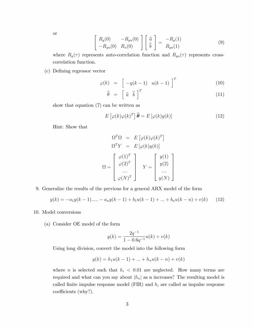
or [Ry(0) −Ryu(0)

−Ryu(0) Ru(0)

][a

b

]=−Ry(1)

Ryu(1)(9)

where Ry(τ) represents auto-correlation function and Ryu(τ) represents cross-

correlation function.

(c) Defining regressor vector

ϕ(k) =[−y(k − 1) u(k − 1)

]T(10)

θ =[a b

]T(11)

show that equation (7) can be written as

E[ϕ(k)ϕ(k)T

]θ = E [ϕ(k)y(k)] (12)

Hint: Show that

ΩTΩ = E[ϕ(k)ϕ(k)T

]ΩTY = E [ϕ(k)y(k)]

Ω =

ϕ(1)T

ϕ(2)T

....

ϕ(N)T

Y =

y(1)

y(2)

....

y(N)

9. Generalize the results of the previous for a general ARX model of the form

y(k) = −a1y(k − 1).....− any(k − 1) + b1u(k − 1) + ...+ bnu(k − n) + e(k) (13)

10. Model conversions

(a) Consider OE model of the form

y(k) =2q−1

1− 0.6q−1u(k) + v(k)

Using long division, convert the model into the following form

y(k) = h1u(k − 1) + ...+ hnu(k − n) + v(k)

where n is selected such that hi < 0.01 are neglected. How many terms are

required and what can you say about |hn| as n increases? The resulting model iscalled finite impulse response model (FIR) and hi are called as impulse response

coeffi cients (why?).

3

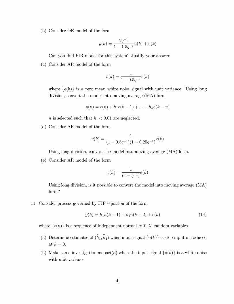
(b) Consider OE model of the form

y(k) =2q−1

1− 1.5q−1u(k) + v(k)

Can you find FIR model for this system? Justify your answer.

(c) Consider AR model of the form

v(k) =1

1− 0.5q−1e(k)

where e(k) is a zero mean white noise signal with unit variance. Using long

division, convert the model into moving average (MA) form

y(k) = e(k) + h1e(k − 1) + ...+ hne(k − n)

n is selected such that hi < 0.01 are neglected.

(d) Consider AR model of the form

v(k) =1

(1− 0.5q−1)(1− 0.25q−1)e(k)

Using long division, convert the model into moving average (MA) form.

(e) Consider AR model of the form

v(k) =1

(1− q−1)e(k)

Using long division, is it possible to convert the model into moving average (MA)

form?

11. Consider process governed by FIR equation of the form

y(k) = h1u(k − 1) + h2u(k − 2) + e(k) (14)

where e(k) is a sequence of independent normal N(0, λ) random variables.

(a) Determine estimates of (h1, h2) when input signal u(k) is step input introducedat k = 0.

(b) Make same investigation as part(a) when the input signal u(k) is a white noisewith unit variance.

4

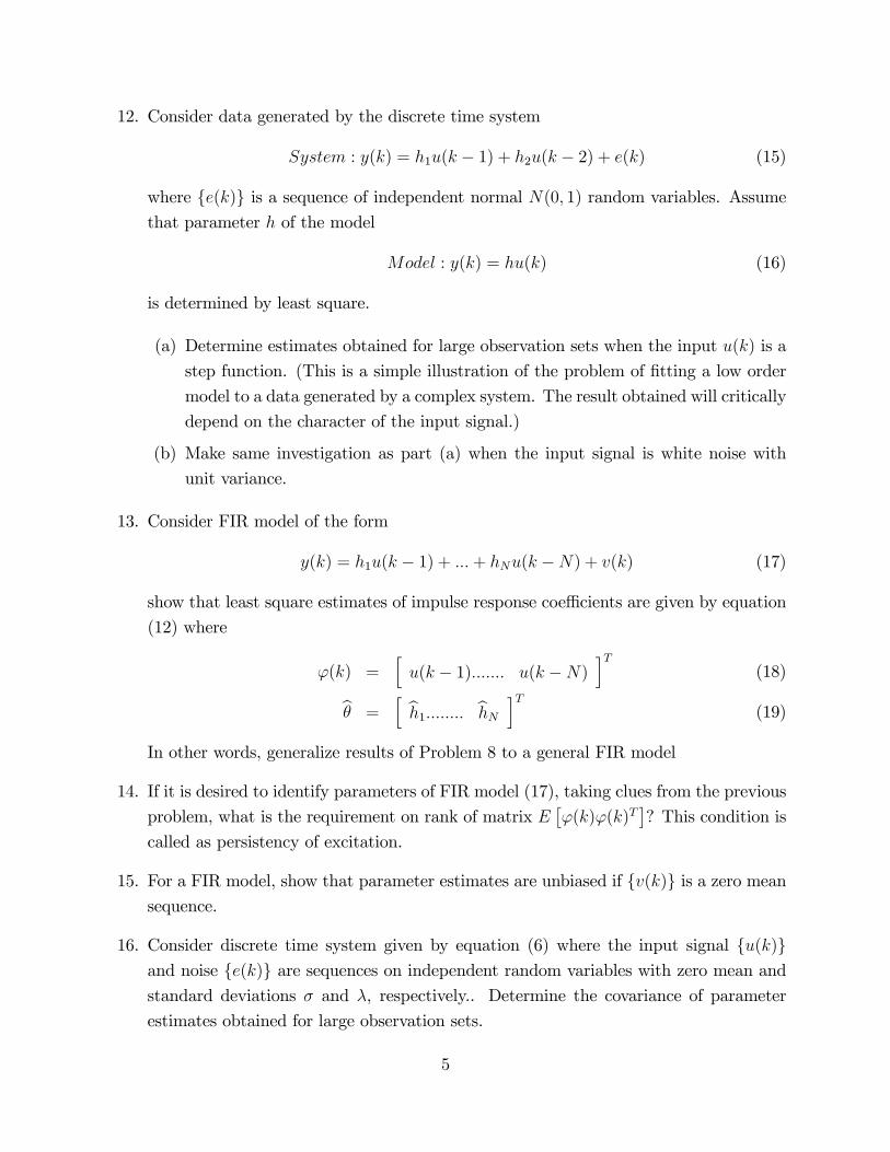
12. Consider data generated by the discrete time system

System : y(k) = h1u(k − 1) + h2u(k − 2) + e(k) (15)

where e(k) is a sequence of independent normal N(0, 1) random variables. Assume

that parameter h of the model

Model : y(k) = hu(k) (16)

is determined by least square.

(a) Determine estimates obtained for large observation sets when the input u(k) is a

step function. (This is a simple illustration of the problem of fitting a low order

model to a data generated by a complex system. The result obtained will critically

depend on the character of the input signal.)

(b) Make same investigation as part (a) when the input signal is white noise with

unit variance.

13. Consider FIR model of the form

y(k) = h1u(k − 1) + ...+ hNu(k −N) + v(k) (17)

show that least square estimates of impulse response coeffi cients are given by equation

(12) where

ϕ(k) =[u(k − 1)....... u(k −N)

]T(18)

θ =[h1........ hN

]T(19)

In other words, generalize results of Problem 8 to a general FIR model

14. If it is desired to identify parameters of FIR model (17), taking clues from the previous

problem, what is the requirement on rank of matrix E[ϕ(k)ϕ(k)T

]? This condition is

called as persistency of excitation.

15. For a FIR model, show that parameter estimates are unbiased if v(k) is a zero meansequence.

16. Consider discrete time system given by equation (6) where the input signal u(k)and noise e(k) are sequences on independent random variables with zero mean and

standard deviations σ and λ, respectively.. Determine the covariance of parameter

estimates obtained for large observation sets.

5

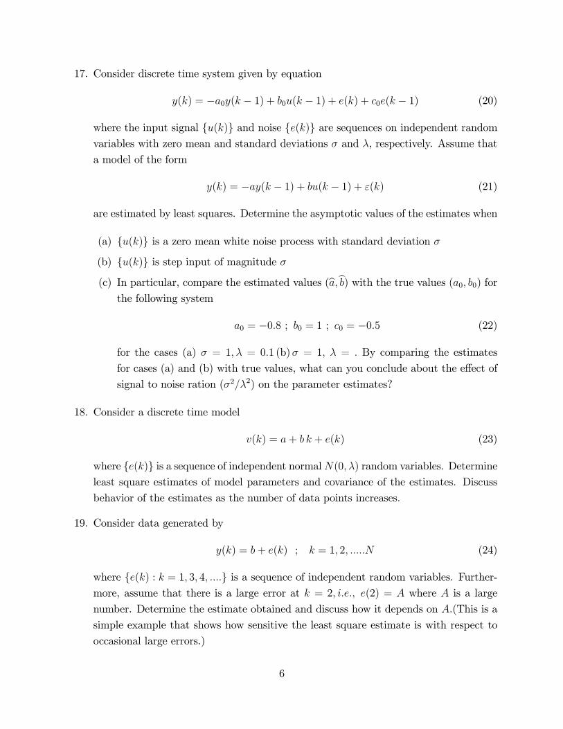
17. Consider discrete time system given by equation

y(k) = −a0y(k − 1) + b0u(k − 1) + e(k) + c0e(k − 1) (20)

where the input signal u(k) and noise e(k) are sequences on independent randomvariables with zero mean and standard deviations σ and λ, respectively. Assume that

a model of the form

y(k) = −ay(k − 1) + bu(k − 1) + ε(k) (21)

are estimated by least squares. Determine the asymptotic values of the estimates when

(a) u(k) is a zero mean white noise process with standard deviation σ

(b) u(k) is step input of magnitude σ

(c) In particular, compare the estimated values (a, b) with the true values (a0, b0) for

the following system

a0 = −0.8 ; b0 = 1 ; c0 = −0.5 (22)

for the cases (a) σ = 1, λ = 0.1 (b)σ = 1, λ = . By comparing the estimates

for cases (a) and (b) with true values, what can you conclude about the effect of

signal to noise ration (σ2/λ2) on the parameter estimates?

18. Consider a discrete time model

v(k) = a+ b k + e(k) (23)

where e(k) is a sequence of independent normalN(0, λ) random variables. Determine

least square estimates of model parameters and covariance of the estimates. Discuss

behavior of the estimates as the number of data points increases.

19. Consider data generated by

y(k) = b+ e(k) ; k = 1, 2, .....N (24)

where e(k) : k = 1, 3, 4, .... is a sequence of independent random variables. Further-

more, assume that there is a large error at k = 2, i.e., e(2) = A where A is a large

number. Determine the estimate obtained and discuss how it depends on A.(This is a

simple example that shows how sensitive the least square estimate is with respect to

occasional large errors.)

6

20. Suppose that we wish to identify a plant that is operating in closed loop as follows

Plant dynamics : y(k) = −ay(k − 1) + bu(k − 1) + ε(k) (25)

Feedback control law : u(k) = −βy(k) (26)

where e(k) is a sequence of independent normal N(0, λ) random variables.

(a) Show that we cannot identify parameters (a, b) from observations of y and u, even

when β is known.

(b) Assume that an external independent perturbation was introduced in input signal

u(k) = −βy(k) + r(k) (27)

where r(k) is a sequence of independent normalN(0, σ) random variables. Show

that it is now possible to recover estimates of open loop model parameters using

the closed loop data. (Note: Here r(k) has been taken as a zero mean whitenoise sequence to simplify the analysis. In practice, an independent PRBS signal

is added to manipulated input to make the model parameters identifiable in closed

loop conditions.)

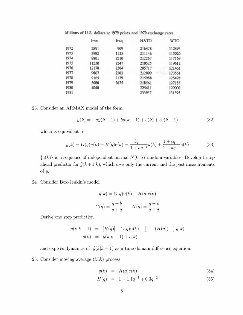
21. The English mathematician Richardson has proposed the following simple model for

the arms race between two countries

x(k + 1) = ax(k) + by(k) + f (28)

y(k + 1) = cx(k) + dy(k) + g (29)

where x(k) and y(k) are yearly expenditures on arms of the two nations and (a, b, c, d, f, g)

are model parameters. The following data has been obtained from World Armaments

and Disarmaments Year Book 1982Determine the parameters of the model by least

squares and investigate the stability of the model.

22. Consider an ARMA model of the form

y(k) = −ay(k − 1) + e(k) + ce(k − 1) (30)

which is equivalent to

y(k) = H(q)e(k) =1 + cq−1

1 + aq−1e(k) (31)

e(k) is a sequence of independent normal N(0, λ) random variables. Develop 1 step

ahead predictor for y(k+ 1|k), which uses only the current and the past measurements

of y.

7

23. Consider an ARMAX model of the form

y(k) = −ay(k − 1) + bu(k − 1) + e(k) + ce(k − 1) (32)

which is equivalent to

y(k) = G(q)u(k) +H(q)e(k) =bq−1

1 + aq−1u(k) +

1 + cq−1

1 + aq−1e(k) (33)

e(k) is a sequence of independent normal N(0, λ) random variables. Develop 1-step

ahead predictor for y(k+ 1|k), which uses only the current and the past measurements

of y.

24. Consider Box-Jenkin’s model

y(k) = G(q)u(k) +H(q)e(k)

G(q) =q + b

q + aH(q) =

q + c

q + d

Derive one step prediction

y(k|k − 1) = [H(q)]−1G(q)u(k) +[1− (H(q))−1

]y(k)

y(k) = y(k|k − 1) + e(k)

and express dynamics of y(k|k − 1) as a time domain difference equation.

25. Consider moving average (MA) process

y(k) = H(q)e(k) (34)

H(q) = 1− 1.1q−1 + 0.3q−2 (35)

8

ComputeH−1(q) as an infinite expansion by long division and develop an auto-regressive

model of the form

e(k) = H−1(q)y(k) (36)

This model facilitates estimation of noise e(k) based on current and past measurements

of y(k).

26. Given an ARMAX model of the form

y(k) =B(q)

A(q)u(k) +

C(q)

A(q)e(k) =

0.1q−1

1− 0.9q−1u(k) +

1− 0.2q−1

1− 0.9q−1e(k) (37)

Rearrange this model as

y(k) =C−1(q)B(q)

C−1(q)A(q)u(k) +

1

C−1(q)A(q)e(k) (38)

Compute C−1(q) as an infinite expansion by long division and truncate the expansion

after finite number of terms when coeffi cients become small, i.e.

C−1T (q) ≈ 1 + c1q−1 + ......+ cnq

−n (39)

Using this truncated C−1T (q), express the model in ARX form

y(k) =B(q)

A(q)u(k) +

1

A(q)e(k) (40)

A(q) = C−1T (q)A(q) ; B(q) = C−1T (q)B(q) (41)

This simple calculation will illustrate how a low order ARMAX model can be approx-

imated by a high order ARX model.

27. Consider transfer functions

G1(q) =(q − 0.5)(q + 0.5)

(q − 1)(q2 − 1.5q + 0.7)

G2(q) =(q − 0.2)(q + 0.2)

(q − 1)(q2 − 1.5q + 0.7)

H(q) =(q − 0.8)

(q2 − 1.5q + 0.7)

Derive state-space realization using observable canonical form for the following systems

(cases (a) to (d))

(a) y(k) = G1(q)u1(k) + v(k)

9

(b) y(k) = G1(q)u1(k) +G2(q)u2(k) + v(k)

(c) y(k) = G1(q)u1(k) +H(q)e(k)

(d) y(k) = G1(q)u(k) +G2(q)u(k) +H(q)e(k)

(e) Given that sequence e(k) is a zero mean white noise sequence with standarddeviation equal to 0.5, express the resulting state space models for cases (c) and

(d) in the form

x(k + 1) = Φx(k) + Γu(k) + w(k)

y(k) = Cx(k) + e(k)

and estimate covariance of white noise sequence w(k).(f) Derive state-space realization using controllable canonical form for case (a).

28. Derive a state realization for[y1(k)

y2(k)

]=

1

(q2 − 1.5q + 0.8)

[q + 0.5 q − 1.5

q − 0.5 q + 1.5

][u1(k)

u2(k)

]+

[v1(k)

v2(k)

]in controllable and observable canonical forms.

29. A system is represented by

G(s) =3

(s+ 4)(s+ 1)

(a) Derive continuous time state-space realizations

dx

dt= Ax+Bu ; y = Cx

in (a) Controllable canonical form (b) Observable canonical form

(b) Convert each of the continuous time state space models into discrete state space

form

x(k + 1) = Φx(k) +Bu(k) ; y(k) = Cx(k)

Is canonical structure in continuous time preserved after discretization? Show

that both the discrete realizations have identical transfer function G(q).

(c) If canonical structures are not preserved after discretization, derive discrete state

realizations in (a) Controllable canonical form (b) Observable canonical form

starting from G(q).

30. Derive a state realizations for[y1(t)

y2(t)

]=

1

(s2 + 3s+ 2)

[s+ 1.5 s− 2

s− 3 s+ 2

][u1(t)

u2(t)

]in controllable and observable canonical forms.

10