April 2008 To: Tom Schlafly AISC Committee on Research Subject: Progress Report No. 2 ‐ AISC Faculty Fellowship Cross‐section Stability of Structural Steel
Tom, Please find enclosed the second progress report for the AISC Faculty Fellowship. The report summarizes research efforts to study the cross‐section stability of structural steel, and to extend the Direct Strength Method to hot‐rolled steel sections. The finite strip analysis reported herein focuses on proposing simplified formulas for estimating the local buckling coefficients for all types of structural steel sections. The reported parametric studies and finite element analysis of W‐sections focus on web‐flange interaction, and comparisons of the AISC, AISI – Effective Width, and AISI – Direct Strength design methods for columns with slender cross‐sections. Sincerely,
Mina Seif ([email protected]) Graduate Research Assistant
Ben Schafer ([email protected]) Associate Professor
2
Summary of Progress
The primary goal of this AISC funded research is to study and assess the
cross‐section stability of structural steel. A timeline and brief synopsis follows.
Research begins March 2006
(Note, Mina Seif joined project in October 2006)
Progress Report #1 June 2007
Completed work:
• Performed axial and major axis bending elastic cross‐section stability analysis on the W‐ sections in the AISC (v3) shapes database using the finite strip elastic buckling analysis software CUFSM.
• Evaluated and found simple design formulas for plate buckling coefficients of W‐sections in local buckling that include web‐flange interaction.
• Reformulated the AISC, AISI, and DSM column design equations into a single notation so that the methods can be readily compared to one another, and so that the centrality of elastic buckling predictions for all the methods could be readily observed.
• Performed a finite strip elastic buckling analysis parametric study on AISC, AISI, and DSM column design equations for W‐sections to compare and contrast the design methods.
• Created educational tutorials to explore elastic cross‐section stability of structural steel with the finite strip method, tutorials include clear
3
learning objectives, step‐by‐step instructions, and complementary homework problems for students.
Papers from this research: Schafer, B.W., Seif, M.. “Cross‐section Stability of Structural Steel.” SSRC Annual Stability Conference, April 2008.
Progress Report #2 April 2008
Completed work:
• Performed axial, positive and negative major axis bending, and positive and negative minor axis bending finite strip elastic cross‐section buckling stability analysis on all the sections in the AISC (v3) shapes database using the finite strip elastic buckling analysis software CUFSM.
• Evaluated and determined simple design formulas that include web‐flange interaction for local plate buckling coefficients of all structural steel section types.
• Performed ABAQUS finite element elastic buckling analyses on W‐sections, comparing and assessing a variety of element types and mesh densities.
• Initiated an ABAQUS nonlinear finite element analysis parameter study on W‐section stub columns, and assessed and compared results to the sections strengths predicted by AISC, AISI, and DSM column design equations.

4
Table of Contents
Summary of Progress .......................................................................................................2
1 Introduction ...............................................................................................................6
2 Elastic buckling finite strip analysis of the AISC sections database and
proposed local plate buckling coefficients ....................................................................9
2.1 Objectives ...........................................................................................................9 2.2 Methodology....................................................................................................10 2.3 Results...............................................................................................................12 2.4 Development of approximate local buckling coefficients expressions ...23
3 Mesh and element sensitivity in finite element elastic buckling analysis of hot-
rolled W-section steel columns .........................................................................................40
3.1 Introduction and motivation ............................................................................40 3.2 Problem statement and modeling ................................................................41 3.3 Results and comments ......................................................................................44
3.3.1 Buckling loads ..........................................................................................44 3.3.2 Buckling modes ........................................................................................49 3.3.3 CUFSM comparison..................................................................................53
3.4 Summary and conclusions ................................................................................55 3.5 Ongoing / future work ...................................................................................55
4 FEA nonlinear collapse analysis parameter study for comparing the AISC, AISI,
and DSM design methods..............................................................................................57
4.1 Introduction and motivation .........................................................................57

5
4.2 Methodology and modeling ..........................................................................63 4.2.1 Chosen sections, dimensions, and boundary conditions ...................63 4.2.2 Parameters..................................................................................................64 4.2.3 Mesh...........................................................................................................65 4.2.4 Material modeling......................................................................................65 4.2.5 Residual stresses ........................................................................................67 4.2.6 Geometric imperfections............................................................................68
4.3 Results................................................................................................................70 4.3.1 W14 sections with variable flange thickness .............................................70 4.3.2 W14 sections with variable flange and web thicknesses at a fixed ratio ...74 4.3.3 W36 sections with variable web thickness ................................................77 4.3.4 W36 sections with variable flange and web thicknesses at a fixed ratio ...80
4.4 Ongoing / future work ...................................................................................82
5 References ................................................................................................................84

6
1 Introduction
The research work presented in this progress report represents a continuing
effort towards a fuller understanding of hot‐rolled steel cross‐sectional local
stability. Typically, locally slender cross‐sections are avoided in the design of
hot‐rolled steel structural elements, but completely avoiding local buckling
ignores the beneficial post‐buckling reserve that exists in this mode. With the
appearance of high and ultra‐high yield strength steels this practice may become
uneconomical, as the local slenderness limits for a section to remain compact are
function of the yield stress. The effect of increasing the yield strength on local
buckling is a topic that has seen some study in recent years (see e.g., Earls 1999).
Currently, the AISC employs the Q‐factor approach when slender elements exist
in the cross‐section, but analysis in Progress Report #1 indicates geometric
regions where the Q‐factor approach may be overly conservative, and other
regions where it may be moderately unconservative as well. It is postulated that
a more accurate accounting of web‐flange interaction will create a more robust
method for the design of high yield stress structural steel cross‐sections that are
locally slender.
Progress report #1 summarized how the locally slender W‐section column
design equations from the AISC Q‐factor approach, AISI Effective Width

7
Method, and AISI Direct Strength Method (DSM) can be reformulated and
arranged into a common set of notation. This common notation highlights the
central role of cross‐section stability in predicting member strength.
The first part of this document, progress report #2, provides results of finite
strip elastic cross‐section buckling analysis performed on all the sections in the
AISC (v3) shapes database (2005) under: axial, positive and negative major‐axis
bending, and positive and negative minor‐axis bending. The results are used to
evaluate the plate local buckling coefficients underlying the AISC cross‐section
compactness limits (e.g., bf/2tf and h/tw limits). In addition, the finite strip results
provide the basis for the creation of simple design formulas for local plate
buckling that include web‐flange interaction, and better represent the elastic
stability behavior of structural steel sections, for all different loading types.
The second part of this progress report provides a comparison and
assessment of the different two‐dimensional shell elements which are commonly
used in modeling structural steel. The assessment is completed through finite
element elastic buckling analysis performed on W‐sections using a variety of
element types and mesh densities in the program ABAQUS.
The final part of this report presents and discusses the initiation of a
nonlinear finite element analysis parameter study (performed in ABAQUS) on

8
W‐section stub columns. The study aims to highlight the parameters that lead to
the divergence of the section strength capacity predictions, provided by the
different design methods: AISC, AISI, and DSM column design equations.

9
2 Elastic buckling finite strip analysis of the AISC sections database and proposed local plate buckling coefficients
2.1 Objectives
Finite strip analysis was performed on all the sections of the shape database
(v3) from the AISC (2005) Manual of Steel Construction (excluding pipe sections).
The analysis was completed using CUFSM version 3.12 (Schafer and Adany
2006). Sections were simplified to their centerline geometry (the increased width
in the k‐zone was thus ignored) and analyzed under different loading conditions:
axial compression, positive and negative major‐axis bending, and positive and
negative minor‐axis bending. The analysis was used to investigate the elastic
local buckling behavior of the section (thus including web‐flange interaction) so
that the exact elastic local buckling values of the plate buckling coefficients, ck ’s,
could be compared to those underlying the AISC Specification.
Based on the exact values for elastic local buckling, approximate design
expressions that include web‐flange interaction for kc are developed for all of the
section types under compression and major‐ and minor‐axis bending.
It is noted that the finite strip method has been a reliable approach for
studying the local buckling of W‐sections, even prior to the existence of highly
10
powerful computational machines (e.g. Yoshida and Maegawa (1978) or Wang
and Rammerstorfer (1996)).
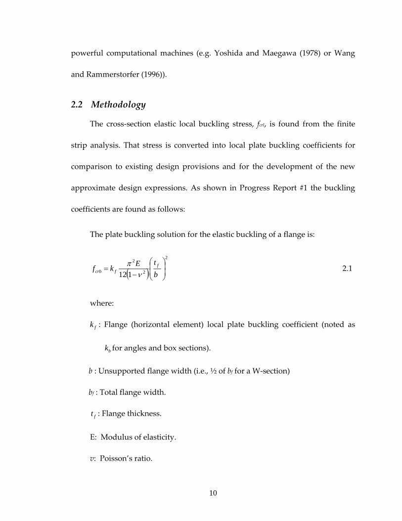
2.2 Methodology
The cross‐section elastic local buckling stress, fcrl, is found from the finite
strip analysis. That stress is converted into local plate buckling coefficients for
comparison to existing design provisions and for the development of the new
approximate design expressions. As shown in Progress Report #1 the buckling
coefficients are found as follows:
The plate buckling solution for the elastic buckling of a flange is:
( )2
2
2
112 ⎟⎟⎠
⎞⎜⎜⎝
⎛
−=
btEkf f
fcrb νπ 2.1
where:
fk : Flange (horizontal element) local plate buckling coefficient (noted as
bk for angles and box sections).
b : Unsupported flange width (i.e., ½ of bf for a W‐section)
bf : Total flange width.
ft : Flange thickness.
E: Modulus of elasticity.
v: Poisson’s ratio.

11
Setting fcrb = fcrl and solving for kf:
( ) 2
2
2112⎟⎟⎠
⎞⎜⎜⎝
⎛−=
fcrf t
bE
fkπ
νl 2.2
Similarly, the web buckling coefficient, wk , can be found, where:
( )2
2
2
112⎟⎠⎞
⎜⎝⎛
ν−π
=htEkf w
wcrh 2.3
Again, after setting fcrh = fcrl, we can solve for kw as:
( ) 2
2
2112⎟⎟⎠
⎞⎜⎜⎝
⎛π
ν−=
wcrw t
hE
fk l 2.4
where:
wk : Web (vertical element) local plate buckling coefficient (noted as dk for
angles and box sections).
h : Clear distance between flanges less the fillet (see AISC 2005).
wt : Web thickness.
Using the full cross‐section elastic local buckling stress, fcrl, the plate
buckling coefficients resulting from Equations 2.2 and 2.4 will thus include web‐
flange interaction.

12
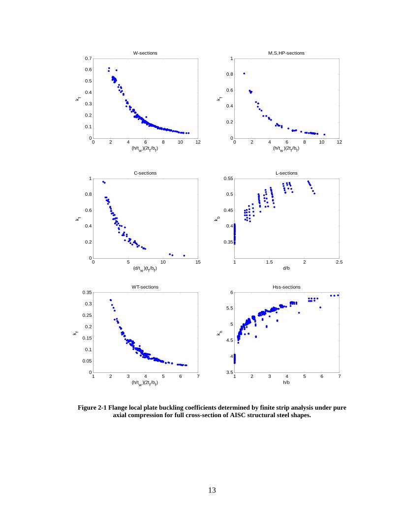
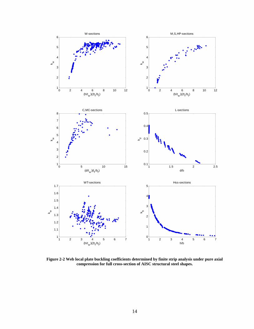
2.3 Results
Results are shown here in the form of plots of the plate buckling coefficients
versus parameters of the cross‐section geometry representing the web and flange
slenderness. The figures indicate that simple relationships exist between the
element local slenderness and the plate buckling coefficients. For example,.
Figure 2.1 shows the results for the flange (or horizontal element) buckling
coefficients, kf, for the different sections under axial compression loading. Figure
2.2 shows similar plots for the web (or vertical element) buckling coefficients.
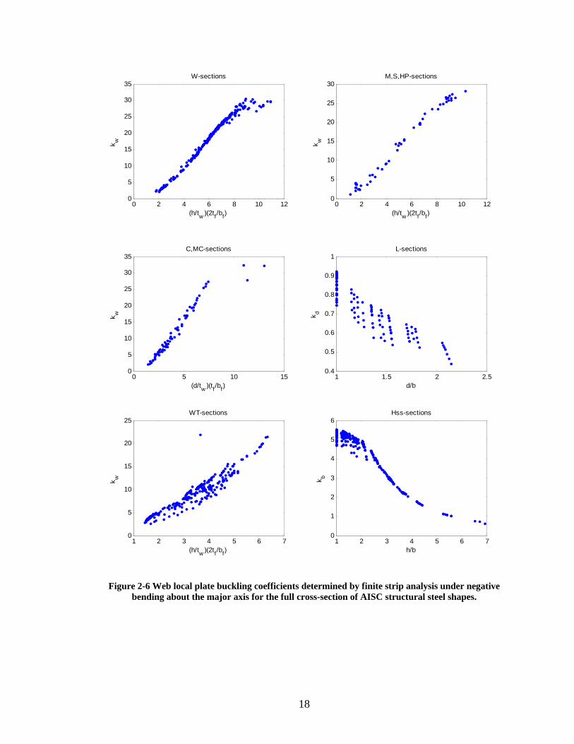
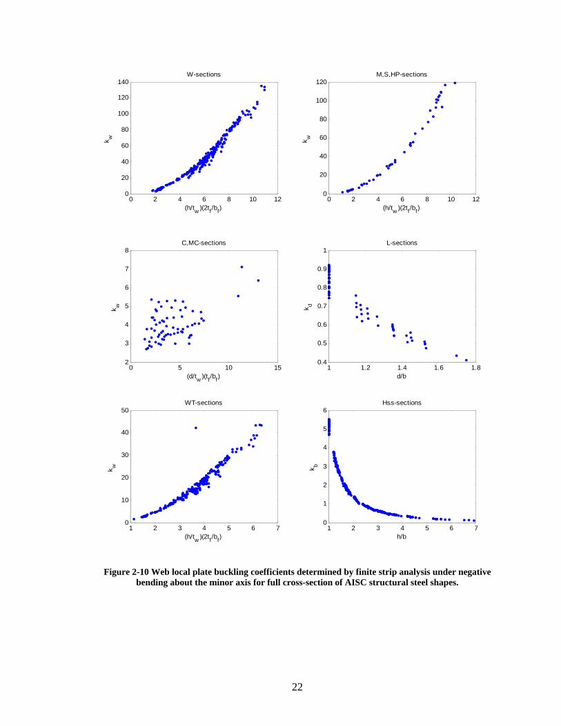
Figures 2.3 through 2.10 show the results of web and flange buckling coefficients
for the sections under various loading conditions: positive and negative major‐
axis bending, and positive and negative minor‐axis bending, respectively.
13
0 2 4 6 8 10 120
0.1
0.2
0.3
0.4
0.5
0.6
0.7W-sections
(h/tw )(2tf/bf)
k f
0 2 4 6 8 10 120
0.2
0.4
0.6
0.8
1M,S,HP-sections
(h/tw )(2tf/bf)
k f
0 5 10 150
0.2
0.4
0.6
0.8
1C-sections
(d/tw )(tf/bf)
k f
1 1.5 2 2.5
0.35
0.4
0.45
0.5
0.55L-sections
d/b
k b
1 2 3 4 5 6 70
0.05
0.1
0.15
0.2
0.25
0.3
0.35WT-sections
(h/tw )(2tf/bf)
k f
1 2 3 4 5 6 73.5
4
4.5
5
5.5
6Hss-sections
h/b
k h
Figure 2-1 Flange local plate buckling coefficients determined by finite strip analysis under pure axial compression for full cross-section of AISC structural steel shapes.
14
0 2 4 6 8 10 121
2
3
4
5
6W-sections
(h/tw )(2tf/bf)
k w
0 2 4 6 8 10 121
2
3
4
5
6M,S,HP-sections
(h/tw )(2tf/bf)
k w
0 5 10 151
2
3
4
5
6
7
8C,MC-sections
(d/tw )(tf/bf)
k w
1 1.5 2 2.50.1
0.2
0.3
0.4
0.5L-sections
d/b
k d
1 2 3 4 5 6 71
1.1
1.2
1.3
1.4
1.5
1.6
1.7WT-sections
(h/tw )(2tf/bf)
k w
1 2 3 4 5 6 70
1
2
3
4
5Hss-sections
h/b
k b
Figure 2-2 Web local plate buckling coefficients determined by finite strip analysis under pure axial compression for full cross-section of AISC structural steel shapes.

15
0 2 4 6 8 10 120.2
0.3
0.4
0.5
0.6
0.7
0.8
0.9W-sections
(h/tw )(2tf/bf)
k f
0 2 4 6 8 10 120
0.5
1
1.5
2
2.5M,S,HP-sections
(h/tw )(2tf/bf)
k f
0 5 10 150
0.2
0.4
0.6
0.8
1
1.2
1.4C,MC-sections
(d/tw )(tf/bf)
k f
1 1.1 1.2 1.3 1.41.05
1.1
1.15
1.2
1.25
1.3L-sections
d/b
k b
1 2 3 4 5 6 70
0.2
0.4
0.6
0.8
1WT-sections
(h/tw )(2tf/bf)
k f
1 2 3 4 5 6 70
5
10
15
20
25
30
35Hss-sections
h/b
k h
Figure 2-3 Flange local plate buckling coefficients determined by finite strip analysis under positive bending about the major axis for full cross-section of AISC structural steel shapes.

16
0 2 4 6 8 10 120
5
10
15
20
25
30
35W-sections
(h/tw )(2tf/bf)
k w
0 2 4 6 8 10 120
5
10
15
20
25
30
(h/tw )(2tf/bf)
k w
M,S,HP-sections
0 5 10 150
5
10
15
20
25
30
35C,MC-sections
(d/tw )(tf/bf)
k w
1 1.1 1.2 1.3 1.4
0.7
0.8
0.9
1
1.1
1.2
1.3
1.4L-sections
d/b
k d
1 2 3 4 5 6 71
1.5
2
2.5
3WT-sections
(h/tw )(2tf/bf)
k w
1 2 3 4 5 6 70
1
2
3
4
5
6Hss-sections
h/b
k b
Figure 2-4 Web local plate buckling coefficients determined by finite strip analysis under positive bending about the major axis for the full cross-section of AISC structural steel shapes.

17
0 2 4 6 8 10 120.2
0.3
0.4
0.5
0.6
0.7
0.8
0.9W-sections
(h/tw )(2tf/bf)
k f
0 2 4 6 8 10 120
0.5
1
1.5
2M,S,HP-sections
(h/tw )(2tf/bf)
k f
0 5 10 150
0.2
0.4
0.6
0.8
1
1.2
1.4C,MC-sections
(d/tw )(tf/bf)
k f
1 1.5 2 2.50.5
1
1.5
2
2.5L-sections
d/b
k b
1 2 3 4 5 6 70.4
0.6
0.8
1
1.2
1.4
1.6
1.8WT-sections
(h/tw )(2tf/bf)
k f
1 2 3 4 5 6 70
5
10
15
20
25
30
35Hss-sections
h/b
k h
Figure 2-5 Flange local plate buckling coefficients determined by finite strip analysis under negative bending about the major axis for the full cross-section of AISC structural steel shapes.
18
0 2 4 6 8 10 120
5
10
15
20
25
30
35W-sections
(h/tw )(2tf/bf)
k w
0 2 4 6 8 10 120
5
10
15
20
25
30
(h/tw )(2tf/bf)
k w
M,S,HP-sections
0 5 10 150
5
10
15
20
25
30
35C,MC-sections
(d/tw )(tf/bf)
k w
1 1.5 2 2.50.4
0.5
0.6
0.7
0.8
0.9
1L-sections
d/b
k d
1 2 3 4 5 6 70
5
10
15
20
25WT-sections
(h/tw )(2tf/bf)
k w
1 2 3 4 5 6 70
1
2
3
4
5
6Hss-sections
h/b
k b
Figure 2-6 Web local plate buckling coefficients determined by finite strip analysis under negative bending about the major axis for the full cross-section of AISC structural steel shapes.

19
0 2 4 6 8 10 120.7
0.8
0.9
1
1.1
1.2
1.3
1.4W-sections
(h/tw )(2tf/bf)
k f
0 2 4 6 8 10 121
1.1
1.2
1.3
1.4
1.5M,S,HP-sections
(h/tw )(2tf/bf)
k f
0 5 10 150.9
1
1.1
1.2
1.3
1.4
1.5
1.6C,MC-sections
(d/tw )(tf/bf)
k f
1 1.5 2 2.51
2
3
4
5L-sections
(d/b)
k b
1 2 3 4 5 6 70.9
1
1.1
1.2
1.3
1.4WT-sections
(h/tw )(2tf/bf)
k f
1 2 3 4 5 6 74.5
5
5.5
6
6.5Hss-sections
h/b
k h
Figure 2-7 Flange local plate buckling coefficients determined by finite strip analysis under positive bending about the minor axis for full cross-section of AISC structural steel shapes.

20
0 2 4 6 8 10 120
20
40
60
80
100
120
140W-sections
(h/tw )(2tf/bf)
k w
0 2 4 6 8 10 120
20
40
60
80
100
120
(h/tw )(2tf/bf)
k w
M,S,HP-sections
0 5 10 150
50
100
150
200
(d/tw )(tf/bf)
k w
C,MC-sections
1 1.5 2 2.50.9
1
1.1
1.2
1.3L-sections
d/b
k d
1 2 3 4 5 6 70
10
20
30
40
50WT-sections
(h/tw )(2tf/bf)
k w
1 2 3 4 5 6 70
1
2
3
4
5
6Hss-sections
h/b
k b
Figure 2-8 Web local plate buckling coefficients determined by finite strip analysis under positive bending about the minor axis for full cross-section of AISC structural steel shapes.

21
0 2 4 6 8 10 120.7
0.8
0.9
1
1.1
1.2
1.3
1.4W-sections
(h/tw )(2tf/bf)
k f
0 2 4 6 8 10 121
1.1
1.2
1.3
1.4
1.5M,S,HP-sections
(h/tw )(2tf/bf)
k f
0 5 10 150
0.5
1
1.5
2C,MC-sections
(d/tw )(tf/bf)
k f
1 1.2 1.4 1.6 1.80.7
0.8
0.9
1
1.1
1.2
1.3
1.4L-sections
d/b
k b
1 2 3 4 5 6 70.9
1
1.1
1.2
1.3
1.4WT-sections
(h/tw )(2tf/bf)
k f
1 2 3 4 5 6 74.5
5
5.5
6
6.5Hss-sections
h/b
k h
Figure 2-9 Flange local plate buckling coefficients determined by finite strip analysis under negative bending about the minor axis for full cross-section of AISC structural steel shapes.
22
0 2 4 6 8 10 120
20
40
60
80
100
120
140W-sections
(h/tw )(2tf/bf)
k w
0 2 4 6 8 10 120
20
40
60
80
100
120
(h/tw )(2tf/bf)
k w
M,S,HP-sections
0 5 10 152
3
4
5
6
7
8
(d/tw )(tf/bf)
k w
C,MC-sections
1 1.2 1.4 1.6 1.80.4
0.5
0.6
0.7
0.8
0.9
1L-sections
d/b
k d
1 2 3 4 5 6 70
10
20
30
40
50WT-sections
(h/tw )(2tf/bf)
k w
1 2 3 4 5 6 70
1
2
3
4
5
6Hss-sections
h/b
k b
Figure 2-10 Web local plate buckling coefficients determined by finite strip analysis under negative bending about the minor axis for full cross-section of AISC structural steel shapes.

23
2.4 Development of approximate local buckling coefficients expressions
From the results in the previous section the dependence of the local
buckling coefficients, kf and kw, on web‐flange interaction is demonstrated.
Simple functional relations exist such that the local plate buckling coefficients
can be expressed as a function of section geometry.
Note that using the same full cross‐sections elastic local buckling stress, fcrl,
instead of the individual plate buckling stresses, fcrb and fcrh, implies that
Equations 2.1 and 2.3 must be equal, thus giving a relationship between the
flange and web local buckling coefficients:
22
⎟⎟⎠
⎞⎜⎜⎝
⎛⎟⎠⎞
⎜⎝⎛=
f
wwf t
bhtkk or
22
⎟⎟⎠
⎞⎜⎜⎝
⎛⎟⎟⎠
⎞⎜⎜⎝
⎛=
w
ffw t
hbt
kk 2.5
Thus, via Equation 2.5 only one local plate buckling coefficient needs to be
determined for a cross‐section. Therefore, for each loading case, either kf or kw
was selected to develop the desired functional relation. (Furthermore, the values
of the y‐axis (k’s) were inverted for some of the cases in order to use the same
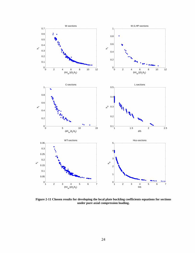
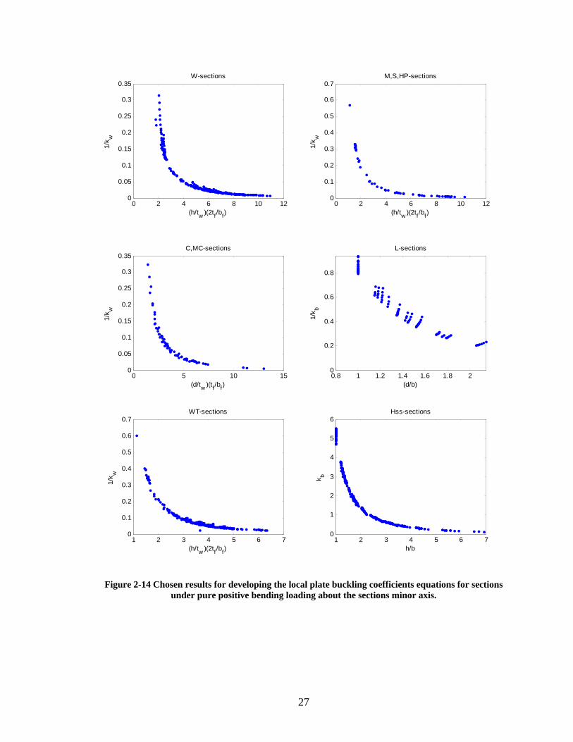
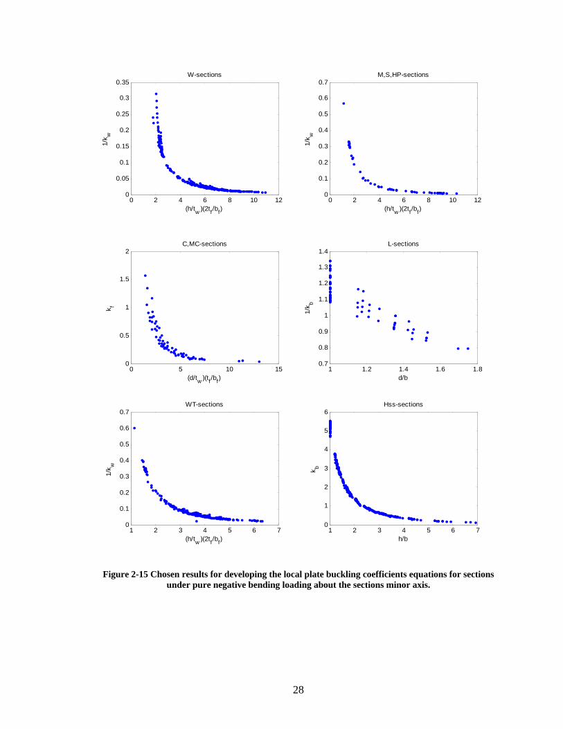
functional form for the prediction equations). Figures 2.11 through 2.15 provide
the finite strip analysis data employed for development of the empirical
prediction equations of the local plate buckling coefficients.
24
0 2 4 6 8 10 120
0.1
0.2
0.3
0.4
0.5
0.6
0.7W-sections
(h/tw )(2tf/bf)
k f
0 2 4 6 8 10 120
0.2
0.4
0.6
0.8
1M,S,HP-sections
(h/tw )(2tf/bf)
k f
0 5 10 150
0.2
0.4
0.6
0.8
1C-sections
(d/tw )(tf/bf)
k f
1 1.5 2 2.50.1
0.2
0.3
0.4
0.5L-sections
d/b
k d
1 2 3 4 5 6 70
0.05
0.1
0.15
0.2
0.25
0.3
0.35WT-sections
(h/tw )(2tf/bf)
k f
1 2 3 4 5 6 70
1
2
3
4
5Hss-sections
h/b
k b
Figure 2-11 Chosen results for developing the local plate buckling coefficients equations for sections under pure axial compression loading.

25
0 2 4 6 8 10 120
0.1
0.2
0.3
0.4
0.5W-sections
(h/tw )(2tf/bf)
1/k w
0 2 4 6 8 10 120
0.2
0.4
0.6
0.8
1
(h/tw )(2tf/bf)
1/k w
M,S,HP-sections
0 5 10 150
0.1
0.2
0.3
0.4
0.5C,MC-sections
(d/tw )(tf/bf)
1/k w
1 1.1 1.2 1.3 1.4
0.7
0.8
0.9
1
1.1
1.2
1.3
1.4L-sections
d/b
k d
1 2 3 4 5 6 70
0.2
0.4
0.6
0.8
1WT-sections
(h/tw )(2tf/bf)
k f
1 2 3 4 5 6 70
0.05
0.1
0.15
0.2
0.25Hss-sections
h/b
1/k h
Figure 2-12 Chosen results for developing the local plate buckling coefficients equations for sections under pure positive bending loading about the sections major axis.

26
0 2 4 6 8 10 120
0.1
0.2
0.3
0.4
0.5W-sections
(h/tw )(2tf/bf)
1/k w
0 2 4 6 8 10 120
0.2
0.4
0.6
0.8
1
(h/tw )(2tf/bf)
1/k w
M,S,HP-sections
0 5 10 150
0.1
0.2
0.3
0.4
0.5C,MC-sections
(d/tw )(tf/bf)
1/k w
1 1.5 2 2.50.4
0.6
0.8
1
1.2
1.4L-sections
d/b
1/k b
1 2 3 4 5 6 70
0.1
0.2
0.3
0.4WT-sections
(h/tw )(2tf/bf)
1/k w
1 2 3 4 5 6 70
0.05
0.1
0.15
0.2
0.25Hss-sections
h/b
1/k h
Figure 2-13 Chosen results for developing the local plate buckling coefficients equations for sections under pure negative bending loading about the sections major axis.
27
0 2 4 6 8 10 120
0.05
0.1
0.15
0.2
0.25
0.3
0.35W-sections
(h/tw )(2tf/bf)
1/k w
0 2 4 6 8 10 120
0.1
0.2
0.3
0.4
0.5
0.6
0.7
(h/tw )(2tf/bf)
1/k w
M,S,HP-sections
0 5 10 150
0.05
0.1
0.15
0.2
0.25
0.3
0.35
(d/tw )(tf/bf)
1/k w
C,MC-sections
0.8 1 1.2 1.4 1.6 1.8 20
0.2
0.4
0.6
0.8
L-sections
(d/b)
1/k b
1 2 3 4 5 6 70
0.1
0.2
0.3
0.4
0.5
0.6
0.7WT-sections
(h/tw )(2tf/bf)
1/k w
1 2 3 4 5 6 70
1
2
3
4
5
6Hss-sections
h/b
k b
Figure 2-14 Chosen results for developing the local plate buckling coefficients equations for sections under pure positive bending loading about the sections minor axis.
28
0 2 4 6 8 10 120
0.05
0.1
0.15
0.2
0.25
0.3
0.35W-sections
(h/tw )(2tf/bf)
1/k w
0 2 4 6 8 10 120
0.1
0.2
0.3
0.4
0.5
0.6
0.7
(h/tw )(2tf/bf)
1/k w
M,S,HP-sections
0 5 10 150
0.5
1
1.5
2C,MC-sections
(d/tw )(tf/bf)
k f
1 1.2 1.4 1.6 1.80.7
0.8
0.9
1
1.1
1.2
1.3
1.4L-sections
d/b
1/k b
1 2 3 4 5 6 70
0.1
0.2
0.3
0.4
0.5
0.6
0.7WT-sections
(h/tw )(2tf/bf)
1/k w
1 2 3 4 5 6 70
1
2
3
4
5
6Hss-sections
h/b
k b
Figure 2-15 Chosen results for developing the local plate buckling coefficients equations for sections under pure negative bending loading about the sections minor axis.

29
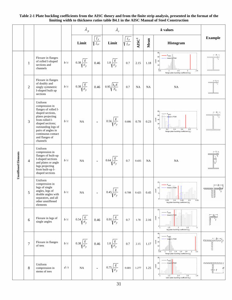
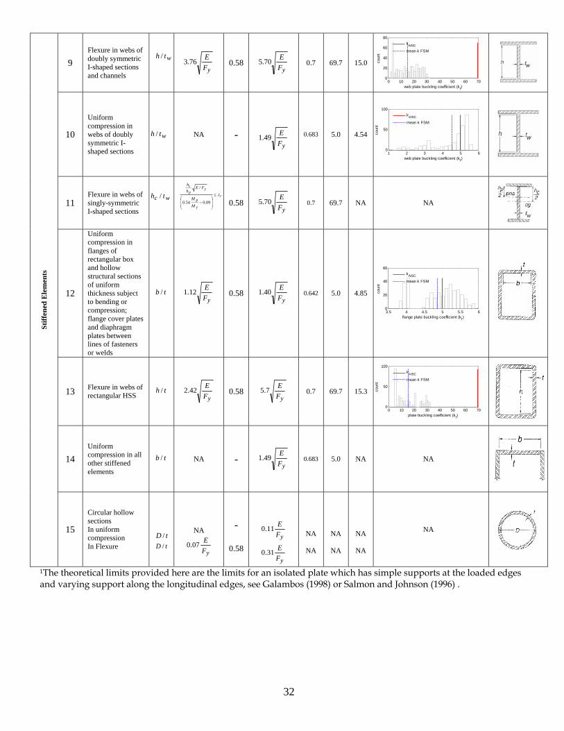
Table B4.1 in the AISC (2005) Manual of Steel Construction gives the
limiting width‐to‐thickness ratios for stiffened (e.g., webs) and unstiffened (e.g.,
flanges) compression elements in terms of pλ and rλ as functions of E and fy. A
similar table, Table 2.1, is constructed here that includes additional data:
‐ The theoretical plate buckling coefficients assumed in the AISC
Specification, as discussed, e.g., in Salmon and Johnson (1996).
‐ The theoretical cry ff / slenderness limits assumed in the AISC
Specification expressions.
‐ The average plate buckling coefficients found from the finite strip
analysis of related cross‐sections.
‐ Histograms of the related plate buckling coefficients determined
from the finite strip analysis.
Other columns in this table, including the example column, are direct
reproductions of portions of Table B4.1 of the AISC manual. From the histograms
inset in Table 2‐1 it is shown that the plate buckling coefficients fall in a wide
range, and it can be extremely approximate to represent the whole range with a
single value. The histograms also show that the AISC assumed k value is close to
the mean value from the finite strip analysis for some cases, but extremely far for
other cases.
30
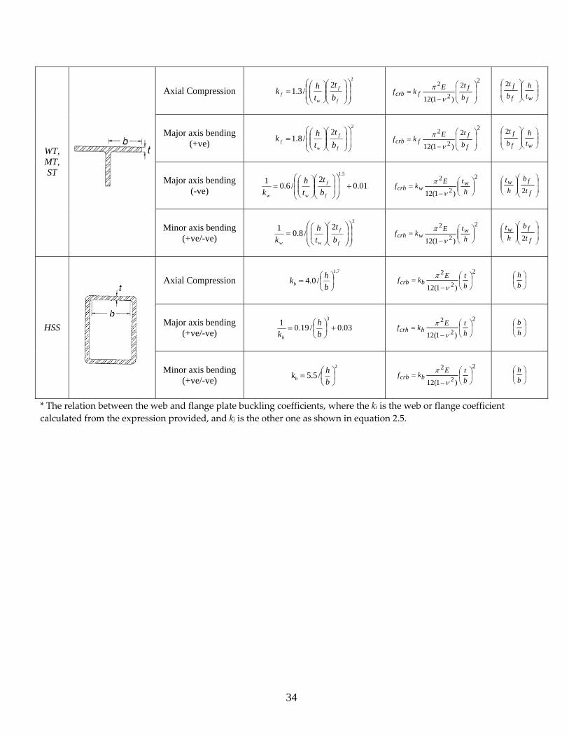
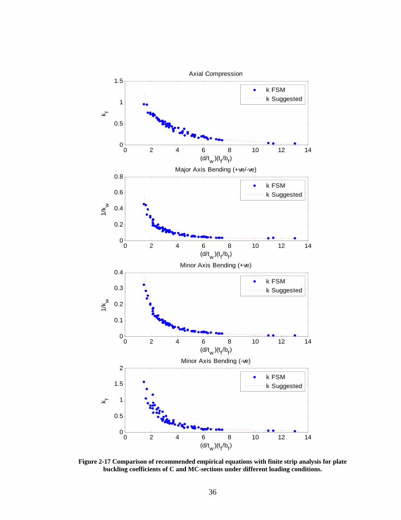
A series of simple empirical equations were developed, using the results of
Figures 2.11 through 2.15, to provide an approximate means of predicting the
local plate buckling coefficients. The equations developed were used to construct
Table 2‐2 which is essentially a proposed alternative to Table B4.1 in the AISC
manual for analyzing local stability. Table 2‐2 provides the suggested plate
buckling coefficients expressions for different section types under the different
loading cases. Finally, the expressions developed and shown in Table 2‐2 are
plotted along with the buckling coefficient values found from the finite strip
analysis in Figures 2.16 through 2.21.
31
Table 2-1 Plate buckling coefficients from the AISC theory and from the finite strip analysis, presented in the format of the limiting width to thickness ratios table B4.1 in the AISC Manual of Steel Construction
pλ rλ k values
Limit cr
yf
f
Limit cr
yf
f
AIS
C1
Mea
n
Histogram Example
1 Flexure in flanges of rolled I-shaped sections and channels
tb /
yF
E38.0 0.46 yF
E0.1 0.7 2.15 1.18
0.5 1 1.5 2 2.50
20
40
60
80
flange plate buckling coefficient (kf)
coun
t
kAISC
mean k FSM
2
Flexure in flanges of doubly and singly symmetric I-shaped built up sections
tb /
yF
E38.0 0.46L
cF
Ek95.0 0.7 NA NA NA
3
Uniform compression in flanges of rolled I-shaped sections, plates projecting from rolled I-shaped sections; outstanding legs of pairs of angles in continuous contact and flanges of channels
tb /
NA -
yFE56.0 0.686 0.70 0.23
0 0.2 0.4 0.6 0.8 10
20
40
60
80
flange plate buckling coefficient (kf)
coun
t
kAISC
mean k FSM
4
Uniform compression in flanges of built-up I-shaped sections and plates or angle legs projecting from built-up I-shaped sections
tb /
NA -
yFE64.0 0.7 0.435 NA NA
5
Uniform compression in legs of single angles, legs of double angles with separators, and all other unstiffened elements
tb /
NA -
yFE45.0 0.708 0.425 0.45
0.35 0.4 0.45 0.5 0.550
5
10
15
leg plate buckling coefficient (kf)
coun
t
kAISC
mean k FSM
6 Flexure in legs of single angles
tb /
yF
E54.0 0.46yF
E91.0 0.7 1.78 2.16
1 1.5 2 2.5 30
5
10
leg plate buckling coefficient (kf)
coun
t
kAISC
mean k FSM
7 Flexure in flanges of tees
tb /
yF
E38.0 0.46yF
E0.1 0.7 2.15 1.17
0.8 1 1.2 1.4 1.6 1.8 2 2.20
10
20
30
40
flange plate buckling coefficient (kf)
coun
t
kAISC
mean k FSM
Uns
tiffe
ned
Ele
men
ts
8 Uniform compression in stems of tees
td /
NA -
yFE75.0 0.681 1.277 1.25
1 1.2 1.4 1.6 1.80
10
20
30
stem plate buckling coefficient (kf)
coun
t
kAISC
mean k FSM
32
9 Flexure in webs of doubly symmetric I-shaped sections and channels
wth /
yFE76.3 0.58
yFE70.5 0.7 69.7 15.0
0 10 20 30 40 50 60 700
20
40
60
80
web plate buckling coefficient (kf)
coun
t
kAISC
mean k FSM
10
Uniform compression in webs of doubly symmetric I-shaped sections
wth / NA -
yFE49.1 0.683 5.0 4.54
1 2 3 4 5 60
50
100
web plate buckling coefficient (kf)
coun
t
kAISC
mean k FSM
11 Flexure in webs of singly-symmetric I-shaped sections
wc th /
r
y
p
yp
c
M
M
FEhh
λ≤
⎟⎟
⎠
⎞
⎜⎜
⎝
⎛− 09.054.0
/
0.58
yFE70.5 0.7 69.7 NA NA
12
Uniform compression in flanges of rectangular box and hollow structural sections of uniform thickness subject to bending or compression; flange cover plates and diaphragm plates between lines of fasteners or welds
tb /
yF
E12.1 0.58yF
E40.1 0.642 5.0 4.85
3.5 4 4.5 5 5.5 60
20
40
60
flange plate buckling coefficient (kf)
coun
t
kAISC
mean k FSM
13 Flexure in webs of rectangular HSS
th /
yF
E42.2 0.58yF
E7.5 0.7 69.7 15.3
0 10 20 30 40 50 60 700
50
100
plate buckling coefficient (kf)
coun
t
kAISC
mean k FSM
14 Uniform compression in all other stiffened elements
tb /
NA -
yFE49.1 0.683 5.0 NA NA
Stiff
ened
Ele
men
ts
15
Circular hollow sections In uniform compression In Flexure
tD /tD /
NA
yFE07.0
-
0.58
yFE11.0
yFE31.0
NA
NA
NA
NA
NA
NA
NA
1The theoretical limits provided here are the limits for an isolated plate which has simple supports at the loaded edges and varying support along the longitudinal edges, see Galambos (1998) or Salmon and Johnson (1996) .

33
Table 2-2 Suggested plate buckling expressions for different sections under different loading conditions
Example Loading Type Suggested k expression crf ji kk / *
Axial Compression 18.02
/5.115.2
+⎟⎟⎠
⎞⎜⎜⎝
⎛⎟⎟⎠
⎞⎜⎜⎝
⎛⎟⎟⎠
⎞⎜⎜⎝
⎛=
f
f
ww bt
th
k 2
2
2
)1(12⎟⎟⎠
⎞⎜⎜⎝
⎛
−=
htEkf w
wcrhν
π ⎟⎟
⎠
⎞
⎜⎜
⎝
⎛⎟⎟⎠
⎞⎜⎜⎝
⎛
f
fwt
bh
t2
Major axis bending (+ve/-ve) 015.0
2/5.11
2
+⎟⎟
⎠
⎞
⎜⎜
⎝
⎛⎟⎟⎠
⎞⎜⎜⎝
⎛⎟⎟⎠
⎞⎜⎜⎝
⎛=
f
f
ww bt
th
k 2
2
2
)1(12⎟⎟⎠
⎞⎜⎜⎝
⎛
−=
htEkf w
wcrhν
π ⎟⎟
⎠
⎞
⎜⎜
⎝
⎛⎟⎟⎠
⎞⎜⎜⎝
⎛
f
fwt
bh
t2
W, M, S,
HP
Minor axis bending (+ve/-ve) 008.0
2/5.11
5.2
+⎟⎟⎠
⎞⎜⎜⎝
⎛⎟⎟⎠
⎞⎜⎜⎝
⎛⎟⎟⎠
⎞⎜⎜⎝
⎛=
f
f
ww bt
th
k 2
2
2
)1(12⎟⎟⎠
⎞⎜⎜⎝
⎛
−=
htEkf w
wcrhν
π ⎟⎟
⎠
⎞
⎜⎜
⎝
⎛⎟⎟⎠
⎞⎜⎜⎝
⎛
f
fwt
bh
t2
Axial Compression 05.0/0.22.1
−⎟⎟⎠
⎞⎜⎜⎝
⎛⎟⎟⎠
⎞⎜⎜⎝
⎛⎟⎟⎠
⎞⎜⎜⎝
⎛=
f
f
wf b
ttdk
2
2
2
)1(12 ⎟⎟
⎠
⎞
⎜⎜
⎝
⎛
−=
f
ffcrb b
tEkfν
π ⎟⎟⎠
⎞⎜⎜⎝
⎛⎟⎟
⎠
⎞
⎜⎜
⎝
⎛
wf
ftd
bt
Major axis bending (+ve/-ve) 02.0/1.11
2
+⎟⎟⎠
⎞⎜⎜⎝
⎛⎟⎟⎠
⎞⎜⎜⎝
⎛⎟⎟⎠
⎞⎜⎜⎝
⎛=
f
f
ww bt
td
k 2
2
2
)1(12⎟⎟⎠
⎞⎜⎜⎝
⎛
−=
dtEkf w
wcrhν
π ⎟⎟
⎠
⎞
⎜⎜
⎝
⎛⎟⎟⎠
⎞⎜⎜⎝
⎛
f
fwtb
dt
Minor axis bending (+ve)
2
/8.01⎟⎟⎠
⎞⎜⎜⎝
⎛⎟⎟⎠
⎞⎜⎜⎝
⎛⎟⎟⎠
⎞⎜⎜⎝
⎛=
f
f
ww bt
td
k 2
2
2
)1(12⎟⎟⎠
⎞⎜⎜⎝
⎛
−=
dtEkf w
wcrhν
π ⎟⎟
⎠
⎞
⎜⎜
⎝
⎛⎟⎟⎠
⎞⎜⎜⎝
⎛
f
fwtb
dt
C, MC
Minor axis bending
(-ve)
4.2
/0.6 ⎟⎟⎠
⎞⎜⎜⎝
⎛⎟⎟⎠
⎞⎜⎜⎝
⎛⎟⎟⎠
⎞⎜⎜⎝
⎛=
f
f
wf b
ttdk
2
2
2
)1(12 ⎟⎟
⎠
⎞
⎜⎜
⎝
⎛
−=
f
ffcrb b
tEkfν
π ⎟⎟⎠
⎞⎜⎜⎝
⎛⎟⎟
⎠
⎞
⎜⎜
⎝
⎛
wf
ftd
bt
Axial Compression 3.1
/38.0 ⎟⎠⎞
⎜⎝⎛=
bdkd
2
2
2
)1(12⎟⎠
⎞⎜⎝
⎛
−=
dtEkf dcrh
ν
π ⎟⎠
⎞⎜⎝
⎛db
Major axis bending (+ve)
2
/2.1 ⎟⎠⎞
⎜⎝⎛=
bdkd
2
2
2
)1(12⎟⎠
⎞⎜⎝
⎛
−=
dtEkf dcrh
ν
π ⎟⎠
⎞⎜⎝
⎛db
Major axis bending (-ve)
3.1
/2.11⎟⎠⎞
⎜⎝⎛=
bd
kb
2
2
2
)1(12⎟⎠
⎞⎜⎝
⎛
−=
btEkf bcrb
ν
π ⎟⎠
⎞⎜⎝
⎛bd
Minor axis bending (+ve)
2
/9.01⎟⎠⎞
⎜⎝⎛=
bd
kb
2
2
2
)1(12⎟⎠
⎞⎜⎝
⎛
−=
btEkf bcrb
ν
π ⎟⎠
⎞⎜⎝
⎛bd
L
Minor axis bending (-ve)
8.0
/2.11⎟⎠⎞
⎜⎝⎛=
bd
kb
2
2
2
)1(12⎟⎠
⎞⎜⎝
⎛
−=
btEkf bcrb
ν
π ⎟⎠
⎞⎜⎝
⎛bd
34
Axial Compression 2
2/3.1 ⎟
⎟⎠
⎞⎜⎜⎝
⎛⎟⎟⎠
⎞⎜⎜⎝
⎛⎟⎟⎠
⎞⎜⎜⎝
⎛=
f
f
wf b
tthk
2
2
2 2
)1(12 ⎟⎟
⎠
⎞
⎜⎜
⎝
⎛
−=
f
ffcrb b
tEkfν
π ⎟⎟⎠
⎞⎜⎜⎝
⎛⎟⎟
⎠
⎞
⎜⎜
⎝
⎛
wf
fth
bt2
Major axis bending (+ve)
22
/8.1 ⎟⎟⎠
⎞⎜⎜⎝
⎛⎟⎟⎠
⎞⎜⎜⎝
⎛⎟⎟⎠
⎞⎜⎜⎝
⎛=
f
f
wf b
tthk
2
2
2 2
)1(12 ⎟⎟
⎠
⎞
⎜⎜
⎝
⎛
−=
f
ffcrb b
tEkfν
π ⎟⎟⎠
⎞⎜⎜⎝
⎛⎟⎟
⎠
⎞
⎜⎜
⎝
⎛
wf
fth
bt2
Major axis bending (-ve) 01.0
2/6.01
5.1
+⎟⎟⎠
⎞⎜⎜⎝
⎛⎟⎟⎠
⎞⎜⎜⎝
⎛⎟⎟⎠
⎞⎜⎜⎝
⎛=
f
f
ww bt
th
k 2
2
2
)1(12⎟⎟⎠
⎞⎜⎜⎝
⎛
−=
htEkf w
wcrhν
π ⎟⎟
⎠
⎞
⎜⎜
⎝
⎛⎟⎟⎠
⎞⎜⎜⎝
⎛
f
fwt
bh
t2
WT, MT, ST
Minor axis bending (+ve/-ve)
22
/8.01⎟⎟⎠
⎞⎜⎜⎝
⎛⎟⎟⎠
⎞⎜⎜⎝
⎛⎟⎟⎠
⎞⎜⎜⎝
⎛=
f
f
ww bt
th
k 2
2
2
)1(12⎟⎟⎠
⎞⎜⎜⎝
⎛
−=
htEkf w
wcrhν
π ⎟⎟
⎠
⎞
⎜⎜
⎝
⎛⎟⎟⎠
⎞⎜⎜⎝
⎛
f
fwt
bh
t2
Axial Compression 7.1
/0.4 ⎟⎠⎞
⎜⎝⎛=
bhkb
2
2
2
)1(12⎟⎠
⎞⎜⎝
⎛
−=
btEkf bcrb
ν
π ⎟⎠
⎞⎜⎝
⎛bh
Major axis bending (+ve/-ve) 03.0/19.01 3
+⎟⎠⎞
⎜⎝⎛=
bh
kh
2
2
2
)1(12⎟⎠
⎞⎜⎝
⎛
−=
htEkf hcrh
ν
π ⎟⎠
⎞⎜⎝
⎛hb HSS
Minor axis bending (+ve/-ve)
2
/5.5 ⎟⎠⎞
⎜⎝⎛=
bhkb
2
2
2
)1(12⎟⎠
⎞⎜⎝
⎛
−=
btEkf bcrb
ν
π ⎟⎠
⎞⎜⎝
⎛bh
* The relation between the web and flange plate buckling coefficients, where the ki is the web or flange coefficient calculated from the expression provided, and kj is the other one as shown in equation 2.5.

35
0 2 4 6 8 10 120
0.2
0.4
0.6
0.8
(h/tw )(2tf/bf)
1/k w
Axial Compression
k FSMk Suggested
0 2 4 6 8 10 120
0.2
0.4
0.6
0.8
(h/tw )(2tf/bf)
1/k w
Major Axis Bending (+ve/-ve)
k FSMk Suggested
0 2 4 6 8 10 120
0.1
0.2
0.3
0.4
(h/tw )(2tf/bf)
1/k w
Minor Axis Bending (+ve/-ve)
k FSMk Suggested
Figure 2-16 Comparison of recommended empirical equations with finite strip analysis for plate buckling coefficients of W, M, S, and HP-sections under different loading conditions.
36
0 2 4 6 8 10 12 140
0.5
1
1.5
(d/tw )(tf/bf)
k f
Axial Compression
k FSMk Suggested
0 2 4 6 8 10 12 140
0.2
0.4
0.6
0.8
(d/tw )(tf/bf)
1/k w
Major Axis Bending (+ve/-ve)
k FSMk Suggested
0 2 4 6 8 10 12 140
0.1
0.2
0.3
0.4
(d/tw )(tf/bf)
1/k w
Minor Axis Bending (+ve)
k FSMk Suggested
0 2 4 6 8 10 12 140
0.5
1
1.5
2
(d/tw )(tf/bf)
k f
Minor Axis Bending (-ve)
k FSMk Suggested
Figure 2-17 Comparison of recommended empirical equations with finite strip analysis for plate
buckling coefficients of C and MC-sections under different loading conditions.
37
1 1.2 1.4 1.6 1.8 2 2.2 2.40
0.5
1
d/b
k d
Axial Compression
k FSMk Suggested
1 1.05 1.1 1.15 1.2 1.25 1.3 1.35 1.40.5
1
1.5
d/b
k d
Major Axis Bending (+ve)
k FSMk Suggested
1 1.2 1.4 1.6 1.8 2 2.2 2.40
0.5
1
1.5
d/b
1/k b
Major Axis Bending (-ve)
k FSMk Suggested
1 1.2 1.4 1.6 1.8 2 2.2 2.40
0.5
1
1.5
(d/b)
1/k b
Minor Axis Bending (+ve)
k FSMk Suggested
1 1.1 1.2 1.3 1.4 1.5 1.6 1.7 1.80.5
1
1.5
d/b
1/k b
Minor Axis Bending (-ve)
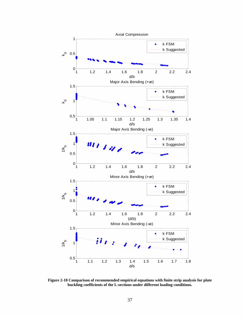
k FSMk Suggested
Figure 2-18 Comparison of recommended empirical equations with finite strip analysis for plate buckling coefficients of the L-sections under different loading conditions.
38
1 2 3 4 5 6 70
0.1
0.2
0.3
0.4
(h/tw )(2tf/bf)
k f
Axial Compression
k FSMk Suggested
1 2 3 4 5 6 70
0.5
1
(h/tw )(2tf/bf)
k f
Major Axis Bending (+ve)
k FSMk Suggested
1 2 3 4 5 6 70
0.1
0.2
0.3
0.4
(h/tw )(2tf/bf)
1/k w
Major Axis Bending (-ve)
k FSMk Suggested
1 2 3 4 5 6 70
0.2
0.4
0.6
0.8
(h/tw )(2tf/bf)
1/k w
Minor Axis Bending (+ve/-ve)
k FSMk Suggested
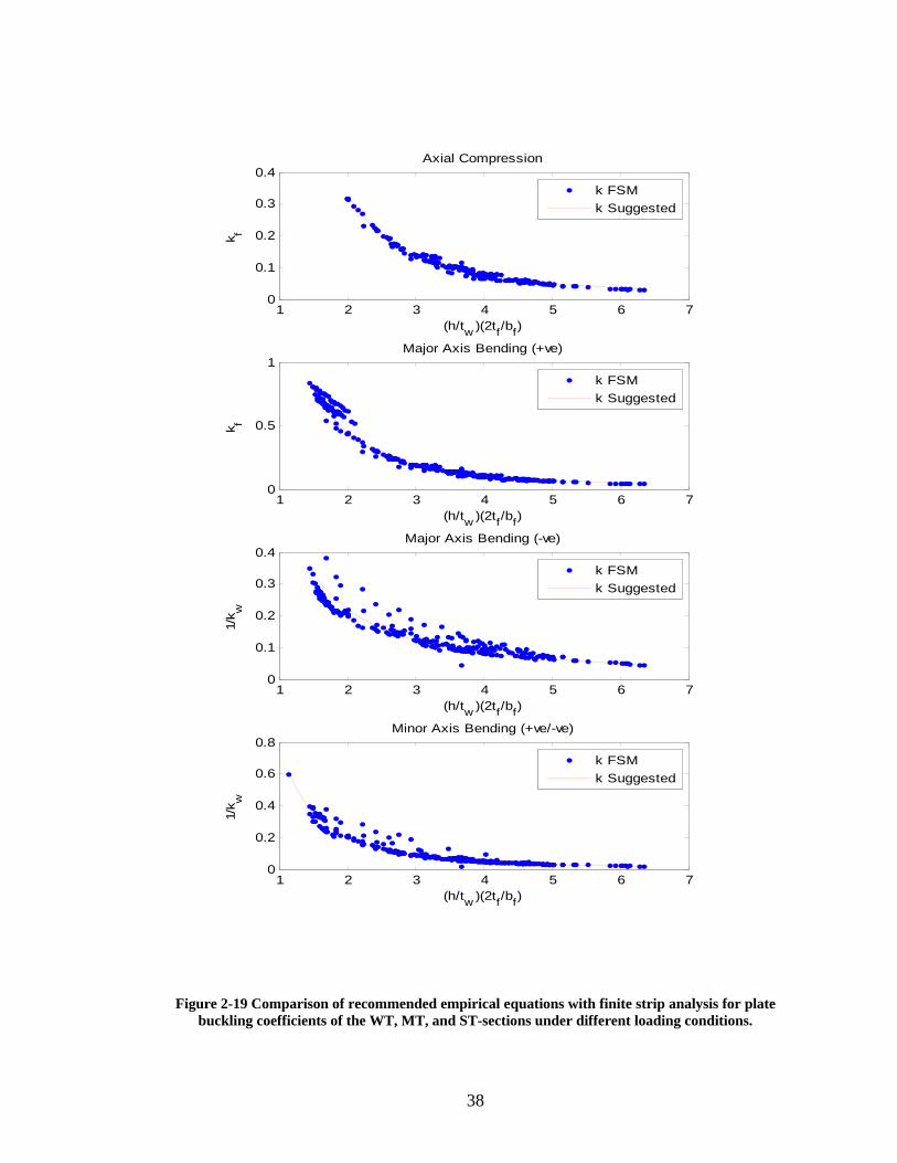
Figure 2-19 Comparison of recommended empirical equations with finite strip analysis for plate buckling coefficients of the WT, MT, and ST-sections under different loading conditions.

39
1 2 3 4 5 6 70
1
2
3
4
5
h/b
k b
Axial Compression
k FSMk Suggested
1 2 3 4 5 6 70
0.05
0.1
0.15
0.2
0.25
h/b
1/k h
Major Axis Bending (+ve/-ve)
k FSMk Suggested
1 2 3 4 5 6 70
2
4
6
h/b
k b
Minor Axis Bending (+ve/-ve)
k FSMk Suggested
Figure 2-20 Comparison of recommended empirical equations with finite strip analysis for plate buckling coefficients of the HSS-sections under different loading conditions.

40
3 Mesh and element sensitivity in finite element elastic buckling analysis of hot-rolled W-section steel columns
3.1 Introduction and motivation
The proper choice of element type and mesh refinement is a key aspect in
any finite element analysis. In structural steel analysis research, where cross-
section distortion and stability are of interest, researchers typically simplify the
cross-section as a two-dimensional model at the cross-section mid-surface and
employ shell finite elements to discretise the web and flanges. ABAQUS, which
is a widely used finite element analysis package, provides an element library that
contains a wide range of different two-dimensional shell elements. The most
commonly used shell elements are the S4, S4R, and S9R5 (as discussed below).
The S4 element has six degrees of freedom per node, adopts bilinear
interpolation for the displacement and rotation fields, incorporates finite
membrane strains, and its shear stiffness is yielded by “full” integration. The S4R
element is similar to the S4 element, except that it obtains the shear stiffness by
“reduced” integration. The S9R5 element has five degrees of freedom per node,
uses full quadratic interpolation for calculating the displacement and rotation
fields, obtains the shear stiffness by “reduced” integration, and accounts for only
“small” membrane strains. For hot-rolled structural steel sections, typically the
S4 or S4R elements are employed (with some debate between the two existing in
41
the research community) as these elements lead to slightly easier mesh
generation while adequately simulating the relevant phenomena.
It is clear from the literature that steel researchers agree that the use of S4
elements yields in stiffer members that sustain higher loads than the S4R
elements. Some, e.g. Dinis and Camotim (2006), attribute this to an “artificial”
under-estimation of the member shear stiffness in the S4R element which affects
the elements when the cross-section distorts. Others, e.g. Earls (2001), focus on
the fact that the S4 element, which is fully integrated and thus does not need
stabilization, should theoretically outperform the S4R element. However, Earls
found that within the context of the present modeling the more computationally
expensive S4 element is not required, and even yields overly stiff results,
evidenced by side-by-side comparisons between the S4 element, the S4R element,
and available experimental tests.
3.2 Problem statement and modeling
To assess and compare the different shell elements, an elastic buckling
analysis was performed on a W-section column modeled using different types
and densities of shell elements. As a reference, the section was also analyzed
using finite strip analysis, performed with CUFSM version 3.12 (Schafer and
Adany 2006).
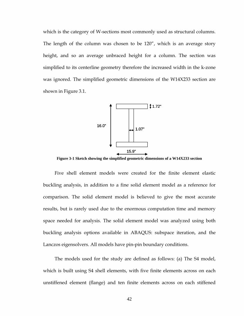
A W14X233 section was chosen for the first step of this study, as its
geometry (depth, width, and thicknesses) represents an average W14 section,
42
which is the category of W-sections most commonly used as structural columns.
The length of the column was chosen to be 120”, which is an average story
height, and so an average unbraced height for a column. The section was
simplified to its centerline geometry therefore the increased width in the k-zone
was ignored. The simplified geometric dimensions of the W14X233 section are
shown in Figure 3.1.
16.0”
1.72”
1.07”
15.9”
16.0”
1.72”
1.07”
15.9”
Figure 3-1 Sketch showing the simplified geometric dimensions of a W14X233 section
Five shell element models were created for the finite element elastic
buckling analysis, in addition to a fine solid element model as a reference for
comparison. The solid element model is believed to give the most accurate
results, but is rarely used due to the enormous computation time and memory
space needed for analysis. The solid element model was analyzed using both
buckling analysis options available in ABAQUS: subspace iteration, and the
Lanczos eigensolvers. All models have pin-pin boundary conditions.
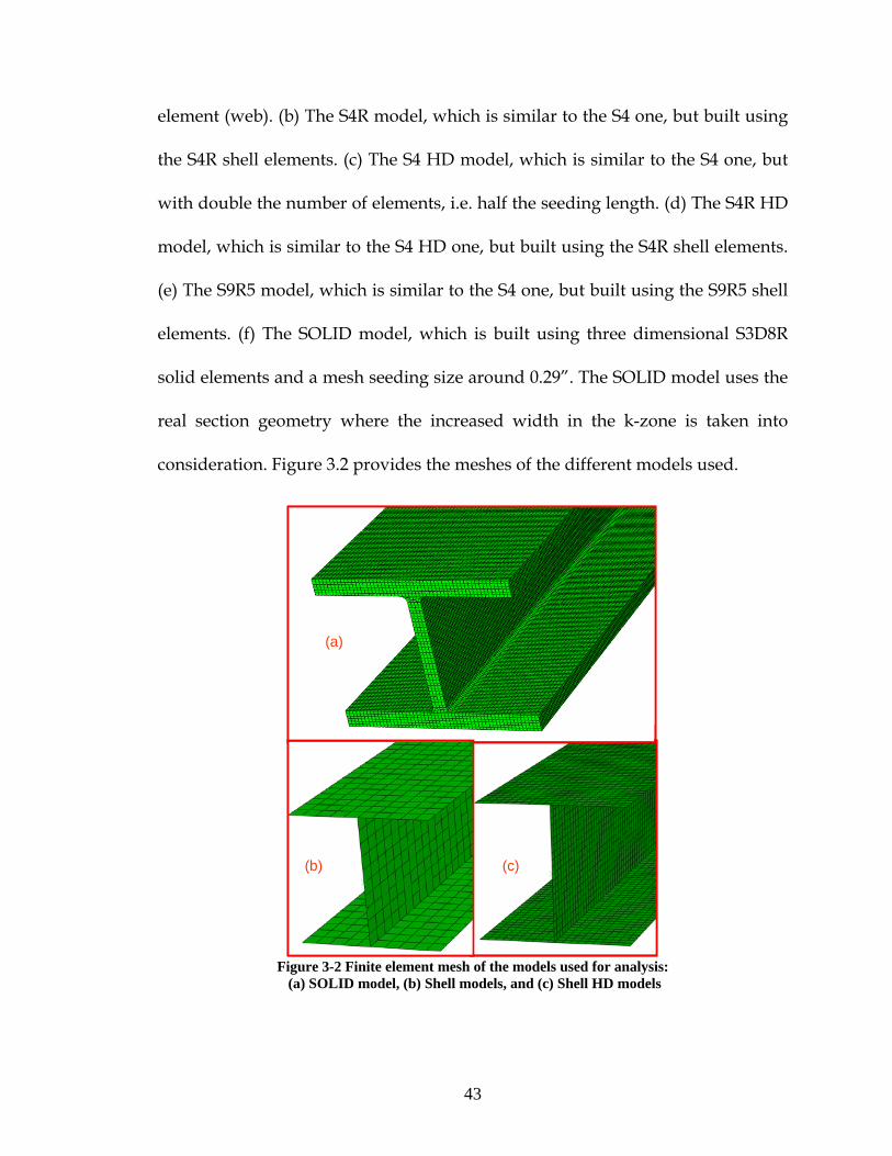
The models used for the study are defined as follows: (a) The S4 model,
which is built using S4 shell elements, with five finite elements across on each
unstiffened element (flange) and ten finite elements across on each stiffened
43
element (web). (b) The S4R model, which is similar to the S4 one, but built using
the S4R shell elements. (c) The S4 HD model, which is similar to the S4 one, but
with double the number of elements, i.e. half the seeding length. (d) The S4R HD
model, which is similar to the S4 HD one, but built using the S4R shell elements.
(e) The S9R5 model, which is similar to the S4 one, but built using the S9R5 shell
elements. (f) The SOLID model, which is built using three dimensional S3D8R
solid elements and a mesh seeding size around 0.29”. The SOLID model uses the
real section geometry where the increased width in the k-zone is taken into
consideration. Figure 3.2 provides the meshes of the different models used.
(a)
(b) (c)
(a)
(b) (c)
Figure 3-2 Finite element mesh of the models used for analysis:
(a) SOLID model, (b) Shell models, and (c) Shell HD models
44
3.3 Results and comments
3.3.1 Buckling loads
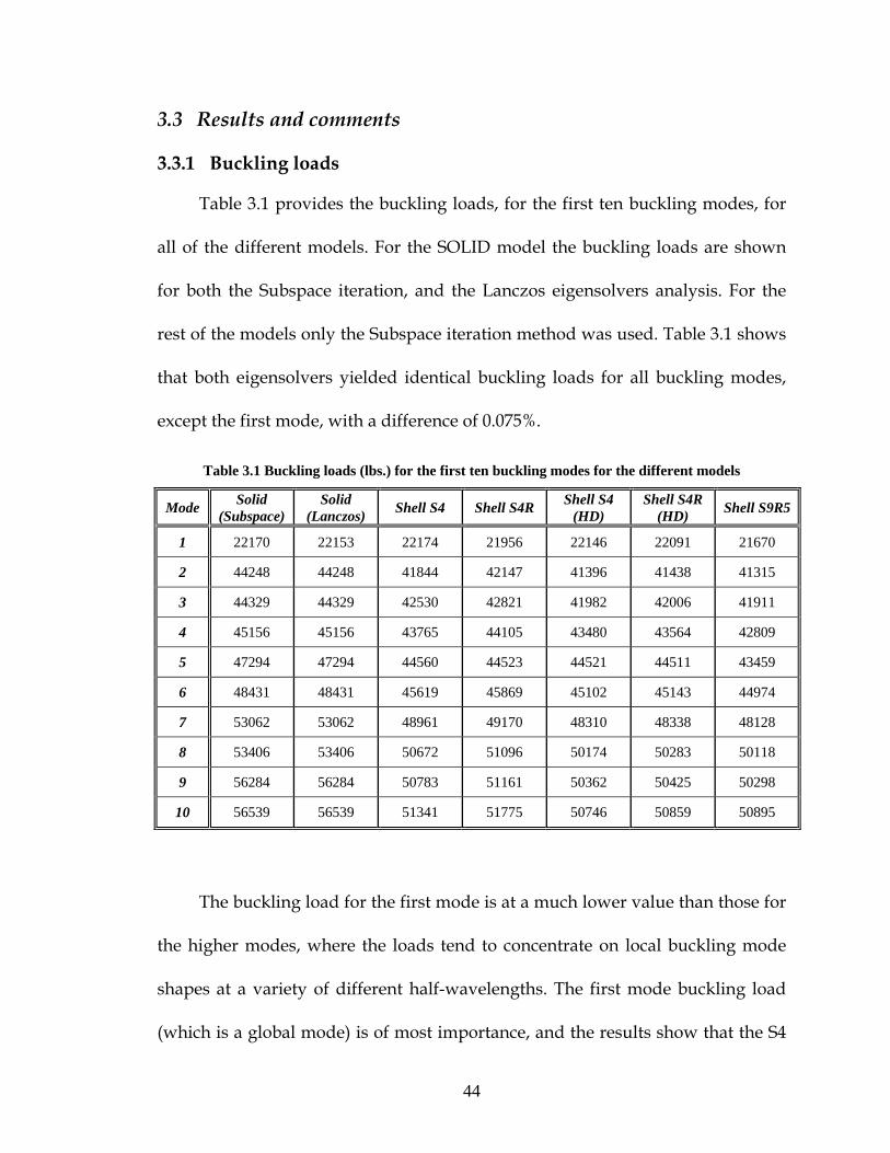
Table 3.1 provides the buckling loads, for the first ten buckling modes, for
all of the different models. For the SOLID model the buckling loads are shown
for both the Subspace iteration, and the Lanczos eigensolvers analysis. For the
rest of the models only the Subspace iteration method was used. Table 3.1 shows
that both eigensolvers yielded identical buckling loads for all buckling modes,
except the first mode, with a difference of 0.075%.
Table 3.1 Buckling loads (lbs.) for the first ten buckling modes for the different models
Mode Solid (Subspace)
Solid (Lanczos) Shell S4 Shell S4R Shell S4
(HD) Shell S4R
(HD) Shell S9R5
1 22170 22153 22174 21956 22146 22091 21670
2 44248 44248 41844 42147 41396 41438 41315
3 44329 44329 42530 42821 41982 42006 41911
4 45156 45156 43765 44105 43480 43564 42809
5 47294 47294 44560 44523 44521 44511 43459
6 48431 48431 45619 45869 45102 45143 44974
7 53062 53062 48961 49170 48310 48338 48128
8 53406 53406 50672 51096 50174 50283 50118
9 56284 56284 50783 51161 50362 50425 50298
10 56539 56539 51341 51775 50746 50859 50895
The buckling load for the first mode is at a much lower value than those for
the higher modes, where the loads tend to concentrate on local buckling mode
shapes at a variety of different half-wavelengths. The first mode buckling load
(which is a global mode) is of most importance, and the results show that the S4
45
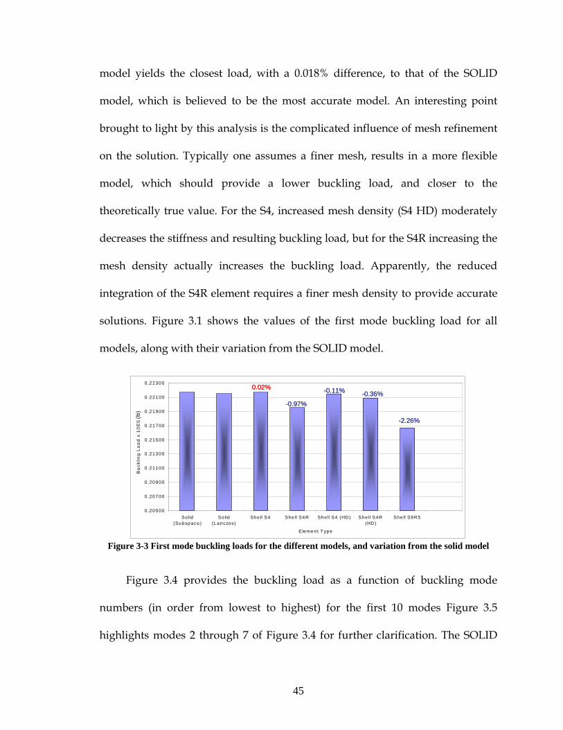
model yields the closest load, with a 0.018% difference, to that of the SOLID
model, which is believed to be the most accurate model. An interesting point
brought to light by this analysis is the complicated influence of mesh refinement
on the solution. Typically one assumes a finer mesh, results in a more flexible
model, which should provide a lower buckling load, and closer to the
theoretically true value. For the S4, increased mesh density (S4 HD) moderately
decreases the stiffness and resulting buckling load, but for the S4R increasing the
mesh density actually increases the buckling load. Apparently, the reduced
integration of the S4R element requires a finer mesh density to provide accurate
solutions. Figure 3.1 shows the values of the first mode buckling load for all
models, along with their variation from the SOLID model.
0 .20500
0 .20700
0 .20900
0 .21100
0 .21300
0 .21500
0 .21700
0 .21900
0 .22100
0 .22300
Solid(Su bsp ace)
So lid(Lanczos)
Sh e ll S4 She ll S4 R She ll S4 (HD) She ll S4R(HD)
She ll S9 R5
Eleme n t T ype
Bu
cklin
g L
oa
d x
10
E5
0.02%0.02%
-0.97%-0.97%
-0.11%-0.11% -0.36%-0.36%
-2.26%-2.26%
Figure 3-3 First mode buckling loads for the different models, and variation from the solid model
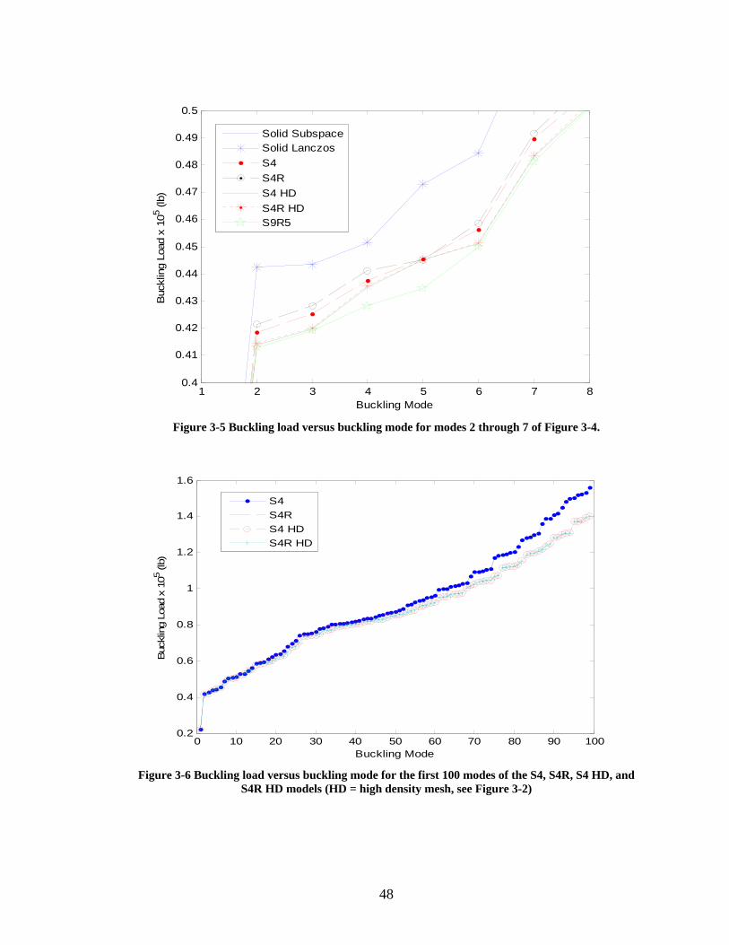
Figure 3.4 provides the buckling load as a function of buckling mode
numbers (in order from lowest to highest) for the first 10 modes Figure 3.5
highlights modes 2 through 7 of Figure 3.4 for further clarification. The SOLID
(lb)
46
model buckles at higher loads (is stiffer) than those of the other models, perhaps
due to accounting for the k-zone. (Completion of a SOLID model without the k-
zone to provide further examination of this point is planned for future research)
Interestingly, at higher buckling modes, the S4R model gives closer results to the
SOLID model than the S4, but both the S4 and S4R models yielded closer results
to the SOLID model than the S4 HD and S4R HD models - a truly counter-
intuitive result!
Figure 3.6 indicates the relation between buckling load and buckling mode
number for the first 100 buckling modes for the shell models: S4, S4R, S4 HD, and
S4R HD models. Changing the element type from S4 to S4R does not significantly
affect the results, the difference between S4 and S4R, and between S4 HD and
S4R HD is always less than 1.0%, while changing the mesh density has a much
greater effect where the differences between the S4 and S4 HD and between S4R
and S4R HD reaches the order of 15%. This is to be expected as higher modes
typically include buckling modes with short buckling wavelength and finer
meshes (the HD models) are required to accurately represent such deformations.
Dinis and Camotim (2006) indicate that for short columns where local
buckling governs, the S4 and S4R elements show practically identical results,
while for longer columns where global flexural buckling modes govern, they
give different results, with up to 20% differences. This was not observed in the

47
cases studied here, where the global flexural buckling mode governed and the
difference was less than 1.0%.
1 2 3 4 5 6 7 8 9 100.2
0.25
0.3
0.35
0.4
0.45
0.5
0.55
0.6
0.65
Buckling Mode
Buc
klin
g Lo
ad x
105 (l
b)
Solid SubspaceSolid LanczosS4S4RS4 HDS4R HDS9R5
Figure 3-4 Buckling load versus buckling mode for the first 10 modes of the different models
48
1 2 3 4 5 6 7 80.4
0.41
0.42
0.43
0.44
0.45
0.46
0.47
0.48
0.49
0.5
Buckling Mode
Buc
klin
g Lo
ad x
105 (l
b)
Solid SubspaceSolid LanczosS4S4RS4 HDS4R HDS9R5
Figure 3-5 Buckling load versus buckling mode for modes 2 through 7 of Figure 3-4.
0 10 20 30 40 50 60 70 80 90 1000.2
0.4
0.6
0.8
1
1.2
1.4
1.6
Buckling Mode
Buc
klin
g Lo
ad x
105 (l
b)
S4S4RS4 HDS4R HD
Figure 3-6 Buckling load versus buckling mode for the first 100 modes of the S4, S4R, S4 HD, and
S4R HD models (HD = high density mesh, see Figure 3-2)
49
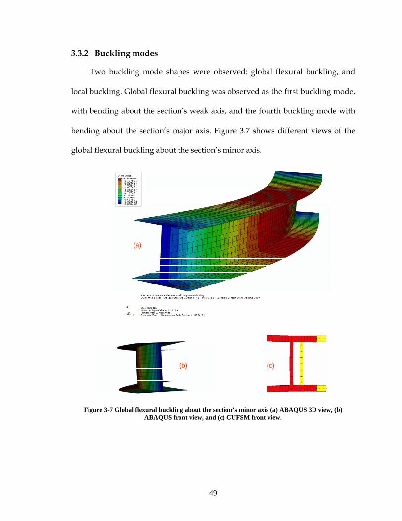
3.3.2 Buckling modes
Two buckling mode shapes were observed: global flexural buckling, and
local buckling. Global flexural buckling was observed as the first buckling mode,
with bending about the section’s weak axis, and the fourth buckling mode with
bending about the section’s major axis. Figure 3.7 shows different views of the
global flexural buckling about the section’s minor axis.
(a)
(b) (c)
(a)
(b) (c)
Figure 3-7 Global flexural buckling about the section’s minor axis (a) ABAQUS 3D view, (b)
ABAQUS front view, and (c) CUFSM front view.
50
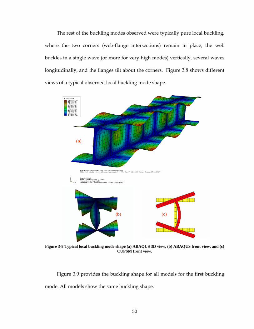
The rest of the buckling modes observed were typically pure local buckling,
where the two corners (web-flange intersections) remain in place, the web
buckles in a single wave (or more for very high modes) vertically, several waves
longitudinally, and the flanges tilt about the corners. Figure 3.8 shows different
views of a typical observed local buckling mode shape.
(a)
(b) (c)
Figure 3-8 Typical local buckling mode shape (a) ABAQUS 3D view, (b) ABAQUS front view, and (c)
CUFSM front view.
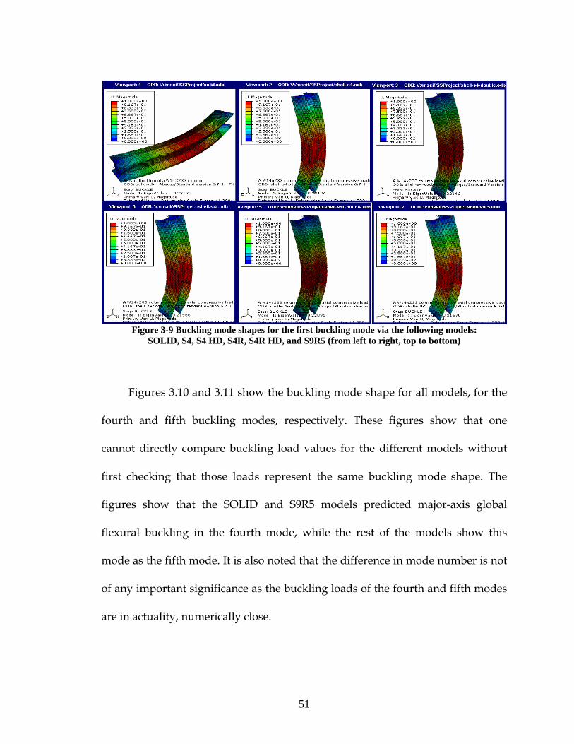
Figure 3.9 provides the buckling shape for all models for the first buckling
mode. All models show the same buckling shape.
51
Figure 3-9 Buckling mode shapes for the first buckling mode via the following models:
SOLID, S4, S4 HD, S4R, S4R HD, and S9R5 (from left to right, top to bottom)
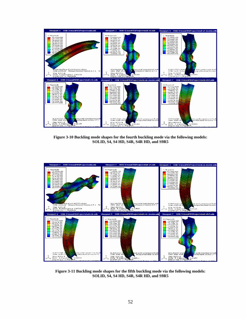
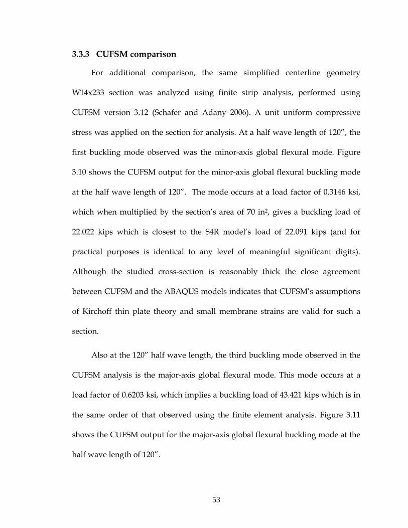
Figures 3.10 and 3.11 show the buckling mode shape for all models, for the
fourth and fifth buckling modes, respectively. These figures show that one
cannot directly compare buckling load values for the different models without
first checking that those loads represent the same buckling mode shape. The
figures show that the SOLID and S9R5 models predicted major-axis global
flexural buckling in the fourth mode, while the rest of the models show this
mode as the fifth mode. It is also noted that the difference in mode number is not
of any important significance as the buckling loads of the fourth and fifth modes
are in actuality, numerically close.
52
Figure 3-10 Buckling mode shapes for the fourth buckling mode via the following models: SOLID, S4, S4 HD, S4R, S4R HD, and S9R5
Figure 3-11 Buckling mode shapes for the fifth buckling mode via the following models: SOLID, S4, S4 HD, S4R, S4R HD, and S9R5
53
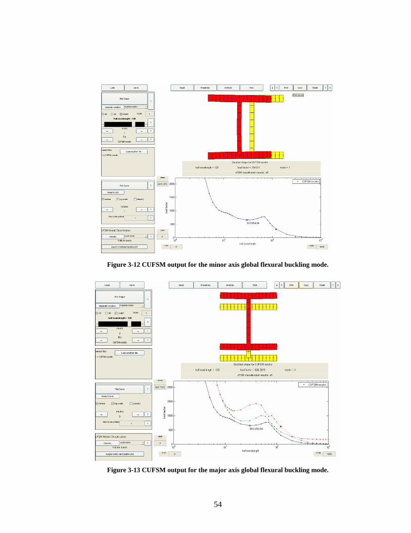
3.3.3 CUFSM comparison
For additional comparison, the same simplified centerline geometry
W14x233 section was analyzed using finite strip analysis, performed using
CUFSM version 3.12 (Schafer and Adany 2006). A unit uniform compressive
stress was applied on the section for analysis. At a half wave length of 120”, the
first buckling mode observed was the minor-axis global flexural mode. Figure
3.10 shows the CUFSM output for the minor-axis global flexural buckling mode
at the half wave length of 120”. The mode occurs at a load factor of 0.3146 ksi,
which when multiplied by the section’s area of 70 in2, gives a buckling load of
22.022 kips which is closest to the S4R model’s load of 22.091 kips (and for
practical purposes is identical to any level of meaningful significant digits).
Although the studied cross-section is reasonably thick the close agreement
between CUFSM and the ABAQUS models indicates that CUFSM’s assumptions
of Kirchoff thin plate theory and small membrane strains are valid for such a
section.
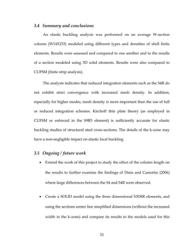
Also at the 120” half wave length, the third buckling mode observed in the
CUFSM analysis is the major-axis global flexural mode. This mode occurs at a
load factor of 0.6203 ksi, which implies a buckling load of 43.421 kips which is in
the same order of that observed using the finite element analysis. Figure 3.11
shows the CUFSM output for the major-axis global flexural buckling mode at the
half wave length of 120”.
54
Figure 3-12 CUFSM output for the minor axis global flexural buckling mode.
Figure 3-13 CUFSM output for the major axis global flexural buckling mode.
55
3.4 Summary and conclusions
An elastic buckling analysis was performed on an average W-section
column (W14X233) modeled using different types and densities of shell finite
elements. Results were assessed and compared to one another and to the results
of a section modeled using 3D solid elements. Results were also compared to
CUFSM (finite strip analysis).
The analysis indicates that reduced integration elements such as the S4R do
not exhibit strict convergence with increased mesh density. In addition,
especially for higher modes, mesh density is more important than the use of full
or reduced integration schemes. Kirchoff thin plate theory (as employed in
CUFSM or enforced in the S9R5 element) is sufficiently accurate for elastic
buckling studies of structural steel cross-sections. The details of the k-zone may
have a non-negligible impact on elastic local buckling.
3.5 Ongoing / future work
• Extend the work of this project to study the effect of the column length on
the results to further examine the findings of Dinis and Camotim (2006)
where large differences between the S4 and S4R were observed.
• Create a SOLID model using the three dimensional S3D8R elements, and
using the sections center line simplified dimensions (without the increased
width in the k‐zone) and compare its results to the models used for this

56
study to assess the effect of the k‐zone on the results and so assess the
validity of the center line geometry simplification.
• Conduct a parametric study varying the cross sections geometric
parameters, thus assessing the effect of the sections slenderness on the
results.

57
4 FEA nonlinear collapse analysis parameter study for comparing the AISC, AISI, and DSM design methods
4.1 Introduction and motivation
As discussed in Progress Report #1, a number of different methods exist for
the design of steel columns with slender cross‐sections. The three selected for
further study here are: AISC, AISI, and DSM. The AISC method, as embodied in
the 2005 AISC Specification, uses the Q‐factor approach to adjust the global
slenderness in the inelastic regime of the column curve to account for local‐global
interaction, and further uses a mixture of effective width (for stiffened elements)
and average stress (for unstiffened elements) to determine the final reduced
strength. The AISI method, from the main body of the 2007 AISI Specification for
cold‐formed steel, uses the effective width approach. In the AISI method the
global column curve is unmodified but the column area is reduced to account for
local buckling in both stiffened and unstiffened elements via the same effective
width equation. Finally, the DSM or Direct Strength Method, as given in
Appendix 1 of the 2007 AISI Specification for cold‐formed steel, uses a new
approach where the global column strength is determined and then reduced to
account for local buckling based on the local buckling cross‐section slenderness.

58
To provide more definitive comparisons between these three methods the
formulas were detailed for a centerline model of a W‐section in compression. The
formulas were presented in a common set of notation so that they may be more
directly compared. In addition, the format of presentation was modified from
that used directly in the respective Specifications so that the methods may be
most readily compared to one another and the key input parameters are brought
to light.
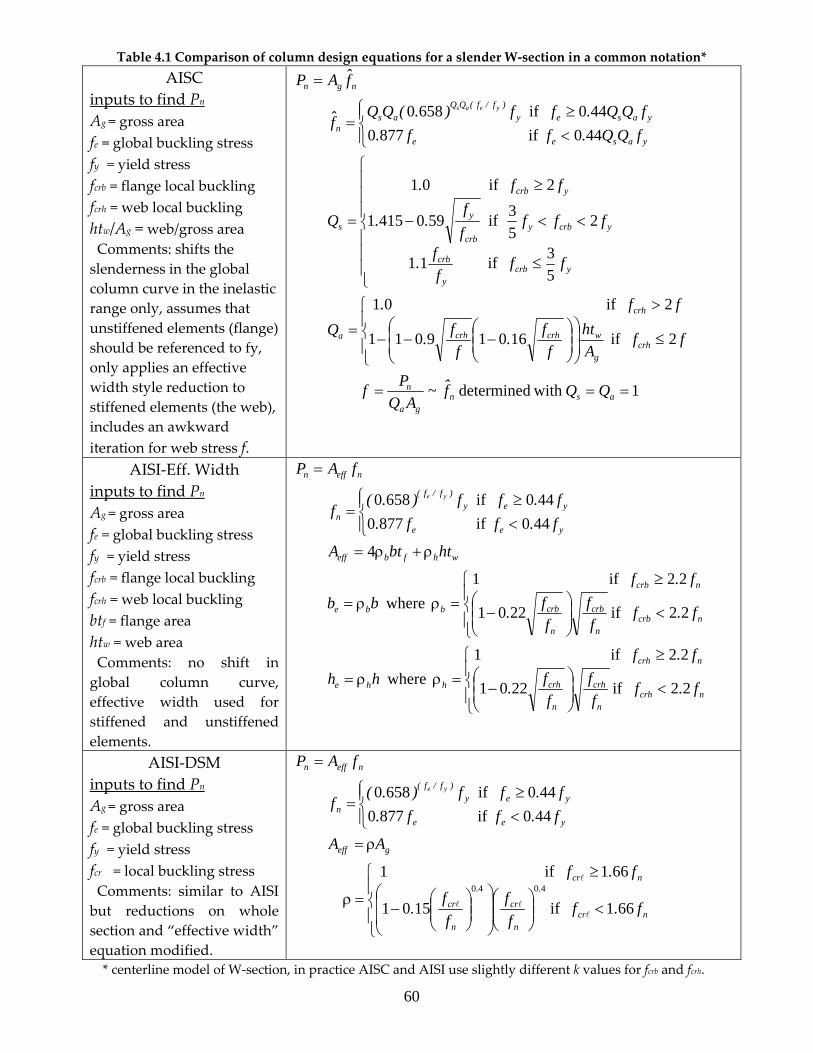
Table 4.1 shows the design equations for all three methods rearranged and
formulated into a common set of notation system as was presented in progress
report #1. Table 4.2 shows the same equations, but using the cross‐section local
buckling stress, fcrl, instead of the plate buckling stresses, fcrb and fcrh. The variables
used in the tables are defined following the tables. It is clear from the tables that
the number of free parameters in slender column design is actually significantly
less than one might typically think. Based on table 4.1, the parameters for
determining the column strength of an idealized W‐section are:
AISC: Pn/Py = f (fe/fy, fcrb/fy, fcrh/fy, htw/Ag)
AISI: Pn/Py = f (fe/fy, fcrb/fy, fcrh/fy, htw/Ag or 2bftf/Ag)
DSM: Pn/Py = f (fe/fy, fcrl/fy,)
59
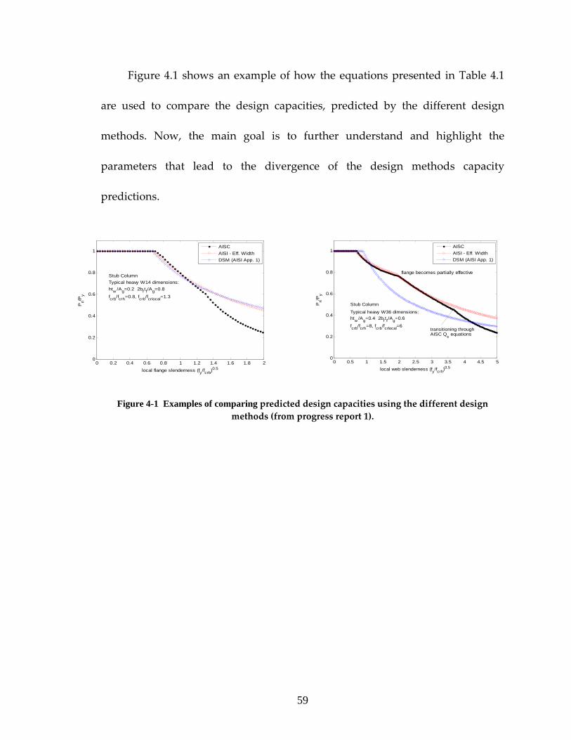
Figure 4.1 shows an example of how the equations presented in Table 4.1
are used to compare the design capacities, predicted by the different design
methods. Now, the main goal is to further understand and highlight the
parameters that lead to the divergence of the design methods capacity
predictions.
0 0.2 0.4 0.6 0.8 1 1.2 1.4 1.6 1.8 20
0.2
0.4
0.6
0.8
1
local flange slenderness (fy/fcrb)0.5
Pn/P
y
Stub ColumnTypical heavy W14 dimensions:htw /Ag=0.2 2bftf/Ag=0.8
fcrb/fcrh=0.8, fcrb/fcrlocal=1.3
AISCAISI - Eff. WidthDSM (AISI App. 1)
0 0.5 1 1.5 2 2.5 3 3.5 4 4.5 5
0
0.2
0.4
0.6
0.8
1
local web slenderness (fy/fcrh)0.5
Pn/P
y
Stub Column
Typical heavy W36 dimensions:htw /Ag=0.4 2bftf/Ag=0.6
fcrb/fcrh=8, fcrb/fcrlocal=6
flange becomes partially effective
transitioning through AISC Qs equations
AISCAISI - Eff. WidthDSM (AISI App. 1)
Figure 4-1 Examples of comparing predicted design capacities using the different design methods (from progress report 1).
60
Table 4.1 Comparison of column design equations for a slender W‐section in a common notation* AISC
inputs to find Pn Ag = gross area fe = global buckling stress fy = yield stress fcrb = flange local buckling fcrh = web local buckling htw/Ag = web/gross area Comments: shifts the slenderness in the global column curve in the inelastic range only, assumes that unstiffened elements (flange) should be referenced to fy, only applies an effective width style reduction to stiffened elements (the web), includes an awkward iteration for web stress f.
1 with determined
2 if 16019011
2 if 01
53 if 11
253 if 5904151
2 if 01
440 if 8770440 if 6580
===
⎪⎩
⎪⎨
⎧
≤⎟⎟⎠
⎞⎜⎜⎝
⎛⎟⎟⎠
⎞⎜⎜⎝
⎛−−−
>
=
⎪⎪⎪
⎩
⎪⎪⎪
⎨
⎧
≤
<<−
≥
=
⎪⎩
⎪⎨⎧
<≥
=
=
asnga
n
crhg
wcrhcrh
crh
a
ycrby
crb
ycrbycrb
y
ycrb
s
yasee
yasey)f/f(QQ
asn
ngn
QQf̂~AQ
Pf
ffAht
ff.
ff.
ff.Q
ffff.
fffff
..
ff.
Q
fQQ.ff.fQQ.ff).(QQ
f̂
f̂APyeas
AISI‐Eff. Width inputs to find Pn Ag = gross area fe = global buckling stress fy = yield stress fcrb = flange local buckling fcrh = web local buckling btf = flange area htw = web area Comments: no shift in global column curve, effective width used for stiffened and unstiffened elements.
⎪⎩
⎪⎨
⎧
<⎟⎟⎠
⎞⎜⎜⎝
⎛−
≥=ρρ=
⎪⎩
⎪⎨
⎧
<⎟⎟⎠
⎞⎜⎜⎝
⎛−
≥=ρρ=
ρ+ρ=
⎪⎩
⎪⎨⎧
<≥
=
=
ncrhn
crh
n
crh
ncrh
hhe
ncrbn
crb
n
crb
ncrb
bbe
whfbeff
yee
yey)f/f(
n
neffn
f.fff
ff.
f.fhh
f.fff
ff.
f.fbb
htbtA
f.ff.f.ff).(
f
fAPye
22 if 2201
22 if 1 where
22 if 2201
22 if 1 where
4
440 if 8770440 if 6580
AISI‐DSM inputs to find Pn Ag = gross area fe = global buckling stress fy = yield stress fcr� = local buckling stress Comments: similar to AISI but reductions on whole section and “effective width” equation modified.
661 if 1501
661 if 1
440 if 8770440 if 6580
4040
⎪⎩
⎪⎨
⎧
<⎟⎟⎠
⎞⎜⎜⎝
⎛⎟⎟
⎠
⎞
⎜⎜
⎝
⎛⎟⎟⎠
⎞⎜⎜⎝
⎛−
≥
=ρ
ρ=
⎪⎩
⎪⎨⎧
<≥
=
=
ncr
.
n
cr
.
n
cr
ncr
geff
yee
yey)f/f(
n
neffn
f.fff
ff.
f.f
AA
f.ff.f.ff).(
f
fAPye
lll
l
* centerline model of W‐section, in practice AISC and AISI use slightly different k values for fcrb and fcrh.

61
Table 4.2 Comparison of stub column design equations for a slender W‐section
when cross‐section elastic local buckling replaces isolated plate buckling solutions, i.e., fcrl = fcrb = fcrh and when global buckling is assumed to be fully braced.
AISC inputs to find Pn Ag = gross area fy = yield stress fcrl = local buckling stress htw/Ag = web/gross area Comments: adoption of fcr� for fcrb and fcrh does not simplify the AISC methodology significantly. Unstiffened and stiffened elements are treated inherently differently in the AISC methodology.
⎪⎩
⎪⎨
⎧
≤⎟⎟
⎠
⎞
⎜⎜
⎝
⎛
⎟⎟⎠
⎞⎜⎜⎝
⎛−−−
>
=
⎪⎪⎪
⎩
⎪⎪⎪
⎨
⎧
≤
<<−
≥
=
=
ycrg
w
y
cr
y
cr
ycr
a
ycry
cr
ycrycr
y
ycr
s
ygasn
ffAht
ff.
ff.
ff.
Q
ffff.
fffff
..
ff.
Q
fAQQP
2 if 16019011
2 if 01
53 if 11
253 if 5904151
2 if 01
lll
l
ll
l
l
l
AISI‐Eff. Width inputs to find Pn Ag = gross area fy = yield stress fcrl = local buckling stress Comments: when fcrl is used for fcrb and fcrh the methodology becomes the same as DSM, but with a more conservative local buckling predictor equation.
⎪⎩
⎪⎨
⎧
<⎟⎟⎠
⎞⎜⎜⎝
⎛−
≥
=ρ
ρ=
=
ycry
cr
y
cr
ycr
geff
yeffn
f.fff
ff.
f.f
AA
fAP
22 if 2201
22 if 1
lll
l
AISI‐DSM inputs to find Pn Ag = gross area fy = yield stress fcrl = local buckling stress Comments: no change from general case
661 if 1501
661 if 1
4040
⎪⎪⎩
⎪⎪⎨
⎧
<⎟⎟⎠
⎞⎜⎜⎝
⎛⎟⎟
⎠
⎞
⎜⎜
⎝
⎛
⎟⎟⎠
⎞⎜⎜⎝
⎛−
≥
=ρ
ρ=
=
ycr
.
y
cr
.
y
cr
ycr
geff
yeffn
f.fff
ff.
f.f
AA
fAP
lll
l

62
Basic definitions:
nP : Nominal section compressive strength.
gA : Gross area of the section.
b : Half of the flange width (bf = 2b).
ft : Flange thickness.
h : Height of section, between the two flange centerlines.
wt : Web thickness.
ef : Elastic global critical buckling stress, e.g., ( )2
2
rKLEπ .
L : Laterally unbraced length of the member.
r : Governing radius of gyration.
K : Effective length factor.
yf : Yield stress.
crbf : Flange elastic critical local buckling stress = ( )2
2
2
112 ⎟⎟⎠
⎞⎜⎜⎝
⎛ν−
πbtEk f
f .
crhf : Web elastic critical buckling stress = ( )2
2
2
112⎟⎠⎞
⎜⎝⎛
ν−π
htEk w
w .
fk : Flange local buckling coefficient.
wk : Web local buckling coefficient.
E : Young’s modulus of elasticity.
v : Poisson’s ratio.
lcrf : Section local buckling stress, e.g., determined by finite strip analysis.
63
aQ : Web reduction factor depends on crhf .
sQ : Flange reduction factor depends on crbf .
4.2 Methodology and modeling
A nonlinear finite element analysis parameter study is initiated for the
purpose of understanding and highlighting the parameters that lead to the
divergence between the capacity predictions of the different design methods.
4.2.1 Chosen sections, dimensions, and boundary conditions
As a first step, the analysis is conducted on stub (short) columns, avoiding
global (flexural) buckling modes, and focusing primarily on local buckling
modes. The length of the studied columns was determined according to the stub
column definitions of SSRC (i.e., Galambos 1998). For this section, W14 and W36
sections are chosen for the study, as they represent “common” sections for
columns and beams in high‐rise buildings. The W14x233 section in chosen to
represent the W14 group and the W36x330 for the W36 group, as the dimensions
of each of these sections represent approximately “average” dimensions of the
listed/available groups.
All columns are modeled with pin‐pin boundary conditions, and loaded via
applying an incremental displacement.
64
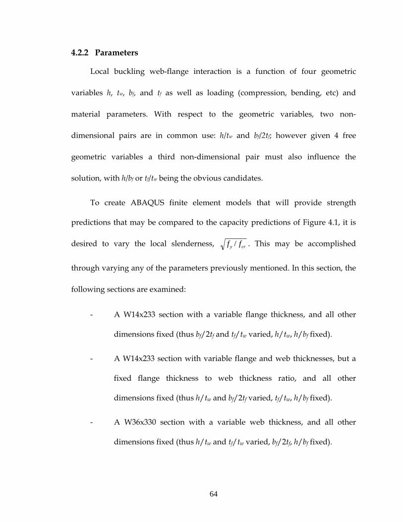
4.2.2 Parameters
Local buckling web-flange interaction is a function of four geometric
variables h, tw, bf, and tf as well as loading (compression, bending, etc) and
material parameters. With respect to the geometric variables, two non‐
dimensional pairs are in common use: h/tw and bf/2tf; however given 4 free
geometric variables a third non‐dimensional pair must also influence the
solution, with h/bf or tf/tw being the obvious candidates.
To create ABAQUS finite element models that will provide strength
predictions that may be compared to the capacity predictions of Figure 4.1, it is
desired to vary the local slenderness, cry ff / . This may be accomplished
through varying any of the parameters previously mentioned. In this section, the
following sections are examined:
‐ A W14x233 section with a variable flange thickness, and all other
dimensions fixed (thus bf/2tf and tf/tw varied, h/tw, h/bf fixed).
‐ A W14x233 section with variable flange and web thicknesses, but a
fixed flange thickness to web thickness ratio, and all other
dimensions fixed (thus h/tw and bf/2tf varied, tf/tw, h/bf fixed).
‐ A W36x330 section with a variable web thickness, and all other
dimensions fixed (thus h/tw and tf/tw varied, bf/2tf, h/bf fixed).
65
‐ A W36x330 section with variable flange and web thicknesses, but a
fixed flange thickness to web thickness ratio, and all other
dimensions fixed (thus h/tw and bf/2tf varied, tf/tw, h/bf fixed).
It is noted that decreasing an element’s thickness has an equivalent effect
on the comparison curves as increasing the material’s yield strength. For now,
thickness is used as a proxy for investigating increased element slenderness, but
future research in this area related to yield strength is required.
4.2.3 Mesh
Following the finite element analysis results presented in Section 3 of this
report, the two dimensional S4 shell element, which has six degrees of freedom
per node was chosen for the study. The S4 adopts bilinear interpolation for the
displacement and rotation fields, incorporates finite membrane strains, and shear
stiffness is yielded by “full” integration of the element. Also, informed by the
results in Section 3, the mesh density was chosen to have five S4 finite elements
across each unstiffened element (flange) and ten S4 finite elements across each
stiffened element (web). The selected mesh density is provided in Figure 4.4.
4.2.4 Material modeling
As mentioned before, increasing the material’s yield strength increases the
sections slenderness, cry ff / . For the purpose of this initial study the material
model is kept fixed at fy = 50 ksi. The material model used is similar to that of
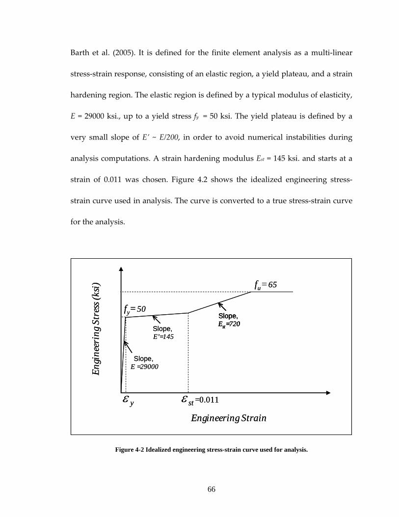
66
Barth et al. (2005). It is defined for the finite element analysis as a multi‐linear
stress‐strain response, consisting of an elastic region, a yield plateau, and a strain
hardening region. The elastic region is defined by a typical modulus of elasticity,
E = 29000 ksi., up to a yield stress fy = 50 ksi. The yield plateau is defined by a
very small slope of E’ ~ E/200, in order to avoid numerical instabilities during
analysis computations. A strain hardening modulus Est = 145 ksi. and starts at a
strain of 0.011 was chosen. Figure 4.2 shows the idealized engineering stress‐
strain curve used in analysis. The curve is converted to a true stress‐strain curve
for the analysis.
fu= 65
fy= 50
Engi
neer
ing S
tres
s (ks
i)
Engineering Strainyε stε
Slope, E =29000
Slope, Est=720Slope, Est=720
Slope, E’=145
=0.011
fu= 65
fy= 50
Engi
neer
ing S
tres
s (ks
i)
Engineering Strainyε stε
Slope, E =29000
Slope, Est=720Slope, Est=720
Slope, E’=145
=0.011
Figure 4-2 Idealized engineering stress-strain curve used for analysis.

67
4.2.5 Residual stresses
Residual stresses in hot-rolled steel are due to differential cooling (and
heating to a lesser extent) that occurs during manufacturing. These locked-in
stresses have a significant effect on the stability resistance of the column. A
variety of residual stress distributions for hot-rolled W-sections are found in
literature; Szalai and Papp (2005) studied and compared the commonly used
distributions: Young’s parabolic distribution, the ECCS linear distribution, and
Galambos and Ketter’s constant linear distribution and proposed a new
distribution. For the purposes of this work the classic and commonly used
distribution of Galambos and Ketter (1959), as shown in Figure 4.3, is employed.
The residual stresses are defined for the finite element analysis in terms of initial
stresses along longitudinal direction of the column, and given as the average
value across the element at its center, which is a common practice see, e.g., Jung
and White (2006).

68
---
--
+
yc f3.0=σ
⎟⎟⎠
⎞⎜⎜⎝
⎛
−+=
)2( fwff
ffct tdttb
tbσσ
----
---
--
+
yc f3.0=σ
⎟⎟⎠
⎞⎜⎜⎝
⎛
−+=
)2( fwff
ffct tdttb
tbσσ
----
Figure 4-3 Residual stress distribution used for analysis as given by Galambos and Ketter (1959)
4.2.6 Geometric imperfections
Nonlinearity in column response is also due to the presence of initial
geometrical imperfections, which have a significant effect on stability resistance.
The focus of this initial study is on stub columns, therefore global out-of-
plumbness and out-of-straightness imperfections are ignored and only local
imperfections are taken into consideration. Some guides, e.g. ASTM A6/A6M‐04b
(2003) show limits for manufacturing imperfections. However, it is common in
the technical literature, e.g. Kim and Lee (2002), to introduce an initial web out of
flatness of d/150 and an initial tilt in the compression flanges of bf /150. Similar
magnitudes were adopted here, though additional work in both the shape and
magnitude of imperfections is needed.

69
For the proposes of this study, the imperfections are defined for the finite
element analysis by linearly superposing a buckling eigen mode from a previous
buckling analysis. An elastic buckling analysis was performed on the W14x233
and the W36x330 stub column sections with their original dimensions. The first
buckling mode, which is a local mode, is then introduced to the model as an
initial geometric imperfection. The buckling mode introduced is scaled by a
factor that will represent the greater of: web out-of-flatness of d/150, or tilt in the
compression flange with a magnitude of bf /150. A typical local buckling mode,
and the imperfections used for the analysis are shown in Figure 4.4.

70
d
bf
bf /150
d /150
d /150
bf /150
(a)
(b)
(c)
d
bf
bf /150
d /150
d /150
bf /150
(a)
(b)
(c)
Figure 4-4 Typical local buckling mode and initial geometrical imperfections for the analysis (a) ABAQUS 3D view, (b) ABAQUS front view, and (c) CUFSM front view, with scaling factor.
4.3 Results
4.3.1 W14 sections with variable flange thickness
Models were created using the W14x233 sections dimensions, where all the
dimensions were fixed, except the flange thickness. The flange thickness was
reduced from the original thickness of 1.72” down to a thickness of 0.2”. The 0.2”
thickness is certainly not a realistic value, but is done here for the purposes of
comparing the design methods up to and through their extreme limits.
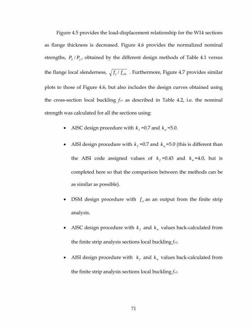
71
Figure 4.5 provides the load-displacement relationship for the W14 sections
as flange thickness is decreased. Figure 4.6 provides the normalized nominal
strengths, yn PP / , obtained by the different design methods of Table 4.1 versus
the flange local slenderness, crby ff / . Furthermore, Figure 4.7 provides similar
plots to those of Figure 4.6, but also includes the design curves obtained using
the cross-section local buckling fcrl as described in Table 4.2, i.e. the nominal
strength was calculated for all the sections using:
• AISC design procedure with fk =0.7 and wk =5.0.
• AISI design procedure with fk =0.7 and wk =5.0 (this is different than
the AISI code assigned values of fk =0.43 and wk =4.0, but is
completed here so that the comparison between the methods can be
as similar as possible).
• DSM design procedure with crf as an output from the finite strip
analysis.
• AISC design procedure with fk and wk values back-calculated from
the finite strip analysis sections local buckling fcrl.
• AISI design procedure with fk and wk values back-calculated from
the finite strip analysis sections local buckling fcrl.

72
0 0.2 0.4 0.6 0.8 1 1.2 1.4 1.6 1.8 20
500
1000
1500
2000
2500
3000
3500
4000
4500
5000
Displacement (in.)
Forc
e (k
ips)
Figure 4-5 Load-displacement relationship for the W14 sections with variable flange thickness. (Top curve represents the original W14x233 section)
0.8 1 1.2 1.4 1.6 1.8 2 2.20
0.2
0.4
0.6
0.8
1
(fy./fcrb)0.5
Pn/
Py
AISCAISIDSMABAQUS
Figure 4-6 Normalized nominal strengths obtained by the three original design methods versus the
flange local slenderness for the W14 sections with variable flange thickness.
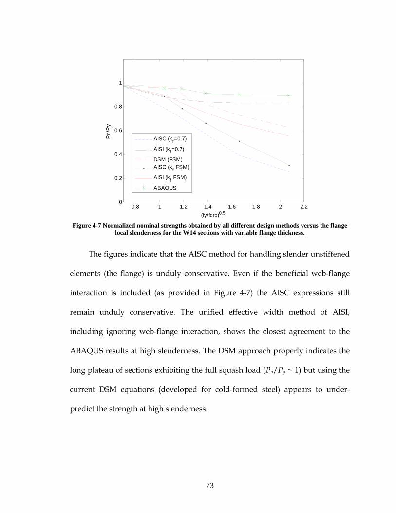
73
0.8 1 1.2 1.4 1.6 1.8 2 2.20
0.2
0.4
0.6
0.8
1
(fy/fcrb)0.5
Pn/
Py
AISC (kf=0.7)
AISI (kf=0.7)
DSM (FSM)AISC (kf FSM)
AISI (kf FSM)
ABAQUS
Figure 4-7 Normalized nominal strengths obtained by all different design methods versus the flange
local slenderness for the W14 sections with variable flange thickness.
The figures indicate that the AISC method for handling slender unstiffened
elements (the flange) is unduly conservative. Even if the beneficial web-flange
interaction is included (as provided in Figure 4-7) the AISC expressions still
remain unduly conservative. The unified effective width method of AISI,
including ignoring web-flange interaction, shows the closest agreement to the
ABAQUS results at high slenderness. The DSM approach properly indicates the
long plateau of sections exhibiting the full squash load (Pn/Py ~ 1) but using the
current DSM equations (developed for cold-formed steel) appears to under-
predict the strength at high slenderness.
74
4.3.2 W14 sections with variable flange and web thicknesses at a fixed ratio
In this small study instead of varying the flange thickness of the W14x233
both the flange and web thickness were reduced using the same fixed ratio as the
initial section. Thus h/tw and bf/2tf were increased by decreasing tf and tw, but
tf/tw held constant at a ratio of 1.607, which is the ratio for the original W14x233
dimensions.
Figure 4.8 provides the load-displacement relationship for the W14 sections
while Figures 4.9 and 4.10 provide the normalized nominal strengths, yn PP / ,
obtained by the different design methods versus the flange local slenderness,
crby ff / , for the chosen W14 sections in a similar format of that presented in
Figures 4.6 and 4.7.

75
0 0.2 0.4 0.6 0.8 1 1.2 1.4 1.6 1.8 20
500
1000
1500
2000
2500
3000
3500
4000
4500
5000
Displacement (in.)
Forc
e (k
ips)
Figure 4-8 Load-displacement relationship for the W14 sections with variable flange and web thicknesses at a fixed ratio. (Top curve represents the original W14x233 section)
0.4 0.6 0.8 1 1.2 1.4 1.6 1.8 2 2.20
0.2
0.4
0.6
0.8
1
(fy./fcrb)0.5
Pn/
Py
AISCAISIDSMABAQUS
Figure 4-9 Normalized nominal strengths obtained by the three original design methods versus the flange local slenderness for the W14 sections with variable flange and
web thicknesses at a fixed ratio.
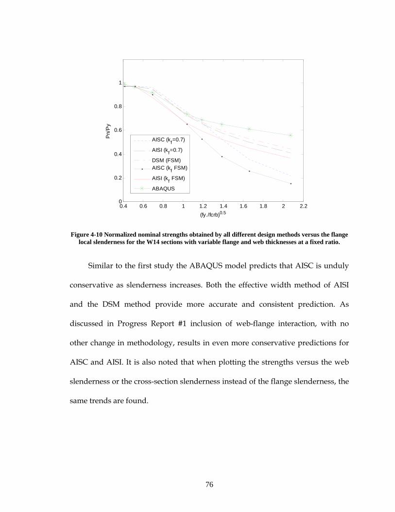
76
0.4 0.6 0.8 1 1.2 1.4 1.6 1.8 2 2.20
0.2
0.4
0.6
0.8
1
(fy./fcrb)0.5
Pn/
Py
AISC (kf=0.7)
AISI (kf=0.7)
DSM (FSM)AISC (kf FSM)
AISI (kf FSM)
ABAQUS
Figure 4-10 Normalized nominal strengths obtained by all different design methods versus the flange local slenderness for the W14 sections with variable flange and web thicknesses at a fixed ratio.
Similar to the first study the ABAQUS model predicts that AISC is unduly
conservative as slenderness increases. Both the effective width method of AISI
and the DSM method provide more accurate and consistent prediction. As
discussed in Progress Report #1 inclusion of web-flange interaction, with no
other change in methodology, results in even more conservative predictions for
AISC and AISI. It is also noted that when plotting the strengths versus the web
slenderness or the cross-section slenderness instead of the flange slenderness, the
same trends are found.
77
4.3.3 W36 sections with variable web thickness
Similar to the previous parameter studies on the W14 sections, similar
studies were completed using a W36x330 as the base section. For the first W36
study, the web slenderness was varied by fixing all of the cross-section
dimensions except the web thickness. The web thickness was reduced from the
original thickness of 1.02” down to a thickness of 0.1”. As before, the 0.1”
thickness is not intended to be a practical value, but is used here for the purposes
of exercising the design methods up to and through their limits.
Figure 4.11 provides the load-displacement relationship for the W36
sections used. Figures 4.12 shows the normalized nominal strengths, yn PP / ,
obtained by the different design methods versus the web local slenderness,
crhy ff / , for the chosen W36 sections in a similar format of that presented for
the W14 sections previously.

78
0 0.2 0.4 0.6 0.8 1 1.2 1.4 1.6 1.8 20
500
1000
1500
2000
2500
3000
3500
4000
4500
5000
Displacement (in.)
Forc
e (k
ips)
Figure 4-11 Load-displacement relationship for the W36 sections with variable web thickness. (Top curve represents the original W36x330 section)
1 2 3 4 5 6 7 80
0.2
0.4
0.6
0.8
1
(fy/fcrh)0.5
Pn/
Py
AISCAISIDSMABAQUS
Figure 4-12 Normalized nominal strengths obtained by the three original design methods versus the web local slenderness for the W36 sections with variable web thickness.
79
The ABAQUS analysis indicates that as the web thickness is decreased the
W36 section is still able to nearly reach its squash load. The AISC and AISI
methods generally agree with the predicted ABAQUS strength, while DSM does
not. In fact DSM predicts strong reductions in the cross-section strength which
are not realized. In this case, the presumption that the local buckling of the web
initiates a similar local buckling in the flange does not occur. Examination of the
local buckling mode shape shows that the local buckling is primarily one of web
local buckling with little flange deformation. DSM’s assumption, driven from
elastic stability analysis, that member local buckling and element local buckling
are one in the same does not happen in this section. The case where the web is
significantly more slender than the flange (tf/tw far from 1) requires further
investigation.
It is worth noting that this phenomenon (where DSM provides overly
conservative predictions) exists in cold-formed steel members (which are of
constant thickness) when one element is significantly wider than another. In
these cases it has been found that although DSM is conservative, such sections
also have significant serviceability problems. Such sections with highly varying
element slenderness typically benefit from the inclusion of a longitudinal
stiffener which provides a significant boost to the elastic buckling of the slender
element. Nonetheless, this phenomenon needs further study before DSM can be
fully realized in structural steel.
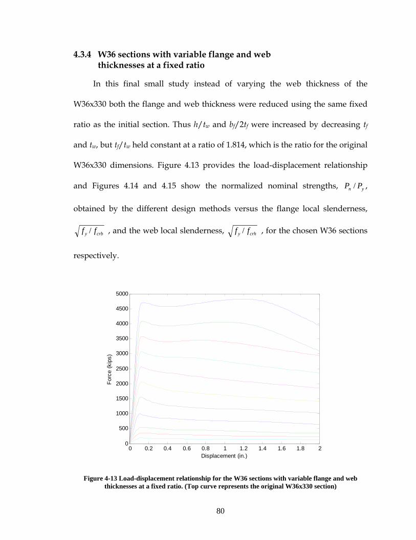
80
4.3.4 W36 sections with variable flange and web thicknesses at a fixed ratio
In this final small study instead of varying the web thickness of the
W36x330 both the flange and web thickness were reduced using the same fixed
ratio as the initial section. Thus h/tw and bf/2tf were increased by decreasing tf
and tw, but tf/tw held constant at a ratio of 1.814, which is the ratio for the original
W36x330 dimensions. Figure 4.13 provides the load-displacement relationship
and Figures 4.14 and 4.15 show the normalized nominal strengths, yn PP / ,
obtained by the different design methods versus the flange local slenderness,
crby ff / , and the web local slenderness, crhy ff / , for the chosen W36 sections
respectively.
0 0.2 0.4 0.6 0.8 1 1.2 1.4 1.6 1.8 20
500
1000
1500
2000
2500
3000
3500
4000
4500
5000
Displacement (in.)
Forc
e (k
ips)
Figure 4-13 Load-displacement relationship for the W36 sections with variable flange and web thicknesses at a fixed ratio. (Top curve represents the original W36x330 section)

81
0.5 1 1.5 2 2.50
0.2
0.4
0.6
0.8
1
(fy/fcrb)0.5
Pn/
Py
AISC (kf=0.7)
AISI (kf=0.7)
DSM (FSM)AISC (kf FSM)
AISI (kf FSM)
ABAQUS
Figure 4-14 Normalized nominal strengths obtained by all different design methods versus the flange local slenderness for the W36 sections with variable flange and web thicknesses at a fixed ratio.
1 2 3 4 5 6 7 80
0.1
0.2
0.3
0.4
0.5
0.6
0.7
0.8
0.9
1
(fy/fcrh)0.5
Pn/
Py
AISC (kw =5.0)
AISI (kw =5.0)
DSM (FSM)AISC (kw FSM)
AISI (kw FSM)
ABAQUS
Figure 4-15 Normalized nominal strengths obtained by all different design methods versus the web local slenderness for the W36 sections with variable flange and web thicknesses at a fixed ratio
82
As shown in Figure 4-14 and 4-15 AISC’s predicted stub column strength is
in poor agreement with the ABAQUS predictions. For the conventional W36x330
AISC and ABAQUS essentially predict the squash load, but as the section is
made more slender AISC first over-predicts (unconservative) and then under-
predicts the strength. AISI’s effective width methodology has good agreement
with the observed strength. DSM exhibits the same trend as observed in the
ABAQUS models, but provides an overly conservative prediction. Inclusion of
elastic web-flange interaction in either the AISC or AISI methodologies leads to
even more conservative predictions.
4.4 Ongoing / future work
The work reported in this section represents only the initiation of the
nonlinear finite element studies anticipated for this projection. Additional planne
work includes:
• Further investigate the results presented in this section and understand
their relationships and their effects on the sections buckling stability.
• Extend the work initiated herein on the W14 and W36 sections to include a
wider range of W‐sections and other section types.
• Expand the finite element parameter study initiated herein, to include
studying:
83
‐ The effect of more section geometric parameters and columns
lengths.
‐ The effect of different material models; elastic regions, strength, and
strain hardenings.
‐ The effect of different types, shapes, and scales of initial geometric
imperfections.
‐ The effect of using different residual stress distributions.
‐ Different boundary conditions and loading cases.
• Propose design improvements to the DSM design procedure for its
application to structural steel.
• Explore the possibility of modifications to a small group of standard cross
sections that will be more appropriate for higher yield stress applications,
taking advantage of the beneficial post‐buckling reserve.

84
5 References Ádány, S., Schafer, B.W. (2007). “A full modal decomposition of thin‐walled, single‐branched open cross‐section members via the constrained finite strip method.” Elsevier, Journal of Constructional Steel Research (In Press 2007). AISC (2005). “Specification for Structural Steel Buildings”, American Institute of Steel Construction, Chicago, IL. ANSI/ASIC 360‐05. AISI (2007). “North American Specification for the Design of Cold‐Formed Steel Structures”, American Iron and Steel Institute, Washington, D.C., AISI‐S100. ASTM (2003), “Standard Specification for General Requirements for Rolled Structural Steel Bars, Plates, Shapes, and Sheet Piling”, ASTM A6/A6M‐04b, American Society for Testing and Materials, West Conshohocken, PA. Axhag, F., Johansson, B. (1999). “Tension flange instability of I‐beams”, Journal of onstructional Steel Research 49 (1999) 69–81. Barth, K.E. et al (2005). “Evaluation of web compactness limits for singly and doubly symmetric steel I‐girders”, Journal of Constructional Steel Research 61 (2005) 1411–1434. Dinis, P.B., Camotim, D. (2006). “On the use of shell finite element analysis to assess the local buckling and post‐buckling behavior of cold‐formed steel thin‐walled members”, III European Conference on Computational Mechanics Solids, Structures and Coupled Problems in Engineering C.A. Mota Soares et.al. (eds.) Lisbon, Portugal, 5–8 June 2006. Earls, C.J. (1999). “On the inelastic failure of high strength steel I‐shaped beams”, Journal of Constructional Steel Research 49 (1999) 1–24. Earls, C.J. (2001). “Constant moment behavior of high‐performance steel I‐shaped beams”, Journal of Constructional Steel Research 57 (2001) 711–728. Galambos, T.V., Ketter, R.L. (1959). “Columns under combined bending and thrust”, Journal Engineering Mechanics Division, ASCE 1959; 85:1–30.

85
Galambos, T. (1998). “Guide to Stability Design Criteria for Metal Structures”. 5th ed., Wiley, New York, NY, 815‐822. Jung, S., White, D.W. (2006). “Shear strength of horizontally curved steel I‐girders—finite element analysis studies”, Journal of Constructional Steel Research 62 (2006) 329–342. Kim, S., Lee, D. (2002). “Second‐order distributed plasticity analysis of space steel frames”, Engineering Structures 24 (2002) 735–744. Salmon, C.G., Johnson, J.S. (1996). “Steel structures: design and behavior: emphasizing load and resistance factor design” HarperCollins College Publishers, New York, NY. Schafer, B.W., Ádány, S. (2005). “Understanding and classifying local, distortional and global buckling in open thin‐walled members.” Proceedings of the Structural Stability Research Council Annual Stability Conference, May, 2005. Montreal, Quebec, Canada. 27‐46. Schafer, B.W., Ádány, S. (2006). “Buckling analysis of cold‐formed steel members using CUFSM: conventional and constrained finite strip methods.” Proceedings of the Eighteenth International Specialty Conference on Cold‐Formed Steel Structures, Orlando, FL. 39‐54. Schafer, B.W., Seif, M. (2007). “Cross‐section Stability of Structural Steel.” American Institute of Steel Construction, Progress Report No. 1. AISC Faculty Fellowship, 25 June 2007. Schafer, B.W., Seif, M. (2008) “Cross‐section Stability of Structural Steel.” SSRC Annual Stability Conference, April 2008. Szalai, J., Papp, F. (2005). “A new residual stress distribution for hot‐rolled I‐shaped sections”, Journal of Constructional Steel Research 61 (2005) 845–861. Wang, X., Rammerstorfer, F.G. (1996). “Determination of Effective Breadth and Effective Width of Stiffened Plates by Finite Strip Analyses”, Thin‐Walled Structures Vol. 26, No. 4, pp. 261‐286, 1996. Yoshida, H., Maegawa, K. (1978). “Local and Member Buckling of H‐Columns”, Journal of Structural Mechanics, (1978), 6(1), 1‐27.
Recommended