Diversification and Portfolios
Economics 71a: Spring 2007
Mayo chapter 8Malkiel, Chap 9-10Lecture notes 3.2b
Goals
Portfolios and correlationsDiversifiable versus nondiversifiable riskCAPM and Beta
Capital asset pricing model Is the CAPM really useful?Asset allocation
Risk: Individual->Portfolio
Early models Risk is based on each individual stock
Modern approaches Consider how it effects “portfolio” of
holdings Markowitz Modern portfolio theory Diversification
Diversification and Portfolios
“Don’t put all your eggs in one basket”Buying a large set of securities can
reduce risk
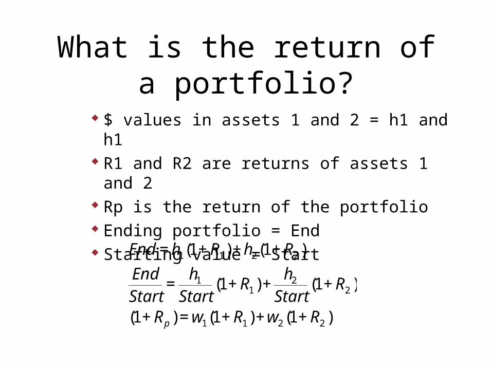
What is the return of a portfolio?
$ values in assets 1 and 2 = h1 and h1 R1 and R2 are returns of assets 1 and 2 Rp is the return of the portfolio Ending portfolio = End Starting value = Start
€
End = h1(1+ R1)+h2(1+ R2 )
EndStart
=h1
Start(1+ R1)+
h2
Start(1+ R2 )
(1+ Rp ) =w1(1+ R1)+w2(1+ R2 )
In words
The return of a portfolio is equal to a weighted average of the returns of each investment in the portfolio
The weight is equal to the fraction of wealth in each investment
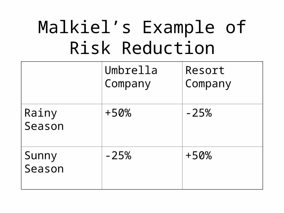
Malkiel’s Example of Risk ReductionUmbrella Company
Resort Company
Rainy Season +50% -25%
Sunny Season -25% +50%
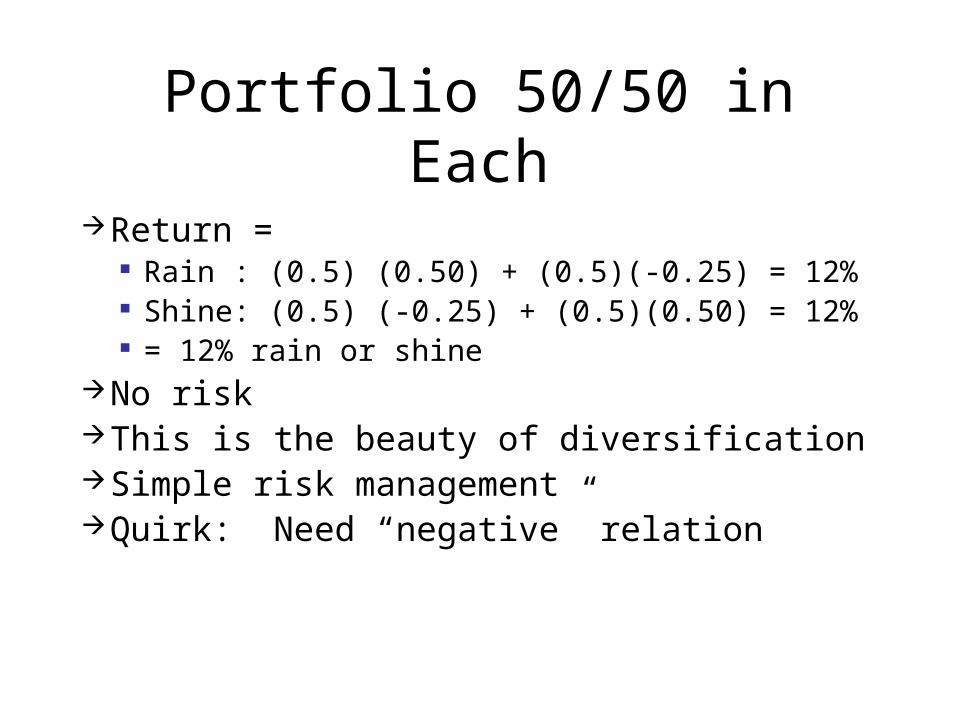
Portfolio 50/50 in Each
Return = Rain : (0.5) (0.50) + (0.5)(-0.25) = 12% Shine: (0.5) (-0.25) + (0.5)(0.50) = 12% = 12% rain or shine
No riskThis is the beauty of diversificationSimple risk managementQuirk: Need “negative” relation
What is going on?
Asset returns have perfect “negative correlation”
They move exactly opposite to each other
Is this always necessary? No
Diversification Experiment
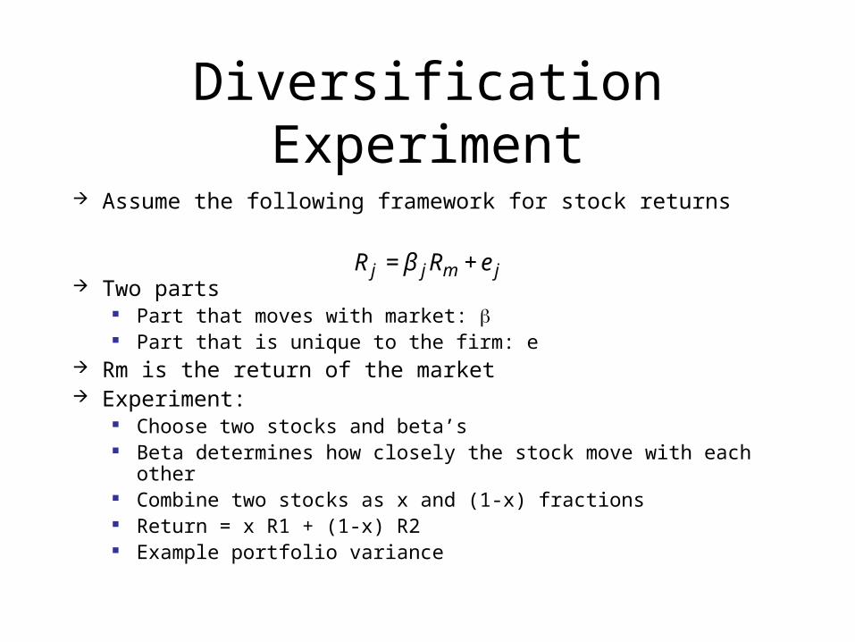
Assume the following framework for stock returns
Two parts Part that moves with market: Part that is unique to the firm: e
Rm is the return of the market Experiment:
Choose two stocks and beta’s Beta determines how closely the stock move with each other Combine two stocks as x and (1-x) fractions Return = x R1 + (1-x) R2 Example portfolio variance
€
R j = β jRm + e j
Web Examples
See multi-Beta scatter plots Portfolio 2
Quick Application: A perfect hedge
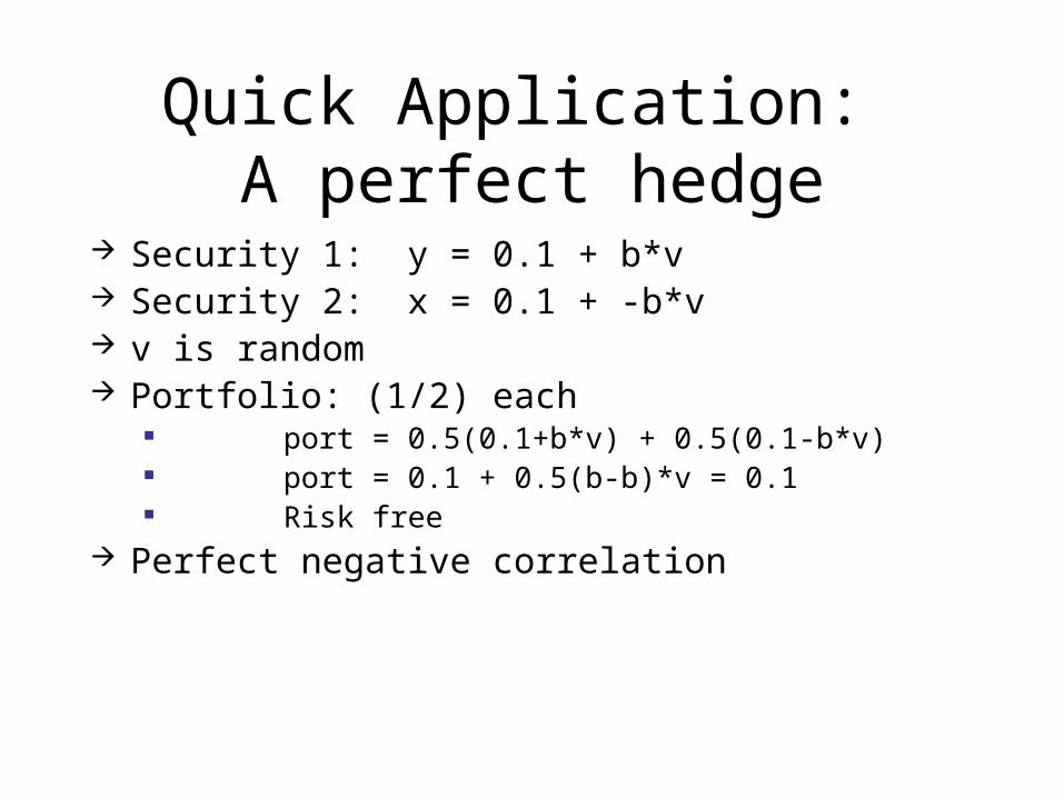
Security 1: y = 0.1 + b*v Security 2: x = 0.1 + -b*v v is random Portfolio: (1/2) each
port = 0.5(0.1+b*v) + 0.5(0.1-b*v) port = 0.1 + 0.5(b-b)*v = 0.1 Risk free
Perfect negative correlation
Summary: Portfolio Theory
A radically new approach to risk In the 1950’s
Two key points Diversification matters Worry about how an investment moves
with the rest of your portfolio Worry more about correlations than
standard deviations and variances

Goals
Portfolios and correlationsDiversifiable versus nondiversifiable riskCAPM and Beta
Capital asset pricing model Is the CAPM really useful?
Nondiversifiable Risk
Many equity returns are positively correlated
What does that mean to our new thoughts on risk?
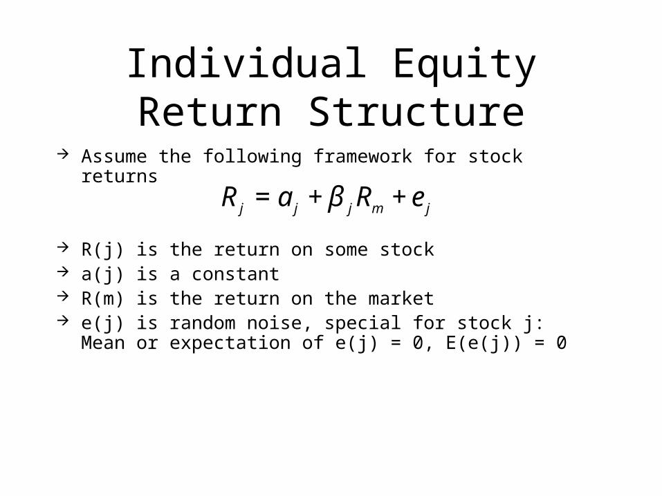
Individual Equity Return Structure
Assume the following framework for stock returns
R(j) is the return on some stock a(j) is a constant R(m) is the return on the market e(j) is random noise, special for stock j: Mean or expectation of
e(j) = 0, E(e(j)) = 0€
R j = a j + β jRm + e j
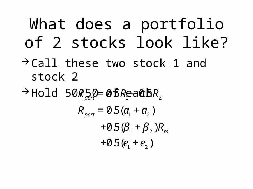
What does a portfolio of 2 stocks look like?
Call these two stock 1 and stock 2Hold 50/50 of each
€
Rport = 0.5R1 + 0.5R2
Rport = 0.5(a1 + a2 )
+0.5(β1 + β 2 )Rm+0.5(e1 + e2 )
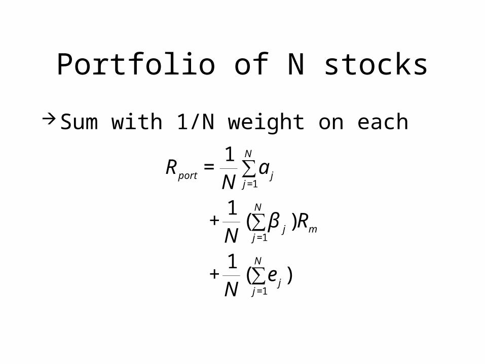
Portfolio of N stocks
Sum with 1/N weight on each
€
Rport =1N
a jj=1
N
∑
+1N
( β jj=1
N
∑ )Rm
+1N
( e jj=1
N
∑ )
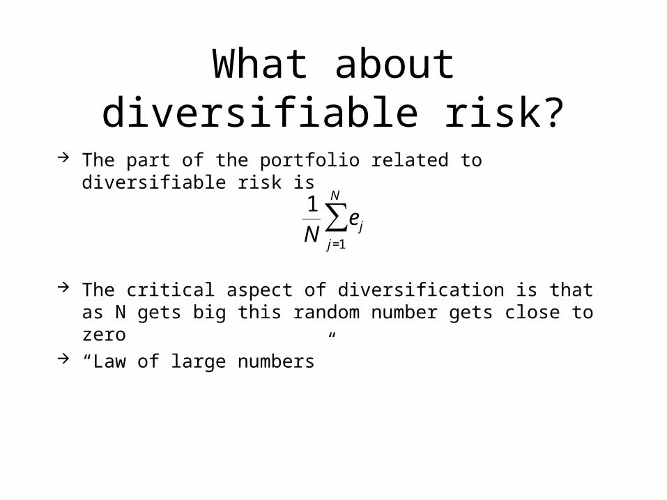
What about diversifiable risk?
The part of the portfolio related to diversifiable risk is
The critical aspect of diversification is that as N gets big this random number gets close to zero
“Law of large numbers”€
1N
ejj=1
N
∑

Risk Reduction
Number of Securities
Portfolio Risk(Variance or standard deviation)
Nondiversifiable Risk (systematic)
Diversifiable Risk (unsystematic)
Why?
This is a little like going to a casino, and playing roulette
You bet on red many, many timesKeep track of W/(W+L)As you play more and more this gets
very close to 0.5
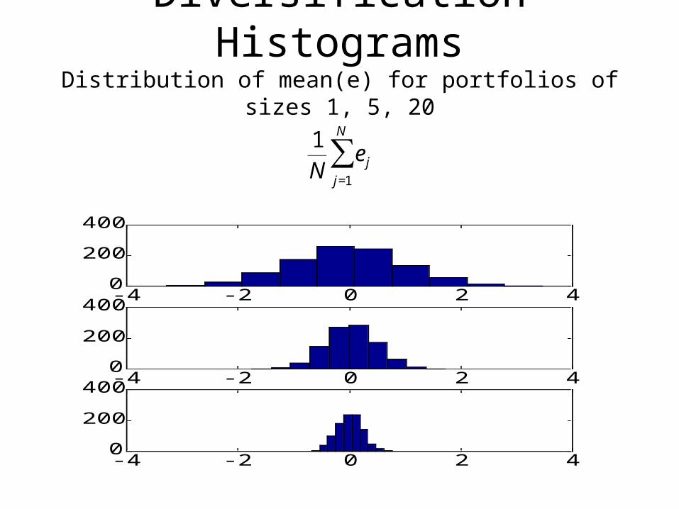
Diversification HistogramsDistribution of mean(e) for portfolios of sizes 1, 5, 20
-4 -2 0 2 40
200
400
-4 -2 0 2 40
200
400
-4 -2 0 2 40
200
400
€
1N
ejj=1
N
∑
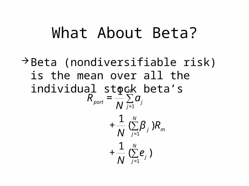
What About Beta?
Beta (nondiversifiable risk) is the mean over all the individual stock beta’s
€
Rport =1N
a jj=1
N
∑
+1N
( β jj=1
N
∑ )Rm
+1N
( e jj=1
N
∑ )
Key issue
For equities the diversifiable part of risk can be eliminated
All that remains is the part that moves with the market, or the nondiversifiable risk
This depends on beta ONLY
Java Example
See web example
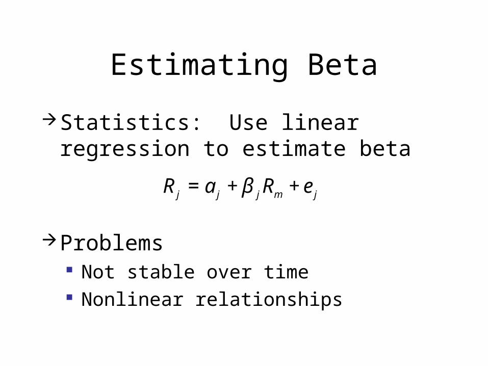
Estimating Beta
Statistics: Use linear regression to estimate beta
Problems Not stable over time Nonlinear relationships€
R j = a j + β jRm + e j

Goals
Portfolios and correlationsDiversifiable versus nondiversifiable riskCAPM and Beta
Capital asset pricing model Is the CAPM really useful?
Capital Asset Pricing Model (CAPM)
Risk depends on Beta alone If there is a payoff of higher return for
higher risk, then alpha, the expected return, depends on Beta only
In the CAPM world Beta is the key component of risk
What would happen in a non CAPM world?Malkiel’s experiment
Assume the risk measure that people care about is related to the total (nondiversifiable+diversifiable) risk
Stocks with higher e(j) variance pay higher returns
Build two stock portfolios High e(j) variance, Beta = 1 Low e(j) variance, Beta = 1
More on Malkiel’s Experiment
Since this is a nonCAPM world The first portfolio earns a higher return
However, the risk of the two portfolios is the same They have the same beta e(j) risk is diversified away
Investors will load up on high e(j) risk stocks This drives the price up, and expected returns will
fall on these stocks until they are equal to the others
Beta is Key
In the CAPM world: No reward for holding stocks with lots of
diversifiable risk Only beta matters as a measure of risk
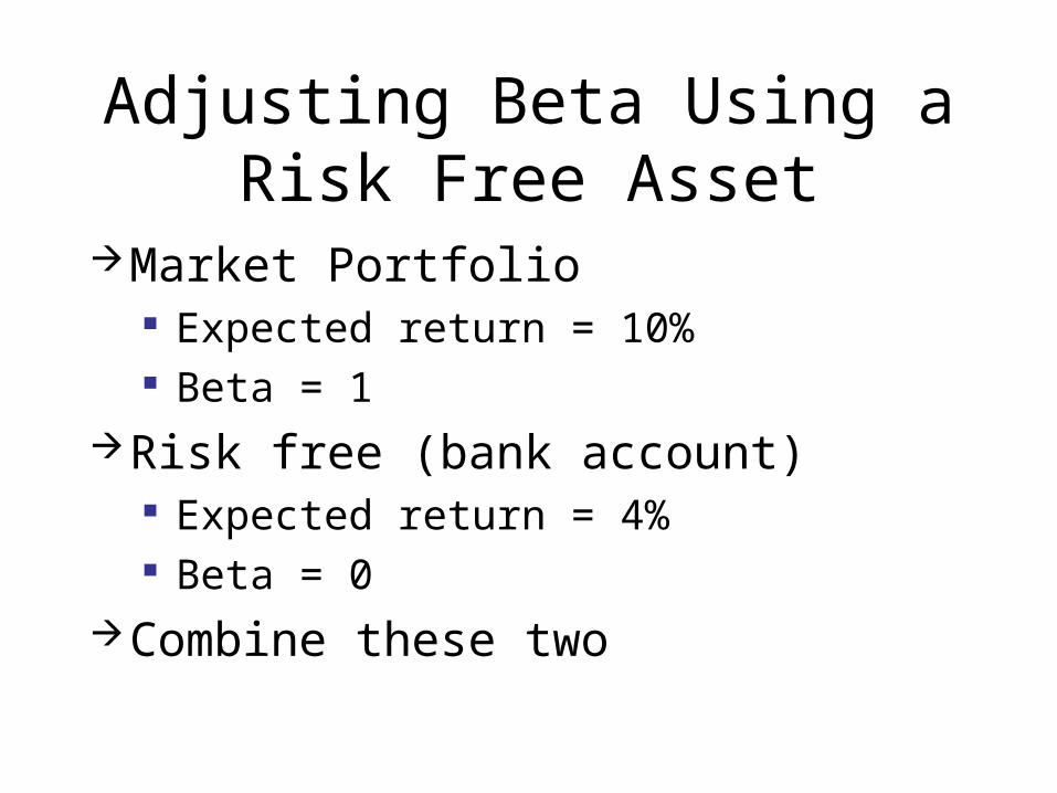
Adjusting Beta Using a Risk Free Asset
Market Portfolio Expected return = 10% Beta = 1
Risk free (bank account) Expected return = 4% Beta = 0
Combine these two
Combinations
All risk free Beta = 0, expected return = 4%
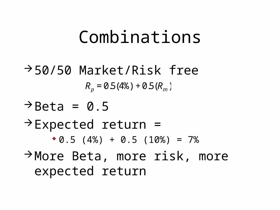
Combinations
50/50 Market/Risk free
Beta = 0.5Expected return =
0.5 (4%) + 0.5 (10%) = 7%
More Beta, more risk, more expected return
€
Rp = 0.5(4%)+ 0.5(Rm )
Fully Invested in Market
Easy Beta = 1 Expected return = 10%
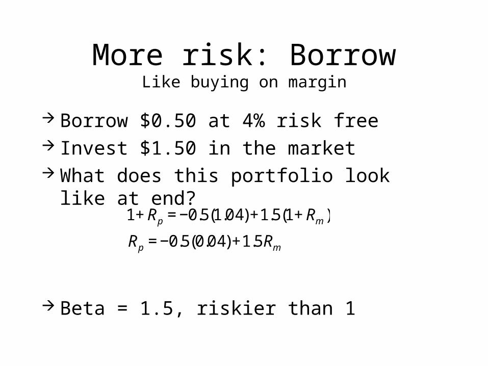
More risk: BorrowLike buying on margin
Borrow $0.50 at 4% risk free Invest $1.50 in the market What does this portfolio look like at end?
Beta = 1.5, riskier than 1
€
1+ Rp = −0.5(1.04)+1.5(1+ Rm )
Rp = −0.5(0.04)+1.5Rm
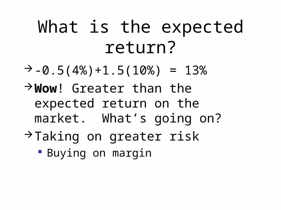
What is the expected return?
-0.5(4%)+1.5(10%) = 13%Wow! Greater than the expected return
on the market. What’s going on?Taking on greater risk
Buying on margin
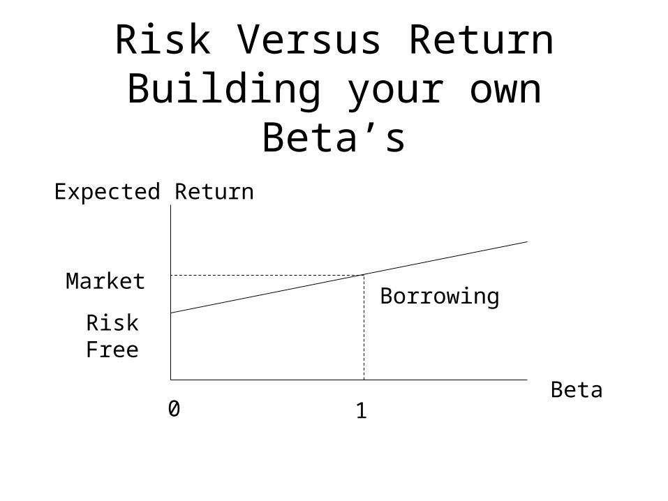
Risk Versus ReturnBuilding your own Beta’s
Beta
Expected Return
0
Risk Free
1
MarketBorrowing
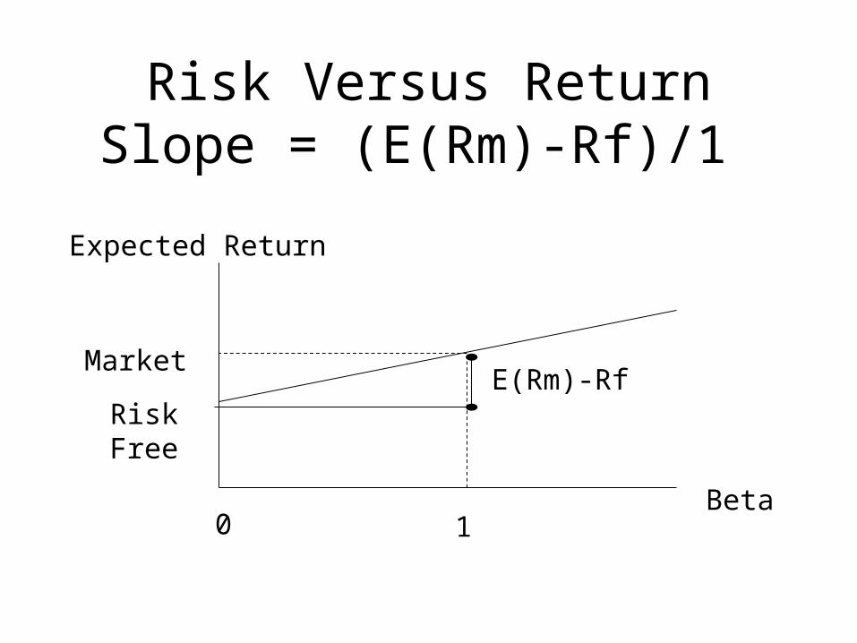
Risk Versus ReturnSlope = (E(Rm)-Rf)/1
Beta
Expected Return
0
Risk Free
1
MarketE(Rm)-Rf
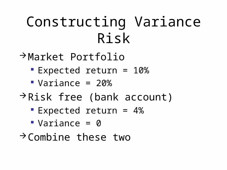
Constructing Variance Risk
Market Portfolio Expected return = 10% Variance = 20%
Risk free (bank account) Expected return = 4% Variance = 0
Combine these two
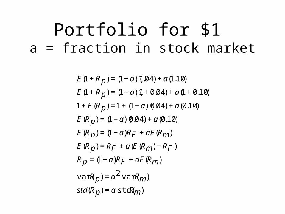
Portfolio for $1 a = fraction in stock market
€
E(1 + Rp) = (1 − a)(1.04) + a(1.10)
E(1 + Rp) = (1 − a)(1 + 0.04) + a(1 + 0.10)
1 + E(Rp) = 1 + (1 − a)(0.04) + a(0.10)
E(Rp) = (1 − a)(0.04) + a(0.10)
E(Rp) = (1 − a)RF + aE(Rm )
E(Rp) = RF + a(E(Rm ) − RF )
Rp = (1 − a)RF + aE(Rm )
var(Rp) = a2 var(Rm )
std (Rp) = a std(Rm )
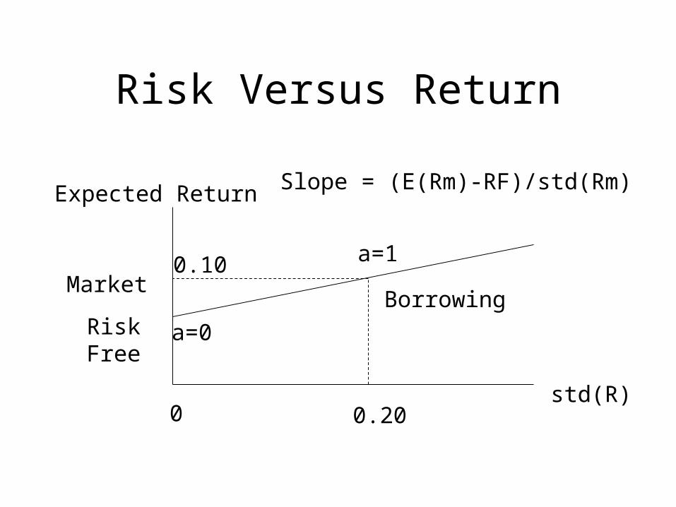
Risk Versus Return
std(R)
Expected Return
0
Risk Free
0.20
MarketBorrowing
a=1
a=0
0.10
Slope = (E(Rm)-RF)/std(Rm)
Returns and Borrowing
By borrowing more (leverage) can increase returns
Also, increase risk It is easy to be on the line (if you have
enough credit) Simply reporting returns alone is never
enough Would a return of 20% per year be amazing?
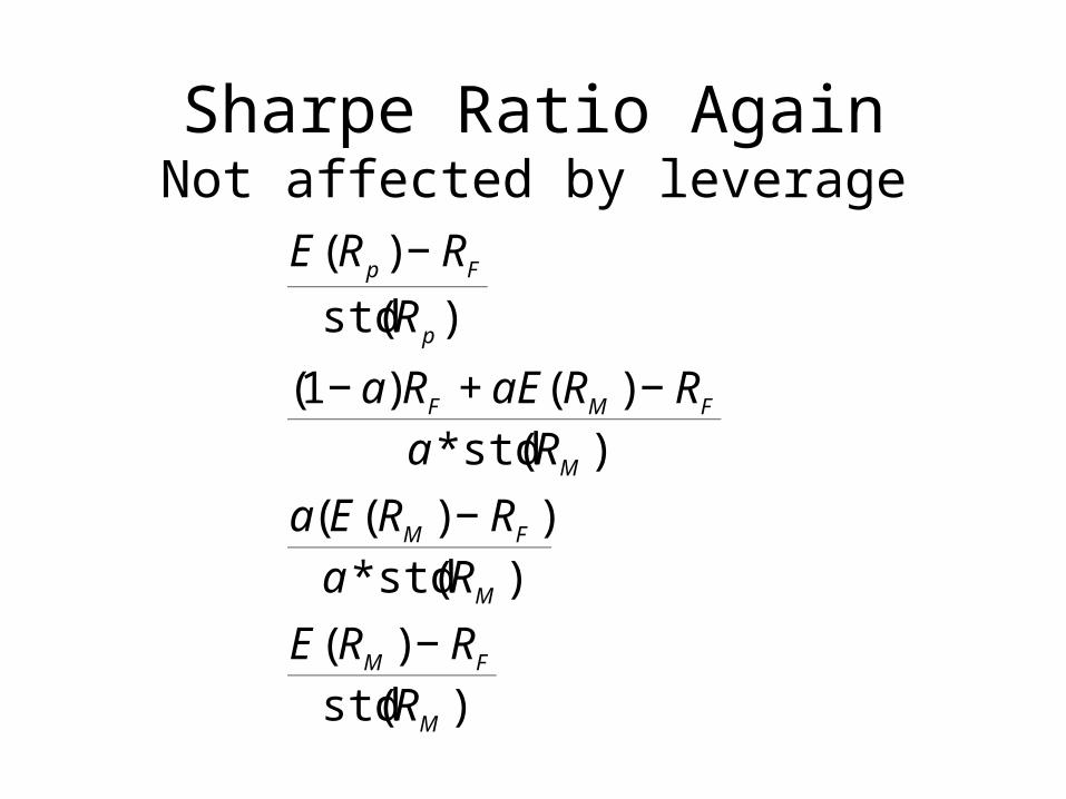
Sharpe Ratio AgainNot affected by leverage
€
E(Rp ) − RFstd(Rp )
(1− a)RF + aE(RM ) − RFa*std(RM )
a(E(RM ) − RF )a*std(RM )
E(RM ) − RFstd(RM )
CAPM: Two views
Simple risk measure, BetaPerfect CAPM world
Market equilibrium linking beta and expected returns
Perfect CAPM World
Beta (and Beta alone) is risk measureEveryone holds market portfolio and
some amount of risk free Individual stock returns and Beta are
linearly related
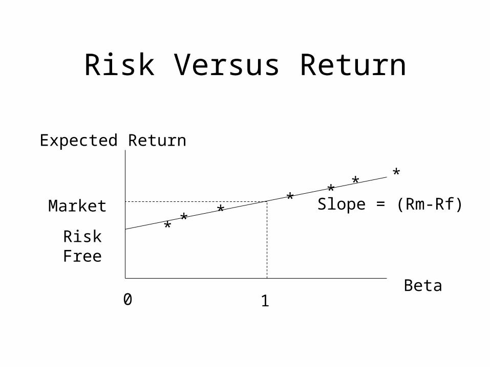
Risk Versus Return
Beta
Expected Return
0
Risk Free
1
Market*
***
*
**
Slope = (Rm-Rf)
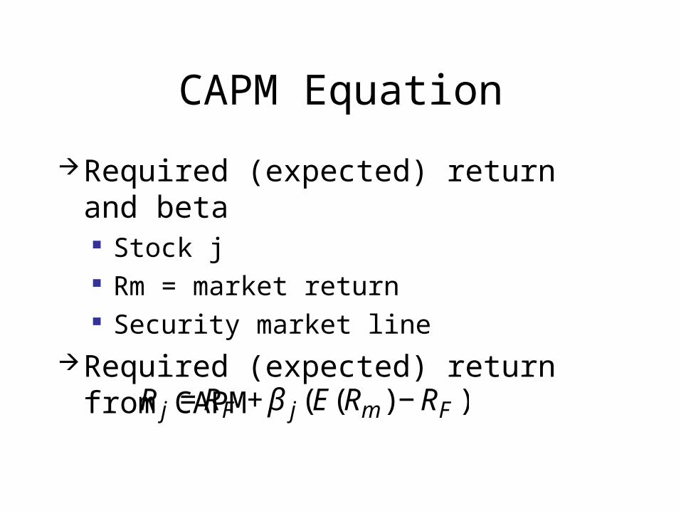
CAPM Equation
Required (expected) return and beta Stock j Rm = market return Security market line
Required (expected) return from CAPM
€
R j = RF + β j (E(Rm ) − RF )
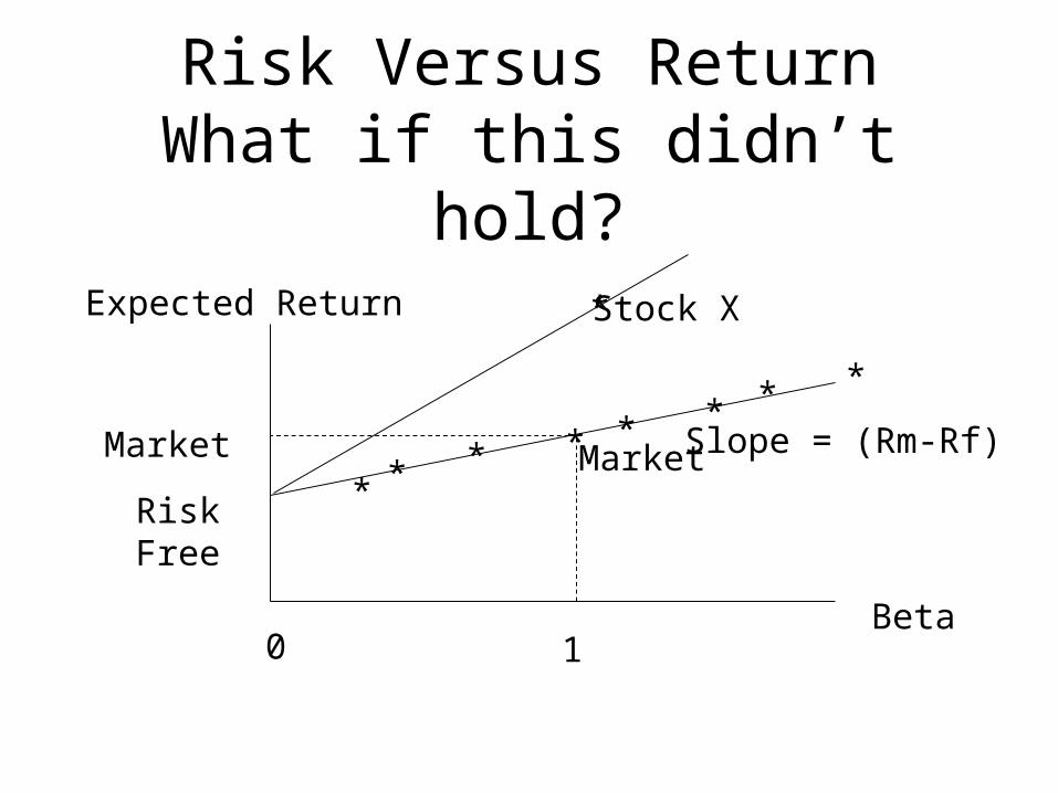
Risk Versus ReturnWhat if this didn’t hold?
Beta
Expected Return
0
Risk Free
1
Market*
***
*
**
Slope = (Rm-Rf)
*
* Market
Stock X
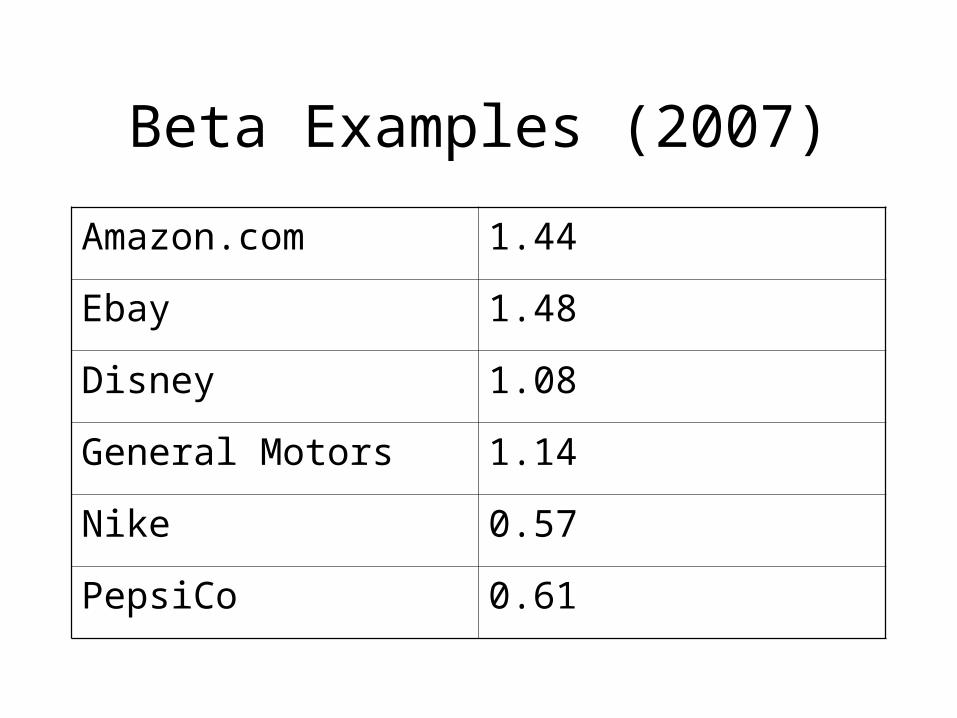
Beta Examples (2007)
Amazon.com 1.44
Ebay 1.48
Disney 1.08
General Motors 1.14
Nike 0.57
PepsiCo 0.61
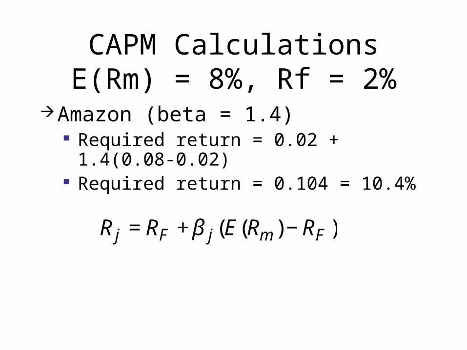
CAPM CalculationsE(Rm) = 8%, Rf = 2%
Amazon (beta = 1.4) Required return = 0.02 + 1.4(0.08-0.02) Required return = 0.104 = 10.4%
€
R j = RF + β j (E(Rm ) − RF )
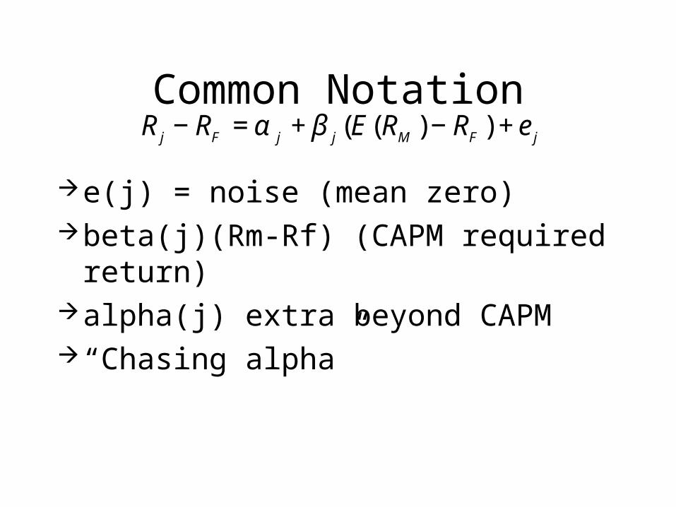
Common Notation
€
R j − RF = α j + β j (E(RM ) − RF ) + e j
e(j) = noise (mean zero)beta(j)(Rm-Rf) (CAPM required return)alpha(j) extra beyond CAPM “Chasing alpha”

Goals
Portfolios and correlationsDiversifiable versus nondiversifiable riskCAPM and Beta
Capital asset pricing model Is the CAPM really useful?
How well does the CAPM work?
Results: Fama and French Malkiel
Construct portfolios of stocksEstimate betasPlot beta versus expected returnNo relationship
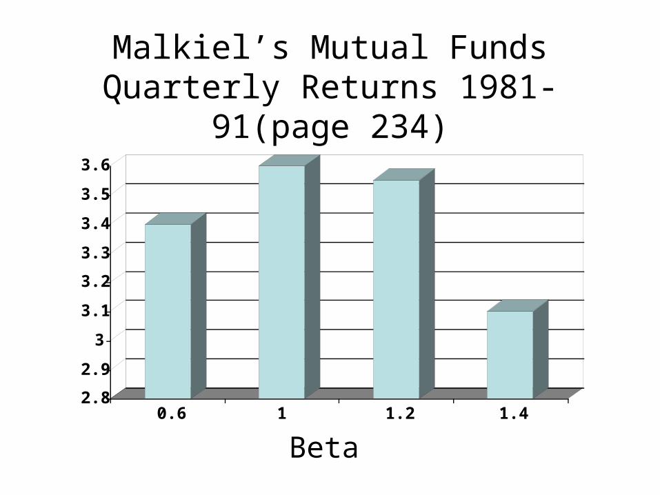
Malkiel’s Mutual FundsQuarterly Returns 1981-91(page
234)
2.8
2.9
3
3.1
3.2
3.3
3.4
3.5
3.6
0.6 1 1.2 1.4
Beta
Is Beta Dead?
Older research showed a weak relationship between beta and expected return
Recent evidence shows that there is probably no relationship
Premier model of asset pricingShould or do we still care?
Reasons to Still think about Beta
Diversification and portfolio theory is still important Beta is informative about how a security
moves with the market If the CAPM is not working, should try to
“beat it” Load up on low beta stocks Should be lower risk, and higher return
Problems with CAPM
Beta is very unstable over time Hard to estimate
Market inefficiencyDiversificationAttitudes toward risk Important side message
Look at other stuff
Goals
Portfolios and correlationsDiversifiable versus nondiversifiable riskCAPM and Beta
Capital asset pricing model Is the CAPM really useful?
Recommended