Download pdf - FEA Slope - Theoretical Manual - terrainsoft.net Slope - Theoretical Manual.pdf · ... A Finite Element Analysis of Slopes THEORETIC MANUAL. ... from system algebraic solution, and

Dr. Eng. Angelo S. Rabuffetti - © 2014

Studio Terrain – Milano – Italy

FE

A –

Slo

pe –

A F

inite

Ele

men

t Ana

lysi

s of

Slo

pes

THEORETIC MANUAL


Studio Terrain – Milano – Italy Page 2 of 2

SUMMARY SUMMARY ..........................................................................................................................2 ABOUT THE METHOD........................................................................................................3 1 – THE FINITE ELEMENTS METHOD...............................................................................5

1.1 – GENERALS.............................................................................................................5 1.2 – F.E. ALGORITHM AND NUMERICAL SOLUTION..................................................5

1.2.1 – STIFFNESS MATRIX OF A SINGLE ELEMENT ..............................................9 1.2.2 – THE SHAPE FUNCTIONS..............................................................................11 1.2.2.1 – QUADRILATERAL EIGHT-NODED ELEMENTS SHAPE FUNCTIONS......12 1.2.3 – DERIVATIVES RESPECT TO GLOBAL CO-ORDINATES (x, y)....................12 1.2.4 – NUMERICAL INTEGRATIONS FOR QUADRILATERAL ELEMENTS ...........13 1.2.5 – TRIANGULAR ELEMENTS ............................................................................13

1.3 – SO, HOW A F.E. ALGORITHM WORKS?.............................................................13 2 – GEOTECHNICAL ANALYSIS AND MATERIAL’S NON-LINEARITY...........................15

2.1 – STATES OF STRESS ...........................................................................................17 2.2 - THE MOHR-COULOMB FAILURE CRITERION....................................................17

2.2.1 – THE HOEK-BROWN MODEL FOR ROCKS...................................................19 2.3 – DRAINED AND UNDRAINED CONDITIONS........................................................21

2.3.1 – POSSIBLE GROUNDWATER OPTIONS .......................................................22 2.4 - VISCO-PLASTICITY ..............................................................................................23 2.5 – “ASSOCIATED” AND “NON ASSOCIATED” PLASTIC FLOW. DILATANCY........26 2.6 – SEISMIC CONDITIONS ........................................................................................27 2.7 – NON LINEARITY...................................................................................................28

3 – SLOPE STABILITY AND GEOTECHNICAL PROBLEMS ...........................................30

3.1 – DIFFUSION MECHANISM ....................................................................................30 3.2 – THE GEOTECHNICAL “SAFETY FACTOR” OF THE SLOPE..............................31

Bibliography .......................................................................................................................33



ABOUT THE METHOD FEA – Slope is a new program for the slope stability analysis based upon a robust Finite element (FEM) algorythm. The slope is modeled by use of eight-noded finite elements, defined by proper geometrical and geotechnical characteristics. Soil properties are defined in terms of cohesion, angle of internal friction, dilatancy, Poisson’s coefficient and Young’s modulus. These parameters can be easily obtained by: - in situ – tests ot by lab tests for the Mohr – Coulomb model (soils) - by correlations with proper parameters for the Hoek-Brown model (rocks)

The geotechnical failure model entails a failure function of non-associate type, developed in a visco-plastic behaviour theory. The failure analysis is run after the Mohr-Coulomb criterion and results in: - a “safety coefficient” against the slope collapse - the expected geometry of failil soil mass, allowing a definition of the sliding surface - an incremental forecast of failure mode, allowing a qualitative / quantitative

comparision via installation of geotechnical instrumentation - a failure tomography after the Mohr – Coulomb criterion, with identification of the

soil masses in verge of sliding sinche the very initial phase of process. Geometry of the problem is defined by input of points, single quadrilateral elements and /or full meshes od finite elements. The groundwater occurrence controls the establishment of total / effective soil stresses to be considered in each perticular solution. The seismic analysis is run by evaluating horizontal as well as vertical acceleration seismic fields, also concurrent, with vertical component either in upward or downward direction. In such a way, most recent european building code’s statements are allowed for. FEA – Slope implements an iterative multi – stage algorythm: In a premininary phase, the slope is analyzed in “initial” conditions, i. e. taking into account the mere data directly proceedeing from on site and laboratory tests. “Characteristic” values of soil strength parameters are introduced, without application of reduction factors. In the followings, the soil resistance parameters are decreased by enforcement of reduction factors (after the Strength Reduction Factor method – SRF), gradually increasing, until the slope finally fails because of poorness of actual reduced parameters. The collapse of a great number of elements results in development of a sliding surface and the general slope failure. Whenever a single soil element fails because of lack or resistance, the exceeding part of stress that cannot be resisted is re-sddressed along the element’s boundaries, burdening the neighboring elements. These elements, in turn, can resist overload or undergo failure, stating a new re-arrangement. At each further element’s collapse, the solving FEM system



is refreshed and a new solution is run in an iteraive manner, until some convergence is reached or not. If the convergence criterion is meet, the slope is considered as stable for the given geometry and current soil parameters (i.e. the shear parameters divided by the current reduction factor). The next step is to increase the reducing factor SRF affecting the shear resistance (i. e. the cohesion and the tangent of friction angle) and run a new FE analysis. Slope is defined as failed when, after a congruous number of algebraic iterations of system solving because of ceaseless stress’ re-distributions (suggested al least 500 iterations) calculations don’t converge, meaning an endless re-distribution of exceeding forces. The last reduction factor for shear prameters before failure can be taken as “safety factor” of the slope. More details about FEM re-distribution work can be found also in Rabuffetti (2012, 2013).



1 – THE FINITE ELEMENTS METHOD 1.1 – GENERALS

The Finite Elements Method (FEM) is a technique of resolution of partial differential equations by discretizatioon of such equations in their spatial dimensions. Discretization is carried out over small arbitrarily-defined regions (finite elements) carrying significant characteristic for the problem to be solved. In the solution a global algebraic matrix is built, in which each equation is referred to a speficic node of the system, featuring geometrical and mechanical soil properties, as well as external applied forces. Equations are solved resulting in a series of significant quantities for each node. In most elaborations these quantities are the nodal displacements. The global matrix results from the superpositions of actions and effects of actions coming from the previously defined discrete elements. The solution of the algebraic system allows the definition of unknowns in the whole space under consideration. Nodal values come directly from system algebraic solution, and points inside each element are the defined also. The relationship joining the values computed for each node on the boundary with points inside the finite elements are the shape funcions of the element. 1.2 – F.E. ALGORITHM AND NUMERICAL SOLUTION

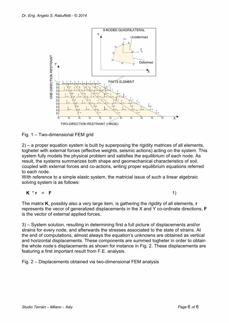
Once the soil profile is defined as a grid by use of elements and relevant nodes, the algorithm is implemented as follows: 1 – development of some relationship able to epitomize in each node any significant characteristics, as typically rigidity, mass, weight (in soil mechanics, the rigidity matrix). These relationships, systematically obtained by numerical integrations, translate in linear equations the derivatives bearing the stress/strain relationships. An example of a FEM mesh, in which elements and relevant nodes and freedoms in the co-ordinate directions X and Y are pointed out, is shown in the following Fig. 1.



Fig. 1 – Two-dimensional FEM grid 2) – a proper equation system is built by superposing the rigidity matrices of all elements, togheter with external forces (effective weights, seismic actions) acting on the system. This system fully models the physical problem and satisfies the equilibrium of each node. As result, the systems summarizes both shape and geomechanical characteristics of soil, coupled with external forces and co-actions, writing proper equilibrium equations referred to each node. With reference to a simple elastc system, the matricial issue of such a linear algebraic solving system is as follows: K * r = F 1)

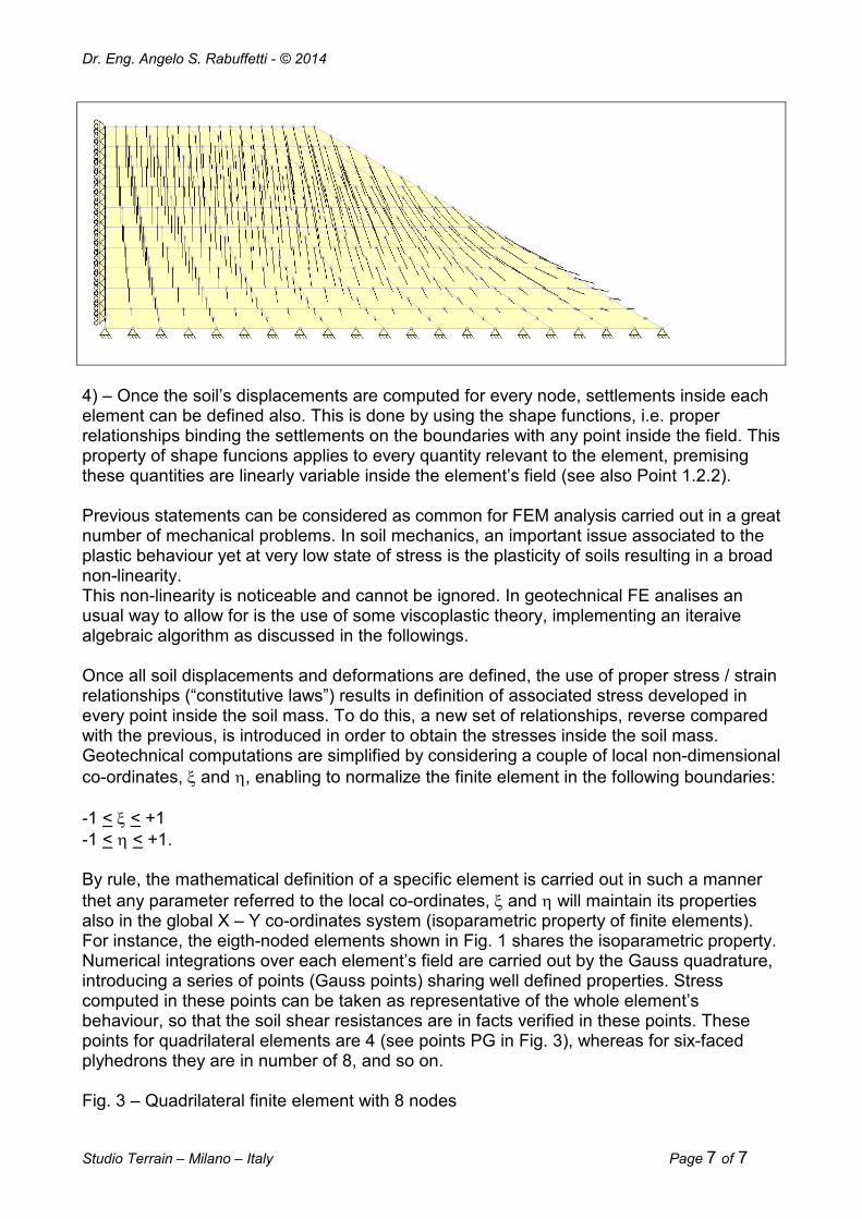
The matrix K, possibly also a very large item, is gathering the rigidity of all elements, r represents the vecor of generalized displacements in the X and Y co-ordinate directions, F is the vector of external applied forces. 3) – System solution, resulting in determining first a full picture of displacements and/or strains for every node, and afterwards the stresses associated to the state of strains. At the end of computations, almost always the equation’s unknowns are obtained as vertical and horizontal displacements. These components are summed togheter in order to obtain the whole node’s displacements as shown for instance in Fig. 2. These displacements are featuring a first important result from F.E. analysis. Fig. 2 – Displacements obtained via two-dimensional FEM analysis



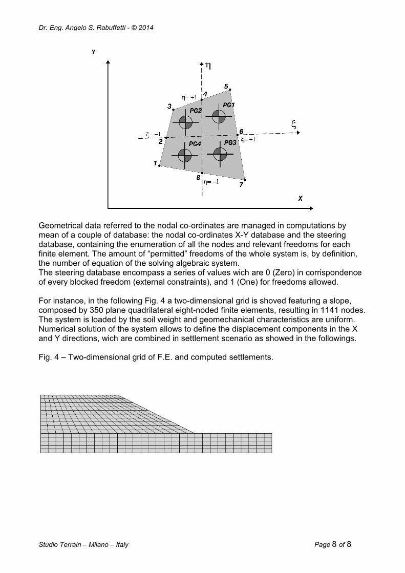
4) – Once the soil’s displacements are computed for every node, settlements inside each element can be defined also. This is done by using the shape functions, i.e. proper relationships binding the settlements on the boundaries with any point inside the field. This property of shape funcions applies to every quantity relevant to the element, premising these quantities are linearly variable inside the element’s field (see also Point 1.2.2). Previous statements can be considered as common for FEM analysis carried out in a great number of mechanical problems. In soil mechanics, an important issue associated to the plastic behaviour yet at very low state of stress is the plasticity of soils resulting in a broad non-linearity. This non-linearity is noticeable and cannot be ignored. In geotechnical FE analises an usual way to allow for is the use of some viscoplastic theory, implementing an iteraive algebraic algorithm as discussed in the followings. Once all soil displacements and deformations are defined, the use of proper stress / strain relationships (“constitutive laws”) results in definition of associated stress developed in every point inside the soil mass. To do this, a new set of relationships, reverse compared with the previous, is introduced in order to obtain the stresses inside the soil mass. Geotechnical computations are simplified by considering a couple of local non-dimensional co-ordinates, ξ and η, enabling to normalize the finite element in the following boundaries: -1 < ξ < +1 -1 < η < +1. By rule, the mathematical definition of a specific element is carried out in such a manner thet any parameter referred to the local co-ordinates, ξ and η will maintain its properties also in the global X – Y co-ordinates system (isoparametric property of finite elements). For instance, the eigth-noded elements shown in Fig. 1 shares the isoparametric property. Numerical integrations over each element’s field are carried out by the Gauss quadrature, introducing a series of points (Gauss points) sharing well defined properties. Stress computed in these points can be taken as representative of the whole element’s behaviour, so that the soil shear resistances are in facts verified in these points. These points for quadrilateral elements are 4 (see points PG in Fig. 3), whereas for six-faced plyhedrons they are in number of 8, and so on. Fig. 3 – Quadrilateral finite element with 8 nodes



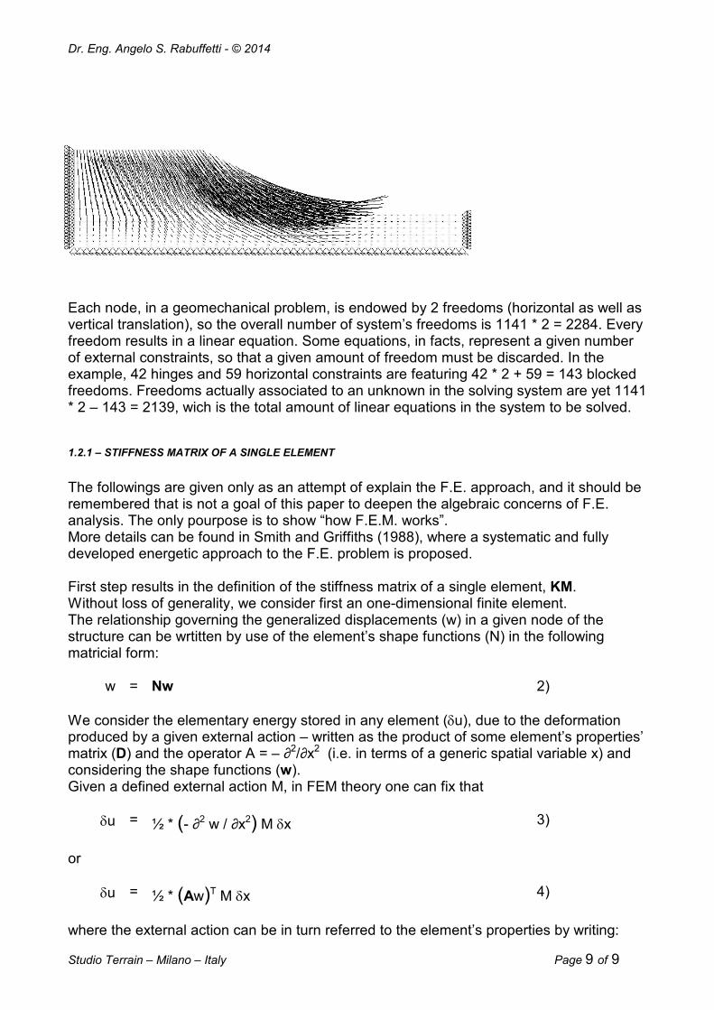
Geometrical data referred to the nodal co-ordinates are managed in computations by mean of a couple of database: the nodal co-ordinates X-Y database and the steering database, containing the enumeration of all the nodes and relevant freedoms for each finite element. The amount of “permitted” freedoms of the whole system is, by definition, the number of equation of the solving algebraic system. The steering database encompass a series of values wich are 0 (Zero) in corrispondence of every blocked freedom (external constraints), and 1 (One) for freedoms allowed. For instance, in the following Fig. 4 a two-dimensional grid is shoved featuring a slope, composed by 350 plane quadrilateral eight-noded finite elements, resulting in 1141 nodes. The system is loaded by the soil weight and geomechanical characteristics are uniform. Numerical solution of the system allows to define the displacement components in the X and Y directions, wich are combined in settlement scenario as showed in the followings. Fig. 4 – Two-dimensional grid of F.E. and computed settlements.



Each node, in a geomechanical problem, is endowed by 2 freedoms (horizontal as well as vertical translation), so the overall number of system’s freedoms is 1141 * 2 = 2284. Every freedom results in a linear equation. Some equations, in facts, represent a given number of external constraints, so that a given amount of freedom must be discarded. In the example, 42 hinges and 59 horizontal constraints are featuring 42 * 2 + 59 = 143 blocked freedoms. Freedoms actually associated to an unknown in the solving system are yet 1141 * 2 – 143 = 2139, wich is the total amount of linear equations in the system to be solved.

1.2.1 – STIFFNESS MATRIX OF A SINGLE ELEMENT

The followings are given only as an attempt of explain the F.E. approach, and it should be remembered that is not a goal of this paper to deepen the algebraic concerns of F.E. analysis. The only pourpose is to show “how F.E.M. works”. More details can be found in Smith and Griffiths (1988), where a systematic and fully developed energetic approach to the F.E. problem is proposed. First step results in the definition of the stiffness matrix of a single element, KM. Without loss of generality, we consider first an one-dimensional finite element. The relationship governing the generalized displacements (w) in a given node of the structure can be wrtitten by use of the element’s shape functions (N) in the following matricial form:

w = Nw 2) We consider the elementary energy stored in any element (δu), due to the deformation produced by a given external action – written as the product of some element’s properties’ matrix (D) and the operator A = – ∂2/∂x2 (i.e. in terms of a generic spatial variable x) and considering the shape functions (w). Given a defined external action M, in FEM theory one can fix that

δu = ½ * (- ∂2 w / ∂x2) M δx 3)

or

δu = ½ * (Aw)T M δx 4)

where the external action can be in turn referred to the element’s properties by writing:



M = D A w 5)

One can then infer that

δu = ½ * (ANw)T DANw δx

= ½ * wT (AN)T DANw δx 6)

and, by integrating over the whole finite element over x,

L U = ½ * wT (AN)T DAN w dx 7)

∫ o

The syntetic F.E. notation for AN is usually referred as B, whereas wT is substantially indipendent from x, so that one can write

L U = ½ * wT BT D B dx w 8)

∫ o Remembering the actual energetic mean of U (“kinetic” energy due to an external action M resulting a deformation in terms of w), the F.E. theory considers the following general relationship:

L L BT D B dx w = q NT dx 9)

∫ o ∫ o where q represents the elementary external action. From a statical standpoint, one can write also the following relationship:

L KM w = q NT dx 10)

∫ o where KM is defined as stiffness matrix of the element. From the above relationships, one can finally infer a definition very useful in order to write the stiffness’ matrix of a certain element:

L KM = BT D B dx 11)

∫ o The above relationships are relevant to an one-dimensional element. In the two-dimensional plan, the integration of the deformational energy of an element, considering an unitary thickness, is carried out in two-dimensions as follows:



L U = ½ * σσσσT εεεε dx dy

∫∫ o L = ½ * rT (AN)T D (AN) dx dy r ∫∫ o L = ½ * rT BT D B dx dy r 7.1) ∫∫ o

where r carries the same significance as w in the liear case (shape functions), whilst operators A and D are defined in a plan element as follows: ∂/∂x 0 A = 0 ∂/∂y { ∂/∂y ∂/∂x } 1 ν 0 D = E / (1-ν2) ν 1 0 [ 0 0 (1-ν)/2

] and further: N1 N2 N3 N4 0 0 0 0 N = [ 0 0 0 0 N1 N2 N3 N4 ] As for 8), 9) and 10), in the case of a plan finite element we have in turn:

KM = BT D B dx dy 12)

∫∫ All terms for the two-dimensional case are more complex than for a linear element, but the common algebraic form is evident. Assemmbly of the solving system 1) is carried out by inserting all stiffness’ matrices of single elements 12) inside the “global stiffness matrix” of the sistem, usually defined as K.

1.2.2 – THE SHAPE FUNCTIONS

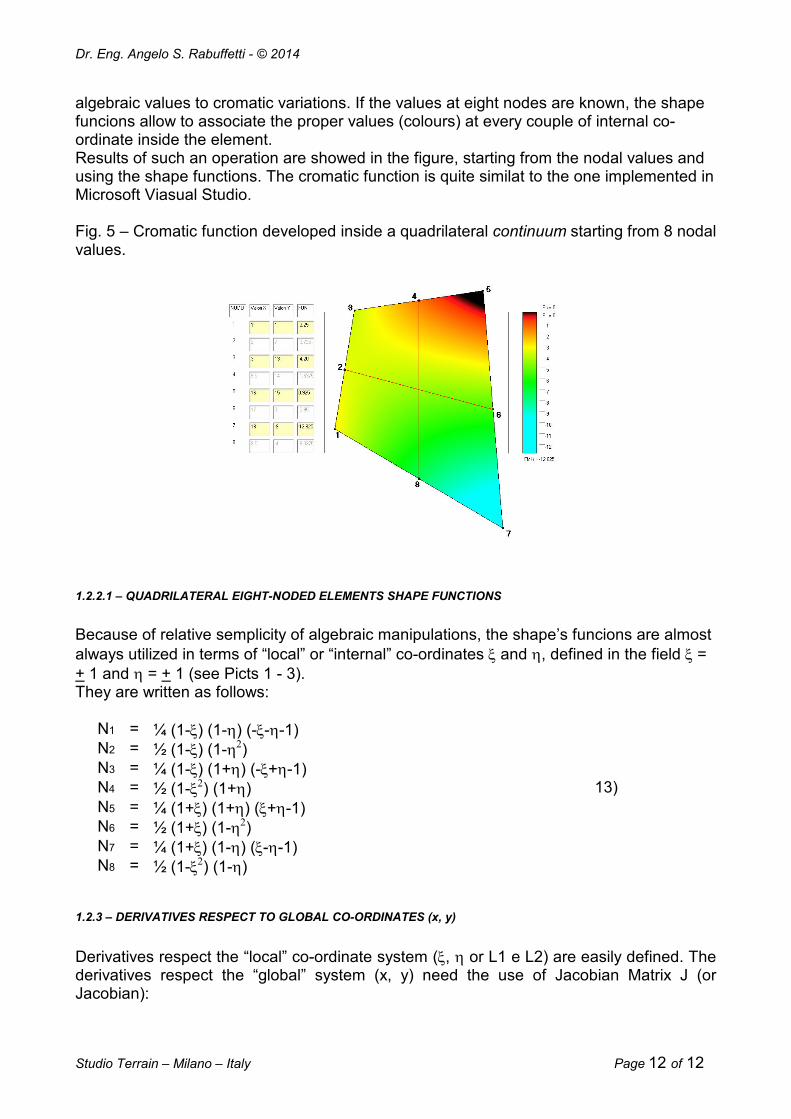
After the FEM system is solved for the unknown displacements in the nodes of the grid, the amount of correspondent displacements can be determined inside the continuum represented by the element, by mean of the shape functions. The FEA Slope’s shape functions are implemented according to Smith & Griffiths (1988) and Zienkiewicz & Taylor (1989). Derivatives, implemented by the A operator as previously mentionned, were consequently obtained. The 8-noded quadrilateral finite elements implement very effective shape functions for geotechnical solutions. As a simple exemplum of use of such functions, in the Fig. 5 the coverage of a cromatic function inside an element is showed. A given funcion is considered, able to couple



algebraic values to cromatic variations. If the values at eight nodes are known, the shape funcions allow to associate the proper values (colours) at every couple of internal co-ordinate inside the element. Results of such an operation are showed in the figure, starting from the nodal values and using the shape functions. The cromatic function is quite similat to the one implemented in Microsoft Viasual Studio. Fig. 5 – Cromatic function developed inside a quadrilateral continuum starting from 8 nodal values.

1.2.2.1 – QUADRILATERAL EIGHT-NODED ELEMENTS SHAPE FUNCTIONS

Because of relative semplicity of algebraic manipulations, the shape’s funcions are almost always utilized in terms of “local” or “internal” co-ordinates ξ and η, defined in the field ξ = + 1 and η = + 1 (see Picts 1 - 3). They are written as follows:

N1 = ¼ (1-ξ) (1-η) (-ξ-η-1) N2 = ½ (1-ξ) (1-η2) N3 = ¼ (1-ξ) (1+η) (-ξ+η-1) N4 = ½ (1-ξ2) (1+η) 13) N5 = ¼ (1+ξ) (1+η) (ξ+η-1) N6 = ½ (1+ξ) (1-η2) N7 = ¼ (1+ξ) (1-η) (ξ-η-1) N8 = ½ (1-ξ2) (1-η)

1.2.3 – DERIVATIVES RESPECT TO GLOBAL CO-ORDINATES (x, y)

Derivatives respect the “local” co-ordinate system (ξ, η or L1 e L2) are easily defined. The derivatives respect the “global” system (x, y) need the use of Jacobian Matrix J (or Jacobian):



∂ /∂ξ ∂ /∂x = J 14) { ∂ /∂η

}

{ ∂ /∂y

}

or:

∂ /∂x ∂ /∂ξ = J -1 15) { ∂ /∂y

}

{∂ /∂η

}

The determinant of the Jacobian Matrix, det │J│, must be computed in order to solve some integrals of the type:

1 1 dx dy = det │J│ dξ dη 16) ∫∫ ∫

-1 ∫

-1 It should be pointed out that the Jacobian becomes undetermined in case of concave polygons (quadrilaterals), which must be avoided.

1.2.4 – NUMERICAL INTEGRATIONS FOR QUADRILATERAL ELEMENTS

In facts, equations 16) are handled using the Gaussian quadrature over quadrilateral areas, as follows:

1 1 n n

f (ξ, η) dξ dη ≈ Σ Σ wi wj f(ξi, ηj) 17) ∫ -1

∫ -1 i=1 j=1

where wi and wj are “ponderal” cohefficients and ξi, ηj are co-ordinates inside the elements relevant to the Gauss’ quadrature points, or Gauss’ points. In the case under observation, we consider 2 Gauss’ point in vertical direction and 2 in horizontal (see Pict. 3), in such a manner that ξi ηj = + 1/ √3 when the integration field is +1. The approximate equality in 17) is exact for cubic functions where n = 2.

1.2.5 – TRIANGULAR ELEMENTS

FEA Slope uses triangular elements derived as limit situation for use of quadrilateral in which two adjacent sides are aligned. In such a manner the velocity in computation is not affected by building different solutions. 1.3 – SO, HOW A F.E. ALGORITHM WORKS?

At this stage, we can draw a plot of a “rigid” or “elastic” FEM solution. The mean of this will be clear in the subsequent chapter. In the following Pict. 6, the block diagram for a



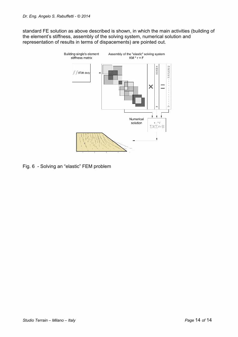
standard FE solution as above described is shown, in which the main activities (building of the element’s stiffness, assembly of the solving system, numerical solution and representation of results in terms of dispacements) are pointed out.

Fig. 6 - Solving an “elastic” FEM problem



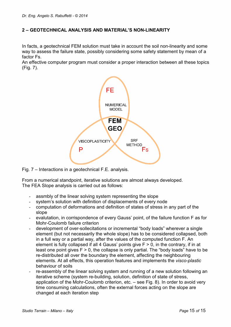
2 – GEOTECHNICAL ANALYSIS AND MATERIAL’S NON-LINEARITY In facts, a geotechnical FEM solution must take in account the soil non-linearity and some way to assess the failure state, possibly considering some safety statement by mean of a factor Fs. An effective computer program must consider a proper interaction between all these topics (Fig. 7).

Fig. 7 – Interactions in a geotechnical F.E. analysis. From a numerical standpoint, iterative solutions are almost always developed. The FEA Slope analysis is carried out as follows: - assmbly of the linear solving system representing the slope - system’s solution with definition of displacements of every node - computation of deformations and definition of states of stress in any part of the

slope - evalutation, in corrispondence of every Gauss’ point, of the failure function F as for

Mohr-Coulomb failure criterion - development of over-sollecitations or incremental “body loads” wherever a single

element (but not necessarily the whole slope) has to be considered collapsed, both in a full way or a partial way, after the values of the computed function F. An element is fully collapsed if all 4 Gauss’ points give F > 0, in the contrary, if in at least one point gives F > 0, the collapse is only partial. The “body loads” have to be re-distributed all over the boundary the element, affecting the neighbouring elements. At all effects, this operation features and implements the visco-plastic behaviour of soils

- re-assembly of the linear solving system and running of a new solution following an iterative scheme (system re-building, solution, definition of state of stress, application of the Mohr-Coulomb criterion, etc. – see Fig. 8). In order to avoid very time consuming calculations, often the external forces acting on the slope are changed at each iteration step



- evaluation of deformations with reference of the previous ones, with reference to the following convergence rule: - if the difference between actual and previous displacements in adequately small, the system is considered converging, and the slope stable, so the analisys is stopped - if the difference does not satisfy the convergence, a new iteration of calculation is performed

- in presence of an amount of iterations exceeding a pre-determined large number (e. g. 500 iterations), without convergence, the slope is considered as collapsed.

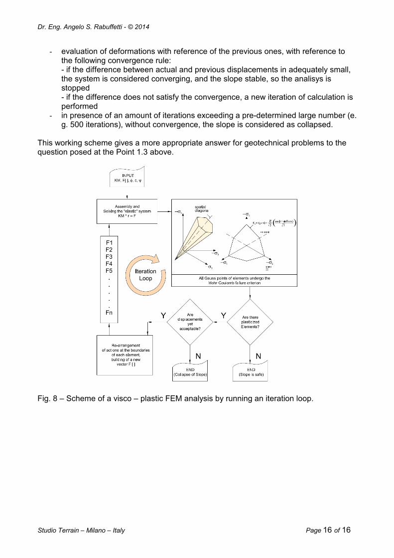
This working scheme gives a more appropriate answer for geotechnical problems to the question posed at the Point 1.3 above.

Fig. 8 – Scheme of a visco – plastic FEM analysis by running an iteration loop.



2.1 – STATES OF STRESS

As a general rule, the stress representation of a point inside a loaded body can be summarized as a Cartesian tensor, as follows: { σx σy σz τxy τyz τzx } 18) which in turn equals the main orthogonal principal stress tensor: { σ1 σ2 σ3 } 19) whose orientation in the space is generally unknown. In F.E. computations the following stress invariants are preferred: s = 1/√3 ( σx + σy + σz) 20.1) t = 1/√3 [ (σx-σy )2 + (σy-σz )2 + (σz-σx )2 + 6 τ2

xy + 6 τ2yz + 6 τ2

zx]1/2 20.2) θ = 1/3 arc sin (-3 √6 J3 / t3) 20.3) where: J3 = σx σy σz - σx τ2

yz - σy τ2zx - σz τ2

xy + 2 τxy τyz τzx σx = (2 σx - σy - σz) / 3 , etc. In physical terms, a given point P (σx, σy, σz) can be described in terms of distance (s) between its plane π from the origin, distance (t) from the spatial diagonal, and the Lode angle (θ) representing the angular position of the same point on π plane (see Fig. 9). Finally, a more effective representation by exploitation of the following terms: σm = s/√3 σ = t/√(3/2) Leading to the following relationships between principal stresses and invariants: σ1 = σm + √(2/3) σ sin (θ - 2 π /3) 21.1) σ2 = σm + √(2/3) σ sin (θ ) 21.2) σ3 = σm + √(2/3) σ sin (θ + 2 π /3) 21.3) For each F.E. solution, FEA Slope computes principal stresses inside each finite element to detect occurrence of failure. 2.2 - THE MOHR-COULOMB FAILURE CRITERION



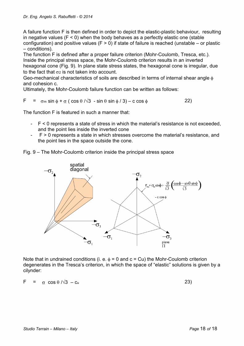
A failure function F is then defined in order to depict the elastic-plastic behaviour, resulting in negative values (F < 0) when the body behaves as a perfectly elastic one (stable configuration) and positive values (F > 0) if state of failure is reached (unstable – or plastic – conditions). The function F is defined after a proper failure criterion (Mohr-Coulomb, Tresca, etc.). Inside the principal stress space, the Mohr-Coulomb criterion results in an inverted hexagonal cone (Fig. 9). In plane state stress states, the hexagonal cone is irregular, due to the fact that σ2 is not taken into account. Geo-mechanical characteristics of soils are described in terms of internal shear angle φ and cohesion c. Ultimately, the Mohr-Coulomb failure function can be written as follows: F = σm sin φ + σ ( cos θ /√3 - sin θ sin φ / 3) – c cos φ 22) The function F is featured in such a manner that:

- F < 0 represents a state of stress in which the material’s resistance is not exceeded, and the point lies inside the inverted cone

- F > 0 represents a state in which stresses overcome the material’s resistance, and the point lies in the space outside the cone.

Fig. 9 – The Mohr-Coulomb criterion inside the principal stress space

Note that in undrained conditions (i. e. φ = 0 and c = Cu) the Mohr-Coulomb criterion degenerates in the Tresca’s criterion, in which the space of “elastic” solutions is given by a cilynder: F = σ cos θ /√3 – cu 23)



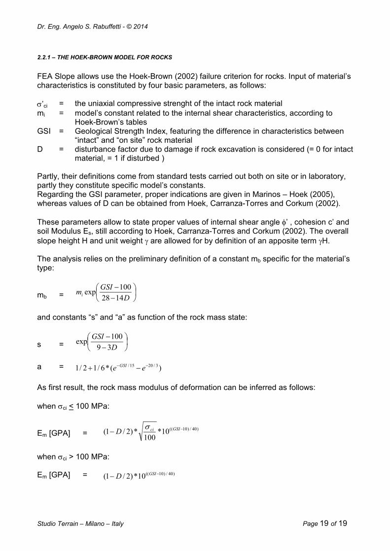
2.2.1 – THE HOEK-BROWN MODEL FOR ROCKS

FEA Slope allows use the Hoek-Brown (2002) failure criterion for rocks. Input of material’s characteristics is constituted by four basic parameters, as follows: σ’ci = the uniaxial compressive strenght of the intact rock material mi = model’s constant related to the internal shear characteristics, according to

Hoek-Brown’s tables GSI = Geological Strength Index, featuring the difference in characteristics between

“intact” and “on site” rock material D = disturbance factor due to damage if rock excavation is considered (= 0 for intact

material, = 1 if disturbed ) Partly, their definitions come from standard tests carried out both on site or in laboratory, partly they constitute specific model’s constants. Regarding the GSI parameter, proper indications are given in Marinos – Hoek (2005), whereas values of D can be obtained from Hoek, Carranza-Torres and Corkum (2002). These parameters allow to state proper values of internal shear angle φ’ , cohesion c’ and soil Modulus Es, still according to Hoek, Carranza-Torres and Corkum (2002). The overall slope height H and unit weight γ are allowed for by definition of an apposite term γH. The analysis relies on the preliminary definition of a constant mb specific for the material’s type: mb

=

−−D

GSImi

1428

100exp

and constants “s” and “a” as function of the rock mass state: s

=

−−D

GSI

39

100exp

a = )(*6/12/1 3/2015/ −− −+ ee

GSI As first result, the rock mass modulus of deformation can be inferred as follows: when σci < 100 MPa: Em [GPA]

=

)40/)10((10*100

*)2/1( −− GSIciD

σ

when σci > 100 MPa: Em [GPA] = )40/)10((10*)2/1( −− GSI

D



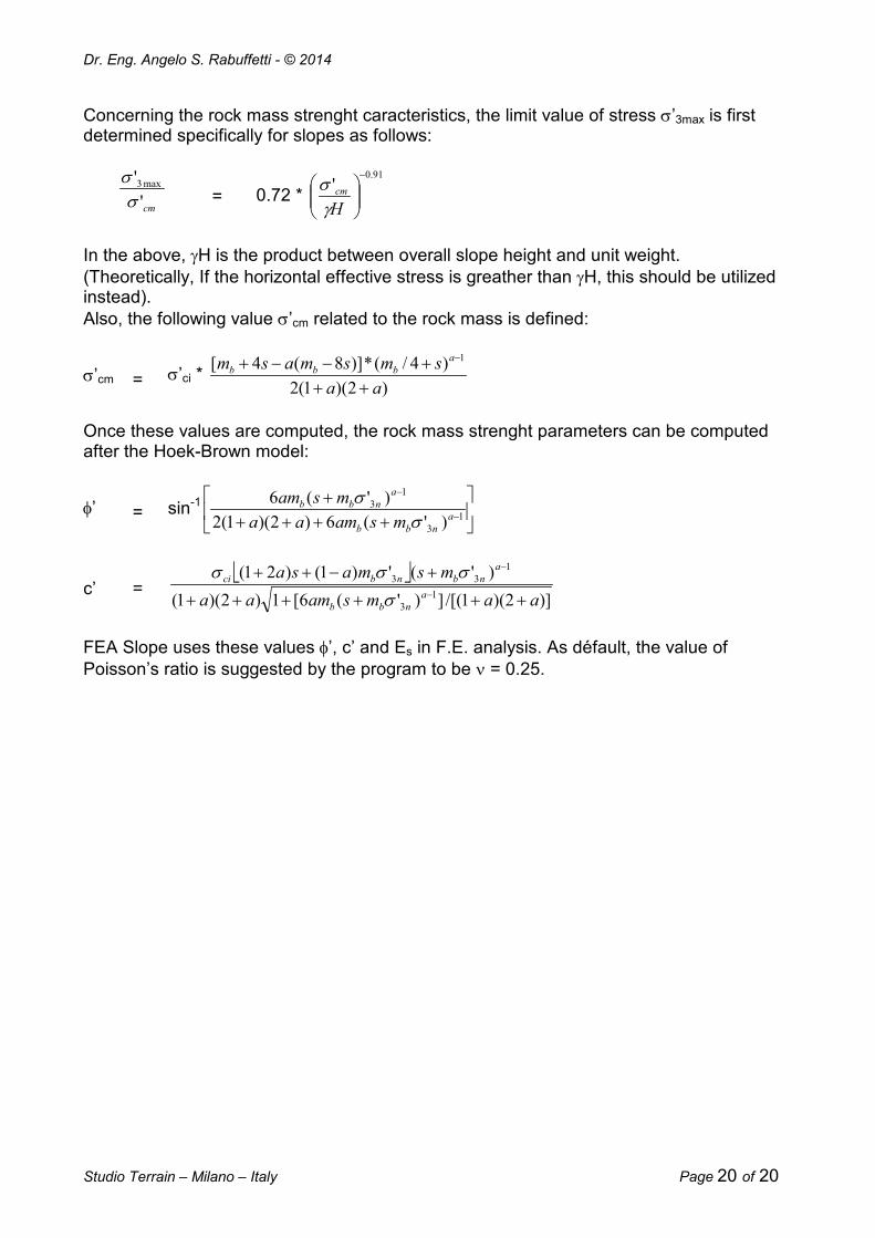
Concerning the rock mass strenght caracteristics, the limit value of stress σ’3max is first determined specifically for slopes as follows:

cm'

' max3

σσ

= 0.72 *

91.0

'−

H

cm

γσ

In the above, γH is the product between overall slope height and unit weight. (Theoretically, If the horizontal effective stress is greather than γH, this should be utilized instead). Also, the following value σ’cm related to the rock mass is defined:

σ’cm = σ’ci *

)2)(1(2

)4/(*)]8(4[ 1

aa

smsmasma

bbb

+++−−+ −

Once these values are computed, the rock mass strenght parameters can be computed after the Hoek-Brown model:

φ’ = sin-1

+++++

−

−

1

3

1

3

)'(6)2)(1(2

)'(6a

nbb

a

nbb

msamaa

msam

σσ

c’

=

)]2)(1/[(])'(6[1)2)(1(

)'(')1()21(

1

3

1

33

aamsamaa

msmasa

a

nbb

a

nbnbci

++++++

+−++−

−

σ

σσσ

FEA Slope uses these values φ’, c’ and Es in F.E. analysis. As défault, the value of Poisson’s ratio is suggested by the program to be ν = 0.25.



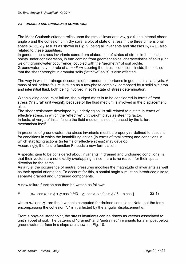
2.3 – DRAINED AND UNDRAINED CONDITIONS

The Mohr-Coulomb criterion relies upon the stress’ invariants σm, σ e θ, the internal shear angle φ and the cohesion c. In dry soils, a plot of state of stress in the three dimensional space σ1, σ2, σ3 results as shown in Fig. 9, being all invariants and stresses τxy τyz τzx also related to these quantities. In general, the stress invariants come from elaboration of states of stress in the spatial points under consideration, in turn coming from geomechanical characteristics of soils (unit weight, groundwater occurrence) coupled with the “geometry” of soil profile. Groundwater play the role of a medium steering the stress’ conditions inside the soil, so that the shear strenght in granular soils (“attritive” soils) is also affected. The way in which drainage occours is of paramount importance in geotechnical analysis. A mass of soil before failure is taken as a two-phase complex, composed by a solid skeleton and interstitial fluid, both being involved in soil’s state of stress determination. When sliding occours at failure, the budged mass is to be considered in terms of total stress (“natural” unit weight), because of the fluid medium is involved in the displacement also. The shear resistance developed by underlying soil is still related to a state in terms of effective stress, in which the “effective” unit weight plays as steering factor. In facts, at verge of initial failure the fluid medium is not influenced by the failure mechanism itself. In presence of groundwater, the stress invariants must be properly re-defined to account for conditions in which the instabilizing action (in terms of total stress) and conditions in which stabilizing actions (in terms of effective stress) may develop. Accordingly, the failure function F needs a new formulation. A specific item to be considered about invariants in drained and undrained conditions, is that their vectors are not exactly overlapping, since there is no reason for their spatial direction be the same. As a rule, the occurrence of neutral pressures modifies the magnitude of invariants as well as their spatial orientation. To account for this, a spatial angle α must be introduced also to separate drained and undrained components. A new failure function can then be written as follows: F = σm‘ cos α sin φ + σ cos θ /√3 - σ‘ cos α sin θ sin φ / 3 – c cos φ 22.1) where σm‘ and σ‘ are the invariants computed for drained conditions. Note that the term encompassing the cohesion “c” isn’t affected by the angular displacement α. From a physical standpoint, the stress invariants can be drawn as vectors associated to unit snippet of soil. The patterns of “drained” and “undrained” invariants for a snippet below groundwater surface in a slope are shown in Fig. 10.



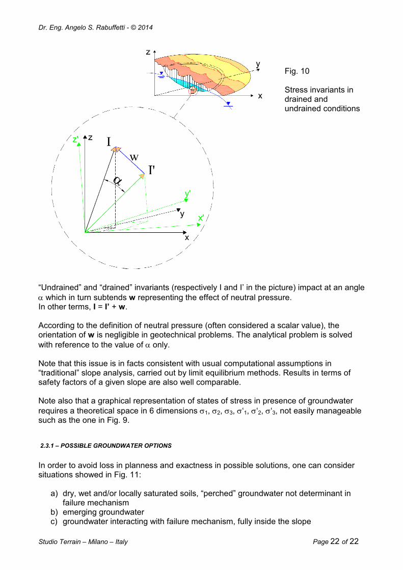
Fig. 10 Stress invariants in drained and undrained conditions

“Undrained” and “drained” invariants (respectively I and I’ in the picture) impact at an angle α which in turn subtends w representing the effect of neutral pressure. In other terms, I = I’ + w.

According to the definition of neutral pressure (often considered a scalar value), the orientation of w is negligible in geotechnical problems. The analytical problem is solved with reference to the value of α only. Note that this issue is in facts consistent with usual computational assumptions in “traditional” slope analysis, carried out by limit equilibrium methods. Results in terms of safety factors of a given slope are also well comparable. Note also that a graphical representation of states of stress in presence of groundwater requires a theoretical space in 6 dimensions σ1, σ2, σ3, σ‘1, σ‘2, σ‘3, not easily manageable such as the one in Fig. 9.

2.3.1 – POSSIBLE GROUNDWATER OPTIONS

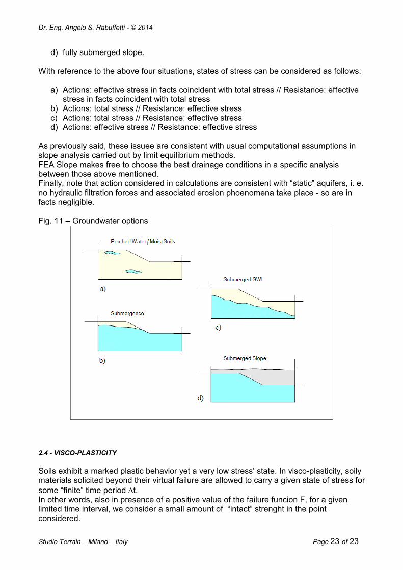
In order to avoid loss in planness and exactness in possible solutions, one can consider situations showed in Fig. 11:

a) dry, wet and/or locally saturated soils, “perched” groundwater not determinant in failure mechanism

b) emerging groundwater c) groundwater interacting with failure mechanism, fully inside the slope



d) fully submerged slope. With reference to the above four situations, states of stress can be considered as follows:

a) Actions: effective stress in facts coincident with total stress // Resistance: effective stress in facts coincident with total stress

b) Actions: total stress // Resistance: effective stress c) Actions: total stress // Resistance: effective stress d) Actions: effective stress // Resistance: effective stress

As previously said, these issuee are consistent with usual computational assumptions in slope analysis carried out by limit equilibrium methods. FEA Slope makes free to choose the best drainage conditions in a specific analysis between those above mentioned. Finally, note that action considered in calculations are consistent with “static” aquifers, i. e. no hydraulic filtration forces and associated erosion phoenomena take place - so are in facts negligible. Fig. 11 – Groundwater options

2.4 - VISCO-PLASTICITY

Soils exhibit a marked plastic behavior yet a very low stress’ state. In visco-plasticity, soily materials solicited beyond their virtual failure are allowed to carry a given state of stress for some “finite” time period ∆t. In other words, also in presence of a positive value of the failure funcion F, for a given limited time interval, we consider a small amount of “intact” strenght in the point considered.



A series of “time steps” can be considered during which the soil can resist also after the failure criterion expressed by function F is violated. Non-linear analysis can then be performed by maintaining constant the global stiffness matrix, and re-iterating numerical verifications by adapting at every step all loads acting on elements involved in failure. In other terms, for each load step, the equation’s system governing the analysis is solved by introucing loads increasingly updated: K δδδδi = Pi 24) where “i” represents the i-th iteration. Increments in displacements ui are updated after δδδδi, so that also deformations are obtained after the following deformations / displacements relationship: ∆εεεεi = B ui 25) As said, the soil flows plastically after the elastic resistance is overcome, depleting both components, elastic and plastic: ∆εεεεi = (∆εεεεe + ∆εεεεp)i 26) In this process, only elastic components ∆εεεεe can produce increase in state of stress according to the elastic relationship between stress and deformations: ∆σσσσi = De(∆εεεεe)i 27) These new stresses are added at every “time step” to the initial ones, updating the whole solving system and enabling a new run of calculations is performed for changed conditions of equilibrium / failure. At every step, a re-distribution of stresses exceeding the limit - and the failed element cannot more undergo - is carried out. New incremental “body loads” are then generated, to be added to the previous ones for a new iteration of calculations. These “body loads” are spread along the boundaries of the collapsed element (function F > 0), embroiling other elements in the incremental process. Iterations of system solving with incremental loads due to generation of “body loads” implements in facts the FEM visco-plastic analysis. Increments (and iterations) stop more or less arbitrarily when one or more convergence criterion is met by values from subsequent iteractions. As typical rule, FEA Slope considers a solution is converging when the ratio of maximum displacements coming from two consecutive solutions appears to be less than 0.0001. In the contrary, if convergence criterion isn’t meet after a reasonably high number of iterations (say 500 or 1000), calculations are stopped and the slope is considered failed. For numerical analysis pourpose, a definition of the “time step” for a unconditioned stable solution, for the Mohr-Coulomb criterion, can be taken as follows:



4 (1 + ν) (1 - 2 ν) ∆t = −−−−−−−−−−−−−−− 28) E (1 – 2ν + sin2 φ) In this way, plastic deformations eP come from a visco-plastic rate: ėVP = F ∂Q / ∂σσσσ 29) where all quantities are obtained as follows. By multiplying the visco-plastic ratio times the step ∆t, we obtain the unitary increment in plastic deformation, for the considere “step”: (δeVP)i = ∆t (δėVP)i 30) Derivative of the function of plastic potential Q with respect to the stresses σσσσ is written as: ∂Q / ∂σσσσ = ∂Q / ∂σσσσm ∂σσσσm / ∂σσσσ + ∂Q / ∂J2 ∂J2 / ∂σσσσ + ∂Q / ∂J3 ∂J3 / ∂σσσσ Besides J3 as previously defined for invariants, a new term J2 = ½ t2 is introduced. The body loads generation coming from plasticization is developed for increasing “time steps”, by summing up the following integrals for each element containing at least one collapsed Gauss point:

All

L Pi

b = Pi-1b BT De (δeVP)i dx dy 31)

∫∫ o

Elements

This process is repeated for every time interval until no more Gauss point stresses violate a convergence (failure) criterion within a fixed tolerance. This convergence criterion is based on a given amount of displacement ratio between one iteraction and the next, that can be considered allowable. FEA Slope considers is meet a convergence acceptance criterion between subsequent displacements when their ratio is less than 1/10000. Note that variation of this ratio could affect accuracy in FEM solutions. More details about visco-plasticicty in FE analysis and iterative computations can be inferred from Smith and Griffiths (1988, 2004) and Griffiths (1980).



2.5 – “ASSOCIATED” AND “NON ASSOCIATED” PLASTIC FLOW. DILATANCY

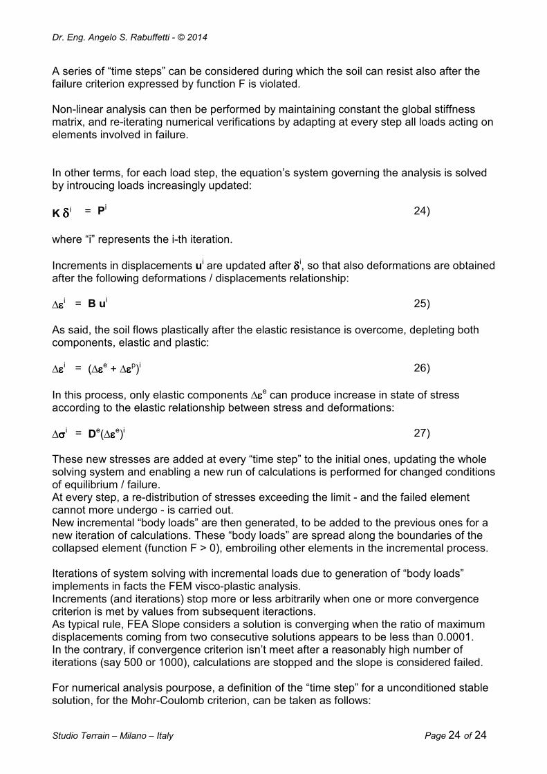
In a representation inside a p / q plane (where p = (σ1 + σ3) / 2 is the principal intermediate stress and q = (σ1 - σ3) / 2 is the deviator of stress) failure results in a rather characteristic pattern. In facts, state of stress progresses from inside to outside the perimeter of a given area. Inside the bordered area in Fig. 12, the failure function F applies. Outside the bordered area, plastic potential Q applies instead. A major issue is that the state of stress inside and outside cannot be governed by the same rules, so the plastic potential must be analytically independent from failure function. Similarly to hydraulic problems of flow across a given boundary, “flow” of stresses are considered. The “flow” is said “associated” if the vector representing plastic vector is orthogonal to both the boundaries, non plastic F and plastic Q, “non associated” in the contrary. An associated flow criterion does not warrant analytical independence. A “non associated” flow criterion is mandatory in case of presence of dense sands or overconsolidated clays. FEA Slope encompass a “non associated” plastic criterion based on use of dilatancy angle ψ in potential function Q instead the internal shear angle φ. In such a way the two functions are made reciprocally independent.

Fig. 12 - Definition of “non associated” plastic flow. Dilatancy is expressed in physical terms as the component governing the volume expansion of dense soils when a state of shear failure is reached. One can consider the peak value of internal shear angle φ made by two contributions: a shear angle φcv at constant volume and a value β depending from particle interlocking in a specimen of sand: φ = φcv + β 32) The component β, or dilatancy ψ, is a paramount factor in behaviour of granular soils at failure, notwithstanding particle shape and celerity of load application may play a certain role. In other words, dilatancy can be considered as a part of full shear resistance not depending from material’s properties. φcv can be considered constant for a specific material (calcareous sand, quartz, feldspar), so the dilatancy essentially depends upon density.



For example, the following values of peak friction angle φ, constant volume φcv, and dilatancy are summarized in Das (1985): Soil type

φ φcv β (indicative values)

Sand (rounded grains) - loose 28 – 30 2 - medium dense 30 – 35 26 – 30 4 – 5 - dense 35 – 38 8 – 9 Sand (angular grains) - loose 30 – 35 0 - medium dense 35 – 40 30 – 35 5 - dense 40 – 45 10 Gravelly sands 34 – 48 33 – 36 1 – 12 Dilatant behaviour is particularly significant in constant volume geotechnical problems (e. g. confined laboratory tests). In facts, for problems with states of stress substantially “unconfined” or scarcely confined, such as the slope stability problem, contribution of dilatancy is only relative, and the assumption y = 0 doesn’t leads significant errors. 2.6 – SEISMIC CONDITIONS

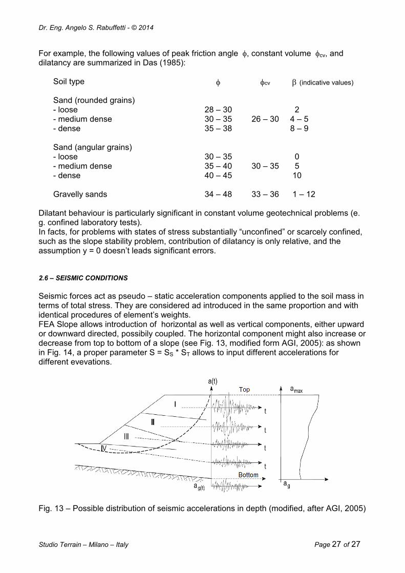
Seismic forces act as pseudo – static acceleration components applied to the soil mass in terms of total stress. They are considered ad introduced in the same proportion and with identical procedures of element’s weights. FEA Slope allows introduction of horizontal as well as vertical components, either upward or downward directed, possibily coupled. The horizontal component might also increase or decrease from top to bottom of a slope (see Fig. 13, modified form AGI, 2005): as shown in Fig. 14, a proper parameter S = SS * ST allows to input different accelerations for different evevations.

Fig. 13 – Possible distribution of seismic accelerations in depth (modified, after AGI, 2005)



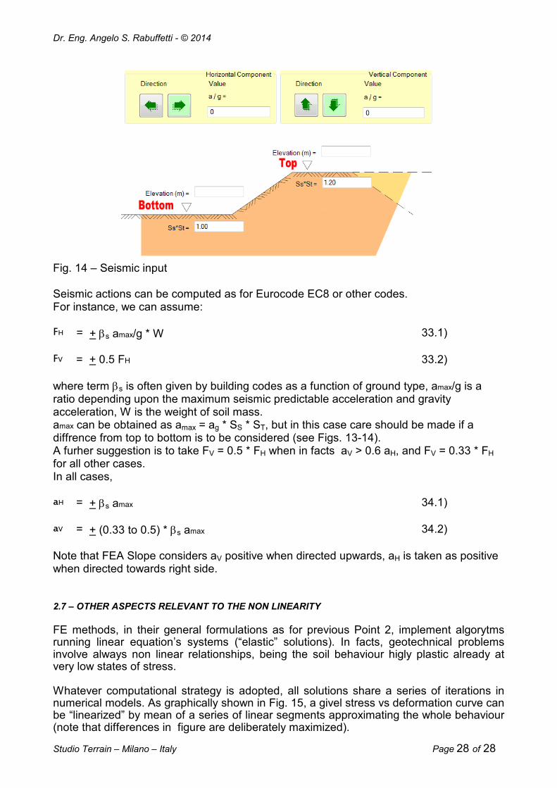
Fig. 14 – Seismic input Seismic actions can be computed as for Eurocode EC8 or other codes. For instance, we can assume: FH = + βs amax/g * W 33.1) FV = + 0.5 FH 33.2) where term βs is often given by building codes as a function of ground type, amax/g is a ratio depending upon the maximum seismic predictable acceleration and gravity acceleration, W is the weight of soil mass. amax can be obtained as amax = ag * SS * ST, but in this case care should be made if a diffrence from top to bottom is to be considered (see Figs. 13-14). A furher suggestion is to take FV = 0.5 * FH when in facts aV > 0.6 aH, and FV = 0.33 * FH for all other cases. In all cases, aH = + βs amax 34.1) aV = + (0.33 to 0.5) * βs amax 34.2) Note that FEA Slope considers aV positive when directed upwards, aH is taken as positive when directed towards right side. 2.7 – OTHER ASPECTS RELEVANT TO THE NON LINEARITY

FE methods, in their general formulations as for previous Point 2, implement algorytms running linear equation’s systems (“elastic” solutions). In facts, geotechnical problems involve always non linear relationships, being the soil behaviour higly plastic already at very low states of stress. Whatever computational strategy is adopted, all solutions share a series of iterations in numerical models. As graphically shown in Fig. 15, a givel stress vs deformation curve can be “linearized” by mean of a series of linear segments approximating the whole behaviour (note that differences in figure are deliberately maximized).



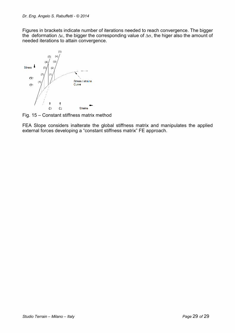
Figures in brackets indicate number of iterations needed to reach convergence. The bigger the deformation ∆ε, the bigger the corresponding value of ∆σ, the higer also the amount of needed iterations to attain convergence.

Fig. 15 – Constant stiffness matrix method FEA Slope considers inalterate the global stiffness matrix and manipulates the applied external forces developing a “constant stiffness matrix” FE approach.



3 – SLOPE STABILITY AND GEOTECHNICAL PROBLEMS 3.1 – DIFFUSION MECHANISM

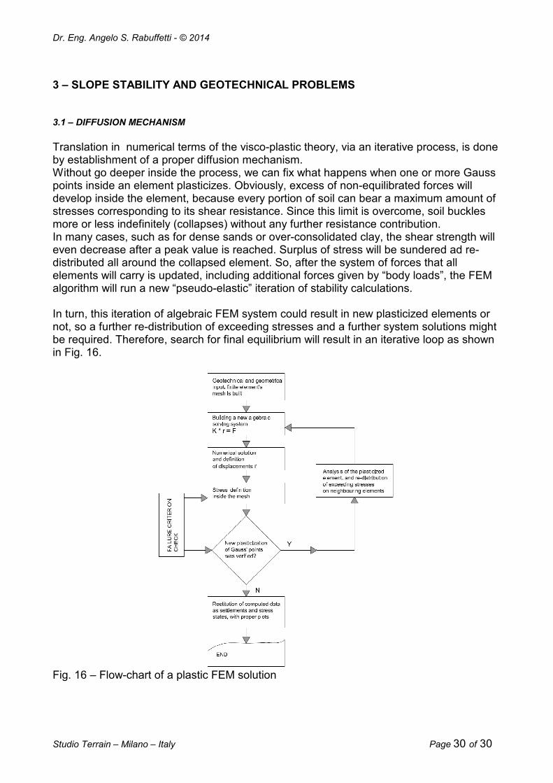
Translation in numerical terms of the visco-plastic theory, via an iterative process, is done by establishment of a proper diffusion mechanism. Without go deeper inside the process, we can fix what happens when one or more Gauss points inside an element plasticizes. Obviously, excess of non-equilibrated forces will develop inside the element, because every portion of soil can bear a maximum amount of stresses corresponding to its shear resistance. Since this limit is overcome, soil buckles more or less indefinitely (collapses) without any further resistance contribution. In many cases, such as for dense sands or over-consolidated clay, the shear strength will even decrease after a peak value is reached. Surplus of stress will be sundered ad re-distributed all around the collapsed element. So, after the system of forces that all elements will carry is updated, including additional forces given by “body loads”, the FEM algorithm will run a new “pseudo-elastic” iteration of stability calculations. In turn, this iteration of algebraic FEM system could result in new plasticized elements or not, so a further re-distribution of exceeding stresses and a further system solutions might be required. Therefore, search for final equilibrium will result in an iterative loop as shown in Fig. 16.

Fig. 16 – Flow-chart of a plastic FEM solution



Exploitation of “pseudo-elastic” solutions can be repeated also several hundreds or thousands of times before be enabled to infer if a given iterative calculus is to be considered convergent or not. From a numerical standpoint, stability will be confirmed when two different sets of results (nodal displacements), coming from two consecutive iterations, prove to be equal each other, or anyway different only by a very small amount, pre-emptively fixed. In such a situation, also despite the presence of diffuse plasticization, the slope is to be considered stable in the given conditions of soil profile, external loads, and soil resistance characteristics. In the contrary, if displacements will not converge after an arbitrary big number of solutions, iteration process will be stopped, and failure is considered to occur. 3.2 – THE GEOTECHNICAL “SAFETY FACTOR” OF THE SLOPE

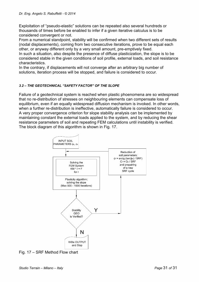
Failure of a geotechnical system is reached when plastic phoenomena are so widespread that no re-distribution of stresses on neighbouring elements can compensate loss of equilibrium, even if an equally widespread diffusion mechanism is invoked. In other words, when a further re-distribution is ineffective, automatically failure is considered to occur. A very proper convergence criterion for slope stability analysis can be implemented by maintaining constant the external loads applied to the system, and by reducing the shear resistance parameters of soil and repeating FEM calculations until instability is verified. The block diagram of this algorithm is shown in Fig. 17.

Fig. 17 – SRF Method Flow chart



The rationale of this kind of iteration is to repeat the same verification by decreasing soil resistance, until failure is reached. This method, called Strength Reduction Factor (SRF), consists of the application of a reduction factor SRF to the cohesion and to the tangent of angle of internal shear, as follows: cd = c k / SFR tan φd = atan(tan φ k)/SFR cd and tan φd, i. e. design values, are in facts utilized in calculations instead of c k and φ k (characteristic values). Once a preliminary calculation is run with SRF = 1, for which numerical convergence is supposed to be verified, value of SRF is increased (the available shear resistance is decreased) and the calculation repeated. If results will converge, the method is re-iterated by increasing from time to time the value of SRF. Algorithm will stop when soil resistance is decreased to a limit that stability is no further verified (unmatched convergence of diffusive mechanism). By rule, the computed “safety factor” will be the last value of SRF in a monotonically increasing series applied before instability is verified. Precision in determination of the safety factor will depend on how much close each other are the values inside the series.



Bibliography

- - AA. VV. (1986) "NAVFAC Design Manual 7.01 - Soil Mechanics" - US Navy,

Alexandria, Virginia - AA. VV. (1986) "NAVFAC Design Manual 7.02 - Foundations & Earth Structures" - US

Navy, Alexandria, Virginia - AA. VV. (1992) "Applicazione del calcolo automatico in Ingegneria Geotecnica" -

Politecnico di Milano - AA. VV. (1992) "Applicazione del calcolo automatico in ingegneria geotecnica" -

Politecnico di Milano - AA. VV. (1997) "NAVFAC Design Manual 7.03 - Soil dynamics and special design

aspects" - US Navy, Alexandria, Virginia - AA. VV. (2005) AGI - Associazione Geotecnica Italiana "Aspetti geotecnici della

progettazione in zona sismica - Linee guida" - AA. VV. (2006) "Canadian Foundation Engineering Manual" - The Canadian

Geotechnical Society - AA. VV. Eurocode 7 - UNI ENV 1997-1:1997 : "Geotechnical design" - Part 1 - General

rules - AA. VV. Eurocode 7 - UNI ENV 1997-2:2002 : "Geotechnical design" - Part 2 - Design

assisted by laboratory testing - AA. VV. Eurocode 7 - UNI ENV 1997-3:2002 : "Geotechnical design" - Part 3 - Design

assisted by field testing - AA. VV. Eurocode 8 - prEN 1998-5:2003 : "Design of structures for earthquake

resistance” Part 5: Foundations, retaining structures and geotechnical aspects - AGI Associazione Geotecnica Italiana (1977) "Raccomandazioni sulla programmazione

ed esecuzione delle indagini geotecniche" - AGI Associazione Geotecnica Italiana (1994) "Raccomandazioni sulle prove

geotecniche di laboratorio" - Andrus, D.R. and Stokoe, K.H., (2000) “Liquefaction Resistance of Soils from Shear-

Wave Velocity,” ASCE, Journal of Geotechnical and Geoenvironmental Engineering, Vol. 126, No. 11, November

- Bardet, J. P., Ichii, K., Lin, C. H., (2000) "EERA A computer program for equivalent-linear earthquake site response analyses of layered soil deposits" - Department of Civil Engineering, University of South California, USA

- Bishop A.W. (1955) "The use of slip circle in the stability analysis of slopes" – Geotechnique, vol. 5(1)

- Bowles J. E. (1974) "Analytical and Computer Methods in Foundation Engineering" – Mc Graw Hill Int. Ed.

- Bowles J. E. (1997) "Foundation analysis and design" - Mc Graw-Hill - Bray, J. W. (1997) "Two-dimensional boundary element stress analysis" in

Underground Excavation in Rock - E. Hoek - E.T. Brown - E & FN Spon ed. - Circ. Cons. Sup. LL. PP. 2 febbraio 2009 Nr. 617 “Istruzioni per l’applicazione delle

“Nuove norme tecniche per le costruzioni” di cui al decreto ministeriale 14 gennaio 2008”

- Cook, R. D. - Malkus D. S. - Plesha M. E. (1989) "Concepts and Applications of Finite Element Analysis" Third Edition. John Wiley & Sons,

- Das B. M. (1985) "Advanced soil mechanics" - Mc Graw Hill - Denver H. (1982) "Modulus of Elasticity for Sand Determinated by SPT and CPT" -

Proceeding of the second European Symposium on Penetration Testing, Amsterdam.



- Dupuit, J., (1863) "Etudes théoriques et pratiques sur le mouvement des eaux" - Griffiths D. V. - Fenton G. A. (2004) - "Probabilistic slope stability analysis by finite

elements" - ASCE Journal of Geotechnical and Geoenvironmental Engineering - 130(5)

- Griffiths D. V. – Lane P. A. (1999) "Slope stability analysis by finite elements" Géotechnique 49, no. 3

- Hoek E - Brown E. T. (1980) "Empirical strength criterion for rock masses" JGED ASCE - 106(GT9)

- Hoek E. - Carranza-Torres C. - Corkum B (2002) "Hoek-Brown failure criterion - 2002 Edition" Proceedings of the Fifth North American Rock Mechanics Symposium (NARMS-TAC), University of Toronto Press, Toronto

- Irons, B. M. - Zienkiewicz O. C. (1968) “The Isoparametric Finite Element System – A New Concept in Finite Element Analysis” Proc. Conf. Recent Advances in Stress Analysis. Royal Aeronautical Society. London.

- Lai C. G., Paolucci R. (2008) "L'input sismico nelle applicazioni di ingegneria geotecnica" in Opere geotecniche in condizioni sismiche a cura di G. Barla e M. Barla - Atti del XII Ciclo di Conferenze di Meccanica e Ingegneria delle Rocce (MIR 2008) - Torino

- Lai C. G., Petrini L., Strobbia C. (2006) "Prestazioni attese e descrizione dell'input sismico, logiche attuali e del prossimo futuro" - L'Edilizia No 145

- Lambe T. W., Whitman R. V. (1979) "Soil Mechanics - SI Version" - Wiley International - Lancellotta R. (1987) "Geotecnica" Zanichelli - Lancellotta R., Calavera J. (1999) "Fondazioni" Mc Graw Hill Italia, pp. 330-331 - Muskat, M., (1937) "The Flow of Homogeneous Fluids through Porous Media" - Mc

Graw-Hill Book Company - Nova R. (1981) "Basi concettuali nella pratica progettuale dei modelli costitutivi del

terreno" - RIG - Aprile - Giugno 1981 - NTC 2008 - D. M. Infrastrutture 14 gennaio 2008 “Nuove Norma Tecniche per le

costruzioni” - O.P.C.M. 20 marzo 2003 n. 3274 “Primi elementi in materia di criteri generali per la

classificazione sismica del territorio nazionale e di normative tecniche per le costruzioni in zona sismica”

- Peck R. B, Hanson W. E., Thornburn T. H. (1974) - "Foundation engineering - 2nd edition" - Wiley International

- Prandtl L. (1921) "Uber die Eindringungsfestigkeit plastisher Baustoffe und die Festigkeit von Schneiden" – Zeitschrift fur Angewandte Mathematik und Mechanik, 1, No. 1, pp15-20

- Rabuffetti A. S. (2010) "Fondazioni superficiali. Progetto e calcolo geotecnico secondo le nuove NTC" - Edizioni DEI - Roma

- Rabuffetti A. S. (2011) "Manuale di progettazione geotecnica" - Edizioni DEI - Roma - Rabuffetti A. S. (2012) "Manuale di geotecnica avanzata" - Edizioni DEI - Roma - Rabuffetti A. S. (2013) "Le analisi agli elementi finiti in geotecnica – Valutazione di

stabilità dei pendii" – Maggioli Editore – S. Arcangelo di Romagna - Rampello S., Callisto L. (2008) "Stabilità dei pendii in condizioni sismiche" in Opere

geotecniche in condizioni sismiche a cura di G. Barla e M. Barla - Atti del XII Ciclo di Conferenze di Meccanica e Ingegneria delle Rocce (MIR 2008) - Torino

- Rocchi G., Fontana M., Da Prat M. (2007) "Modelling of natural soft clay destruction process using viscoplasticiy theory" Geotechnique, vol. 53(8)

- Roscoe, K.H., and Schofield, A.N. (1963) "Mechanical behaviour of an idealized wet clay” In Proceedings of the 2nd European Conference on Soil Mechanics and



Foundation Engineering. Problems of Settlements and Compressibility of Soils, Wiesbaden, Germany. Edited by Deutsche Gesellschaft fuer Erd-und Grundbau.

- Schleicher F. (1926) "Zur Theorie des Baugrundes" – Bauingenieur, Vol. 7, pp.931-952 - Schlichting H. (1960) "Boundary Layer Theory" Mc Graw Hill Books, New York - Sichardt, W., Kyrieleis, W., (1930) "Grundwasserabsenkungen bei

Fundierungsarbeiten", Berlin - Smith I. M. - Griffiths D. V. (1988) - "Programming the finite element method" - Second

Edition - John Wiley & Sons - Smith I. M. - Griffiths D. V. (2004) - "Programming the finite element method" - 4th

Edition - John Wiley & Sons - Sowers G.B. (1970) "Introductory Soil Mechanics and Foundations" - The Macmillian

Company. - Terzaghi K. (1943) "Theoretical Soil Mechanics" John Wiley & Sons - Timoshenko S. P. (1936) "Theory of elastic stability" - Mc Graw Hill Books - Timoshenko S. P. (1936) "Theory of elastic stability" - Mc Graw Hill Books - Timoshenko S., Goodier J. N. (1951) “Theory of Elasticity” 2nd Edition, Mc Graw Hill

Books, New York - Timoshenko S., Woinowsky-Krieger S. (1959) "Theory of Plates and Shells" Mc Graw

Hill Books, New York - Wilson, E.L. (1963) “Finite Element Analysis of Two-Dimensional Structures” D. Eng.

Thesis. University of California at Berkeley. - Winterkorn H. F., Fang H-Y (1975) "Foundation Engineering Handbook" - Van

Nostrand Reinhold New York - Zienkiewicz O. C. – Taylor R. L. (1989) "The Finite Element Method, Vol. 1, basic

formulation and linear problems" Mc Graw Hill Book Europe, Maidenhead, GB - Zienkiewicz O. C. – Taylor R. L. (1991) "The Finite Element Method, Vol. 2, solid and

fluid mechanics, dynamics and non-linearity" Mc Graw Hill Book Europe, Maidenhead, GB