1
1
Fourier transform of continuous-timesignals
Spectral representation of non-periodic signals
2
Fourier transform: aperiodic signals
• repetition of a finite-duration signal x(t)=> periodic signals.
• Periodic signal (T → ∞) => non-periodic signal x(t)
( ) ( ) ( ) ( ) ( ) ( )Tk k
x t x t t x t t kT x t kT∞ ∞
=−∞ =−∞= ∗δ = ∗ δ − = −∑ ∑
( ) ( )T
x t x t→∞→

2
3
Non-periodic signal & periodic signal, period T.
Non-periodic
Periodic
repetition T → ∞
( ) ( )111
0 otherwiseT, t T
x t p t,
Δ ⎧ ≤= = ⎨
⎩
4
( ) ( )T
x t x t→∞→
3
5
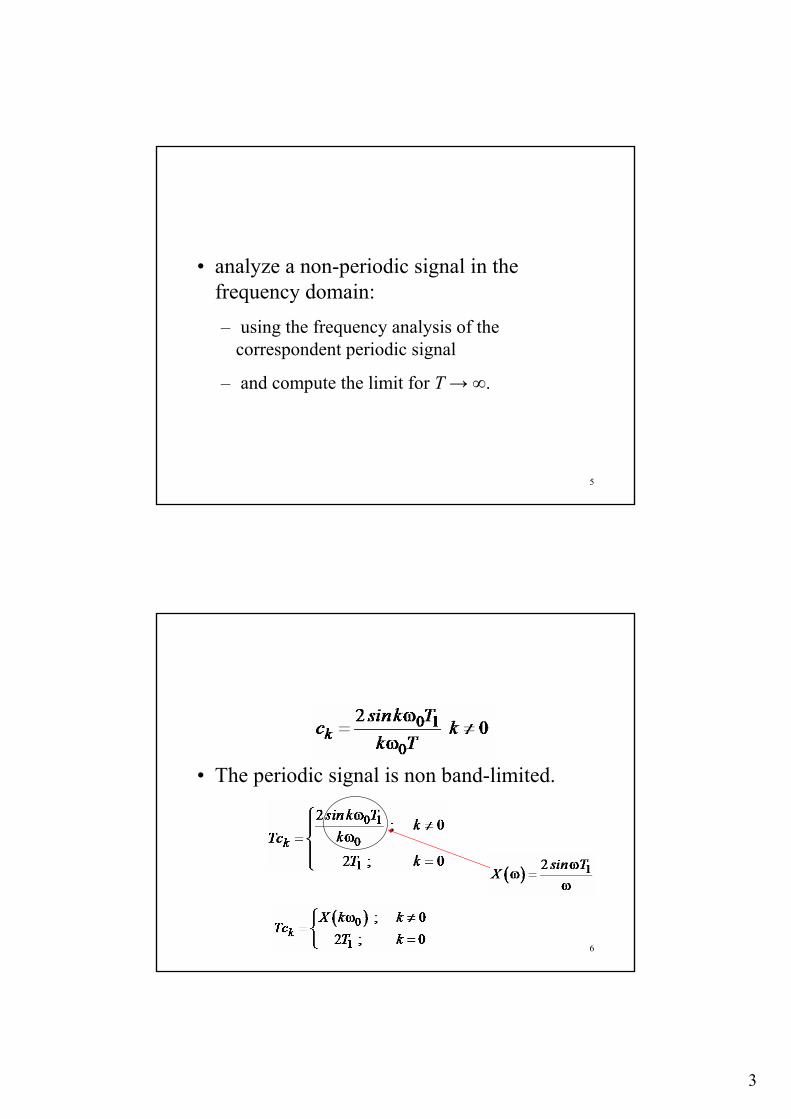
• analyze a non-periodic signal in the frequency domain:– using the frequency analysis of the
correspondent periodic signal
– and compute the limit for T →∞.
6
• The periodic signal is non band-limited.

4
7
The product T⋅ck & the envelope
X(ω) = envelope for T⋅ck
Relation between them?
8
General case
• the Fourier coefficients of the periodic signal :
( ) 02
2
1 Tjk t
kT
c x t e dtT
− ω
−= ∫
( ) 02
2
1 Tjk t
kT
c x t e dtT
− ω
−= ∫
Equal on [-T/2, T/2]

5
9
Fourier transform• outside [-T/2,T/2] the non-periodic signal =0
• With the function:( ) 01 jk t
kc x t e dtT
∞− ω
−∞= ∫
( ) ( ) j tX x t e dt∞
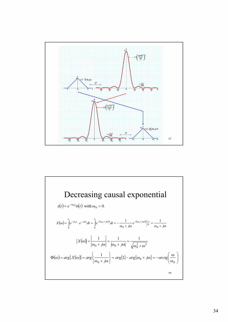
− ω
−∞ω = ∫
( )0 01 2 kc X k ,T T
π= ω ω =
(The envelope of T⋅ck )
10
Square wave:different values of T

6
11
Remarks
• The envelope is not affected by T. • Increase T ⇒ spectral components are “closer”. • T→∞ ⇒
– distance→0– the discrete spectral representation becomes
continuous. – the periodic signal → non-periodic.
12
Definition
• Fourier pair
( ) ( ) ( ) ( )1 2
j t j tx t X e d X x t e dt∞ ∞
ω − ω
−∞ −∞= ω ω ↔ ω =
π ∫ ∫
Fourier Transform(spectrum)
Inverse Fourier Transform

7
13
Remarks
• periodic signals : spectral lines
• non-periodic signals spectra are continuous
( )0 01 2 kc X k ,T T
π= ω ω =
14
CTFT for signals in the class L1
• for signals in L1, the Fourier transform is not necessarily from L1
• Reconstruction theorem!

8
15
• the Fourier transform is convergent (the signal x(t)∈L1) but X(ω)∉L1.
• the reconstruction of the signal from its spectrum is not obvious.
( )ωωsin2ω τ
=X( ) ( ) ( ) ( )ττ −−== tttptx σσ
( ) ∞<=∫∞
∞−2dttpτ
16
Reconstruction theorem
• If the signal x(t) belongs to L1 and has bounded variation on the entire real axis then its Fourier transform can be inverted using :
( ) ( ){ }( ) ωω ω detxtx tjR
RR⋅= ∫
−∞→
1lim F

9
17
1. Linearity
• If x(t) and y(t) ∈ L1 and have the Fourier transform X(ω) and Y(ω) then for any complex constants a and b the signal ax(t)+by(t) ∈ L1 and has the Fourier transform aX(ω)+bY(ω).
Homework: Prove it.
( ) ( ) ( ) ( )ωω bYaXtbytax +→+
18
2. Time Shifting
• Time shifting -> modulation in frequency (multiplication with a complex exponential).
• Proof
( ) ( )00
j tx t t e Xω ω−− ↔
( ){ } ( ) ( ) ( ) ( ). F ωττ ωτωτ
ω Xedexdtettxttx tjtjtt
tj 000
001 −+−
∞
∞−
−=∞
∞−
− =⋅=⋅−=− ∫∫

10
19
Remarks
• Fourier transform: complex function.
• The Fourier transform H(ω) of the impulse response h(t) of a system: frequency response.
• frequency dependence of the magnitude of H(ω) = magnitude characteristic of the system |H(ω)|
• frequency dependence of the argument of H(ω) = phase characteristic of the system arg{H(ω)}
20
3. Modulation
• Modulation in time -> shifting in frequency.
• Proof
( ) ( )00 .j te x t Xω ω ω→ −
( ){ } ( )
( ) ( ) ( )
( ) ( ).0
0
1
0
0
00
ωω
ωω
ω
ωω
ωωω
−→
−=⋅=
=⋅⋅=⋅
∫
∫
∞
∞−
−−
−∞
∞−
Xtxe
Xdtetx
dteetxetx
tj
tj
tjtjtjF

11
21
Duality
• operation in time ⇒ another operation in frequency : – modulation ⇒ shifting (3rd property)
• 2nd operation in time ⇒ first operation in frequency. – time shifting ⇒ modulation (2nd property)
• This behavior is named duality.
22
4. Time Scaling
• If x(t) ∈ L1 ⇒ its scaled version x(t/a) ∈ L1
and the spectrum of x(t/a) is a frequency scaled version of the spectrum of x(t).
• the scaling is an auto-dual operation.
( ) 1 .x at Xa a
ω⎛ ⎞→ ⎜ ⎟⎝ ⎠

12
23
• Proof
( ){ } ( ) ( )
( ) .1
;111
⎟⎠⎞
⎜⎝⎛→
⎟⎠⎞
⎜⎝⎛=⋅=⋅=
−∞
∞−
∞
∞−
=− ∫∫
aX
aatx
aX
adex
adteatxatx a
jattj
ω
ωτττωτωF
24
Example: the square wave
• spectrum
• its time-scaled variant , a=2:
• a=1/2( )2
1 2 2 2212 22
sin sinp t p tτ τωτ ωτ⎛ ⎞ = ↔ =⎜ ⎟ ω ω⎝ ⎠
( ) 2 sinp tτωτ
↔ω
( ) ( )2
22 2 22 =2
2
sin sinp t p tτ τ
ω ωτ τ= ↔
ω ω

13
25
time compression → frequency dilation
time dilation → frequency compression
26
CTFT of the constant distribution
( ) ( )F
1 2t πδ ω↔

14
27
Proof
• the constant distribution can be approximated:
• We know that
( ) ( )ttp 1lim =∞→
ττ
( )ωωτω
τsin2=⋅∫
∞
∞−
− dtetp tj
( )ωωτ
τω
ττ
sin2limlim∞→
−∞
∞−∞→=⋅∫ dtetp tj
( )⎩⎨⎧
≠=∞
==⋅∞→
−∞
∞−∫ 0,0
0,sin2lim1ωω
ωτωττ
τω dtet tj
28
• The area under the graphical representationof the spectrum:
• So:
• and:
( ) πωωτ
ωττ 24sinsin2sin20
0=∞=⎟
⎟⎠
⎞⎜⎜⎝
⎛+== ∫∫∫
∞
∞−
∞
∞−Sidu
uudu
uudA
( )⎩⎨⎧
≠=∞
=⋅ −∞
∞−∫ 0,0
0,1
ωωω dtet tj
π2=A
( ) ( ) ( ) ( )ωπδωπδω 2121F↔⇔=⋅ −
∞
∞−∫ tdtet tj

15
29
• An immediate consequence: a new representative string for the Dirac distribution:
( )sinlimτ→∞
ωτ= δ ω
πω
30
5. Complex Conjugation
• complex conjugation in time -> reversal and complex conjugation in frequency.
• Proof
( ) ( )* *x t X ω↔ −1F
( ){ } ( ) ( ) ( ) ( )
( ) ( )ω
ωωω
−↔
−=⎥⎥⎦
⎤
⎢⎢⎣
⎡⋅=⋅= ∫∫
∞
∞−
−−−∞
∞−
**
**
*1
1
*
Xtx
Xdtetxdtetxtx tjtj
F
F

16
31
6. Time Reversal
• Time reversal -> reversal in frequency.
• Homework. Prove it.
( ) ( )ω−↔− Xtx1F
32
7. Signal’s Derivation
• Time differentiation -> multiplication with jωin frequency.
( ) ( )ωω Xjtx ⋅↔1
'F

17
33
Proof:
Integrating by parts:
the signal is in L1 :
So:
( ){ } ( ) dtetxtx tjω−∞
∞−⋅= ∫ ''1F
( ){ } ( ) ( ) dtetxjetxtx tjtj ωω ω −∞
∞−
∞
∞−− ⋅+⋅= ∫'1F
( ) ( ) 0limlim ==⋅±∞→
−
±∞→txetx
ttj
tω
( ) ( )ωω Xjtx ⋅↔1
'F
34
8. Signal’s Integration
• For x(t) ∈ L1 with X(0)=0 (no DC component), its integral ∈ L1
• Time integration -> multiplication with
1/ jω in frequency
( ) ( ) ( )1F
for 0 0t X
x d Xjω
τ τω−∞
↔ =∫

18
35
Proof
• We have: • Apply for y(t) the differentiation property:
• Y defined in 0 :
• So:
( ) ( ) ττ dxtyt∫∞−
=
( ) ( ) ( ) ( ) ( ) ( )ωωωωωω
jXYXYjtxty =⇒=↔=
1
'F
( ) 00 =X
( ) ( )ωωττ
jXdx
t 1F↔∫
∞−
36
9. Signals’ convolutionconvolution theorem
• the convolution of two signals from L1
belongs to L1.
• convolution of two signals in time -> product in frequency.
( ) ( ) ( ) ( )x t y t X Yω ω∗ ↔ ⋅1F

19
37
( ) ( ){ } ( )( ) ( ) ( )
( ) ( ) ( ) ( ) ( )
( ) ( ) ( ) ( )ωω
τττττ
τττ
ωωτττωωτ
ωω
YXtytx
dueuydexdtdetxex
dtedtyxdtetyxtytx
ujjuttjj
tjtj
⋅↔∗
⋅⋅=⋅−⋅⋅=
=⋅⎥⎥⎦
⎤
⎢⎢⎣
⎡−=⋅∗=∗
∫∫∫ ∫
∫ ∫∫
∞
∞−
−−∞
∞−
=−−−−
∞
∞−
∞
∞−
−∞
∞−
∞
∞−
−∞
∞−
1
.
1
F
F
Proof:
38
convolution of two rectangular pulses, same duration= a triangle
( ) ( ) ( )2 2
1t
p t p t p tτ τ τ⎛ ⎞
∗ = τ −⎜ ⎟τ⎝ ⎠
Example. Triangle’s spectrum
( )2
2 22
2
sin sinp tτ
ωτ ωτ
↔ = τωτω
( )
2
2 21
2
sintp tτ
ωτ⎛ ⎞⎜ ⎟⎛ ⎞
τ − ↔ τ⎜ ⎟ ⎜ ⎟ωττ⎝ ⎠ ⎜ ⎟⎝ ⎠
(convolution theorem)
20
39
40
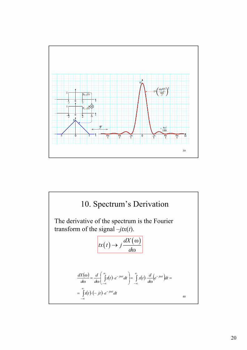
10. Spectrum’s Derivation
The derivative of the spectrum is the Fourier transform of the signal –jtx(t).
( ) ( )ωω
dXtx t j
d→
( ) ( ) ( ) ( )
( ) ( )∫
∫∫∞
∞−
ω−
ω−∞
∞−
∞
∞−
ω−
⋅−⋅=
=ω
⋅=⎟⎟⎠
⎞⎜⎜⎝
⎛⋅
ω=
ωω
dtejttx
dteddtxdtetx
dd
ddX
tj
tjtj

21
41
•The spectrum of a real and even signal is real and even.•The spectrum of a real and odd signal is imaginary and odd.
11. CTFT of Real Signals. Properties.(The Spectrum of the Even and Odd Parts of a Real Signal)
( ) { }{ } ( )( ) ( ){ } ( )
Re = and
Ime E
o O
x t X X
x t j X jX
ω ω
ω ω
↔
↔ =
42
Proof
• the real signal x(t) with spectrum X(ω), complex :
• Its complex conjugate real
( ) ( ) ( ) ( ){ } ( ){ }Re ImjX X e X j Xωω ω ω ωΦ= ⋅ = +
Polar form Cartesian form
( ) ( )ω−↔ ** Xtx
( ) ( ) ( ) ( ){ } ( ){ }* Re ImjX X e X j Xωω ω ω ω− Φ −− = − ⋅ = − − −
Polar form Cartesian form

22
43
•For real signals:
•By identification:
( ) ( ) ( ) ( )* *x t x t X Xω ω= ⇒ − =
( ) ( ) ( ) ( )( ){ } ( ){ } ( ){ } ( ){ }
; ;
Re Re ; Im Im .
X X
X X X X
ω ω ω ω
ω ω ω ω
= − Φ = −Φ −
= − = − −
Magnitude and real part of spectrum are even functions
Phase and imaginary part of spectrum are odd functions
44
Example - odd real signal ( ) 2 2
2 2
222 2
j jsinx t p t p t e e
ωτ ωτ−
τ τ
ωτ ⎛ ⎞τ τ⎛ ⎞ ⎛ ⎞ ⎜ ⎟= − − + ↔ −⎜ ⎟ ⎜ ⎟ ⎜ ⎟ω⎝ ⎠ ⎝ ⎠⎝ ⎠
The spectrum of a real and odd signal is imaginary and odd

23
45
time shifting
( )ω
ωτ
↔τ22
2
sintp
( ) 2 2sin 1 cos22 2
j jx t e e j
ωτ ωτ−
ωτ⎛ ⎞ − ωτ
↔ − = −⎜ ⎟ω ω⎝ ⎠
ω
ωτ
↔⎟⎠⎞
⎜⎝⎛ τ
+ω
ωτ
↔⎟⎠⎞
⎜⎝⎛ τ
−ωτ
τ
ωτ−
τ22
2 and 22
22
2
2
2
sinetp
sinetp
jj
Euler’s relationsin2(u) =1-cos (2u)
46
12. A Parseval like theorem for signals from L1
equivalent form:
( ) ( ) ( ) ( ) ωωω=∫ ∫∞
∞−
∞
∞−
dYxdttytX
( ){ }( ) ( ) ( ) ( ){ }( )x t y t dt x y t dω ω ω ω∞ ∞
−∞ −∞
=∫ ∫1 1F F
Fourier transform of thesignal x(t) with thevariable t
Signal x(t) withvariable ω

24
47
(see previous slides)
13. Relation Fourier Transform of a non-periodic signal & exponential Fourier series coefficients of the
periodic signal
( )0 01 2 kc X k ,T T
π= ω ω =
48
Example
( ) ⎟⎠
⎞⎜⎝
⎛ +−⎟⎠
⎞⎜⎝
⎛ −=220
2
0
200
Ttp
Ttptx TT

25
49
the spectrum of the signal x(t):
Applying the property 13:
0 0
0 0
1 cos2 1 cos2 2xk
k Tj kc j
T k k
ω− − π
= − ⋅ = − ⋅ω π
( )01
22
TcosX j
ω−
ω = −ω
50
The Fourier transform of a signal from L1 ∩ L2 is from L2
the energy of a signal in the frequency / time domain. (Parseval or Rayleigh relation)
|X(ω)|2 = energy density.
using the L2 norm:
( ) ( )2 22X d x t dtω ω π
∞ ∞
−∞ −∞
=∫ ∫
( ) ( ) 22
22 2 txX π=ω
1) finite energy signals x(t) ∈ L1 ∩ L2

26
51
Proof
If x(t) ∈ L1 ∩ L2 ⇒ x*(-t) ∈ L1 ∩ L2.Their convolution belongs to L1.
So, it has Fourier transform, Y(ω). from the convolution theorem :
( ) ( ) ( )txtxty * −∗=
( ) ( ) ( )( ) ( ) ( ) ( ) 2ω=ω⋅ω=ω−−⋅ω=ω XXXXXY **
52
We have:
for t=0:
So:
In consequence the function X(ω) belongs to L2.
( ) ( ) ( ) ( ) τ−ττ=ω⋅ωπ
= ∫∫∞
∞−
∞
∞−
ω dtxxdeYty *tj
21
( ) ( ) ( ) ( ) τττ=ωωπ
= ∫∫∞
∞−
∞
∞−
dxxdXy *2
210
( ) ( )22 0 finiteX d yω ω π
∞
−∞
= −∫

27
53
•the Fourier transform of a finite energy signal:
•The L2 norm of the Fourier transform :
( ){ }( ) ( )2 l.i .m. j tx t x t e dtτ
− ω
τ→∞−τ
ℑ ω = ⋅∫
( ){ }( ) ( )2
22 ∫
τ
τ−
ω−
∞→τ⋅=ωℑ dtetxlimtx tj
Fourier transform in L2 space convergence in mean square
2) finite energy signals x(t) ∈ L2 \ L1
54
•Truncation x(t) by multiplication with pτ(t)
⇒approximation of x(t) ∈ L1 ∩ L2
Two approximations. •The “better” one -longer support. •The other -an approximation of the first. •The error tends to zero if the two durations tend to infinity.

28
55
the approximation error
Parseval
limit for
( ) ( ) ( ) ( )( ) 2121
LLtptptxty ∩∈−= ττ
( ) ( ){ }( ) ( ) ( ){ }( )
( ) ( ) ( ) ( ) ( ) ( )∫∫τ
τ
τ−
τ−ττ
ττ
π+π=−π=
=ωℑ−ωℑ
1
2
2
1
21
21
222
2
2
211
222 dttxdttxtptxtptx
tptxtptx
2121 τ>τ∞→τ ,,
( ) ( ) 0
2
2
1
1
2
221
21
=⋅−⋅∫ ∫τ
τ−
τ
τ−
ω−ω−
τ>τ∞→τ
dtetxdtetxlim tjtj
,
( ) ( ) ( ){ }1j tx t e dt x t p tτ
ωτ
τ
−
−
⋅ → ℑ∫ in mean square.
56
Plâncherel’s Theorem
The Fourier transform definition of a finite energy signal already given can be found under the name of Plâncherel’s Theorem:

29
57
i) Plâncherel’s theorem shows that the Fourier transform of any finite energy signal belongs to L2.
ii) The Fourier transform on L2 is a particular case of the Fourier transform on L1. All the properties of the Fourier transform on L1
are verified by the Fourier transform on L2.
The Parseval’s relation - proved for signals in L1 ∩ L2 .
It is not verified by signals in L2 – L1
iii) The Parseval’s relation can be generalized on L2, in the form:
( ) ( ) ( ) ( )ωωπ
= Y,Xty,tx21
Plâncherel’s Theorem
58
the definition of the scalar product on L2:
If the two signals are equal :
Parseval’s relation.
( ) ( ) ( ) ( ) ωωωπ
= ∫∫∞
∞−
∞
∞−
dYXdttytx **
21
( ) ( )2 212
x t dt X dω ωπ
∞ ∞
−∞ −∞
=∫ ∫

30
59
14. Spectrum’s Convolution
• The convolution of the Fourier transforms X(ω) and Y(ω) gives the Fourier transform of the product x(t) y(t) multiplied by 2π.
• The convolution of two finite energy signals is of finite energy. Convolvingtwo finite energy spectra X(ω) and Y(ω) ⇒ a finite energy spectrum Z(ω)
( ) ( ) ( ) ( ){ }( )2X Y x t y tω ω π ω∗ = F
60
( ) ( ) ( ) ( ) ( )
( ) ( ) ( )122
j u t
Z X Y X u Y u du
X u y t e dt duω
ω ω ω ω
ππ
∞
−∞
∞ ∞− −
−∞ −∞
= ∗ = −
⎡ ⎤= ⋅⎢ ⎥
⎣ ⎦
∫
∫ ∫
( ) ( ) ( ) dtedueuXtyZ tjuj ω−∞
∞−
ω∞
∞−
⋅⎥⎥⎦
⎤
⎢⎢⎣
⎡⋅
ππ=ω ∫∫ 2
12
( ) ( ) ( )∫∞
∞−
ω−⋅π=ω dtetytxZ tj2
Inverse Fourier transform of X = x(t)
the Fourier transform of the product x(t)·y(t).

31
61
15. Duality
The inverse Fourier transform :For t = –t :
Applying two times the Fourier transform ⇒a reversed variant of the original signal weighted by 2π.
( ) ( ) ω⋅ω=π ω∞
∞−∫ deXtx tj2
( ) ( )2 , dualityj tx t X e d∞
− ω
−∞
π − = ω ⋅ ω∫
( ) ( ){ }( ){ }( )ttxtx ωℑℑ=−π 222
Fourier transform of X(ω).
62
double change of variables:
Using the two forms of duality we can compute the spectrum of a signal.
( ) ( ) ω⋅ω=−π ω−∞
∞−∫ deXtx tj2
tt →ωω→ and
( ) ( ) ( ){ }( )2 , another form of
duality.
j tx X t e dt X t∞
− ω
−∞
π −ω = ⋅ = ℑ ω∫
15. Duality

32
63
•Start from a known pair (x(t), X(ω))
•What is the spectrum of the signal X(t)?
•Change the variable and constants of time with variable and constants of frequency and vice versa
•obtain the corresponding pair (X(t), 2πx(-ω)).
64
The Fourier Transform of signalsTemporal window
the spectrum
In this case,
Changing the variables and constants
( ) ( ) ( ) . 2τ ωωτ
↔τ−σ−τ+σ=sintttp
( ) ( ) ( ) . 2 and τ ωωτ
=ω=sinXtptx
ω↔t 0ω↔τ
( ) 0sin2 tX ttω
= ( ) ( ) . 220
ωπ=ω−π ωpx

33
65
66
Symmetric triangular signalthe spectrum
( ) ( ) .
2
21
2
⎟⎟⎟⎟
⎠
⎞
⎜⎜⎜⎜
⎝
⎛
ω
ω
↔⎟⎟⎠
⎞⎜⎜⎝
⎛−=
Tsintp
Tt
Tttri TT
( ) ( ) ( ) .
2
2 and
2
⎟⎟⎟⎟
⎠
⎞
⎜⎜⎜⎜
⎝
⎛
ω
ω
=ω=
TsinXttritx T
( )
2
2
20
⎟⎟⎟⎟
⎠
⎞
⎜⎜⎜⎜
⎝
⎛ ω
=t
tsintX ( ) ( ). 22
0ω⋅π=ω−π ωtrix
34
67
68
Decreasing causal exponential( ) ( ) .tetx t 0 with 0
ω0 >ωσ= −
( ) ( ) ( )ω+ω
=ω+ω
−==⋅=ω ∞ω+ω−∞
ω+ω−∞
ω−ω− ∫∫ je
jdtedteeX tjtjtjt
00
000
11000
( )22
000
111
ω+ω=
ω+ω=
ω+ω=ω
jjX
( ) ( ){ } { } { } ⎟⎟⎠
⎞⎜⎜⎝
⎛ωω
−=ω+ω−=⎭⎬⎫
⎩⎨⎧
ω+ω=ω=ωΦ
00
011 arctgjargarg
jargXarg

35
69
( )22
0
1
ω+ω=ωX
( ) ⎟⎟⎠
⎞⎜⎜⎝
⎛ωω
−=ωΦ0
arctg
70
Decreasing non-causal exponential( ) ( ) .tetx t 0 with 0
ω0 >ωσ= −
( ) ( ) .tetx t 0 with 0ω0 >ω−σ=
( ) ( ) .j
XXω−ω
=ω−=ω0
1
( ) ( )22
0
1
ω+ω=ω=ω XX ( ){ } .arctg
jargXarg ⎟⎟
⎠
⎞⎜⎜⎝
⎛ωω
=⎭⎬⎫
⎩⎨⎧
ω−ω=ω
00
1

36
71
Symmetric decreasing exponential
( ) 10 ; 00 0
ω0
00 <ω<
⎪⎩
⎪⎨⎧
≤≥
== ω
ω−−
t,et,eetx t
tt
s
( ) ( ) ( ).txtxtxs +=
( ) ( ) ( ) 220
0
00
211ω+ω
ω=
ω−ω+
ω+ω=ω+ω=ω
jjXXX s
72

37
73
Gaussian signal
0. , 2
241
>π
↔ω−− ae
ae aat
The spectrum of a Gaussian signal is Gaussian
74
The Fourier Transform of Distributions
1) The spectrum of the Dirac’s distributionfor any test function ϕ(t):
the Dirac’s distribution is even.
Hence, we have obtained:
( ) ( ) ( ) ( ) ( ) ( )0or 0 ϕ=−δϕϕ=δϕ ∫∫∞
∞−
∞
∞−
dtttdttt
( ) ( ) ( ){ }( ) 1j t j tt e t e dt tω∞
− − ω
−∞
ϕ = ⇒ δ ⋅ = ℑ δ ω =∫
( ) ( )ω↔δ 1t

38
75
2) The spectrum of the constant 1(t) duality⇒ ( ) ( ) ( )ωπδ=ω−πδ↔ 221 t
( )ωδπ↔ cc 2
76
3) The spectrum of the unit step σ(t)( ) ( )1 1sgn and .
2 2u t t v t= =
( ){ }( ) ( ){ }( ) . 1=ωδℑ=ωℑ tt'u
( ){ }( ) ( ){ }( ) ( ) ( ) ( )' 1u t
u t t u t v tj j
ωω σ
ω ωℑ
ℑ = = ⇒ = +
( ){ }( ) ( )1tj
ℑ σ ω = + πδ ωω

39
77
4) The spectrum of sgn(t)
{ } ( ){ }ω
=ℑ=ℑj
tutsgn 22
1, 0sgn 0, 0
1, 0
tt t
t
>⎧⎪= =⎨⎪− <⎩
78
5) The spectrum of the signal 1/(πt)
(duality)
ω↔
jtsgn 2
( ) ωπ−=ω−π↔ sgnsgnjt
222
, 01 sgn 0, 0
, 0
jj
tj
− ω >⎧⎪↔ − ω = ω =⎨π ⎪ ω <⎩

40
79
80
6) Fourier Transform of the integral of a signal having DC component, X(0)≠0
• Proof:
( ) ( ) ( ) ( ) ττστττ dt-xdxtyt
∫∫∞
∞−∞−==
( ) ( ) ( ){ }( ) ( ) ( ) ( ) ( ) ( )ω1ω ω ω ω πδ ω π ω δ ωω ω
XY X t X X
j j⎡ ⎤
= ⋅ℑ σ = + = +⎢ ⎥⎣ ⎦
( ) ( ) ( ) ( )ωδ0πωωττ X
jXdx
t+↔∫
∞−
( ) ( ) ( ) ( )ωδ0ωδω ⋅=⋅ XX

41
81
7) The spectrum of the complexexponential
( ) ( )ωπδ21 ↔t
( )0ω ω-ωπδ20 ↔tje
Modulation:
82
8) The spectrum of cosω0t( ) ( )
0 0ω ω
0 0 0cosω π δ ω-ω δ ω ω2
j t j te et−+
= ↔ + +⎡ ⎤⎣ ⎦

42
83
( ) ( )
( ) { } ( ){ }
( ) ( )
( ) ( )( )
( )( )
0
0
0 0
0 0
0 0
12
1 22
x t cos t p t
X cos t p t
sin
sin sinX
τ
τ
= ω ⋅
ω = ℑ ω ∗ℑπ
ωτ⎡ ⎤= δ ω − ω + δ ω + ω ∗⎣ ⎦π ω
⎡ ⎤ω − ω τ ω + ω τω = τ +⎢ ⎥
ω − ω τ ω + ω τ⎢ ⎥⎣ ⎦
Spectrum for a limited cosine of duration 2 τ
84

43
85
9) The spectrum of sinω0t( ) ( )0 0ω ω
0 00
2πδ ω-ω 2πδ ω ωsinω
2 2
j t j te etj j
− − +−= ↔
( ) ( )0 0 0sin π δ ω-ω δ ω ωt j↔ − − +⎡ ⎤⎣ ⎦ω
86
Fourier transform of periodic signals• The periodic signal y(t) =convolution of its restriction at one period,
x(t) and the periodic Dirac’s distribution
• the Fourier transform of periodic δ T0(t) with period T0
-proportional with the periodic δ ω0(t) with period ω0.
( ) ( )0ω0 0 ω0
0
1δ ω δ ωjk tT
kt e
T
∞−
=−∞
= ↔∑( ) ( ) ( )ttxty T0δ∗=

44
87
( ) ( )0ω0 0
0
1δ δjk tT
k kt e t kT
T
∞ ∞−
=−∞ =−∞
= = −∑ ∑
But:
So:
( ){ }( ) ( ){ }( )∑∞
−∞=ℑ=ℑ
kT t-kTt ωδωδ 00
( ) ( ) 0ω0δ and 1δ tjet-tt −↔↔
( ){ }( ) ∑∞
−∞=
−=ℑk
TjkT et 0
0ωωδ
( ){ }( )0
δ ωT tℑ
( ) ∑∞
−∞=
−=k
tjkT e
Tt 0ω
00
1δ
00 ω and ω ↔↔ Tt
( ) ∑∞
−∞=
−=k
Tjke 0ω
00ω ω
1ωδVariable and
constant changes
88
( ) ( ) ( ){ }( ) ( ) ( )ωδωωωδωω 0ω00 ⋅⋅=ℑ⋅= XtXY T
We have the relation Fourier coefficients of the periodic signal y(t) with the Fourier transform of the non-periodic signal x(t):
The Fourier transform of the periodic signal is:
( ) ( ) ( )000
ω-ωδωπ2ω kkXT
Yk
∑∞
−∞=⋅=
( )0
0ωTkX
c yk =
( ) ( )0ω-ωδπ2ω kcY yk
k⋅⋅= ∑
∞
−∞=

45
89
The effect of signal’s truncation
( ) ( )
( ) ( ) ( )
( ) ( ) ( )( )
( )
( ) ( )
( ) ( ) ( )( ) ( ){ } ( ){ }
0
0
00
0
00
0
0
0
0 0
sin
sin 1 sin ˆ22
1 sin 1 sin 1ˆ Si
1 1Si Si
ˆ converges in mean square to :
. . .
tx t pt
t p t p Xt
u uX p u du du yu u
X X p
l i m x t p t x t
++∞
−−∞ −
→∞
= ↔
↔ ∗ =
= − = =
= + − −⎡ ⎤ ⎡ ⎤⎣ ⎦ ⎣ ⎦
=
=
∫ ∫
F F
ω
τ ω
τ ω ωω ω
ωτ ω ωω ω
ω
ττ
ω ωπ
ω ωτω ωπ π ω
τ τω ωπ π π
τ ω ω τ ω ωπ π
ω ω ω
90
--

46
91
( ) ( ) ( )
( ) ( ) ( )
( ) ( )
( ) ( ) ( )
( ) ( ) ( )
0
0
0
0 0
0
0
00 0
sinRectangular pulse: 2 ;
sinˆˆTruncated spectrum from to : ? 2
sin sin and 2
sin sinˆ 2
sin 1 1Si Si
Duality:
1
x t p t X
x t X p
t p p tt
tx t p t pt
t p tt
= ↔ =
− = ↔ =
↔ ↔
⇒ = ∗ ↔
↔ + − −⎡ ⎤ ⎡ ⎤⎣ ⎦ ⎣ ⎦
τ
ω
ω τ
τ ω
τ
ωτ ωω
ωτω ω ω ωω
ω ωτωπ ω
ω ωτ ωπ ω
ω τ ω ω τ ω ωπ π π
( ) ( ) ( ) ( ) ( ) ( )
( ) ( ) ( )
0 00 0
0 0
sin sin1Si Si 2 2
1 1ˆSo, Si Si
t t p p
x t t t
−+ − − ↔ − =⎡ ⎤ ⎡ ⎤⎣ ⎦ ⎣ ⎦ −
= + − −⎡ ⎤ ⎡ ⎤⎣ ⎦ ⎣ ⎦
ω ω
ωτ ωτω τ ω τ π ω ω
π π πω ω
ω τ ω τπ π
The effect of the spectrum’s truncationon the reconstructed signal
92
--
Truncation in time => Gibbs phenomenon in frequency
Truncation in frequency => Gibbs phenomenon in time

47
93
RepartitionDifferent energy concentration measures. The repartition of a
random variable X is described by its probability density function fX (x) :
i) Mean
ii) Power
iii) Variance
iv) Standard deviation
( ) ( ) 1 and 0 =≥ ∫∞
∞−dxxfxf XX
{ } ( ) ;μ ∫∞
∞−== dxxxfXE XX
{ } ( ) ;22 dxxfxXE X∫∞
∞−=
{ } ( ){ } ( ) ( )2 2μ μX X XVar X E X x f x dx∞
−∞
= − = −∫
( )σ .X Var X=
94
Example: Gaussian (normal) repartition
μX -meanσX -standard deviation
( )( )
2
2
σ2μ
Xσπ21 X
Xx
X exf
−−
=
( )2
2
2
μ2σ
X
X
2
1 12πσ
μ 0,σ 1
1 12π
X
X
x
X
x
e dx
e dx
−∞ −
−∞
∞−
−∞
=
= =
⇒ =
∫
∫

48
95
Signal energy’s distribution in time
The energy of a signal x(t) :
energy distribution function, in time.
- Average time tc - the energy of the signal is concentrated with the dispersion of σt
2 =time spreading
( )∫∞
∞−= dttxW 2
( )Wtx 2
( )
( )
( ) ( )
( )∫
∫
∫
∫
∞
∞−
∞
∞−∞
∞−
∞
∞−−
==
dttx
dttxtt
dttx
dttxt
tc
c2
22
2t
2
2
σ
96
Signal energy’s distribution in frequency
The energy of signal x(t), spectrum X(ω):
energy distribution function, in frequency.
Average frequency ωc -the energy of the signal is concentrated with dispersion of σω
2 =frequency spreading,
( )∫∞
∞−= ωω
π21 2 dXW
( )W
X 2ω
( )
( )
( ) ( )
( )∫
∫
∫
∫
∞
∞−
∞
∞−∞
∞−
∞
∞−−
==
ωω
ωωωω
σ
ωω
ωωω
ω2
22
2ω
2
2
dX
dX
dX
dX c
c

49
97
The Heisenberg-Gabor uncertainty principle
If and can be defined, then for any signal we have:
The sign equal appears if and only if is a Gaussian signal.
-there are not signals with perfect concentration of energy in the time-frequency plane
tσ ωσ12t ωσ σ ≥
( )x t
98
Example: Gaussian signal
( ) ( )2
21
4
2 2t ω
10; σ ; ω 0 σ4
at a
c c
x t e X ea
t aa
−−= ↔ =
= = = =
ωπω
t ω1The product σ σ . The Heisenberg-Gabor inequality is satisfied2
with the equal sign.
=

50
99
2
32
2 66
32
20.9974 99.74%2
aat
a
WW e dtWa
−
−
= = =∫ σσ
π
2362
63
1 20.9974 ; 99.74%2 2
aa
a
WW e da Wa
−
−
′′ = = =∫
ωσ
σπ πω
π
The energy in the (time) interval [ ] 3 33 ,3 ,2 2t t a a
σ σ ⎡ ⎤− = −⎢ ⎥⎣ ⎦
The energy in the bandwidth ω0,3σ⎡ ⎤⎣ ⎦
3Signal duration ; its bandwidth 3
product duration-bandwidth 9 for 99.74%energy
T B aa
TB
= =
⇒ =
ω
ω
100
Remarks: i)Interpretation of Heisenberg-Gabor inequality
If the signal duration σt increases ⇒ bandwidth σω decreases. Example: the time-scaling property. For a fixed duration, the spectral standard deviation is
Between all the signals with the same duration, the Gaussianone has minimum bandwidth. Reciprocically, between allthe signals with the same bandwidth , the Gaussian one hasminimum duration. The Gaussian signal is ideal for telecommunications transmission: at an imposed bandwidthit offers the highest transmission speed. Sometimes, thevalues σt and σω can’t be computed.
t ω1σ σ2
=
ωt t
1σσ 2σC
= ≥

51
101
ii) The signal
( )( )
( )( )
( )
( )( )
( )
( )
0
2 202 2
0 00 0
22
30 0 0
22
2 2ω2 2
20
222
02 20 0
1 1 1 1; 22 22 2
1 1 1; 2 8 2
ω ω ω1 (even function) 0 σ ;
ω ω
ωω ω ω ω
C
tt
C
t x t dt W x t dt t
t e t dt
X dX
X d
X d d arctg
ω
ωω ωω ω
σ σω ω ω
ω ωω ω
ωω ωω ω ω
∞ ∞
−∞ −∞
∞−
−∞
∞
−∞∞
−∞
∞ ∞
−∞ −∞
= = = ⇒ = =
⎛ ⎞− = =⎜ ⎟
⎝ ⎠
= ⇒ = ⇒ =+
⎛ ⎛ ⎞= = − ⎜ ⎟+ ⎝ ⎠⎝
∫ ∫
∫
∫
∫
∫ ∫
ωσ can't be defined
∞
−∞
⎞= ∞⎜ ⎟⎜ ⎟
⎠
⇒
( ) ( ) ( )0ω
0
1 tx t e t Xj
σ ωω ω
−= ↔ =+
102

52
103
For :
0 995BW , Wω
=
the duration-bandwidth product is 130. At the same duration the rectangular pulse has a smaller bandwidth than the exponential.
104
The band-limited signals have infinite duration.
They respect the Bernstein’s theorem.
A band-limited signal bounded by M has all the derivatives bounded :
- signal with slow variation.
( ) ( )k kMx t M≤ ω
Special problems regarding signalsi) Band-limited signals

53
105
106
ii) Causal Signals and the Paley-Wiener Theorem
The signal x(t) is causal if and only if the integral:
( )21
log XI d
∞
−∞
ω= ω
+ ω∫
is convergent.The spectrum can be zero, in a countable set of points, having anull Lebesque measure.
The causal signals are non band-limited.
Recommended


![Continuous Time Signals & Systems: Part Ieeweb.poly.edu/~yao/EE3054/Chap9.1_9.5.pdf · Signals and Systems Continuous Time Signals & Systems: Part I Yao Wang ... DISCRETE-TIME: x[n]](https://img.pdfslide.tips/doc/110x75/5b8493d97f8b9ae0498c7b9d/continuous-time-signals-systems-part-yaoee3054chap9195pdf-signals-and.jpg)