Lecture 1: Introduction
(3 units)
Outline
I Course introduction
I What is integer programming?
I Simple examples
I Classification of integer programming problems
I Course description
I Examples from combinatorial optimization
2 / 38

Course introduction
I 32 units (45 minutes per unit) in 5 weeks.
I There will be 4 assignments.
I Scores will be based on the quality of the assignments.
I Course website:http://my.gl.fudan.edu.cn/teacherhome/xlsun
3 / 38
What is integer programming?
I Operations Research (O.R.) is the discipline of applyingadvanced analytical methods to help make better decisions.Science of Better.
I Mathematical Programming (Optimization) is a branch ofOR. It is about how to make decision (with regard to somecriteria) from some set of available alternatives.
I Integer Programming is about decision making with discreteor integer variables.
4 / 38

Why bother to use integer decision variable?
I If the variable is associated with a physical entity that isindivisible, then it must be integer, for example, number ofairplanes to produce, number of shares of stock (roundlot) ...
I If a “Yes” or “No” decision has to be made (0 or 1).
I In most of these cases the continuous approximation to thediscrete decision is not accurate enough for practical purposes.
5 / 38
Simple Examples
Example 1 (Stone Problem).
Given n stones of positive integer weights (i.e., given n positiveintegers a1, . . . , an), check whether you can partition these stonesinto two groups of equal weight, i.e., check whether a linearequation
n∑
i=1
aixi = 0
has a solution with xi ∈ {−1, 1}, ∀i .(How to model it to an optimization problem?)
6 / 38
Example 2 (Knapsack Problem)
A burglar has a knapsack of size b. He breaks into a store thatcarries a set of items n. Each item has profit cj and size aj . Whatitems should the burglar select in order to optimize his heist?Let
xj =
{1, Item j is selected0, Otherwise
7 / 38
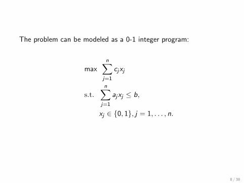
The problem can be modeled as a 0-1 integer program:
maxn∑
j=1
cjxj
s.t.n∑
j=1
ajxj ≤ b,
xj ∈ {0, 1}, j = 1, . . . , n.
8 / 38
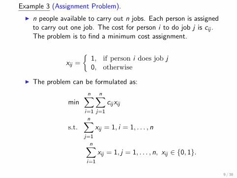
Example 3 (Assignment Problem).
I n people available to carry out n jobs. Each person is assignedto carry out one job. The cost for person i to do job j is cij .The problem is to find a minimum cost assignment.
xij =
{1, if person i does job j0, otherwise
I The problem can be formulated as:
minn∑
i=1
n∑
j=1
cijxij
s.t.n∑
j=1
xij = 1, i = 1, . . . , n
n∑
i=1
xij = 1, j = 1, . . . , n, xij ∈ {0, 1}.
9 / 38
Some Real-World Optimization Problems
I Train scheduling
I Airline crew scheduling
I Highway pavement maintenance and rehabilitation
I Production planing
I Electricity generation planning
I Telecommunications
I Cutting problem
10 / 38
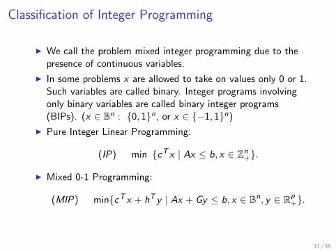
Classification of Integer Programming
I We call the problem mixed integer programming due to thepresence of continuous variables.
I In some problems x are allowed to take on values only 0 or 1.Such variables are called binary. Integer programs involvingonly binary variables are called binary integer programs(BIPs). (x ∈ Bn : {0, 1}n, or x ∈ {−1, 1}n)
I Pure Integer Linear Programming:
(IP) min {cT x | Ax ≤ b, x ∈ Zn+}.
I Mixed 0-1 Programming:
(MIP) min{cT x + hT y | Ax + Gy ≤ b, x ∈ Bn, y ∈ Rp+}.
11 / 38
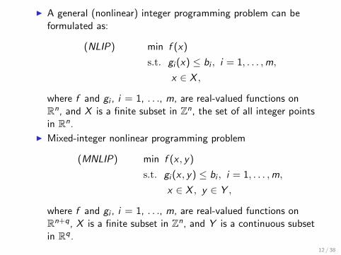
I A general (nonlinear) integer programming problem can beformulated as:
(NLIP) min f (x)
s.t. gi (x) ≤ bi , i = 1, . . . ,m,
x ∈ X ,
where f and gi , i = 1, . . ., m, are real-valued functions onRn, and X is a finite subset in Zn, the set of all integer pointsin Rn.
I Mixed-integer nonlinear programming problem
(MNLIP) min f (x , y)
s.t. gi (x , y) ≤ bi , i = 1, . . . ,m,
x ∈ X , y ∈ Y ,
where f and gi , i = 1, . . ., m, are real-valued functions onRn+q, X is a finite subset in Zn, and Y is a continuous subsetin Rq.
12 / 38
How Hard is Integer Programming?
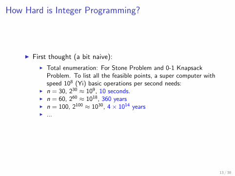
I First thought (a bit naive):
I Total enumeration: For Stone Problem and 0-1 KnapsackProblem. To list all the feasible points, a super computer withspeed 108 (Yi) basic operations per second needs:
I n = 30, 230 ≈ 109, 10 seconds.I n = 60, 260 ≈ 1018, 360 yearsI n = 100, 2100 ≈ 1030, 4× 10¹⁴ yearsI ...
13 / 38
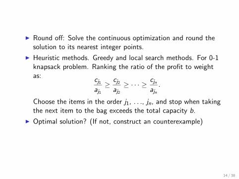
I Round off: Solve the continuous optimization and round thesolution to its nearest integer points.
I Heuristic methods. Greedy and local search methods. For 0-1knapsack problem. Ranking the ratio of the profit to weightas:
cj1
aj1
≥ cj2
aj2
≥ · · · ≥ cjn
ajn
.
Choose the items in the order j1, . . ., jn, and stop when takingthe next item to the bag exceeds the total capacity b.
I Optimal solution? (If not, construct an counterexample)
14 / 38
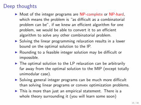
Deep thoughts
I Most of the integer programs are NP-complete or NP-hard,which means the problem is “as difficult as a combinatorialproblem can be”, if we knew an efficient algorithm for oneproblem, we would be able to convert it to an efficientalgorithm to solve any other combinatorial problem.
I Solving the linear programming relaxation results in a lowerbound on the optimal solution to the IP.
I Rounding to a feasible integer solution may be difficult orimpossible.
I The optimal solution to the LP relaxation can be arbitrarilyfar away from the optimal solution to the MIP (except totallyunimodular case).
I Solving general integer programs can be much more difficultthan solving linear programs or convex optimization problems.
I This is more than just an empirical statement. There is awhole theory surrounding it (you will learn some soon)
15 / 38
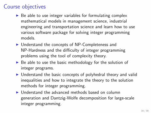
Course objectives
I Be able to use integer variables for formulating complexmathematical models in management science, industrialengineering and transportation science and learn how to usevarious software package for solving integer programmingmodels.
I Understand the concepts of NP-Completeness andNP-Hardness and the difficulty of integer programmingproblems using the tool of complexity theory.
I Be able to use the basic methodology for the solution ofinteger programs.
I Understand the basic concepts of polyhedral theory and validinequalities and how to integrate the theory to the solutionmethods for integer programming.
I Understand the advanced methods based on columngeneration and Dantzig-Wolfe decomposition for large-scaleinteger programming.
16 / 38
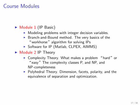
Course Modules
I Module 1 (IP Basic)I Modeling problems with integer decision variables.I Branch-and-Bound method. The very basics of the“workhorse”algorithm for solving IPs
I Software for IP (Matlab, CLPEX, AIMMS)
I Module 2 IP TheoryI Complexity Theory. What makes a problem “hard”or“easy”The complexity classes P, and NP, andNP-completeness
I Polyhedral Theory. Dimension, facets, polarity, and theequivalence of separation and optimization.
17 / 38
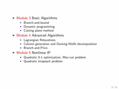
I Module 3 Basic AlgorithmsI Branch-and-boundI Dynamic programmingI Cutting plane method
I Module 4 Advanced AlgorithmsI Lagrangian RelaxationsI Column generation and Dantzig-Wolfe decompositionI Branch-and-Price.
I Module 5 Nonlinear IPI Quadratic 0-1 optimization, Max-cut problemI Quadratic knapsack problem
18 / 38
Combinatorial Optimization Problems
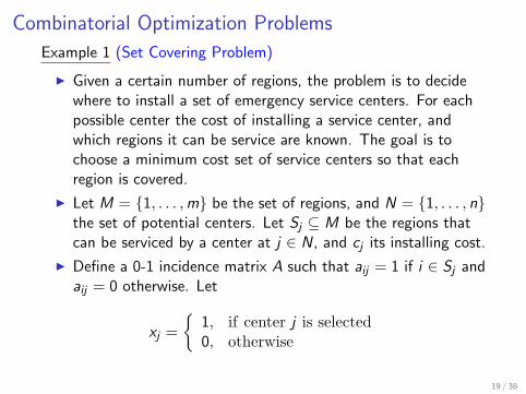
Example 1 (Set Covering Problem)
I Given a certain number of regions, the problem is to decidewhere to install a set of emergency service centers. For eachpossible center the cost of installing a service center, andwhich regions it can be service are known. The goal is tochoose a minimum cost set of service centers so that eachregion is covered.
I Let M = {1, . . . ,m} be the set of regions, and N = {1, . . . , n}the set of potential centers. Let Sj ⊆ M be the regions thatcan be serviced by a center at j ∈ N, and cj its installing cost.
I Define a 0-1 incidence matrix A such that aij = 1 if i ∈ Sj andaij = 0 otherwise. Let
xj =
{1, if center j is selected0, otherwise
19 / 38
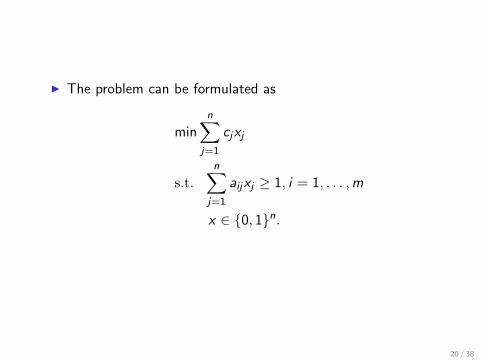
I The problem can be formulated as
minn∑
j=1
cjxj
s.t.n∑
j=1
aijxj ≥ 1, i = 1, . . . ,m
x ∈ {0, 1}n.
20 / 38
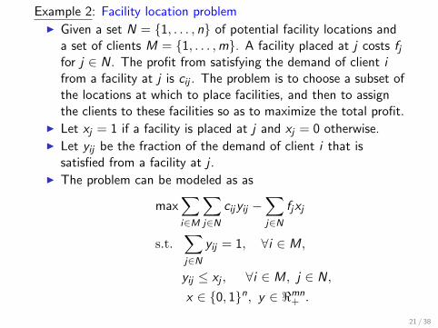
Example 2: Facility location problemI Given a set N = {1, . . . , n} of potential facility locations and
a set of clients M = {1, . . . ,m}. A facility placed at j costs fjfor j ∈ N. The profit from satisfying the demand of client ifrom a facility at j is cij . The problem is to choose a subset ofthe locations at which to place facilities, and then to assignthe clients to these facilities so as to maximize the total profit.
I Let xj = 1 if a facility is placed at j and xj = 0 otherwise.I Let yij be the fraction of the demand of client i that is
satisfied from a facility at j .I The problem can be modeled as as
max∑
i∈M
∑
j∈N
cijyij −∑
j∈N
fjxj
s.t.∑
j∈N
yij = 1, ∀i ∈ M,
yij ≤ xj , ∀i ∈ M, j ∈ N,
x ∈ {0, 1}n, y ∈ <mn+ .
21 / 38
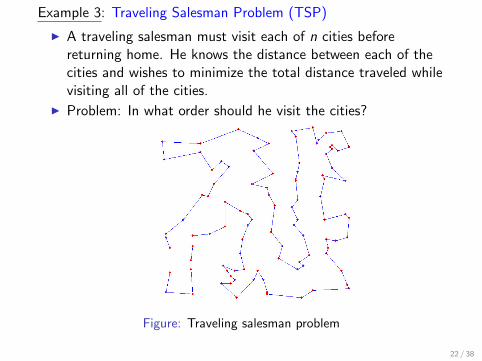
Example 3: Traveling Salesman Problem (TSP)
I A traveling salesman must visit each of n cities beforereturning home. He knows the distance between each of thecities and wishes to minimize the total distance traveled whilevisiting all of the cities.
I Problem: In what order should he visit the cities?
Figure: Traveling salesman problem
22 / 38
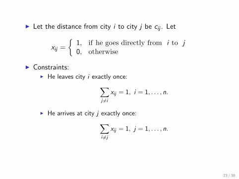
I Let the distance from city i to city j be cij . Let
xij =
{1, if he goes directly from i to j0, otherwise
I Constraints:I He leaves city i exactly once:
∑
j 6=i
xij = 1, i = 1, . . . , n.
I He arrives at city j exactly once:
∑
i 6=j
xij = 1, j = 1, . . . , n.
23 / 38
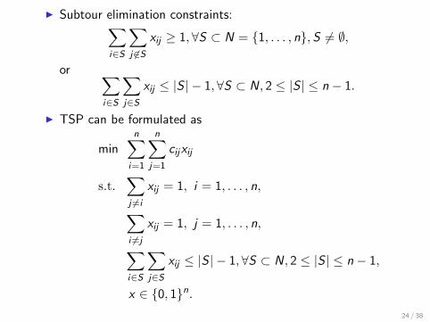
I Subtour elimination constraints:∑
i∈S
∑
j 6∈S
xij ≥ 1,∀S ⊂ N = {1, . . . , n},S 6= ∅,
or ∑
i∈S
∑
j∈S
xij ≤ |S | − 1,∀S ⊂ N, 2 ≤ |S | ≤ n − 1.
I TSP can be formulated as
minn∑
i=1
n∑
j=1
cijxij
s.t.∑
j 6=i
xij = 1, i = 1, . . . , n,
∑
i 6=j
xij = 1, j = 1, . . . , n,
∑
i∈S
∑
j∈S
xij ≤ |S | − 1,∀S ⊂ N, 2 ≤ |S | ≤ n − 1,
x ∈ {0, 1}n.
24 / 38
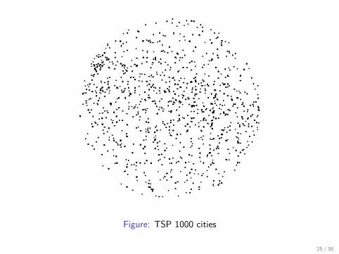
Figure: TSP 1000 cities
25 / 38
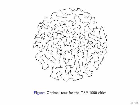
Figure: Optimal tour for the TSP 1000 cities
26 / 38
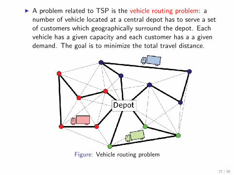
I A problem related to TSP is the vehicle routing problem: anumber of vehicle located at a central depot has to serve a setof customers which geographically surround the depot. Eachvehicle has a given capacity and each customer has a a givendemand. The goal is to minimize the total travel distance.
Figure: Vehicle routing problem
27 / 38
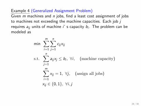
Example 4 (Generalized Assignment Problem)Given m machines and n jobs, find a least cost assignment of jobsto machines not exceeding the machine capacities. Each job jrequires aij units of machine i ’ s capacity bi . The problem can bemodeled as
minm∑
i=1
n∑
j=1
cijxij
s.t.n∑
j=1
aijxj ≤ bi , ∀i , (machine capacity)
m∑
i=1
xij = 1, ∀j , (assign all jobs)
xij ∈ {0, 1}, ∀i , j
28 / 38
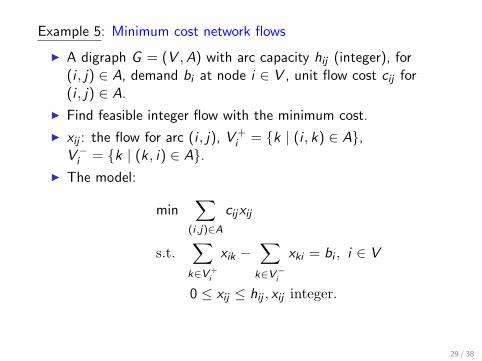
Example 5: Minimum cost network flows
I A digraph G = (V ,A) with arc capacity hij (integer), for(i , j) ∈ A, demand bi at node i ∈ V , unit flow cost cij for(i , j) ∈ A.
I Find feasible integer flow with the minimum cost.
I xij : the flow for arc (i , j), V +i = {k | (i , k) ∈ A},
V−i = {k | (k, i) ∈ A}.
I The model:
min∑
(i ,j)∈A
cijxij
s.t.∑
k∈V +i
xik −∑
k∈V−i
xki = bi , i ∈ V
0 ≤ xij ≤ hij , xij integer.
29 / 38
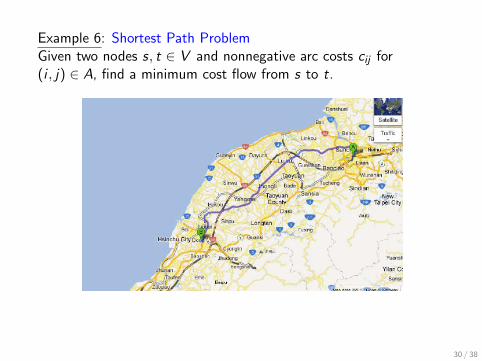
Example 6: Shortest Path ProblemGiven two nodes s, t ∈ V and nonnegative arc costs cij for(i , j) ∈ A, find a minimum cost flow from s to t.
30 / 38
The problem can be formulated as
min∑
(i ,j)∈A
cijxij
s.t.∑
k∈V +i
xik −∑
k∈V−i
xki = 1, i = s
∑
k∈V +i
xik −∑
k∈V−i
xki = 0, i ∈ V \ {s, t}
∑
k∈V +i
xik −∑
k∈V−i
xki = −1, i = t
xij ∈ {0, 1}, (i , j) ∈ A.
31 / 38
Example 7: Maximum flow problem
I Given two nodes s, t ∈ V and nonnegative arc capacities hij
for (i , j) ∈ A, find a maximum flow from s to t.
I Adding a backward arc from t to s with hij = +∞. TheMaximum flow problem can be formulated as
max xts
s.t.∑
k∈V +i
xik −∑
k∈V−i
xki = 0, i ∈ V ,
0 ≤ xij ≤ hij , (i , j) ∈ A.
32 / 38
Nonlinear Integer Programming Models
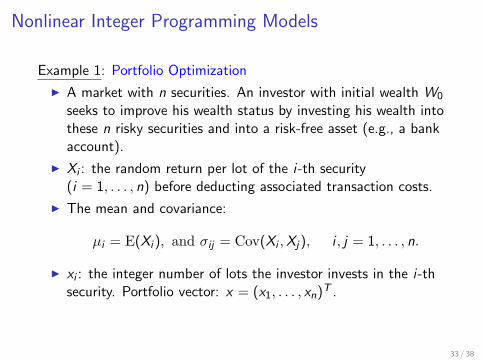
Example 1: Portfolio Optimization
I A market with n securities. An investor with initial wealth W0
seeks to improve his wealth status by investing his wealth intothese n risky securities and into a risk-free asset (e.g., a bankaccount).
I Xi : the random return per lot of the i-th security(i = 1, . . . , n) before deducting associated transaction costs.
I The mean and covariance:
µi = E(Xi ), and σij = Cov(Xi ,Xj), i , j = 1, . . . , n.
I xi : the integer number of lots the investor invests in the i-thsecurity. Portfolio vector: x = (x1, . . . , xn)
T .
33 / 38
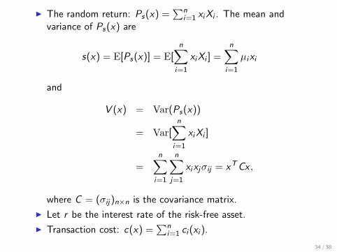
I The random return: Ps(x) =∑n
i=1 xiXi . The mean andvariance of Ps(x) are
s(x) = E[Ps(x)] = E[n∑
i=1
xiXi ] =n∑
i=1
µixi
and
V (x) = Var(Ps(x))
= Var[n∑
i=1
xiXi ]
=n∑
i=1
n∑
j=1
xixjσij = xTCx ,
where C = (σij)n×n is the covariance matrix.
I Let r be the interest rate of the risk-free asset.
I Transaction cost: c(x) =∑n
i=1 ci (xi ).
34 / 38
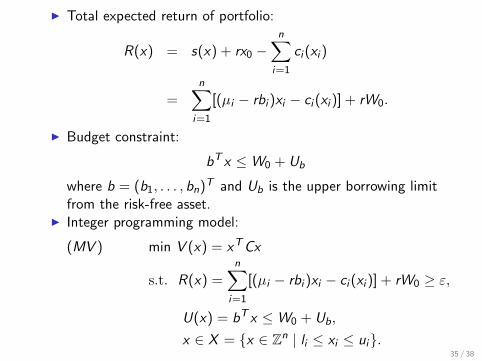
I Total expected return of portfolio:
R(x) = s(x) + rx0 −n∑
i=1
ci (xi )
=n∑
i=1
[(µi − rbi )xi − ci (xi )] + rW0.
I Budget constraint:
bT x ≤ W0 + Ub
where b = (b1, . . . , bn)T and Ub is the upper borrowing limit
from the risk-free asset.I Integer programming model:
(MV ) min V (x) = xTCx
s.t. R(x) =n∑
i=1
[(µi − rbi )xi − ci (xi )] + rW0 ≥ ε,
U(x) = bT x ≤ W0 + Ub,
x ∈ X = {x ∈ Zn | li ≤ xi ≤ ui}.35 / 38
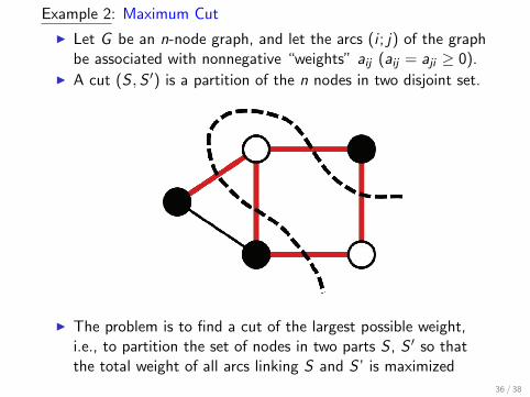
Example 2: Maximum Cut
I Let G be an n-node graph, and let the arcs (i ; j) of the graphbe associated with nonnegative “weights” aij (aij = aji ≥ 0).
I A cut (S ,S ′) is a partition of the n nodes in two disjoint set.
I The problem is to find a cut of the largest possible weight,i.e., to partition the set of nodes in two parts S , S ′ so thatthe total weight of all arcs linking S and S ’ is maximized
36 / 38
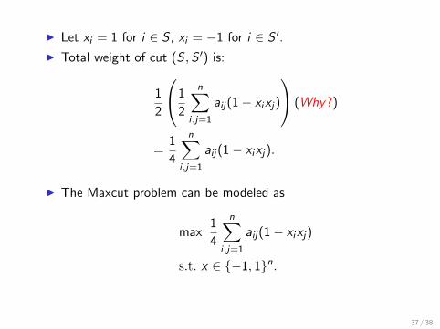
I Let xi = 1 for i ∈ S , xi = −1 for i ∈ S ′.I Total weight of cut (S ,S ′) is:
1
2
1
2
n∑
i ,j=1
aij(1− xixj)
(Why?)
=1
4
n∑
i ,j=1
aij(1− xixj).
I The Maxcut problem can be modeled as
max1
4
n∑
i ,j=1
aij(1− xixj)
s.t. x ∈ {−1, 1}n.
37 / 38
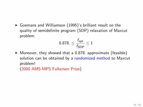
I Goemans and Williamson (1995)’s brilliant result on thequality of semidefinite program (SDP) relaxation of Maxcutproblem:
0.878. ≤ fopt
fSDP≤ 1
I Moreover, they showed that a 0.878. approximate (feasible)solution can be obtained by a randomized method to Maxcutproblem!(2000 AMS-MPS Fulkerson Prize)
38 / 38
Recommended