Interactive CurveModelingwith Applications to Computer Graphics,Vision and Image Processing
Muhammad Sarfraz
13
| | | | | | | | | | | | | | | | | | | | | | | | | | | | | | | | | | | | | |
| | | | | | | | | | | | | | | | | | | | | | | | | | | | | | | | | | | | | | |
| | | | | | | | | | | | | | | | | | | | | | | | | | | | | | | | | |
| | | | | | | | | | | | | | | | | | | | | | | | | | | | | | | | | | | | | | | | | | |
| | | | | | | | | | | | | | | | | | | | | | | | | | | | | | | |

Interactive Curve Modeling

M. Sarfraz
Interactive Curve Modeling
and Image Processingith Applications to Computer Graphics,
VisionW

M. Sarfraz, BSc, MSc, MSc, PhdDepartment of Information ScienceKuwait UniversitySafat, Kuwait
and
Department of Information and Computer ScienceKing Fahd University of Petroleum and MineralsDhahran, Saudi Arabia
British Library Cataloguing in Publication DataA catalogue record for this book is available from the British Library
Library of Congress Control Number: 2007926244
Printed on acid-free paper
ISBN 978-1-84628-870-8 e-ISBN 978-1-84628-871-5
c© Springer-Verlag London Limited 2008Apart from any fair dealing for the purposes of research or private study, or criticism or review, aspermitted under the Copyright, Designs and Patents Act 1988, this publication may only be reproduced,stored or transmitted, in any form or by any means, with the prior permission in writing of the publishers,or in the case of reprographic reproduction in accordance with the terms of licences issued by theCopyright Licensing Agency. Enquiries concerning reproduction outside those terms should be sent tothe publishers.
The use of registered names, trademarks, etc. in this publication does not imply, even in the absence ofa specific statement, that such names are exempt from the relevant laws and regulations and thereforefree for general use.
The publisher makes no representation, express or implied, with regard to the accuracy of the infor-mation contained in this book and cannot accept any legal responsibility or liability for any errors oromissions that may be made.
9 8 7 6 5 4 3 2 1
Springer Science+Business Mediaspringer.com

To the major contributors to my life:
My primary school teacher M. Aslam
My friends Ashfaq and Abid
My father in memoriam
My mother
My wife
My children Ihsan, Humaira, Inam, and Ikram
Interactive curve modeling techniques and their applications are extremely usefulin a number of academic and industrial settings. Specifically, curve modeling playsa significant role in multidisciplinary problem solving. It is extremely useful invarious situations like font design, designing objects, CAD/CAM, medical imag-ing and visualization, scientific data visualization, virtual reality, object recogni-tion, etc. In particular, various problems like iris recognition, fingerprint recog-nition, signature recognition, etc. can also be intelligently solved and automatedusing curve techniques. In addition to its critical importance more recently, thecurve modeling methods have also proven to be indispensable in a variety of mod-ern industries, including computer vision, robotics, medical imaging, visualiza-tion, and even media.
This book aims to provide a valuable source that focuses on interdisciplinarymethods and to add up-to-date methodologies in the area. It aims to provide theuser community with a variety of techniques, applications, and systems necessaryfor various real-life problems in the areas such as font design, medical visualiza-tion, scientific data visualization, archaeology, toon rendering, virtual reality, bodysimulation, outline capture of images, object recognition, signature recognition,industrial applications, and many others.
Book Features
It aims to collect and disseminate information in various disciplines includingcomputer graphics, image processing, computer vision, pattern recognition, artifi-cial intelligence, soft computing, shape analysis and description, curve and surfacefitting, scientific visualization, shape abstraction and modeling, intelligent CADsystems, computational geometry, reverse engineering, and levels of details forcurves and surfaces. The major goal of this book is to stimulate views and providea source where students, researchers, and practitioners can find the latest devel-opments in the field of interactive curve modeling and its applications. The bookprovides classical and up-to-date theory and practice to get the problems solved indiverse areas of science and engineering.
All the chapters of the book will contribute toward curve modeling techniques,applications, and systems. The book will have the best possible utility for stu-dents, researchers, computer scientists, practicing engineers, and many others whoseek classical and state-of-the-art techniques, applications, and systems with curve
vii
Preface
viii Preface
modeling. It will be an extremely useful book for undergraduate senior students aswell as graduate students in the areas of computer science, engineering, and othercomputational sciences.
Suggested Course Outlines
This book is designed to have around fifteen chapters. These chapters will con-tribute toward interactive curve modeling techniques, applications, systems, andtools. The book is planned to have the best possible utility for researchers, com-puter scientists, practicing engineers, and many others who seek classical andstate-of-the-art techniques and applications for computer graphics, vision, andimaging. It will also be equally and extremely useful for undergraduate seniorstudents as well as graduate students in the areas of computer science. It is alsobeneficial to students in other disciplines including computer engineering, electri-cal engineering, mechanical engineering, and mathematics. The book is equallybeneficial to researchers and practitioners in the industry and academia.
The book has been designed as a course book for undergraduate as well as grad-uate students in the area of computer science in particular. The main audience ofthe book are the communities related to the field of computer graphics, vision,and imaging. However, it can be useful for students in other disciplines like com-puter engineering, electrical engineering, mechanical engineering, mathematics,etc. The book is equally beneficial to researchers and practitioners in the industry.The book can formulate at least three courses as follows:
Course I. As an undergraduate course, at senior level, Chaps. 1–3, 8, 9, 11 (anytwo corner detectors), 12 (any two methods), 13, and 14 (one heuristicapproach) will comprise a full length three credit hours course for a semesterof 15 weeks. This course can be conducted with practical projects of reason-able weight.
Course II. As a graduate course consisting of Chaps. 1–4, 6–8 (self-study), 9, and11–14 (one heuristic approach). This course should also have heavy projectsfor practical applications.
Course III. As a slightly different graduate course, if the undergraduate coursedescribed in Course I is considered to be a prerequisite. This course can bedesigned with Chaps. 4–7, 9 (using other curve schemes in the book butdifferent than those in Chap. 9), 11–13 (just a quick review), 14, and 15.This course design can also consist of some state-of-the-art topics togetherwith good weighted projects.
The researchers and practitioners can utilize the manuscript as a source as wellas a reference book. Depending on their needs, they can study on pick and choosebasis. They are also advised to study in their leisure time as it may prove to befruitful to them.

Preface ix
Required Background
As such, it is not required to possess a specific qualification as a prerequisite to anyof the undergraduate Course I or graduate courses II or III mentioned above. But,the user of this book is presumed to have some knowledge of computer program-ming together with some basic mathematical topics including analytic geometry,linear algebra, and calculus.
Acknowledgments
This manuscript has been prepared after a lot of struggle and efforts. Many gradu-ate students and colleagues around the globe have assisted toward its completion.It is worthwhile to mention Asif Masood, Zulfiqar Habib, M. Zawwar Hussain,S. Ali Rizvi, M. Balah, M. Riyazuddin, Humayun Baig, S. Arshad Raza, MurtazaAli Khan, Faisal AbdulRazzak, and M.A. Siddiqui. The author is thankful to allof them for their valuable efforts and advice. A lot of credit is also due to variousexperts who reviewed the chapters and provided helpful feedback.
It is not possible to forget my family here without whose help and supportI would not have completed this work. Their love, support, and patience weretremendous throughout. In addition to thanking, I should also apologize for hav-ing taken much of their time during the conduct of my work.
The author is happy to acknowledge the support of King Fahd University ofPetroleum and Minerals (KFUPM) toward the compilation of this book, againstthe Book Project #ICS/GRAPHICS/306. This book project was a main sourceof funding to this book. A partial funded support of KFUPM, through anotherResearch Project #ICS/REVERSE ENG./312, also contributed toward a couple ofchapters.
M. Sarfraz
Contents
Preface . . . . . . . . . . . . . . . . . . . . . . . . . . . . . . . . . . . . . vii
1 Introduction . . . . . . . . . . . . . . . . . . . . . . . . . . . . . . . . 11.1 Strategy in the Construction of Theory . . . . . . . . . . . . . . 11.2 Overview . . . . . . . . . . . . . . . . . . . . . . . . . . . . . 2
1.2.1 Splines . . . . . . . . . . . . . . . . . . . . . . . . . . 21.2.2 Shape-Preserving Interpolation . . . . . . . . . . . . . . 31.2.3 Functional Approximation . . . . . . . . . . . . . . . . 31.2.4 Spiral Curves . . . . . . . . . . . . . . . . . . . . . . . 41.2.5 Corner Detection and Curve Segmentation . . . . . . . . 41.2.6 Vectorizing Planar Shapes . . . . . . . . . . . . . . . . 51.2.7 Reverse Engineering . . . . . . . . . . . . . . . . . . . 51.2.8 Multiresolution Framework . . . . . . . . . . . . . . . . 6
1.3 Notation and Conventions . . . . . . . . . . . . . . . . . . . . . 61.4 Review of Some Spline Methods . . . . . . . . . . . . . . . . . 7
1.4.1 Cubic Spline . . . . . . . . . . . . . . . . . . . . . . . 71.4.2 Spline Under Tension . . . . . . . . . . . . . . . . . . . 81.4.3 Weighted Spline . . . . . . . . . . . . . . . . . . . . . 81.4.4 Nu-spline . . . . . . . . . . . . . . . . . . . . . . . . . 81.4.5 Weighted Nu-spline . . . . . . . . . . . . . . . . . . . . 91.4.6 Beta Splines . . . . . . . . . . . . . . . . . . . . . . . . 91.4.7 Sigma (σ) Splines . . . . . . . . . . . . . . . . . . . . 101.4.8 B-Splines . . . . . . . . . . . . . . . . . . . . . . . . . 101.4.9 Bezier Splines . . . . . . . . . . . . . . . . . . . . . . 111.4.10 Hermite Splines . . . . . . . . . . . . . . . . . . . . . . 11
1.5 Summary . . . . . . . . . . . . . . . . . . . . . . . . . . . . . 131.6 Exercises . . . . . . . . . . . . . . . . . . . . . . . . . . . . . 13
2 Weighted Nu Splines . . . . . . . . . . . . . . . . . . . . . . . . . . . 212.1 Introduction . . . . . . . . . . . . . . . . . . . . . . . . . . . . 212.2 Some Spline Methods . . . . . . . . . . . . . . . . . . . . . . . 23
2.2.1 Cubic Splines . . . . . . . . . . . . . . . . . . . . . . . 242.2.2 Weighted Splines . . . . . . . . . . . . . . . . . . . . . 242.2.3 Nu Splines . . . . . . . . . . . . . . . . . . . . . . . . 26
xi
xii Contents
2.2.4 Weighted Nu Splines . . . . . . . . . . . . . . . . . . . 272.2.5 Demonstration . . . . . . . . . . . . . . . . . . . . . . 28
2.3 Freeform Weighted Nu Spline . . . . . . . . . . . . . . . . . . 282.3.1 Local Support Basis . . . . . . . . . . . . . . . . . . . 292.3.2 Design Curve . . . . . . . . . . . . . . . . . . . . . . . 312.3.3 Shape Control . . . . . . . . . . . . . . . . . . . . . . . 322.3.4 Demonstration . . . . . . . . . . . . . . . . . . . . . . 342.3.5 Advantages and Features . . . . . . . . . . . . . . . . . 37
2.4 Surfaces . . . . . . . . . . . . . . . . . . . . . . . . . . . . . . 372.5 Summary . . . . . . . . . . . . . . . . . . . . . . . . . . . . . 382.6 Exercises . . . . . . . . . . . . . . . . . . . . . . . . . . . . . 38
3 Rational Cubic Spline with Shape Control . . . . . . . . . . . . . . . . 413.1 Introduction . . . . . . . . . . . . . . . . . . . . . . . . . . . . 413.2 C1 Piecewise Rational Cubic Hermite Interpolant . . . . . . . . 423.3 One-Parameter Rational Cubic Spline . . . . . . . . . . . . . . 443.4 Two-Parameter Rational Cubic Spline . . . . . . . . . . . . . . 493.5 Demonstration . . . . . . . . . . . . . . . . . . . . . . . . . . . 513.6 Freeform Curves . . . . . . . . . . . . . . . . . . . . . . . . . 553.7 Local Support Basis . . . . . . . . . . . . . . . . . . . . . . . . 563.8 Design Curve . . . . . . . . . . . . . . . . . . . . . . . . . . . 583.9 Shape Properties . . . . . . . . . . . . . . . . . . . . . . . . . . 603.10 Demonstration . . . . . . . . . . . . . . . . . . . . . . . . . . . 643.11 Nurbs . . . . . . . . . . . . . . . . . . . . . . . . . . . . . . . 643.12 Surfaces . . . . . . . . . . . . . . . . . . . . . . . . . . . . . . 703.13 Summary . . . . . . . . . . . . . . . . . . . . . . . . . . . . . 713.14 Exercises . . . . . . . . . . . . . . . . . . . . . . . . . . . . . 71
4 Rational Sigma (σ ) Splines . . . . . . . . . . . . . . . . . . . . . . . . 754.1 Introduction . . . . . . . . . . . . . . . . . . . . . . . . . . . . 754.2 Generalized Rational Cubic Interpolant . . . . . . . . . . . . . . 764.3 Interpolatory Rational σ -Splines . . . . . . . . . . . . . . . . . 77
4.3.1 Shape Control . . . . . . . . . . . . . . . . . . . . . . . 774.3.2 Some Special Cases . . . . . . . . . . . . . . . . . . . 784.3.3 Examples . . . . . . . . . . . . . . . . . . . . . . . . . 78
4.4 Freeform Rational σ -Splines . . . . . . . . . . . . . . . . . . . 814.4.1 Shape Control . . . . . . . . . . . . . . . . . . . . . . . 844.4.2 Some Special Cases . . . . . . . . . . . . . . . . . . . 854.4.3 Examples . . . . . . . . . . . . . . . . . . . . . . . . . 87
4.5 Exercises . . . . . . . . . . . . . . . . . . . . . . . . . . . . . 91
5 Linear, Conic and Rational Cubic Splines . . . . . . . . . . . . . . . . 935.1 Introduction . . . . . . . . . . . . . . . . . . . . . . . . . . . . 935.2 The Rational Cubic Spline . . . . . . . . . . . . . . . . . . . . 95
5.2.1 Estimation of Tangent Vectors . . . . . . . . . . . . . . 97
Contents xiii
5.3 Design Curve Analysis . . . . . . . . . . . . . . . . . . . . . . 995.4 Estimation of End Tangent Vectors . . . . . . . . . . . . . . . . 1015.5 Conic Splines and Straight Line . . . . . . . . . . . . . . . . . 101
5.5.1 Conic Arc in Cubic Spline . . . . . . . . . . . . . . . . 1035.5.2 Circular Spline . . . . . . . . . . . . . . . . . . . . . . 1035.5.3 Circular Arc . . . . . . . . . . . . . . . . . . . . . . . . 105
5.5.3.1 Circular Arc for Given Radius . . . . . . . . . . 1065.5.3.2 Circular Arc for a Given Center . . . . . . . . . 106
5.5.4 Elliptic Arc . . . . . . . . . . . . . . . . . . . . . . . . 1075.5.5 Intermediate Point Interpolation . . . . . . . . . . . . . 1095.5.6 Straight-Line Segment . . . . . . . . . . . . . . . . . . 110
5.6 Examples . . . . . . . . . . . . . . . . . . . . . . . . . . . . . 1105.7 Summary . . . . . . . . . . . . . . . . . . . . . . . . . . . . . 1135.8 Exercises . . . . . . . . . . . . . . . . . . . . . . . . . . . . . 113
6 Shape-Preserving Rational Interpolation for Planar Curves . . . . . . . 1176.1 Introduction . . . . . . . . . . . . . . . . . . . . . . . . . . . . 1176.2 The Rational Cubic Interpolant . . . . . . . . . . . . . . . . . . 1186.3 Interpolation of Convex Data . . . . . . . . . . . . . . . . . . . 1196.4 Interpolation of Monotonic Data . . . . . . . . . . . . . . . . . 1206.5 Interpolation of Convex and Monotonic Data . . . . . . . . . . 1236.6 Choice of Tangent Vectors . . . . . . . . . . . . . . . . . . . . 1236.7 Examples . . . . . . . . . . . . . . . . . . . . . . . . . . . . . 1246.8 Summary . . . . . . . . . . . . . . . . . . . . . . . . . . . . . 1266.9 Exercises . . . . . . . . . . . . . . . . . . . . . . . . . . . . . 126
7 Visualization of Shaped Data by a Rational Cubic Spline . . . . . . . . 1297.1 Introduction . . . . . . . . . . . . . . . . . . . . . . . . . . . . 1297.2 Rational Cubic Spline with Shape Control . . . . . . . . . . . . 133
7.2.1 Shape Control Analysis . . . . . . . . . . . . . . . . . . 1347.2.2 Determination of Derivatives . . . . . . . . . . . . . . . 135
7.2.2.1 Derivative Method I . . . . . . . . . . . . . . . 1357.2.2.2 Derivative Method II . . . . . . . . . . . . . . 1357.2.2.3 Derivative Method III . . . . . . . . . . . . . . 136
7.2.3 Examples and Discussion . . . . . . . . . . . . . . . . . 1367.3 Positive Spline Interpolation . . . . . . . . . . . . . . . . . . . 139
7.3.1 Examples and Discussion . . . . . . . . . . . . . . . . . 1427.4 Monotone Spline Interpolation . . . . . . . . . . . . . . . . . . 145
7.4.1 Examples and Discussion . . . . . . . . . . . . . . . . . 1487.5 Convex Spline Interpolation . . . . . . . . . . . . . . . . . . . 148
7.5.1 Demonstration . . . . . . . . . . . . . . . . . . . . . . 1537.6 Summary . . . . . . . . . . . . . . . . . . . . . . . . . . . . . 1547.7 Exercises . . . . . . . . . . . . . . . . . . . . . . . . . . . . . 154
8 Visualization of Shaped Data by Cubic Spline Interpolation . . . . . . . 1578.1 Introduction . . . . . . . . . . . . . . . . . . . . . . . . . . . . 157
xiv Contents
8.2 Cubic Interpolant . . . . . . . . . . . . . . . . . . . . . . . . . 1588.2.1 Demonstration . . . . . . . . . . . . . . . . . . . . . . 159
8.3 Shape-Preserving Interpolation . . . . . . . . . . . . . . . . . . 1608.4 Convex Cubic Spline . . . . . . . . . . . . . . . . . . . . . . . 160
8.4.1 Demonstration . . . . . . . . . . . . . . . . . . . . . . 1628.5 Monotone Cubic Spline . . . . . . . . . . . . . . . . . . . . . . 162
8.5.1 Demonstration . . . . . . . . . . . . . . . . . . . . . . 1648.6 Positive Cubic Spline . . . . . . . . . . . . . . . . . . . . . . . 164
8.6.1 Demonstration . . . . . . . . . . . . . . . . . . . . . . 1668.7 Extension of Positive Cubic Spline . . . . . . . . . . . . . . . . 167
8.7.1 Demonstration . . . . . . . . . . . . . . . . . . . . . . 1708.8 Summary . . . . . . . . . . . . . . . . . . . . . . . . . . . . . 1718.9 Exercises . . . . . . . . . . . . . . . . . . . . . . . . . . . . . 171
9 Approximation with B-Splines Curves . . . . . . . . . . . . . . . . . . 1739.1 Introduction . . . . . . . . . . . . . . . . . . . . . . . . . . . . 1739.2 B-Splines . . . . . . . . . . . . . . . . . . . . . . . . . . . . . 1749.3 Deterministic Approach . . . . . . . . . . . . . . . . . . . . . . 174
9.3.1 Approximation Technique . . . . . . . . . . . . . . . . 1759.3.1.1 Initial Data Points (Step 1) . . . . . . . . . . . 1759.3.1.2 Knot Insertion (Step 2) . . . . . . . . . . . . . 1779.3.1.3 Error Minimization (Step 3) . . . . . . . . . . . 178
9.3.2 Demonstration . . . . . . . . . . . . . . . . . . . . . . 1789.4 Nondeterministic Approach . . . . . . . . . . . . . . . . . . . . 180
9.4.1 A Brief Overview of GAs . . . . . . . . . . . . . . . . 1819.4.2 Implementation Summary . . . . . . . . . . . . . . . . 1819.4.3 Demonstration . . . . . . . . . . . . . . . . . . . . . . 183
9.5 Summary . . . . . . . . . . . . . . . . . . . . . . . . . . . . . 1939.6 Exercises . . . . . . . . . . . . . . . . . . . . . . . . . . . . . 193
10 Spirals . . . . . . . . . . . . . . . . . . . . . . . . . . . . . . . . . . . 19510.1 Introduction . . . . . . . . . . . . . . . . . . . . . . . . . . . . 19510.2 The Rational Quadratic Bezier Curve . . . . . . . . . . . . . . . 19610.3 The Conic Spiral . . . . . . . . . . . . . . . . . . . . . . . . . 19710.4 Comparison of Conic and T-cubic Spirals . . . . . . . . . . . . 20010.5 The Arc/Conic Spiral . . . . . . . . . . . . . . . . . . . . . . . 20110.6 Examples . . . . . . . . . . . . . . . . . . . . . . . . . . . . . 20510.7 Limitations . . . . . . . . . . . . . . . . . . . . . . . . . . . . 20610.8 Summary . . . . . . . . . . . . . . . . . . . . . . . . . . . . . 20610.9 Exercises . . . . . . . . . . . . . . . . . . . . . . . . . . . . . 206
11 Corner Detection for Curve Segmentation . . . . . . . . . . . . . . . . 20911.1 Introduction . . . . . . . . . . . . . . . . . . . . . . . . . . . . 20911.2 Basic Formulation . . . . . . . . . . . . . . . . . . . . . . . . . 21011.3 Summary of Commonly Referred Corner Detectors . . . . . . . 212
Contents xv
11.3.1 Rosenfeld and Johnston (RJ73) Algorithm . . . . . . . . 21211.3.2 Rosenfeld and Weszka (RW75) Algorithm . . . . . . . . 21311.3.3 Freeman and Davis (FD77) Algorithm . . . . . . . . . . 21311.3.4 Beus and Tiu (BT87) Algorithm . . . . . . . . . . . . . 214
11.4 Chetverikov and Szabo (CS99) Algorithm . . . . . . . . . . . . 21511.4.1 First Pass . . . . . . . . . . . . . . . . . . . . . . . . . 21511.4.2 Second Pass . . . . . . . . . . . . . . . . . . . . . . . . 21611.4.3 Demonstration . . . . . . . . . . . . . . . . . . . . . . 21611.4.4 Performance Evaluation . . . . . . . . . . . . . . . . . 218
11.5 Sarfraz, Asim and Masood (SAM06) Algorithm . . . . . . . . . 21911.5.1 First Pass . . . . . . . . . . . . . . . . . . . . . . . . . 21911.5.2 Second Pass . . . . . . . . . . . . . . . . . . . . . . . . 22011.5.3 Parameters . . . . . . . . . . . . . . . . . . . . . . . . 22111.5.4 Demonstration . . . . . . . . . . . . . . . . . . . . . . 221
11.6 Masood and Sarfraz (MS06) Algorithm . . . . . . . . . . . . . 22611.6.1 Performance Criteria . . . . . . . . . . . . . . . . . . . 23011.6.2 Demonstration . . . . . . . . . . . . . . . . . . . . . . 231
11.7 Overall Analysis . . . . . . . . . . . . . . . . . . . . . . . . . . 23511.8 Piecing Boundaries . . . . . . . . . . . . . . . . . . . . . . . . 23611.9 Summary . . . . . . . . . . . . . . . . . . . . . . . . . . . . . 23711.10 Exercises . . . . . . . . . . . . . . . . . . . . . . . . . . . . . 238
12 Linear Capture of Digital Curves . . . . . . . . . . . . . . . . . . . . . 24112.1 Introduction . . . . . . . . . . . . . . . . . . . . . . . . . . . . 24112.2 Some Important Issues . . . . . . . . . . . . . . . . . . . . . . 243
12.2.1 Input Parameters . . . . . . . . . . . . . . . . . . . . . 24312.2.2 Region of Support . . . . . . . . . . . . . . . . . . . . 24412.2.3 Error Measurement . . . . . . . . . . . . . . . . . . . . 24412.2.4 Min-# and Min-ε Problems . . . . . . . . . . . . . . . . 24512.2.5 Test Shapes . . . . . . . . . . . . . . . . . . . . . . . . 245
12.3 Approximation Techniques . . . . . . . . . . . . . . . . . . . . 24612.3.1 Teh and Chin Algorithm . . . . . . . . . . . . . . . . . 24712.3.2 Marji and Siy Algorithm . . . . . . . . . . . . . . . . . 24812.3.3 Wu Algorithm . . . . . . . . . . . . . . . . . . . . . . 24912.3.4 Some Other Algorithms . . . . . . . . . . . . . . . . . 250
12.4 Piecewise Polygonal Approximation . . . . . . . . . . . . . . . 25112.4.1 Preprocessing Stage . . . . . . . . . . . . . . . . . . . 25112.4.2 SAMAPA Algorithm . . . . . . . . . . . . . . . . . . . 252
12.5 Experimental Results . . . . . . . . . . . . . . . . . . . . . . . 25612.6 Optimal Algorithms . . . . . . . . . . . . . . . . . . . . . . . . 259
12.6.1 Dynamic Programming . . . . . . . . . . . . . . . . . . 25912.6.2 Perez and Vidal Algorithm . . . . . . . . . . . . . . . . 26012.6.3 Some Remarks on Optimal Algorithms . . . . . . . . . 261
12.7 Summary . . . . . . . . . . . . . . . . . . . . . . . . . . . . . 26212.8 Exercises . . . . . . . . . . . . . . . . . . . . . . . . . . . . . 262
xvi Contents
13 Digital Outline Capture with Cubic Curves . . . . . . . . . . . . . . . . 26713.1 Introduction . . . . . . . . . . . . . . . . . . . . . . . . . . . . 26713.2 Finding the Boundary of a Bitmap Image . . . . . . . . . . . . . 26813.3 Detecting Corner Points . . . . . . . . . . . . . . . . . . . . . . 27013.4 Filtering Noise . . . . . . . . . . . . . . . . . . . . . . . . . . 27113.5 Curve Fitting with Cubic Bezier . . . . . . . . . . . . . . . . . 272
13.5.1 Finding Intermediate Control Points . . . . . . . . . . . 27313.5.2 Comparing the Boundary and Parametric Curve . . . . . 276
13.6 Reparameterization . . . . . . . . . . . . . . . . . . . . . . . . 27613.7 Breaking Segment . . . . . . . . . . . . . . . . . . . . . . . . . 27913.8 Alternate Method Using Hermite Cubic . . . . . . . . . . . . . 281
13.8.1 Estimation of Tangent Vectors . . . . . . . . . . . . . . 28213.8.2 Optimal Design Curve . . . . . . . . . . . . . . . . . . 283
13.9 Transformations and Mapping . . . . . . . . . . . . . . . . . . 28513.9.1 Transformations . . . . . . . . . . . . . . . . . . . . . 28713.9.2 Mapping Parametric Surfaces . . . . . . . . . . . . . . 288
13.9.2.1 Two-Dimensional Surface Mapping . . . . . . . 29013.9.2.2 Three-Dimensional Surface Mapping . . . . . . 293
13.10 Summary . . . . . . . . . . . . . . . . . . . . . . . . . . . . . 29313.11 Exercises . . . . . . . . . . . . . . . . . . . . . . . . . . . . . 293
14 Computer-Aided Reverse Engineering Using Evolutionary Heuristicson NURBS . . . . . . . . . . . . . . . . . . . . . . . . . . . . . . . . 29714.1 Introduction . . . . . . . . . . . . . . . . . . . . . . . . . . . . 29714.2 Preprocessing . . . . . . . . . . . . . . . . . . . . . . . . . . . 299
14.2.1 Image Contour Extraction . . . . . . . . . . . . . . . . 29914.2.2 Detection of Corner Points . . . . . . . . . . . . . . . . 299
14.3 NURBS . . . . . . . . . . . . . . . . . . . . . . . . . . . . . . 30114.3.1 Data Fitting Using NURBS Curves . . . . . . . . . . . 30214.3.2 Generation of Control Points for Curves . . . . . . . . . 30314.3.3 Generation of Control Points for Surfaces . . . . . . . . 304
14.4 Approach Using SimE . . . . . . . . . . . . . . . . . . . . . . 30414.4.1 Outline of SimE . . . . . . . . . . . . . . . . . . . . . 30414.4.2 Problem Mapping SimE . . . . . . . . . . . . . . . . . 304
14.4.2.1 Initialization . . . . . . . . . . . . . . . . . . . 30514.4.2.2 Evaluation . . . . . . . . . . . . . . . . . . . . 30514.4.2.3 Selection . . . . . . . . . . . . . . . . . . . . . 30614.4.2.4 Allocation and Weight Optimization for Curves 306
14.4.3 Algorithm Outline for Curves . . . . . . . . . . . . . . 30614.4.4 Demonstration . . . . . . . . . . . . . . . . . . . . . . 309
14.5 Approach Using SimA . . . . . . . . . . . . . . . . . . . . . . 31214.5.1 Outline of SimE . . . . . . . . . . . . . . . . . . . . . 31314.5.2 Problem Mapping . . . . . . . . . . . . . . . . . . . . . 313
14.5.2.1 Weight Optimization Using SimA . . . . . . . . 31314.5.2.2 Initial Temperature T0 . . . . . . . . . . . . . . 315
Contents xvii
14.5.2.3 Decrement of T . . . . . . . . . . . . . . . . . 31514.5.2.4 Length of Markov Chain M . . . . . . . . . . . 31514.5.2.5 Weight Seclection . . . . . . . . . . . . . . . . 316
14.5.3 Demonstration . . . . . . . . . . . . . . . . . . . . . . 31614.6 Surfaces . . . . . . . . . . . . . . . . . . . . . . . . . . . . . . 32214.7 Summary . . . . . . . . . . . . . . . . . . . . . . . . . . . . . 32814.8 Exercises . . . . . . . . . . . . . . . . . . . . . . . . . . . . . 329
15 Multiresolution Framework for B-Splines . . . . . . . . . . . . . . . . 33115.1 Introduction . . . . . . . . . . . . . . . . . . . . . . . . . . . . 33115.2 Theory of NUBS . . . . . . . . . . . . . . . . . . . . . . . . . 33215.3 Multiresolution Representation of B-Splines . . . . . . . . . . . 333
15.3.1 Multiresolution Representation of B-SplinesUsing Wavelets . . . . . . . . . . . . . . . . . . . . . . 334
15.3.2 Multiresolution of NUBS Using Knot Decimation . . . . 33515.4 Multiresolution of NUBS Using Control Point Decimation . . . 33615.5 Demonstration . . . . . . . . . . . . . . . . . . . . . . . . . . . 33915.6 Summary . . . . . . . . . . . . . . . . . . . . . . . . . . . . . 34115.7 Exercises . . . . . . . . . . . . . . . . . . . . . . . . . . . . . 343
Index . . . . . . . . . . . . . . . . . . . . . . . . . . . . . . . . . . . . . 345
1Introduction
Abstract. Interactive curve designing plays an important role not only in the constructionand reconstruction of various objects, but also in the description of geological, physical,medical, and different other phenomena. This book presents a description and analysisof a variety of classes of splines for use in CAGD (computer-aided geometric design),CAD (computer-aided design), CAE (computer-aided engineering), CAM (computer-aidedmanufacturing), computer graphics, computer vision, image processing, and other disci-plines. They are useful for the representation of parametric curves in both interpolatoryand B-spline-like forms. Scalar function forms will also be discussed occasionally. Thespecific spline description and the type of continuity constraints between the pieces of thesplines can be used to influence, design, and control the shape of the curves. Different para-meters in the description of splines can be used for various applications including design inCAD/CAM, font design, image outline capture, multiresolution, description of motion pathsfor moving objects such as robots, data visualization, reverse engineering, curve or surfaceediting, object recognition, and so on.
The book is designed specifically for undergraduate as well as graduate students in thearea of computer science. The main audience for the book are the communities relatedto the fields of computer graphics, vision, and imaging. However, the book can also beuseful to students in other disciplines such as computer engineering, electrical engineer-ing, mechanical engineering, mathematics, and so on. The book is equally beneficial forresearchers and practitioners.
1.1 Strategy in the Construction of Theory
This book will mainly discuss spline curves in both rational and nonrationalforms, although some other curve formulations may also be described occasion-ally. The spline formulation has manifested itself in various forms includingBezier curves, rational Bezier curves, B-splines, NURBS (nonuniform ratio-nal B-splines), beta-splines, rational beta-splines, weighted Nu splines, rationalweighted Nu splines, and others. A single function usually does not have enoughfreedom to represent a given curve. Thus, several segments are joined together togenerate a spline curve.
1
2 1. Introduction
There are at least two methods to visualize the mathematics of a rational curvep(t).
1. The curve p can be thought of as a vector-valued function in RN , each com-ponent of which is a rational function, i.e., the numerator and denominator arepolynomial functions.
2. The value p can be thought of as the projection of a vector-valued polynomialfunction f in RN+1 into RN . The value f is referred to as the homogeneouscurve associated with p.
Method 2 has the advantage that algorithms for manipulating rational curvessuch as evaluation, subdivision, degree elevation, etc., can often be obtained byusing the corresponding algorithm for polynomial curves. However, this can be arestriction in that the numerator and denominator are assumed to obey the samepolynomial spline description. Method 1 is less restrictive and gives us more free-dom to develop shape control parameters which behave in a well-defined and well-controlled way. The approach of Method 1 is adopted throughout this book, whereever applicable, to deal with rational splines. Method 1 is also applicable to non-rational (polynomial) splines.
Bezier (rational Bezier) and B-spline (or B-spline-like) curves/surfaces arepowerful tools, and are found incorporated into most existing CAD/CAM andcomputer graphics systems. This book was produced mainly for developing theseconcepts and using them for a variety of applications in the areas of computergraphics, vision, and imaging.
1.2 Overview
1.2.1 SplinesThe generation of spline curves [1–48] is a useful and powerful tool in CAGD.Although the splines have many elegant properties discussed in Refs. 1–10, 14–15,21, 27–28, 36, and 40–42, the curves sometimes exhibit undesirable oscillations.Various methods have been developed to control the shape of a curve, such as thosedescribed in Refs. [1–4, 9, 13, 16–18, 22, 28–36, 38–45, 47, 48]. Some methods arewell suited for one type of shape control, but not well suited for another. For thisreason, a multipurpose system was developed in Refs. 36 and 40, which consistsof different spline methods and uses the particular spline that is best suited for thedesired type of shape control. Thus, to avoid a multiplicity of methods, one methodcan suffice that is capable of generating a broad range of interpolating curves, iseasy to implement, provides a shape control according to the user’s wishes, and iscomputationally economical. This problem is discussed in Chapters 2–5.
Chapter 2 presents a description and analysis of a cubic spline in both interpo-latory as well as B-spline forms. It is actually a weighted Nu spline. Two shapeparameters are introduced in the description that provide a variety of shape con-trols such as point and interval tensions. Similarly, Chapter 3 presents a description
1.2. Overview 3
and analysis of a rational cubic spline in both interpolatory and B-spline forms.This rational spline provides not only a computationally simple alternative to theexponential based spline under tension, but also provides a C2 alternative to thewell-known existing GC2 or C1 methods such as cubic Nu splines of Nielson [31],β-spline representation of such cubics by Barsky and Beatty [2], γ -splines ofBoehm [6], and weighted Nu splines [17]. This method is the generalization ofthe rational spline with tension [28]. Two shape parameters are introduced in eachinterval that provide a variety of shape controls such as biased, point, and intervaltensions.
Chapter 4 uses general piecewise rational cubics subject to a general type ofcontinuity constraint between the pieces; we will call them rational σ-splines.These are a generalization of most of the above-mentioned methods and provideeconomical alternatives to the rest of them. Also, the development of a local sup-port basis for the B-spline-like representation of rational σ-splines can be used toobtain methods in Refs. 1–2, 6–8, 17, and 28. The B-spline-like basis form of thecurves can also be used to solve the interpolation problems.
Chapter 5 discusses similar issues to those discussed in Chapter 4. But it alsoconsiders linear, quadratic, and cubic splines. Various kinds of continuity con-straints are believed to have a more interactive and well-controlled spline formu-lation. It can enable the user to have a formulation that may be desired to modelan object with multiple choice of pieces for designing purposes. Although a localsupport basis for the B-spline-like representation of such splines was considered, itwas not desired and hence is not discussed. A brief discussion of touch-to-surfacedesign (although it is not the main objective of this book) has been also providedin Chapter 5, as an application of curves. These surfaces are based on just curvemanipulations and can provide only limited control for designing.
1.2.2 Shape-Preserving InterpolationShape-preserving problems [11, 19, 23–25, 27, 40, 50–55] for plane curves arediscussed in Chapter 6, which is an extension of the results of Delbourgo andGregory [11] who developed the rational cubic of Chapter 2 (with one shape para-meter in each interval) to solve the problem of shape-preserving interpolation forscalar curves. The spline curves here explore the shape control parameters, whichdepend on the first derivative data in such a way that the interpolant preservesthe monotonic and/or convex shape of the data. Chapters 7 and 8 complementChapter 6 in the context of scalar shape-preserving curves for the visualization ofshaped data. Chapter 7 is related to a rational spline interpolation, while Chapter 8uses cubic splines. The nature of the data considered may be positive, monotonic,or convex.
1.2.3 Functional ApproximationChapter 9 is devoted solely to the idea of approximation of curves [56–64] whenthey result from complex functions or complex data. Two methods [62–64] are
4 1. Introduction
presented as a solution to the problem. One scheme is based on a determini-stic approach [62] using quadratic B-splines. The other scheme uses a geneticalgorithm in its formulation [63] where the B-spline can have any order. Both ofthe schemes presented in this chapter automatically compute data points to mini-mize errors.
1.2.4 Spiral CurvesThe spiral curves [65–72] are desirable for applications such as highway routedesigning, robot path planning, data-fitting problems, shape design, and curve/surface fairing in geometric modeling. Due to the success of raster displays, scanconversion algorithms are fundamental in computer graphics. Most of the time,straight lines and curved primitives are considered for scan conversion, but compli-cated curve primitives such as spirals are considered less frequently for direct scanconversion. In Cartesian coordinates they are typically transcendental functions,which makes the evaluation on Cartesian grids an inefficient process. Chapter 10describes the issues concerning the scan conversion of Archimedes spiral. A sim-ple algorithm [65–67] based on the piecewise circular approximations has beenreported. Variations of the algorithm to convert other types of spirals has alsobeen considered.
Chapter 10 also presents an efficient geometric algorithm [72] for visualizationof two-point geometric Hermite conic and arc/conic spiral segments. A compara-tive study is made of Tschirnhausen cubic spirals.
1.2.5 Corner Detection and Curve SegmentationChapter 11 highlights the feature of curve segmentation. This is mainly for digitalcurves, which may consist of huge amounts of data. The large data set is subdivi-ded into smaller data sets to overcome the problem on the basis of “divide andrule.” This is done by detecting the points that appeal to the eye visually, as witha corner point. Corners [73–84] in digital images give important clues for shaperepresentation and analysis. If the corner points are identified properly, a shape canbe represented in an efficient and compact way with sufficient accuracy in manyshape analysis problem. Shape representation and image interpretation dependsmost of the time on how correctly and efficiently the corner points are located.Specifically, in the area of vectorizing planar images, contour segmentation is veryoften managed by locating the exact corner points.
As many as seven techniques [73–84] have been discussed for the corner detec-tion. These techniques have been described, implemented and analyzed. Variouspractical examples have been given to test and compare the methods. Merits anddemerits of each method together with the default selection or a variable selec-tion of parameters are stated. Tabular and graphical results are provided for a clearcomparative study so that user can select the best for the need.
1.2. Overview 5
1.2.6 Vectorizing Planar ShapesChapters 12 and 13 are aimed at vectorizing planar images [85–101]. Chapter 12 isdevoted to a detailed study of linear or polygonal approximation [102] needed invarious applications, including shape recognition, point-based motion estimation,coding methods, and so on, in the areas of computer graphics, imaging, and vision.Some important aspects related to capturing with linear approximation have beenaddressed. A detailed survey has been made of many methods [85–101] in thecurrent literature. Some commonly discussed algorithms are explained, and theirresults are demonstrated and compared.
Automatic and efficient algorithms for outline capture of character images,stored as bitmaps, are presented in Chapter 13. A curve methodology [90] basedon the Bezier cubic formulation is discussed in detail. Various steps have beendescribed for the completion of the algorithm designed. This method is well suitedfor characters of non-Roman languages such as Arabic, Japanese, Urdu, Persian,and so on. The process of capturing outlines includes various steps includingdetection of boundaries, identifying corner points and break points, and fittingthe curve. The chapter thoroughly discusss automating the above process and pro-vides optimal results. As an alternate smoother scheme, the Hermite cubic splinecurve method [95] is also introduced.
1.2.7 Reverse EngineeringComputer-aided reverse engineering (CARE) is an important area of study in themodern age of computers. Multiple solutions in advanced and modern industriesare being provided with regard to design and manufacturing [106–108]. In moderndesigni, scanned digital data leads us to adopt contour styling [98–102], whichhelps to guide visual acceptance after adopting some curve or surface approxi-mation scheme [103–105].
Various objects including manufactured parts or human body parts are designedand redesigned with complex free-form geometry. This trend is quite popular andcan be found in various applications in recent years such as vehicle body design.The wide acceptance of free-form curves and surfaces for component design canalso be attributed to the advances in curve and surface modelling and their imple-mentations in CAD/CAM/CAE/CARE systems.
This chapter focuses on CARE. Although reported techniques have been pre-sented for image-based planar objects, they are also extendable to objects in 3Dwith some modifications. Two nondeterministic evolutionary approaches [98,108]have been presented. Nonuniform rational B-splines (NURBS) have been utilizedas an underlying approximation curve scheme. Simulated annealing and simulatedevolution heuristics have both been used as evolutionary methodologies. Opti-mized NURBS models have been fitted over the contour data of the planar shapesfor the ultimate and automatic output. The output results are visually pleasing withrespect to the threshold provided by the user.
6 1. Introduction
1.2.8 Multiresolution FrameworkIn the field of geometric modeling, the construction of efficient, intuitive, andinteractive editors [109–115] for geometric objects is a fundamental objective.In many freeform geometric modeling systems the users are allowed to workwithin the framework of a specific data model such as Bezier or nonuniformB-splines. This imposes constraints on the set of geometric manipulation oper-ations that can be performed, the man-machine interface, and the type of objectsthat can be modeled.
Multiresolution representation [109–115] is a possible solution that allows theuser to edit objects at different resolution levels. Both local and global operationscan be performed on curves by representing them using multiresolution decompo-sition. Several approaches have been proposed for multiresolution representationof splines in the case of curves and surfaces. It often requires specific treatmentof boundary control points. These approaches depend on the given spline modelthey manipulate. Chapter 15 presents multiresolution approaches for the uni-form B-splines or nonuniform B-splines (NUBS). NUBS are specifically usefulbecause, by manipulating the control points, knot vector, and weights, they facili-tate design of a large variety of shapes. They offer a common mathematical formfor representing and designing both standard analytic shapes (conics, quadrics)and free-form curves and surfaces. Evaluation is reasonably fast and computation-ally stable. NUBS have a clear geometric toolkit (knot insertion/deletion, degreeelevation, etc.), which can be used to design, analyze, process, and interrogateobjects.
1.3 Notation and Conventions
• The symbol RN will be used to denote the N -dimensional real space.• Knot partitions will be assumed as
t0 < t1 < . . . < tm, (1.1)t0 < t1 < . . . < tm . (1.2)
(1.1) and (1.2) for bivariate case and (1.2) for univariate case.• For any i the transformations
θ ≡ θ (t) = (t − ti ) /hi ,
θ ≡ θ(t) = (t − ti
)/hi ,
}(1.3)
will be commonly used where
hi = ti+1 − ti , h j = t j+1 − t j , (1.4)
• Fi , i = 0, 1, . . . , n will denote the interpolatory points and �i will be used forthe ratios of the type:
�i = (Fi+1 − Fi )/hi . (1.5)
1.4. Review of Some Spline Methods 7
Pi can also be used interchangeably with Fi whenever needed. However, fi willreplace Fi whenever the data is in scalar form.
• Di will be used for the first derivative value at the knot ti . However, di will beused for the first derivative value whenever the spline is in scalar form.
• Given a function such as p(t), we will denote the i th derivative by p(i)(t). Inthe case of scalar functions, s will replace p.
• Given a function such as p(∼t , t), we use the notation ptt (t, t
)to denote the first
partial derivative with respect to t and the first partial derivative with respect tot . That is
ptt (t, t) = ∂2 p
∂ t∂t,
and so on.• For brevity, and when no ambiguity can arise, the independent variables are left
off expressions such as pt (t, t)
yielding simply pt
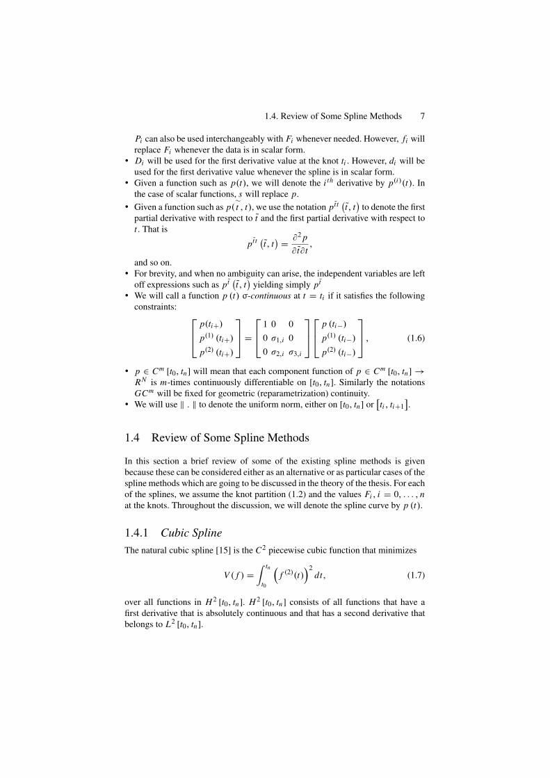
• We will call a function p (t) σ-continuous at t = ti if it satisfies the followingconstraints:
⎡
⎢⎣
p(ti+)
p(1) (ti+)
p(2) (ti+)
⎤
⎥⎦ =
⎡
⎢⎣
1 0 00 σ1,i 00 σ2,i σ3,i
⎤
⎥⎦
⎡
⎢⎣
p (ti−)
p(1) (ti−)
p(2) (ti−)
⎤
⎥⎦ , (1.6)
• p ∈ Cm [t0, tn] will mean that each component function of p ∈ Cm [t0, tn] →RN is m-times continuously differentiable on [t0, tn]. Similarly the notationsGCm will be fixed for geometric (reparametrization) continuity.
• We will use ‖ . ‖ to denote the uniform norm, either on [t0, tn] or[ti , ti+1
].
1.4 Review of Some Spline Methods
In this section a brief review of some of the existing spline methods is givenbecause these can be considered either as an alternative or as particular cases of thespline methods which are going to be discussed in the theory of the thesis. For eachof the splines, we assume the knot partition (1.2) and the values Fi , i = 0, . . . , nat the knots. Throughout the discussion, we will denote the spline curve by p (t).
1.4.1 Cubic SplineThe natural cubic spline [15] is the C2 piecewise cubic function that minimizes
V ( f ) =∫ tn
t0
(f (2)(t)
)2dt, (1.7)
over all functions in H2 [t0, tn]. H2 [t0, tn] consists of all functions that have afirst derivative that is absolutely continuous and that has a second derivative thatbelongs to L2 [t0, tn].
8 1. Introduction
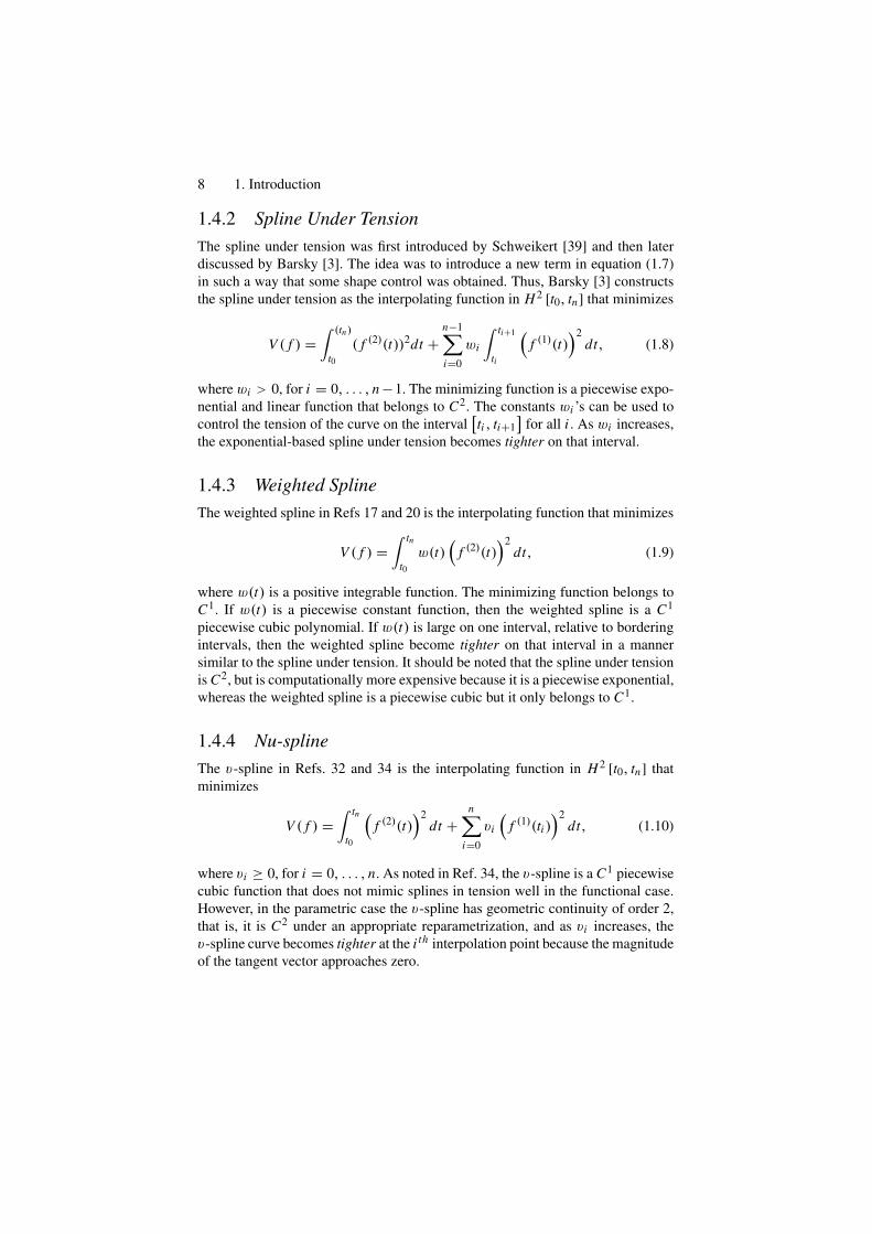
1.4.2 Spline Under TensionThe spline under tension was first introduced by Schweikert [39] and then laterdiscussed by Barsky [3]. The idea was to introduce a new term in equation (1.7)in such a way that some shape control was obtained. Thus, Barsky [3] constructsthe spline under tension as the interpolating function in H2 [t0, tn] that minimizes
V ( f ) =∫ (tn)
t0( f (2)(t))2dt +
n−1∑
i=0
wi
∫ ti+1
ti
(f (1)(t)
)2dt, (1.8)
where wi > 0, for i = 0, . . . , n −1. The minimizing function is a piecewise expo-nential and linear function that belongs to C2. The constants wi ’s can be used tocontrol the tension of the curve on the interval
[ti , ti+1
]for all i . As wi increases,
the exponential-based spline under tension becomes tighter on that interval.
1.4.3 Weighted SplineThe weighted spline in Refs 17 and 20 is the interpolating function that minimizes
V ( f ) =∫ tn
t0w(t)
(f (2)(t)
)2dt, (1.9)
where w(t) is a positive integrable function. The minimizing function belongs toC1. If w(t) is a piecewise constant function, then the weighted spline is a C1
piecewise cubic polynomial. If w(t) is large on one interval, relative to borderingintervals, then the weighted spline become tighter on that interval in a mannersimilar to the spline under tension. It should be noted that the spline under tensionis C2, but is computationally more expensive because it is a piecewise exponential,whereas the weighted spline is a piecewise cubic but it only belongs to C1.
1.4.4 Nu-splineThe v-spline in Refs. 32 and 34 is the interpolating function in H2 [t0, tn] thatminimizes
V ( f ) =∫ tn
t0
(f (2)(t)
)2dt +
n∑
i=0
vi
(f (1)(ti )
)2dt, (1.10)
where vi ≥ 0, for i = 0, . . . , n. As noted in Ref. 34, the v-spline is a C1 piecewisecubic function that does not mimic splines in tension well in the functional case.However, in the parametric case the v-spline has geometric continuity of order 2,that is, it is C2 under an appropriate reparametrization, and as vi increases, thev-spline curve becomes tighter at the i th interpolation point because the magnitudeof the tangent vector approaches zero.
1.4. Review of Some Spline Methods 9
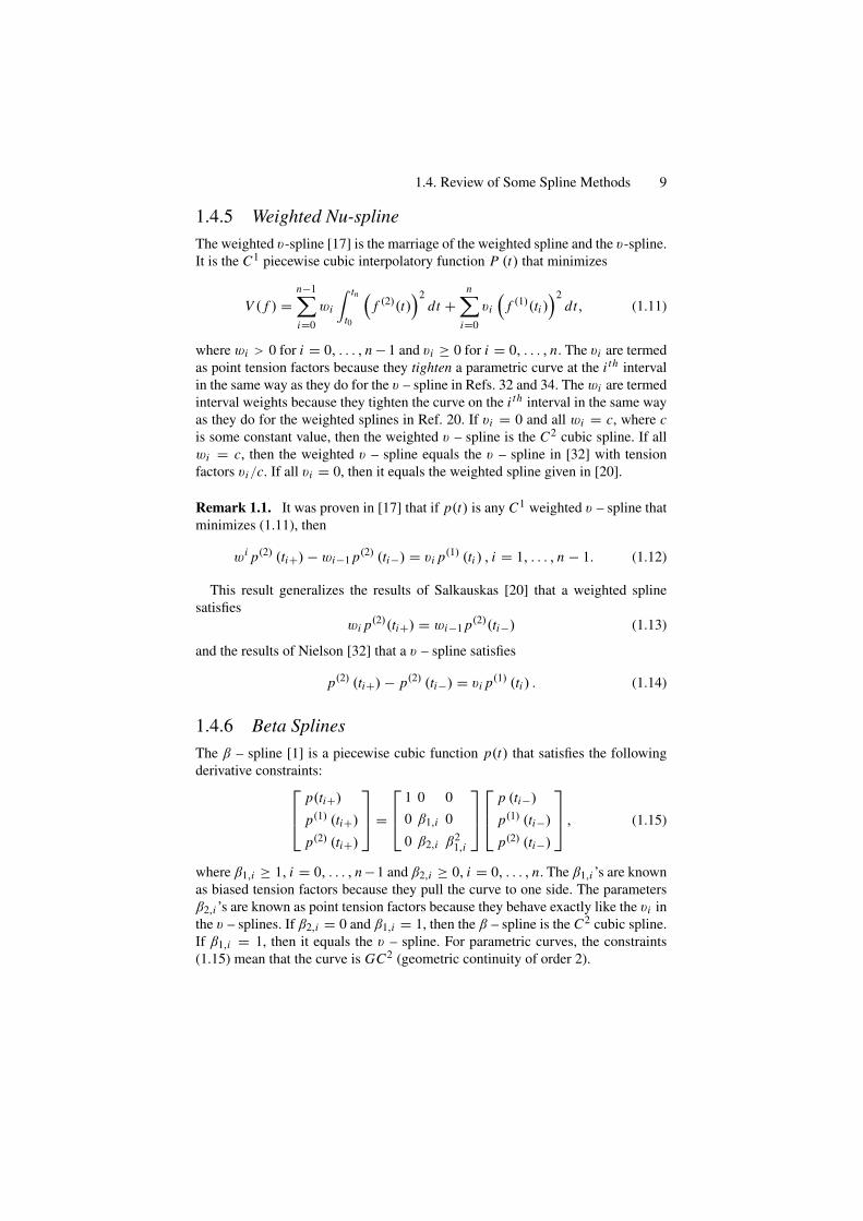
1.4.5 Weighted Nu-splineThe weighted v-spline [17] is the marriage of the weighted spline and the v-spline.It is the C1 piecewise cubic interpolatory function P (t) that minimizes
V ( f ) =n−1∑
i=0
wi
∫ tn
t0
(f (2)(t)
)2dt +
n∑
i=0
vi
(f (1)(ti )
)2dt, (1.11)
where wi > 0 for i = 0, . . . , n − 1 and vi ≥ 0 for i = 0, . . . , n. The vi are termedas point tension factors because they tighten a parametric curve at the i th intervalin the same way as they do for the v – spline in Refs. 32 and 34. The wi are termedinterval weights because they tighten the curve on the i th interval in the same wayas they do for the weighted splines in Ref. 20. If vi = 0 and all wi = c, where cis some constant value, then the weighted v – spline is the C2 cubic spline. If allwi = c, then the weighted v – spline equals the v – spline in [32] with tensionfactors vi/c. If all vi = 0, then it equals the weighted spline given in [20].
Remark 1.1. It was proven in [17] that if p(t) is any C1 weighted v – spline thatminimizes (1.11), then
wi p(2) (ti+) − wi−1 p(2) (ti−) = vi p(1) (ti ) , i = 1, . . . , n − 1. (1.12)
This result generalizes the results of Salkauskas [20] that a weighted splinesatisfies
wi p(2)(ti+) = wi−1 p(2)(ti−) (1.13)
and the results of Nielson [32] that a v – spline satisfies
p(2) (ti+) − p(2) (ti−) = vi p(1) (ti ) . (1.14)
1.4.6 Beta SplinesThe β – spline [1] is a piecewise cubic function p(t) that satisfies the followingderivative constraints:
⎡
⎢⎣
p(ti+)
p(1) (ti+)
p(2) (ti+)
⎤
⎥⎦ =
⎡
⎢⎣
1 0 00 β1,i 0
0 β2,i β21,i
⎤
⎥⎦
⎡
⎢⎣
p (ti−)
p(1) (ti−)
p(2) (ti−)
⎤
⎥⎦ , (1.15)
where β1,i ≥ 1, i = 0, . . . , n−1 and β2,i ≥ 0, i = 0, . . . , n. The β1,i ’s are knownas biased tension factors because they pull the curve to one side. The parametersβ2,i ’s are known as point tension factors because they behave exactly like the vi inthe v – splines. If β2,i = 0 and β1,i = 1, then the β – spline is the C2 cubic spline.If β1,i = 1, then it equals the v – spline. For parametric curves, the constraints(1.15) mean that the curve is GC2 (geometric continuity of order 2).
10 1. Introduction
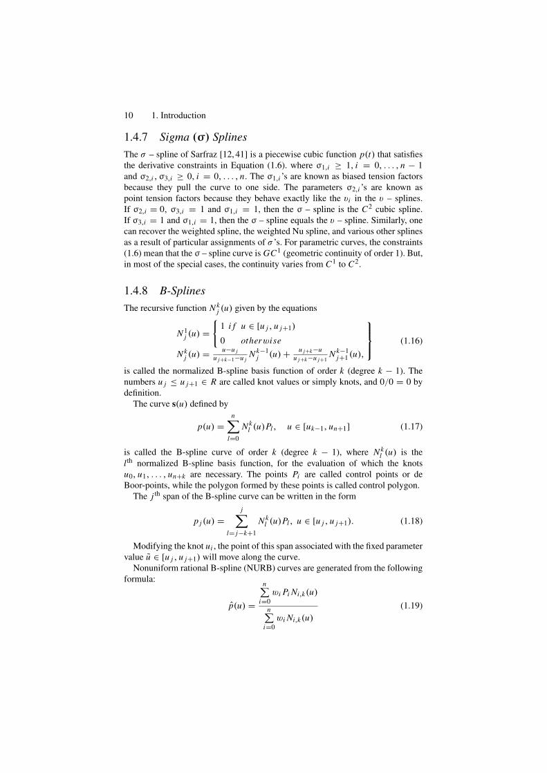
1.4.7 Sigma (σ) SplinesThe σ – spline of Sarfraz [12, 41] is a piecewise cubic function p(t) that satisfiesthe derivative constraints in Equation (1.6). where σ1,i ≥ 1, i = 0, . . . , n − 1and σ2,i ,σ3,i ≥ 0, i = 0, . . . , n. The σ1,i ’s are known as biased tension factorsbecause they pull the curve to one side. The parameters σ2,i ’s are known aspoint tension factors because they behave exactly like the vi in the v – splines.If σ2,i = 0, σ3,i = 1 and σ1,i = 1, then the σ – spline is the C2 cubic spline.If σ3,i = 1 and σ1,i = 1, then the σ – spline equals the v – spline. Similarly, onecan recover the weighted spline, the weighted Nu spline, and various other splinesas a result of particular assignments of σ ’s. For parametric curves, the constraints(1.6) mean that the σ – spline curve is GC1 (geometric continuity of order 1). But,in most of the special cases, the continuity varies from C1 to C2.
1.4.8 B-SplinesThe recursive function N k
j (u) given by the equations
N 1j (u) =
{1 i f u ∈ [u j , u j+1)
0 otherwiseN k
j (u) = u−u ju j+k−1−u j
N k−1j (u) + u j+k−u
u j+k−u j+1N k−1
j+1 (u),
⎫⎪⎬
⎪⎭(1.16)
is called the normalized B-spline basis function of order k (degree k − 1). Thenumbers u j ≤ u j+1 ∈ R are called knot values or simply knots, and 0/0 = 0 bydefinition.
The curve s(u) defined by
p(u) =n∑
l=0
N kl (u)Pl , u ∈ [uk−1, un+1] (1.17)
is called the B-spline curve of order k (degree k − 1), where N kl (u) is the
l th normalized B-spline basis function, for the evaluation of which the knotsu0, u1, . . . , un+k are necessary. The points Pi are called control points or deBoor-points, while the polygon formed by these points is called control polygon.
The j th span of the B-spline curve can be written in the form
p j (u) =j∑
l= j−k+1
N kl (u)Pl , u ∈ [u j , u j+1). (1.18)
Modifying the knot ui , the point of this span associated with the fixed parametervalue u ∈ [u j , u j+1) will move along the curve.
Nonuniform rational B-spline (NURB) curves are generated from the followingformula:
p(u) =
n∑
i=0wi Pi Ni,k(u)
n∑
i=0wi Ni,k(u)
(1.19)
1.4. Review of Some Spline Methods 11
where Pi , i = 0, 1, . . ., n, are control points, wi are weights, and Ni,k(u) areB-spline basis functions.
1.4.9 Bezier SplinesGiven (n + 1) points Pi : i = 0, 1, 2, . . ., n, Bezier curve is defined as follows:
P(t) =n∑
i=0
Pi Bi (t), 0 ≤ t ≤ 1, (1.20)
whereBi (t) =
(ni
)(1 − t)n−i t i ,
are Bernstein polynomials. Here we will refer to Bi (t)’s as Bezier blending func-tions. For example, for n = 3, equation (1.20) will reduce to:
P(t) =n∑
i=0
Pi Bi (t),
= P0 B0(t) + P1 B1(t) + P2 B2(t) + P3 B3(t),
=(
30
)(1 − t)3 P0 + P1
(31
)(1 − t)2t + P2
(32
)(1 − t)t2 + P3t3,
= (1 − t)3 P0 + 3P1(1 − t)2t + 3P2(1 − t)t2 + P3t3. (1.21)
The polynomials
(1 − t)3, 3(1 − t)2t, 3(1 − t)t2, t3,
are called Bezier cubic blending functions. The convex hull of points Pi , i =0, 1, . . ., n is (roughly speaking) the region surrounded by Pi ’s. The points Pi ’sare also known as control points, and the polygon connected by Pi ’s is calledcontrol polygon. There are some interesting properties worth noting:
1. The degree of a Bezier curve is one less than the given control points.2. The Bezier curve always pass through the first and last points.3. The Bezier curve always remains within the convex hull of the control polygon.4. The Bezier curve always satisfies the variation diminishing property. That is,
the property that curve does not cross any straight line more than the controlpolygon crosses.
1.4.10 Hermite SplinesLet
P (0) = P0, P (1) = P3, P(1) (0) = D0, P(1) (1) = D1.
12 1. Introduction
Then (1.21) becomes like the following:
P(t) = (1 − t)3 P0 + 3t (1 − t)2(
P0 + D0
3
)+ 3t2(1 − t)
(P3 − D1
3
)+ t3 P3.
(1.22)
The curve in equation (1.22) is called Hermite cubic curve where 0 ≤ t ≤ 1 canbe interchanged with 0 ≤ θ ≤ 1 without loss of generality. Higher-degree Hermitecurves can also be defined in a similar manner. To have a more precise and generalnotation for a Hermite cubic spline curve, let us adopt the following:
P (0) = Pi , P (1) = Pi+1, P(1) (0) = Di , P(1) (1) = Di+1.
Then, the Hermite curve takes the following form:
P(t) = (1 − θ)3 Pi + 3θ(1 − θ)2(
Pi + hi Di
3
)
+3θ2(1 − θ)
(Pi+1 − hi Di+1
3
)+ θ3 Pi+1, (1.23)
where θ and hi are defined in equations (1.3) and (1.4). If we have the points asfollows:
P0, P1, P2, . . ., Pn (1.24)
Then, we can fit Hermite curve pieces between each pair of points for i =0, 1, 2, . . . , n − 1. The curve represented in (1.24) is called a Hermite spline pro-vided the information about the tangents Di ’s is given. Let us define Di ’s as fol-lows:
D0 = 2(P1 − P0) − (P2 − P0)/2,Dn = 2(Pn − Pn−1) − (Pn − Pn−2)/2,Di = ai (Pi − Pi−1) + (1 − ai )(Pi+1 − Pi ), i = 1, 2, 3, . . . , n − 1,
⎫⎬
⎭(1.25)
whereai = |Pi+1 − Pi |
|Pi+1 − Pi | + |Pi − Pi−1| .Although the tangents provided in equations (1.25) will produce open curves,
they can be easily oriented to produce closed curves too.The Hermite spline P(t) will be called a cardinal spline provided the derivative
values Di ’s are changed as follows:
Di = 12(1 − αi )(Pi+1 − Pi−1),
Di+1 = 12(1 − αi )(Pi+2 − Pi ).
In this case, we would have the curve segments for i = 1, 2, . . . , n − 2. Theparameter αi is called tension parameter because it tightens or loosens the curvewhen it increases or decreases. When αi = 0, the cardinal spline is called Catmull-Rom spline or Overhauser spline.

References 13
The Hermite spline P(t) will be called a Kochanek-Bartels spline provided thederivative values Di ’s are changed as follows:
Di = 12(1 − αi )
[(1 + βi )(1 − γi )(Pi − Pi−1) + (1 − βi )(1 + γi )(Pi+1 − Pi )
],
Di+1 = 12(1 − αi )
[(1 + βi )(1 − γi )(Pi+1 − Pi ) + (1 − βi )(1 + γi )(Pi+2 − Pi+1)
],
where
• αi is a tension parameter.• βi is a biased parameter.• γi is a continuity parameter.
The parameter values βi = 0 = γi produce the cardinal spline.
1.5 Summary
This chapter provides introductory material that is useful before studying the restof the book. It provides notation, a summary of spline methods and their history,and a rich bibliography. The chapter also describes who should study the book.Some valuable suggestions have also been made regarding the structure of thebook for course work at both the undergraduate and graduate levels.
1.6 Exercises
1. What is this book about?2. What is a spline?3. Name at least 10 spline methods in the literature.4. Write programs to plot the following spline curves:
(a) Quadratic B-spline(b) Cubic B-spline(c) Bezier curves of arbitrary degree.(d) Cubic Hermite spline(e) Cardinal spline(f) Kochanek Bartel spline.
5. Name at least 20 applications where a spline can be used.
References1. Barsky, B.A. (1981), The Beta-spline: a local representation based on shape parame-
ters and fundamental-geometric measure, Ph.D. thesis, University of Utah.2. Barsky, B.A., and Beatty, J.C. (1983), Local control of bias and tension in beta-
splines, ACM Trans Graphics 2, 109–134.

14 1. Introduction
3. Barsky, B.A. (1984), Exponential and polynomial methods for applying tension to aninterpolating spline curve, Comput Vision Graph lmage Process 27, 1–18.
4. Bartels, R., and Beatty, J. (1984), Beta-splines with a difference. Technical report CS-83-40, Waterloo Computer Science Department, Waterloo, Ontario, Canada N2L3Gl.
5. Boehm, W., Farin, G., and Kahmann, J. (1984), A survey of curve and surface methodsin CAGD, Comput Aided Geom Des 1(1), 1–60.
6. Boehm, W. (1985), Curvature continuous curves and surfaces, Comput Aided GeomDes 2(2), 313–323.
7. Boehm, W. (1986), Smooth curves and surfaces, in Farin, G.E., ed. Geometric Mode-ling, pp. 175–184.
8. Boehm, W. (1987), Rational geometric splines, Comput Aided Geom Des 4, 67–77.9. Cline, A. (1974), Curve fitting in one and two dimensions using splines under tension,
Comm ACM 17, 218–223.10. De Boor, C. (1978), A Practical Guide to Splines. Springer-Verlag, New York.11. Delbourgo, R., and Gregory, J.A. (1985), Shape-preserving piecewise rational inter-
polation, SIAM J Stat Comput 6, 967–976.12. Sarfraz, M. (1994), Generalized geometric interpolation for rational cubic splines, Int
J Comput Graphics, Elsevier Science, 18(1), 61–72.13. Dierckx, P., and Tytgat, B. (1989), Generating the Bezier points of a β-spline curve,
Comput Aided Geom Des 6, 279–291.14. Farin, G.E. (1983), Algorithms for rational Bezier curves, Comput Aided Des 15,
73–77.15. Farin, G.E. (1988), Curves and Surfaces for Computer-Aided Geometric Design,
Academic Press, New York.16. Foley, T.A. (1986), Local control of interval tension using weighted splines, Comput
Aided Geom Des 3, 281–294.17. Foley, T.A. (1987), Interpolation with interval and point tension controls using cubic
weighted v-splines, ACM Trans Math Soft 13, 68–96.18. Foley, T.A., and Ely, H.S. (1989), Surface interpolation with tension controls using
cardinal bases, Comput Aided Geom Des 6, 97–109.19. Fritsch, F.N., and Carlson, R.E. (1980), Monotone piecewise cubic interpolation,
SIAM J Numer Anal 17(2), 238–246.20. Salkauskas, K. (1984), C1 splines for interpolation of rapidly varying data, Rocky Mtn
J Math 14, 239–250.21. Goldman, R.N., and Barsky, B.A. (1989), On beta-continuous functions and their
application to the construction of geometrically continuous curves and surfaces, inLyche, T., and Schumaker, L., eds. Mathematical Methods in Computer-Aided Geo-metric Design, Academic Press, New York.
22. Goodman, T.N.T., and Unsworth, K. (1985), Generation of beta-spline curves usinga recursive relation, in R.E. Earnshaw, ed., Fundamental Algorithms for ComputerGraphics, Springer-Verlag, Berlin, pp. 326–357.
23. Goodman, T.N.T. (1988), Shape-preserving interpolation by parametric rational cubicsplines, Proc Int Conf on Numerical Mathematics, Int Ser Num Math 86, Birkhauser-Verlag, Basel.
24. Goodman, T.N.T., and Unsworth, K. (1988), Shape-preserving interpolation by para-metrically defined curves, SIAM J Numer Anal 25, 1–13.
25. Goodman, T.N.T. (1989), Shape-preserving representations, in Lyche, T., andSchumaker, L., eds., Mathematical Methods in Computer-Aided Geometric Design,Academic Press, New York.

References 15
26. Gordon, W.J. (1971), Blending function methods of bivariate and multivariate inter-polation and approximation, SIAM J Num Anal 8, 158–177.
27. Gregory, J.A. (1986), Shape-preserving spline interpolation, Comput Aided Des 18,53–57.
28. Gregory, J.A., and Sarfraz, M. (1990), A rational spline with tension, Comput AidedGeom Des 7, 1–13.
29. Hohmeyer, M.E., and Barsky, B.A. (1989), Rational continuity, to appear in TransComputer Graphics.
30. Kochanek, D.H., and Bartels R.H. (1984), Interpolating splines with local tension:Continuity and biased control, Comput Graphics 18, 33–41.
31. Lewis, J. (1975), “B-spline” bases for splines under tension, nu-splines, and fractionalorder splines. Presented at the SIAM-SIGNUM Meeting, San Francisco, CA.
32. Nielson, G.M. (1974), Some piecewise polynomial alternatives to splines under ten-sion, in Barnhill, R.F., eds., Computer-Aided Geometric Design, Academic Press,New York.
33. Nielson, G.M. (1984), A locally controllable spline with tension for interactive curvedesign, Comput Aided Geom Des 1, 199–205.
34. Nielson, G.M. (1986), Rectangular υ-splines. IEEE Comput Graphics Appl 6, 35–40.35. Preuss, S. (1976), Properties of splines in tension, J Approx Theory 17, 86–96.36. Preuss, S. (1979), Alternatives to the exponential spline in tension, Math. Comp. 33,
1273–128137. Sarfraz M. (1987), Spline curve interpolation with shape control M.Sc. dissertation,
Brunel University, U.K.38. Schoenberg, L. (1981), Spline Functions: Basic Theory, John Wiley, New York.39. Schweikert, D. (1966), An interpolation curve using splines in tension, J Math Phys
45, 312–317.40. Spath, H . (1974), Spline Algorithms for Curves and Surfaces, Utilitas Mathematica,
Winnipeg.41. Sarfraz, M. (1990), The representation of curves and surfaces in computer-aided geo-
metric design using rational cubic splines, Ph.D. thesis, Brunel University, UK.42. Sarfraz, M. (1992), A C2 rational cubic spline alternative to the NURBS, Comp &
Graph 16(l), 69–78.43. Sarfraz, M. (1995), Curves and surfaces for CAD using C2 rational cubic splines,
Int J Eng Comput, Springer-Verlag, 11(2), 94–102.44. Sarfraz, M. (1994), Freeform rational bicubic spline surfaces with tension control,
Facta Universitatis (Nis), Series Mathematics and Informatics, Vol. 9, 83–93.45. Sarfraz, M. (1994), Cubic spline curves with shape control, Int J Comput Graphics,
Elsevier Science, 18(5), 707–713.46. Sarfraz, M, (2003), Weighted nu-splines: an alternative to NURBS, in Advances in
Geometric Modeling, M. Sarfraz, ed., John Wiley, New York, pp. 81–95.47. Schoenburg, I.J. (1946), Contributions to the problem of approximation of equidistant
data by analytic functions, Appl Math 4, 45–99.48. Schweikert, D.G. (1966), An Interpolation curve using a spline in tension, J Math
Phys 45, 312–317.49. Sarfraz, M. (2004), Weighted nu-splines with local support basis functions, Int J Com-
put Graphics, Elsevier Science, 28(4), 539–549.50. Sarfraz, M., Butt, S., and Hussain, M.Z. (2001), Visualization of shaped data by a
rational cubic spline interpolation, Int J Comput Graphics, Elsevier Science, 25(5),833–845.

16 1. Introduction
51. Sarfraz, M. (2000), A rational cubic spline for the visualization of monotonic data,Comput Graphics, 24(4), 509–516.
52. Sarfraz, M., and Hussain, M.Z. (2006), Data visualization using rational spline inter-polation, Int J Computat Appl Math, Elsevier Science, 189(1–2), 513–525.
53. Sarfraz, M., Hussain, M.Z., and Chaudhry, F.S. (2005), Shape-preserving cubic splinefor data visualization, Int J Comput Graphics & CAD/CAM, International Scientific,1(6), 185–194.
54. Sarfraz, M. (2002), Visualization of positive and convex data by a rational cubicspline, Int J Infor Sci, Elsevier Science, 146(1–4), 239–254.
55. Sarfraz, M. (2002), Modelling for the visualization of monotone data, Int J ModellingSimulation, ACTA Press, 22(3), 176–185.
56. Holzle, G.E. (1983), Knot placement for piecewise polynomial approximationof curves. Comput Aided Des 15(5), 295–296.
57. Juhasz, I., and Hoffmann, M. (2001) The effect of knot modifications on the shapeof beta-spline curves. J Geom Graphics 5(2), 111–119.
58. Pratt, M., Goult, R., and He, L. (1993), On rational parametric curve approximation.Comput Aided Geom Des 10(3/4):363–377.
59. Razdan, A. (1999), A Knot Placement for B-Spline Curve Approximation. PRISMPublications.
60. Sarfraz, M., Asim, M.R. and Masood, A. (2004), Capturing outlines using cubicBezier curves. Proceedings of 1st IEEE International Conference on Information &Communication Technologies: From Theory to Applications, 2004.
61. Speer, T., Kuppe, M., and Hoschek., J. (1998), Global reparametrization for curveapproximation. Comput Aided Geom Des 15, 869–877.
62. Masood, A., Sarfraz, M., and Haq, S.A. (2005), Curve approximation with quadraticB-splines, Proceedings of IEEE International Conference on Information Visualisa-tion (IV’2005)-UK, IEEE Computer Society Press, 991–996.
63. Sarfraz, M., and Raza, A. (2002), Visualization of data using genetic algorithm, SoftComputing and Industry: Recent Applications, Eds.: R. Roy, M. Koppen, S. Ovaska,T. Furuhashi, and F. Hoffmann, Springer-Verlag, New York, pp. 535–544.
64. Sarfraz, M., and Raza, A., (2002), Visualization of data with spline fitting: a tool witha genetic approach, The Proc. International Conference on Imaging Science, Systems,and Technology (CISST 2002), Las Vegas, Nevada, CSREA Press, pp. 99–105.
65. Taponecco, F., and Alexa, M. (2003), Piecewise circular approximation of spirals andpolar polynomials, Proc. of WSCG 2002, Plzen, Czech. Republic.
66. Taponecco, F., and Alexa, M. (2002), Scan converting spirals, Proc. of WSCG 2002,Plzen, Czech. Republic.
67. Rieger, T., and Taponecco, F. (2002), Interactive Information visualization of entity-relationship data, Proc. of WSCG 2002, Plzen, Czech. Republic
68. Van Aken, J.R., and Novak, M. (1985), Curve drawing algorithms for raster displays,ACM Trans. on Graphics, 4, 147–169.
69. Cook, A.S. (1979), The Curves of Life: Being an Account of Spiral Formations andTheir Application to Growth in Nature, to Science and to Art: with Special Referenceto the Manuscripts of Leonardo Da Vinci, Dover, New York.
70. Habib, Z., and Sakai, M. (2002), T-cubic and arc/T-cubic spirals for web-basedvisualization of planar data. The Proceedings of the Fourth IEEE Workshop onInformation and Computer Science: Internet Computing (WICS’2002), KFUPM,Saudi Arabia, IEEE Computer Society Chapter, pp. 267–278.
References 17
71. Habib, Z., and Sakai, M. (2005), Conic spiral spline, International Conference onGeometric Modeling, Visualization & Graphics, JCIS, pp. 1653–1656.
72. Habib, Z., and Sakai, M. (2005), Web-based Visualization of Conic and Arc/ConicSpirals, International Journal of Computer Graphics & CAD / CAM, 1(1), 16–26.
73. Beus, H.L., and Tiu, S.S.H. (1987), An improved corner detection algorithm based onchain coded plane curves, Pattern Recognition, 20:291–296.
74. Chetverikov, D., and Szabo, Z. (1999), A simple and efficient algorithm for detec-tion of high curvature points in planner curves, Proc. of 23rd Workshop of AustralianPattern Recognition Group, Steyr, pp. 175–184.
75. Davies, E.R. (1988), Application of generalized Hough transform to corner detection,IEE-P(E:135), No. 1, pp. 49–54.
76. Freeman, H., and Davis, L.S. (1977), A corner finding algorithm for chain-codedcurves, IEEE Trans. Computers, 26:297–303.
77. Liu, H.C., and Srinath, L.S. (1990), Corner detection from chain-code, Pattern Recog-nition, 23:51–68.
78. Rattarangsi, A., and Chin, R.T. (1992), Scale-based detection of corners of planarcurves, Trans. Pattern Analysis and Machine Intelligence, 14:430–449.
79. Rosenfeld, A., and Weszka, J.S. (1975), An improved method of angle detection ondigital curves, IEEE Trans. Computer, 24:940–941.
80. Rutkowski, W.S., and Rosenfeld, A. (1978), A comparison of corner-detection tech-niques for chain-coded curves, TR-623, Computer Science Center, University ofMaryland.
81. Sarfraz, M., Asim, M.R., and Masood, A. (2006), A New Approach to Corner Detec-tion: Computer Vision and Graphics, Eds.: Konrad Wojciechowski, Bogdan Smolka,Henryk Palus, Ryszard S. Kozera, Wladyslaw Skarbek, Lyle Noakes, Springer-Verlag,New York, pp. 528–533.
82. The, C. and Chin, R. (1990), On the detection of dominant points on digital curves,IEEE Trans. PAMI 8:859–873.
83. Wang, H., and Brady, M. (1995), Real-time corner detection algorithm for motionestimation, Image and Vision Computing, 13(9), 695–703.
84. Masood, A., and Sarfraz, M. (2006), A novel corner detector approach using slid-ing rectangles, The Proceedings of The 4th ACS/IEEE International Conference onComputer Systems and Applications (AICCSA-06), Sharja, UAE, pp. 621–626, IEEEComputer Society Press.
85. Karow P. Digital Typefaces: Description and Formats. Springer-Verlag, Berlin, 1994.86. Karow P. Font Technology Methods and Tools. Springer-Verlag, Berlin, 1994.87. Cox, M.G. (1971), Curve fitting with piecewise polynomials. J. Inst. Math Applica-
tions 8, 36–52.88. Plass, M., and Stone, M. (1983), Curve fitting with piecewise parametric cubics. Com-
puter Graphics, 17(3), 229–239.89. Zhang, S., Li, L., Seah, H.S. (1998), Recursive curve fitting and rendering. The Visual
Computer, 69–82, 1998.90. Sarfraz, M. and Khan, M.A. (2004), An automatic algorithm for approximating
boundary of bitmap characters, Future Generation Computer Systems, Elsevier Sci-ence, Vol. 20, 1327–1336.
91. Sarfraz, M. (2004), Some algorithms for curve design and automatic outline capturingof images, International Journal of Image and Graphics, World Scientific Publisher,4(2), 301–324.
18 1. Introduction
92. Sarfraz, M. (2003), Curve fitting for large data using rational cubic splines, Interna-tional Journal of Computers and Their Applications, 10(4), 233–246.
93. Sarfraz, M., and Khan, M.A. (2003), An automatic outline fitting algorithm for Arabiccharacters, Lecture Notes in Computer Science, Vol. 2669: Computational Scienceand Its Applications, Eds.: V. Kumar, M.L. Gavrilova, C.J.K. Tan, and P. L’Ecuyer,Springer-Verlag, New York, pp. 589–598.
94. Sarfraz, M. (2003), Optimal curve fitting to digital data, International Journal ofWSCG, 11(1), 128–135.
95. Sarfraz, M., and Razzak, M.F.A., (2003), A web-based system to capture outlines ofArabic fonts, International Journal of Information Sciences, Elsevier Science Inc.,150(3–4), 177–193.
96. Sarfraz, M., and Razzak, M.F.A., (2002), An algorithm for automatic capturing of fontoutlines, International Journal of Computers & Graphics, Elsevier Science, 26(5),795–804.
97. Sarfraz, M., and Khan, M.A. (2002), Automatic outline capture of Arabic fonts, Inter-national Journal of Information Sciences, Elsevier Science, 140(3–4), 269–281.
98. Sarfraz, M., Riyazuddin, M., and Baig, M.H. (2006), Capturing planar shapes byapproximating their outlines, International Journal of Computational and AppliedMathematics, Elsevier Science, 189(1–2), 494–512.
99. Sarfraz, M. (2004), Representing shapes by fitting data using an evolutionaryapproach, International Journal of Computer-Aided Design & Applications, 1(1–4),179–186.
100. Sarfraz, M, and Raza, A. (2002), towards automatic recognition of fonts using agenetic approach, Recent Advances in Computers, Computing, and Communications,Eds.: N. Mastorakis and V. Mladenov, WSEAS Press, 290–295.
101. Sarfraz, M. (2003), Outline representation of fonts using a genetic approach,Advances in Soft Computing: Engineering Design and Manufacturing, Eds.: Benitez,J.M., Cordon, O., Hoffmann, F., and Roy, R., Springer-Verlag, 109–118.
102. Sarfraz, M., Asim, M.R., and Masood, A. (2004), Piecewise polygonal approximationof digital curves, The Proceedings of IEEE International Conference on InformationVisualisation (IV’2004)-UK, IEEE Computer Society Press, 991–996.
103. Dierckx, P. (1993), Curve and Surface Fitting with Splines. Clarendon Press (1993).104. Farin, G. (1989), Trends in curves and surface design. Computer-Aided Design, 21(5),
293–296.105. Piegl, L., and Tiller, W. (1991), Curve and surface reconstruction using rational B-
splines. Computer-Aided Design, 19(9), 485–498.106. Cho, M-W, Seo, T-I, Kim, J-D, and Kwon, O-Y, (2000), Reverse engineering of
compound surfaces using boundary detection method, Korean Society of Mechani-cal Engineers International Journal, 14(10), 1104–1113.
107. Laurent-Gengoux, P., and Mekhilef, M. (1993), Optimization of a NURBS represen-tation, Computer-Aided Design, 25(11), 699–710.
108. Sarfraz, M. (2006), Computer-aided reverse engineering using simulated evolution onNURBS, International Journal of Virtual & Physical Prototyping, Taylor & Francis,New York, 1(4), 494–512.
109. Gershon, E., and Gotsman, C. (1995), Multiresolution control for nonuniformB-spline curve editing, in Pacific Graphics ’95.
110. Finkelstein, A., and Salesin, D.H. (1994), Multiresolution curves, in Proceedings ofSIGGRAPH, pp. 261–268, ACM, New York.

References 19
111. Grisoni, L., Schlick C., and Blanc, C. (1997), An Hermitian Approach for Multireso-lution Splines, Technical Report No. 1192–97, LaBRI.
112. Stollnitz Eric J., DeRose Tony D., and Salesin David H. (1995), Wavelets for com-puter graphics: a primer, part-1, IEEE Computer Graphics and Applications, 15(3),76–84.
113. Stollnitz E.J., DeRose T.D., and Salesin D.H. (1995), Wavelets for computer graphics:a primer, part-2, IEEE Computer Graphics and Applications, 15(4), 75–85.
114. Stollnitz E.J., DeRose T.D., and Salesin D.H. (1996), Wavelets for Computer Graph-ics: Theory and Applications, Morgan Kaufman Publishers, San Francisco.
115. Sarfraz, M., and Siddiqui, M.A. (2004), Development of a multi-resolution frame-work for NUBS, International Journal of Information Sciences, Elsevier Science,163(4), 239–251.
2Weighted Nu Splines
Abstract. Weighted ν-splines are the composition of two spline methods, namely, weightedsplines and ν-splines. These are the generalization of cubic spline method and arehighly useful for CAD/CAM and various applications in computer graphics. Both—interpolatory and freeform—schemes are available in the literature. This chapter explainsinterpolatory weighted ν-splines together with a construction of its B-spline-like form.The design curves, constructed through B-spline-like form, possess all the ideal geometricproperties such as partition of unity, convex hull, and variation diminishing. The splinesprovide not only a variety of very interesting shape control such as point and intervaltensions but also, as a special case, recover the cubic spline method. In addition, theseweighted ν-splines also provide, as special cases, the weighted splines and the ν-splines.The method for evaluating these splines is suggested by a transformation to Bezier form.
2.1 Introduction
Designing of curves, especially those curves that are robust and easy to control andcompute, has been one of the significant problems of computer graphics and geo-metric modeling. Specific applications including font designing, capturing hand-drawn images on computer screens, data visualization, and computer-supportedcartooning are main motivations toward curve designing. In addition, various otherapplications in CAD/CAM/CAGD are also a good reason to study this topic. Manyauthors have worked in this direction. For brevity, the reader is referred to [1–22].
A cubic spline curve method is considered to be a considerably decent approachfor designing applications in the area of computer graphics and geometric mod-eling. However, due to its various limitations, such as lack of freedom in shapecontrol, a designer may not have much help. In this study, the weighted ν-splinemethod has been reviewed. This curve design method, in addition to enjoying thegood features of cubic splines, possesses interesting shape design features too.It has two families of shape parameters working in such a way that one familyof parameters is associated with intervals and the other with points. These para-meters provide a variety of shape control such as point and interval tension. Thisis an interpolatory curve scheme, which utilizes a piecewise cubic function in itsdescription. However, it is desired to extend this idea to freeform curves, which
21
22 2. Weighted Nu Splines
can enjoy all the ideal properties related to B-spline theory. This work is mainlyconcerned with developing such a theory.
Weighted splines [7] were discovered as a cubic spline method. The methodprovides a C1 computationally simpler alternative to the exponential spline-under-tension [4, 13, 20]. Regarding shape characteristics, it has shape control parame-ters associated with each interval, which can be used to flatten or tighten the curvelocally. Nu-splines [11,12] were discovered as another cubic spline method. It pro-vides a GC2 computationally simpler alternative to the exponential spline-under-tension [4,13,21]. Regarding shape characteristics, it has shape control parametersassociated with each point, which can be used to tighten the curve both locally andglobally. The ideas of weighted splines and Nu-splines were married together toformulate another spline called weighted Nu-spline [11, 12, 19, 22]. This curvedesign method covers the shape features of both of its counter parts and providesa C1 computationally economical method.
B-splines are a useful and powerful tool for computer graphics and geometricmodeling. They can be found frequently in the existing CAD/CAM (computer-aided design/computer -aided manufacturing) systems. They form a basis for thespace of n th degree splines of continuity class Cn−1. Each B-spline is a non-negative n th-degree spline that is nonzero only on n + 1 intervals. The B-splinesform a partition of unity, that is, they sum up to one. Curves generated by summingcontrol points multiplied by the B-splines have some very desirable shape proper-ties, including the local convex hull property and variation diminishing property.
It is desirable to generalize the idea of B-spline-like local basis functions for theclasses of splines with shape parameters considered in the description of continu-ity. The first local basis for GC2 splines was developed by Lewis [10]. In 1981,Barsky [1] generalized B-splines to Beta splines. These splines preserve the geo-metric smoothness of the design curve while allowing the continuity conditionson the spline functions at the knots to be varied by certain parameters, thus givinggreater flexibility. Later, in 1984, Bartels and Beatty [2] developed local bases forBeta spline curves that are equivalent to Boehm’s [3] Gamma splines. Foley [7],in 1987, constructed a B-spline-like basis for weighted splines; different weightswere built into the basis functions so that the control point curve was a C1 piece-wise cubic with local control of interval tension.
In this work, a constructive approach has been adopted to build B-spline-likebasis for cubic spline curves with the same continuity constraints as those for inter-polatory weighted v-splines. These are local basis functions with local supportwhich have the property of being positive everywhere. The design curve, con-structed through these functions, possesses all the ideal geometric properties likepartition of unity, convex hull, and variation diminishing. This curve method pro-vides not only a variety of very interesting shape control such as point and intervaltensions, but also, as a special case, recovers the cubic B-spline curve method.In addition, it also provides B-spline-like design curves for weighted splines,ν-splines and weighted ν-splines. The method for evaluating these splines issuggested by a transformation to Bezier form.
2.2. Some Spline Methods 23
The approach adopted in the construction of local basis for the weightedν-splines is quite different from those adopted for different spline methodsin [1–8, 15]. The way for evaluating the weighted ν-splines representation ofa curve is suggested by a transformation to piecewise defined Bezier form. Thisform will also expedite a proof of the variation diminishing property for the Bezierrepresentation.
This chapter is related the weighted ν-spline method [19, 22] explained inSection 2.2. It studies, in Section 2.3, a B-spline-like local basis for the weightedν-spline. The design curve in Section 2.4 maintains the C1 continuity of theweighted ν-splines. This description of freeform weighted ν-spline not only pro-vides a variety of interesting shape control such as point and interval tensionsbut also, as a special case, recovers the cubic B-spline curve method. In addition,it also provides B-spline like design curves for weighted splines, ν-splines andweighted ν-splines. The method has been extended for the construction of surfacesin Section 2.5. Section 2.6 summarizes the chapter.
2.2 Some Spline Methods
This section gives a brief review of the cubic spline, weighted splines, ν-splines,and weighted ν-splines. Detailed description of the weighted ν-splines is given inSections 2.3 and 2.4. Assume that we are given knot partition as t1 < t2 < . . . . <tn , and set of control points F1, F2, . . . , Fn . Let us have the Followings:
Point tension factors: νi ≥ 0, i = 1, 2, . . . , n,
Interval weights: wi > 0, i = 1, 2, . . . , n.
}
, (2.1)
Consider the piecewise cubic function:
p(t) ≡ pi (t) = Fi (1 − θ)3 + 3θ(1 − θ)2Vi + 3θ2(1 − θ)Wi + Fi+1θ3, (2.2)
whereθ = t − ti
hi, hi = ti+1 − ti , (2.3)
andVi = Fi + hi Di
3, Wi = Fi+1 − hi Di+1
3. (2.4)
It is obvious to see that the piecewise cubic function (2.2) holds the followinginterpolatory properties:
p(ti ) = Fi , p(ti+1) = Fi+1
p(1)(ti ) = Di , p(1)(ti+1) = Di+1
}
, (2.5)
where p(1) denotes first derivative with respect to t and Di denote derivative valuesgiven at the knots ti . This leads the piecewise cubic (2.2) to the piecewise Hermiteinterpolant p ∈ C1[t1, tn].
24 2. Weighted Nu Splines
2.2.1 Cubic SplinesThe cubic spline interpolant is a C2 piecewise cubic function p(t) that minimizes
V ( f ) =n−1∑
i=1
ti+1∫
ti
[f ′′(t)
]2dt,
subject to the interpolation conditions f (ti ) = Fi for i = 1, 2, . . . , n and one ofthe following end conditions:
• Type 1: First derivative end conditions,• Type 2: Natural end conditions, or• Type 3: Periodic end conditions.
Given Fi and Di for i = 1, 2, . . . , n, there exists a unique C2 piecewise cubicfunction f (t) that satisfies f (ti ) = Fi and f ′(ti ) = Di for i = 1, 2, . . . , n.The unknowns are the first derivative values, Di , i = 1, 2, . . . , n, and once theyare computed, the function f (t) can be easily evaluated using the standard piece-wise cubic Hermite form explained in (2.2). Necessary and sufficient conditionsfor the function f (t) to be the cubic spline interpolant are that its derivatives Di ’ssatisfy
ci−1 Di−1 + (2ci−1 + 2ci)
Di + ci Di+1 = bi (Fi+1 − Fi ) + bi−1 (Fi − Fi−1) ,
for i = 1, 2, . . . , n, where ci = 1/hi , bi = 3ci/hi . The above system of equa-tions provides (2.n −2) equations for n unknowns, D1, . . ., Dn , and the additionalequations come from the given end conditions. The equations for Type I first deriv-ative end conditions are D1 = f ′(t1) and Dn = f ′(tn). For Type II natural endconditions they are
2c1 D1 + c1 D2 = b1 (F2 − F1) ,
andcn−1 Dn−1 + 2cn−1 Dn = bn−1(Fn − Fn−1).
For Type 3 periodic end conditions, they are(2c1 + 2cn−1
)D1 + c1 D2 + cn−1 Dn−1 = b1(F2 − F1) + bn−1(Fn − Fn−1),
and D1 = Dn . The linear system of equations that occurs when Type 1 or 2end conditions are used is tridiagonal and diagonally dominant; thus it can besolved efficiently by using a standard tridiagonal system solver. Figure 2.1 is acubic spline curve for a data shown as bullets.
2.2.2 Weighted SplinesThe weighted spline interpolant is a C1 piecewise cubic function p(t) that mini-mizes
V ( f ) =n−1∑
i=1
ωi
ti+1∫
ti
[f ′′(t)
]2dt,
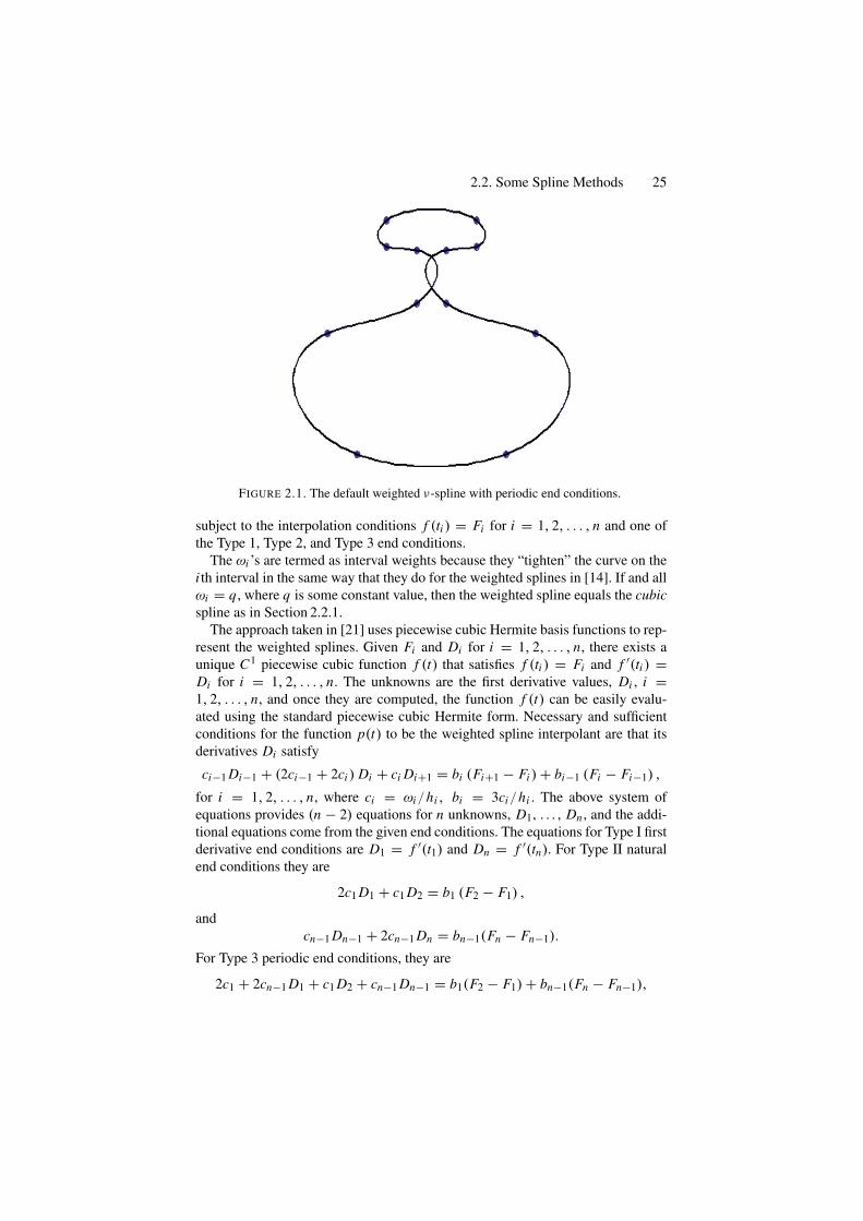
2.2. Some Spline Methods 25
FIGURE 2.1. The default weighted ν-spline with periodic end conditions.
subject to the interpolation conditions f (ti ) = Fi for i = 1, 2, . . . , n and one ofthe Type 1, Type 2, and Type 3 end conditions.
The ωi ’s are termed as interval weights because they “tighten” the curve on thei th interval in the same way that they do for the weighted splines in [14]. If and allωi = q, where q is some constant value, then the weighted spline equals the cubicspline as in Section 2.2.1.
The approach taken in [21] uses piecewise cubic Hermite basis functions to rep-resent the weighted splines. Given Fi and Di for i = 1, 2, . . . , n, there exists aunique C1 piecewise cubic function f (t) that satisfies f (ti ) = Fi and f ′(ti ) =Di for i = 1, 2, . . . , n. The unknowns are the first derivative values, Di , i =1, 2, . . . , n, and once they are computed, the function f (t) can be easily evalu-ated using the standard piecewise cubic Hermite form. Necessary and sufficientconditions for the function p(t) to be the weighted spline interpolant are that itsderivatives Di satisfy
ci−1 Di−1 + (2ci−1 + 2ci ) Di + ci Di+1 = bi (Fi+1 − Fi ) + bi−1 (Fi − Fi−1) ,
for i = 1, 2, . . . , n, where ci = ωi/hi , bi = 3ci/hi . The above system ofequations provides (n − 2) equations for n unknowns, D1, . . . , Dn , and the addi-tional equations come from the given end conditions. The equations for Type I firstderivative end conditions are D1 = f ′(t1) and Dn = f ′(tn). For Type II naturalend conditions they are
2c1 D1 + c1 D2 = b1 (F2 − F1) ,
andcn−1 Dn−1 + 2cn−1 Dn = bn−1(Fn − Fn−1).
For Type 3 periodic end conditions, they are
2c1 + 2cn−1 D1 + c1 D2 + cn−1 Dn−1 = b1(F2 − F1) + bn−1(Fn − Fn−1),
26 2. Weighted Nu Splines
and D1 = Dn . The linear system of equations that occurs when Type 1 or 2 endconditions are used is tridiagonal and diagonally dominant; thus it can be solvedefficiently by using a standard tridiagonal system solver.
2.2.3 Nu SplinesThe ν-spline interpolant is a GC2 piecewise cubic function p(t) that minimizes
V ( f ) =n∑
i=1
νi[
f ′(ti )]2
,
subject to the interpolation conditions f (ti ) = Fi for i = 1, 2, . . . , n and one ofthe Type 1, Type 2, and Type 3 end conditions.
The νi are termed point tension factors because they “tighten” a parametriccurve at the i th point in the same way that they do for the ν-splines in [11, 12].If νi = 0 ν-spline equals the cubic spline in [11, 12].
The approach taken in [11,12,19,21] uses piecewise cubic Hermite basis func-tions to represent the ν-splines. Given Fi and Di for i = 1, 2, . . . , n, there exists aunique GC2 piecewise cubic function f (t) that satisfies f (ti ) = Fi and f ′(ti ) =Di for i = 1, 2, . . . , n. The unknowns are the first derivative values, Di , i =1, 2, . . . , n, and once they are computed, the function f (t) can be easily evaluatedusing the standard piecewise cubic Hermite form. Necessary and sufficient condi-tions for the function p(t) to be the ν-spline interpolant are that its derivatives Disatisfy
ci−1 Di−1 +(
12νi + 2ci−1 + 2ci
)Di + ci Di+1 = bi
(Fi+1 − Fi
)+ bi−1(Fi − Fi−1
),
for i = 1, 2, . . . , n, where ci = 1/hi , bi = 3ci/hi . The above system of equa-tions provides (n − 2) equations for n unknowns, D1, . . . , Dn , and the additionalequations come from the given end conditions. The equations for Type I first deriv-ative end conditions are D1 = f ′(t1) and Dn = f ′(tn). For Type II natural endconditions they are
(12ν1 + 2c1
)D1 + c1 D2 = b1 (F2 − F1) ,
andcn−1 Dn−1 +
(12νn + 2cn−1
)Dn = bn−1(Fn − Fn−1).
For Type 3 periodic end conditions, they are(
12ν1 + 1
2νn + 2c1 + 2cn−1
)D1 + c1 D2 + cn−1 Dn−1
= b1(F2 − F1) + bn−1(Fn − Fn−1),
and D1 = Dn . The linear system of equations that occurs when Type 1 or 2 endconditions are used is tridiagonal and diagonally dominant; thus it can be solvedefficiently by using a standard tridiagonal system solver.
2.2. Some Spline Methods 27
2.2.4 Weighted Nu SplinesThe weighted ν-spline interpolant is a C1 piecewise cubic function p(t) that min-imizes
V ( f ) =n−1∑
i=1
ωi
ti+1∫
ti
[f ′′(t)
]2dt +n∑
i=1
νi[
f ′(ti )]2
,
subject to the interpolation conditions f (ti ) = Fi for i = 1, 2, . . . . . . , n and oneof the Type 1, Type 2, Type 3 end conditions. This is the marriage of Weightedsplines and Nu splines which can be recovered as special cases discussed later inthis chapter.
The νi are termed point tension factors because they ‘tighten’ a parametriccurve at the i th point in the same way that they do for the ν-splines in [11, 12].The wi are termed interval weights because they ‘tighten’ the curve on the i thinterval in the same way that they do for the weighted splines in [14]. If νi = 0and all ωi = q , where q is some constant value, then the weighted ν-spline equalsthe ν-spline in [11, 12] with tension factors νi/q. If all νi = 0, then it equals theweighted spline given in [14].
The approach taken in [8] uses piecewise cubic Hermite basis functions torepresent the weighted ν-splines. Given Fi and Di for i = 1, 2, . . . , n, thereexists a unique C1 piecewise cubic function f (t) that satisfies f (ti ) = Fi andf ′(ti ) = Di for i = 1, 2, . . . , n. The unknowns are the first derivative values, Di ,i = 1, 2, . . . , n, and once they are computed, the function f (t) can be easily eval-uated using the standard piecewise cubic Hermite form. Necessary and sufficientconditions for the function p(t) to be the weighted ν-spline interpolant are that itsderivatives Di satisfy
ci−1 Di−1 +(
12νi + 2ci−1 + 2ci
)Di + ci Di+1
= bi (Fi+1 − Fi ) + bi−1 (Fi − Fi−1) , (2.6)
for i = 1, 2, . . . , n. The above system of equations provides (n − 2) equationsfor n unknowns, D1, . . . , Dn , and the additional equations come from the givenend conditions. The equations for Type I first derivative end conditions are D1 =f ′(t1) and Dn = f ′(tn). For Type II natural end conditions they are
(12ν1 + 2c1
)D1 + c1 D2 = b1 (F2 − F1) ,
andcn−1 Dn−1 +
(12νn + 2cn−1
)Dn = bn−1(Fn − Fn−1).
For Type 3 periodic end conditions, they are(
12ν1 + 1
2νn + 2c1 + 2cn−1
)D1 + c1 D2 + cn−1 Dn−1
= b1(F2 − F1) + bn−1(Fn − Fn−1),
28 2. Weighted Nu Splines
and D1 = Dn . The linear system of equations that occurs when Type 1 or 2 endconditions are used is tridiagonal and diagonally dominant; thus it can be solvedefficiently by using a standard tridiagonal system solver.
The weighted ν-spline can be computed by solving for Di ’s. This can be doneby re-writing the system of equations in (2.10) as follows:
ci−1 Di−1 +(νi
2+ 2ci−1 + 2ci
)Di + ci Di+1 = 3ci�i + 3ci−1�i−1, (2.7)
where�i = (Fi+1 − Fi ) /hi .
for i = 2, . . . , n − 1. For given appropriate end conditions (Type 1, Type 2, orType 3), this system of equations is a tridiagonal linear system. This is also diag-onally dominant for the following constraints on the shape parameters as in (2.1),and hence has a unique solution for Di ’s. As far as the computation method isconcerned, it is much more economical to adopt the LU-decomposition method tosolve the tridiagonal system. Therefore, the above discussion can be concluded inthe following:
Theorem 2.1. For the shape parameter constraints (2.1), the spline solution ofthe weighted v-spline exists and is unique.
Remark 2.1. Each component of the parametric weighted ν-spline is a C1 func-tion in general, but it has second-order geometric continuity at ti if ωi−1 = ωi andthe tangent vector at ti is non zero and it is C2 at ti if ωi−1 = ωi and νi = 0.
2.2.5 DemonstrationFigure 2.1 is the parametric weighted ν-spline interpolant to the points denoted bycircles using periodic end conditions. In Figure 2.2, interval weight,ωi , of 30 isused in the base interval, while point tension factors, νi of 10 are used on the fourvertices defining the “neck.” The rest of the parameters are taken as ωi = 1 andνi = 0.
2.3 Freeform Weighted Nu Spline
This section is devoted to constructing the freeform weighted Nu spline which hasinherent properties of B-spline curves. This formulation is possible through theconstruction of local support basis Bi ’s to compute the cubic weighted ν-splinep(t) satisfying the following constraints:
⎡
⎣p(ti+)
p(1)(ti+)
p(2)(ti+)
⎤
⎦ =⎡
⎣1 0 00 1 00 νi
ωi
ωi−1ωi
⎤
⎦
⎡
⎣p(ti−)
p(1)(ti−)
p(2)(ti−)
⎤
⎦ . (2.8)
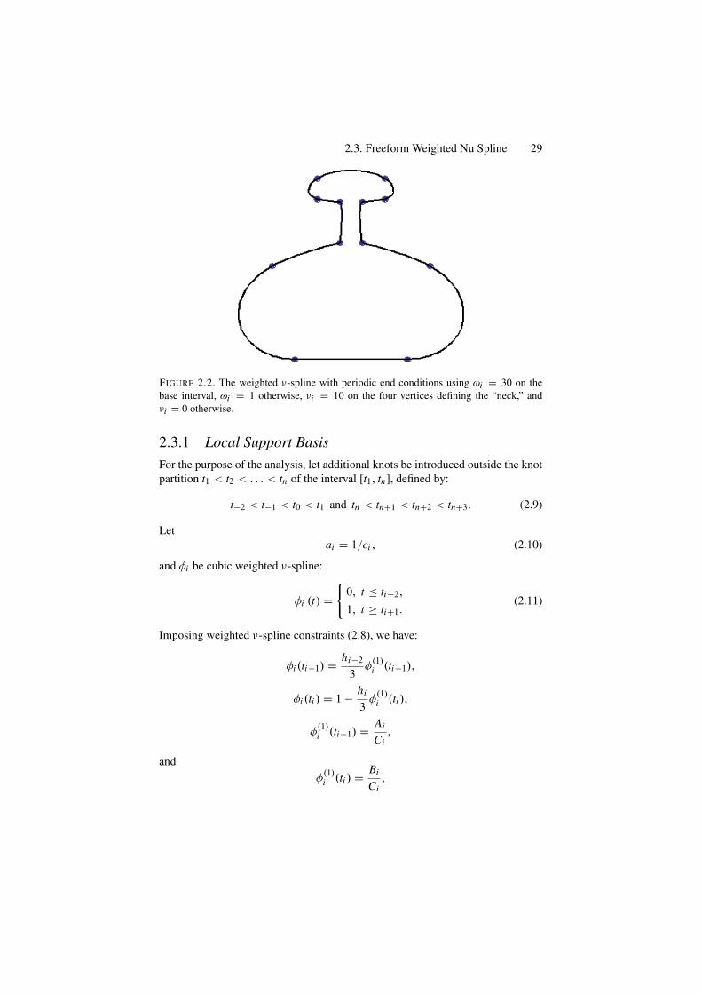
2.3. Freeform Weighted Nu Spline 29
FIGURE 2.2. The weighted ν-spline with periodic end conditions using ωi = 30 on thebase interval, ωi = 1 otherwise, νi = 10 on the four vertices defining the “neck,” andνi = 0 otherwise.
2.3.1 Local Support BasisFor the purpose of the analysis, let additional knots be introduced outside the knotpartition t1 < t2 < . . . < tn of the interval [t1, tn], defined by:
t−2 < t−1 < t0 < t1 and tn < tn+1 < tn+2 < tn+3. (2.9)
Letai = 1/ci , (2.10)
and φi be cubic weighted ν-spline:
φi (t) ={
0, t ≤ ti−2,
1, t ≥ ti+1.(2.11)
Imposing weighted ν-spline constraints (2.8), we have:
φi (ti−1) = hi−2
3φ
(1)i (ti−1),
φi (ti ) = 1 − hi
3φ
(1)i (ti ),
φ(1)i (ti−1) = Ai
Ci,
andφ
(1)i (ti ) = Bi
Ci,
30 2. Weighted Nu Splines
where, if di = 12 ai ai−1νi + ai−1 + ai , then
Ai = 3ai−2
hi−1di ,
Bi = 3ai
hi−1di−1,
Ci = di di−1 + ai
hi−1(hi−1 + hi )di−1 + ai−2
hi−1(hi−1 + hi−2)di .
Let
Di = hi−1di di−1 + ai (hi−1 + hi )di−1 + ai−2(hi−1 + hi−2)di ,
µi = φi+1(ti ), λi = 1 − φi (ti ),
µi = φ(1)i+1(ti ), λi = φ
(1)i (ti ),
Then
λi = 3ai di−1
Di, µi = 3ai−1di+1
Di+1,
µi = hi−1
3µi , λi = hi
3λi ,
and hence0 ≤ µi ≤ 1, 0 ≤ λi ≤ 1 and 0 ≤ µi + λi ≤ 1.
Now defineBi (t) = φi (t) − φi+1(t).
Then Bi has the local support (ti−2, ti+2) and an explicit representation of B jon any interval (ti , ti+1) (in particular, for i = j − 2, j − 1, j, j + 1) can becalculated as:
B j (t) = (1 − θ)3 B j (ti ) + θ(1 − θ)2(3B j (ti )hi B(1)j (ti ))
+ θ2(1 − θ)(3B j (ti+1) − hi B(1)j (ti+1)) + θ3 B j (ti+1), (2.12)
whereB j (ti ) = B(1)
j (ti ) = 0 for i = j − 1, j, j + 1,
andB j (t j−1) = µ j−1, B(1)
j (t j−1) = µ j−1,
B j (t j ) = 1 − λ j − µ j , B(1)j (t j ) = λ j − µ j ,
B j (t j+1) = λ j+1, B(1)j (t j+1) = −λ j+1.
⎫⎪⎪⎬
⎪⎪⎭(2.13)
Careful examination of the Bezier vertices of B j (t) in (2.12) shows these to benon-negative for νi , ωi satisfying (2.7) and thus B j (t) ≥ 0, ∀t . This leads to thefollowing:
2.3. Freeform Weighted Nu Spline 31
Proposition 2.1. The local support basis functions (2.12) are such that the foll-owing properties hold:
(i) (Local support) B j (t) = 0 for t /∈ (t j−2, t j+2),
(ii) (Partition of unity)n+1∑
j=−1B j (t) = 1 for t ∈ [t1, tn],
(iii) (Positivity) B j (t) ≥ 0 for all t .
2.3.2 Design CurveNow, we need a convenient method to compute the curve representation. It isdesired to apply the above developed local basis functions to develop a freeformweighted ν-spline curve as follows:
P(t) =n+1∑
j=−1
B j (t)Pj , t ∈ [t1, tn], (2.14)
where Pj ∈ RN , j = 0, 1, . . . , n + 1, define the control points of the representa-tion. By the local support property,
P(t) =i+2∑
j=i−1
B j (t)Pj , t ∈ [ti , ti+1), i = 0, . . . , n − 1.
Substitution of (2.12), t ∈ [ti , ti+1), then gives the piecewise defined Bezier rep-resentation
P(t) ≡ Pi (t) = Fi (1 − θ)3 + 3θ(1 − θ)2Vi + 3θ2(1 − θ)Wi + Fi+1θ3, (2.15)
whereFi = λi Pi−1 + (1 − λi − µi )Pi + µi Pi+1,Vi = (1 − αi )Pi + αi Pi+1,Wi = βi Pi + (1 − βi )Pi+1,
⎫⎬
⎭(2.16)
with
αi = µi + hi µi/3 = µi
3(hi−1 + hi ),
βi = λi+1 + hi∧λi = λi+1
3(hi + hi+1).
This transformation to Bezier form is very convenient for computational purposesand also leads to the following:
Proposition 2.2. (Variation Diminishing Property) The weighted ν-spline curveP(t), t ∈ [t0,tn], defined by (2.14), crosses any (hyper) plane of dimension N − 1no more times than it crosses the “control polygon” joining the control pointsP−1, P0, . . . , Pn+1.
32 2. Weighted Nu Splines
Proof. Following the arguments of positivity in the previous proposition, it isstraightforward that 0 ≤ αi ≤ 1, 0 ≤ βi ≤ 1, and 0 ≤ αi + βi ≤ 1. Thus, Vi andWi lie on the line segment joining Pi and Pi+1, where Vi is before Wi . It can alsobe simply noted that
Fi = (1 − γi )Wi−1 + γi Vi , (2.17)
where0 < γi = hi−1
hi−1 + hi< 1.
Thus, the control polygon of the piecewise defined Bezier representation isobtained by corner cutting of the weighted ν-spline control polygon. Since thepiecewise defined Bezier representation is variation diminishing, it follows thatweighted ν-spline representation is variation diminishing.
2.3.3 Shape ControlThe shape parameters, defined in (2.7), can be used to control the local orglobal shape of the design curve. To analyze such behaviors, the explicit formon (2.ti , ti+1) of the weighted ν-spline design curve (2.14) can be expressed as:
P(t) = li (t) + ei (t), (2.18)
whereli (t) = (1 − θ)Fi + θ Fi+1, (2.19)
and
ei (t) = θ(1 − θ){[
(Fi+1 − Fi ) − hi P(1)(ti )](θ − 1)
+[(Fi+1 − Fi ) − hi P(1)(ti+1)
]θ}
. (2.20)
Proposition 2.3. Let ωi = ω ≥ 1, and νi = 0,∀i are all bounded then theweighted ν-spline design curve is straightway the standard cubic spline.
Proof. It follows from the last constraint of relation (2.8).
Proposition 2.4. (Global Tension) Let ωi ≥ 1, ∀i , be bounded and νi ≥ ν thenthe weighted ν-spline curve (2.14) converges uniformly to the control polygonP0, . . ., Pn as ν → ∞.
Proof. Let νi = ν, ∀i then from (2.1)
limν→∞ P(1)(ti ) = 0. (2.21)
Moreoverlim
ν→∞ µi = 0 = limν→∞ λi , ∀i.
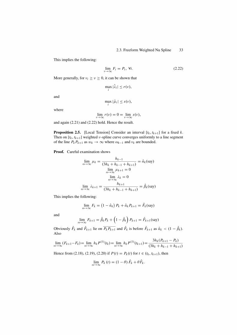
2.3. Freeform Weighted Nu Spline 33
This implies the following:
limν→∞ Fi = Pi , ∀i. (2.22)
More generally, for νi ≥ ν ≥ 0, it can be shown that
maxi
|λi | ≤ r(ν),
andmax
i|µi | ≤ s(ν),
wherelim
ν→∞ r(ν) = 0 = limν→∞ s(ν),
and again (2.21) and (2.22) hold. Hence the result.
Proposition 2.5. [Local Tension] Consider an interval [tk, tk+1] for a fixed k.Then on [tk, tk+1] weighted ν-spline curve converges uniformly to a line segmentof the line Pk Pk+1 as wk → ∞ where ωk−1 and νk are bounded.
Proof. Careful examination shows
limω→∞ µk = hk−1
(3hk + hk−1 + hk+1)= αk(say)
limω→∞ µk+1 = 0
limω→∞ λk = 0
limω→∞ λk+1 = hk+1
(3hk + hk−1 + hk+1)= βk(say)
This implies the following:
limω→∞ Fk = (1 − αk
)Pk + αk Pk+1 = Fk(say)
andlim
ω→∞ Fk+1 = βk Pk +(
1 − βk
)Pk+1 = Fk+1(say)
Obviously Fk and Fk+1 lie on Pk Pk+1 and Fk is before Fk+1 as αk < (1 − βk).Also
limω→∞(Fk+1−Fk)= lim
ω→∞ hk P(1)(tk)= limω→∞ hk P(1)(tk+1)= 3hk(Pk+1 − Pk)
(3hk + hk−1 + hk+1)
Hence from (2.18), (2.19), (2.20) if P(t) = Pk(t) for t ∈ (tk, tk+1), then
limω→∞ Pk (t) = (1 − θ) Fk + θ Fk .
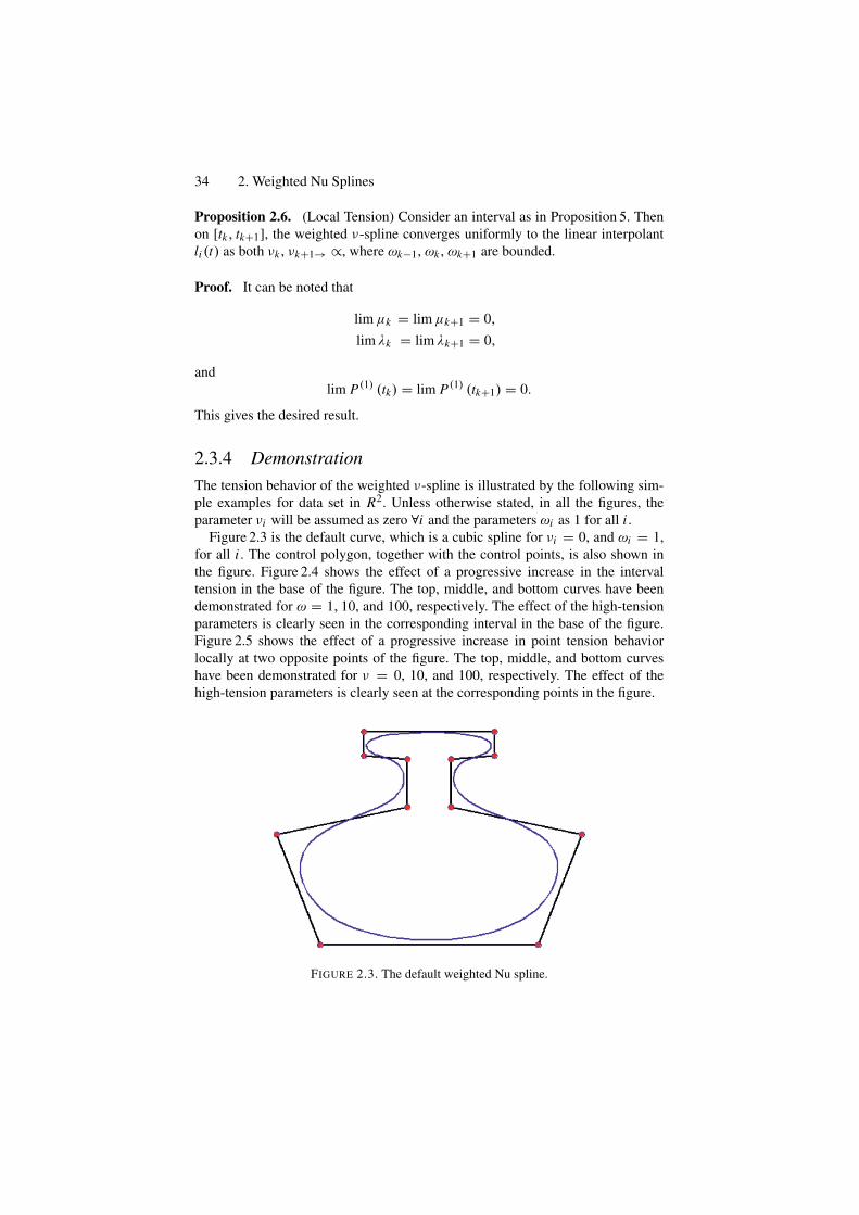
34 2. Weighted Nu Splines
Proposition 2.6. (Local Tension) Consider an interval as in Proposition 5. Thenon [tk, tk+1], the weighted ν-spline converges uniformly to the linear interpolantli (t) as both νk , νk+1→ ∝, where ωk−1, ωk , ωk+1 are bounded.
Proof. It can be noted that
lim µk = lim µk+1 = 0,
lim λk = lim λk+1 = 0,
andlim P(1) (tk) = lim P(1) (tk+1) = 0.
This gives the desired result.
2.3.4 DemonstrationThe tension behavior of the weighted ν-spline is illustrated by the following sim-ple examples for data set in R2. Unless otherwise stated, in all the figures, theparameter νi will be assumed as zero ∀i and the parameters ωi as 1 for all i .
Figure 2.3 is the default curve, which is a cubic spline for νi = 0, and ωi = 1,for all i . The control polygon, together with the control points, is also shown inthe figure. Figure 2.4 shows the effect of a progressive increase in the intervaltension in the base of the figure. The top, middle, and bottom curves have beendemonstrated for ω = 1, 10, and 100, respectively. The effect of the high-tensionparameters is clearly seen in the corresponding interval in the base of the figure.Figure 2.5 shows the effect of a progressive increase in point tension behaviorlocally at two opposite points of the figure. The top, middle, and bottom curveshave been demonstrated for ν = 0, 10, and 100, respectively. The effect of thehigh-tension parameters is clearly seen at the corresponding points in the figure.
FIGURE 2.3. The default weighted Nu spline.
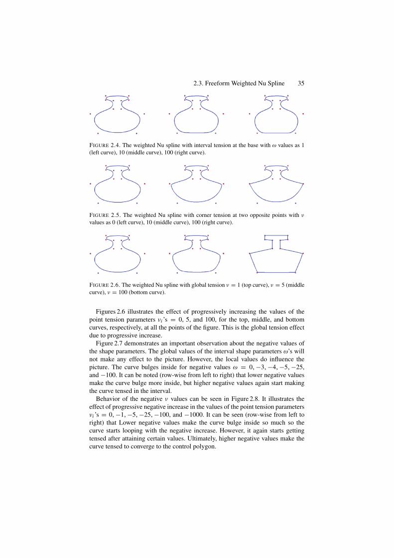
2.3. Freeform Weighted Nu Spline 35
FIGURE 2.4. The weighted Nu spline with interval tension at the base with ω values as 1(left curve), 10 (middle curve), 100 (right curve).
FIGURE 2.5. The weighted Nu spline with corner tension at two opposite points with νvalues as 0 (left curve), 10 (middle curve), 100 (right curve).
FIGURE 2.6. The weighted Nu spline with global tension ν = 1 (top curve), ν = 5 (middlecurve), ν = 100 (bottom curve).
Figures 2.6 illustrates the effect of progressively increasing the values of thepoint tension parameters νi ’s = 0, 5, and 100, for the top, middle, and bottomcurves, respectively, at all the points of the figure. This is the global tension effectdue to progressive increase.
Figure 2.7 demonstrates an important observation about the negative values ofthe shape parameters. The global values of the interval shape parameters ω’s willnot make any effect to the picture. However, the local values do influence thepicture. The curve bulges inside for negative values ω = 0,−3,−4,−5,−25,and −100. It can be noted (row-wise from left to right) that lower negative valuesmake the curve bulge more inside, but higher negative values again start makingthe curve tensed in the interval.
Behavior of the negative ν values can be seen in Figure 2.8. It illustrates theeffect of progressive negative increase in the values of the point tension parametersνi ’s = 0,−1,−5,−25,−100, and −1000. It can be seen (row-wise from left toright) that Lower negative values make the curve bulge inside so much so thecurve starts looping with the negative increase. However, it again starts gettingtensed after attaining certain values. Ultimately, higher negative values make thecurve tensed to converge to the control polygon.
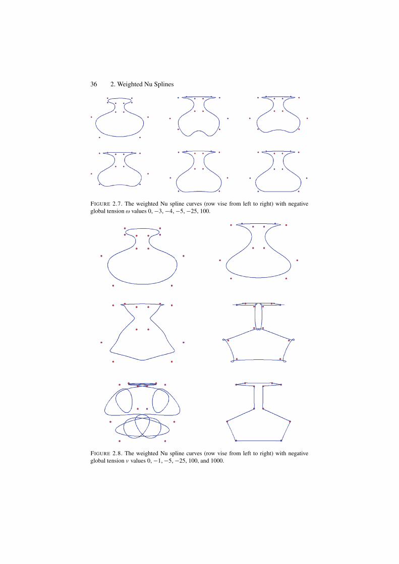
36 2. Weighted Nu Splines
FIGURE 2.7. The weighted Nu spline curves (row vise from left to right) with negativeglobal tension ω values 0, −3, −4, −5, −25, 100.
FIGURE 2.8. The weighted Nu spline curves (row vise from left to right) with negativeglobal tension ν values 0, −1, −5, −25, 100, and 1000.
2.4. Surfaces 37
2.3.5 Advantages and FeaturesThe method has various advantages and features as follows:
• It enjoys the good features of cubic splines.• It enjoys all the standard geometric properties of B-splines.• The method is geometrically smooth.• It recovers the cubic B-spline method as a special case.• It recovers the weighted spline method as a special case.• It recovers the Nu-spline method as a special case.• It possesses interested shape design features.• It has two families of shape parameters working in such a way that one family
of parameters is associated with intervals and the other with points. These para-meters provide a variety of shape controls such as point and interval tension.
• Negative weights can also be utilized for shape design.• It is computationally economical because it consumes the cubic function only.• The method of evaluation is suggested by a transformation to Bezier form,
which is computable by any well-known recursive method too.• In addition to direct manipulation, the interpolation method can be computed
through B-spline-like formulation too. This point will be discussed in detailsomewhere else later.
• The curve method is extendable to surfaces. The direct approach using a tensorproduct is the simplest one.
2.4 Surfaces
The extension of the curve scheme, to tensor product surface representations:
P(t, t) =m+1∑
i=−1
n+1∑
j=−1
Pi, j Bi (t)B j (t),
where t−2 ≤ t ≤ tm+3, t−2 ≤ t ≤ tn+3, is immediately apparent. This surfacepresents a bicubic weighted ν-spline surface with shape parameters as:
vi ≥ 0, i = 1, . . . , m, wi > 0, i = 1, . . . , m − 1,
ν j ≥ 0, j = 1, . . . , n, ω j > 0, j = 1, . . . , n − 1.
HerePi, j ∈ R3, i = −1, . . . , m + 1, j = −1, . . . , n + 1.
are the data points and Bi , i = −1, . . . , m + 1 and B j , j = −1, . . . , n + 1 arethe local support bases functions for the weighted ν-spline in t and t directions,respectively. However, this representation exhibits a problem common to all tensorproduct descriptions in that the shape control parameters now affect a completerow or column of the tensor product array.
38 2. Weighted Nu Splines
Nielson [12] solves this problem for his cubic ν-spline representation byconstructing a Boolean sum, spline-blended, rectangular network of parametricν-spline curves. Another possibility is to allow the shape parameters to be variablein the orthogonal direction to, for example, the local support basis functions of thetensor product form.
We propose a tensor product like the approach in [16,17], but actually it is not atensor product. Instead of step functions, the tension weights are introduced as C2
continuous cubic B-splines in the description of the tensor product. This produceslocal control in the construction of surfaces in an independent way. The detailsof the proposed method are out of the scope of this paper and will be discussedelsewhere.
2.5 Summary
A freeform C1 weighted Nu spline curve design has been developed throughthe construction of local support B-spline-like basis functions. This cubic splinemethod has been developed with a view to its application in computer graphics,geometric modeling, and CAGD. It is quite reasonable to construct a freeformcubic spline method, which involves two families of shape parameters in exactlya similar way as in interpolatory weighted ν-spline. These parameters provide avariety of local and global shape controls such as interval and point shape effects.The visual smoothness of the proposed method is also C1, which is same asthe smoothness of interpolatory weighted ν-spline. The freeform C1 weightedNu-spline method can be applied to tensor product surfaces, but unfortunately,in the context of interactive surface design, this tensor product surface is not thatuseful because any one of the tension parameters controls an entire correspondinginterval strip of the surface. Thus, as an application of C1 spline for the surfaces, amethod similar to Nielson’s [12] spline blended methods may be attempted. Thiswill produce local shape control, which is quite useful regarding the computergraphics and geometric modeling applications.
2.6 Exercises
1. Write a program to implement the curve design method in Section 2.2.2. Write a program to implement the curve design method in Section 2.3.3. Check the difference of shape effects in your programs of Exercise 2.6.1 and
2.6.2 when the schemes are implemented in scalar form.
References1. Barsky, B.A. (1981), The Beta-Spline: A Local Representation Based on Shape Para-
meters and Fundamental Geometric Measure, Ph.D. Thesis, University of Utah.
References 39
2. Bartels, R., and Beatty, J. (1984), Beta-splines with a difference, Technical ReportCS-83-40, Computer Science Department, University of Waterloo, Waterloo, Canada.
3. Boehm, W. (1985), Curvature continuous curves and surfaces, Comp Aided GeomDesign 2(2), 313–323.
4. Cline, A. (1974), Curve fitting in one and dimensions using splines under tension,Comm ACM 17, 218–223.
5. Dierckx, P., and Tytgat, B. (1989), Generating the Bezier points of β-spline curve,Comp Aided Geom Design 6, 279–291.
6. Farin, G.E. (1996), Curves and Surfaces for CAGD, Academic Press, New York.7. Foley, T.A. (1987), Local control of interval tension using weighted splines. Comp
Aided Geom. Design 3, 281–294.8. Foley, T.A. (1987), Interpolation with interval and point tension controls using cubic
weighted ν-splines, ACM Trans Math Software 13, 68–96.9. Goodman, T.N.T., and Unsworth, K. (1985), Generation of Beta spline curves
using a recursive relation. In: Fundamental Algorithms for Computer Graphics.R.E. Earnshaw (Ed.), Springer-Verlag, Berlin, pp. 326–357.
10. Lewis, J. (1975), “B-spline” bases for splines under tension, Nu-splines, and frac-tional order splines, Presented at the SIAM-SIGNUM Meeting, San Francisco, CA.
11. Nielson, G.M. (1974), Some piecewise polynomial alternatives to splines under ten-sion, In: Computer-Aided Geometric Design, R.F. Barnhill (Ed.), Academic Press.New York.
12. Nielson, G.M. (1986), Rectangular ν-splines. IEEE Comp Graph Appl 6, 35–40.13. Pruess, S. (1979), Alternatives to the exponential spline in tension, Math Comp 33,
1273–1281.14. Salkauskas, K. (1984), C1 splines for interpolation of rapidly varying data, Rocky Mtn
J Math 14, 239–250.15. Sarfraz, M. (1992), A C2 rational cubic spline alternative to the NURBS, Comp &
Graph 16(l), 69–78.16. Sarfraz, M. (1995), Curves and surfaces for CAD using C2 rational cubic splines,
Int J Eng Comput, Springer-Verlag, 11(2), 94–102.17. Sarfraz, M. (1994), Freeform rational bicubic spline surfaces with tension control,
Facta Universitatis (NIS), Ser Math Informatics, 9, 83–93.18. Sarfraz, M. (1994), Cubic spline curves with shape control, Int J Comput Graphics,
Elsevier Science, 18(5), 707–713.19. Sarfraz, M, (2003), Weighted Nu splines: an alternative to NURBS, Advances in Geo-
metric Modeling, Ed.: M. Sarfraz, John Wiley, pp. 81–95.20. Schoenburg, I. J. (1946), Contributions to the problem of approximation of equidistant
data by analytic functions, Appl Math 4, 45–99.21. Schweikert, D.G. (1966), An interpolation curve using a spline in tension, J Math Phys
45, 312–317.22. Sarfraz, M. (2004), Weighted Nu splines with local support basis functions, Int J Com-
put Graphics, Elsevier Science, 28(4), 539–549.
3Rational Cubic Spline with ShapeControl
Abstract. Interactive curve design is a basic need for CAD/CAM, computer graphics,vision, imaging and various other disciplines [1–28]. Having a robust, visually pleas-ant, well controlled, and effective scheme may be a useful solution to many problems inpractice. A rational spline with some shape parameters may be a good choice in this regard.This chapter has been devoted to a C2 rational spline scheme having interesting features.It is also an alternative to various other schemes, in the literature, like weighted spline,ν – spline, weighted Nu spline, and γ – spline, and so on. In addition to the interpolatoryversion, the spline is also presentable in B-spline-like form to produce freeform curves.
3.1 Introduction
A rational cubic spline with tension was described and analyzed by Gregory andSarfraz [23]. It provides a C2 computationally simpler alternative to the exponen-tial spline-under-tension of Schweikert [24], Cline [25] and Preuss [26] as well asan alternative to C1 and GC2 spline methods such as the weighted ν – spline ofFoley [8] and γ – spline of Boehm [3], and so on. Regarding shape characteristics,it has a shape control parameter associated with each interval which can be usedfor flatten or tighten the curve both locally and globally.
This chapter presents a description and analysis of a rational cubic spline thathas two shape parameters associated with each interval. The spline can be used incomputer graphics, CAGD, and CAD/CAM to represent the parametric curves ininterpolatory as well approximation (freeform) form. The rational spline not onlyrecovers the rational cubic spline with tension of Gregory and Sarfraz [23] butalso provides a C2 alternative to most of the existing C1 and GC2 spline methodssuch as the weighted splines of Foley [7], ν – spline of Nielson [11,12], weightedν – splines of Foley [8], γ – spline of Boehm [3], rational geometric splines ofBoehm [27], and so on.
The shape parameters of the rational spline can be utilized to achieve a varietyof shape controls such as biased, point and interval tensions. Since the spline isdefined on a nonuniform knot partition, the partition itself provides additional
41
42 3. Rational Cubic Spline with Shape Control
degrees of freedom on the curve. However, the parametrization is normallyexpected to be defined on a uniform known partition, or by cumulative chordlength, or by some other appropriate means.
The rational spline is based on a rational cubic Hermite interpolant which isintroduced in Section 3.2. together with some preliminary analysis. Section 3.3describes the rational spline and analyses of its behavior with respect to one shapeparameter in each interval while the generalization to two shape parameters isdiscussed in Section 3.4. Section 3.5 consists of some illustrative examples aboutthe interpolation spline. The survey of freeform curves is made in Section 3.6and B-spline-like bases are constructed in Section 3.8. Freeform design curve for-mulation is made in Section 3.9, whereas Section 3.10 explains the behavior ofshape parameters. Freeform curve scheme has been demonstrated in Section 3.11.A brief description of surfaces has been made in Sections 3.12 and 3.13.
3.2 C1 Piecewise Rational Cubic Hermite Interpolant
A piecewise rational cubic Hermite parametric function p ∈ C1 [t0, tn], with para-meters vi , wi , i = 0, . . . , n − 1, is defined for t ∈ [ti , ti+1
], i = 0, . . . , n − 1, by
p(t) = pi (ti ; vi , wi )
= (1 − θ)3 Fi + θ (1 − θ)2 (vi Fi + hi Di ) + θ2 (1 − θ) (wi Fi+1 − hi Di+1) + θ3 Fi+1
(1 − θ)3 + vi θ (1 − θ)2 + wiθ2 (1 − θ) + θ3
(3.1)
where the notations Fi , Di , ti , hi , θ are as mentioned in Section 1.3 and vi , wi ≥0.The function p (t)—see Figure 3.1—has the Hermite interpolation properties
thatp(ti ) = Fi and p(1)(ti ) = Di , i = 0, . . . , n. (3.2)
The vi and wi , i = 0, . . . , n − 1, will be used as shape parameters to control andfine tune the shape of the curve. The case vi = wi = 3, i = 0, . . . , n − 1 is thatof cubic Hermite interpolation and the restriction vi , wi ≥ 0 ensures a positivedenominator in Equation (3.1).
For vi , wi = 0, Equation (3.1) can be written in the form:
pi (ti ; vi , wi ) = R0(θ; vi , wi )Fi + R1 (θ; vi , wi ) Vi + R2 (θ; vi , wi ) Wi
+R3 (θ; vi , wi ) Fi+1, (3.3)
wherevi = Fi + hi Di/vi , Wi = Fi+1 − hi Di+1/wi , (3.4)
and R j (θ; vi , wi ), j = 0, 1, 2, 3, are appropriately defined rational functions with
3∑
j=0
R j (θ; vi , wi ) = 1. (3.5)
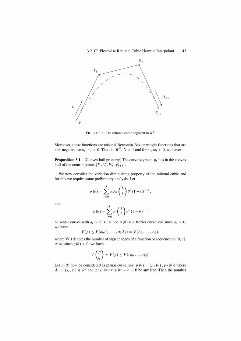
3.2. C1 Piecewise Rational Cubic Hermite Interpolant 43
Vi
Wi
Fi+1
Di+1
Di
Fi
FIGURE 3.1. The rational cubic segment in R2.
Moreover, these functions are rational Bernstein-Bezier weight functions that arenon-negative for vi , wi > 0. Thus, in RN , N > 1 and for vi , wi > 0, we have:
Proposition 3.1. (Convex hull property) The curve segment pi lies in the convexhull of the control points {Fi , Vi , Wi , Fi+1}.
We now consider the variation diminishing property of the rational cubic andfor this we require some preliminary analysis. Let
p (θ) =3∑
i=0
ai Ai
(3i
)θ i (1 − θ)3−i ,
and
q (θ) =3∑
i=0
ai
(3i
)θ i (1 − θ)3−i
be scalar curves with ai > 0,∀i . Since p (θ) is a Bezier curve and since ai > 0,we have
V (p) ≤ V (a0 A0, . . . , a3 A3) = V (A0, . . . , A3),
where V(.) denotes the number of sign changes of a function or sequence on [0, 1].Also, since q(θ) > 0, we have
V(
pq
)= V (p) ≤ V (A0, . . . , A3),
Let p (θ) now be considered as planar curve, say, p (θ) = (p1 (θ) , p2 (θ)) whereAi = (xi , yi ) ∈ R2 and let L ≡ ax + by + c = 0 be any line. Then the number
44 3. Rational Cubic Spline with Shape Control
of times the line L crosses the rational cubic curve p(θ)/q(θ) is the same as itcrosses the cubic Bezier curve p(θ), q(θ) > 0. This number is
V (ap1 + bp2 + c) = V(
a∑
ai xi
(3i
)θ i (1 − θ)3−i
+ b∑
ai yi
(3i
)θ i (1 − θ)3−i + c
)
= V(
a∑
xi
(3i
)θ i (1 − θ)3−i +b
∑yi
(3i
)θ i (1−θ)3−i
+ c∑(
3i
)θ i (1 − θ)3−i
)
= V(∑
(axi + byi + c)(
3i
)θ i (1 − θ)3−i
)
= the number of times the line L crosses the polygon A0, . . . , A3.
These arguments can be extended to rational curve of any degree in RN with anyhyper plane of dimension N − 1. Thus, we have:
Proposition 3.2. (Variation diminishing property) The curve segment pi crossesany (hyper) plane of dimension N − 1 no more times than it crosses the controlpolygon joining Fi , Vi , Wi , Fi+1.
Remark 3.3. In the scalar case when vi , wi ,= ri , the convex hull(Proposition 3.1) and variation diminishing (Proposition 3.2) properties applyto the curve segment (t, pi (t; ri , ri )) ∈ R2, t ∈ (ti , ti+1) with control points:
{(ti , Fi ) , (ti + hi/ri , Vi ) , (ti+1 − hi/ri , Wi ) , (ti+1, Fi+1)} . (3.6)
This is a consequence of the identity
t ≡ R0(θ; ri )ti + R1(θ; ri )(ti + hi/ri ) + R2(θ; ri )(ti+1 − hi/ri ) + R3(θ; ri )ti+1,(3.7)
whereRJ (θ; ri ) ≡ R j (θ; ri , ri ), j = 0, . . . , 3. (3.8)
In fact, (t, p(t)) can be considered as an application of the interpolation schemein R2 to the values (ti , Fi ) ∈ R2 and derivatives (1, Di ) ∈ R2, i = 0, . . . , n.
3.3 One-Parameter Rational Cubic Spline
For simplicity, in this section, let us assume vi = wi = ri say. The rational cubicin Equation (3.1) can then be expressed in the form:
pi (t; ri , ri ) = li (t) + ei (t; ri ), (3.9)
3.3. One-Parameter Rational Cubic Spline 45
where
li (t) = (1 − θ)Fi + θ Fi+1. (3.10)
ei (t; ri ) = hiθ(1 − θ) {(�i − Di )(θ − 1) + (�i − Di+1)θ}1 + (ri − 3)θ(1 − θ)
. (3.11)
This immediately leads to:
Proposition 3.4. (Interval tension property) For given fixed (or bounded)Di , Di+1 the rational cubic Hermite interpolant in Equation (3.10) convergesuniformly to the linear interplant in Equation (3.11) on
[ti , ti+1
]as ri → ∞ i.e.
limri →∞ ||ei || = lim
ri →∞ ||pi − li || = 0. (3.12)
Moreover, the component functions of ei tend to zero monotonically, bothuniformly and pointwise on
[ti , ti+1
].
Remark 3.5. The interval tension property can also be observed from the behav-ior of the control points Vi , Wi defined by Equation (3.4), and hence of theBernstein-Bezier convex hull, as ri → ∞.
Now we construct a C2 rational spline interpolant. This requires knowledge ofthe second derivative which, after some simplifications, is given by:
p(2)i (t; ri , ri ) = 2
{αi (1 − θ)3 + βiθ(1 − θ)2 + γiθ
2(1 − θ) + δiθ3}
hi {1 + (ri − 3)θ(1 − θ)}3 , (3.13a)
whereαi = ri (�i − Di ) − Di+1 + Di ,βi = 3(�i − Di ),γi = 3(Di+1 − �i ),δi = ri (Di+1 − �i ) − Di+1 − Di ).
⎫⎪⎪⎬
⎪⎪⎭(3.13b)
We now follow the familiar procedure of allowing the derivative parametersDi , i = 0, . . . , n to be degrees of freedom that are constrained by the impositionof C2 continuity conditions:
p(2)(ti+) = p(2) (ti−) , i = 1, . . . , n − 1. (3.14)
These C2 conditions give, form (3.13a) and (3.13b), the linear system of consis-tency equations as follows:
hi Di−1 + {hi (ri−1 − 1) + hi−1(ri − 1)} Di + hi−1 Di+1
= hiri−1�i−1 + hi−1ri�i , i = 1, . . . , n − 1, (3.15)
with appropriate end conditions D0 and Dn , Equations (3.15) is a tridiagonal linearsystem in the unknowns Di , i = 1, . . . , n − 1. Assume that
ri ≥ r > 2, (3.16)
46 3. Rational Cubic Spline with Shape Control
then the tridiagonal linear system, in Equations (3.15), is strictly diagonally dom-inant and hence has a unique solution that can be calculated easily by use of thetridiagonal LU decompositon algorithm. Thus a rational cubic spline interpolantcan be constructed with tension parameters ri , i = 0, . . . , n −1, where the specialcase ri = 3, i = 0, . . . , n − 1 corresponds to cubic spline interpolation. We nowexamine the behavior of the rational spline interpolant with respect to the tensionparameters ri in the following propositions.
Proposition 3.6. (Global tension property) Let l ∈ C0 [t0, tn] denote the piece-wise linear interpolant defined for t ∈ [
ti , ti+1]
by l(t) = li (t); see Equation(3.11). Suppose that ri ≥ r > 2, i = 0, . . . , n − 1, as in Equation (3.16). Then therational spline interpolant converges uniformly to l as r → ∞, i.e., on [t0, tn],
limr→∞ ||p − l|| = 0. (3.17)
Proof. Suppose ri = r, i = 0, . . . , n − 1, then from Equations (3.15), it followsthat
limr→∞ Di = (hi�i−1 + hi−1�i )
hi + hi−1, i = 1, . . . , n − 1. (3.18)
More generally, for ri satisfying (3.16), it can be shown that
max1≤i≤n−1
||Di ||∞ ≤ max {||�||∞r/(r − 2), ||D0||, ||Dn||} , (3.19)
where||�|| = max
1≤i≤n−1||�i ||∞. (3.20)
Hence the solution Di , i = 1, . . . , n − 1 of the consistency Equations (3.15)is bounded with respect to r . Now, from Equation (3.12), the tension propertyin Equation (3.12) of Proposition 3.4 can clearly be extended to the case ofbounded r . Thus applying Equation (3.12) on each interval gives the desired resultin Equation (3.17). �
Proposition 3.7. (Local tension property) Let ri ≥ r > 2,∀i and consider aninterval
[tk, tk+1
]for a fixed k ∈ {0, . . . , n − 1}. Then, on
[tk, tk+1
]the rational
spline interpolant converges uniformly to the line segment lk as rk → ∞ i.e.
limrk→∞ ‖pk − lk‖ = 0. (3.21)
Proof. The boundedness property in Equation (3.19) holds as in Proposition 3.6(where we can assume the additional constraints rk ≥ r > 2 to the hypothesescurrently being imposed. Thus, Equation (3.12) applies for the case i = k. �
Remark 3.8. In Proposition 3.7, there is no assumption that the ri , i = k are con-stant with respect to the limit process. However, in the case of constant ri , i = k,an analysis of the linear system in Equation (3.15) shows that
limrk→∞ ||Dk − �k ||∞ = lim
rk→∞ ||Dk+1 − �k ||∞ = 0. (3.22)
3.3. One-Parameter Rational Cubic Spline 47
This property reinforces the rate of convergence to zero of ek = pk−lk in Equation(3.21), as can be seen from Equation (3.12) with i = k. The following propositionshows that the influence of rk in this case has an exponential decay away from theinterval
[tk − tk+1
].
Proposition 3.9. (Exponential decay property) Let Di , i = 1, . . . , n − 1, denotethe solution of the consistency equations with tension parameters rk ≥ r > 2, i =0, . . . , n − 1, and let Di , i = 1, . . . , n − 1, denote the solution with parametersri ≥ r > 2, i = 0, . . . , n − 1, where ri = ri for i = k. Consider a knot ti , i ∈{0, . . . , n − 1}, where i = k − l or k + 1 + l, and l is a positive integer. Then
||Di − Di ||∞ ≤ 4γ l(1 + 2γ )
1 − γ||�||∞, (3.23a)
where ||�||∞ is the constant defined in Equation (3.20) and
γ = 1/(r − 1) < 1.
(Thus, for example, if r = 3 then γ = 1/2.)
Proof. To prove this result, let the consistency equations (3.15) be divided by thecoefficient of Di to give the matrix form
(l + F) D = B
where DT = D1, . . . , Dn−1 and the given end conditions D0 and Dn have beentransferred to the right-hand side B. Then F is a tridiagonal matrix such that
||F ||∞ ≤ 1r − 1
= γ
Also it can be shown that||B||∞ ≤ 2||�||∞
Similarly, for the perturbed system
(1 + F)D = B
where rk = rk + σ , we have
||F ||∞ ≤ 1r − 1
= γ and ||B||∞ ≤ 2||�||∞Now
D − D = ((1 + F)−1 − (1 + F)−1)B + (1 + F)−1[B − B]and we consider each of the terms of the right-hand side separately.
48 3. Rational Cubic Spline with Shape Control
Firstly, F and F are tridiagonal matrices that agree in rows l ≤ i ≤ k − 1 andk +2 ≤ i ≤ n −1 (i.e., only the kth and k +1st rows are changed by a perturbationof rk .) Thus, Fl and Fl agree in rows l ≤ i ≤ k − 1 and k + 1 + l ≤ i ≤ n − 1.Hence
ς = ((1 + F)−1 − (1 + F)−1)B =∞∑
ϑ=1
(−1)ϑ [Fϑ − Fϑ ]B
is such that the i th component, for i = k − l or i = k + l + 1 satisfies
ςi ≤∞∑
ϑ=l+1
(||F ||ϑ − ||F ||ϑ)||B|| ≤ γ l+1
1 − γ4||�||∞ (3.23b)
Secondly, we considerE = (1 + F)−1[B − B]
and apply an analysis that follows that of [Demko’77] (see his Proposition 3.1).Since F is tridiagonal, has bandwidth 2ϑ + 1 (i.e., the (i , j) elements are zero for|i − j | > ϑ). Hence for |i − j | = 1, the (i , j) element of the series expansion(1 + F)−1 =∑ (−1)ϑ Fϑ is not influenced by Fϑ for ϑ < l. Thus:
|| fi, j || ≤∞∑
ϑ=l+1
||F ||ϑ ≤ γ l
1 − γf or |i − j | = l
Finally, and B agree in rows l ≤ i ≤ k − 1 and k + 1 ≤ i ≤ n − 1. Hence the i thcomponent of E satisfies
|ei | = | fi,k(bk − bk) + fi,k+1(bk+1 − bk+1)| (3.23c)
≤⎧⎨
⎩
γ l
1−γ (|bk | + |bk |) + γ l+1
1−γ (|bk+1| + |bk+1)
γ l+1
1−γ (|bk | + |bk |) + γ l+1
1−γ (|bk+1| + |bk+1)
≤{
γ l (1+γ )1−γ 4 ‖�‖∞
Combination (3.23b) and (3.23c) then gives the desired result (3.23a). �
Remark 3.10. We note that
(i) the rational spline exists uniquely for ri ≥ r > 2(ii) the case ri = 3, i = 0, . . . , n − 1 is that of the cubic spline and
(iii) increasing ri tightens the curve both locally and globally (c.f. Propostions 3.6and 3.7. For the range 2 < ri < 3 the rational spline produces a more flexible,i.e. looser, curve than the cubic spline curve, both locally and globally.
3.4. Two-Parameter Rational Cubic Spline 49
3.4 Two-Parameter Rational Cubic Spline
In this section we generalize the curve representation of Section 3.3 and considerthe Hermite interpolant in Equation (3.1) of Section 3.2 for rational spline anlaysisand representation. We assume the shape parameters vi , wi > 0 as
vi = biwi , i = 0, . . . , n − 1, (3.24)
where 0 < bi < ∞.
Remark 3.11. For given fixed (or bounded) Di and Di+1, the following observa-tions can be made immediately from the Bernstein-Bezier representation (Equa-tion (3.3)) and the control points Vi , Wi defined by Equation (3.4), that:
(i) if wi → ∞, then the rational cubic Hermite interpolant (3.1) converges to therational linear interpolant Li (t, bi ) where
Li (t, bi ) = (1 − θ)bi Fi + θ Fi+1
(1 − θ)bi + θ, (3.25)
(ii) if bi > 1, i.e., vi exceeds wi , then the curve is pulled towards Fi in the interval[ti , ti+1
].
(iii) if bi = 1, i.e., vi = wi then increase in wi pulls the curve toward Fi and Fi+1the interval
[ti , ti+1
](see Proposition 4).
(iv) if 0 < bi < 1, i.e., wi exceeds vi then the curve is pulled toward Fi+1 in theinterval
[ti , ti+1
].
Now we proceed to construct a C2 rational spline interpolant. For this we are inof the second derivative values of Equation (3.1) at the knots. After some simpli-fications, we have
p(2)i (ti ; vi , wi ) = 2
[wi∆i − Di+1 + (1 − vi )Di
]hi ,
p(2)i (ti+1; vi , wi ) = 2
[−vi∇i + (wi − 1)Di+1 + Di]
hi .
}
(3.26)
C2 continuity condition at the knots ti , i = 1, . . . , n − 1, together with the infor-mation in Equation (3.26), lead to the following linear system of consistencyequations in the unknowns Di , i = 0, . . . , n:
hi Di−1 + {hi (wi−1 − 1) + hi−1(vi − 1)} Di + hi−1 Di+1
= hivi−1∇i−1 + hi−1wi∇i , i = 1, . . . , n − 1. (3.27)
With appropriate end conditions D0 and Dn and the assumption
vi , wi > 2, i = 0, . . . , n − 1, (3.28)
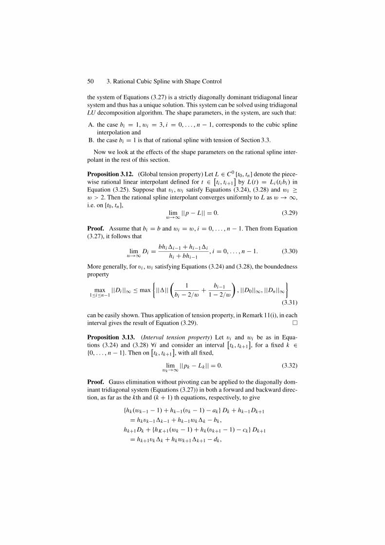
50 3. Rational Cubic Spline with Shape Control
the system of Equations (3.27) is a strictly diagonally dominant tridiagonal linearsystem and thus has a unique solution. This system can be solved using tridiagonalLU decomposition algorithm. The shape parameters, in the system, are such that:
A. the case bi = 1, wi = 3, i = 0, . . . , n − 1, corresponds to the cubic splineinterpolation and
B. the case bi = 1 is that of rational spline with tension of Section 3.3.
Now we look at the effects of the shape parameters on the rational spline inter-polant in the rest of this section.
Proposition 3.12. (Global tension property) Let L ∈ C0 [t0, tn] denote the piece-wise rational linear interpolant defined for t ∈ [
ti , ti+1]
by L(t) = Li (ti bi ) inEquation (3.25). Suppose that vi , wi satisfy Equations (3.24), (3.28) and wi ≥w > 2. Then the rational spline interpolant converges uniformly to L as w → ∞,i.e. on [t0, tn],
limw→∞ ||p − L|| = 0. (3.29)
Proof. Assume that bi = b and wi = w, i = 0, . . . , n − 1. Then from Equation(3.27), it follows that
limw→∞ Di = bhi�i−1 + hi−1�i
hi + bhi−1, i = 0, . . . , n − 1. (3.30)
More generally, for vi , wi satisfying Equations (3.24) and (3.28), the boundednessproperty
max1≤i≤n−1
||Di ||∞ ≤ max{||�||
(1
bi − 2/w+ bi−1
1 − 2/w
), ||D0||∞, ||Dn||∞
}
(3.31)
can be easily shown. Thus application of tension property, in Remark 11(i), in eachinterval gives the result of Equation (3.29). �
Proposition 3.13. (Interval tension property) Let vi and wi be as in Equa-tions (3.24) and (3.28) ∀i and consider an interval
[tk, tk+1
], for a fixed k ∈
{0, . . . , n − 1}. Then on[tk, tk+1
], with all fixed,
limwk→∞ ||pk − Lk || = 0. (3.32)
Proof. Gauss elimination without pivoting can be applied to the diagonally dom-inant tridiagonal system (Equations (3.27)) in both a forward and backward direc-tion, as far as the kth and (k + 1) th equations, respectively, to give
{hk(wk−1 − 1) + hk−1(vk − 1) − ak} Dk + hk−1 Dk+1
= hkvk−1�k−1 + hk−1wk�k − bk,
hk+1 Dk + {hK+1(wk − 1) + hk(vk+1 − 1) − ck} Dk+1
= hk+1vk�k + hkwk+1�k+1 − dk,
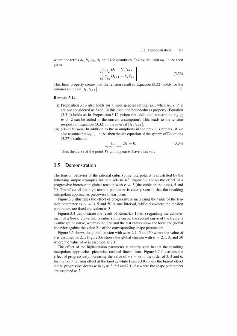
3.5. Demonstration 51
where the terms ak, bk, ck, dk are fixed quantities. Taking the limit wk → ∞ thengives
limwk→∞ Dk = ∇k/bk,
limwk→∞ Dk+1 = bk∇k,
⎫⎬
⎭(3.33)
This limit property means that the tension result in Equation (3.32) holds for therational spline on
[tk, tk+1
]. �
Remark 3.14.
(i) Proposition 3.13 also holds for a more general setting, i.e., when wi , i = kare not considered as fixed. In this case, the boundedness property (Equation(3.31)) holds as in Proposition 3.12 (when the additional constraints wk ≥w > 2 can be added in the current assumption). This leads to the tensionproperty in Equation (3.32) in the interval
[tk, tk+1
].
(ii) (Point tension) In addition to the assumptions in the previous remark, if wealso assume that wk−1 → ∞, then the kth equation of the system of Equations(3.27) results as:
limvk ,wk−1→∞ Dk = 0. (3.34)
Thus the curve at the point Pk will appear to have a corner.
3.5 Demonstration
The tension behavior of the rational cubic spline interpolants is illustrated by thefollowing simple examples for data sets in R2. Figure 3.2 shows the effect of aprogressive increase in global tension with r = 3 (the cubic spline case), 5 and50. The effect of the high-tension parameter is clearly seen in that the resultinginterpolant approaches piecewise linear form.
Figure 3.3 illustrates the effect of progressively increasing the value of the ten-sion parameter as r4 = 3, 5 and 50 in one interval, while elsewhere the tensionparameters are fixed equivalent to 3.
Figures 3.4 demonstrate the result of Remark 3.10 (iii) regarding the achieve-ment of a looser curve than a cubic spline curve; the second curve of the figure isa cubic spline curve, whereas the first and the last curves show the local and globalbehavior against the value 2.1 of the corresponding shape parameters.
Figure 3.5 shows the global tension with w = 2.1, 5 and 50 where the value ofv is assumed as 2.1; Figure 3.6 shows the global tension with v = 2.1, 3, and 50where the value of w is assumed as 2.1.
The effect of the high-tension parameter is clearly seen in that the resultinginterpolant approaches piecewise rational linear form. Figure 3.7 illustrates theeffect of progressively increasing the value of w3 = v4 in the order of 3, 4 and 6,for the point tension effect at the knot t4 while Figure 3.8 shows the biased effectdue to progressive decrease in v4 as 3, 2.5 and 2.1; elsewhere the shape parametersare assumed as 3.
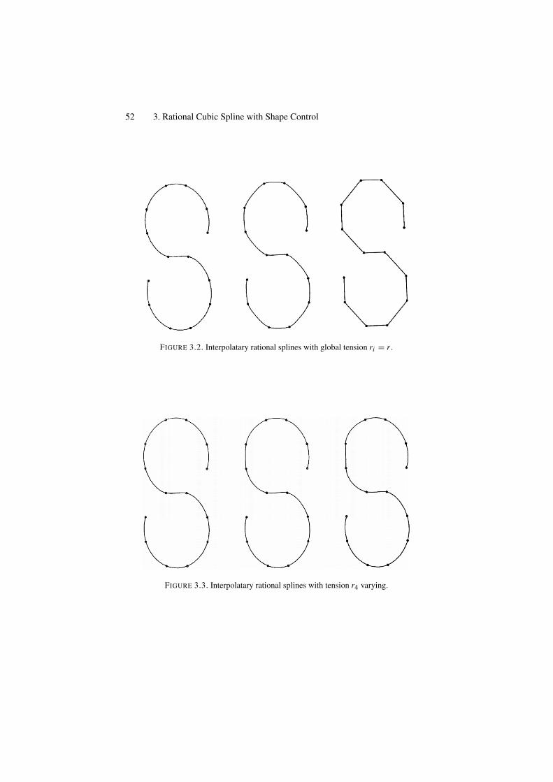
52 3. Rational Cubic Spline with Shape Control
FIGURE 3.2. Interpolatary rational splines with global tension ri = r .
FIGURE 3.3. Interpolatary rational splines with tension r4 varying.
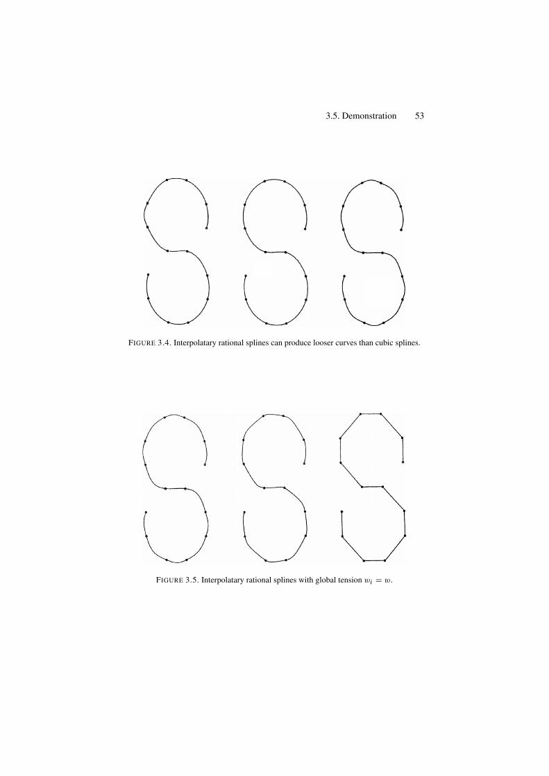
3.5. Demonstration 53
FIGURE 3.4. Interpolatary rational splines can produce looser curves than cubic splines.
FIGURE 3.5. Interpolatary rational splines with global tension wi = w.
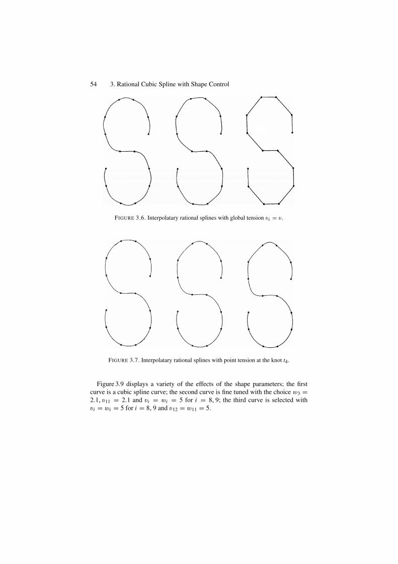
54 3. Rational Cubic Spline with Shape Control
FIGURE 3.6. Interpolatary rational splines with global tension vi = v .
FIGURE 3.7. Interpolatary rational splines with point tension at the knot t4.
Figure 3.9 displays a variety of the effects of the shape parameters; the firstcurve is a cubic spline curve; the second curve is fine tuned with the choice w3 =2.1, v11 = 2.1 and vi = wi = 5 for i = 8, 9; the third curve is selected withvi = wi = 5 for i = 8, 9 and v12 = w11 = 5.
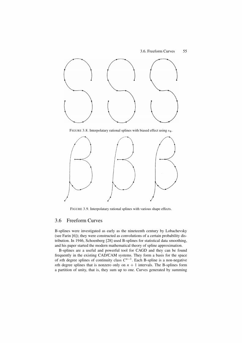
3.6. Freeform Curves 55
FIGURE 3.8. Interpolatary rational splines with biased effect using v4.
FIGURE 3.9. Interpolatary rational splines with various shape effects.
3.6 Freeform Curves
B-splines were investigated as early as the nineteenth century by Lobachevsky(see Farin [6]); they were constructed as convolutions of a certain probability dis-tribution. In 1946, Schoenberg [28] used B-splines for statistical data smoothing,and his paper started the modern mathematical theory of spline approximation.
B-splines are a useful and powerful tool for CAGD and they can be foundfrequently in the existing CAD/CAM systems. They form a basis for the spaceof nth degree splines of continuity class Cn−1. Each B-spline is a non-negativenth degree splines that is nonzero only on n + 1 intervals. The B-splines forma partition of unity, that is, they sum up to one. Curves generated by summing
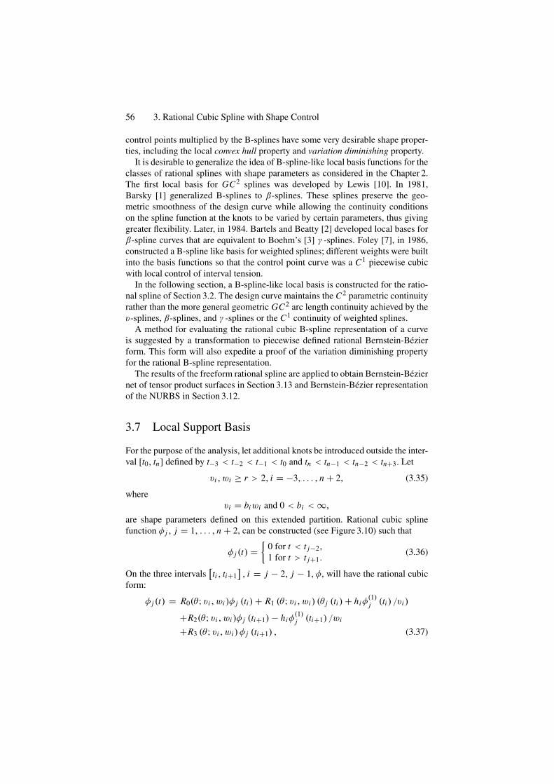
56 3. Rational Cubic Spline with Shape Control
control points multiplied by the B-splines have some very desirable shape proper-ties, including the local convex hull property and variation diminishing property.
It is desirable to generalize the idea of B-spline-like local basis functions for theclasses of rational splines with shape parameters as considered in the Chapter 2.The first local basis for GC2 splines was developed by Lewis [10]. In 1981,Barsky [1] generalized B-splines to β-splines. These splines preserve the geo-metric smoothness of the design curve while allowing the continuity conditionson the spline function at the knots to be varied by certain parameters, thus givinggreater flexibility. Later, in 1984. Bartels and Beatty [2] developed local bases forβ-spline curves that are equivalent to Boehm’s [3] γ -splines. Foley [7], in 1986,constructed a B-spline like basis for weighted splines; different weights were builtinto the basis functions so that the control point curve was a C1 piecewise cubicwith local control of interval tension.
In the following section, a B-spline-like local basis is constructed for the ratio-nal spline of Section 3.2. The design curve maintains the C2 parametric continuityrather than the more general geometric GC2 arc length continuity achieved by thev-splines, β-splines, and γ -splines or the C1 continuity of weighted splines.
A method for evaluating the rational cubic B-spline representation of a curveis suggested by a transformation to piecewise defined rational Bernstein-Bezierform. This form will also expedite a proof of the variation diminishing propertyfor the rational B-spline representation.
The results of the freeform rational spline are applied to obtain Bernstein-Beziernet of tensor product surfaces in Section 3.13 and Bernstein-Bezier representationof the NURBS in Section 3.12.
3.7 Local Support Basis
For the purpose of the analysis, let additional knots be introduced outside the inter-val [t0, tn] defined by t−3 < t−2 < t−1 < t0 and tn < tn−1 < tn−2 < tn+3. Let
vi , wi ≥ r > 2, i = −3, . . . , n + 2, (3.35)
wherevi = biwi and 0 < bi < ∞,
are shape parameters defined on this extended partition. Rational cubic splinefunction φ j , j = 1, . . . , n + 2, can be constructed (see Figure 3.10) such that
φ j (t) ={
0 for t < t j−2,1 for t > t j+1.
(3.36)
On the three intervals[ti , ti+1
], i = j − 2, j − 1, φ, will have the rational cubic
form:
φ j (t) = R0(θ; vi , wi )φ j (ti ) + R1 (θ; vi , wi ) (θ j (ti ) + hiφ(1)j (ti ) /vi )
+R2(θ; vi , wi )φ j (ti+1) − hiφ(1)j (ti+1) /wi
+R3 (θ; vi , wi ) φ j (ti+1) , (3.37)
3.7. Local Support Basis 57
tj − 2 tj − 1 tj + 1tj
FIGURE 3.10. The rational spline φ j (t).
where Rk (θ; vi , wi ) , k = 0, 1, 2, 3 are defined as in Section 3.2, from Equa-tions (3.1) and (3.4). The requirement that φ j ∈ C2(−∞,∞) (in particular, att j−2, t j−1, t j , t j+1) uniquely determines φ j , since it can then be shown that
φ j(t j−2
) = φ(1)j(t j−2
) = 0,
φ j (t j−1) = µ j−1, φ(1)j (t j−1) = µ j−1,
φ j (t j ) = 1 − λ j , φ(1)j t j = λ j ,
⎫⎪⎬
⎪⎭(3.38)
where
λ j = h jλ j/v j , µ j = h j−1µ j/w j−1,
λ j = h j d j−1/c j , µ j = h j−1d j+1/c j+1,
}(3.39)
c j = h j−1d j−1 + h jv j−1d j−1
(h j−1
w j−1+ h j
v j
),
and
d j = h j(w j−1(w j−1 − 1) − v j−1
)/w j−1 + h j−1
(v j (v j − 1) − w j
)/v j .
The local support rational cubic B-spline basis is now defined by the differencefunctions:
B j (t) = ϕ j (t) − ϕ j+1 (t) , j = −1, . . . , n + 1. (3.40)
Thus, there immediately follows:
Proposition 3.15. (Rational B-spline) The rational spline functions B j (t) , j =−1, . . . , n + 1 are such that
(Local support) B j (t) = 0, for t ∈ (t j−2, t j+2), (3.41)
(Partition of unity)
n+1∑
j=−1
B j (t) = 1 for t ∈ [t0, tn] . (3.42)
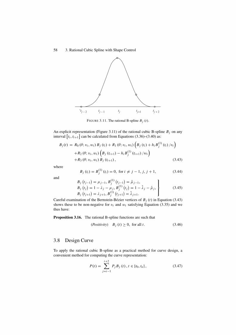
58 3. Rational Cubic Spline with Shape Control
'tj − 2 tj − 1 tj+1 tj + 2tj
FIGURE 3.11. The rational B-spline B j (t).
An explicit representation (Figure 3.11) of the rational cubic B-spline B j on anyinterval
[ti , ti+1
]can be calculated from Equations (3.36)–(3.40) as:
B j (t) = R0 (θ; vi , wi ) B j (ti ) + R1 (θ; vi , wi )(
B j (ti ) + hi B(1)j (ti ) /vi
)
+R2 (θ; vi , wi )(
B j (ti+1) − hi B(1)j (ti+1) /wi
)
+R3 (θ; vi , wi ) B j (ti+1) , (3.43)
whereB j (ti ) = B(1)
j (ti ) = 0, for i = j − 1, j, j + 1, (3.44)
andB j(t j−1
) = µ j−1, B(1)j(t j−1
) = µ j−1,
B j(t j) = 1 − λ j − µ j , B(1)
j(t j) = 1 − λ j − µ j ,
B j(t j+1
) = λ j+1, B(1)j(t j+1
) = λ j+1.
⎫⎪⎬
⎪⎭(3.45)
Careful examination of the Bernstein-Bezier vertices of B j (t) in Equation (3.43)shows these to be non-negative for vi and wi satisfying Equation (3.35) and wethus have:
Proposition 3.16. The rational B-spline functions are such that
(Positivity) B j (t) ≥ 0, for all t. (3.46)
3.8 Design Curve
To apply the rational cubic B-spline as a practical method for curve design, aconvenient method for computing the curve representation:
P(t) =i+2∑
j=i−1
Pj B j (t) , t ∈ [t0, tn] , (3.47)
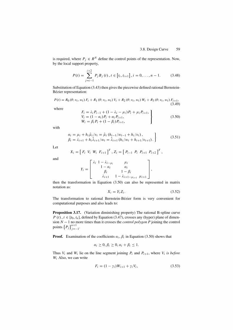
3.8. Design Curve 59
is required, where Pj ∈ RN define the control points of the representation. Now,by the local support property,
P(t) =i+2∑
j=i−1
Pj B j (t) , t ∈ [ti , ti+1], i = 0, . . . , n − 1. (3.48)
Substitution of Equation (3.43) then gives the piecewise defined rational Bernstein-Bezier representation:
P(t) = R0 (θ; vi , wi ) Fi + R1 (θ; vi , wi ) Vi + R2 (θ; vi , wi ) Wi + R3 (θ; vi , wi ) Fi+1,(3.49)
whereFi = λi Pi−1 + (1 − λi − µi )Pi + µi Pi+1,Vi = (1 − αi )Pi + αi Pi+1,Wi = βi Pi + (1 − βi )Pi+1,
⎫⎬
⎭(3.50)
with
αi = µi + hi µi/vi = µi (hi−1/wi−1 + hi/vi ) ,
βi = λi+1 + hi λi+1/wi = λi+1 (hi/wi + hi+1/vi+1) .
}(3.51)
LetXi = [ Fi Vi Wi Fi+1
]T, Zi = [ Pi−1 Pi Pi+1 Pi+2
]T,
and
Yi =
⎡
⎢⎢⎣
λi 1 − λi−µi µi1 − αi αi
βi 1 − βiλi+1 1 − λi+1−µi+1 µi+1
⎤
⎥⎥⎦ ,
then the transformation in Equation (3.50) can also be represented in matrixnotation as:
Xi = Yi Zi . (3.52)
The transformation to rational Bernstein-Bezier form is very convenient forcomputational purposes and also leads to:
Proposition 3.17. (Variation diminishing property) The rational B-spline curveP (t) , t ∈ [t0, tn], defined by Equation (3.47), crosses any (hyper) plane of dimen-sion N − 1 no more times than it crosses the control polygon P joining the controlpoints
{Pj}n+1
j=−1.
Proof. Examination of the coefficients αi , βi in Equation (3.50) shows that
αi ≥ 0, βi ≥ 0, αi + βi ≤ 1.
Thus Vi and Wi lie on the line segment joining Pi and Pi+1, where Vi is beforeWi Also, we can write
Fi = (1 − γi )Wi+1 + γi Vi , (3.53)
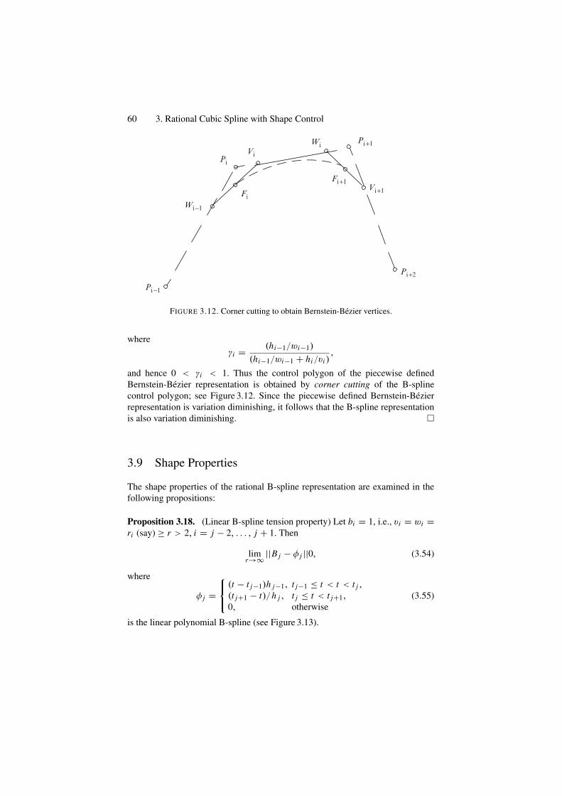
60 3. Rational Cubic Spline with Shape Control
Wi−1
Wi
Pi
Vi
Pi−1
Pi+1
Pi+2
Fi+1
FiVi+1
FIGURE 3.12. Corner cutting to obtain Bernstein-Bezier vertices.
whereγi = (hi−1/wi−1)
(hi−1/wi−1 + hi/vi ),
and hence 0 < γi < 1. Thus the control polygon of the piecewise definedBernstein-Bezier representation is obtained by corner cutting of the B-splinecontrol polygon; see Figure 3.12. Since the piecewise defined Bernstein-Bezierrepresentation is variation diminishing, it follows that the B-spline representationis also variation diminishing. �
3.9 Shape Properties
The shape properties of the rational B-spline representation are examined in thefollowing propositions:
Proposition 3.18. (Linear B-spline tension property) Let bi = 1, i.e., vi = wi =ri (say) ≥ r > 2, i = j − 2, . . . , j + 1. Then
limr→∞ ||B j − φ j ||0, (3.54)
where
φ j =⎧⎨
⎩
(t − t j−1)h j−1, t j−1 ≤ t < t < t j ,(t j+1 − t)/h j , t j ≤ t < t j+1,0, otherwise
(3.55)
is the linear polynomial B-spline (see Figure 3.13).
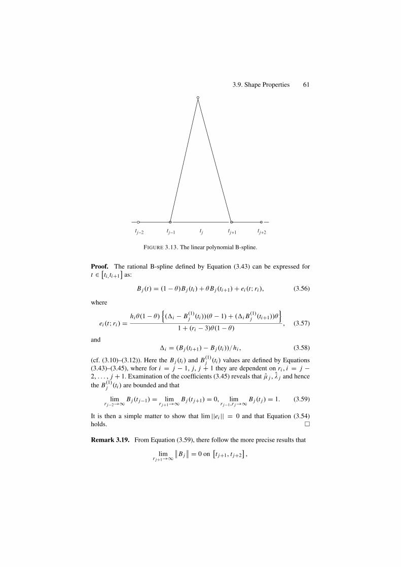
3.9. Shape Properties 61
tj−2 tj−1 tj+1 tj+2tj
FIGURE 3.13. The linear polynomial B-spline.
Proof. The rational B-spline defined by Equation (3.43) can be expressed fort ∈ [ti,ti+1
]as:
B j (t) = (1 − θ)B j (ti ) + θ B j (ti+1) + ei (t; ri ), (3.56)
where
ei (t; ri ) =hiθ(1 − θ)
{(�i − B(1)
j (ti ))(θ − 1) + (�i B(1)j (ti+1))θ
}
1 + (ri − 3)θ(1 − θ), (3.57)
and�i = (B j (ti+1) − B j (ti ))/hi , (3.58)
(cf. (3.10)–(3.12)). Here the B j (ti ) and B(1)j (ti ) values are defined by Equations
(3.43)–(3.45), where for i = j − 1, j, j + 1 they are dependent on ri , i = j −2, . . . , j + 1. Examination of the coefficients (3.45) reveals that µ j , λ j and hencethe B(1)
j (ti ) are bounded and that
limr j−2→∞ B j (t j−1) = lim
r j+1→∞ B j (t j+1) = 0, limr j−1,r j →∞ B j (t j ) = 1. (3.59)
It is then a simple matter to show that lim ||ei || = 0 and that Equation (3.54)holds. �
Remark 3.19. From Equation (3.59), there follow the more precise results that
limr j+1→∞
∥∥B j
∥∥ = 0 on
[t j+1, t j+2
],
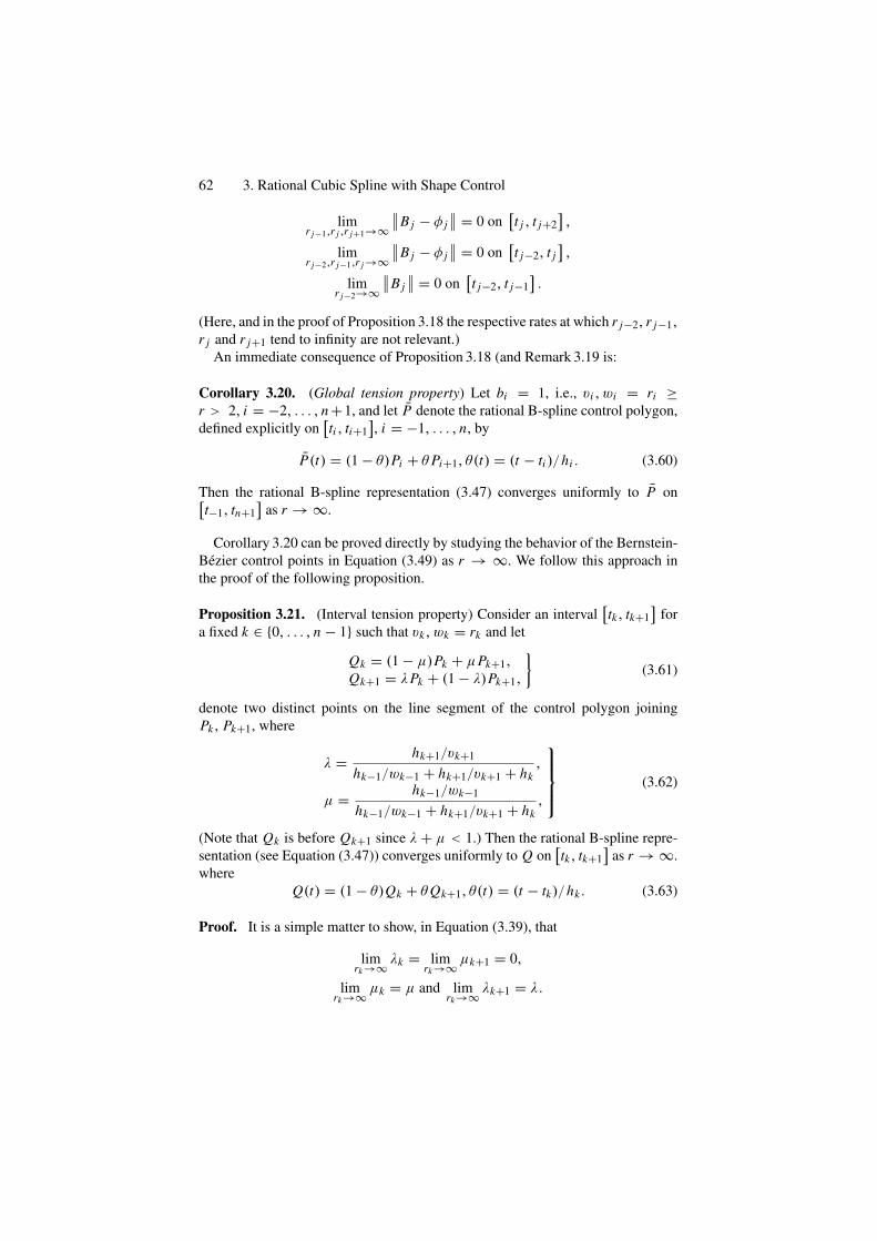
62 3. Rational Cubic Spline with Shape Control
limr j−1,r j ,r j+1→∞
∥∥B j − φ j∥∥ = 0 on
[t j , t j+2
],
limr j−2,r j−1,r j →∞
∥∥B j − φ j
∥∥ = 0 on
[t j−2, t j
],
limr j−2→∞
∥∥B j∥∥ = 0 on
[t j−2, t j−1
].
(Here, and in the proof of Proposition 3.18 the respective rates at which r j−2, r j−1,r j and r j+1 tend to infinity are not relevant.)
An immediate consequence of Proposition 3.18 (and Remark 3.19 is:
Corollary 3.20. (Global tension property) Let bi = 1, i.e., vi , wi = ri ≥r > 2, i = −2, . . . , n +1, and let P denote the rational B-spline control polygon,defined explicitly on
[ti , ti+1
], i = −1, . . . , n, by
P(t) = (1 − θ)Pi + θ Pi+1, θ(t) = (t − ti )/hi . (3.60)
Then the rational B-spline representation (3.47) converges uniformly to P on[t−1, tn+1
]as r → ∞.
Corollary 3.20 can be proved directly by studying the behavior of the Bernstein-Bezier control points in Equation (3.49) as r → ∞. We follow this approach inthe proof of the following proposition.
Proposition 3.21. (Interval tension property) Consider an interval[tk, tk+1
]for
a fixed k ∈ {0, . . . , n − 1} such that vk, wk = rk and let
Qk = (1 − µ)Pk + µPk+1,Qk+1 = λPk + (1 − λ)Pk+1,
}(3.61)
denote two distinct points on the line segment of the control polygon joiningPk, Pk+1, where
λ = hk+1/vk+1
hk−1/wk−1 + hk+1/vk+1 + hk,
µ = hk−1/wk−1
hk−1/wk−1 + hk+1/vk+1 + hk,
⎫⎪⎪⎬
⎪⎪⎭(3.62)
(Note that Qk is before Qk+1 since λ + µ < 1.) Then the rational B-spline repre-sentation (see Equation (3.47)) converges uniformly to Q on
[tk, tk+1
]as r → ∞.
whereQ(t) = (1 − θ)Qk + θ Qk+1, θ(t) = (t − tk)/hk . (3.63)
Proof. It is a simple matter to show, in Equation (3.39), that
limrk→∞ λk = lim
rk→∞ µk+1 = 0,
limrk→∞ µk = µ and lim
rk→∞ λk+1 = λ.
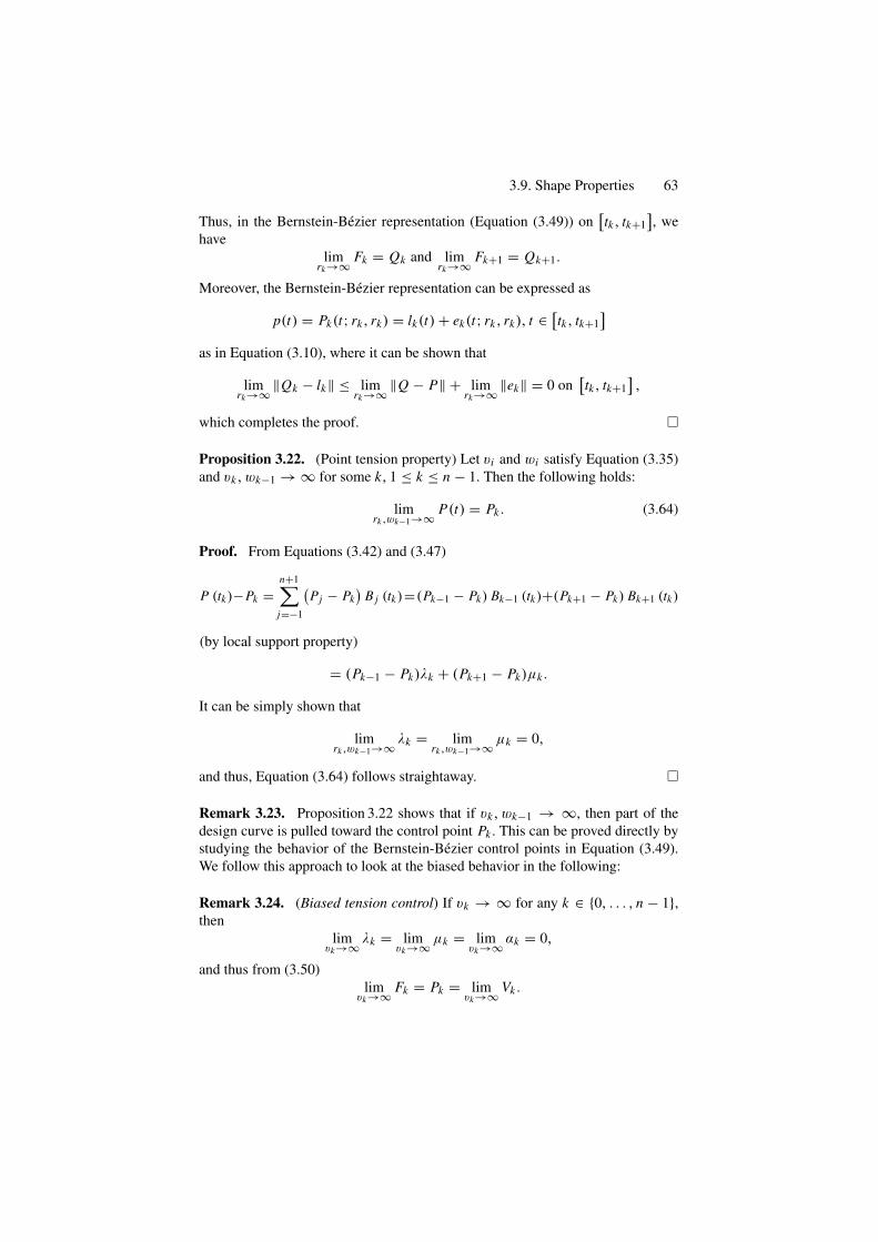
3.9. Shape Properties 63
Thus, in the Bernstein-Bezier representation (Equation (3.49)) on[tk, tk+1
], we
havelim
rk→∞ Fk = Qk and limrk→∞ Fk+1 = Qk+1.
Moreover, the Bernstein-Bezier representation can be expressed as
p(t) = Pk(t; rk, rk) = lk(t) + ek(t; rk, rk), t ∈ [tk, tk+1]
as in Equation (3.10), where it can be shown that
limrk→∞ ‖Qk − lk‖ ≤ lim
rk→∞ ‖Q − P‖ + limrk→∞ ‖ek‖ = 0 on
[tk, tk+1
],
which completes the proof. �
Proposition 3.22. (Point tension property) Let vi and wi satisfy Equation (3.35)and vk, wk−1 → ∞ for some k, 1 ≤ k ≤ n − 1. Then the following holds:
limrk ,wk−1→∞ P(t) = Pk . (3.64)
Proof. From Equations (3.42) and (3.47)
P (tk)−Pk =n+1∑
j=−1
(Pj − Pk
)B j (tk)=(Pk−1 − Pk) Bk−1 (tk)+(Pk+1 − Pk) Bk+1 (tk)
(by local support property)
= (Pk−1 − Pk)λk + (Pk+1 − Pk)µk .
It can be simply shown that
limrk ,wk−1→∞ λk = lim
rk ,wk−1→∞ µk = 0,
and thus, Equation (3.64) follows straightaway. �
Remark 3.23. Proposition 3.22 shows that if vk, wk−1 → ∞, then part of thedesign curve is pulled toward the control point Pk . This can be proved directly bystudying the behavior of the Bernstein-Bezier control points in Equation (3.49).We follow this approach to look at the biased behavior in the following:
Remark 3.24. (Biased tension control) If vk → ∞ for any k ∈ {0, . . . , n − 1},then
limvk→∞ λk = lim
vk→∞ µk = limvk→∞ αk = 0,
and thus from (3.50)lim
vk→∞ Fk = Pk = limvk→∞ Vk .
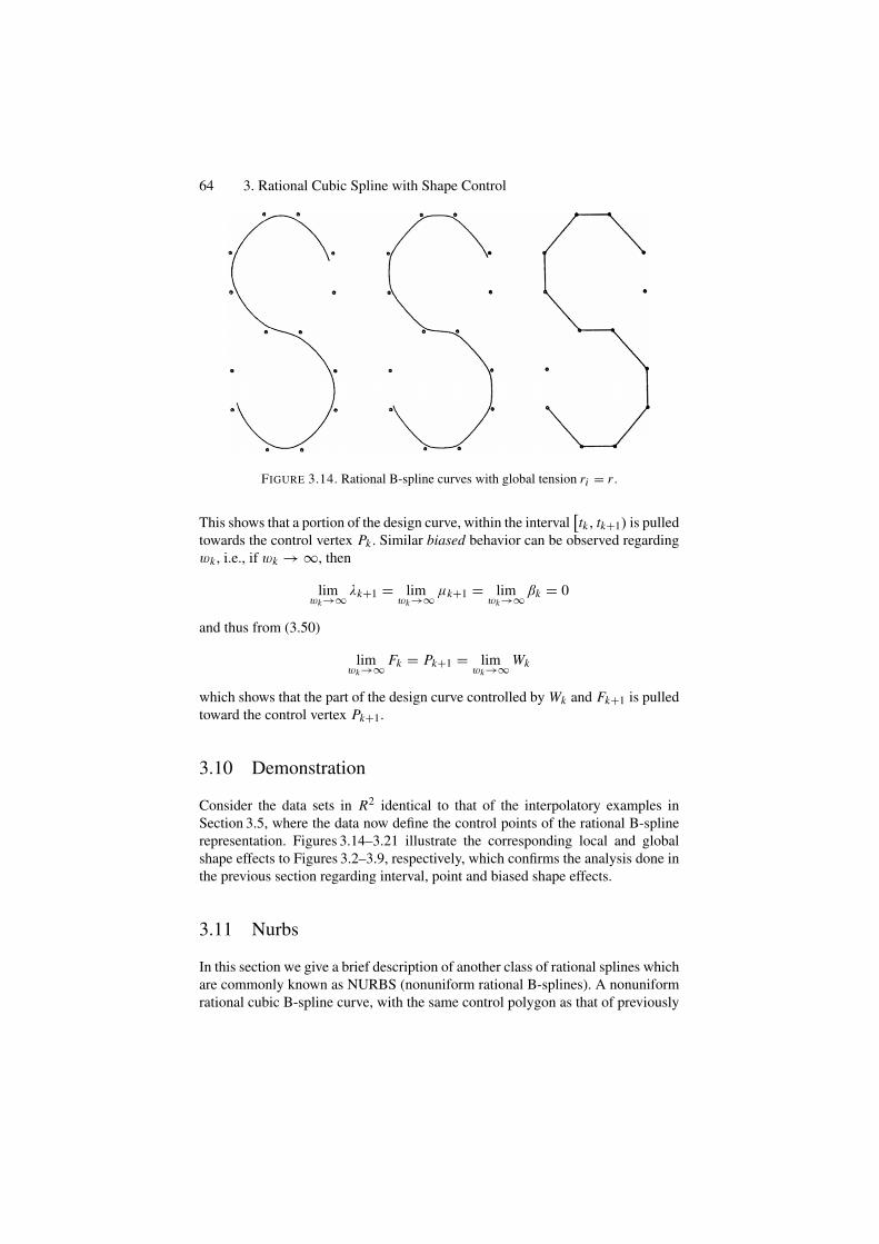
64 3. Rational Cubic Spline with Shape Control
FIGURE 3.14. Rational B-spline curves with global tension ri = r .
This shows that a portion of the design curve, within the interval[tk, tk+1) is pulled
towards the control vertex Pk . Similar biased behavior can be observed regardingwk , i.e., if wk → ∞, then
limwk→∞ λk+1 = lim
wk→∞ µk+1 = limwk→∞ βk = 0
and thus from (3.50)
limwk→∞ Fk = Pk+1 = lim
wk→∞ Wk
which shows that the part of the design curve controlled by Wk and Fk+1 is pulledtoward the control vertex Pk+1.
3.10 Demonstration
Consider the data sets in R2 identical to that of the interpolatory examples inSection 3.5, where the data now define the control points of the rational B-splinerepresentation. Figures 3.14–3.21 illustrate the corresponding local and globalshape effects to Figures 3.2–3.9, respectively, which confirms the analysis done inthe previous section regarding interval, point and biased shape effects.
3.11 Nurbs
In this section we give a brief description of another class of rational splines whichare commonly known as NURBS (nonuniform rational B-splines). A nonuniformrational cubic B-spline curve, with the same control polygon as that of previously
3.11. Nurbs 65
FIGURE 3.15. Rational B-spline curves with tension r4 varying.
FIGURE 3.16. Freeform rational splines can produce looser curves than cubic B-spline.
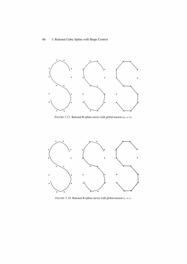
66 3. Rational Cubic Spline with Shape Control
FIGURE 3.17. Rational B-spline curves with global tension wi = w.
FIGURE 3.18. Rational B-spline curves with global tension vi = v .
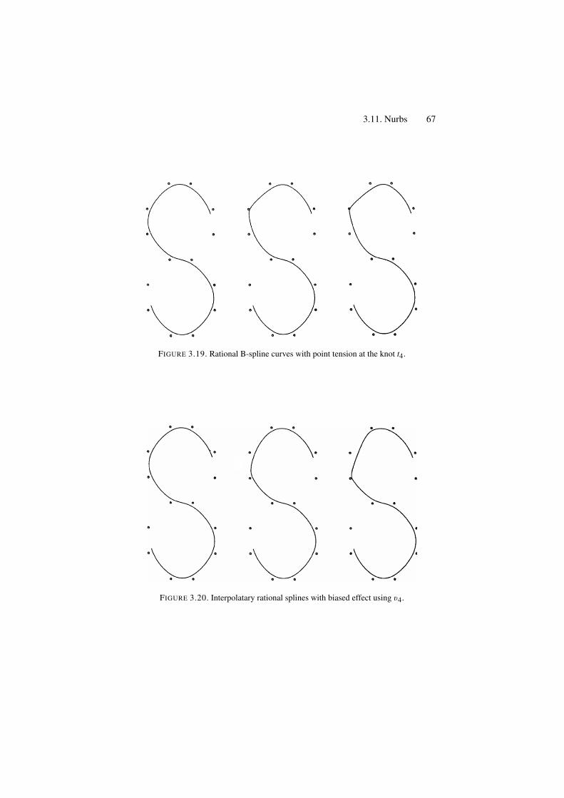
3.11. Nurbs 67
FIGURE 3.19. Rational B-spline curves with point tension at the knot t4.
FIGURE 3.20. Interpolatary rational splines with biased effect using v4.
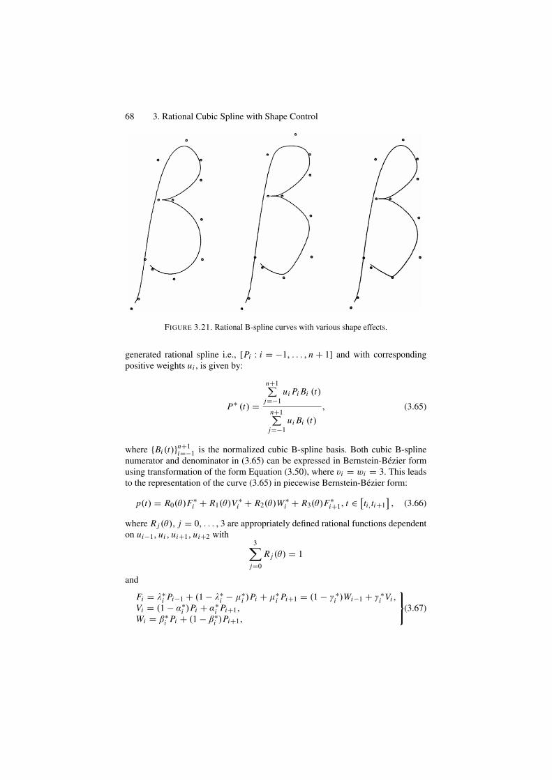
68 3. Rational Cubic Spline with Shape Control
FIGURE 3.21. Rational B-spline curves with various shape effects.
generated rational spline i.e., [Pi : i = −1, . . . , n + 1] and with correspondingpositive weights ui , is given by:
P∗ (t) =
n+1∑
j=−1ui Pi Bi (t)
n+1∑
j=−1ui Bi (t)
, (3.65)
where {Bi (t)}n+1i=−1 is the normalized cubic B-spline basis. Both cubic B-spline
numerator and denominator in (3.65) can be expressed in Bernstein-Bezier formusing transformation of the form Equation (3.50), where vi = wi = 3. This leadsto the representation of the curve (3.65) in piecewise Bernstein-Bezier form:
p(t) = R0(θ)F∗i + R1(θ)V ∗
i + R2(θ)W ∗i + R3(θ)F∗
i+1, t ∈ [ti,ti+1], (3.66)
where R j (θ), j = 0, . . . , 3 are appropriately defined rational functions dependenton ui−1, ui , ui+1, ui+2 with
3∑
j=0
R j (θ) = 1
and
Fi = λ∗i Pi−1 + (1 − λ∗
i − µ∗i )Pi + µ∗
i Pi+1 = (1 − γ ∗i )Wi−1 + γ ∗
i Vi ,Vi = (1 − α∗
i )Pi + α∗i Pi+1,
Wi = β∗i Pi + (1 − β∗
i )Pi+1,
⎫⎬
⎭(3.67)
3.11. Nurbs 69
α∗i = αi ui+1[
(1 − αi )ui + αi ui+1] ,
β∗i = (1 − βi )ui+1[
(1 − βi )ui + βi ui+1] ,
⎫⎪⎪⎪⎬
⎪⎪⎪⎭
(3.68)
γ ∗i = hi−1
[(1 − αi )ui + αi ui+1
]
hi−1[(1 − αi )ui + αi ui+1
]+ hi[1 − βi−1)ui−1 + βi−1ui
] , (3.69)
λ∗i = λi ui−1
λi ui−1(1 − λi − µi )µi + µi ui+1,
µ∗i = µi ui+1
λi ui−1(1 − λi − µi )ui + µi ui+1,
⎫⎪⎪⎪⎬
⎪⎪⎪⎭
(3.70)
αi = hi−1
hi−1 + hi + hi+1,
βi = hi−1 + hi
hi−1 + hi + hi+1,
⎫⎪⎪⎬
⎪⎪⎭(3.71)
λi = h2i
(hi−1 + hi )(hi−2 + hi−1 + hi ),
µi = h2i−1
(hi−1 + hi )(hi−1 + hi + hi+1).
⎫⎪⎪⎪⎬
⎪⎪⎪⎭
(3.72)
Similarly to Equation (3.52), the transformation (in Equation (3.67)) can be repre-sented in matrix notation as:
X∗i = Y ∗
i Z∗i , (3.73)
provided ∗’s are put appropriately. Examination of the coefficients in Equations(3.68)–(3.72) shows that
0 ≤ α∗i , β∗
i , γ ∗i , α∗
i + β∗i ≤ 1. (3.74)
Thus, as in the previously generated rational spline, the control polygon ofthe piecewise defined Bernstein-Bezier representation (Equation (3.66)) can beobtained by corner cutting (see Figure 3.12 with the replacement of the Bernstein-Bezier points by the same points with ∗) of the NURBS control polygon and theNURBS representation is variation diminishing.
Remark 3.25. It can be observed from the algebra of NURBS that if ui → ∞then F∗
i → Pi (for a fixed i) and the design curves sharply toward Pi in theregion of Pi−2 Pi−1 Pi Pi+1 Pi+2. Thus it seems reasonable to assign high weightsin regions where the curve is expected to curve sharply. But, as compared to therational spline (of previous sections), there is not that much freedom for assigningthe weights if all of them are very high. This will not have a significant effecton the curve since a common factor in all weights will simply cancel out. For
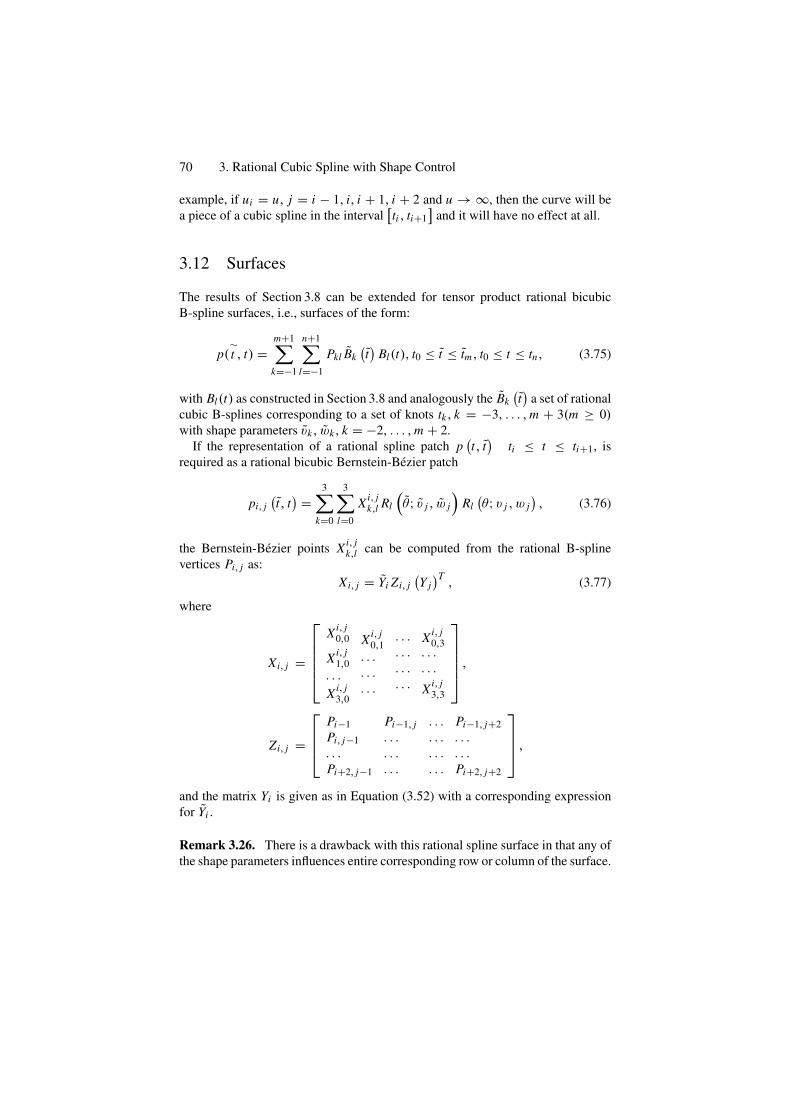
70 3. Rational Cubic Spline with Shape Control
example, if ui = u, j = i − 1, i, i + 1, i + 2 and u → ∞, then the curve will bea piece of a cubic spline in the interval
[ti , ti+1
]and it will have no effect at all.
3.12 Surfaces
The results of Section 3.8 can be extended for tensor product rational bicubicB-spline surfaces, i.e., surfaces of the form:
p(∼t , t) =
m+1∑
k=−1
n+1∑
l=−1
Pkl Bk(t)
Bl(t), t0 ≤ t ≤ tm, t0 ≤ t ≤ tn, (3.75)
with Bl(t) as constructed in Section 3.8 and analogously the Bk(t)
a set of rationalcubic B-splines corresponding to a set of knots tk, k = −3, . . . , m + 3(m ≥ 0)with shape parameters vk, wk, k = −2, . . . , m + 2.
If the representation of a rational spline patch p(t, t)
ti ≤ t ≤ ti+1, isrequired as a rational bicubic Bernstein-Bezier patch
pi, j(t, t) =
3∑
k=0
3∑
l=0
Xi, jk,l Rl
(θ; v j , w j
)Rl(θ; v j , w j
), (3.76)
the Bernstein-Bezier points Xi, jk,l can be computed from the rational B-spline
vertices Pi, j as:Xi, j = Yi Zi, j
(Y j)T
, (3.77)
where
Xi, j =
⎡
⎢⎢⎢⎢⎣
Xi, j0,0
Xi, j1,0
. . .
Xi, j3,0
Xi, j0,1
. . .
. . .
. . .
. . .
. . .
. . .
. . .
Xi, j0,3
· · ·· · ·Xi, j
3,3
⎤
⎥⎥⎥⎥⎦
,
Zi, j =
⎡
⎢⎢⎣
Pi−1Pi, j−1. . .Pi+2, j−1
Pi−1, j. . .. . .. . .
. . .
. . .
. . .
. . .
Pi−1, j+2. . .. . .Pi+2, j+2
⎤
⎥⎥⎦ ,
and the matrix Yi is given as in Equation (3.52) with a corresponding expressionfor Yi .
Remark 3.26. There is a drawback with this rational spline surface in that any ofthe shape parameters influences entire corresponding row or column of the surface.
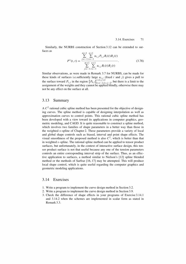
3.14. Exercises 71
Similarly, the NURBS construction of Section 3.12 can be extended to sur-faces as
P∗(t, t) =
m+1∑
j=−1
n+1∑
i=−1ui, j Pi, j Bi (t)B j (t)
m+1∑
j=−1
n+1∑
i=−1ui, j Bi (t)B j (t)
. (3.78)
Similar observations, as were made in Remark 3.7 for NURBS, can be made forthese kinds of surfaces i.e.sufficiently large ui, j (fixed i and j) gives a pull tothe surface toward Pi, j in the region
{Pk,l}i+2, j+2
k=i−2,l= j−2, but there is a limit to theassignment of the weights and they cannot be applied blindly, otherwise there maynot be any effect on the surface at all.
3.13 Summary
A C2 rational cubic spline method has been presented for the objective of design-ing curves. The spline method is capable of designing interpolation as well asapproximation curves to control points. This rational cubic spline method hasbeen developed with a view toward its applications in computer graphics, geo-metric modeling, and CAGD. It is quite reasonable to construct a spline method,which involves two families of shape parameters in a better way than those inthe weighted v-spline of Chapter 2. These parameters provide a variety of localand global shape controls such as biased, interval and point shape effects. Thevisual smoothness of the proposed method is also C2, which is better than thatin weighted v-spline. The rational spline method can be applied to tensor productsurfaces, but unfortunately, in the context of interactive surface design, this ten-sor product surface is not that useful because any one of the tension parameterscontrols an entire corresponding interval strip of the surface. Thus, as an effec-tive application to surfaces, a method similar to Nielson’s [12] spline blendedmethod or the methods of Sarfraz [16, 17] may be attempted. This will producelocal shape control, which is quite useful regarding the computer graphics andgeometric modeling applications.
3.14 Exercises
1. Write a program to implement the curve design method in Section 3.2.2. Write a program to implement the curve design method in Section 3.9.3. Check the difference of shape effects in your programs of Exercise 3.14.1
and 3.14.2 when the schemes are implemented in scalar form as stated inRemark 3.3.

72 3. Rational Cubic Spline with Shape Control
References1. Barsky, B.A. (1981), The Beta-Spline: A Local Representation Based on Shape Para-
meters and Fundamental Geometric Measure, Ph.D. Thesis, University of Utah.2. Bartels, R., and Beatty, J. (1984), Beta-splines with a difference, Technical Report
CS-83-40, Computer Science Department, University of Waterloo, Waterloo, Canada.3. Boehm, W. (1985), Curvature continuous curves and surfaces, Comp Aided Geom
Design 2(2), 313–323.4. Cline, A. (1974), Curve fitting in one dimension using splines under tension, Comm
ACM 17, 218–2235. Dierckx, P., and Tytgat, B. (1989), Generating the Bezier points of β-spline curve,
Comp Aided Geom Design 6, 279–291.6. Farin, G.E. (1996), Curves and Surfaces for CAGD, Academic Press, New York.7. Foley, T.A. (1986), Local control of interval tension using weighted splines. Comp
Aided Geom Design 3, 281–294.8. Foley, T.A. (1987), Interpolation with interval and point tension controls using cubic
weighted Nu-splines, ACM Trans Math Software 13, 68–96.9. Goodman, T.N.T., and Unsworth, K. (1985), Generation of Beta-spline curves
using a recursive relation. In: Fundamental Algorithms for Computer Graphics.R.E. Earnshaw (Ed.), Springer-Verlag, Berlin, pp. 326–357.
10. Lewis, J. (1975), “B-spline” bases for splines under tension, Nu-splines, and frac-tional order splines, Presented at the SIAM-SIGNUM Meeting, San Francisco, CA.
11. Nielson, G.M. (1974), Some piecewise polynomial alternatives to splines under ten-sion, In: Computer-Aided Geometric Design, R.F. Barnhill (Ed.), Academic Press.New York.
12. Nielson, G.M. (1986), Rectangular v-splines. IEEE Comp Graph Appl 6, 35–40.13. Pruess, S. (1979), Alternatives to the exponential spline in tension, Math Comp 33,
1273–1281.14. Salkauskas, K. (1984), C1 splines for interpolation of rapidly varying data, Rocky Mtn.
J. Math 14, 239–250.15. Sarfraz, M. (1992), A C2 rational cubic spline alternative to the NURBS, Comp. &
Graph 16(l), 69–78.16. Sarfraz, M. (1995), Curves and surfaces for CAD using C2 rational cubic splines, Int
J Eng Comput, Springer-Verlag, 11(2), 94–102.17. Sarfraz, M. (1994), Freeform rational bicubic spline surfaces with tension control,
Facta Universitatis (NIS), Ser Math Informatics, 9, 83–93.18. Sarfraz, M. (1994), Cubic spline curves with shape control, Int J Comput & Graphics,
Elsevier Science, 18(5), 707–713.19. Sarfraz, M, (2003), Weighted Nu-splines: an alternative to NURBS, Advances in Geo-
metric Modeling, Ed.: M. Sarfraz, John Wiley, New York, 81–95.20. Schoenburg, I. J. (1946), Contributions to the problem of approximation of equidistant
data by analytic functions, Appl Math 4, 45–99.21. Schweikert, D.G. (1966), An interpolation curve using a spline in tension, J Math Phys
45, 312–317.22. Sarfraz, M. (2004), Weighted Nu-splines with local support basis functions, Int J Com-
put & Graphics, Elsevier Science, 28(4), 539–549.23. Gregory, J.A., and Sarfraz, M. (1990), A rational spline with tension, Int J Comput
Aided Geom Des, North-Holland, Elsevier, 7, 1–13.

References 73
24. Schweikert, D. (1966), An interpolation curve using splines in tension, J Math Phys45, 312–317.
25. Cline, A. (1974), Curve fitting in one dimension using splines under tension, CommACM 17, 218–223.
26. Preuss, S. (1979), Alternatives to the exponential spline in tension, Math Comp 33,1273–1281
27. Boehm, W. (1987), Rational geometric splines, Comput Aided Geom Des 4, 67–77.28. Schoenberg, L. (1981), Spline Functions: Basic Theory, John Wiley, New York.
4Rational Sigma (σ ) Splines
Abstract. As interactive curve design is a basic need for CAD/CAM, computer graphics,vision, imaging and various other disciplines. It is desired to have a robust, visuallypleasant, well-controlled, and effective scheme that can provide a useful solution to manyproblems of different kinds at one platform. A rational spline, with some additional shapeparameters in its description as well as in the description of its piecewise stitching, maybe a good choice in this regard. This chapter has been devoted to a more general rationalspline, known as the sigma (σ ) spline. Although, a σ – spline is a GC1 rational splineas far as its theoretical smoothness is concerned, in most practical cases, it provides aC1, GC2 or C2 solution. It is the most generalized spline in the literature and recovers,as a special case, most of the existing methods in the literature. These methods includeweighted spline, ν – spline, weighted Nu-spline, γ – spline, and so on.
4.1 Introduction
This chapter discusses the rational splines of Chapters 2 and 3 and presents ageneralized description of rational cubics with σ -continuity (c.f. 1.6). The mostgeneral description of rational cubics and σ -continuity constraints provides a vari-ety of shape control parameters which can be sufficient and highly useful for anykind of shape influence such as interval tension, point tension, local tension, globaltension, or biased tensions. Interpolatory and freeform structures of the rationalσ -splines can manage to recover a large number of well-known useful methods[1–28] including weighted splines, ν-splines, weighted ν-splines, gamma-splines,beta-splines, rational β-splines, rational splines of Chapter 2 and 3, and the ratio-nal geometric splines of Boehm.
The approaches adopted in the construction of rational σ -splines are quite anal-ogous to those in Chapters 2 and 3. Section 4.2 discusses the most general formof a rational cubic. The interpolatory and the freeform descriptions of rationalσ -splines are made in Section 4.3 and 4.4, respectively. Some special cases andexamples are discussed at the end of both of theses sections.
75
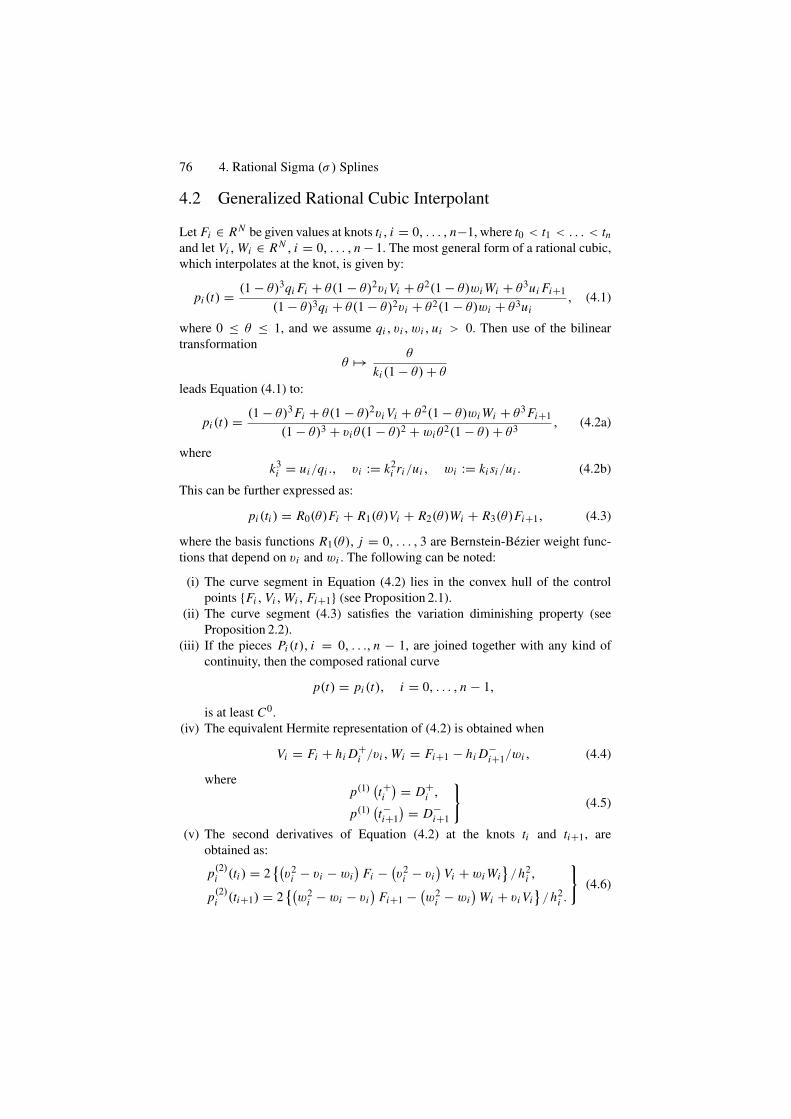
76 4. Rational Sigma (σ ) Splines
4.2 Generalized Rational Cubic Interpolant
Let Fi ∈ RN be given values at knots ti , i = 0, . . . , n−1, where t0 < t1 < . . . < tnand let Vi , Wi ∈ RN , i = 0, . . . , n − 1. The most general form of a rational cubic,which interpolates at the knot, is given by:
pi (t) = (1 − θ)3qi Fi + θ(1 − θ)2vi Vi + θ2(1 − θ)wi Wi + θ3ui Fi+1
(1 − θ)3qi + θ(1 − θ)2vi + θ2(1 − θ)wi + θ3ui, (4.1)
where 0 ≤ θ ≤ 1, and we assume qi , vi , wi , ui > 0. Then use of the bilineartransformation
θ �→ θ
ki (1 − θ) + θ
leads Equation (4.1) to:
pi (t) = (1 − θ)3 Fi + θ(1 − θ)2vi Vi + θ2(1 − θ)wi Wi + θ3 Fi+1
(1 − θ)3 + viθ(1 − θ)2 + wiθ2(1 − θ) + θ3 , (4.2a)
wherek3
i = ui/qi ., vi := k2i ri/ui , wi := ki si/ui . (4.2b)
This can be further expressed as:
pi (ti ) = R0(θ)Fi + R1(θ)Vi + R2(θ)Wi + R3(θ)Fi+1, (4.3)
where the basis functions R1(θ), j = 0, . . . , 3 are Bernstein-Bezier weight func-tions that depend on vi and wi . The following can be noted:
(i) The curve segment in Equation (4.2) lies in the convex hull of the controlpoints {Fi , Vi , Wi , Fi+1} (see Proposition 2.1).
(ii) The curve segment (4.3) satisfies the variation diminishing property (seeProposition 2.2).
(iii) If the pieces Pi (t), i = 0, . . ., n − 1, are joined together with any kind ofcontinuity, then the composed rational curve
p(t) = pi (t), i = 0, . . . , n − 1,
is at least C0.(iv) The equivalent Hermite representation of (4.2) is obtained when
Vi = Fi + hi D+i /vi , Wi = Fi+1 − hi D−
i+1/wi , (4.4)
wherep(1)
(t+i) = D+
i ,
p(1)(t−i+1) = D−
i+1
}
(4.5)
(v) The second derivatives of Equation (4.2) at the knots ti and ti+1, areobtained as:
p(2)i (ti ) = 2
{(v2
i − vi − wi)
Fi − (v2i − vi
)Vi + wi Wi
}/h2
i ,
p(2)i (ti+1) = 2
{(w2
i − wi − vi)
Fi+1 − (w2i − wi
)Wi + vi Vi
}/h2
i .
}
(4.6)
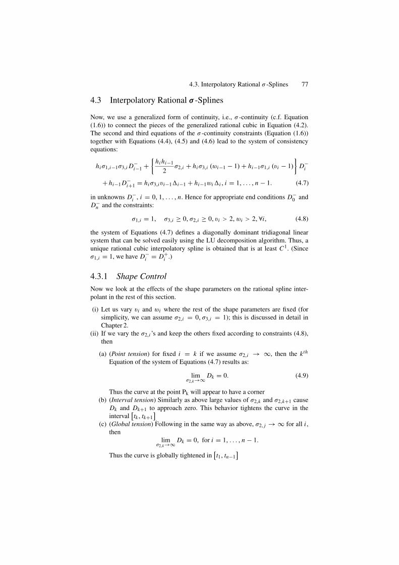
4.3. Interpolatory Rational σ -Splines 77
4.3 Interpolatory Rational σ -Splines
Now, we use a generalized form of continuity, i.e., σ -continuity (c.f. Equation(1.6)) to connect the pieces of the generalized rational cubic in Equation (4.2).The second and third equations of the σ -continuity constraints (Equation (1.6))together with Equations (4.4), (4.5) and (4.6) lead to the system of consistencyequations:
hiσ1,i−1σ3,i D−i−1 +
{hi hi−1
2σ2,i + hiσ3,i (wi−1 − 1) + hi−1σ1,i (vi − 1)
}D−
i
+ hi−1 D−i+1 = hiσ3,ivi−1�i−1 + hi−1wi�i , i = 1, . . . , n − 1. (4.7)
in unknowns D−i , i = 0, 1, . . . , n. Hence for appropriate end conditions D−
0 andD−
n and the constraints:
σ1,i = 1, σ3,i ≥ 0, σ2,i ≥ 0, vi > 2, wi > 2,∀i, (4.8)
the system of Equations (4.7) defines a diagonally dominant tridiagonal linearsystem that can be solved easily using the LU decomposition algorithm. Thus, aunique rational cubic interpolatory spline is obtained that is at least C1. (Sinceσ1,i = 1, we have D−
i = D+i .)
4.3.1 Shape ControlNow we look at the effects of the shape parameters on the rational spline inter-polant in the rest of this section.
(i) Let us vary vi and wi where the rest of the shape parameters are fixed (forsimplicity, we can assume σ2,i = 0, σ3,i = 1); this is discussed in detail inChapter 2.
(ii) If we vary the σ2,i ’s and keep the others fixed according to constraints (4.8),then
(a) (Point tension) for fixed i = k if we assume σ2,i → ∞, then the kth
Equation of the system of Equations (4.7) results as:
limσ2,k→∞ Dk = 0. (4.9)
Thus the curve at the point Pk will appear to have a corner(b) (Interval tension) Similarly as above large values of σ2,k and σ2,k+1 cause
Dk and Dk+1 to approach zero. This behavior tightens the curve in theinterval
[tk, tk+1
].
(c) (Global tension) Following in the same way as above, σ2, j → ∞ for all i ,then
limσ2,k→∞ Dk = 0, for i = 1, . . . , n − 1.
Thus the curve is globally tightened in[t1, tn−1
]
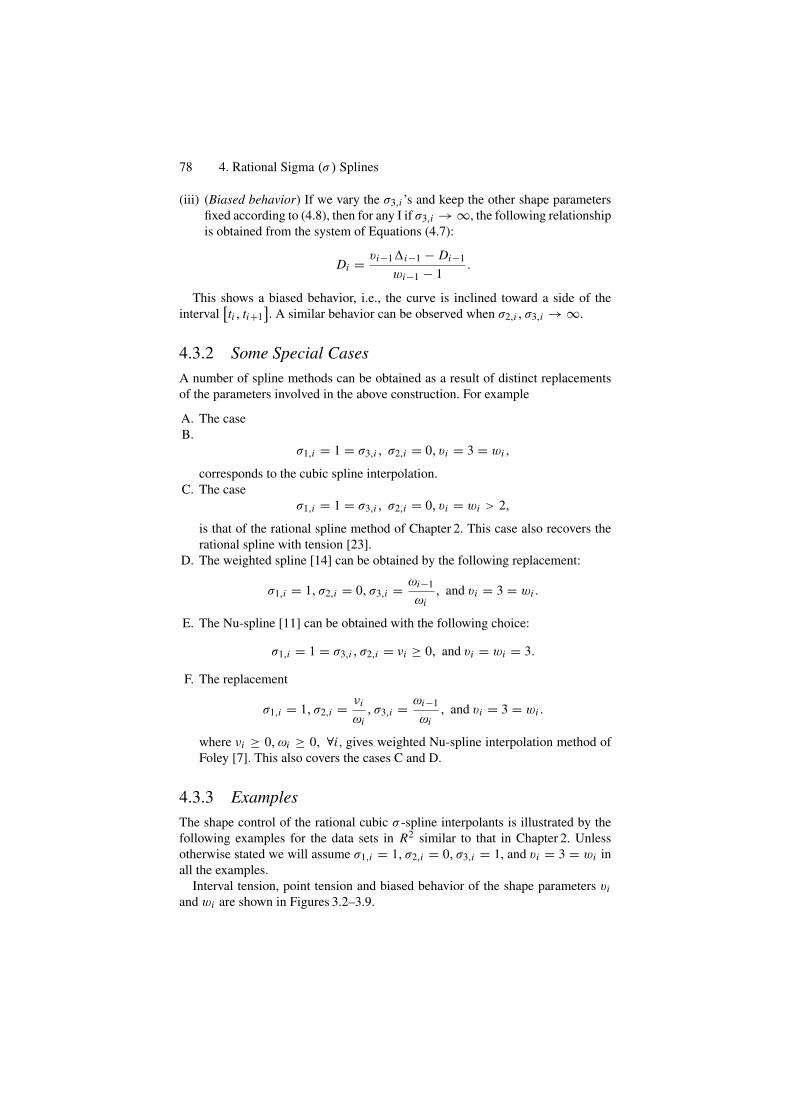
78 4. Rational Sigma (σ ) Splines
(iii) (Biased behavior) If we vary the σ3,i ’s and keep the other shape parametersfixed according to (4.8), then for any I if σ3,i → ∞, the following relationshipis obtained from the system of Equations (4.7):
Di = vi−1�i−1 − Di−1
wi−1 − 1.
This shows a biased behavior, i.e., the curve is inclined toward a side of theinterval
[ti , ti+1
]. A similar behavior can be observed when σ2,i , σ3,i → ∞.
4.3.2 Some Special CasesA number of spline methods can be obtained as a result of distinct replacementsof the parameters involved in the above construction. For example
A. The caseB.
σ1,i = 1 = σ3,i , σ2,i = 0, vi = 3 = wi ,
corresponds to the cubic spline interpolation.C. The case
σ1,i = 1 = σ3,i , σ2,i = 0, vi = wi > 2,
is that of the rational spline method of Chapter 2. This case also recovers therational spline with tension [23].
D. The weighted spline [14] can be obtained by the following replacement:
σ1,i = 1, σ2,i = 0, σ3,i = ωi−1
ωi, and vi = 3 = wi .
E. The Nu-spline [11] can be obtained with the following choice:
σ1,i = 1 = σ3,i , σ2,i = νi ≥ 0, and vi = wi = 3.
F. The replacement
σ1,i = 1, σ2,i = νi
ωi, σ3,i = ωi−1
ωi, and vi = 3 = wi .
where νi ≥ 0, ωi ≥ 0, ∀i , gives weighted Nu-spline interpolation method ofFoley [7]. This also covers the cases C and D.
4.3.3 ExamplesThe shape control of the rational cubic σ -spline interpolants is illustrated by thefollowing examples for the data sets in R2 similar to that in Chapter 2. Unlessotherwise stated we will assume σ1,i = 1, σ2,i = 0, σ3,i = 1, and vi = 3 = wi inall the examples.
Interval tension, point tension and biased behavior of the shape parameters viand wi are shown in Figures 3.2–3.9.
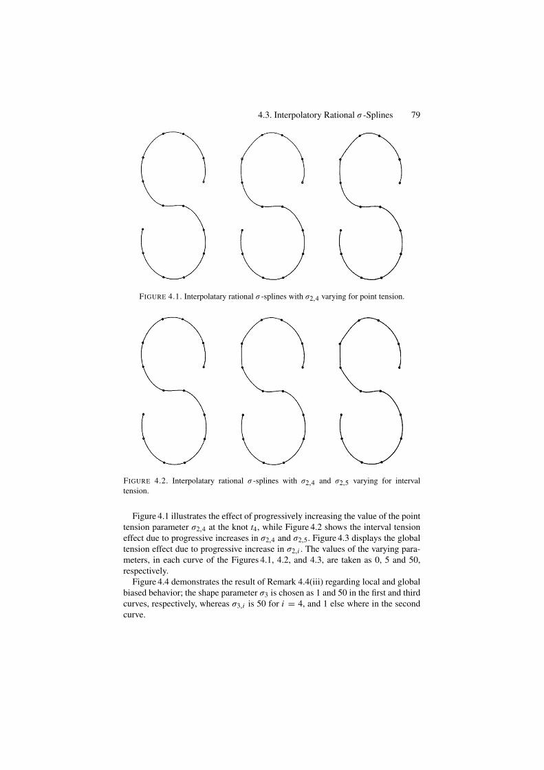
4.3. Interpolatory Rational σ -Splines 79
FIGURE 4.1. Interpolatary rational σ -splines with σ2,4 varying for point tension.
FIGURE 4.2. Interpolatary rational σ -splines with σ2,4 and σ2,5 varying for intervaltension.
Figure 4.1 illustrates the effect of progressively increasing the value of the pointtension parameter σ2,4 at the knot t4, while Figure 4.2 shows the interval tensioneffect due to progressive increases in σ2,4 and σ2,5. Figure 4.3 displays the globaltension effect due to progressive increase in σ2,i . The values of the varying para-meters, in each curve of the Figures 4.1, 4.2, and 4.3, are taken as 0, 5 and 50,respectively.
Figure 4.4 demonstrates the result of Remark 4.4(iii) regarding local and globalbiased behavior; the shape parameter σ3 is chosen as 1 and 50 in the first and thirdcurves, respectively, whereas σ3,i is 50 for i = 4, and 1 else where in the secondcurve.
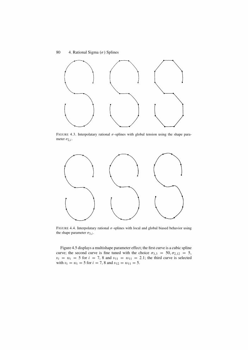
80 4. Rational Sigma (σ ) Splines
FIGURE 4.3. Interpolatary rational σ -splines with global tension using the shape para-meter σ2,i .
FIGURE 4.4. Interpolatary rational σ -splines with local and global biased behavior usingthe shape parameter σ3,i .
Figure 4.5 displays a multishape parameter effect; the first curve is a cubic splinecurve; the second curve is fine tuned with the choice σ3,3 = 50, σ2,12 = 5,vi = wi = 5 for i = 7, 8 and v11 = w11 = 2.1; the third curve is selectedwith vi = wi = 5 for i = 7, 8 and v12 = w11 = 5.
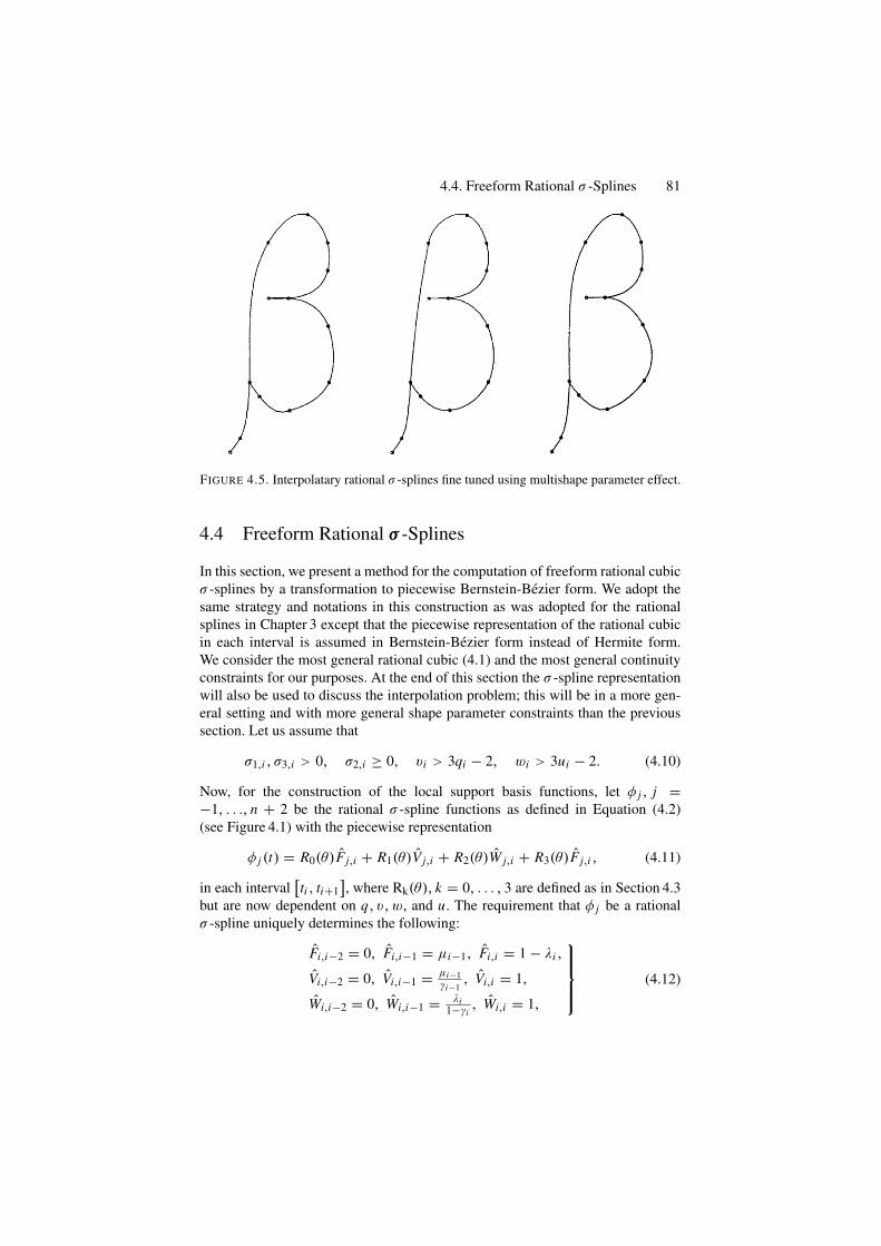
4.4. Freeform Rational σ -Splines 81
FIGURE 4.5. Interpolatary rational σ -splines fine tuned using multishape parameter effect.
4.4 Freeform Rational σ -Splines
In this section, we present a method for the computation of freeform rational cubicσ -splines by a transformation to piecewise Bernstein-Bezier form. We adopt thesame strategy and notations in this construction as was adopted for the rationalsplines in Chapter 3 except that the piecewise representation of the rational cubicin each interval is assumed in Bernstein-Bezier form instead of Hermite form.We consider the most general rational cubic (4.1) and the most general continuityconstraints for our purposes. At the end of this section the σ -spline representationwill also be used to discuss the interpolation problem; this will be in a more gen-eral setting and with more general shape parameter constraints than the previoussection. Let us assume that
σ1,i , σ3,i > 0, σ2,i ≥ 0, vi > 3qi − 2, wi > 3ui − 2. (4.10)
Now, for the construction of the local support basis functions, let φ j , j =−1, . . ., n + 2 be the rational σ -spline functions as defined in Equation (4.2)(see Figure 4.1) with the piecewise representation
φ j (t) = R0(θ)Fj,i + R1(θ)V j,i + R2(θ)W j,i + R3(θ)Fj,i , (4.11)
in each interval[ti , ti+1
], where Rk(θ), k = 0, . . . , 3 are defined as in Section 4.3
but are now dependent on q, v, w, and u. The requirement that φ j be a rationalσ -spline uniquely determines the following:
Fi,i−2 = 0, Fi,i−1 = µi−1, Fi,i = 1 − λi ,
Vi,i−2 = 0, Vi,i−1 = µi−1γi−1
, Vi,i = 1,
Wi,i−2 = 0, Wi,i−1 = λi1−γi
, Wi,i = 1,
⎫⎪⎪⎬
⎪⎪⎭(4.12)
82 4. Rational Sigma (σ ) Splines
where
µi = γiη1,i
ηi,
λi = (1 − λi ) η2,i−1
ηi−1,
γi = hi−1vi ui
hi−1vi ui + hiσ1,i qiwi−1,
⎫⎪⎪⎪⎪⎪⎪⎬
⎪⎪⎪⎪⎪⎪⎭
(4.13a)
η1,i = θ2,i(θ3,i+1 − θ4,i+1
),
η2,i = θ4,i+1(θ1,i − θ2,i
),
ηi = θ1,iθ3,i+1 − θ2,iθ4,i+1,
⎫⎬
⎭(4.13b)
θ1,i = 2h2i−1u2
i−1
{(1 − γi )
(v2
i − vi (3qi − 2))
+ γiwi
}
+ 2hi−2h2i σ2,iγi q2
i wi−1ui−1
+ 2h2i q2
i σ3,i
{γi
(w2
i−1 − wi−1 (3ui−1 − 2) − vi−1
)},
θ2,i = 2h2i−1wi u2
i−1,
θ3,i = 2h2i−1u2
i−1 (1 − γi )(v2
i − vi (3qi − 2) − wi
)
+ 2hi−1h2i σ2,iγi q2
i wi−1ui−1
+ 2h2i q2
i σ3,i
{γi
(w2
i−1 − wi−1 (3ui−1 − 2))
+ (1 − γi ) vi−1
},
θ4,i = 2h2i σ3,i q2
i vi−1.
⎫⎪⎪⎪⎪⎪⎪⎪⎪⎪⎪⎪⎪⎪⎪⎪⎪⎬
⎪⎪⎪⎪⎪⎪⎪⎪⎪⎪⎪⎪⎪⎪⎪⎪⎭
(4.13c)
The local support rational σ -B-spline basis is now defined by the differencefunction B j (t) as in Equation (3.6). Thus if in any interval
[ti , ti+1
],
B j (t) = R0(θ)Fj,i + R1(θ)Vj,i + R2(θ)W j,i + R3(θ)Fj,i , (4.14)
then we have:
Fj,i−2 = 0, i − 1 ≥ j ≥ i + 2, Fi,i−1 = µi−1, Fi,i = 1 − λi − µi , Fi,i+1 = λi+1,
Vj,i−2 = 0, i − 2 ≥ j ≥ i + 1, Vi,i−1 = µi−1
γi−1, Vi,i = 1 − µi
γi,
W j,i−2 = 0, i − 2 ≥ j ≥ i + 1, Wi,i−1 = 1 − λi
1 − γi, Wi,i = λi+1
1 − γi+1.
⎫⎪⎪⎪⎪⎬
⎪⎪⎪⎪⎭
(4.15)
Proposition 4.2. The rational σ -spline functions B j (t), j = −1, . . . , n + l, aresuch that
(Local support) B j (t) = 0 for t ∈ (t j−2, t j+2), (4.16)
(Parti tion of unity)
n+1∑
j=−1
B j (t) = 0 for t ∈ (t j−2, t j+2), (4.17)
(Positively) B j (t) = 0 for all t. (4.18)
4.4. Freeform Rational σ -Splines 83
Proof. The local support and the partition of unity properties follow immediatelyfrom the definition and the construction of the basis functions. For the positivelyproperty (4.18), it can be noted immediately that for the parameters defined in(4.10),
γ j , θi, j > 0, for all j and i = 2, 4. (4.19)
Moreoverθ1, j − θ2, j = θ3, j − θ4, j , (4.20a)
where
θ1, j − θ2, j = 2{
h2j−1u2
j i−1
{(1 − γ j
) (v2
j − v j(3q j − 2
))+ γ jw j
}
+h j−2h2j
2σ2, jγ j q2
j w j−1u j−1
+h2j q
2j σ3, j
{γ j
(w2
j−1 − w j−1(3u j−1 − 2
)) − v j−1
} },(4.20b)
is also positive. Therefore, the quantities η1, j , η2, j and hence
η j = η1, j + η2, j + 2(θ1, j − θ2, j
) (θ3, j+1 − θ4, j+1
), (4.21)
are positive. The above imply that all nonzero terms in Equation (4.15) are positiveand thus Equation (4.18) follows.
To apply the rational cubic B-spline as a practical method for curve design, aconvenient method for computing the curve representation
p(t) =i+2∑
j=i−1
Pj B j (t), t ∈ [t0, tn] , (4.22)
is required, where Pj ∈ RN define the control points of the representation. Now,by the local support property,
p(t) =i+2∑
j=i−1
Pj B j (t), t ∈ [ti , ti+1], i = 0, 1, . . . , n − 1. (4.23)
Substitution of (3.10) then gives the piecewise defined rational Berstein-Bezierrepresentation
p(t) = R0(θ)Fi + R1(θ)Vi + R2(θ)Wi + R3(θ)Fi+1, (4.24)
whereFi = λi Pi−1 + (1 − λi − µi ) Pi + µi Pi+1,Vi = (1 − αi ) Pi + αi Pi+1,Wi = βi Pi + (1 − βi ) Pi+1,
⎫⎬
⎭(4.25)
withαi = η1,i
ηi, βi = η2,i
ηi, (4.26)
84 4. Rational Sigma (σ ) Splines
The transformation to rational Bernstein-Bezier form is very convenient for com-putational purposes and also leads to the following:
Proposition 4.3. (Variation diminishing property) The rational σ -B-spline curvep (t) , t ∈ [t0, tn], defined by Equation (4.22), crosses any (hyper) plane of dimen-sion N −1 no more times than it crosses the control polygon P joining the controlpoints
{Pj}n+1
j=−1.
Proof. Following the arguments in Equations (4.19)–(4.21), for positivity, in theprevious proposition, it is straightforward that the coefficients αi , βi in Equation(4.25) satisfy
αi ≥ 0, βi ≥ 0, αi + βi ≤ 1.
Thus Vi and Wi lie on the line segment joining Pi and Pi+1, where Vi is beforeWi . Also, we write
Fi = (1 − γi ) Wi + γi Vi , (4.27)
where we already know that 0 < γi < 1. Thus the control polygon of the piece-wise defined Bernstein-Bezier representation is obtained by corner cutting of theσ -B-spline control polygon; see Figure 4.3. Since the piecewise defined Bernstein-Bezier representation is variation diminishing, it follows that the σ -B-spline rep-resentation is also variation diminishing.
Remark 4.4. Using the rational σ -B-spline, the interpolation problem of therational σ -splines can be tackled through
n+1∑
j=−1
Pj B j (ti ) = Fi , ∀i. (4.28)
where the matrix of the B j (ti ) is tridiagonal matrix. Since 0 < µi , λi < 1/2,the tridiagonal system of Equations (4.28) is diagonally dominant. Thus a uniqueinterpolatory rational σ -spline exits with more general shape constraints (4.10)than (4.8) in Section 4.3.
4.4.1 Shape ControlThe parameters defined in Equation (4.10) can be used to control the local orglobal shape of the curve:
(i) Since the shape constraints vi > 3qi − 2 and wi > 3ui − 2 must be satisfied,then increase or decrease in qi and ui corresponds to increase or decreasein vi and wi , respectively. Keeping qi and ui fixed (say, qi = ui = 1, forsimplicity) and varying vi and wi is discussed in detail in Chapter 3 wherethe interval, point and the biased behaviors were observed by using theseparameters.
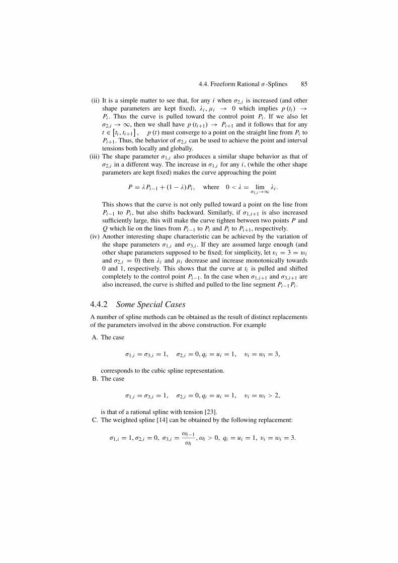
4.4. Freeform Rational σ -Splines 85
(ii) It is a simple matter to see that, for any i when σ2,i is increased (and othershape parameters are kept fixed), λi , µi → 0 which implies p (ti ) →Pi . Thus the curve is pulled toward the control point Pi . If we also letσ2,i → ∞, then we shall have p (ti+1) → Pi+1 and it follows that for anyt ∈ [ti , ti+1
], p (t) must converge to a point on the straight line from Pi to
Pi+1. Thus, the behavior of σ2,i can be used to achieve the point and intervaltensions both locally and globally.
(iii) The shape parameter σ1,i also produces a similar shape behavior as that ofσ2,i in a different way. The increase in σ1,i for any i , (while the other shapeparameters are kept fixed) makes the curve approaching the point
P = λPi−1 + (1 − λ)Pi , where 0 < λ = limσ1,i →∞ λi .
This shows that the curve is not only pulled toward a point on the line fromPi−1 to Pi , but also shifts backward. Similarly, if σ1,i+1 is also increasedsufficiently large, this will make the curve tighten between two points P andQ which lie on the lines from Pi−1 to Pi and Pi to Pi+1, respectively.
(iv) Another interesting shape characteristic can be achieved by the variation ofthe shape parameters σ1,i and σ3,i . If they are assumed large enough (andother shape parameters supposed to be fixed; for simplicity, let vi = 3 = wiand σ2,i = 0) then λi and µi decrease and increase monotonically towards0 and 1, respectively. This shows that the curve at ti is pulled and shiftedcompletely to the control point Pi−1. In the case when σ1,i+1 and σ3,i+1 arealso increased, the curve is shifted and pulled to the line segment Pi−1 Pi .
4.4.2 Some Special CasesA number of spline methods can be obtained as the result of distinct replacementsof the parameters involved in the above construction. For example
A. The case
σ1,i = σ3,i = 1, σ2,i = 0, qi = ui = 1, vi = wi = 3,
corresponds to the cubic spline representation.B. The case
σ1,i = σ3,i = 1, σ2,i = 0, qi = ui = 1, vi = wi > 2,
is that of a rational spline with tension [23].C. The weighted spline [14] can be obtained by the following replacement:
σ1,i = 1, σ2,i = 0, σ3,i = ωi−1
ωi, ωi > 0, qi = ui = 1, vi = wi = 3.
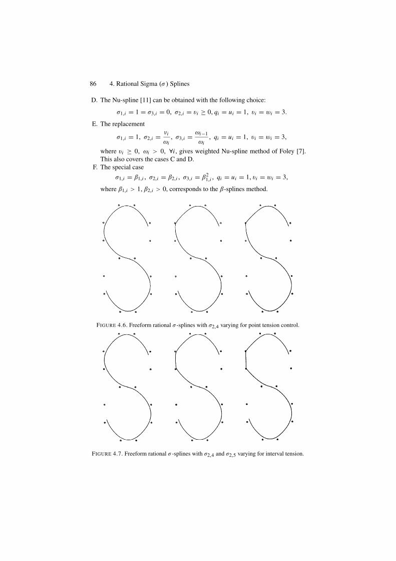
86 4. Rational Sigma (σ ) Splines
D. The Nu-spline [11] can be obtained with the following choice:
σ1,i = 1 = σ3,i = 0, σ2,i = vi ≥ 0, qi = ui = 1, vi = wi = 3.
E. The replacement
σ1,i = 1, σ2,i = νi
ωi, σ3,i = ωi−1
ωi, qi = ui = 1, vi = wi = 3,
where vi ≥ 0, ωi > 0, ∀i , gives weighted Nu-spline method of Foley [7].This also covers the cases C and D.
F. The special caseσ1,i = β1,i , σ2,i = β2,i , σ3,i = β2
1,i , qi = ui = 1, vi = wi = 3,
where β1,i > 1, β2,i > 0, corresponds to the β-splines method.
FIGURE 4.6. Freeform rational σ -splines with σ2,4 varying for point tension control.
FIGURE 4.7. Freeform rational σ -splines with σ2,4 and σ2,5 varying for interval tension.
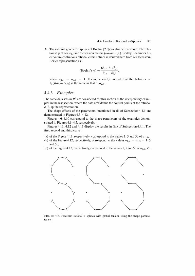
4.4. Freeform Rational σ -Splines 87
G. The rational geometric splines of Boehm [27] can also be recovered. The rela-tionship of our σ2,i and the tension factors (Boehm’s γi ) used by Boehm for hiscurvature continuous rational cubic splines is derived here from our BernsteinBezier representation as:
(Boehm’sγi ) = 6hi−1hi u2i−1
θ1,i − θ2,i,
where σ1,i = σ3,i = 1. It can be easily noticed that the behavior of1/(Boehm’sγi ) is the same as that of σ2,i .
4.4.3 ExamplesThe same data sets in R2 are considered for this section as the interpolatory exam-ples in the last section, where the data now define the control points of the rationalσ -B-spline representation.
The shape effects of the parameters, mentioned in (i) of Subsection 4.4.1 aredemonstrated in Figures 4.5–4.12.
Figures 4.6–4.10 correspond to the shape parameters of the examples demon-strated in Figures 4.1–4.5, respectively.
Figures 4.11, 4.12 and 4.13 display the results in (iii) of Subsection 4.4.1. Thefirst, second and third curve:
(a) of the Figure 4.11, respectively, correspond to the values 1, 5 and 50 of σ1,5,(b) of the Figure 4.12, respectively, correspond to the values σ1,4 = σ1,5 = 1, 5
and 50,(c) of the Figure 4.13, respectively, correspond to the values 1, 5 and 50 of σ1,i ,∀i .
FIGURE 4.8. Freeform rational σ -splines with global tension using the shape parame-ter σ2,i .
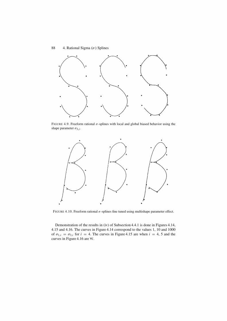
88 4. Rational Sigma (σ ) Splines
FIGURE 4.9. Freeform rational σ -splines with local and global biased behavior using theshape parameter σ3,i .
FIGURE 4.10. Freeform rational σ -splines fine tuned using multishape parameter effect.
Demonstration of the results in (iv) of Subsection 4.4.1 is done in Figures 4.14,4.15 and 4.16. The curves in Figure 4.14 correspond to the values 1, 10 and 1000of σ1,i = σ3,i for i = 4. The curves in Figure 4.15 are when i = 4, 5 and thecurves in Figure 4.16 are ∀i .
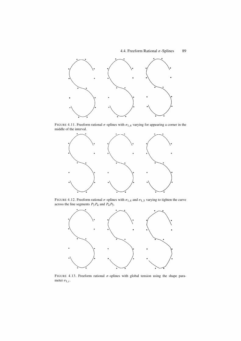
4.4. Freeform Rational σ -Splines 89
FIGURE 4.11. Freeform rational σ -splines with σ1,4 varying for appearing a corner in themiddle of the interval.
FIGURE 4.12. Freeform rational σ -splines with σ1,4 and σ1,5 varying to tighten the curveacross the line segments P3 P4 and P4 P5.
FIGURE 4.13. Freeform rational σ -splines with global tension using the shape para-meter σ1,i .
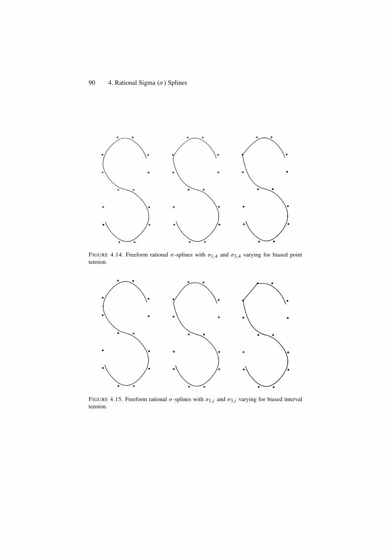
90 4. Rational Sigma (σ ) Splines
FIGURE 4.14. Freeform rational σ -splines with σ1,4 and σ3,4 varying for biased pointtension.
FIGURE 4.15. Freeform rational σ -splines with σ1,i and σ3,i varying for biased intervaltension.
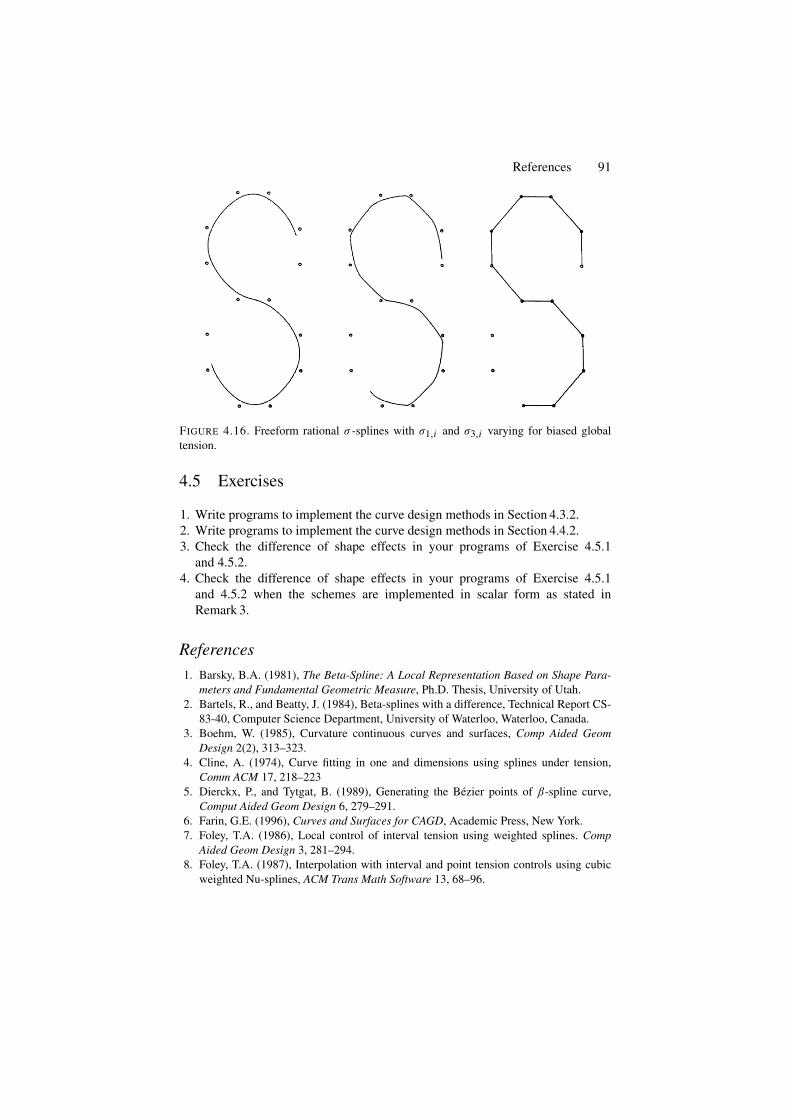
References 91
FIGURE 4.16. Freeform rational σ -splines with σ1,i and σ3,i varying for biased globaltension.
4.5 Exercises
1. Write programs to implement the curve design methods in Section 4.3.2.2. Write programs to implement the curve design methods in Section 4.4.2.3. Check the difference of shape effects in your programs of Exercise 4.5.1
and 4.5.2.4. Check the difference of shape effects in your programs of Exercise 4.5.1
and 4.5.2 when the schemes are implemented in scalar form as stated inRemark 3.
References1. Barsky, B.A. (1981), The Beta-Spline: A Local Representation Based on Shape Para-
meters and Fundamental Geometric Measure, Ph.D. Thesis, University of Utah.2. Bartels, R., and Beatty, J. (1984), Beta-splines with a difference, Technical Report CS-
83-40, Computer Science Department, University of Waterloo, Waterloo, Canada.3. Boehm, W. (1985), Curvature continuous curves and surfaces, Comp Aided Geom
Design 2(2), 313–323.4. Cline, A. (1974), Curve fitting in one and dimensions using splines under tension,
Comm ACM 17, 218–2235. Dierckx, P., and Tytgat, B. (1989), Generating the Bezier points of β-spline curve,
Comput Aided Geom Design 6, 279–291.6. Farin, G.E. (1996), Curves and Surfaces for CAGD, Academic Press, New York.7. Foley, T.A. (1986), Local control of interval tension using weighted splines. Comp
Aided Geom Design 3, 281–294.8. Foley, T.A. (1987), Interpolation with interval and point tension controls using cubic
weighted Nu-splines, ACM Trans Math Software 13, 68–96.

92 4. Rational Sigma (σ ) Splines
9. Goodman, T.N.T., and Unsworth, K. (1985), Generation of beta spline curves using arecursive relation. In: Fundamental Algorithms for Computer Graphics. R.E. Earnshaw(Ed.), Springer-Verlag, Berlin, pp. 326–357.
10. Lewis, J. (1975), “B-spline” bases for splines under tension, Nu-splines, and fractionalorder splines, Presented at the SIAM-SIGNUM Meeting, San Francisco, CA.
11. Nielson, G.M. (1974), Some piecewise polynomial alternatives to splines under ten-sion, In: Computer-Aided Geometric Design, R.F. Barnhill (Ed.), Academic Press.New York.
12. Nielson, G.M. (1986), Rectangular ν-splines. IEEE Comp Graph Appl 6, 35–40.13. Pruess, S. (1979), Alternatives to the exponential spline in tension, Math Comp 33,
1273–1281.14. Salkauskas, K. (1984), C1 splines for interpolation of rapidly varying data, Rocky Mtn
J Math 14, 239–250.15. Sarfraz, M. (1992), A C2 rational cubic spline alternative to the NURBS, Comp &
Graph 16(l), 69–78.16. Sarfraz, M. (1995), Curves and surfaces for CAD using C2 rational cubic splines, Int
J Eng Comput, Springer-Verlag, 11(2), 94–102.17. Sarfraz, M. (1994), Freeform rational bicubic spline surfaces with tension control,
Facta Universitatis (NIS), Ser. Mathematics and Informatics, 9, 83–93.18. Sarfraz, M. (1994), Cubic spline curves with shape control, Int J Comput Graphics,
Elsevier Science, 18(5), 707–713.19. Sarfraz, M, (2003), Weighted Nu-splines: an alternative to NURBS, Advances in Geo-
metric Modeling, Ed.: M. Sarfraz, John Wiley, New York, pp. 81–95.20. Schoenburg, I. J. (1946), Contributions to the problem of approximation of equidistant
data by analytic functions, Appl Math 4, 45–99.21. Schweikert, D.G. (1966), An interpolation curve using a spline in tension, J Math Phys
45, 312–317.22. Sarfraz, M. (2004), Weighted Nu-splines with local support basis functions, Int J Com-
put Graphics, Elsevier Science, 28(4), 539–549.23. Gregory, J.A., and Sarfraz, M. (1990), A rational spline with tension, Int J Comput
Aided Geom Des, North-Holland, Elsevier, 7, 1–13.24. Schweikert, D. (1966), An interpolation curve using splines in tension, J Math and
Phys. 45, 312–317.25. Cline, A. (1974), Curve fitting in one and dimensions using splines under tension,
Comm ACM 17, 218–223.26. Preuss, S. (1979), Alternatives to the exponential spline in tension, Math Comp 33,
1273–128127. Boehm, W. (1987), Rational geometric splines, Comput Aided Geom Des 4, 67–77.28. Schoenberg, L. (1981), Spline Functions: Basic Theory, JohnWiley, New York.
5Linear, Conic and Rational CubicSplines
Abstract. A rational cubic spline has been used with the view to its applications in com-puter graphics, vision, and image processing. It incorporates linear, conic and parametriccubic curve sections as special cases. The parameters (weights), in the description of thespline curve can be used to modify the shape of the curve, locally and globally. The splineattains parametric smoothness of different degrees depending on different choices of deriv-ative settings and nature of curve segments. However, the stitching of the rational cubicsegments preserves C2 smoothness and stitching of the conic segments preserves visuallyreasonable C1 smoothness at the neighboring knots. The curve scheme is interpolatory andcan plot parabolic, hyperbolic, elliptic, and circular splines independently as well as bitsand pieces of a rational cubic spline. This chapter discusses cases of elliptic arcs in spaceand also introduces intermediate point interpolation scheme which can force the curve topass through given point between any segment.
5.1 Introduction
A common problem, in computer graphics, vision, and imaging is to design acurved outline by stitching small pieces of curves together [1–14]. Piecewise ratio-nal cubic spline functions provide powerful tools for designing of curves, sur-faces and some analytic primitives such as conic sections that are widely used inengineering design and various other applications. Such applications may includerepresenting a font outline [13], the round corner of an object [3], or a smoothfit to given data [9]. Several segments of curves, to compose a desired curveoutline, can have different mathematical descriptions. For example, a font “S”when designed, appears to have straight lines, conics, and cubics as essentialparts of its outline. Single mathematical formulation for the precise definition ofvarious types of geometry shapes is one of the major advantages of the rationalcubic spline functions. We aim in this chapter to represent a piecewise parametriccurve scheme, which has all the design features to produce a desired manipu-lated curve.
93

94 5. Linear, Conic and Rational Cubic Splines
In [2], C1 rational cubic splines with exact derivatives for control points wereused. This chapter introduces a similar interpolant but with a very simple distance-based approximated derivative scheme as well as an exact derivative scheme. Ourgoal is to achieve results for problems in various applications. This chapter alsodescribes the parametric C1 and C2 rational cubic spline representation containinga family of shape control parameters. This family of shape parameters has beenused to produce straight-line segments, conics and cubics.
The following features are also a significant addition to the chapter:
• maintaining a reasonable amount of continuity (C1) between conic and cubicarcs,
• estimated end derivatives,• conic (circular, elliptical, parabolic and hyperbolic) splines,• circular arcs for s given radius or center,• elliptic arc in space and• intermediate point interpolation
In [2], the end derivatives are based on the assumption of the user, which isnot convenient. Moreover, the conics are not discussed at all. This chapter hasa description of suitable end derivatives for more pleasing results [14]. In [10],cubic and conic segments are joined with G1 continuity, which is not reasonablefor some practical applications. Intermediate point interpolation scheme and cir-cular arcs, presented in [5], are not practical because the space curves and exactcircular arcs are not possible. In [11], intermediate point interpolation scheme withC0 continuity at neighborhood points was offered. G1 continuity on constrainedguided curve scheme has been introduced in [6] where rational quadratic func-tions were used. This chapter discusses rational cubic function and offers bettercontinuity. In [4], the rational quadratic spline is used for the circular spline. Thischapter uses a very simple technique [10] using a rational cubic spline to achievethe same circular spline.
The curve scheme presented here can generate exact circular, parabolic, hyper-bolic, and elliptical arcs. Degree elevation techniques have been applied on ratio-nal quadratic splines as mentioned in [7]. Although NURBS (nonuniform rationalB-spline) representation of ellipse is given in [7], an improved technique [14] isexplained to handle any type of elliptic arcs even in space. In addition, the schemehas the following properties, which may lead to a more useful approach to curveand surface design in CAGD:
• The curve has C2 continuity between the rational cubic arcs and C1 continuitybetween cubic and conic arcs.
• Suitable end derivatives are estimated.• The scheme is local, i.e., shape control parameters will not significantly affect
the adjacent parts of the design curve.• A distance-based approximated derivative scheme is also used to compute con-
trol points. Tangent vectors vary continuously along the curve preserving C1
continuity.
5.2. The Rational Cubic Spline 95
• Any part of the rational cubic spline can be made conic (with exact circle andellipse) or straight line using the same interpolant.
• Intermediate point interpolation scheme has been introduced for use in a guidedcurve.
• The scheme can handle any kind of elliptic arc in space.• All methods are suitable for space curves and hence can also be generalized to
surfaces.
The parametric rational cubic spline scheme is considered in the next section.Analysis of the designing curve is given in Section 5.3. In Section 5.4, there is ascheme to calculate the end derivatives (tangents). The conditions for conics andstraight-line segments are discussed in Section 5.5. This section also covers alltypes of circular, parabolic, hyperbolic and elliptical arcs and introduces a verypowerful method for intermediate point interpolation. Examples are discussed inSection 5.6. Finally, the chapter is summarized in Section 5.7.
5.2 The Rational Cubic Spline
The cubic spline is the spline of the lowest degree with C2 continuity. C2 continu-ity meets the needs of most problems arising from engineering and mathematicalphysics. Rational cubic spline functions of lower degree are numerically simple,stable and are the most fundamental of all rational space curves. Let Fi ∈ Rm ,i = 1, . . . , n, be a given set of points at the distinct knots ti ∈ R, with unit inter-val spacing. Consider a first-degree parametric piecewise rational function for thestraight-line segment between Fi and Fi+1:
L(t) ≡ Li (t) = (1 − θ) αi Fi + θβi Fi+1
(1 − θ) αi + θβi, (5.1)
whereθ = (t − ti )/hi , hi = ti+1 − ti .
The degree elevation formula [1] can be applied to get the quadratic rational Bezierfunction:
Q(t) ≡ Qi (t) = (1 − θ)2 αi Fi + θ (1 − θ) γiUi + θ2βi Fi+1
(1 − θ)2 αi + θ (1 − θ) γi + θ2βi, (5.2)
where Ui may be taken as the point of intersection of tangents at Fi and Fi+1 (seeFigure 5.1).
Applying degree elevation again, we get the rational cubic Bezier function:
P(t) ≡ Pi (t) = N1
N2, (5.3)
where
N1 = (1 − θ)3 αi Fi + θ (1 − θ)2 (αi + γi ) Vi + θ2 (1 − θ) (βi + γi ) Wi+θ3βi Fi+1,
N2 = (1 − θ)2 αi + θ (1 − θ) γi + θ2βi ,
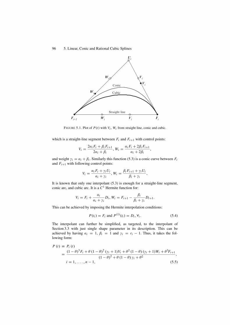
96 5. Linear, Conic and Rational Cubic Splines
Vi
Vi Fi
Vi
Ui
Wi
Wi
Wi
Fi+1
Cubic
Conic
Straight line
FIGURE 5.1. Plot of P(t) with Vi , Wi from straight line, conic and cubic.
which is a straight-line segment between Fi and Fi+1 with control points:
Vi = 2αi Fi + βi Fi+1
2αi + βi, Wi = αi Fi + 2βi Fi+1
αi + 2βi,
and weight γi = αi + βi . Similarly this function (5.3) is a conic curve between Fiand Fi+1 with following control points:
Vi = αi Fi + γiUi
αi + γi, Wi = βi Fi+1 + γiUi
βi + γi,
It is known that only one interpolant (5.3) is enough for a straight-line segment,conic arc, and cubic arc. It is a C1 Hermite function for:
Vi = Fi + αi
αi + γiDi , Wi = Fi+1 − βi
βi + γiDi+1.
This can be achieved by imposing the Hermite interpolation conditions:
P(ti ) = Fi and P(1)(ti ) = Di ,∀i . (5.4)
The interpolant can further be simplified, as targeted, to the interpolant ofSection 3.3 with just single shape parameter in its description. This can beachieved by having αi = 1, βi = 1 and γi = ri − 1. Thus, it takes the fol-lowing form:
P (t) ≡ Pi (t)
= (1 − θ)3 Fi + θ (1 − θ)2 (γi + 1)Vi + θ2 (1 − θ) (γi + 1)Wi + θ3Fi+1
(1 − θ)2 + θ (1 − θ) γi + θ2,
i = 1, . . . . , n − 1, (5.5)
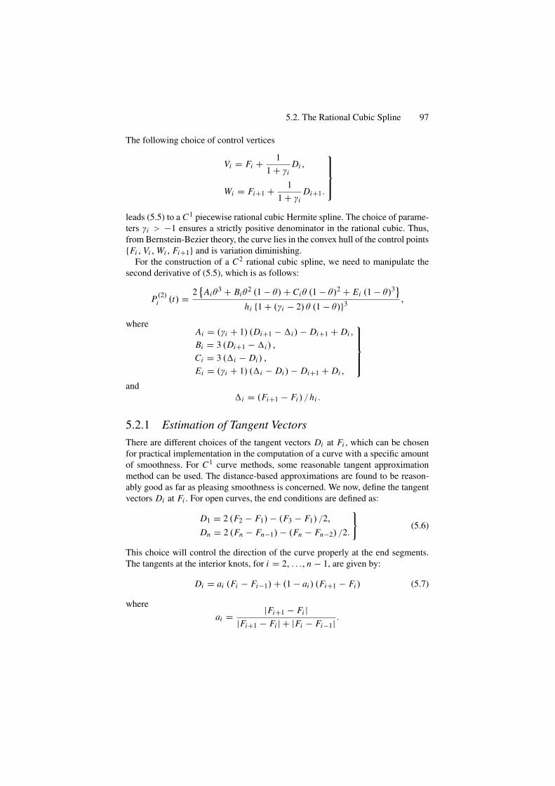
5.2. The Rational Cubic Spline 97
The following choice of control vertices
Vi = Fi + 11 + γi
Di ,
Wi = Fi+1 + 11 + γi
Di+1.
⎫⎪⎪⎬
⎪⎪⎭
leads (5.5) to a C1 piecewise rational cubic Hermite spline. The choice of parame-ters γi > −1 ensures a strictly positive denominator in the rational cubic. Thus,from Bernstein-Bezier theory, the curve lies in the convex hull of the control points{Fi , Vi , Wi , Fi+1} and is variation diminishing.
For the construction of a C2 rational cubic spline, we need to manipulate thesecond derivative of (5.5), which is as follows:
P(2)i (t) = 2
{Aiθ
3 + Biθ2 (1 − θ) + Ciθ (1 − θ)2 + Ei (1 − θ)3}
hi {1 + (γi − 2) θ (1 − θ)}3 ,
whereAi = (γi + 1) (Di+1 − �i ) − Di+1 + Di ,
Bi = 3 (Di+1 − �i ) ,
Ci = 3 (�i − Di ) ,
Ei = (γi + 1) (�i − Di ) − Di+1 + Di ,
⎫⎪⎪⎪⎬
⎪⎪⎪⎭
and�i = (Fi+1 − Fi ) /hi .
5.2.1 Estimation of Tangent VectorsThere are different choices of the tangent vectors Di at Fi , which can be chosenfor practical implementation in the computation of a curve with a specific amountof smoothness. For C1 curve methods, some reasonable tangent approximationmethod can be used. The distance-based approximations are found to be reason-ably good as far as pleasing smoothness is concerned. We now, define the tangentvectors Di at Fi . For open curves, the end conditions are defined as:
D1 = 2 (F2 − F1) − (F3 − F1) /2,
Dn = 2 (Fn − Fn−1) − (Fn − Fn−2) /2.
}
(5.6)
This choice will control the direction of the curve properly at the end segments.The tangents at the interior knots, for i = 2, . . ., n − 1, are given by:
Di = ai (Fi − Fi−1) + (1 − ai ) (Fi+1 − Fi ) (5.7)
whereai = |Fi+1 − Fi |
|Fi+1 − Fi | + |Fi − Fi−1| .
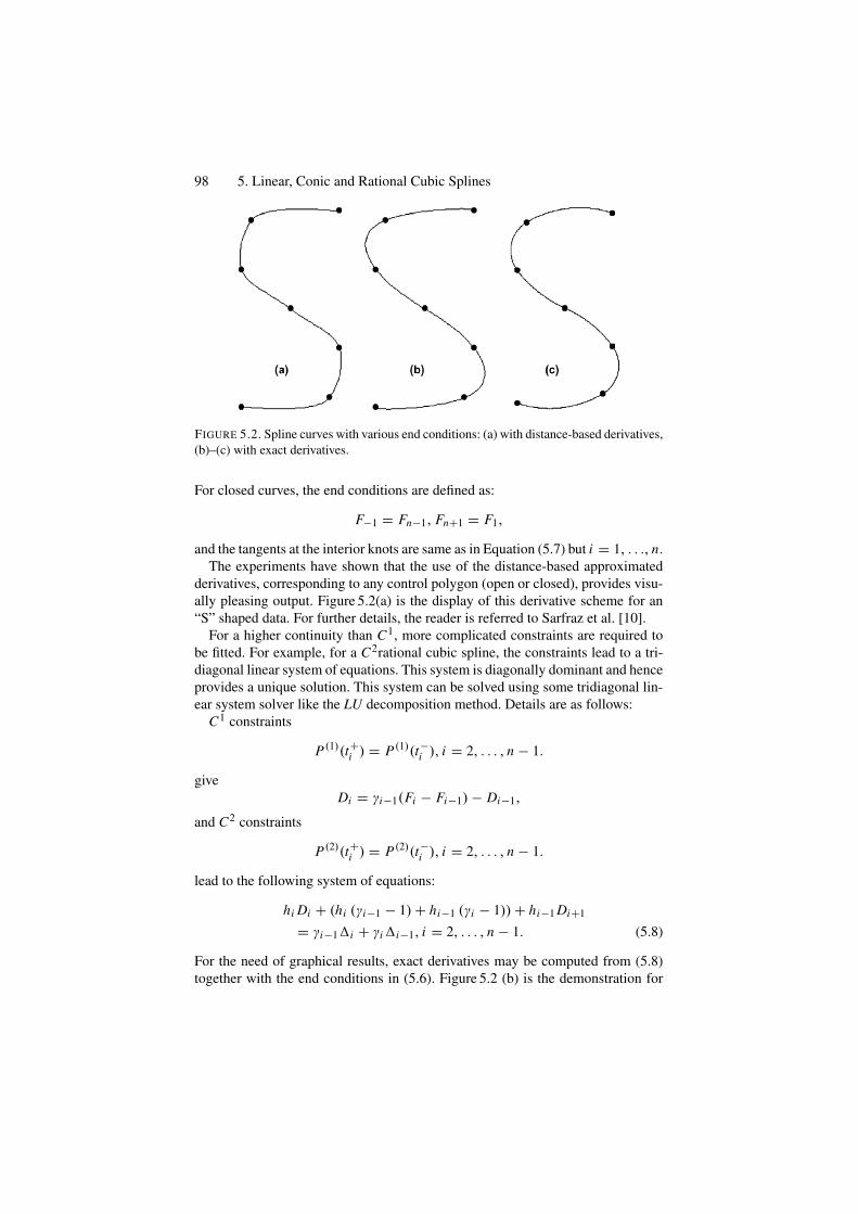
98 5. Linear, Conic and Rational Cubic Splines
FIGURE 5.2. Spline curves with various end conditions: (a) with distance-based derivatives,(b)–(c) with exact derivatives.
For closed curves, the end conditions are defined as:
F−1 = Fn−1, Fn+1 = F1,
and the tangents at the interior knots are same as in Equation (5.7) but i = 1, . . ., n.The experiments have shown that the use of the distance-based approximated
derivatives, corresponding to any control polygon (open or closed), provides visu-ally pleasing output. Figure 5.2(a) is the display of this derivative scheme for an“S” shaped data. For further details, the reader is referred to Sarfraz et al. [10].
For a higher continuity than C1, more complicated constraints are required tobe fitted. For example, for a C2rational cubic spline, the constraints lead to a tri-diagonal linear system of equations. This system is diagonally dominant and henceprovides a unique solution. This system can be solved using some tridiagonal lin-ear system solver like the LU decomposition method. Details are as follows:
C1 constraints
P(1)(t+i ) = P(1)(t−i ), i = 2, . . . , n − 1.
giveDi = γi−1(Fi − Fi−1) − Di−1,
and C2 constraints
P(2)(t+i ) = P(2)(t−i ), i = 2, . . . , n − 1.
lead to the following system of equations:
hi Di + (hi (γi−1 − 1) + hi−1 (γi − 1)) + hi−1 Di+1
= γi−1�i + γi�i−1, i = 2, . . . , n − 1. (5.8)
For the need of graphical results, exact derivatives may be computed from (5.8)together with the end conditions in (5.6). Figure 5.2 (b) is the demonstration for
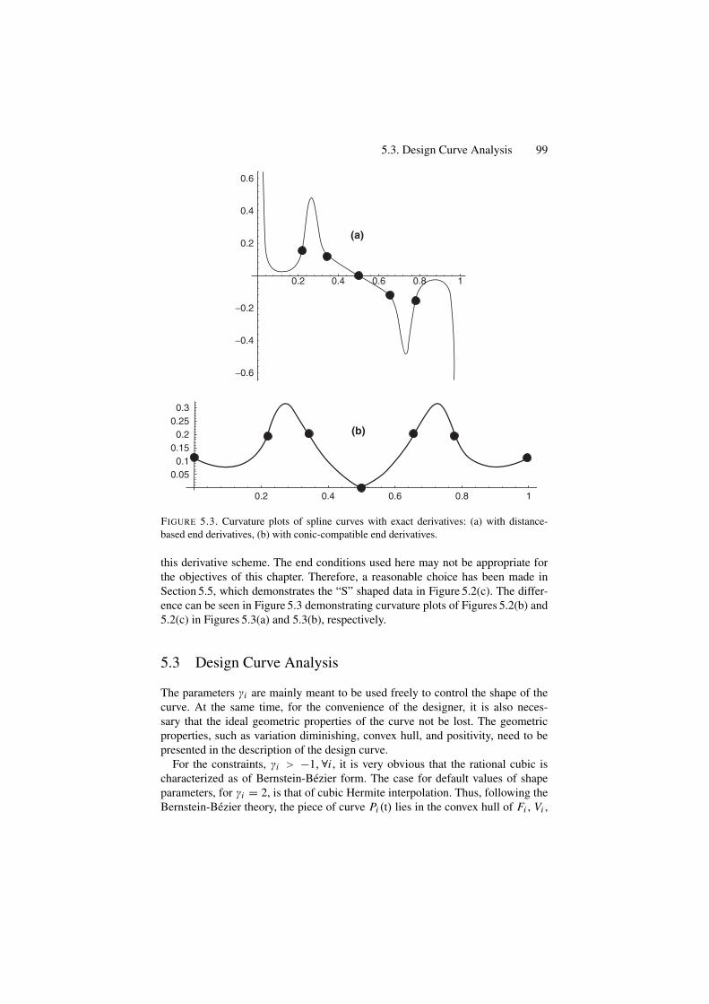
5.3. Design Curve Analysis 99
0.2
0.2
0.05
0.15
0.25
0.1
0.2
0.3
0.4 0.6 0.8 1
0.6
0.4
(a)
(b)
0.2
−0.2
−0.4
−0.6
0.4 0.6 0.8 1
FIGURE 5.3. Curvature plots of spline curves with exact derivatives: (a) with distance-based end derivatives, (b) with conic-compatible end derivatives.
this derivative scheme. The end conditions used here may not be appropriate forthe objectives of this chapter. Therefore, a reasonable choice has been made inSection 5.5, which demonstrates the “S” shaped data in Figure 5.2(c). The differ-ence can be seen in Figure 5.3 demonstrating curvature plots of Figures 5.2(b) and5.2(c) in Figures 5.3(a) and 5.3(b), respectively.
5.3 Design Curve Analysis
The parameters γi are mainly meant to be used freely to control the shape of thecurve. At the same time, for the convenience of the designer, it is also neces-sary that the ideal geometric properties of the curve not be lost. The geometricproperties, such as variation diminishing, convex hull, and positivity, need to bepresented in the description of the design curve.
For the constraints, γi > −1,∀i , it is very obvious that the rational cubic ischaracterized as of Bernstein-Bezier form. The case for default values of shapeparameters, for γi = 2, is that of cubic Hermite interpolation. Thus, following theBernstein-Bezier theory, the piece of curve Pi (t) lies in the convex hull of Fi , Vi ,
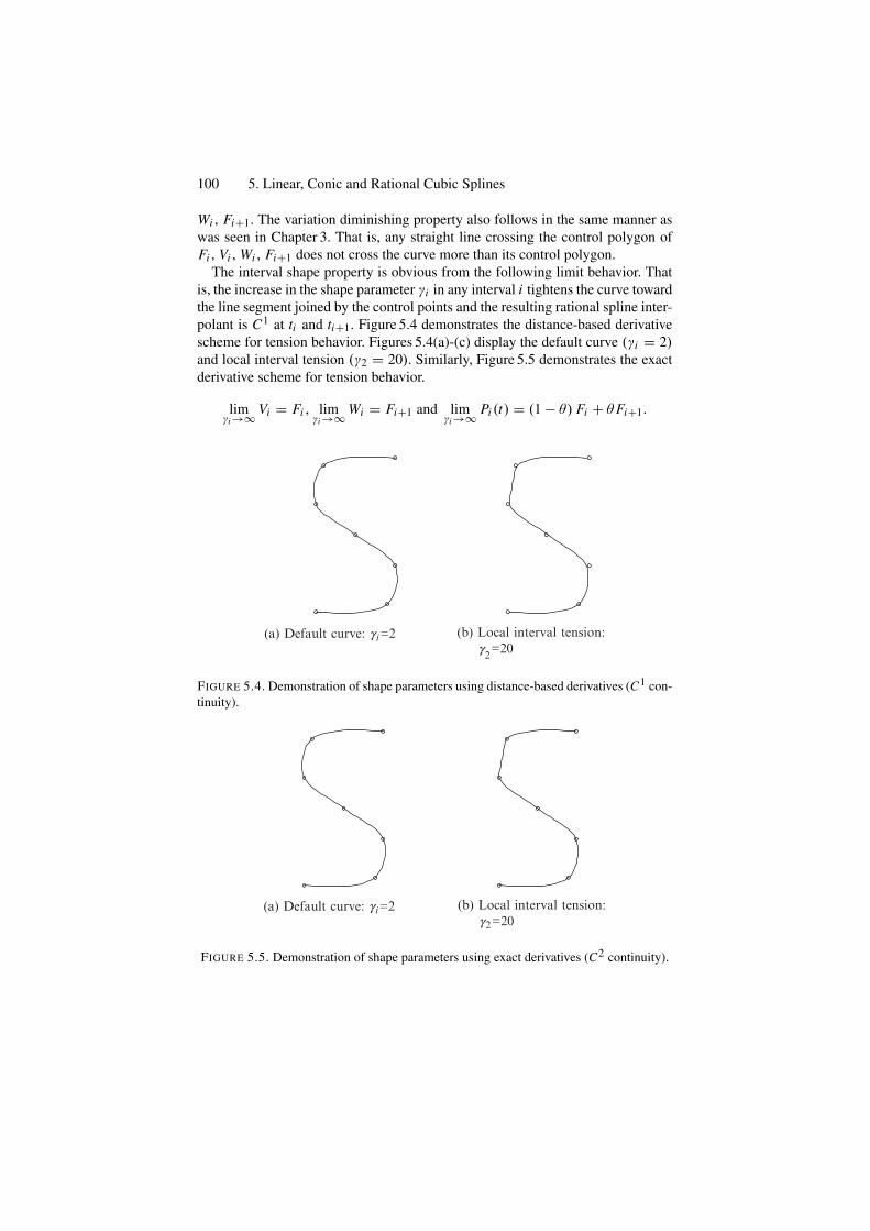
100 5. Linear, Conic and Rational Cubic Splines
Wi , Fi+1. The variation diminishing property also follows in the same manner aswas seen in Chapter 3. That is, any straight line crossing the control polygon ofFi , Vi , Wi , Fi+1 does not cross the curve more than its control polygon.
The interval shape property is obvious from the following limit behavior. Thatis, the increase in the shape parameter γi in any interval i tightens the curve towardthe line segment joined by the control points and the resulting rational spline inter-polant is C1 at ti and ti+1. Figure 5.4 demonstrates the distance-based derivativescheme for tension behavior. Figures 5.4(a)-(c) display the default curve (γi = 2)and local interval tension (γ2 = 20). Similarly, Figure 5.5 demonstrates the exactderivative scheme for tension behavior.
limγi →∞ Vi = Fi , lim
γi →∞ Wi = Fi+1 and limγi →∞ Pi (t) = (1 − θ) Fi + θ Fi+1.
(a) Default curve: g i=2 (b) Local interval tension: g2=20
FIGURE 5.4. Demonstration of shape parameters using distance-based derivatives (C1 con-tinuity).
(a) Default curve: g i=2 (b) Local interval tension: g2=20
FIGURE 5.5. Demonstration of shape parameters using exact derivatives (C2 continuity).
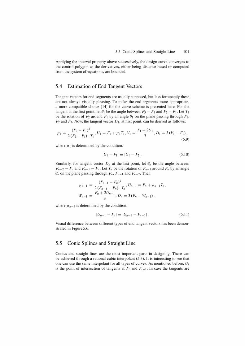
5.5. Conic Splines and Straight Line 101
Applying the interval property above successively, the design curve converges tothe control polygon as the derivatives, either being distance-based or computedfrom the system of equations, are bounded.
5.4 Estimation of End Tangent Vectors
Tangent vectors for end segments are usually supposed, but less fortunately theseare not always visually pleasing. To make the end segments more appropriate,a more compatible choice [14] for the curve scheme is presented here. For thetangent at the first point, let θ1 be the angle between F3 − F1 and F2 − F1. Let T1be the rotation of F2 around F1 by an angle θ1 on the plane passing through F1,F2 and F3. Now, the tangent vector D1, at first point, can be derived as follows:
µ1 = (F2 − F1)2
2 (F2 − F1) · T1, U1 = F1 + µ1T1, V1 = F1 + 2U1
3, D1 = 3 (V1 − F1) ,
(5.9)where µ1 is determined by the condition:
|U1 − F1| = |U1 − F2| . (5.10)
Similarly, for tangent vector Dn at the last point, let θn be the angle betweenFn−2 − Fn and Fn−1 − Fn . Let Tn be the rotation of Fn−1 around Fn by an angleθn on the plane passing through Fn , Fn−1 and Fn−2. Then
µn−1 = (Fn−1 − Fn)2
2 (Fn−1 − Fn) · Tn, Un−1 = Fn + µn−1Tn,
Wn−1 = Fn + 2Un−1
3, Dn = 3 (Fn − Wn−1) ,
where µn−1 is determined by the condition:
|Un−1 − Fn| = |Un−1 − Fn−1| . (5.11)
Visual difference between different types of end tangent vectors has been demon-strated in Figure 5.6.
5.5 Conic Splines and Straight Line
Conics and straight-lines are the most important parts in designing. These canbe achieved through a rational cubic interpolant (5.3). It is interesting to see thatone can use the same interpolant for all types of curves. As mentioned before, Uiis the point of intersection of tangents at Fi and Fi+1. In case the tangents are
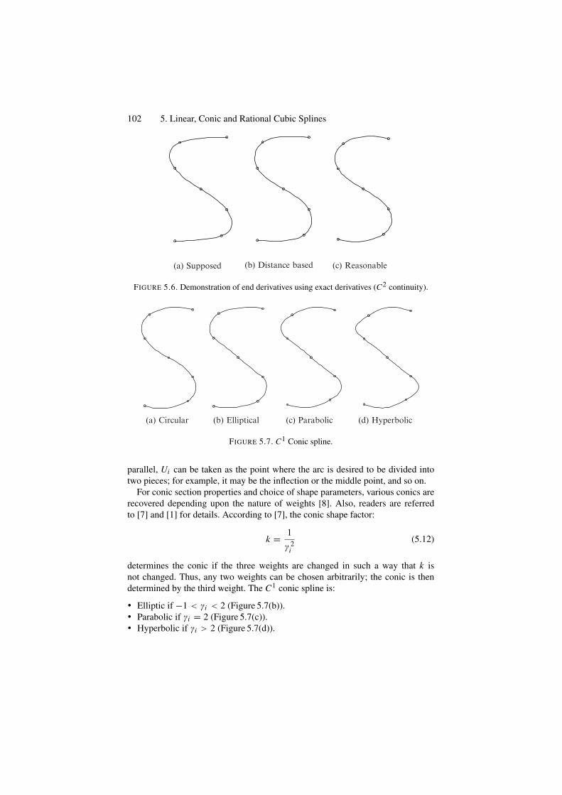
102 5. Linear, Conic and Rational Cubic Splines
(a) Supposed (b) Distance based (c) Reasonable
FIGURE 5.6. Demonstration of end derivatives using exact derivatives (C2 continuity).
(a) Circular (b) Elliptical (c) Parabolic (d) Hyperbolic
FIGURE 5.7. C1 Conic spline.
parallel, Ui can be taken as the point where the arc is desired to be divided intotwo pieces; for example, it may be the inflection or the middle point, and so on.
For conic section properties and choice of shape parameters, various conics arerecovered depending upon the nature of weights [8]. Also, readers are referredto [7] and [1] for details. According to [7], the conic shape factor:
k = 1γ 2
i(5.12)
determines the conic if the three weights are changed in such a way that k isnot changed. Thus, any two weights can be chosen arbitrarily; the conic is thendetermined by the third weight. The C1 conic spline is:
• Elliptic if −1 < γi < 2 (Figure 5.7(b)).• Parabolic if γi = 2 (Figure 5.7(c)).• Hyperbolic if γi > 2 (Figure 5.7(d)).
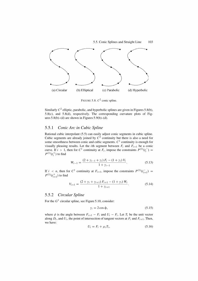
5.5. Conic Splines and Straight Line 103
FIGURE 5.8. C2 conic spline.
Similarly C2 elliptic, parabolic, and hyperbolic splines are given in Figures 5.8(b),5.8(c), and 5.8(d), respectively. The corresponding curvature plots of Fig-ures 5.8(b)–(d) are shown in Figures 5.9(b)–(d).
5.5.1 Conic Arc in Cubic SplineRational cubic interpolant (5.5) can easily adjust conic segments in cubic spline.Cubic segments are already joined by C2 continuity but there is also a need forsome smoothness between conic and cubic segments. C1 continuity is enough forvisually pleasing results. Let the i th segment between Fi and Fi+1 be a coniccurve. If i > 1, then for C1 continuity at Fi , impose the constraints P(1)(t−i ) =P(1)(t+i ) to find
Wi−1 = (2 + γi−1 + γi ) Fi − (1 + γi ) Vi
1 + γi−1. (5.13)
If i < n, then for C1 continuity at Fi+1, impose the constraints P(1)(t−i+1) =P(1)(t+i+1) to find
Vi+1 = (2 + γi + γi+1) Fi+1 − (1 + γi ) Wi
1 + γi+1. (5.14)
5.5.2 Circular SplineFor the G1 circular spline, see Figure 5.10, consider:
γi = 2 cos φ, (5.15)
where φ is the angle between Fi+1 − Fi and Ui − Fi . Let Ti be the unit vectoralong Di , and Ui , the point of intersection of tangent vectors at Fi and Fi+1. Then,we have:
Ui = Fi + µi Ti , (5.16)
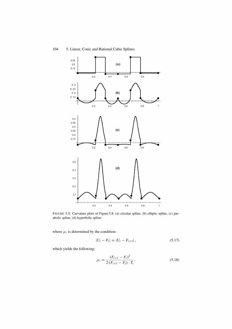
104 5. Linear, Conic and Rational Cubic Splines
0.25
0.2
0.15
0.2 0.4 0.6 0.8
(a)
0.25
0.3
0.2
0.15
0.2 0.4 0.6 0.8 1
(b)
(c)
0.4
0.35
0.3
0.25
0.2
0.15
0.2 0.4 0.6 0.8
0.5
0.1
0.2
0.3
0.4
0.2 0.4 0.6 0.8 1
(d)
FIGURE 5.9. Curvature plots of Figure 5.8: (a) circular spline, (b) elliptic spline, (c) par-abolic spline, (d) hyperbolic spline.
where µi is determined by the condition:
|Ui − Fi | = |Ui − Fi+1| , (5.17)
which yields the following:
µi = (Fi+1 − Fi )2
2 (Fi+1 − Fi ) · Ti. (5.18)
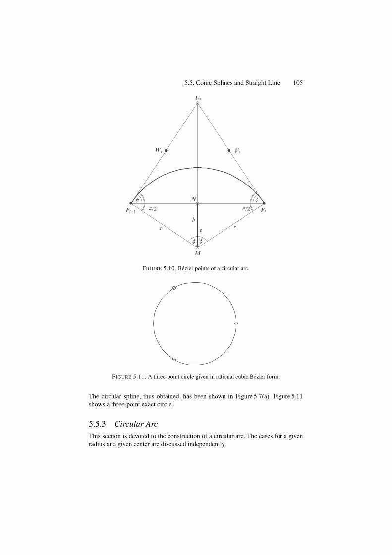
5.5. Conic Splines and Straight Line 105
FiFi+1
ViWi
Ui
N
M
er rb
f f
f f
p/2 p/2
FIGURE 5.10. Bezier points of a circular arc.
FIGURE 5.11. A three-point circle given in rational cubic Bezier form.
The circular spline, thus obtained, has been shown in Figure 5.7(a). Figure 5.11shows a three-point exact circle.
5.5.3 Circular ArcThis section is devoted to the construction of a circular arc. The cases for a givenradius and given center are discussed independently.
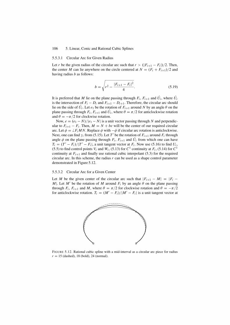
106 5. Linear, Conic and Rational Cubic Splines
5.5.3.1 Circular Arc for Given Radius
Let r be the given radius of the circular arc such that r > (|Fi+1 − Fi |)/2. Then,the center M can lie anywhere on the circle centered at N = (Fi + Fi+1)/2 andhaving radius b as follows:
b =√
r2 − |Fi+1 − Fi |24
. (5.19)
It is preferred that M lie on the plane passing through Fi , Fi+1 and Ui , where Uiis the intersection of Fi − Di and Fi+1 − Di+1. Therefore, the circular arc shouldlie on the side of Ui . Let e1 be the rotation of Fi+1 around N by an angle θ on theplane passing through Fi , Fi+1 and Ui , where θ = π/2 for anticlockwise rotationand θ = −π/2 for clockwise rotation.
Now, e = (e1 − N )/|e1 − N | is a unit vector passing through N and perpendic-ular to Fi+1 − Fi . Then, M = N + be will be the center of our required circulararc. Let φ = Fi M N . Replace φ with −φ if circular arc rotation is anticlockwise.Next, one can find γi from (5.15). Let T ′ be the rotation of Fi+1 around Fi throughangle φ on the plane passing through Fi , Fi+1 and Ui from which one can haveTi = (T ′ − Fi )/|T ′ − Fi |, a unit tangent vector at Fi . Now use (5.16) to find Ui ,(5.5) to find control points Vi and Wi , (5.13) for C1 continuity at Fi , (5.14) for C1
continuity at Fi+1 and finally use rational cubic interpolant (5.3) for the requiredcircular arc. In this scheme, the radius r can be used as a shape control parameterdemonstrated in Figure 5.12.
5.5.3.2 Circular Arc for a Given Center
Let M be the given center of the circular arc such that |Fi+1 − M | = |Fi −M |. Let M ′ be the rotation of M around Fi by an angle θ on the plane passingthrough Fi , Fi+1 and M , where θ = π/2 for clockwise rotation and θ = −π/2for anticlockwise rotation. Ti = (M ′ − Fi )/|M ′ − Fi | is a unit tangent vector at
FIGURE 5.12. Rational cubic spline with a mid-interval as a circular arc piece for radiusr = 15 (dashed), 18 (bold), 24 (normal).
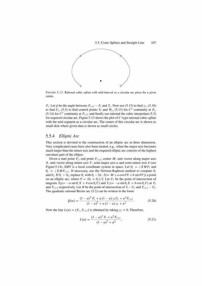
5.5. Conic Splines and Straight Line 107
FIGURE 5.13. Rational cubic spline with mid-interval as a circular arc piece for a givencenter.
Fi . Let φ be the angle between Fi+1 − Fi and Ti . Now use (5.15) to find γi , (5.16)to find Ui , (5.5) to find control points Vi and Wi , (5.13) for C1 continuity at Fi ,(5.14) for C1 continuity at Fi+1 and finally use rational the cubic interpolant (5.3)for required circular arc. Figure 5.13 shows the plot of C-type rational cubic splinewith the mid-segment as a circular arc. The center of this circular arc is shown assmall disk where given data is shown as small circles.
5.5.4 Elliptic ArcThis section is devoted to the construction of an elliptic arc in three dimension.Very complicated cases have also been treated, e.g., when the major axis becomesmuch larger than the minor axis and the required elliptic arc consists of the highestcurvature part of the ellipse.
Given a start point Fi , end point Fi+1, center M , unit vector along major axisX , unit vector along minor axis Y , semi-major axis a and semi-minor axis b (seeFigure 5.14), XMY is a local coordinate system in space. Let θs = X M Fi andθe = X M Fi+1. If necessary, use the Newton-Raphson method to compute θsand θe. If θs > θe, replace θs with θs −2π . S(= M +a cos θ X +b sin θY }) a pointon an elliptic arc, where θ = (θs + θe)/2. Let Ui be the point of intersection oftangents T0(= −a sin θs X + b cos θsY ) and T1(= −a sin θe X + b cos θeY ) at Fiand Fi+1 respectively. Let R be the point of intersection of S − Ui and Fi+1 − Fi .The quadratic rational Bezier arc (5.2) can be written in the form:
Q(u) = (1 − u)2 Fi + u (1 − u) γiUi + u2 Fi+1
(1 − u)2 + u (1 − u) γi + u2. (5.20)
Now the line L(u) = [Fi , Fi+1] is obtained by taking γi = 0. Therefore,
L(u) = (1 − u)2 Fi + u2 Fi+1
(1 − u)2 + u2, (5.21)
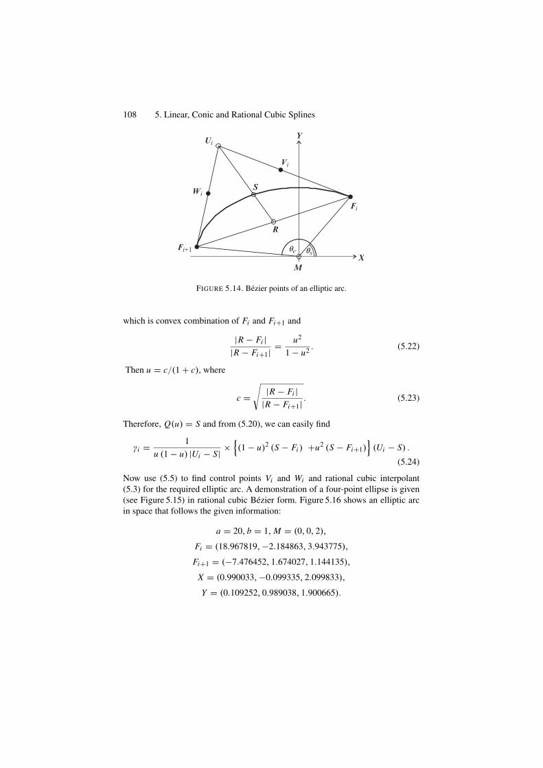
108 5. Linear, Conic and Rational Cubic Splines
Fi
Fi+1
Vi
Wi
MX
YUi
R
S
qe qs
FIGURE 5.14. Bezier points of an elliptic arc.
which is convex combination of Fi and Fi+1 and
|R − Fi ||R − Fi+1| = u2
1 − u2 . (5.22)
Then u = c/(1 + c), where
c =√
|R − Fi ||R − Fi+1| . (5.23)
Therefore, Q(u) = S and from (5.20), we can easily find
γi = 1u (1 − u) |Ui − S| ×
{(1 − u)2 (S − Fi ) +u2 (S − Fi+1)
}(Ui − S) .
(5.24)
Now use (5.5) to find control points Vi and Wi and rational cubic interpolant(5.3) for the required elliptic arc. A demonstration of a four-point ellipse is given(see Figure 5.15) in rational cubic Bezier form. Figure 5.16 shows an elliptic arcin space that follows the given information:
a = 20, b = 1, M = (0, 0, 2),
Fi = (18.967819,−2.184863, 3.943775),
Fi+1 = (−7.476452, 1.674027, 1.144135),
X = (0.990033,−0.099335, 2.099833),
Y = (0.109252, 0.989038, 1.900665).
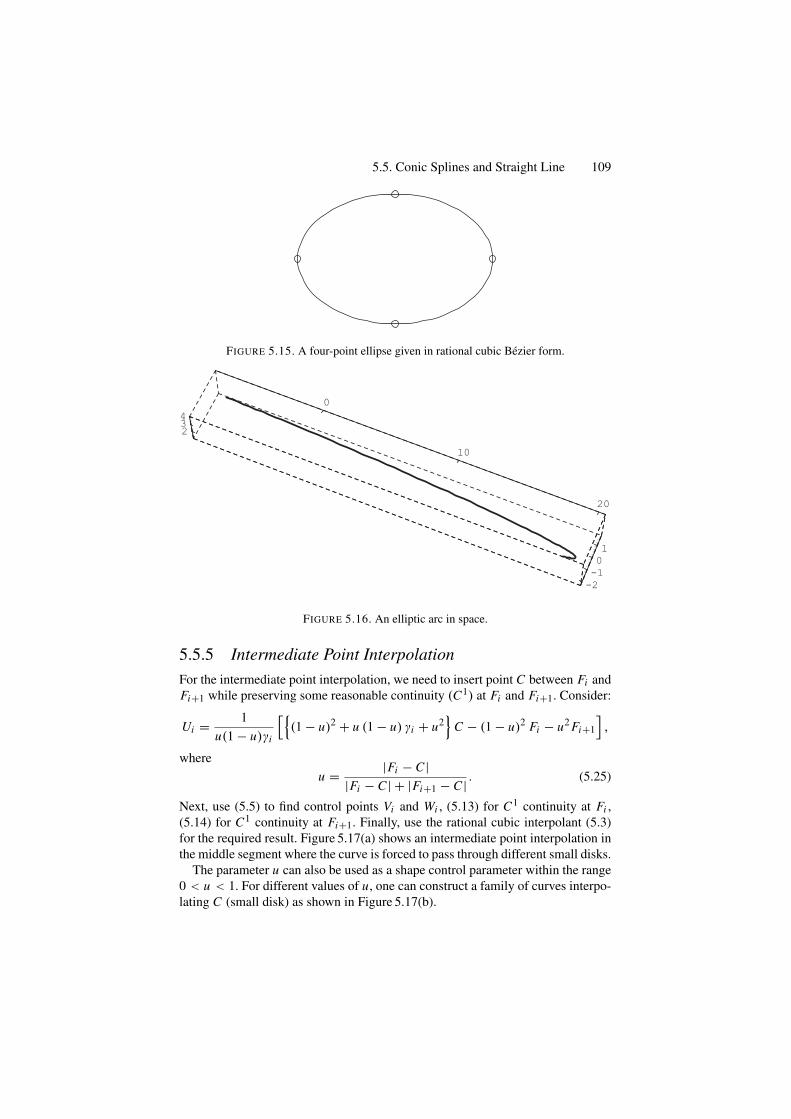
5.5. Conic Splines and Straight Line 109
FIGURE 5.15. A four-point ellipse given in rational cubic Bezier form.
0
10
20
-2-101
234
FIGURE 5.16. An elliptic arc in space.
5.5.5 Intermediate Point InterpolationFor the intermediate point interpolation, we need to insert point C between Fi andFi+1 while preserving some reasonable continuity (C1) at Fi and Fi+1. Consider:
Ui = 1u(1 − u)γi
[{(1 − u)2 + u (1 − u) γi + u2
}C − (1 − u)2 Fi − u2 Fi+1
],
whereu = |Fi − C |
|Fi − C | + |Fi+1 − C | . (5.25)
Next, use (5.5) to find control points Vi and Wi , (5.13) for C1 continuity at Fi ,(5.14) for C1 continuity at Fi+1. Finally, use the rational cubic interpolant (5.3)for the required result. Figure 5.17(a) shows an intermediate point interpolation inthe middle segment where the curve is forced to pass through different small disks.
The parameter u can also be used as a shape control parameter within the range0 < u < 1. For different values of u, one can construct a family of curves interpo-lating C (small disk) as shown in Figure 5.17(b).
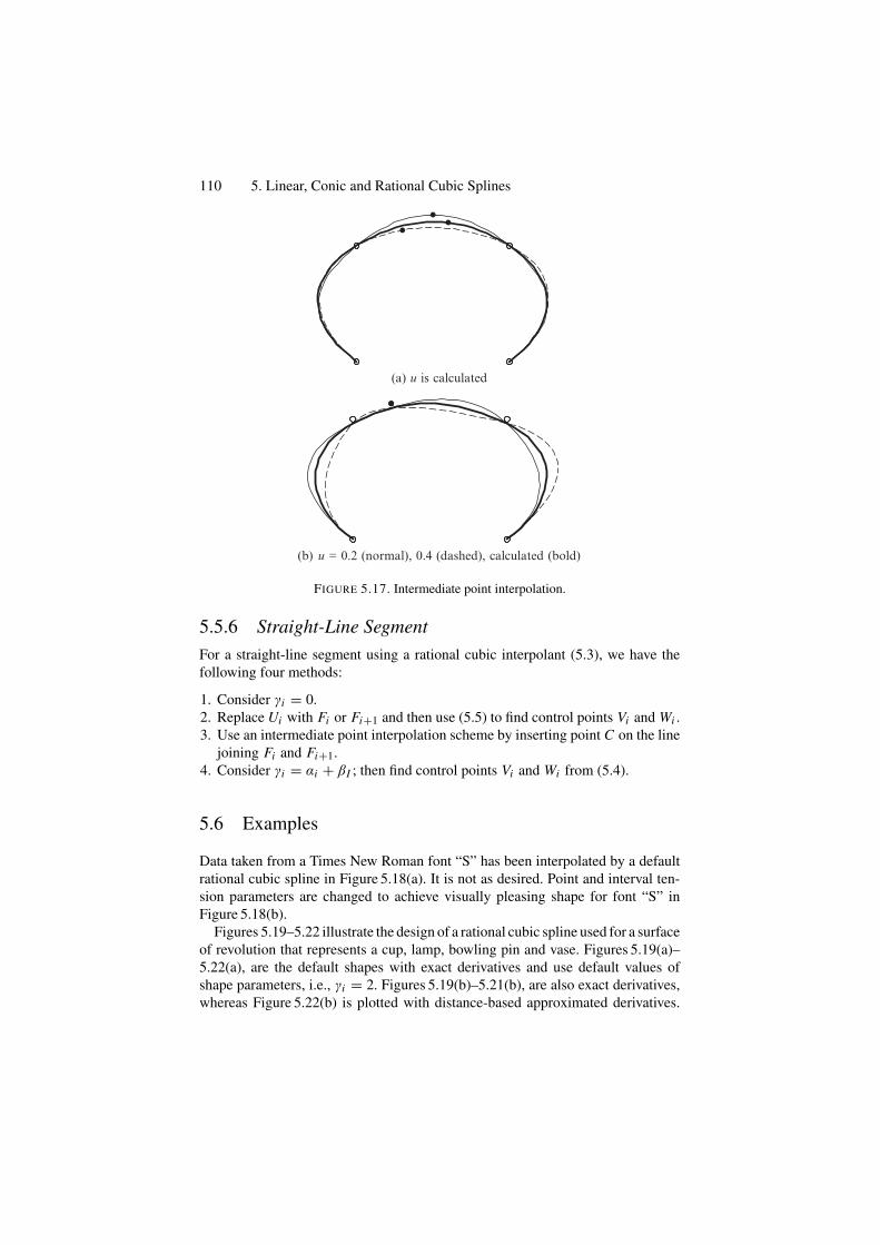
110 5. Linear, Conic and Rational Cubic Splines
(a) u is calculated
(b) u = 0.2 (normal), 0.4 (dashed), calculated (bold)
FIGURE 5.17. Intermediate point interpolation.
5.5.6 Straight-Line SegmentFor a straight-line segment using a rational cubic interpolant (5.3), we have thefollowing four methods:
1. Consider γi = 0.2. Replace Ui with Fi or Fi+1 and then use (5.5) to find control points Vi and Wi .3. Use an intermediate point interpolation scheme by inserting point C on the line
joining Fi and Fi+1.4. Consider γi = αi + βI ; then find control points Vi and Wi from (5.4).
5.6 Examples
Data taken from a Times New Roman font “S” has been interpolated by a defaultrational cubic spline in Figure 5.18(a). It is not as desired. Point and interval ten-sion parameters are changed to achieve visually pleasing shape for font “S” inFigure 5.18(b).
Figures 5.19–5.22 illustrate the design of a rational cubic spline used for a surfaceof revolution that represents a cup, lamp, bowling pin and vase. Figures 5.19(a)–5.22(a), are the default shapes with exact derivatives and use default values ofshape parameters, i.e., γi = 2. Figures 5.19(b)–5.21(b), are also exact derivatives,whereas Figure 5.22(b) is plotted with distance-based approximated derivatives.
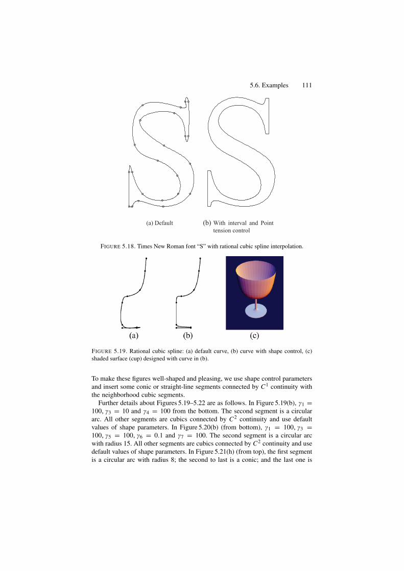
5.6. Examples 111
(a) Default (b) With interval and Point
tension control
FIGURE 5.18. Times New Roman font “S” with rational cubic spline interpolation.
FIGURE 5.19. Rational cubic spline: (a) default curve, (b) curve with shape control, (c)shaded surface (cup) designed with curve in (b).
To make these figures well-shaped and pleasing, we use shape control parametersand insert some conic or straight-line segments connected by C1 continuity withthe neighborhood cubic segments.
Further details about Figures 5.19–5.22 are as follows. In Figure 5.19(b), γ1 =100, γ3 = 10 and γ4 = 100 from the bottom. The second segment is a circulararc. All other segments are cubics connected by C2 continuity and use defaultvalues of shape parameters. In Figure 5.20(b) (from bottom), γ1 = 100, γ3 =100, γ5 = 100, γ6 = 0.1 and γ7 = 100. The second segment is a circular arcwith radius 15. All other segments are cubics connected by C2 continuity and usedefault values of shape parameters. In Figure 5.21(h) (from top), the first segmentis a circular arc with radius 8; the second to last is a conic; and the last one is
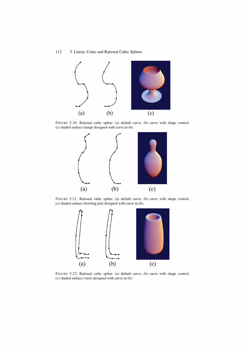
112 5. Linear, Conic and Rational Cubic Splines
FIGURE 5.20. Rational cubic spline: (a) default curve, (b) curve with shape control,(c) shaded surface (lamp) designed with curve in (b).
FIGURE 5.21. Rational cubic spline: (a) default curve, (b) curve with shape control,(c) shaded surface (bowling pin) designed with curve in (b).
FIGURE 5.22. Rational cubic spline: (a) default curve, (b) curve with shape control,(c) shaded surface (vase) designed with curve in (b).
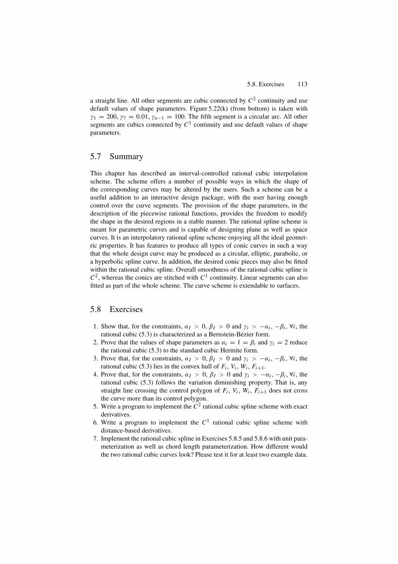
5.8. Exercises 113
a straight line. All other segments are cubic connected by C2 continuity and usedefault values of shape parameters. Figure 5.22(k) (from bottom) is taken withγ1 = 200, γ7 = 0.01, γn−1 = 100. The fifth segment is a circular arc. All othersegments are cubics connected by C1 continuity and use default values of shapeparameters.
5.7 Summary
This chapter has described an interval-controlled rational cubic interpolationscheme. The scheme offers a number of possible ways in which the shape ofthe corresponding curves may be altered by the users. Such a scheme can be auseful addition to an interactive design package, with the user having enoughcontrol over the curve segments. The provision of the shape parameters, in thedescription of the piecewise rational functions, provides the freedom to modifythe shape in the desired regions in a stable manner. The rational spline scheme ismeant for parametric curves and is capable of designing plane as well as spacecurves. It is an interpolatory rational spline scheme enjoying all the ideal geomet-ric properties. It has features to produce all types of conic curves in such a waythat the whole design curve may be produced as a circular, elliptic, parabolic, ora hyperbolic spline curve. In addition, the desired conic pieces may also be fittedwithin the rational cubic spline. Overall smoothness of the rational cubic spline isC2, whereas the conics are stitched with C1 continuity. Linear segments can alsofitted as part of the whole scheme. The curve scheme is extendable to surfaces.
5.8 Exercises
1. Show that, for the constraints, αI > 0, βI > 0 and γi > −αi , −βi , ∀i , therational cubic (5.3) is characterized as a Bernstein-Bezier form.
2. Prove that the values of shape parameters as αi = 1 = βi and γi = 2 reducethe rational cubic (5.3) to the standard cubic Hermite form.
3. Prove that, for the constraints, αI > 0, βI > 0 and γi > −αi , −βi , ∀i , therational cubic (5.3) lies in the convex hull of Fi , Vi , Wi , Fi+1.
4. Prove that, for the constraints, αI > 0, βI > 0 and γi > −αi ,−βi ,∀i , therational cubic (5.3) follows the variation diminishing property. That is, anystraight line crossing the control polygon of Fi , Vi , Wi , Fi+1 does not crossthe curve more than its control polygon.
5. Write a program to implement the C2 rational cubic spline scheme with exactderivatives.
6. Write a program to implement the C1 rational cubic spline scheme withdistance-based derivatives.
7. Implement the rational cubic spline in Exercises 5.8.5 and 5.8.6 with unit para-meterization as well as chord length parameterization. How different wouldthe two rational cubic curves look? Please test it for at least two example data.
114 5. Linear, Conic and Rational Cubic Splines
8. Write a program to implement the rational cubic spline scheme withdistance-based derivatives but resulting in an elliptic curve.
9. Write a program to implement the rational cubic spline scheme withdistance-based derivatives but resulting in a hyperbolic curve.
10. Write a program to implement the rational cubic spline scheme with distance-based derivatives but resulting in a parabolic curve.
11. Write a program to implement the rational cubic spline scheme with distance-based derivatives but resulting in a curve with circular pieces.
12. Write a program for the C2 rational cubic spline which, in addition to passingthrough the regular data points, can also pass through another desired datapoint(s) in some desired piece(s).
13. Derive the tridiagonal linear system of equations by imposing the constraintsfor C2 continuity
P(2)(t−i) = P(2)
(t+i), i = 2, 3, . . . , n − 1
on rational cubic function P(t) in (5.3) with control points in (5.5).14. Write a program to solve the tridiagonal linear system of equations in Exercise
5.8.13 by LU-factorization to find the values of exact derivatives Di , i =2, . . ., n − 1 by estimation of appropriate end derivatives.
15. Write an algorithm to implement the rational cubic spline scheme for closeddata.
16. Find the equation in (5.15) for the quadratic rational function Q(t) to be acircular arc with condition in (5.17).
17. Derive the formula for intermediate point interpolation in Section 5.5 to findthe value of Ui .
18. Write a program to implement the elliptic arc in three dimensions by usinggiven data in Section 5.5.
19. Prove the fact that the presented spline scheme, in this chapter, has C2 con-tinuity between the rational cubic arcs and C1 continuity between cubic andconic arcs.
20. Show, by practical implementation of Exercise 5.8.5, that the scheme is local,i.e., shape control parameters will not significantly affect the adjacent parts ofthe design curve.
21. Implement Exercises 5.8.5–5.8.8 to show that all these methods are suitablefor space curves and hence can also be generalized to surfaces.
References1. Farin, G. (1995), NURB Curves and Surfaces, A.K. Peters.2. Gregory, J.A., and Sarfraz, M. (1990), A rational spline with tension, Comput Aided
Geom Design, 7, 1–13.3. Habib, Z., and Sarfraz, M. (2001), A rational cubic spline for the visualization
of convex data, The Proceedings of IEEE International Conference on InformationVisualization-IV’01-UK, IEEE Computer Society Press, pp. 744–748.
4. Hoschek, J. (1992), Circular splines, Comput Aided Design, 24, 611–618.

References 115
5. Jamaludin, M.A., Said, H.B., and Majid, A. (1995), Shape control of parametric cubiccurves, The Proceedings of CAD/Graphics’95, China, SPIE Proceedings Series, Vol.2644, pp. 128–133.
6. Meek, D.S., Ong, B., and Walton, D.J. (2003), A constrained guided G1 continuousspline curve, Comput Aided Design, 35, 591–599.
7. Piegl, L., and Tiller, W. (1995), The NURBS Book, Springer-Verlag, New York.8. Sarfraz, M. (1995), Curves and surfaces for CAD using C2 rational cubic splines, Eng
Comput 11 (2), 94–102.9. Sarfraz, M. (2003), Optimal curve fitting to digital data, Int J WSCG, 11 (1), 128–135.
10. Sarfraz, M., and Habib, Z. (2000), Rational cubic and conic representation: a practicalapproach, IIUM Eng J, Malaysia, 1 (2), 7–15.
11. Sarfraz, M., Habib, Z., and Hussain, M. (1998), Piecewise interpolation for designingof parametric curves, The Proceedings of IEEE International Conference on Informa-tion Visualization-IV’98-UK, IEEE Computer Society Press, pp. 307–313.
12. Sarfraz, M., Hussain, M., and Habib, Z. (1997), Local convexity preserving rationalcubic spline curves, The Proceedings of IEEE International Conference on InformationVisualization-IV’97-UK, IEEE Computer Society Press, pp. 211–218.
13. Sarfraz, M. and Khan, M. (2002), Automatic outline capture of Arabic fonts, Int JInformation Sci, Elsevier Science, 140 (3–4), 269–281.
14. Habib, Z., Sakai, M., and Sarfraz, M. (2004), Interactive shape control with rationalcubic splines, Int J Comput Aided Design Appl, 1(1–4), 709–718.
6Shape-Preserving Rational Interpolationfor Planar Curves
Abstract. Data visualization is an important issue in information visualization. In specificapplications, data may have different shapes when occurring in scientific phenomena or insome other perspective. A simple application may be when data is globally monotone orconvex. Representing data in a visually meaningful and computationally efficient way is asignificant topic to consider. This chapter deals with such situations using the piecewiserational cubic interpolant of Section 3.3. For simplicity, the shape parameters introducedin each interval have been constrained to solve the problem of shape-preserving interpo-lation for planer curves. Scalar curves are also considered as a special case, but they arediscussed in detail in Chapters 7 and 8.
6.1 Introduction
Many authors work in the area of representing shape-preserving curves for shapeddata. For brevity, the reader is referred to [1–23]. This chapter uses the piece-wise rational cubic interpolant of Section 3.3, where only one shape parameteris introduced in each interval, to solve the problem of shape-preserving interpo-lation for plane curves. The scalar curves are also considered as a special case,but their detailed versions have been discussed in details in Chapters 7 and 8. Theresults derived here are actually the extensions of the results of Delbourgo andGregory [4] who developed a C1 shape-preserving interpolation scheme for scalarcurves using the same piecewise rational function. They derived the constraints,on the shape parameters occurring in the rational function under discussion, tomake the interpolant preserve the monotonic and/or convex shape of the data.
This chapter begins with some preliminaries about the rational cubic inter-polant. The constraints with convex and/or monotonic data are derived inSections 6.3, 6.4 and 6.5. These constraints depend on the tangent vectors. Thedescription of the tangent vectors, which are consistent and dependent on thegiven data, is made in Section 6.6. The shape-preserving results are explainedwith examples in Section 6.7.
117
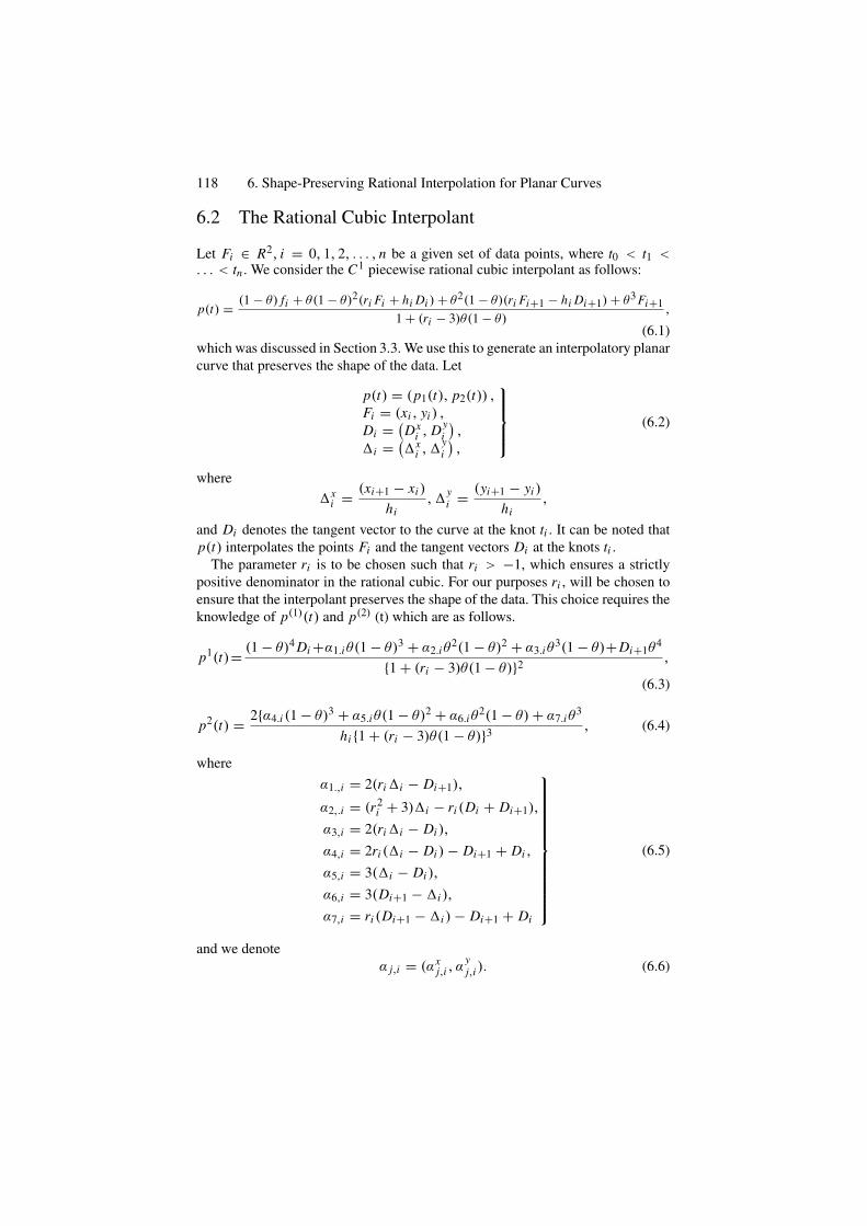
118 6. Shape-Preserving Rational Interpolation for Planar Curves
6.2 The Rational Cubic Interpolant
Let Fi ∈ R2, i = 0, 1, 2, . . . , n be a given set of data points, where t0 < t1 <. . . < tn . We consider the C1 piecewise rational cubic interpolant as follows:
p(t) = (1 − θ) fi + θ(1 − θ)2(ri Fi + hi Di ) + θ2(1 − θ)(ri Fi+1 − hi Di+1) + θ3 Fi+11 + (ri − 3)θ(1 − θ)
,
(6.1)which was discussed in Section 3.3. We use this to generate an interpolatory planarcurve that preserves the shape of the data. Let
p(t) = (p1(t), p2(t)) ,Fi = (xi , yi ) ,
Di = (Dxi , Dy
i),
�i = (�xi ,�
yi),
⎫⎪⎪⎬
⎪⎪⎭(6.2)
where�x
i = (xi+1 − xi )
hi,�
yi = (yi+1 − yi )
hi,
and Di denotes the tangent vector to the curve at the knot ti . It can be noted thatp(t) interpolates the points Fi and the tangent vectors Di at the knots ti .
The parameter ri is to be chosen such that ri > −1, which ensures a strictlypositive denominator in the rational cubic. For our purposes ri , will be chosen toensure that the interpolant preserves the shape of the data. This choice requires theknowledge of p(1)(t) and p(2) (t) which are as follows.
p1(t)= (1 − θ)4 Di +α1.iθ(1 − θ)3 + α2.iθ2(1 − θ)2 + α3.iθ
3(1 − θ)+Di+1θ4
{1 + (ri − 3)θ(1 − θ)}2 ,
(6.3)
p2(t) = 2{α4.i (1 − θ)3 + α5.iθ(1 − θ)2 + α6.iθ2(1 − θ) + α7.iθ
3
hi {1 + (ri − 3)θ(1 − θ)}3 , (6.4)
whereα1.,i = 2(ri�i − Di+1),
α2,.i = (r2i + 3)�i − ri (Di + Di+1),
α3,i = 2(ri�i − Di ),
α4,i = 2ri (�i − Di ) − Di+1 + Di ,
α5,i = 3(�i − Di ),
α6,i = 3(Di+1 − �i ),
α7,i = ri (Di+1 − �i ) − Di+1 + Di
⎫⎪⎪⎪⎪⎪⎪⎪⎪⎪⎪⎪⎬
⎪⎪⎪⎪⎪⎪⎪⎪⎪⎪⎪⎭
(6.5)
and we denoteα j,i = (αx
j,i , αyj,i ). (6.6)
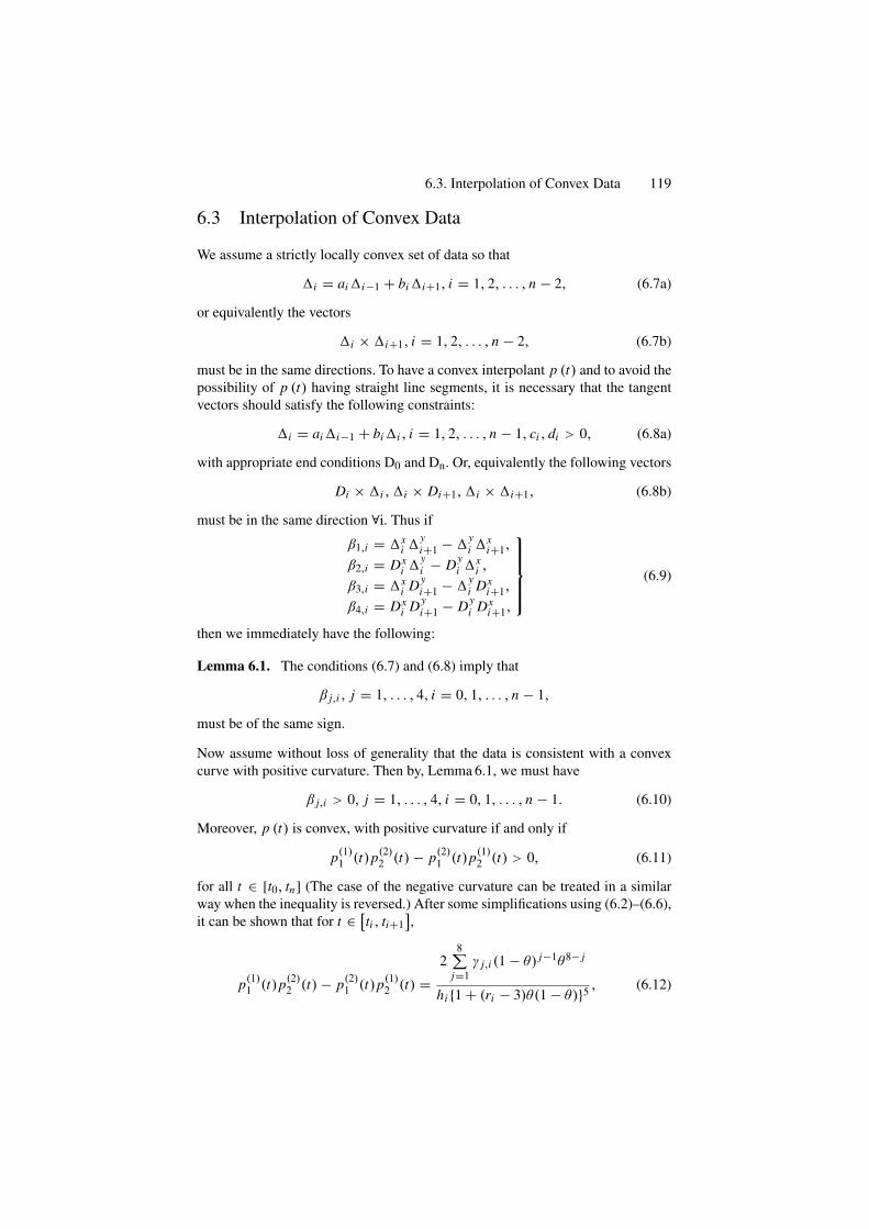
6.3. Interpolation of Convex Data 119
6.3 Interpolation of Convex Data
We assume a strictly locally convex set of data so that
�i = ai�i−1 + bi�i+1, i = 1, 2, . . . , n − 2, (6.7a)
or equivalently the vectors
�i × �i+1, i = 1, 2, . . . , n − 2, (6.7b)
must be in the same directions. To have a convex interpolant p (t) and to avoid thepossibility of p (t) having straight line segments, it is necessary that the tangentvectors should satisfy the following constraints:
�i = ai�i−1 + bi�i , i = 1, 2, . . . , n − 1, ci , di > 0, (6.8a)
with appropriate end conditions D0 and Dn. Or, equivalently the following vectors
Di × �i ,�i × Di+1,�i × �i+1, (6.8b)
must be in the same direction ∀i. Thus if
β1,i = �xi �
yi+1 − �
yi �x
i+1,
β2,i = Dxi �
yi − Dy
i �xi ,
β3,i = �xi Dy
i+1 − �yi Dx
i+1,
β4,i = Dxi Dy
i+1 − Dyi Dx
i+1,
⎫⎪⎪⎪⎬
⎪⎪⎪⎭
(6.9)
then we immediately have the following:
Lemma 6.1. The conditions (6.7) and (6.8) imply that
β j,i , j = 1, . . . , 4, i = 0, 1, . . . , n − 1,
must be of the same sign.
Now assume without loss of generality that the data is consistent with a convexcurve with positive curvature. Then by, Lemma 6.1, we must have
β j,i > 0, j = 1, . . . , 4, i = 0, 1, . . . , n − 1. (6.10)
Moreover, p (t) is convex, with positive curvature if and only if
p(1)1 (t)p(2)
2 (t) − p(2)1 (t)p(1)
2 (t) > 0, (6.11)
for all t ∈ [t0, tn] (The case of the negative curvature can be treated in a similarway when the inequality is reversed.) After some simplifications using (6.2)–(6.6),it can be shown that for t ∈ [ti , ti+1
],
p(1)1 (t)p(2)
2 (t) − p(2)1 (t)p(1)
2 (t) =2
8∑
j=1γ j,i (1 − θ) j−1θ8− j
hi {1 + (ri − 3)θ(1 − θ)}5 , (6.12)
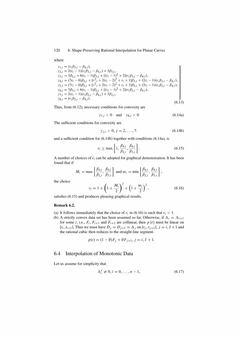
120 6. Shape-Preserving Rational Interpolation for Planar Curves
where
γ1,i = (ri β3,i − β4,i ),γ2,i = 2(ri − 1)(riβ3,i − β4,i ) + 3β3,i ,
γ3,i = 3β2,i + 6(ri − 1)β3,i + [(ri − 1)2 + 2](ri β3,i − β4,i ),
γ4,i = (7ri − 6)β2,i + [r2i + 2(ri − 2)2 + ri + 1]β3,i + (2ri − 1)(ri β3,i − β4,i ),
γ5,i = (7ri − 6)β3,i + [r2i + 2(ri − 2)2 + ri + 1]β2,i + (2ri − 1)(ri β2,i − β4,i ),
γ6,i = 3β3,i + 6(ri − 1)β2,i + [(ri − 1)2 + 2](ri β2,i − β4,i ),γ7,i = 2(ri − 1)(riβ2,i − β4,i ) + 3β2,i ,γ8,i = (ri β2,i − β4,i ).
⎫⎪⎪⎪⎪⎪⎪⎪⎪⎪⎪⎬
⎪⎪⎪⎪⎪⎪⎪⎪⎪⎪⎭
(6.13)Thus, from (6.12), necessary conditions for convexity are
γ1,i > 0 and γ8,i > 0 (6.14a)
The sufficient conditions for convexity are
γ j,i > 0, j = 2, . . . , 7. (6.14b)
and a sufficient condition for (6.14b) together with conditions (6.14a), is
ri ≥ max{
1,β4,i
β2,i,β4,i
β3,i
}. (6.15)
A number of choices of ri can be adopted for graphical demonstration. It has beenfound that if
Mi = max{
β4,i
β2,i,β4,i
β3,i
}and mi = min
{β4,i
β2,i,β4,i
β3,i
},
the choice
ri = 1 +(
1 + Mi
2
)2
+(
1 + mi
2
)2, (6.16)
satisfies (6.15) and produces pleasing graphical results.
Remark 6.2.
(a) It follows immediately that the choice of ri in (6.16) is such that ri > 1.(b) A strictly convex data set has been assumed so far. Otherwise, if �i = �i+1
for some i , i.e., Fi , Fi+1 and Fi+2 are collinear, then p (t) must be linear on[ti , ti+1]. Thus we must have D j = D j+1 = � j on [t j , t j+1], j = i, I +1 andthe rational cubic then reduces to the straight-line segment.
p(t) = (1 − θ)Fj + θFj+1, j = i, I + 1.
6.4 Interpolation of Monotonic Data
Let us assume for simplicity that
�xi = 0, i = 0, . . . , n − 1, (6.17)
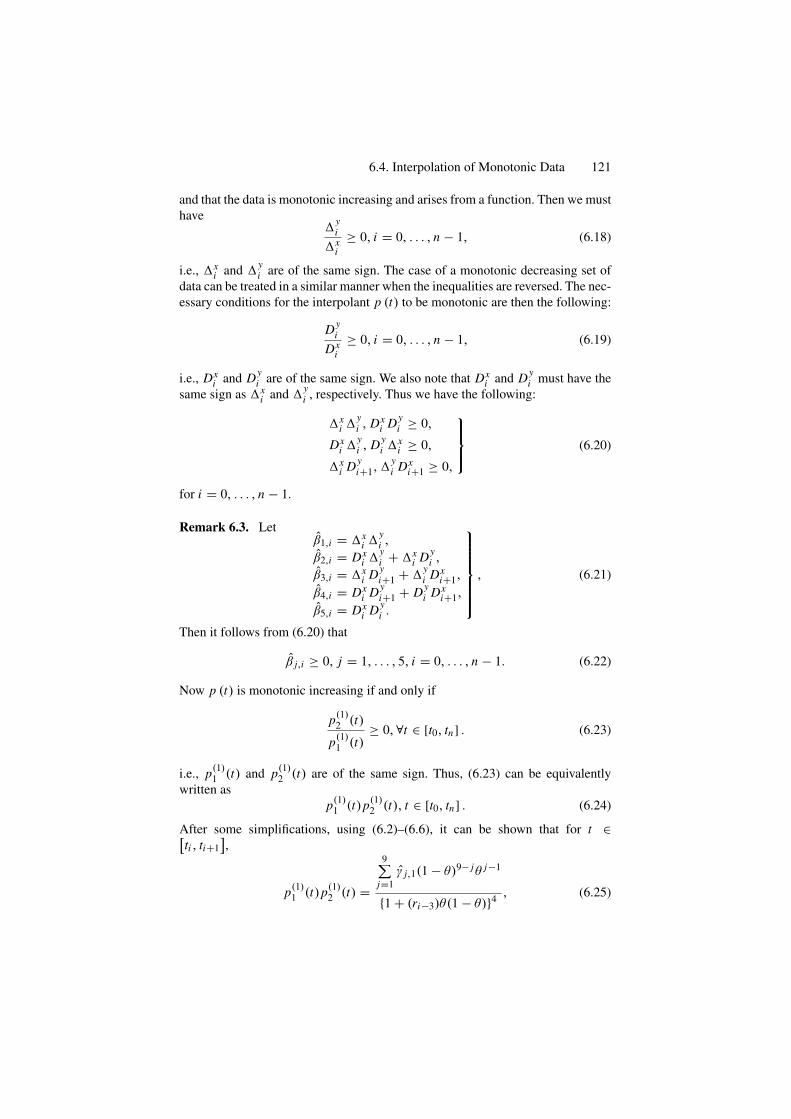
6.4. Interpolation of Monotonic Data 121
and that the data is monotonic increasing and arises from a function. Then we musthave
�yi
�xi
≥ 0, i = 0, . . . , n − 1, (6.18)
i.e., �xi and �
yi are of the same sign. The case of a monotonic decreasing set of
data can be treated in a similar manner when the inequalities are reversed. The nec-essary conditions for the interpolant p (t) to be monotonic are then the following:
Dyi
Dxi
≥ 0, i = 0, . . . , n − 1, (6.19)
i.e., Dxi and Dy
i are of the same sign. We also note that Dxi and Dy
i must have thesame sign as �x
i and �yi , respectively. Thus we have the following:
�xi �
yi , Dx
i Dyi ≥ 0,
Dxi �
yi , Dy
i �xi ≥ 0,
�xi Dy
i+1,�yi Dx
i+1 ≥ 0,
⎫⎪⎬
⎪⎭(6.20)
for i = 0, . . . , n − 1.
Remark 6.3. Letβ1,i = �x
i �yi ,
β2,i = Dxi �
yi + �x
i Dyi ,
β3,i = �xi Dy
i+1 + �yi Dx
i+1,
β4,i = Dxi Dy
i+1 + Dyi Dx
i+1,
β5,i = Dxi Dy
i .
⎫⎪⎪⎪⎪⎪⎬
⎪⎪⎪⎪⎪⎭
, (6.21)
Then it follows from (6.20) that
β j,i ≥ 0, j = 1, . . . , 5, i = 0, . . . , n − 1. (6.22)
Now p (t) is monotonic increasing if and only if
p(1)2 (t)
p(1)1 (t)
≥ 0,∀t ∈ [t0, tn] . (6.23)
i.e., p(1)1 (t) and p(1)
2 (t) are of the same sign. Thus, (6.23) can be equivalentlywritten as
p(1)1 (t)p(1)
2 (t), t ∈ [t0, tn] . (6.24)
After some simplifications, using (6.2)–(6.6), it can be shown that for t ∈[ti , ti+1
],
p(1)1 (t)p(1)
2 (t) =
9∑
j=1γ j,1(1 − θ)9− jθ j−1
{1 + (ri−3)θ(1 − θ)}4 , (6.25)
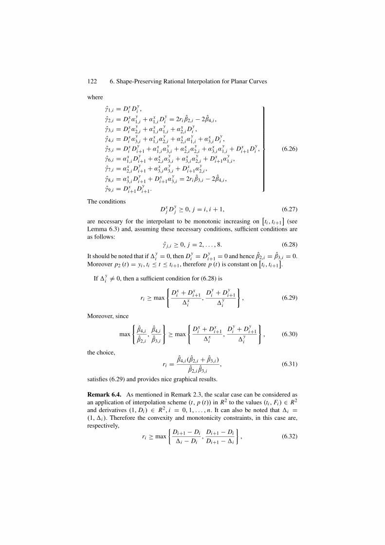
122 6. Shape-Preserving Rational Interpolation for Planar Curves
where
γ1,i = Dxi Dy
i ,
γ2,i = Dxi α
y1,i + αx
1,i Dyi = 2ri β2,i − 2β4,i ,
γ3,i = Dxi α
y2,i + αx
1,iαy1,i + αx
2,i Dyi ,
γ4,i = Dxi α
y3,i + αx
1,iαy2,i + αx
2,iαy1,i + αx
3,i Dyi ,
γ5,i = Dxi Dy
i+1 + αx1,iα
y3,i + αx
2,iαy2,i + αx
3,iαy1,i + Dx
i+1 Dyi ,
γ6,i = αx1,i Dy
i+1 + αx2,iα
y3,i + αx
3,iαy2,i + Dx
i+1αy1,i ,
γ7,i = αx2,i Dy
i+1 + αx3,iα
y3,i + Dx
i+1αy2,i ,
γ8,i = αx3,i Dy
i+1 + Dxi+1α
y3,i = 2ri β3,i − 2β4,i ,
γ9,i = Dxi+1 Dy
i+1.
⎫⎪⎪⎪⎪⎪⎪⎪⎪⎪⎪⎪⎪⎪⎪⎪⎪⎬
⎪⎪⎪⎪⎪⎪⎪⎪⎪⎪⎪⎪⎪⎪⎪⎪⎭
(6.26)
The conditionsDx
j Dyj ≥ 0, j = i, i + 1, (6.27)
are necessary for the interpolant to be monotonic increasing on[ti , ti+1
](see
Lemma 6.3) and, assuming these necessary conditions, sufficient conditions areas follows:
γ j,i ≥ 0, j = 2, . . . , 8. (6.28)
It should be noted that if �yi = 0, then Dy
i = Dyi+1 = 0 and hence β2,i = β3,i = 0.
Moreover p2 (t) = yi , ti ≤ t ≤ ti+1, therefore p (t) is constant on[ti , ti+1
].
If �yi = 0, then a sufficient condition for (6.28) is
ri ≥ max
{Dx
i + Dxi+1
�xi
,Dy
i + Dyi+1
�yi
}
, (6.29)
Moreover, since
max
{β4,i
β2,i,β4,i
β3,i
}
≥ max
{Dx
i + Dxi+1
�xi
,Dy
i + Dyi+1
�yi
}
, (6.30)
the choice,
ri = β4,i (β2,i + β3,i )
β2,i β3,i, (6.31)
satisfies (6.29) and provides nice graphical results.
Remark 6.4. As mentioned in Remark 2.3, the scalar case can be considered asan application of interpolation scheme (t, p (t)) in R2 to the values (ti , Fi ) ∈ R2
and derivatives (1, Di ) ∈ R2, i = 0, 1, . . . , n. It can also be noted that �i =(1,�i ). Therefore the convexity and monotonicity constraints, in this case are,respectively,
ri ≥ max{
Di+1 − Di
�i − Di,
Di+1 − Di
Di+1 − �i
}, (6.32)
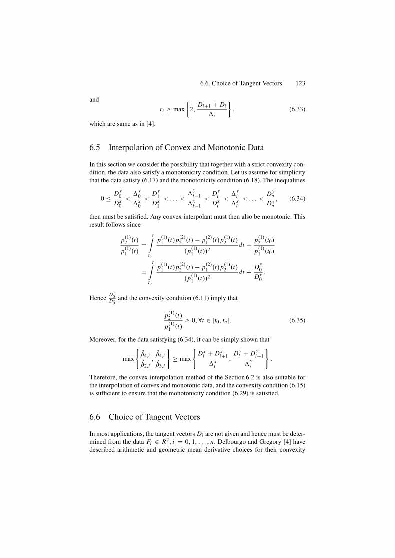
6.6. Choice of Tangent Vectors 123
andri ≥ max
{2,
Di+1 + Di
�i
}, (6.33)
which are same as in [4].
6.5 Interpolation of Convex and Monotonic Data
In this section we consider the possibility that together with a strict convexity con-dition, the data also satisfy a monotonicity condition. Let us assume for simplicitythat the data satisfy (6.17) and the monotonicity condition (6.18). The inequalities
0 ≤ Dy0
Dx0
<�
y0
�x0
<Dy
1Dx
1< . . . <
�yi−1
�xi−1
<Dy
iDx
i<
�yi
�xi
< . . . <Dy
n
Dxn, (6.34)
then must be satisfied. Any convex interpolant must then also be monotonic. Thisresult follows since
p(1)2 (t)
p(1)1 (t)
=t∫
to
p(1)1 (t)p(2)
2 (t) − p(2)1 (t)p(1)
2 (t)
(p(1)1 (t))2
dt + p(1)2 (t0)
p(1)1 (t0)
=t∫
to
p(1)1 (t)p(2)
2 (t) − p(2)1 (t)p(1)
2 (t)
(p(1)1 (t))2
dt + Dy0
Dx0.
Hence Dy0
Dx0
and the convexity condition (6.11) imply that
p(1)2 (t)
p(1)1 (t)
≥ 0,∀t ∈ [t0, tn]. (6.35)
Moreover, for the data satisfying (6.34), it can be simply shown that
max
{β4,i
β2,i,β4,i
β3,i
}
≥ max
{Dx
i + Dxi+1
�xi
,Dy
i + Dyi+1
�yi
}
.
Therefore, the convex interpolation method of the Section 6.2 is also suitable forthe interpolation of convex and monotonic data, and the convexity condition (6.15)is sufficient to ensure that the monotonicity condition (6.29) is satisfied.
6.6 Choice of Tangent Vectors
In most applications, the tangent vectors Di are not given and hence must be deter-mined from the data Fi ∈ R2, i = 0, 1, . . . , n. Delbourgo and Gregory [4] havedescribed arithmetic and geometric mean derivative choices for their convexity
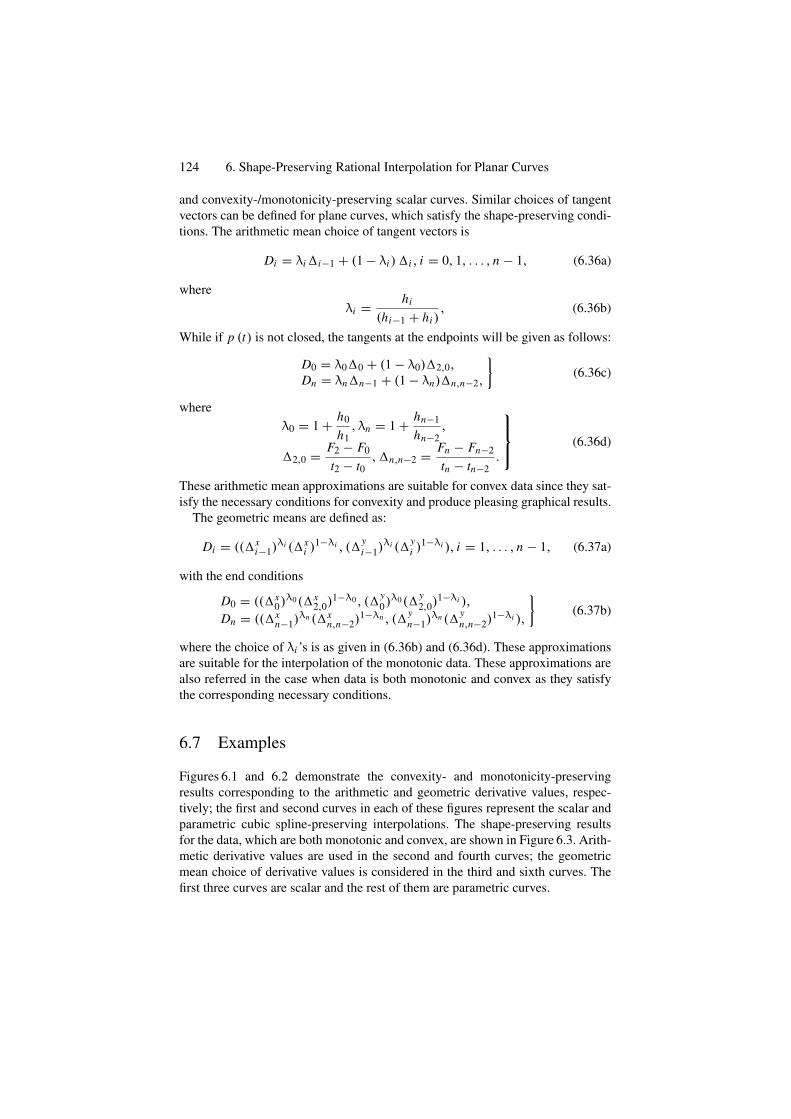
124 6. Shape-Preserving Rational Interpolation for Planar Curves
and convexity-/monotonicity-preserving scalar curves. Similar choices of tangentvectors can be defined for plane curves, which satisfy the shape-preserving condi-tions. The arithmetic mean choice of tangent vectors is
Di = λi�i−1 + (1 − λi )�i , i = 0, 1, . . . , n − 1, (6.36a)
whereλi = hi
(hi−1 + hi ), (6.36b)
While if p (t) is not closed, the tangents at the endpoints will be given as follows:
D0 = λ0�0 + (1 − λ0)�2,0,Dn = λn�n−1 + (1 − λn)�n,n−2,
}(6.36c)
whereλ0 = 1 + h0
h1, λn = 1 + hn−1
hn−2,
�2,0 = F2 − F0
t2 − t0,�n,n−2 = Fn − Fn−2
tn − tn−2.
⎫⎪⎬
⎪⎭(6.36d)
These arithmetic mean approximations are suitable for convex data since they sat-isfy the necessary conditions for convexity and produce pleasing graphical results.
The geometric means are defined as:
Di = ((�xi−1)
λi (�xi )1−λi , (�
yi−1)
λi (�yi )1−λi ), i = 1, . . . , n − 1, (6.37a)
with the end conditions
D0 = ((�x0)λ0(�x
2,0)1−λ0 , (�
y0)λ0(�
y2,0)
1−λi ),
Dn = ((�xn−1)
λn (�xn,n−2)
1−λn , (�yn−1)
λn (�yn,n−2)
1−λi ),
}(6.37b)
where the choice of λi ’s is as given in (6.36b) and (6.36d). These approximationsare suitable for the interpolation of the monotonic data. These approximations arealso referred in the case when data is both monotonic and convex as they satisfythe corresponding necessary conditions.
6.7 Examples
Figures 6.1 and 6.2 demonstrate the convexity- and monotonicity-preservingresults corresponding to the arithmetic and geometric derivative values, respec-tively; the first and second curves in each of these figures represent the scalar andparametric cubic spline-preserving interpolations. The shape-preserving resultsfor the data, which are both monotonic and convex, are shown in Figure 6.3. Arith-metic derivative values are used in the second and fourth curves; the geometricmean choice of derivative values is considered in the third and sixth curves. Thefirst three curves are scalar and the rest of them are parametric curves.
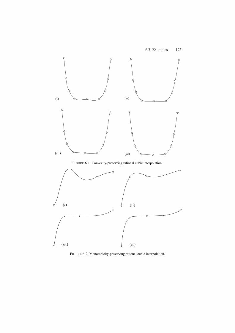
6.7. Examples 125
(iv)(iii)
(i) (ii)
FIGURE 6.1. Convexity-preserving rational cubic interpolation.
(i)
(iii)
(ii)
(iv)
FIGURE 6.2. Monotonicity-preserving rational cubic interpolation.
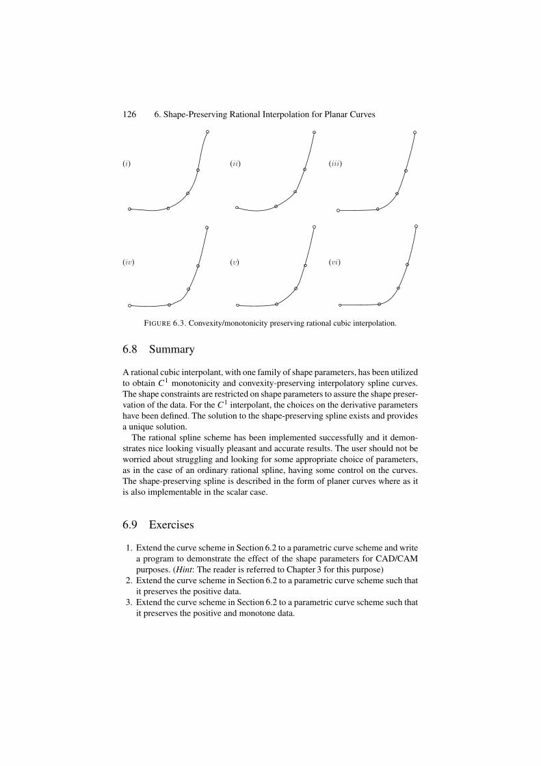
126 6. Shape-Preserving Rational Interpolation for Planar Curves
(i) (ii) (iii)
(iv) (v) (vi)
FIGURE 6.3. Convexity/monotonicity preserving rational cubic interpolation.
6.8 Summary
A rational cubic interpolant, with one family of shape parameters, has been utilizedto obtain C1 monotonicity and convexity-preserving interpolatory spline curves.The shape constraints are restricted on shape parameters to assure the shape preser-vation of the data. For the C1 interpolant, the choices on the derivative parametershave been defined. The solution to the shape-preserving spline exists and providesa unique solution.
The rational spline scheme has been implemented successfully and it demon-strates nice looking visually pleasant and accurate results. The user should not beworried about struggling and looking for some appropriate choice of parameters,as in the case of an ordinary rational spline, having some control on the curves.The shape-preserving spline is described in the form of planer curves where as itis also implementable in the scalar case.
6.9 Exercises
1. Extend the curve scheme in Section 6.2 to a parametric curve scheme and writea program to demonstrate the effect of the shape parameters for CAD/CAMpurposes. (Hint: The reader is referred to Chapter 3 for this purpose)
2. Extend the curve scheme in Section 6.2 to a parametric curve scheme such thatit preserves the positive data.
3. Extend the curve scheme in Section 6.2 to a parametric curve scheme such thatit preserves the positive and monotone data.
References 127
4. Extend the curve scheme in Section 6.2 to a parametric curve scheme such thatit preserves the positive and convex data.
5. Extend the curve scheme in Section 6.2 to a parametric curve scheme such thatit preserves the positive, monotone and convex data.
6. Write programs to visualize the results of the schemes in Exercises 6.9.1–6.9.5.7. Extend the curve scheme in Section 6.2 to a C2 curve scheme.8. Extend the curve scheme in Section 6.3 to a C2 curve scheme.9. Extend the curve scheme in Section 6.4 to a C2 curve scheme.
10. Extend the curve scheme in Section 6.5 to a C2 curve scheme.
References1. McAllister, D.F. and Roulier, J.A. (1981), An algorithm for computing a shape-
preserving osculatory quadratic spline, ACM Trans Math Software 7, 331–347.2. Passow, E., and Roulier, J.A. (1977), Monotone and convex spline interpolation. SIAM
J Num Anal 14, 904–909.3. Fritsch, F.N., and Carlson, R.E. (1980), Monotone piecewise cubic interpolation, SIAM
J Num Anal 17, 238–246.4. Gregory, J.A. (1986), Shape-preserving spline interpolation, Computer-Aided Design,
18(1), 53–57.5. Fritsch, F.N., and Butland, J. (1984), A method for constructing local monotone piece-
wise cubic interpolants, SIAM J Sc Stat Comput 5, 303–304.6. Schumaker, L.L. (1983), On shape-preserving quadratic spline interpolation, SIAM J
Num Anal 20, 854–864.7. Brodlie, K.W., and Butt, S. (1991), Preserving convexity using piecewise cubic inter-
polation, Comput Graphics 15, 15–23.8. Butt, S., and Brodlie, K.W. (1993), Preserving positivity using piecewise cubic inter-
polation, Comput Graphics 17(1), 55–64.9. Sarfraz, M. (1992), Convexity preserving piecewise rational interpolation for planar
curves, Bull Korean Math Soc 29(2), 193–200.10. Sarfraz, M. (1997), Preserving monotone shape of the data using piecewise rational
cubic functions, Comput Graphics 21(1), 5–14.11. Brodlie, K.W. (1985), Methods for drawing curves. In: Fundamental Algorithm for
Computer Graphics, ed. R.A. Earnshaw, Springer-Verlag, Berlin, pp. 303–323.12. DeVore, A., and Yan, Z. (1986), Error analysis for piecewise quadratic curve fitting
algorithms, Comp Aided Geom Design 3, 205–215.13. Greiner, K. (1991), A survey on univariate data interpolation and approximation by
splines of given shape, Math Comp Mod 15, 97–l06.14. Constantini, P. (1997), boundary-valued shape preserving interpolating splines, ACM
Transactions on Mathematical Software, 23(2), 229–251.15. Lahtinen, A. (1996), Monotone interpolation with application to estimation of taper
curves, Ann Numer Math 3, 151–161.16. Sarfraz, M. (1992), Interpolatory rational cubic spline with biased, point and interval
tension, ComputGraphics, 16(4), 427–430.17. Moreton, H.P., and Sequin, C.H. (1995), Minimum Variation Curves and Surfaces
for Computer-Aided Geometric Design, Designing Fair Curves and Surfaces, NickSapidis, ed., Proceedings of SIAM’94 Conference, pp, 123–159.

128 6. Shape-Preserving Rational Interpolation for Planar Curves
18. Sarfraz, M., Butt, S., and Hussain, M. Z. (2001), Visualization of shaped data by arational cubic spline interpolation, Int J Comput Graphics, Elsevier Science, 25(5),833–845.
19. Sarfraz, M. (2000), A rational cubic spline for the visualization of monotonic data,Comput Graphics 24(4), 509–516.
20. Sarfraz, M., and Hussain, M.Z. (2006), Data visualization using rational spline inter-polation, Int J Computational Appl Math, Elsevier Science, 189(1–2), 513–525.
21. Sarfraz, M., Hussain, M.Z., and Chaudhry, F.S. (2005), shape-preserving cubic splinefor data visualization, Int J Comput Graphics CAD/CAM, International Scientific, 1(6),185–194.
22. Sarfraz, M. (2002), Visualization of positive and convex data by a rational cubic spline,Int J Information Sci, Elsevier Science, 146(1–4), 239–254.
23. Sarfraz, M. (2002), Modelling for the visualization of monotone data, Int J ModellingSimulation, ACTA Press, 22(3), 176–185.
7Visualization of Shaped Databy a Rational Cubic Spline
Abstract. A smooth curve interpolation scheme for positive, monotonic and convex data isdescribed. This scheme uses piecewise rational cubic functions. The two families of para-meters, in the description of the rational interpolant have been constrained to preserve theshape of the data. The rational spline scheme has a unique representation. In addition topreserving the shape of positive, monotonic and convex data sets, it also possesses extrafeatures to modify the shape of the design curve when desired. The degree of smoothnessattained is C1.
7.1 Introduction
Smooth curve representation, to visualize the scientific data, is of great sig-nificance in the area of computer graphics and in particular data visualization.Particularly, when the data is obtained from some complex function or from somescientific phenomena, it becomes crucial to incorporate the inherited features ofthe data. Moreover, smoothness is also one of the very important requirementsfor a pleasing visual display. Ordinary spline schemes, although smoother, arenot helpful for the interpolation of the shaped data. Extremely misguided results,violating the inherited features of the data, can be seen when undesired oscilla-tions occur. For example, for the positive data set in Table 7.1, the correspondingcurve in Figure 7.1 is not as may be desired by the user for a positive data. Theuser would be interested in visualizing it as it is displayed in Figure 7.2. Thus,unwanted oscillations that completely destroy the data features need to be con-trolled. Another example is the monotonically increasing data set in Table 7.2. Thecorresponding traditional spline curve is shown in Figure 7.3, which has destroyedthe features of monotonicity as may be desired corresponding to Figure 7.4. Simi-larly, a traditional spline curve in Figure 7.13 is not displaying the convex data inTable 7.10 such that the curve is also convex.
Interpolation is a fundamental process in scientific visualization. Smooth curverepresentation, to visualize the scientific data, is of great significance in variousareas of scientific research including scientific visualization, computer graphics,
129
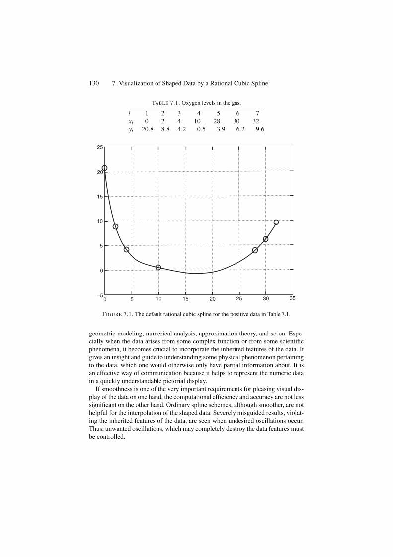
130 7. Visualization of Shaped Data by a Rational Cubic Spline
TABLE 7.1. Oxygen levels in the gas.
i 1 2 3 4 5 6 7xi 0 2 4 10 28 30 32yi 20.8 8.8 4.2 0.5 3.9 6.2 9.6
20
25
10
5
0
−50 5 10 20 25 30 3515
15
FIGURE 7.1. The default rational cubic spline for the positive data in Table 7.1.
geometric modeling, numerical analysis, approximation theory, and so on. Espe-cially when the data arises from some complex function or from some scientificphenomena, it becomes crucial to incorporate the inherited features of the data. Itgives an insight and guide to understanding some physical phenomenon pertainingto the data, which one would otherwise only have partial information about. It isan effective way of communication because it helps to represent the numeric datain a quickly understandable pictorial display.
If smoothness is one of the very important requirements for pleasing visual dis-play of the data on one hand, the computational efficiency and accuracy are not lesssignificant on the other hand. Ordinary spline schemes, although smoother, are nothelpful for the interpolation of the shaped data. Severely misguided results, violat-ing the inherited features of the data, are seen when undesired oscillations occur.Thus, unwanted oscillations, which may completely destroy the data features mustbe controlled.
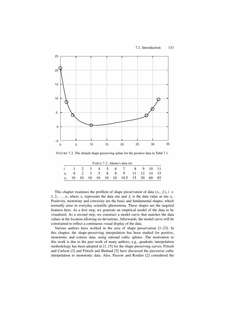
7.1. Introduction 131
20
25
10
5
0
−50 5 10 20 25 30 3515
15
FIGURE 7.2. The default shape-preserving spline for the positive data in Table 7.1.
TABLE 7.2. Akima’s data set.
i 1 2 3 4 5 6 7 8 9 10 11xi 0 2 3 5 6 8 9 11 12 14 15yi 10 10 10 10 10 10 10.5 15 30 60 85
This chapter examines the problem of shape preservation of data (xi , fi ), i =1, 2, . . . , n, where xi represents the data site and fi is the data value at site xi .Positivity, monotony and convexity are the basic and fundamental shapes, whichnormally arise in everyday scientific phenomena. These shapes are the targetedfeatures here. As a first step, we generate an empirical model of the data to bevisualized. As a second step, we construct a model curve that matches the datavalues at the location allowing no deviations. Afterwards, the model curve will beconstrained to reflect a continuous visual display of the data.
Various authors have worked in the area of shape preservation [1–23]. Inthis chapter, the shape-preserving interpolation has been studied for positive,monotonic and convex data, using rational cubic splines. The motivation tothis work is due to the past work of many authors, e.g., quadratic interpolationmethodology has been adopted in [1, 15] for the shape-preserving curves. Fritschand Carlson [3] and Fritsch and Butland [5] have discussed the piecewise cubicinterpolation to monotonic data. Also, Passow and Roulier [2] considered the
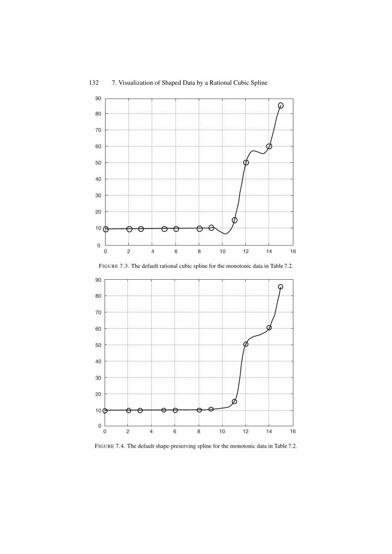
132 7. Visualization of Shaped Data by a Rational Cubic Spline
20
30
40
50
60
70
80
90
10
00
2 4 6 8 10 12 14 16
FIGURE 7.3. The default rational cubic spline for the monotonic data in Table 7.2.
90
80
70
60
50
40
30
20
10
00 2 4 6 8 10 12 14 16
FIGURE 7.4. The default shape-preserving spline for the monotonic data in Table 7.2.
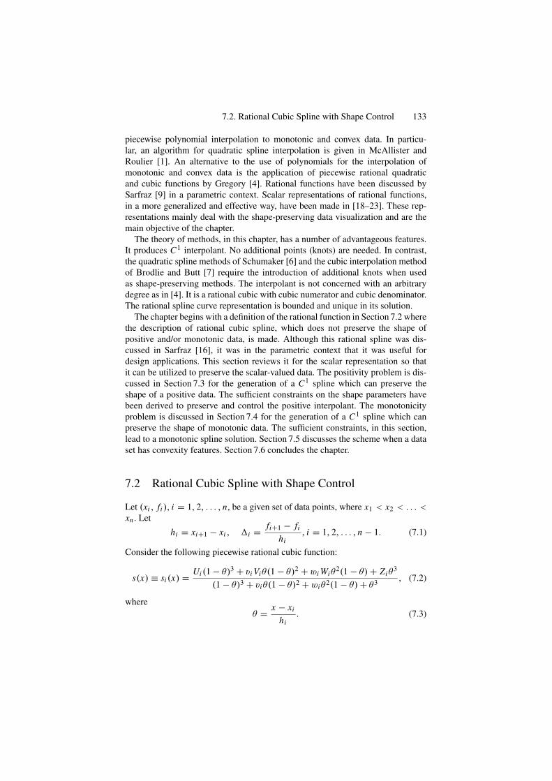
7.2. Rational Cubic Spline with Shape Control 133
piecewise polynomial interpolation to monotonic and convex data. In particu-lar, an algorithm for quadratic spline interpolation is given in McAllister andRoulier [1]. An alternative to the use of polynomials for the interpolation ofmonotonic and convex data is the application of piecewise rational quadraticand cubic functions by Gregory [4]. Rational functions have been discussed bySarfraz [9] in a parametric context. Scalar representations of rational functions,in a more generalized and effective way, have been made in [18–23]. These rep-resentations mainly deal with the shape-preserving data visualization and are themain objective of the chapter.
The theory of methods, in this chapter, has a number of advantageous features.It produces C1 interpolant. No additional points (knots) are needed. In contrast,the quadratic spline methods of Schumaker [6] and the cubic interpolation methodof Brodlie and Butt [7] require the introduction of additional knots when usedas shape-preserving methods. The interpolant is not concerned with an arbitrarydegree as in [4]. It is a rational cubic with cubic numerator and cubic denominator.The rational spline curve representation is bounded and unique in its solution.
The chapter begins with a definition of the rational function in Section 7.2 wherethe description of rational cubic spline, which does not preserve the shape ofpositive and/or monotonic data, is made. Although this rational spline was dis-cussed in Sarfraz [16], it was in the parametric context that it was useful fordesign applications. This section reviews it for the scalar representation so thatit can be utilized to preserve the scalar-valued data. The positivity problem is dis-cussed in Section 7.3 for the generation of a C1 spline which can preserve theshape of a positive data. The sufficient constraints on the shape parameters havebeen derived to preserve and control the positive interpolant. The monotonicityproblem is discussed in Section 7.4 for the generation of a C1 spline which canpreserve the shape of monotonic data. The sufficient constraints, in this section,lead to a monotonic spline solution. Section 7.5 discusses the scheme when a dataset has convexity features. Section 7.6 concludes the chapter.
7.2 Rational Cubic Spline with Shape Control
Let (xi , fi ), i = 1, 2, . . . , n, be a given set of data points, where x1 < x2 < . . . <xn . Let
hi = xi+1 − xi , �i = fi+1 − fi
hi, i = 1, 2, . . . , n − 1. (7.1)
Consider the following piecewise rational cubic function:
s(x) ≡ si (x) = Ui (1 − θ)3 + vi Viθ(1 − θ)2 + wi Wiθ2(1 − θ) + Ziθ
3
(1 − θ)3 + viθ(1 − θ)2 + wiθ2(1 − θ) + θ3 , (7.2)
whereθ = x − xi
hi. (7.3)
134 7. Visualization of Shaped Data by a Rational Cubic Spline
To make the rational function (7.2) C1, one needs to impose the following inter-polatory properties:
s(xi ) = fi , s(xi+1) = fi+1s(1)(xi ) = di , s(1)(xi+1) = di+1
}, (7.4)
which provide the following manipulations:
Ui = fi , Zi = fi+1
Vi = fi + hi di
vi, Wi = fi+1 − hi di+1
wi
⎫⎬
⎭, (7.5)
where s(1) denotes derivative with respect to x and di denotes derivative valuegiven at the knot xi . This leads the piecewise rational cubic (7.2) to the followingpiecewise Hermite interpolant s ∈ C1[x1, xn]:
s(x) ≡ si (x) = Pi (θ)
Qi (θ), (7.6)
where
Pi (θ) = fi (1 − θ)3 + vi Viθ(1 − θ)2 + wi Wiθ2(1 − θ) + fi+1θ
3,
Qi (θ) = (1 − θ)3 + viθ(1 − θ)2 + wiθ2(1 − θ) + θ3.
The parameters vi ’s, wi ’s, and the derivatives di ’s are to be chosen such that themonotonic shape is preserved by the interpolant (7.6). One can note that whenvi = wi = 3, the rational function obviously becomes the standard cubic Hermitepolynomial. Variation for the values of vi ’s and wi ’s control (tighten or loosen) thecurve in different pieces of the curve. This behavior can be seen in the followingsubsection.
7.2.1 Shape Control AnalysisThe parameters vi ’s and wi ’s can be utilized properly to modify the shape of thecurve according to the desire of the user. Their effectiveness, for the shape controlat knot points, can be seen that if vi , wi−1 → ∞, then the curve is pulled towardthe point (xi , fi ) in the neighborhood of the knot position xi . This shape behaviorcan be observed by looking at si (x) in Equation (7.6). This form is similar to thatof a Bernstein-Bezier formulation. One can observe that when vi , wi−1 → ∞,then Vi and Wi−1 → fi .
The interval shape control behavior can be observed by rewriting si (x) in Equa-tion (7.6) to the following simplified form:
s(x) = fi (1 − θ) + fi+1θ
+[(1− θ)(di − �i ) + θ(�i − di+1) + θ(1− θ)�i (wi − vi )
]hiθ(1− θ)
Qi (θ).
(7.7)
7.2. Rational Cubic Spline with Shape Control 135
When both vi and wi → ∞, it is simple to see the convergence to the followinglinear interpolant:
s(x) = fi (1 − θ) + fi+1θ. (7.8)
It should be noted that the shape control analysis is valid only if the bounded deriv-ative values are assumed. A description of appropriate choices for such derivativevalues is made in the following subsection.
7.2.2 Determination of DerivativesIn most applications, the derivative parameters {di } are not given and hence mustbe determined either from the given data (xi , fi ), i = 1, 2, . . . , n, or by someother means. In this article, they are computed from the given data in such a waythat the C1 smoothness of the interpolant (7.6) is maintained. These methods arethe approximations based on various mathematical theories. The descriptions ofsuch approximations are as follows:
7.2.2.1 Derivative Method I
The arithmetic mean method is the three-point difference approximation methodbased on arithmetic manipulation. It is defined as follows:
di ={
0, if �i−1 = 0 or �i = 0,(hi�i−1 + hi−1�i ) / (hi + hi−1) , otherwise, i = 2, 3, . . . , n − 1.
(7.9)The end conditions are given as:
d1 ={
0, if �1 = 0 or sgn(d∗
1) = sgn (�1) ,
d∗1 = �1 + (�1 − �2) h1/ (h1 + h2) , otherwise. (7.10)
dn ={
0, if �n−1 = 0 or sgn(d∗
n) = sgn (�n−1) ,
d∗n = �n−1 + (�n−1 − �n−2) hn−1/ (hn−1 + hn−2) , otherwise.
(7.11)
7.2.2.2 Derivative Method II
The geometric mean method provides the non-linear approximations which aredefined as follows:
di ={
0, if �i−1 = 0 or �i = 0,
�hi /(hi−1+hi)i−1 �
hi−1/(hi−1+hi)i otherwise, i = 2, 3, . . . . . . ., n − 1.
(7.12)The end conditions are given as:
di ={
0, if�1 = 0 or �3,1 = 0�1{�1/�3,1
}h1/h2 , otherwise.(7.13)
di ={
0, if �n−1 = 0 or �n,n−2 = 0�n−1
{�n−1/�n,n−2
}hn−1/hn−2 , otherwise.(7.14)
136 7. Visualization of Shaped Data by a Rational Cubic Spline
where�3,1 = ( f3 − f1) / (x3 − x1) ,
�n,n−2 = ( fn − fn−2) / (xn − xn−2) .
}(7.15)
7.2.2.3 Derivative Method III
Another nonlinear choice of derivative values is the following:
di ={
0 if fi+1 − fi−1 = 0,
�i−1�i/[( fi+1 − fi−1) / (xi+1 − xi−1)
]otherwise, i = 2, 3, . . . , n − 1
with end conditions
d1 ={
0 if f3 − f1 = 0,
�21/�3,1 otherwise,
dn ={
0 if fn − fn−2 = 0,
�2n−1/�n,n−2 otherwise
For given bounded data, the derivative approximations in Subsections 7.2.2.1,7.2.2.2 and 7.2.2.3 are bounded. Hence, for bounded values of the appropriateshape parameters:
vi , wi , i = 1, 2, . . . n − 1, (7.16)
the interpolant is bounded and unique. Therefore, we can conclude the above dis-cussion in the following:
Theorem 7.1. For bounded vi , wi ,∀i , and the derivative approximations in Sub-sections 7.2.2.1, 7.2.2.2 and 7.2.2.3, the spline solution of the interpolant (7.6)exists and is unique.
7.2.3 Examples and DiscussionFor the demonstration of a C1 rational cubic curve scheme, the derivatives arecomputed from the Subsections 7.2.2.1. We choose the following choice of shapeparameters:
vi = 3 = wi , (7.17)
to generate the initial default curves. This initial default curve is actually the sameas a cubic spline curve. Further modification can be made by changing these para-meters interactively.
Figures 7.1 and 7.3 are the default curves for the positive and monotonicallyincreasing data in Table 7.1 and Table 7.2, respectively. The data in Table 7.1 hasbeen taken from an experiment showing oxygen levels in the flue gas (see [7]) andthe data in Table 7.2 is another scientific data (Akima’s data) discussed in [3]. Itcan be seen that the ordinary spline curves do not guarantee to preserve the shapeof the data.
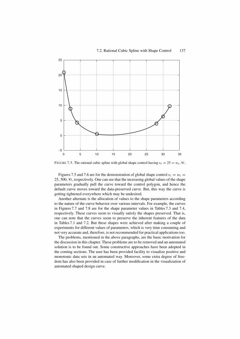
7.2. Rational Cubic Spline with Shape Control 137
25
20
15
10
5
0
−50 5 10 15 20 25 30 35
FIGURE 7.5. The rational cubic spline with global shape control having vi = 25 = wi , ∀i .
Figures 7.5 and 7.6 are for the demonstration of global shape control vi = wi =25, 500,∀i , respectively. One can see that the increasing global values of the shapeparameters gradually pull the curve toward the control polygon, and hence thedefault curve moves toward the data-preserved curve. But, this way the curve isgetting tightened everywhere which may be undesired.
Another alternate is the allocation of values to the shape parameters accordingto the nature of the curve behavior over various intervals. For example, the curvesin Figures 7.7 and 7.8 are for the shape parameter values in Tables 7.3 and 7.4,respectively. These curves seem to visually satisfy the shapes preserved. That is,one can note that the curves seem to preserve the inherent features of the datain Tables 7.1 and 7.2. But these shapes were achieved after making a couple ofexperiments for different values of parameters, which is very time consuming andnot very accurate and, therefore, is not recommended for practical applications too.
The problems, mentioned in the above paragraphs, are the basic motivation forthe discussion in this chapter. These problems are to be removed and an automatedsolution is to be found out. Some constructive approaches have been adopted inthe coming sections. The user has been provided facility to visualize positive andmonotonic data sets in an automated way. Moreover, some extra degree of free-dom has also been provided in case of further modification in the visualization ofautomated shaped design curve.
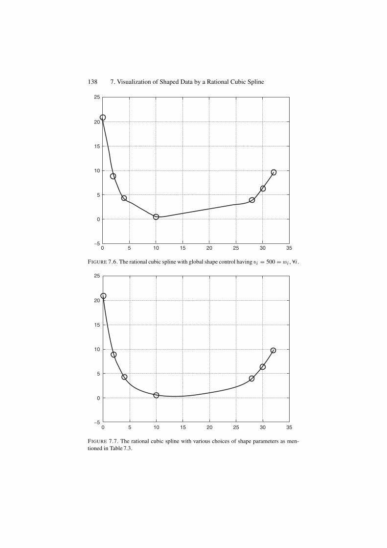
138 7. Visualization of Shaped Data by a Rational Cubic Spline
25
20
15
10
5
0
−50 5 10 15 20 25 30 35
FIGURE 7.6. The rational cubic spline with global shape control having vi = 500 = wi , ∀i .
20
25
15
10
5
0
−50 5 10 15 20 25 30 35
FIGURE 7.7. The rational cubic spline with various choices of shape parameters as men-tioned in Table 7.3.
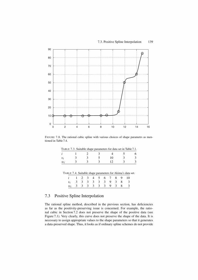
7.3. Positive Spline Interpolation 139
90
80
70
60
50
40
30
20
10
00 2 4 6 8 10 12 14 16
FIGURE 7.8. The rational cubic spline with various choices of shape parametrs as men-tioned in Table 7.4.
TABLE 7.3. Suitable shape parameters for data set in Table 7.1.
i 1 2 3 4 5 6vi 3 3 5 10 3 3wi 3 3 3 12 3 3
TABLE 7.4. Suitable shape parameters for Akima’s data set.
i 1 2 3 4 5 6 7 8 9 10vi 3 3 3 3 3 3 9 3 8 3wi 3 3 3 3 3 3 9 3 8 3
7.3 Positive Spline Interpolation
The rational spline method, described in the previous section, has deficienciesas far as the positivity-preserving issue is concerned. For example, the ratio-nal cubic in Section 7.2 does not preserve the shape of the positive data (seeFigure 7.1). Very clearly, this curve does not preserve the shape of the data. It isnecessary to assign appropriate values to the shape parameters so that it generatesa data-preserved shape. Thus, it looks as if ordinary spline schemes do not provide
140 7. Visualization of Shaped Data by a Rational Cubic Spline
the desired shape features, and hence some further treatment is required to achievea shape-preserving spline for positive data.
One way, for the above spline method, to achieve the positivity preserving inter-polant is to play with shape parameters vi ’s and wi ’s, on trial and error basis, inthose regions of the curve where the shape violations are found. This strategy mayresult in a required display as can be seen in the previous section. But this is not acomfortable and accurate way to manipulate the desired shape preserving curve.
Another way, which is more effective, useful and is the objective of this arti-cle, is the automated generation of positivity-preserving curve. This requires anautomated computation of suitable shape parameters and derivative values. Toproceed with this strategy, some mathematical treatment is required which willbe explained in the following paragraphs.
For simplicity of presentation, let us assume positive set of data:
(x1, f1), (x2, f2), . . . , (xn, fn)
so thatx1 < x2 < . . . < xn, (7.18)
andf1 > 0, f2 > 0, . . . , fn > 0, (7.19)
It is required to develop sufficient conditions on piecewise rational cubics underwhich C1 positive interpolation is preserved. The key idea, to preserve positivityusing s(x), is to assign suitable automated values to vi , wi in each interval.
As vi , wi > 0 guarantee strictly positive denominator Qi (θ), so initial condi-tions on vi , wi are:
vi > 0, wi > 0(vi < 0, wi < 0, for positive data), i = 1, 2, . . . , n − 1. (7.20)
Since Qi (θ) > 0 for all vi , wi > 0, so the positivity of the interpolant (7.6)depends on the positivity of the cubic polynomial Pi (θ). Thus, the problemreduces to the determination of appropriate values of vi , wi for which the polyno-mial Pi (θ) is positive. Now, Pi (θ) can be expressed as follows:
Pi (t) = αiθ3 + βiθ
2 + γiθ + δi , (7.21)
whereαi = (1 − wi ) fi+1 − (1 − vi ) fi + (di+1 + di )hi ,
βi = wi fi+1 − (3 − 2vi ) fi − (di+1 + di )hi ,
γi = di hi − (3 − vi ) fi ,
δi = fi .
⎫⎪⎪⎪⎬
⎪⎪⎪⎭
(7.22)
For the strict inequality (for positive data) in (7.6), according to Butt and Brodlie[8], Pi (θ) > 0 if and only if
(P ′i (0), P ′
i (1)) ∈ R1U R2. (7.23)
7.3. Positive Spline Interpolation 141
where
R1 ={(a, b) : a >
−3 fi
hi, b <
3 fi+1
hi
}, (7.24)
R2 = {(a, b) : 36 fi fi+1(a2 + b2 + ab − 3�i (a + b) + 3�2i )+
3( fi+1a − fi b)(2hi ab − 3 fi+1a + 3 fi b)+4hi ( fi+1a3 − fi b3) − h2
i a2b2 > 0}.
⎫⎬
⎭(7.25)
We have
P ′i (0) = fi
hi(vi − 3) + di ,
P ′i (1) = di+1 − fi+1
hi(wi − 3).
Now (7.23) is true when
(P ′i (0), P ′
i (1)) ∈ R1,
P ′i (0) >
−3 fi
hi, P ′
i (1) <3 fi+1
hi.
This leads to the following constraints:
vi > mi , wi > Mi . (7.26)
wheremi = Max
{0,
−hi di
fi
}, Mi = Max
{0,
hi di+1
fi+1
}. (7.27)
Further(P ′
i (0), P ′i (1)) ∈ R2
if
36 fi fi+1[φ21(ri , ui ) + φ2
2(wi ) + φ1(vi )φ2(wi ) − 3�i (φ1(vi ) + φ2(wi )) + 3�2i ]+
3[ fi+1φ1(vi ) − yi φ2(wi )][2hi φ1(vi )φ2(wi ) − 3 fi+1φ1(vi ) + 3 fi φ2(wi )]+4hi [ fi+1φ3
1(vi ) − yi φ32(wi )] − h2
i φ21(vi )φ
22(wi ) > 0
⎫⎬
⎭
(7.28)where
φ1(vi ) = P ′i (0),
φ2(wi ) = P ′i (1).
}(7.29)
This leads to the following:
Theorem 7.2. For a strictly positive data, the rational cubic interpolant (7.6)preserves positivity if and only if either (7.26) or (7.28) is satisfied.
Remark 7.1. The constraints (7.27) can be further modified to incorporate bothshape-preserving and shape control features. Without loss of generality, one canfind parameters ri and qi satisfying
ri , qi ≥ 1. (7.30)
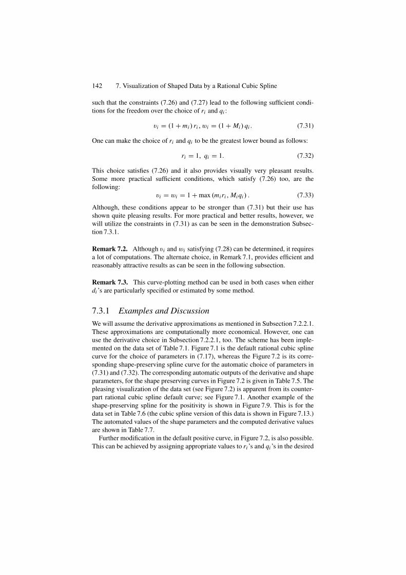
142 7. Visualization of Shaped Data by a Rational Cubic Spline
such that the constraints (7.26) and (7.27) lead to the following sufficient condi-tions for the freedom over the choice of ri and qi :
vi = (1 + mi ) ri , wi = (1 + Mi ) qi . (7.31)
One can make the choice of ri and qi to be the greatest lower bound as follows:
ri = 1, qi = 1. (7.32)
This choice satisfies (7.26) and it also provides visually very pleasant results.Some more practical sufficient conditions, which satisfy (7.26) too, are thefollowing:
vi = wi = 1 + max (miri , Mi qi ) . (7.33)
Although, these conditions appear to be stronger than (7.31) but their use hasshown quite pleasing results. For more practical and better results, however, wewill utilize the constraints in (7.31) as can be seen in the demonstration Subsec-tion 7.3.1.
Remark 7.2. Although vi and wi satisfying (7.28) can be determined, it requiresa lot of computations. The alternate choice, in Remark 7.1, provides efficient andreasonably attractive results as can be seen in the following subsection.
Remark 7.3. This curve-plotting method can be used in both cases when eitherdi ’s are particularly specified or estimated by some method.
7.3.1 Examples and DiscussionWe will assume the derivative approximations as mentioned in Subsection 7.2.2.1.These approximations are computationally more economical. However, one canuse the derivative choice in Subsection 7.2.2.1, too. The scheme has been imple-mented on the data set of Table 7.1. Figure 7.1 is the default rational cubic splinecurve for the choice of parameters in (7.17), whereas the Figure 7.2 is its corre-sponding shape-preserving spline curve for the automatic choice of parameters in(7.31) and (7.32). The corresponding automatic outputs of the derivative and shapeparameters, for the shape preserving curves in Figure 7.2 is given in Table 7.5. Thepleasing visualization of the data set (see Figure 7.2) is apparent from its counter-part rational cubic spline default curve; see Figure 7.1. Another example of theshape-preserving spline for the positivity is shown in Figure 7.9. This is for thedata set in Table 7.6 (the cubic spline version of this data is shown in Figure 7.13.)The automated values of the shape parameters and the computed derivative valuesare shown in Table 7.7.
Further modification in the default positive curve, in Figure 7.2, is also possible.This can be achieved by assigning appropriate values to ri ’s and qi ’s in the desired
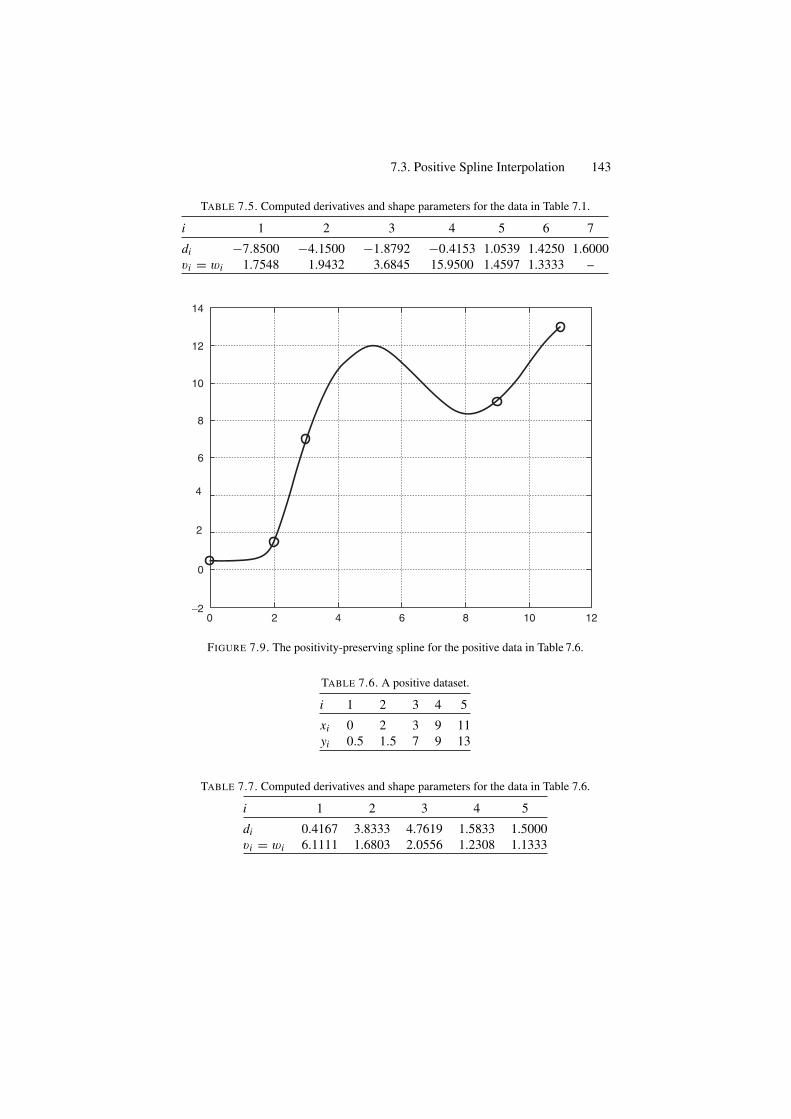
7.3. Positive Spline Interpolation 143
TABLE 7.5. Computed derivatives and shape parameters for the data in Table 7.1.
i 1 2 3 4 5 6 7
di −7.8500 −4.1500 −1.8792 −0.4153 1.0539 1.4250 1.6000vi = wi 1.7548 1.9432 3.6845 15.9500 1.4597 1.3333 –
14
12
10
8
6
4
2
0
−20 2 4 6 8 10 12
FIGURE 7.9. The positivity-preserving spline for the positive data in Table 7.6.
TABLE 7.6. A positive dataset.
i 1 2 3 4 5
xi 0 2 3 9 11yi 0.5 1.5 7 9 13
TABLE 7.7. Computed derivatives and shape parameters for the data in Table 7.6.
i 1 2 3 4 5
di 0.4167 3.8333 4.7619 1.5833 1.5000vi = wi 6.1111 1.6803 2.0556 1.2308 1.1333
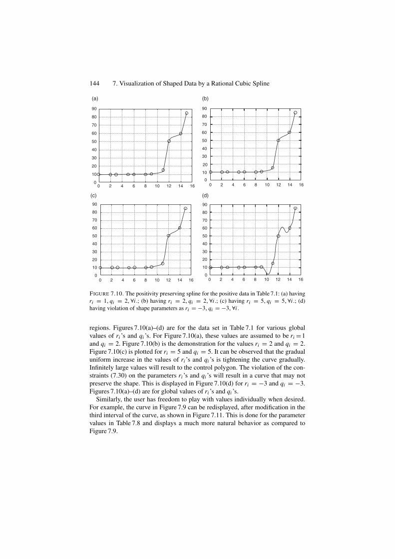
144 7. Visualization of Shaped Data by a Rational Cubic Spline
0 42 6 8 10 12 14 16 0 42 6 8 10 12 14 16
0 42 6 8 10 12 14 160 42 6 8 10 12 14 16
90
80
70
40
30
20
10
0
60
50
90
80
70
40
30
20
10
0
60
50
90
80
70
40
30
20
10
0
60
50
90
80
70
40
30
20
10
0
60
50
(a) (b)
(c) (d)
FIGURE 7.10. The positivity preserving spline for the positive data in Table 7.1: (a) havingri = 1, qi = 2, ∀i .; (b) having ri = 2, qi = 2, ∀i .; (c) having ri = 5, qi = 5,∀i .; (d)having violation of shape parameters as ri = −3, qi = −3, ∀i .
regions. Figures 7.10(a)–(d) are for the data set in Table 7.1 for various globalvalues of ri ’s and qi ’s. For Figure 7.10(a), these values are assumed to be ri =1and qi = 2. Figure 7.10(b) is the demonstration for the values ri = 2 and qi = 2.Figure 7.10(c) is plotted for ri = 5 and qi = 5. It can be observed that the gradualuniform increase in the values of ri ’s and qi ’s is tightening the curve gradually.Infinitely large values will result to the control polygon. The violation of the con-straints (7.30) on the parameters ri ’s and qi ’s will result in a curve that may notpreserve the shape. This is displayed in Figure 7.10(d) for ri = −3 and qi = −3.Figures 7.10(a)–(d) are for global values of ri ’s and qi ’s.
Similarly, the user has freedom to play with values individually when desired.For example, the curve in Figure 7.9 can be redisplayed, after modification in thethird interval of the curve, as shown in Figure 7.11. This is done for the parametervalues in Table 7.8 and displays a much more natural behavior as compared toFigure 7.9.
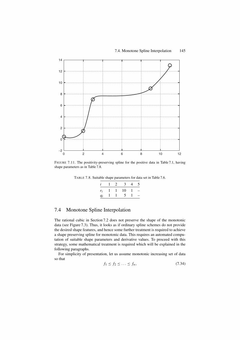
7.4. Monotone Spline Interpolation 145
14
12
10
8
6
4
2
0
−20 2 4 6 8 10 12
FIGURE 7.11. The positivity-preserving spline for the positive data in Table 7.1, havingshape parameters as in Table 7.8.
TABLE 7.8. Suitable shape parameters for data set in Table 7.6.
i 1 2 3 4 5
ri 1 1 10 1 –qi 1 1 5 1 –
7.4 Monotone Spline Interpolation
The rational cubic in Section 7.2 does not preserve the shape of the monotonicdata (see Figure 7.3). Thus, it looks as if ordinary spline schemes do not providethe desired shape features, and hence some further treatment is required to achievea shape preserving spline for monotonic data. This requires an automated compu-tation of suitable shape parameters and derivative values. To proceed with thisstrategy, some mathematical treatment is required which will be explained in thefollowing paragraphs.
For simplicity of presentation, let us assume monotonic increasing set of dataso that
f1 ≤ f2 ≤ . . . ≤ fn, (7.34)
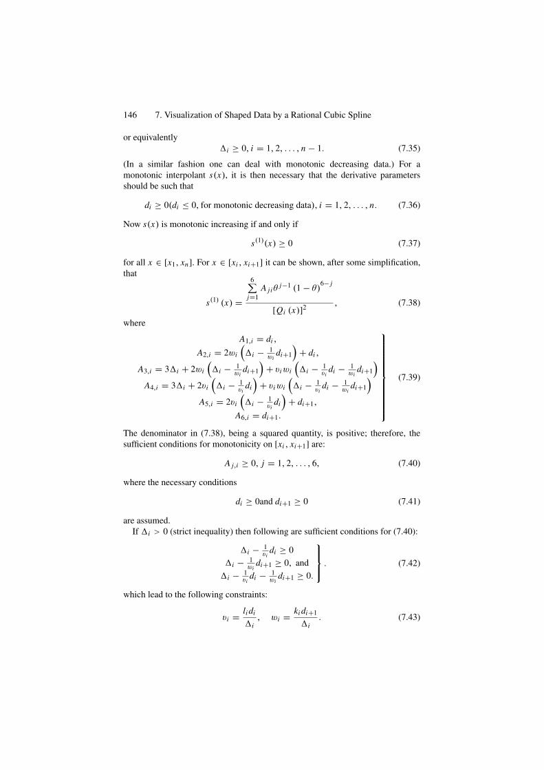
146 7. Visualization of Shaped Data by a Rational Cubic Spline
or equivalently�i ≥ 0, i = 1, 2, . . . , n − 1. (7.35)
(In a similar fashion one can deal with monotonic decreasing data.) For amonotonic interpolant s(x), it is then necessary that the derivative parametersshould be such that
di ≥ 0(di ≤ 0, for monotonic decreasing data), i = 1, 2, . . . , n. (7.36)
Now s(x) is monotonic increasing if and only if
s(1)(x) ≥ 0 (7.37)
for all x ∈ [x1, xn]. For x ∈ [xi , xi+1] it can be shown, after some simplification,that
s(1) (x) =
6∑
j=1A jiθ
j−1 (1 − θ)6− j
[Qi (x)]2 , (7.38)
where
A1,i = di ,
A2,i = 2wi
(�i − 1
widi+1
)+ di ,
A3,i = 3�i + 2wi
(�i − 1
widi+1
)+ viwi
(�i − 1
vidi − 1
widi+1
)
A4,i = 3�i + 2vi
(�i − 1
vidi
)+ viwi
(�i − 1
vidi − 1
widi+1
)
A5,i = 2vi
(�i − 1
vidi
)+ di+1,
A6,i = di+1.
⎫⎪⎪⎪⎪⎪⎪⎪⎪⎪⎪⎬
⎪⎪⎪⎪⎪⎪⎪⎪⎪⎪⎭
(7.39)
The denominator in (7.38), being a squared quantity, is positive; therefore, thesufficient conditions for monotonicity on [xi , xi+1] are:
A j,i ≥ 0, j = 1, 2, . . . , 6, (7.40)
where the necessary conditions
di ≥ 0and di+1 ≥ 0 (7.41)
are assumed.If �i > 0 (strict inequality) then following are sufficient conditions for (7.40):
�i − 1vi
di ≥ 0�i − 1
widi+1 ≥ 0, and
�i − 1vi
di − 1wi
di+1 ≥ 0.
⎫⎪⎬
⎪⎭. (7.42)
which lead to the following constraints:
vi = li di
�i, wi = ki di+1
�i. (7.43)
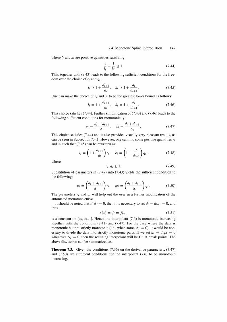
7.4. Monotone Spline Interpolation 147
where li and ki are positive quantities satisfying
1li
+ 1ki
≤ 1. (7.44)
This, together with (7.43) leads to the following sufficient conditions for the free-dom over the choice of ri and qi :
li ≥ 1 + di+1
di, ki ≥ 1 + di
di+1. (7.45)
One can make the choice of ri and qi to be the greatest lower bound as follows:
li = 1 + di+1
di, ki = 1 + di
di+1. (7.46)
This choice satisfies (7.44). Further simplification of (7.43) and (7.46) leads to thefollowing sufficient conditions for monotonicity:
vi = di + di+1
�i, wi = di + di+1
�i. (7.47)
This choice satisfies (7.44) and it also provides visually very pleasant results, ascan be seen in Subsection 7.4.1. However, one can find some positive quantities riand qi such that (7.45) can be rewritten as:
li =(
1 + di+1
di
)ri , ki =
(1 + di
di+1
)qi . (7.48)
whereri , qi ≥ 1. (7.49)
Substitution of parameters in (7.47) into (7.43) yields the sufficient condition tothe following:
vi =(
di + di+1
�i
)ri , wi =
(di + di+1
�i
)qi . (7.50)
The parameters ri and qi will help out the user in a further modification of theautomated monotone curve.
It should be noted that if �i = 0, then it is necessary to set di = di+1 = 0, andthus
s(x) = fi = fi+1 (7.51)
is a constant on [xi , xi+1]. Hence the interpolant (7.6) is monotonic increasingtogether with the conditions (7.41) and (7.47). For the case where the data ismonotonic but not strictly monotonic (i.e., when some �i = 0), it would be nec-essary to divide the data into strictly monotonic parts. If we set di = di+1 = 0whenever �i = 0, then the resulting interpolant will be C0 at break points. Theabove discussion can be summarized as:
Theorem 7.3. Given the conditions (7.36) on the derivative parameters, (7.47)and (7.50) are sufficient conditions for the interpolant (7.6) to be monotonicincreasing.
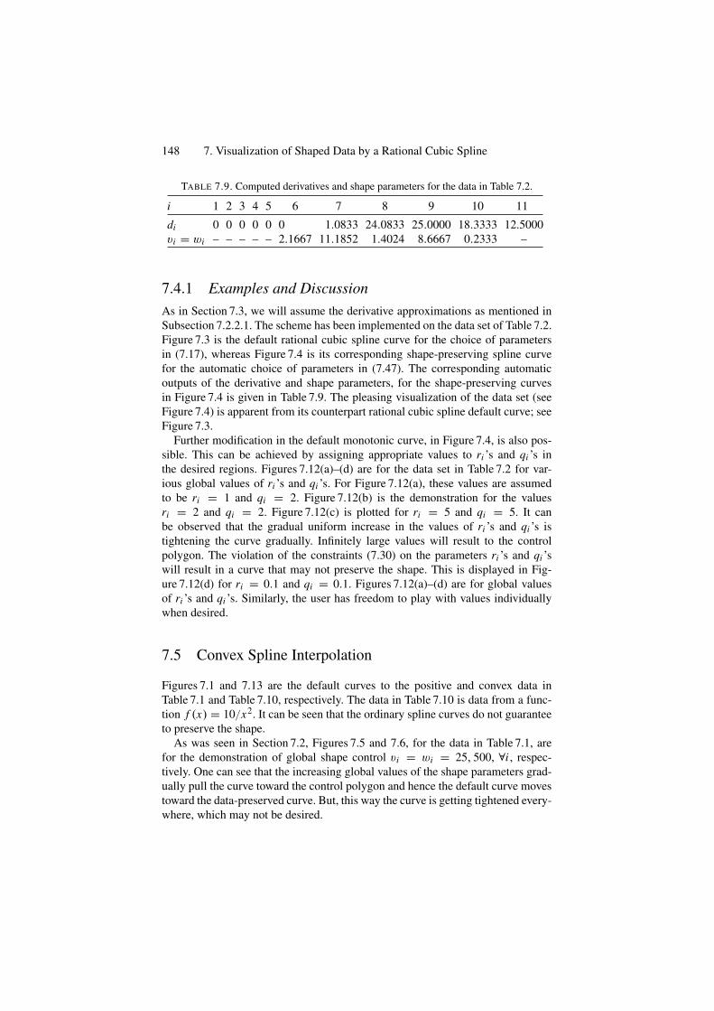
148 7. Visualization of Shaped Data by a Rational Cubic Spline
TABLE 7.9. Computed derivatives and shape parameters for the data in Table 7.2.
i 1 2 3 4 5 6 7 8 9 10 11
di 0 0 0 0 0 0 1.0833 24.0833 25.0000 18.3333 12.5000vi = wi – – – – – 2.1667 11.1852 1.4024 8.6667 0.2333 –
7.4.1 Examples and DiscussionAs in Section 7.3, we will assume the derivative approximations as mentioned inSubsection 7.2.2.1. The scheme has been implemented on the data set of Table 7.2.Figure 7.3 is the default rational cubic spline curve for the choice of parametersin (7.17), whereas Figure 7.4 is its corresponding shape-preserving spline curvefor the automatic choice of parameters in (7.47). The corresponding automaticoutputs of the derivative and shape parameters, for the shape-preserving curvesin Figure 7.4 is given in Table 7.9. The pleasing visualization of the data set (seeFigure 7.4) is apparent from its counterpart rational cubic spline default curve; seeFigure 7.3.
Further modification in the default monotonic curve, in Figure 7.4, is also pos-sible. This can be achieved by assigning appropriate values to ri ’s and qi ’s inthe desired regions. Figures 7.12(a)–(d) are for the data set in Table 7.2 for var-ious global values of ri ’s and qi ’s. For Figure 7.12(a), these values are assumedto be ri = 1 and qi = 2. Figure 7.12(b) is the demonstration for the valuesri = 2 and qi = 2. Figure 7.12(c) is plotted for ri = 5 and qi = 5. It canbe observed that the gradual uniform increase in the values of ri ’s and qi ’s istightening the curve gradually. Infinitely large values will result to the controlpolygon. The violation of the constraints (7.30) on the parameters ri ’s and qi ’swill result in a curve that may not preserve the shape. This is displayed in Fig-ure 7.12(d) for ri = 0.1 and qi = 0.1. Figures 7.12(a)–(d) are for global valuesof ri ’s and qi ’s. Similarly, the user has freedom to play with values individuallywhen desired.
7.5 Convex Spline Interpolation
Figures 7.1 and 7.13 are the default curves to the positive and convex data inTable 7.1 and Table 7.10, respectively. The data in Table 7.10 is data from a func-tion f (x) = 10/x2. It can be seen that the ordinary spline curves do not guaranteeto preserve the shape.
As was seen in Section 7.2, Figures 7.5 and 7.6, for the data in Table 7.1, arefor the demonstration of global shape control vi = wi = 25, 500, ∀i , respec-tively. One can see that the increasing global values of the shape parameters grad-ually pull the curve toward the control polygon and hence the default curve movestoward the data-preserved curve. But, this way the curve is getting tightened every-where, which may not be desired.
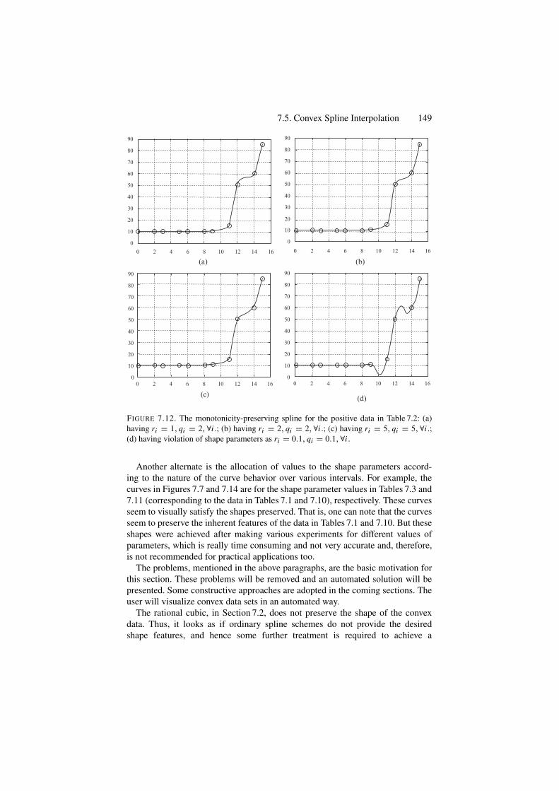
7.5. Convex Spline Interpolation 149
90
80
70
50
60
40
30
20
10
0
90
80
70
50
60
40
30
20
10
0
90
80
70
50
60
40
30
20
10
0
90
80
70
50
60
40
30
20
10
0
0 2 4 6 8 10 12 14 16 0 2 4 6 8 10 12 14 16
0 2 4 6 8 10 12 14 160 2 4 6 8 10 12 14 16
(a) (b)
(c) (d)
FIGURE 7.12. The monotonicity-preserving spline for the positive data in Table 7.2: (a)having ri = 1, qi = 2, ∀i .; (b) having ri = 2, qi = 2, ∀i .; (c) having ri = 5, qi = 5, ∀i .;(d) having violation of shape parameters as ri = 0.1, qi = 0.1, ∀i .
Another alternate is the allocation of values to the shape parameters accord-ing to the nature of the curve behavior over various intervals. For example, thecurves in Figures 7.7 and 7.14 are for the shape parameter values in Tables 7.3 and7.11 (corresponding to the data in Tables 7.1 and 7.10), respectively. These curvesseem to visually satisfy the shapes preserved. That is, one can note that the curvesseem to preserve the inherent features of the data in Tables 7.1 and 7.10. But theseshapes were achieved after making various experiments for different values ofparameters, which is really time consuming and not very accurate and, therefore,is not recommended for practical applications too.
The problems, mentioned in the above paragraphs, are the basic motivation forthis section. These problems will be removed and an automated solution will bepresented. Some constructive approaches are adopted in the coming sections. Theuser will visualize convex data sets in an automated way.
The rational cubic, in Section 7.2, does not preserve the shape of the convexdata. Thus, it looks as if ordinary spline schemes do not provide the desiredshape features, and hence some further treatment is required to achieve a
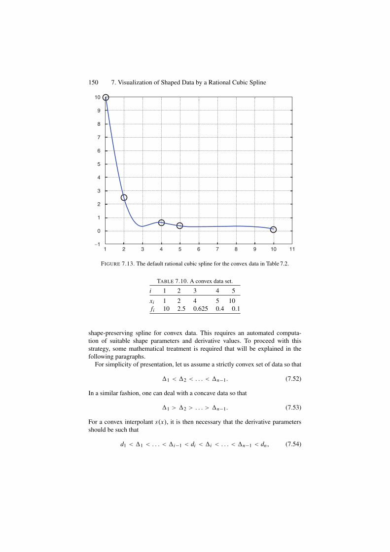
150 7. Visualization of Shaped Data by a Rational Cubic Spline
10
9
8
7
6
5
4
3
2
1
0
−11 2 3 4 5 6 7 8 9 10 11
FIGURE 7.13. The default rational cubic spline for the convex data in Table 7.2.
TABLE 7.10. A convex data set.
i 1 2 3 4 5
xi 1 2 4 5 10fi 10 2.5 0.625 0.4 0.1
shape-preserving spline for convex data. This requires an automated computa-tion of suitable shape parameters and derivative values. To proceed with thisstrategy, some mathematical treatment is required that will be explained in thefollowing paragraphs.
For simplicity of presentation, let us assume a strictly convex set of data so that
�1 < �2 < . . . < �n−1. (7.52)
In a similar fashion, one can deal with a concave data so that
�1 > �2 > . . . > �n−1. (7.53)
For a convex interpolant s(x), it is then necessary that the derivative parametersshould be such that
d1 < �1 < . . . < �i−1 < di < �i < . . . < �n−1 < dn, (7.54)
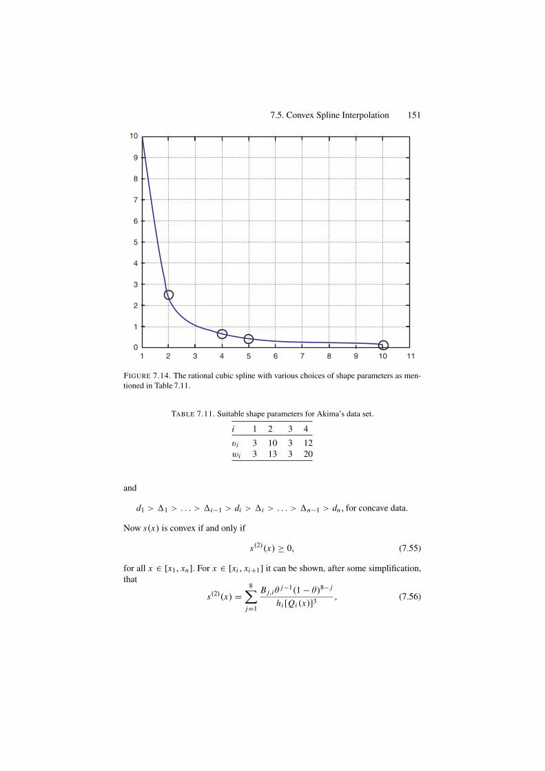
7.5. Convex Spline Interpolation 151
10
9
6
7
8
5
4
3
2
1
01 2 3 4 5 6 7 8 9 10 11
FIGURE 7.14. The rational cubic spline with various choices of shape parameters as men-tioned in Table 7.11.
TABLE 7.11. Suitable shape parameters for Akima’s data set.
i 1 2 3 4
vi 3 10 3 12wi 3 13 3 20
and
d1 > �1 > . . . > �i−1 > di > �i > . . . > �n−1 > dn, for concave data.
Now s(x) is convex if and only if
s(2)(x) ≥ 0, (7.55)
for all x ∈ [x1, xn]. For x ∈ [xi , xi+1] it can be shown, after some simplification,that
s(2)(x) =8∑
j=1
B j,iθj−1(1 − θ)8− j
hi [Qi (x)]3 , (7.56)
152 7. Visualization of Shaped Data by a Rational Cubic Spline
where
B1,i = A2,i − A1,i (2vi − 1) ,B2,i = 2A3,i − A2,i (vi − 2) − A1,i (vi + 4wi ) ,
B3,i = 3A4,i + 3A3,i − 3wi A2,i − 3A1,i (wi + 2) ,B4,i = 4A5,i + 4A4,i (vi + 1) + A3,i (vi − 2wi ) − A2,i (2wi + 5) − 5A1,i ,B5,i = 5A6,i + A5,i (2vi + 5) + A4,i (2vi − wi ) − A3,i (wi − 4) − 4A2,i ,
B6,i = 3A6,i (vi + 2) + 3vi A5,i − 3A4,i − 3A3,i ,B7,i = A6,i (4vi + wi ) + A5,i (wi − 2) − 2A4,i ,
B8,i = A6,i (2wi − 1) − A5,i ,
⎫⎪⎪⎪⎪⎪⎪⎪⎪⎪⎪⎬
⎪⎪⎪⎪⎪⎪⎪⎪⎪⎪⎭
(7.57)
Since the denominator in (7.56), for the selection of vi , wi > 0, is positive, thenthe sufficient conditions for convexity on [xi , xi+1] are:
vi , wi > 0, B j,i ≥ 0, j = 1, 2, . . . , 8, (7.58)
where the necessary conditions
�i − di ≥ 0and di+1 − �i ≥ 0 (7.59)
are assumed. After some simplifications, one can rewrite the first and the last equa-tions, from (7.57), as follows:
B1,i = 2 {(wi − vi ) �i + vi (�i − di ) − (di+1 − di )} ,B8,i = 2 {(wi − vi ) �i + wi (di+1 − �i ) − (di+1 − di )} .
}. (7.60)
If �i − di > 0 and di+1 − �i > 0 (strict inequalities), then the following aresufficient conditions for (7.60):
vi = wi ,vi (�i − di ) − (di+1 − di ) ≥ 0,
wi (di+1 − �i ) − (di+1 − di ) ≥ 0.
⎫⎬
⎭. (7.61)
These are equivalent to the followings constraints:
vi = wi = li + max(
di+1 − di
�i − di,
di+1 − di
di+1 − �i
), (7.62)
where li are non-negative quantities satisfying
li ≥ 0. (7.63)
After some manipulations, it is trivial to show that the sufficient conditions (7.58),for (7.56), are also sufficient for (7.54). Since
di+1 − �i
�i − di+ �i − di
di+1 − �i≥ max
(di+1 − di
�i − di,
di+1 − di
di+1 − �i
). (7.64)
7.5. Convex Spline Interpolation 153
Therefore, the sufficient conditions (7.62) for convexity take the following form:
vi = wi = li + di+1 − �i
�i − di+ �i − di
di+1 − �i, li ≥ 0. (7.65)
However, the following choice of parameters
vi = wi = li + max(
di+1 − di
�i − di,
di+1 − di
di+1 − �i
), li = 0, (7.66)
will be considered for practical implementation of default curve design. Thischoice satisfies (7.62) and it also provides acceptable results.
Remark 7.4. The default value of the parameters li , being taken as zero, leads tothe default constraints:
vi = wi = max(
di+1 − di
�i − di,
di+1 − di
di+1 − �i
), (7.67)
provides visually pleasing results and produces automated curve interpolation.Further modification is achieved by taking other positive values in variousintervals.
Remark 7.5. It should be noted that if �i − di = 0 or di+1 − �i = 0, then it isnecessary to set di = di+1 = �i . The interpolant then will be linear in that region,i.e.,
s(x) = (1 − θ) fi + θ fi+1. (7.68)
It should also be noted that if �i = 0, then it is necessary to set di = di+1 = 0,and thus
s(x) = fi = fi+1 (7.69)
is a constant on [xi , xi+1]. Hence the interpolant (7.6) is convex together with theconditions (7.65). For the case, where the data is convex but not strictly convex,it would be necessary to divide the data into strictly convex parts. If we set di =di+1 = 0 whenever �i = 0, then the resulting interpolant will be C0 at breakpoints.
The above discussion can be summarized as follows:
Theorem 7.4. Given the conditions (7.54) on the derivative parameters and thedata, the constraints (7.65) are the sufficient conditions for the interpolant (7.6) tobe convex.
7.5.1 DemonstrationWe will assume the derivative approximations as mentioned in Subsection 7.2.2.2.The scheme has been implemented on the data set of Table 7.10. Figure 7.13 is thedefault rational cubic spline curve for the choice of parameters in (7.17), whereasFigure 7.15 is its corresponding shape-preserving spline curve for the automaticchoice of parameters in (7.67).
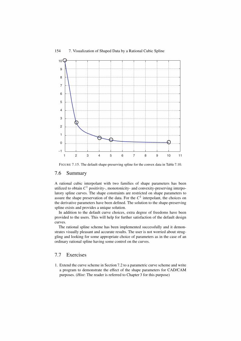
154 7. Visualization of Shaped Data by a Rational Cubic Spline
10
9
8
6
4
5
3
2
1
0
−11 2 3 4 5 6 7 8 9 10 11
7
FIGURE 7.15. The default shape-preserving spline for the convex data in Table 7.10.
7.6 Summary
A rational cubic interpolant with two families of shape parameters has beenutilized to obtain C1 positivity-, monotonicity- and convexity-preserving interpo-latory spline curves. The shape constraints are restricted on shape parameters toassure the shape preservation of the data. For the C1 interpolant, the choices onthe derivative parameters have been defined. The solution to the shape-preservingspline exists and provides a unique solution.
In addition to the default curve choices, extra degree of freedoms have beenprovided to the users. This will help for further satisfaction of the default designcurves.
The rational spline scheme has been implemented successfully and it demon-strates visually pleasant and accurate results. The user is not worried about strug-gling and looking for some appropriate choice of parameters as in the case of anordinary rational spline having some control on the curves.
7.7 Exercises
1. Extend the curve scheme in Section 7.2 to a parametric curve scheme and writea program to demonstrate the effect of the shape parameters for CAD/CAMpurposes. (Hint: The reader is referred to Chapter 3 for this purpose)
References 155
2. Extend the curve scheme in Section 7.3 to a parametric curve scheme such thatit preserves the positive data.
3. Extend the curve scheme in Section 7.4 to a parametric curve scheme such thatit preserves the monotonic data.
4. Extend the curve scheme in Section 7.5 to a parametric curve scheme such thatit preserves the convex data.
5. Write program to visualize the results of the scheme in Exercises 2–4.6. Extend the curve scheme in Section 7.2 to a C2 curve scheme.7. Extend the curve scheme in Section 7.3 to a C2 curve scheme.8. Extend the curve scheme in Section 7.4 to a C2 curve scheme.9. Extend the curve scheme in Section 7.5 to a C2 curve scheme.
References1. McAllister, D.F., and Roulier, J.A. (1981), An algorithm for computing a shape-
preserving osculatory quadratic spline, ACM Trans Math Software 7, 331–347.2. Passow, E., and Roulier, J.A. (1977), Monotone and convex spline interpolation. SIAM
J Num Anal 14, 904–909.3. Fritsch, F.N., and Carlson, R.E. (1980), Monotone piecewise cubic interpolation, SIAM
J Num Anal 17, 238–246.4. Gregory, J.A. (1986), Shape-preserving spline interpolation, Comput Aided Design,
18(1), 53–57.5. Fritsch, F.N., and Butland, J. (1984), A method for constructing local monotone piece-
wise cubic interpolants, SIAM J Sci Stat Comput 5, 303–304.6. Schumaker, L.L. (1983), On shape-preserving quadratic spline interpolation, SIAM J
Num Anal 20, 854–864.7. Brodlie, K.W., and Butt, S. (1991), Preserving convexity using piecewise cubic inter-
polation, Comput Graphics, 15, 15–23.8. Butt, S., and Brodlie, K.W. (1993), Preserving positivity using piecewise cubic inter-
polation, Comput Graphics, 17(1), 55–64.9. Sarfraz, M. (1992), Convexity-preserving piecewise rational interpolation for planar
curves, Bull Korean Math Soc 29(2), 193–200.10. Sarfraz, M. (1997), Preserving monotone shape of the data using piecewise rational
cubic functions, Comput Graphics, 21(1), 5–14.11. Brodlie, K.W. (1985), Methods for drawing curves. In: Fundamenal Algorithm for
Computer Graphics, ed. R.A. Earnshaw, Springer-Verlag, Berlin, pp. 303–323.12. DeVore, A., and Yan, Z. (1986), Error analysis for piecewise quadratic curve-fitting
algorithms, Comp Aided Geom Design 3, 205–215.13. Greiner, K. (1991), A survey on univariate data interpolation and approximation by
splines of given shape, Math Comp Mod 15, 97–106.14. Constantini, P. (1997), Boundary-valued shape preserving interpolating splines, ACM
Trans Math Software, 23(2), 229–251.15. Lahtinen, A. (1996), Monotone interpolation with application to estimation of taper
curves, Ann Numer Math 3, 151–161.16. Sarfraz, M. (1992), Interpolatory rational cubic spline with biased, point and interval
tension, Comput Graphics 16(4), 427–430.

156 7. Visualization of Shaped Data by a Rational Cubic Spline
17. Moreton H.P., and Sequin, C.H. (1995), Minimum variation curves and surfacesfor computer-aided geometric design, Designing Fair Curves and Surfaces, NickSapidis ed., Proc. of SIAM’94 Conference, pp. 123–159.
18. Sarfraz, M., Butt, S., and Hussain, M.Z. (2001), Visualization of shaped data by arational cubic spline interpolation, Int J Comput Graphics, Elsevier Science, 25(5),833–845.
19. Sarfraz, M. (2000), A rational cubic spline for the visualization of monotonic data,Comput Graphics, 24(4), 509–516.
20. Sarfraz, M., and Hussain, M.Z. (2006), Data visualization using rational spline inter-polation, Int Computational Appl Math, Elsevier Science, 189(1–2), 513–525.
21. Sarfraz, M., Hussain, M.Z., and Chaudhry, F.S. (2005), Shape-preserving cubic splinefor data visualization, Int J Comput Graphics CAD/CAM, International Scientific, 1(6),185–194.
22. Sarfraz, M. (2002), Visualization of positive and convex data by a rational cubic spline,Int J Infor Sci, Elsevier Science,146(1–4), 239–254.
23. Sarfraz, M. (2002), Modelling for the visualization of monotone data, Int J ModellingSimulation, ACTA Press, 22(3), 176–185.
8Visualization of Shaped Data by CubicSpline Interpolation
Abstract. This chapter reiterates the subject of the previous chapter. Instead of a rationalcubic model, a polynomial cubic spline has been presented here for the same objective.A piecewise cubic spline has been introduced to preserve the shape of the data when it isconvex, monotone or positive. The spline representation is interpolatory and applicable tothe scalar valued data. The shape parameters, in the description of the cubic, have beenconstrained in such a way that they control the shape of the curve to avoid any noise. Asfar as visual smoothness is concerned, the curve scheme under discussion is GC1. Thus thecontinuity constraints have been relaxed from C1 to GC1.
8.1 Introduction
This chapter is a continuation of the previous chapter. The difference arisesmainly in two ways: (i) the interpolant used is a piecewise cubic polynomial, and(ii) visual smoothness is of the curve scheme under discussion, which is GC1.Thus, the continuity constraints have been relaxed from C1 to GC1 to obtain ashape-preserving cubic spline.
The early work in this chapter was reported in [17] and further extension ofthe preliminary work was achieved in [18]. The shape-preserving techniques pre-sented here are an economical alternative to their counterparts in the previouschapter as well as in [1–16]. The methods under consideration in this chapterhave the following important and advantageous features that no additional points(knots) need to be supplied. In contrast, the cubic interpolation method of Brodlieand Butt [1, 2] requires the introduction of additional knots when used as shape-preserving methods. Moreover, existing algorithms such as the de Castlejau algo-rithm can be used for rapid computations.
The chapter is organized so that Section 8.2 describes the Hermite-like cubicinterpolation. An introduction to shape-preserving is provided in Section 8.3. Theproblems of convexity, monotonicity and positivity are discussed in Sections 8.4,8.5 and 8.6, respectively. Section 8.7 is devoted to the extension of positivity whena data is above an arbitrary line. Section 8.8 summarizes the chapter.
157
158 8. Visualization of Shaped Data by Cubic Spline Interpolation
8.2 Cubic Interpolant
Let (xi , fi ) , i = 1, 2, . . . , n, be a given set of data points, where x1 < x2 < · · · <xn . Let
hi = xi+1 − xi , �i = fi+1 − fi
hi, i = 1, 2, . . . , n − 1. (8.1)
Consider the following piecewise cubic function:
S (x) ≡ Si (x) = Ui (1 − θ)3 + 3Viθ (1 − θ)2 + 3Wiθ2 (1 − θ) + Ziθ
3, (8.2)
whereθ = x − xi
hi. (8.3)
To make the function (8.2) GC1, one needs to impose the following interpolatoryproperties:
S (xi ) = fi , and S (xi+1) = fi+1, S(1) (xi ) = di
ri, and S(1) (xi+1) = di+1
ri,
(8.4)which provide the following manipulations:
Ui = fi , Zi = fi+1, Vi = fi + hi di
3ri, and Wi = fi+1 − hi di+1
3ri, (8.5)
where S(1)(x) denotes derivative with respect to x and di denotes derivative valuegiven at the knot xi . This leads the piecewise cubic (8.2) to the following piecewiseHermite-like interpolant S ∈ C1 [x1, xn]:
S (x) ≡ Si (x) , (8.6)
where
Si (x) = fi (1 − θ)3 + 3Viθ (1 − θ)2 + 3Wiθ2 (1 − θ) + fi+1θ
3. (8.7)
The parameters ri ’s, and the derivatives di ’s are to be chosen such that the shapeof the data is preserved by the interpolant (8.6). One can note that when ri = 1,the cubic function obviously becomes the standard cubic Hermite polynomial.Variation for the values of ri ’s control (tighten or loosen) the curve in differentpieces of the curve. When ri → 0, it is simple to see that the curve gets tightenedin the corresponding interval. This interval shape control behavior is desired asa constraint so that the interpolant automatically becomes convex to the convexdata, monotone to monotone data and positive to positive data.
It should be noted that the shape control analysis is valid only if the boundedderivative values are assumed. In most applications, the derivative parameters{di } are not given and hence must be determined either from the given data(xi , fi ) , i = 1, 2, . . . , n, or by some other means. In this chapter, they are com-puted exactly in the same way as in Section 8.8.2 of the previous chapter. Thesmoothness of the interpolant (8.6), hence would be GC1.
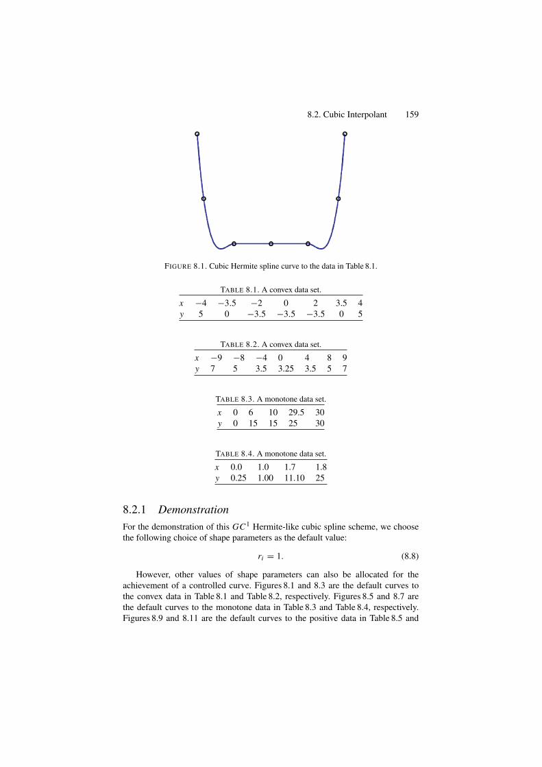
8.2. Cubic Interpolant 159
FIGURE 8.1. Cubic Hermite spline curve to the data in Table 8.1.
TABLE 8.1. A convex data set.
x −4 −3.5 −2 0 2 3.5 4y 5 0 −3.5 −3.5 −3.5 0 5
TABLE 8.2. A convex data set.
x −9 −8 −4 0 4 8 9y 7 5 3.5 3.25 3.5 5 7
TABLE 8.3. A monotone data set.
x 0 6 10 29.5 30y 0 15 15 25 30
TABLE 8.4. A monotone data set.
x 0.0 1.0 1.7 1.8y 0.25 1.00 11.10 25
8.2.1 DemonstrationFor the demonstration of this GC1 Hermite-like cubic spline scheme, we choosethe following choice of shape parameters as the default value:
ri = 1. (8.8)
However, other values of shape parameters can also be allocated for theachievement of a controlled curve. Figures 8.1 and 8.3 are the default curves tothe convex data in Table 8.1 and Table 8.2, respectively. Figures 8.5 and 8.7 arethe default curves to the monotone data in Table 8.3 and Table 8.4, respectively.Figures 8.9 and 8.11 are the default curves to the positive data in Table 8.5 and
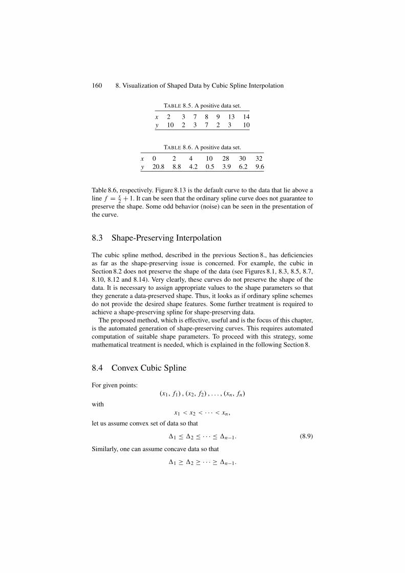
160 8. Visualization of Shaped Data by Cubic Spline Interpolation
TABLE 8.5. A positive data set.
x 2 3 7 8 9 13 14y 10 2 3 7 2 3 10
TABLE 8.6. A positive data set.
x 0 2 4 10 28 30 32y 20.8 8.8 4.2 0.5 3.9 6.2 9.6
Table 8.6, respectively. Figure 8.13 is the default curve to the data that lie above aline f = x
2 + 1. It can be seen that the ordinary spline curve does not guarantee topreserve the shape. Some odd behavior (noise) can be seen in the presentation ofthe curve.
8.3 Shape-Preserving Interpolation
The cubic spline method, described in the previous Section 8., has deficienciesas far as the shape-preserving issue is concerned. For example, the cubic inSection 8.2 does not preserve the shape of the data (see Figures 8.1, 8.3, 8.5, 8.7,8.10, 8.12 and 8.14). Very clearly, these curves do not preserve the shape of thedata. It is necessary to assign appropriate values to the shape parameters so thatthey generate a data-preserved shape. Thus, it looks as if ordinary spline schemesdo not provide the desired shape features. Some further treatment is required toachieve a shape-preserving spline for shape-preserving data.
The proposed method, which is effective, useful and is the focus of this chapter,is the automated generation of shape-preserving curves. This requires automatedcomputation of suitable shape parameters. To proceed with this strategy, somemathematical treatment is needed, which is explained in the following Section 8.
8.4 Convex Cubic Spline
For given points:(x1, f1) , (x2, f2) , . . . , (xn, fn)
withx1 < x2 < · · · < xn,
let us assume convex set of data so that
�1 ≤ �2 ≤ · · · ≤ �n−1. (8.9)
Similarly, one can assume concave data so that
�1 ≥ �2 ≥ · · · ≥ �n−1.
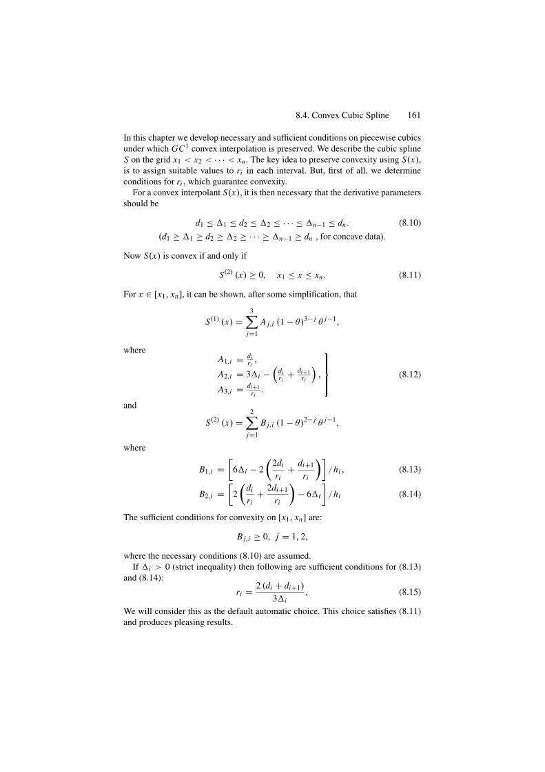
8.4. Convex Cubic Spline 161
In this chapter we develop necessary and sufficient conditions on piecewise cubicsunder which GC1 convex interpolation is preserved. We describe the cubic splineS on the grid x1 < x2 < · · · < xn . The key idea to preserve convexity using S(x),is to assign suitable values to ri in each interval. But, first of all, we determineconditions for ri , which guarantee convexity.
For a convex interpolant S(x), it is then necessary that the derivative parametersshould be
d1 ≤ �1 ≤ d2 ≤ �2 ≤ · · · ≤ �n−1 ≤ dn . (8.10)(d1 ≥ �1 ≥ d2 ≥ �2 ≥ · · · ≥ �n−1 ≥ dn , for concave data).
Now S(x) is convex if and only if
S(2) (x) ≥ 0, x1 ≤ x ≤ xn . (8.11)
For x ∈ [x1, xn], it can be shown, after some simplification, that
S(1) (x) =3∑
j=1
A j,i (1 − θ)3− j θ j−1,
whereA1,i = di
ri,
A2,i = 3�i −(
diri
+ di+1ri
),
A3,i = di+1ri
.
⎫⎪⎪⎬
⎪⎪⎭(8.12)
and
S(2) (x) =2∑
j=1
B j,i (1 − θ)2− j θ j−1,
where
B1,i =[
6�i − 2(
2di
ri+ di+1
ri
)]/hi , (8.13)
B2,i =[
2(
di
ri+ 2di+1
ri
)− 6�i
]/hi (8.14)
The sufficient conditions for convexity on [x1, xn] are:
B j,i ≥ 0, j = 1, 2,
where the necessary conditions (8.10) are assumed.If �i > 0 (strict inequality) then following are sufficient conditions for (8.13)
and (8.14):
ri = 2 (di + di+1)
3�i, (8.15)
We will consider this as the default automatic choice. This choice satisfies (8.11)and produces pleasing results.
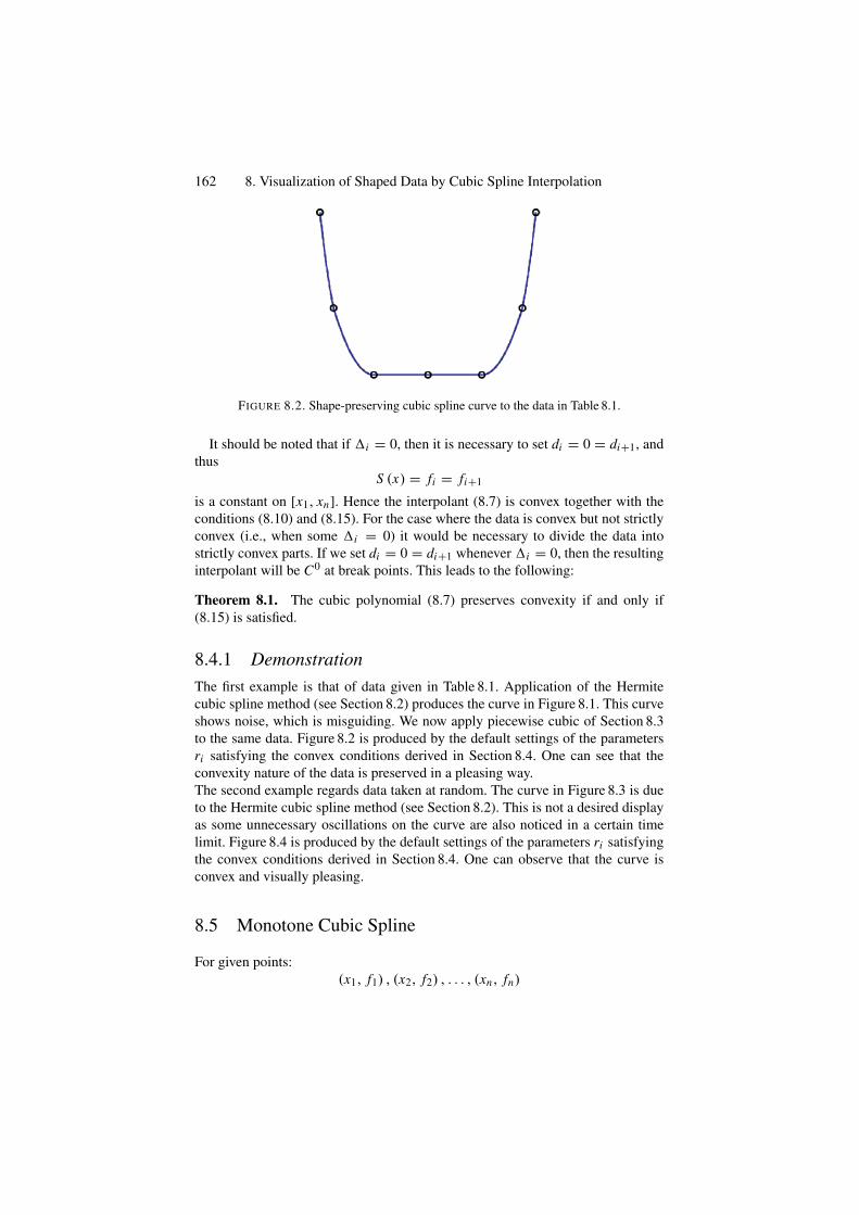
162 8. Visualization of Shaped Data by Cubic Spline Interpolation
FIGURE 8.2. Shape-preserving cubic spline curve to the data in Table 8.1.
It should be noted that if �i = 0, then it is necessary to set di = 0 = di+1, andthus
S (x) = fi = fi+1
is a constant on [x1, xn]. Hence the interpolant (8.7) is convex together with theconditions (8.10) and (8.15). For the case where the data is convex but not strictlyconvex (i.e., when some �i = 0) it would be necessary to divide the data intostrictly convex parts. If we set di = 0 = di+1 whenever �i = 0, then the resultinginterpolant will be C0 at break points. This leads to the following:
Theorem 8.1. The cubic polynomial (8.7) preserves convexity if and only if(8.15) is satisfied.
8.4.1 DemonstrationThe first example is that of data given in Table 8.1. Application of the Hermitecubic spline method (see Section 8.2) produces the curve in Figure 8.1. This curveshows noise, which is misguiding. We now apply piecewise cubic of Section 8.3to the same data. Figure 8.2 is produced by the default settings of the parametersri satisfying the convex conditions derived in Section 8.4. One can see that theconvexity nature of the data is preserved in a pleasing way.The second example regards data taken at random. The curve in Figure 8.3 is dueto the Hermite cubic spline method (see Section 8.2). This is not a desired displayas some unnecessary oscillations on the curve are also noticed in a certain timelimit. Figure 8.4 is produced by the default settings of the parameters ri satisfyingthe convex conditions derived in Section 8.4. One can observe that the curve isconvex and visually pleasing.
8.5 Monotone Cubic Spline
For given points:(x1, f1) , (x2, f2) , . . . , (xn, fn)
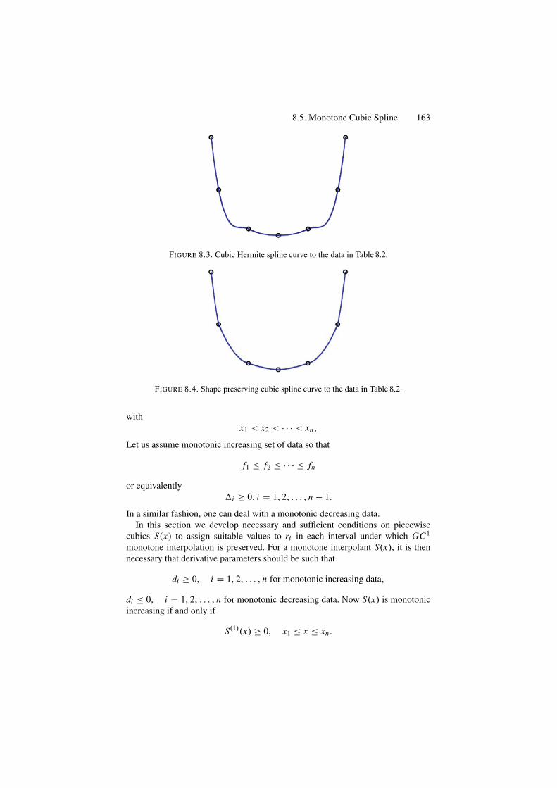
8.5. Monotone Cubic Spline 163
FIGURE 8.3. Cubic Hermite spline curve to the data in Table 8.2.
FIGURE 8.4. Shape preserving cubic spline curve to the data in Table 8.2.
withx1 < x2 < · · · < xn,
Let us assume monotonic increasing set of data so that
f1 ≤ f2 ≤ · · · ≤ fn
or equivalently�i ≥ 0, i = 1, 2, . . . , n − 1.
In a similar fashion, one can deal with a monotonic decreasing data.In this section we develop necessary and sufficient conditions on piecewise
cubics S(x) to assign suitable values to ri in each interval under which GC1
monotone interpolation is preserved. For a monotone interpolant S(x), it is thennecessary that derivative parameters should be such that
di ≥ 0, i = 1, 2, . . . , n for monotonic increasing data,
di ≤ 0, i = 1, 2, . . . , n for monotonic decreasing data. Now S(x) is monotonicincreasing if and only if
S(1)(x) ≥ 0, x1 ≤ x ≤ xn .
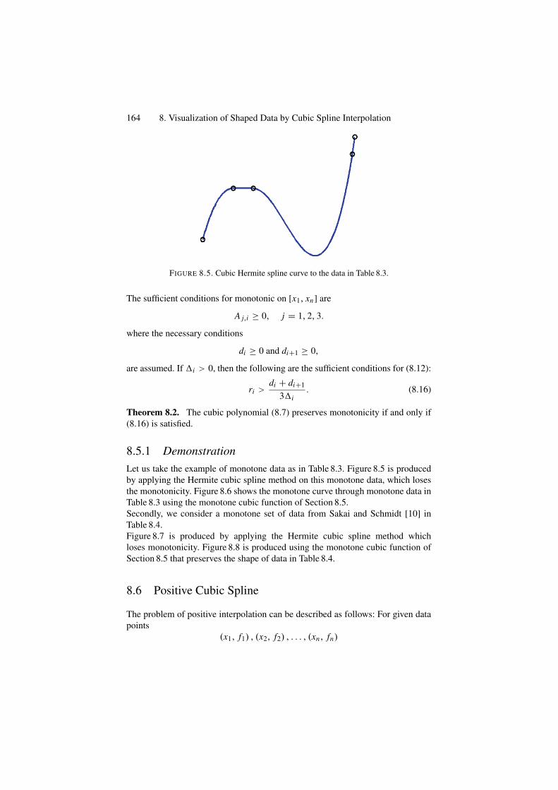
164 8. Visualization of Shaped Data by Cubic Spline Interpolation
FIGURE 8.5. Cubic Hermite spline curve to the data in Table 8.3.
The sufficient conditions for monotonic on [x1, xn] are
A j,i ≥ 0, j = 1, 2, 3.
where the necessary conditions
di ≥ 0 and di+1 ≥ 0,
are assumed. If �i > 0, then the following are the sufficient conditions for (8.12):
ri >di + di+1
3�i. (8.16)
Theorem 8.2. The cubic polynomial (8.7) preserves monotonicity if and only if(8.16) is satisfied.
8.5.1 DemonstrationLet us take the example of monotone data as in Table 8.3. Figure 8.5 is producedby applying the Hermite cubic spline method on this monotone data, which losesthe monotonicity. Figure 8.6 shows the monotone curve through monotone data inTable 8.3 using the monotone cubic function of Section 8.5.Secondly, we consider a monotone set of data from Sakai and Schmidt [10] inTable 8.4.Figure 8.7 is produced by applying the Hermite cubic spline method whichloses monotonicity. Figure 8.8 is produced using the monotone cubic function ofSection 8.5 that preserves the shape of data in Table 8.4.
8.6 Positive Cubic Spline
The problem of positive interpolation can be described as follows: For given datapoints
(x1, f1) , (x2, f2) , . . . , (xn, fn)
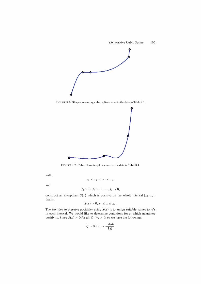
8.6. Positive Cubic Spline 165
FIGURE 8.6. Shape-preserving cubic spline curve to the data in Table 8.3.
FIGURE 8.7. Cubic Hermite spline curve to the data in Table 8.4.
withx1 < x2 < · · · < xn,
andf1 > 0, f2 > 0, . . . , fn > 0,
construct an interpolant S(x) which is positive on the whole interval [x1, xn],that is,
S(x) > 0, x1 ≤ x ≤ xn .
The key idea to preserve positivity using S(x) is to assign suitable values to ri ’sin each interval. We would like to determine conditions for ri which guaranteepositivity. Since S(x) > 0 for all Vi , Wi > 0, so we have the following:
Vi > 0 if ri >−hi di
3 fi,
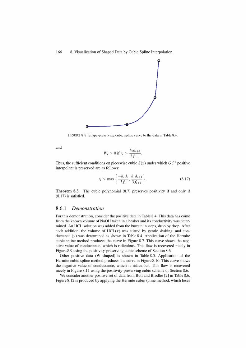
166 8. Visualization of Shaped Data by Cubic Spline Interpolation
FIGURE 8.8. Shape-preserving cubic spline curve to the data in Table 8.4.
andWi > 0 if ri >
hi di+1
3 fi+1.
Thus, the sufficient conditions on piecewise cubic S(x) under which GC1 positiveinterpolant is preserved are as follows:
ri > max{−hi di
3 fi,
hi di+1
3 fi+1
}. (8.17)
Theorem 8.3. The cubic polynomial (8.7) preserves positivity if and only if(8.17) is satisfied.
8.6.1 DemonstrationFor this demonstration, consider the positive data in Table 8.4. This data has comefrom the known volume of NaOH taken in a beaker and its conductivity was deter-mined. An HCL solution was added from the burette in steps, drop by drop. Aftereach addition, the volume of HCL(x) was stirred by gentle shaking, and con-ductance (y) was determined as shown in Table 8.4. Application of the Hermitecubic spline method produces the curve in Figure 8.7. This curve shows the neg-ative value of conductance, which is ridiculous. This flaw is recovered nicely inFigure 8.9 using the positivity-preserving cubic scheme of Section 8.6.
Other positive data (W shaped) is shown in Table 8.5. Application of theHermite cubic spline method produces the curve in Figure 8.10. This curve showsthe negative value of conductance, which is ridiculous. This flaw is recoverednicely in Figure 8.11 using the positivity-preserving cubic scheme of Section 8.6.
We consider another positive set of data from Butt and Brodlie [2] in Table 8.6.Figure 8.12 is produced by applying the Hermite cubic spline method, which loses
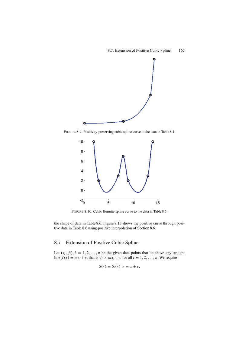
8.7. Extension of Positive Cubic Spline 167
FIGURE 8.9. Positivity-preserving cubic spline curve to the data in Table 8.4.
FIGURE 8.10. Cubic Hermite spline curve to the data in Table 8.5.
the shape of data in Table 8.6. Figure 8.13 shows the positive curve through posi-tive data in Table 8.6 using positive interpolation of Section 8.6.
8.7 Extension of Positive Cubic Spline
Let (xi , fi ), i = 1, 2, . . . , n be the given data points that lie above any straightline f (x) = mx + c, that is fi > mxi + c for all i = 1, 2, . . . , n. We require
S(x) ≡ Si (x) > mxi + c.
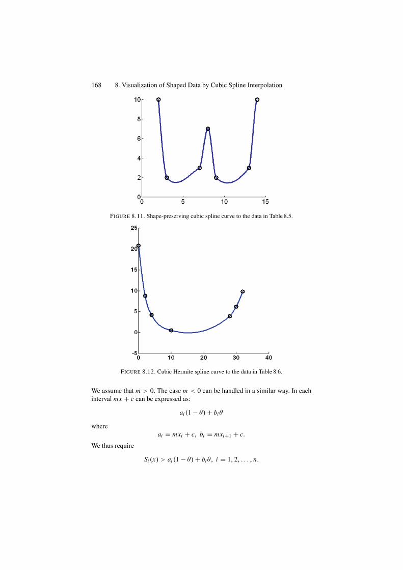
168 8. Visualization of Shaped Data by Cubic Spline Interpolation
FIGURE 8.11. Shape-preserving cubic spline curve to the data in Table 8.5.
FIGURE 8.12. Cubic Hermite spline curve to the data in Table 8.6.
We assume that m > 0. The case m < 0 can be handled in a similar way. In eachinterval mx + c can be expressed as:
ai (1 − θ) + biθ
whereai = mxi + c, bi = mxi+1 + c.
We thus require
Si (x) > ai (1 − θ) + biθ, i = 1, 2, . . . , n.
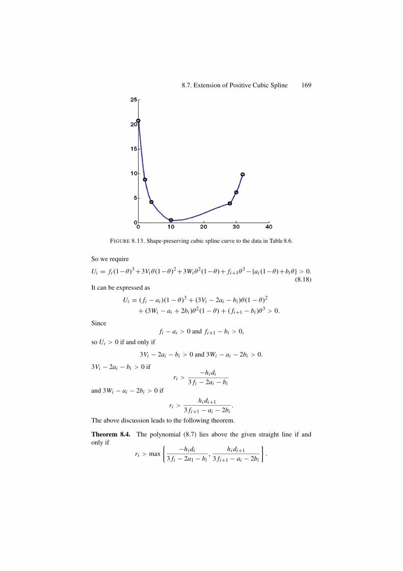
8.7. Extension of Positive Cubic Spline 169
FIGURE 8.13. Shape-preserving cubic spline curve to the data in Table 8.6.
So we require
Ui = fi (1−θ)3 +3Viθ(1−θ)2 +3Wiθ2(1−θ)+ fi+1θ
3 −{ai (1−θ)+biθ} > 0.(8.18)
It can be expressed as
Ui = ( fi − ai )(1 − θ)3 + (3Vi − 2ai − bi )θ(1 − θ)2
+ (3Wi − ai + 2bi )θ2(1 − θ) + ( fi+1 − bi )θ
3 > 0.
Sincefi − ai > 0 and fi+1 − bi > 0,
so Ui > 0 if and only if
3Vi − 2ai − bi > 0 and 3Wi − ai − 2bi > 0.
3Vi − 2ai − bi > 0 if
ri >−hi di
3 fi − 2ai − biand 3Wi − ai − 2bi > 0 if
ri >hi di+1
3 fi+1 − ai − 2bi.
The above discussion leads to the following theorem.
Theorem 8.4. The polynomial (8.7) lies above the given straight line if andonly if
ri > max{ −hi di
3 fi − 2a1 − bi,
hi di+1
3 fi+1 − ai − 2bi
}.
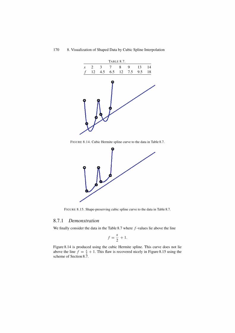
170 8. Visualization of Shaped Data by Cubic Spline Interpolation
TABLE 8.7.
x 2 3 7 8 9 13 14f 12 4.5 6.5 12 7.5 9.5 18
FIGURE 8.14. Cubic Hermite spline curve to the data in Table 8.7.
FIGURE 8.15. Shape-preserving cubic spline curve to the data in Table 8.7.
8.7.1 DemonstrationWe finally consider the data in the Table 8.7 where f -values lie above the line
f = x2
+ 1.
Figure 8.14 is produced using the cubic Hermite spline. This curve does not lieabove the line f = x
2 + 1. This flaw is recovered nicely in Figure 8.15 using thescheme of Section 8.7.
References 171
Remark 8.1. These methods can be used in both cases when either di ’s are par-ticularly specified or estimated by some method. We propose the arithmetic meanapproximation method [3] for the practical implementation in this chapter.
8.8 Summary
A piecewise cubic interpolant, in a generalized form, has been utilized to obtaina GC1 convexity-, monotonicity- and positivity-preserving curve methods. Data-dependent shape constraints are derived on shape parameters to assure the shapepreservation of the data. Choice of the derivative parameters is considered to bethe approximation through arithmetic choice.
The proposed curve schemes are visually smooth enough and present reason-ably acceptable demonstrations of the shape of the data, but a higher degree ofsmoothness, while stitching the pieces of curves, may enhance the visual display.
8.9 Exercises
1. Extend the curve scheme in Section 8.2 to a parametric curve scheme and writea program to demonstrate the effect of the shape parameters for CAD/CAMpurposes.
2. Extend the curve scheme in Section 8.4 to a parametric curve scheme such thatit preserves the convex data.
3. Extend the curve scheme in Section 8.5 to a parametric curve scheme such thatit preserves the monotonic data.
4. Extend the curve scheme in Section 8.6 to a parametric curve scheme such thatit preserves the positive data.
5. Write a program to visualize the results of the scheme in Exercises 4–6.6. Extend the curve scheme in Section 8.2 to a C1 curve scheme.7. Extend the curve scheme in Section 8.4 to a C1 curve scheme.8. Extend the curve scheme in Section 8.5 to a C1 curve scheme.9. Extend the curve scheme in Section 8.6 to a C1 curve scheme.
References1. Brodlie, K.W., and Butt, S. (1991), Preserving convexity using piecewise cubic inter-
polation, Comput Graphics 15(1), 15–23.2. Butt, S., and Brodlie, K.W. (1993), Preserving positivity using piecewise cubic inter-
polation, Comput Graphics 17(1), 55–64.3. Delbourgo, R., and Gregory, J.A. (1985), Shape-preserving piecewise rational interpo-
lation, SIAM J Stat Comput 6, 967–976.4. Fritsch, F.N., and Butland, J. (1984), A method for constructing local monotone piece-
wise cubic interpolants, SIAM J Sci Stat Comput 5, 300–304.5. Fritsch, F.N., and Carlson, R.E. (1980), Monotone piecewise cubic interpolation, SIAM
J Numer Anal 17(2), 238–246.

172 8. Visualization of Shaped Data by Cubic Spline Interpolation
6. Gregory, J.A., and Sarfraz, M. (1990), A rational spline with tension, Comput AidedGeom Des 7, 1–13.
7. Gregory, J.R., and Delbourgo, R. (1983), Piecewise rational quadratic interpolation tomonotonic data, SIAM J Numer Anal 3, 141–152.
8. McAllister, D.F., Passow, E., and Roulier, J.A. (1977), Algorithms for computingshape-preserving spline interpolations to data, Math Comp 31, 717–725.
9. McAllister, D.F., and Roulier, J.A. (1981), An algorithm for computing a shape-preserving osculatory quadratic spline, ACM Trans Math Software 7, 331–347.
10. Sakai, M., and Schmidt, J.W. (1988), Positive interpolation with rational splines,Computing, 140–147.
11. Sarfraz, M. (1992), Convexity-preserving piecewise rational interpolation for planarcurves, Bull Korean Math Soc 29(2), 193–200.
12. Sarfraz, M., Al-Mulhem, M., and Ashraf, F. (1997), Preserving monotonic shape of thedata using piecewise rational cubic functions, Comput Graphics 21(1), 5–14.
13. Sarfraz, M. (2003), A rational cubic spline for the visualization of monotonic data: analternate approach, Int J Comput Graphics, Elsevier Science, 27(1), 107–121.
14. Sarfraz, M. (2002), Visualization of positive and convex data by a rational cubic spline,Int J Information Sci, Elsevier Science Inc., 146(1–4), 239–254.
15. Sarfraz, M., Butt, S., and Hussain, M.Z. (2001), Visualization of shaped data by arational cubic spline interpolation, Int J Comput Graphics, Elsevier Science, 25(5),833–845.
16. Sarfraz, M. (2000), A rational cubic spline for the visualization of monotonic data, IntJ Comput Graphics, Elsevier Science, 24(4), 509–516.
17. Sarfraz, M., Hussain, M.Z., Chaudhry, F.S. (2005), Shape-preserving data visualizationwith cubic splines, Proceedings of the International Joint Conference on InformationSciences-JCIS’2005-USA, Etienne E. Kerre, Donald Hung, Dan Ventura, Manuel GranaRomay, Heng-Da Cheng, Hong Va Leong, Shu-Heng Chen, David K.Y. Chiu, SteveBlair, Paul P. Wang, Chris Tseng, Chang-Tien Lu, Jie Lu, M. Sarfraz (Eds.), pp. 1661–1664.
18. Sarfraz, M., Hussain, M.Z., and Chaudhry, F.S. (2005), Shape-preserving cubic splinefor data visualization, Int J Comput Graphics CAD/CAM, International Scientific 1(6),185-194.
9Approximation with B-Splines Curves
Abstract. B-spline curves have been used to approximate the functional data. Two curveapproximation techniques are presented here. One scheme is based on a deterministicapproach using quadratic B-splines. The other scheme uses a genetic algorithm in its for-mulation where the B-spline can have any order. Both schemes automatically compute datapoints to minimize errors.
9.1 Introduction
Curve approximation [6,8–14] is all about finding accurate locations of data pointsfrom the given curve. It is an important area of computer graphics and can beutilized in computer vision and imaging applications too. B-splines curves [4] arepopular models for curve design and can be defined by their degrees and controlpoints. They have been used here to present curve approximating techniques. Bothof the schemes presented in this chapter automatically compute data points tominimize errors. These techniques can be useful for efficient storage of geometricshapes in any applications of graphics, vision and imaging. The first techniquepresented is based on a deterministic approach; it uses a quadratic B-spline curvefor approximating functions or functional data. The second scheme is based ona nondeterministic approach, namely, a genetic algorithm. It has the freedom toutilize any degree B-spline formulation.
In the first technique [12] presented here, quadratic B-spline data points arecomputed by exploiting the properties of its knots. This technique consists of threesteps of approximation. Step 1 involves computation/plotting of opening angles.In Step 2, knots are inserted at appropriate locations, which bring approxima-tion error within specified threshold limits. Step 3 is a further optimization ofapproximation results by changing knot positions. A general quadratic B-splinecurve through these data points (control points and knots) would be an approx-imating curve. Demonstrated results will show that very precise approximationcan be achieved with quite lesser data points. This curve approximation techniqueis simple, efficient and robust for any parametric curve(s). It does not require anextensive search for data points. Data points once computed are not discarded.
173
174 9. Approximation with B-Splines Curves
The second technique is also based on B-spline formulation [13,14]; it has morefreedom and can use any degree B-spline formulation for curve representation.A genetic approach has been adopted to locate appropriate B-spline knots so thatthe approximation error is minimized.
The rest of the chapter is organized as follows. Section 9.2 gives a generaldescription of quadratic B-splines. Section 9.3 highlights properties of knotstogether with the approximating technique (in three steps). Section 9.4 describesthe technique based on a genetic algorithm (GA). Both schemes have been illus-trated with examples. Section 9.5 summarizes the chapter.
9.2 B-Splines
The general expression for calculation of any coordinate position along a B-splinecurve in a blending function formulation [5] can be given as:
P (u) =n∑
k=0
pk Bk,d (u) ,umin ≤ u ≤ umax, 2 ≤ d ≤ n + 1 (9.1)
In Equation (9.1) above, pk is an input set of n + 1 control points. The B-splineblending function Bk,d are polynomials of degree d − 1. Blending functions forB-spline curves can be defined by the Cox-deBoor recursion formulas [3]:
Bk,d (u) = u − uk
uk+d−1 − ukBk,d−1 (u) + uk+d − u
uk+d − uk+1Bk+1,d−1 (u)
Bk,1 (u) ={
1, if uk ≤ u < uk+10, otherwise
⎫⎪⎪⎬
⎪⎪⎭(9.2)
Each blending function is defined over d subintervals of the total range of u. Wecan choose any values for the subinterval endpoints u j satisfying the relation u j ≤u j+1.
9.3 Deterministic Approach
In this section, we assign d = 3, umin = 0 & umax = 1 for the quadratic B-spline(QBS) curves that would be used for approximation of given curves. The range ofparameter u is divided into n + d + 1 knot values labeled as {u0, u1, . . ., un+d}and the resulting QBS curve is defined in the range from knot value ud−1 up toun+1. For the uniform QBS, the spacing between knots remains constant as in{0.0, 0.2, 0.4, 0.6, 0.8, 1.0}. Figure 9.1 shows QBS with five control points anduniform knot spacing. For the open uniform QBS, the knot spacing is uniformexcept at the ends where knot values are repeated d times as given below:
{0, 0, 0, 0.25, 0.5, 0.75, 1, 1, 1} for d = 3 and n = 5 (9.3)
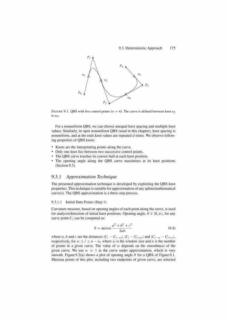
9.3. Deterministic Approach 175
P0
P2
P1
P4
P3
u2
u3
u5
u4
FIGURE 9.1. QBS with five control points (n = 4). The curve is defined between knot u2to u5.
For a nonuniform QBS, we can choose unequal knot spacing and multiple knotvalues. Similarly, in open nonuniform QBS (used in this chapter), knot spacing isnonuniform, and at the ends knot values are repeated d times. We observe follow-ing properties of QBS knots:
• Knots are the interpolating points along the curve.• Only one knot lies between two successive control points.• The QBS curve touches its convex hull at each knot position.• The opening angle along the QBS curve maximizes at its knot positions
(Section 9.3).
9.3.1 Approximation TechniqueThe presented approximation technique is developed by exploiting the QBS knotproperties. This technique is suitable for approximation of any spline/mathematicalcurve(s). The QBS approximation is a three-step process.
9.3.1.1 Initial Data Points (Step 1)
Curvature measure, based on opening angles of each point along the curve, is usedfor analysis/detection of initial knot positions. Opening angle, θ ∈ |0, π |, for anycurve point Ci can be computed as:
θ = arccosa2 + b2 + c2
2ab(9.4)
where a, b and c are the distances |Ci − Ci−w|, |Ci − Ci+w| and |Ci−w − Ci+w|,respectively, for w ≤ i ≤ n − w, where w is the window size and n is the numberof points in a given curve. The value of w depends on the smoothness of thegiven curve. We use w = 1 as the curve under approximation, which is verysmooth. Figure 9.2(a) shows a plot of opening angle θ for a QBS of Figure 9.1.Maxima points of this plot, including two endpoints of given curve, are selected
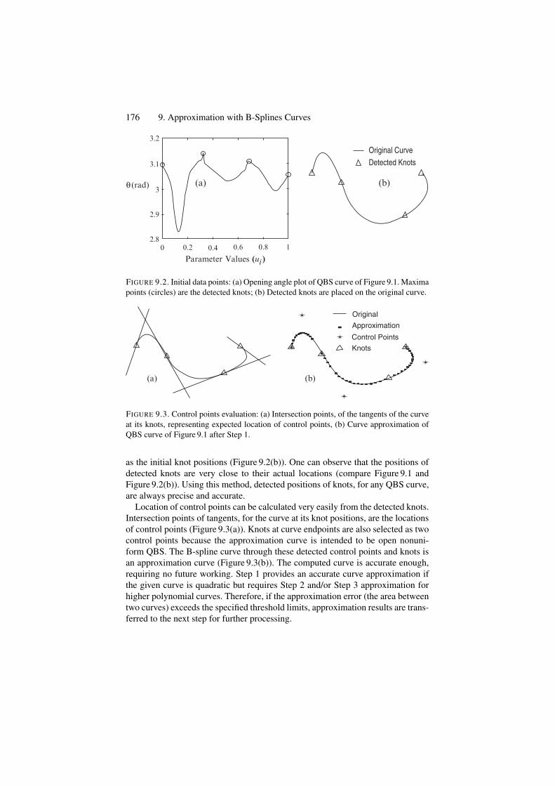
176 9. Approximation with B-Splines Curves
θ (rad)
Parameter Values (ui )
3.2
3.1
3
2.9
2.80 0.2 0.60.4 0.8 1
(b)(a)
Original Curve
Detected Knots
FIGURE 9.2. Initial data points: (a) Opening angle plot of QBS curve of Figure 9.1. Maximapoints (circles) are the detected knots; (b) Detected knots are placed on the original curve.
(a) (b)
Original
Approximation
Control Points
Knots
FIGURE 9.3. Control points evaluation: (a) Intersection points, of the tangents of the curveat its knots, representing expected location of control points, (b) Curve approximation ofQBS curve of Figure 9.1 after Step 1.
as the initial knot positions (Figure 9.2(b)). One can observe that the positions ofdetected knots are very close to their actual locations (compare Figure 9.1 andFigure 9.2(b)). Using this method, detected positions of knots, for any QBS curve,are always precise and accurate.
Location of control points can be calculated very easily from the detected knots.Intersection points of tangents, for the curve at its knot positions, are the locationsof control points (Figure 9.3(a)). Knots at curve endpoints are also selected as twocontrol points because the approximation curve is intended to be open nonuni-form QBS. The B-spline curve through these detected control points and knots isan approximation curve (Figure 9.3(b)). The computed curve is accurate enough,requiring no future working. Step 1 provides an accurate curve approximation ifthe given curve is quadratic but requires Step 2 and/or Step 3 approximation forhigher polynomial curves. Therefore, if the approximation error (the area betweentwo curves) exceeds the specified threshold limits, approximation results are trans-ferred to the next step for further processing.
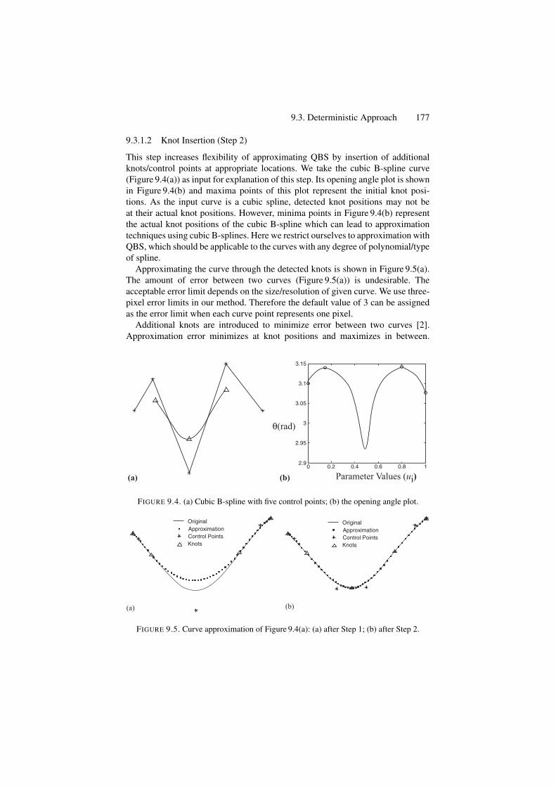
9.3. Deterministic Approach 177
9.3.1.2 Knot Insertion (Step 2)
This step increases flexibility of approximating QBS by insertion of additionalknots/control points at appropriate locations. We take the cubic B-spline curve(Figure 9.4(a)) as input for explanation of this step. Its opening angle plot is shownin Figure 9.4(b) and maxima points of this plot represent the initial knot posi-tions. As the input curve is a cubic spline, detected knot positions may not beat their actual knot positions. However, minima points in Figure 9.4(b) representthe actual knot positions of the cubic B-spline which can lead to approximationtechniques using cubic B-splines. Here we restrict ourselves to approximation withQBS, which should be applicable to the curves with any degree of polynomial/typeof spline.
Approximating the curve through the detected knots is shown in Figure 9.5(a).The amount of error between two curves (Figure 9.5(a)) is undesirable. Theacceptable error limit depends on the size/resolution of given curve. We use three-pixel error limits in our method. Therefore the default value of 3 can be assignedas the error limit when each curve point represents one pixel.
Additional knots are introduced to minimize error between two curves [2].Approximation error minimizes at knot positions and maximizes in between.
(a) (b) Parameter Values (ui)
θ(rad)
3.15
3.1
3.05
3
2.95
2.90 0.2 0.4 0.6 0.8 1
FIGURE 9.4. (a) Cubic B-spline with five control points; (b) the opening angle plot.
Original
KnotsControl PointsApproximation
Original
KnotsControl PointsApproximation
(b)(a)
FIGURE 9.5. Curve approximation of Figure 9.4(a): (a) after Step 1; (b) after Step 2.
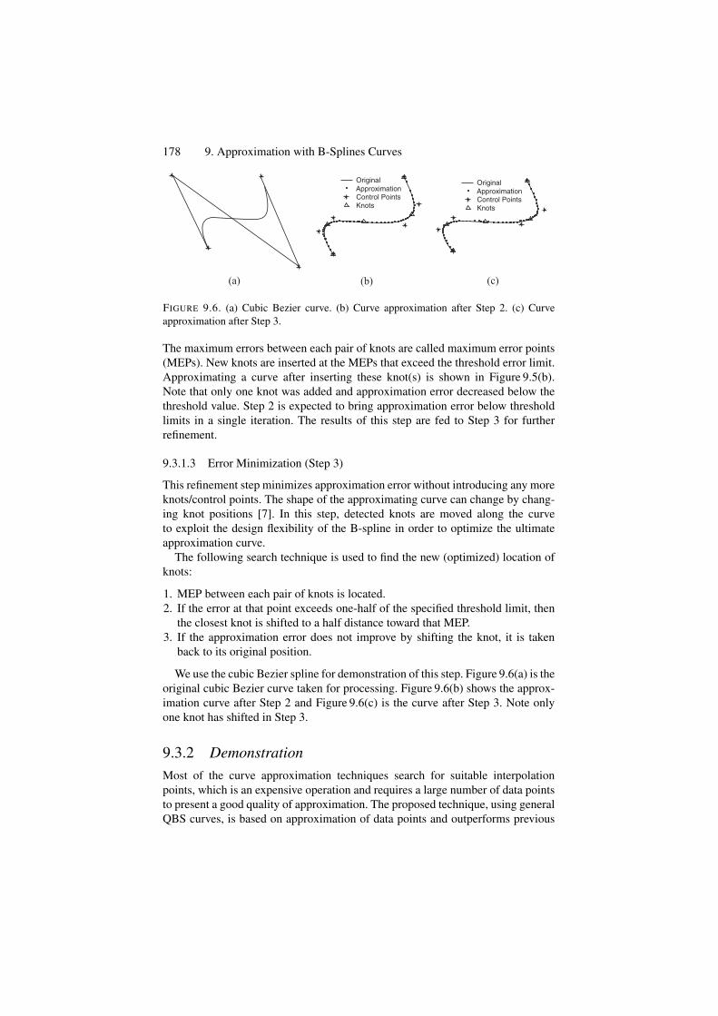
178 9. Approximation with B-Splines Curves
Original
Control PointsKnots
ApproximationOriginal
Control PointsKnots
Approximation
(b)(a) (c)
FIGURE 9.6. (a) Cubic Bezier curve. (b) Curve approximation after Step 2. (c) Curveapproximation after Step 3.
The maximum errors between each pair of knots are called maximum error points(MEPs). New knots are inserted at the MEPs that exceed the threshold error limit.Approximating a curve after inserting these knot(s) is shown in Figure 9.5(b).Note that only one knot was added and approximation error decreased below thethreshold value. Step 2 is expected to bring approximation error below thresholdlimits in a single iteration. The results of this step are fed to Step 3 for furtherrefinement.
9.3.1.3 Error Minimization (Step 3)
This refinement step minimizes approximation error without introducing any moreknots/control points. The shape of the approximating curve can change by chang-ing knot positions [7]. In this step, detected knots are moved along the curveto exploit the design flexibility of the B-spline in order to optimize the ultimateapproximation curve.
The following search technique is used to find the new (optimized) location ofknots:
1. MEP between each pair of knots is located.2. If the error at that point exceeds one-half of the specified threshold limit, then
the closest knot is shifted to a half distance toward that MEP.3. If the approximation error does not improve by shifting the knot, it is taken
back to its original position.
We use the cubic Bezier spline for demonstration of this step. Figure 9.6(a) is theoriginal cubic Bezier curve taken for processing. Figure 9.6(b) shows the approx-imation curve after Step 2 and Figure 9.6(c) is the curve after Step 3. Note onlyone knot has shifted in Step 3.
9.3.2 DemonstrationMost of the curve approximation techniques search for suitable interpolationpoints, which is an expensive operation and requires a large number of data pointsto present a good quality of approximation. The proposed technique, using generalQBS curves, is based on approximation of data points and outperforms previous
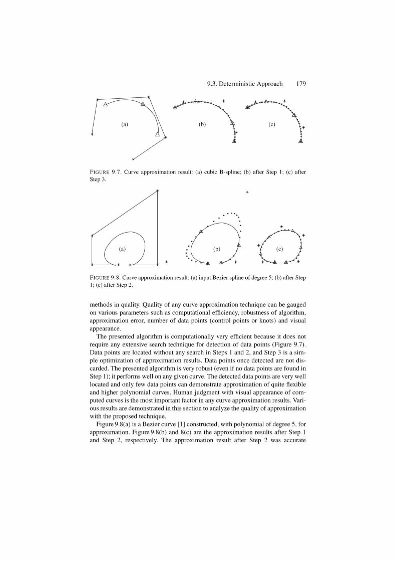
9.3. Deterministic Approach 179
(a) (b) (c)
FIGURE 9.7. Curve approximation result: (a) cubic B-spline; (b) after Step 1; (c) afterStep 3.
(a) (b) (c)
FIGURE 9.8. Curve approximation result: (a) input Bezier spline of degree 5; (b) after Step1; (c) after Step 2.
methods in quality. Quality of any curve approximation technique can be gaugedon various parameters such as computational efficiency, robustness of algorithm,approximation error, number of data points (control points or knots) and visualappearance.
The presented algorithm is computationally very efficient because it does notrequire any extensive search technique for detection of data points (Figure 9.7).Data points are located without any search in Steps 1 and 2, and Step 3 is a sim-ple optimization of approximation results. Data points once detected are not dis-carded. The presented algorithm is very robust (even if no data points are found inStep 1); it performs well on any given curve. The detected data points are very welllocated and only few data points can demonstrate approximation of quite flexibleand higher polynomial curves. Human judgment with visual appearance of com-puted curves is the most important factor in any curve approximation results. Vari-ous results are demonstrated in this section to analyze the quality of approximationwith the proposed technique.
Figure 9.8(a) is a Bezier curve [1] constructed, with polynomial of degree 5, forapproximation. Figure 9.8(b) and 8(c) are the approximation results after Step 1and Step 2, respectively. The approximation result after Step 2 was accurate
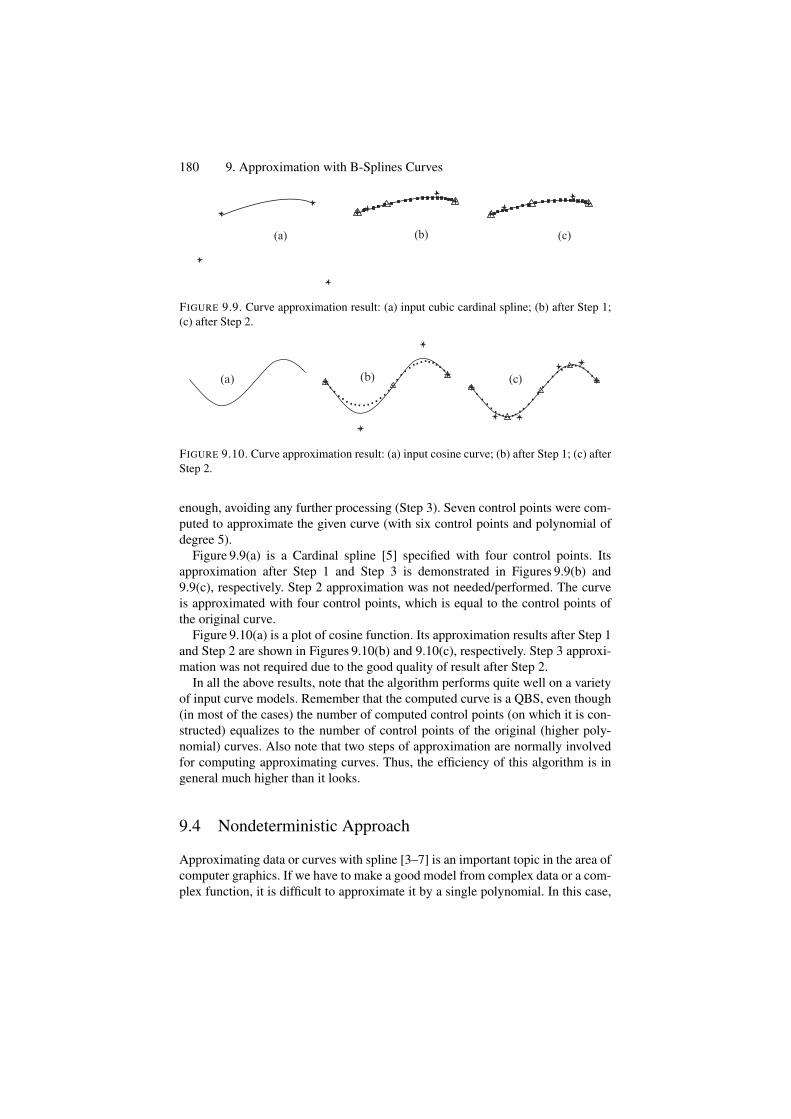
180 9. Approximation with B-Splines Curves
(a) (b) (c)
FIGURE 9.9. Curve approximation result: (a) input cubic cardinal spline; (b) after Step 1;(c) after Step 2.
(b) (c)(a)
FIGURE 9.10. Curve approximation result: (a) input cosine curve; (b) after Step 1; (c) afterStep 2.
enough, avoiding any further processing (Step 3). Seven control points were com-puted to approximate the given curve (with six control points and polynomial ofdegree 5).
Figure 9.9(a) is a Cardinal spline [5] specified with four control points. Itsapproximation after Step 1 and Step 3 is demonstrated in Figures 9.9(b) and9.9(c), respectively. Step 2 approximation was not needed/performed. The curveis approximated with four control points, which is equal to the control points ofthe original curve.
Figure 9.10(a) is a plot of cosine function. Its approximation results after Step 1and Step 2 are shown in Figures 9.10(b) and 9.10(c), respectively. Step 3 approxi-mation was not required due to the good quality of result after Step 2.
In all the above results, note that the algorithm performs quite well on a varietyof input curve models. Remember that the computed curve is a QBS, even though(in most of the cases) the number of computed control points (on which it is con-structed) equalizes to the number of control points of the original (higher poly-nomial) curves. Also note that two steps of approximation are normally involvedfor computing approximating curves. Thus, the efficiency of this algorithm is ingeneral much higher than it looks.
9.4 Nondeterministic Approach
Approximating data or curves with spline [3–7] is an important topic in the area ofcomputer graphics. If we have to make a good model from complex data or a com-plex function, it is difficult to approximate it by a single polynomial. In this case,
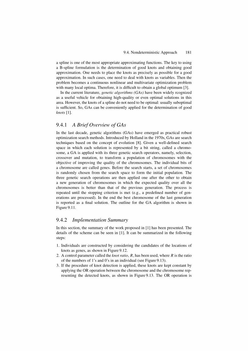
9.4. Nondeterministic Approach 181
a spline is one of the most appropriate approximating functions. The key to usinga B-spline formulation is the determination of good knots and obtaining goodapproximation. One needs to place the knots as precisely as possible for a goodapproximation. In such cases, one need to deal with knots as variables. Then theproblem becomes a continuous nonlinear and multivariate optimization problemwith many local optima. Therefore, it is difficult to obtain a global optimum [3].
In the current literature, genetic algorithms (GAs) have been widely rcognizedas a useful vehicle for obtaining high-quality or even optimal solutions in thisarea. However, the knots of a spline do not need to be optimal: usually suboptimalis sufficient. So, GAs can be conveniently applied for the determination of goodknots [1].
9.4.1 A Brief Overview of GAsIn the last decade, genetic algorithms (GAs) have emerged as practical robustoptimization search methods. Introduced by Holland in the 1970s, GAs are searchtechniques based on the concept of evolution [8]. Given a well-defined searchspace in which each solution is represented by a bit string, called a chromo-some, a GA is applied with its three genetic search operators, namely, selection,crossover and mutation, to transform a population of chromosomes with theobjective of improving the quality of the chromosomes. The individual bits ofa chromosome are called genes. Before the search starts, a set of chromosomesis randomly chosen from the search space to form the initial population. Thethree genetic search operations are then applied one after the other to obtaina new generation of chromosomes in which the expected quality over all thechromosomes is better than that of the previous generation. The process isrepeated until the stopping criterion is met (e.g., a predefined number of gen-erations are processed). In the end the best chromosome of the last generationis reported as a final solution. The outline for the GA algorithm is shown inFigure 9.11.
9.4.2 Implementation SummaryIn this section, the summary of the work proposed in [1] has been presented. Thedetails of the scheme can be seen in [1]. It can be summarized in the followingsteps:
1. Individuals are constructed by considering the candidates of the locations ofknots as genes, as shown in Figure 9.12.
2. A control parameter called the knot ratio, R, has been used, where R is the ratioof the numbers of 1’s and 0’s in an individual (see Figure 9.13).
3. If the procedure of knot detection is applied, these knots are kept constant byapplying the OR operation between the chromosome and the chromosome rep-resenting the detected knots, as shown in Figure 9.13. The OR operation is
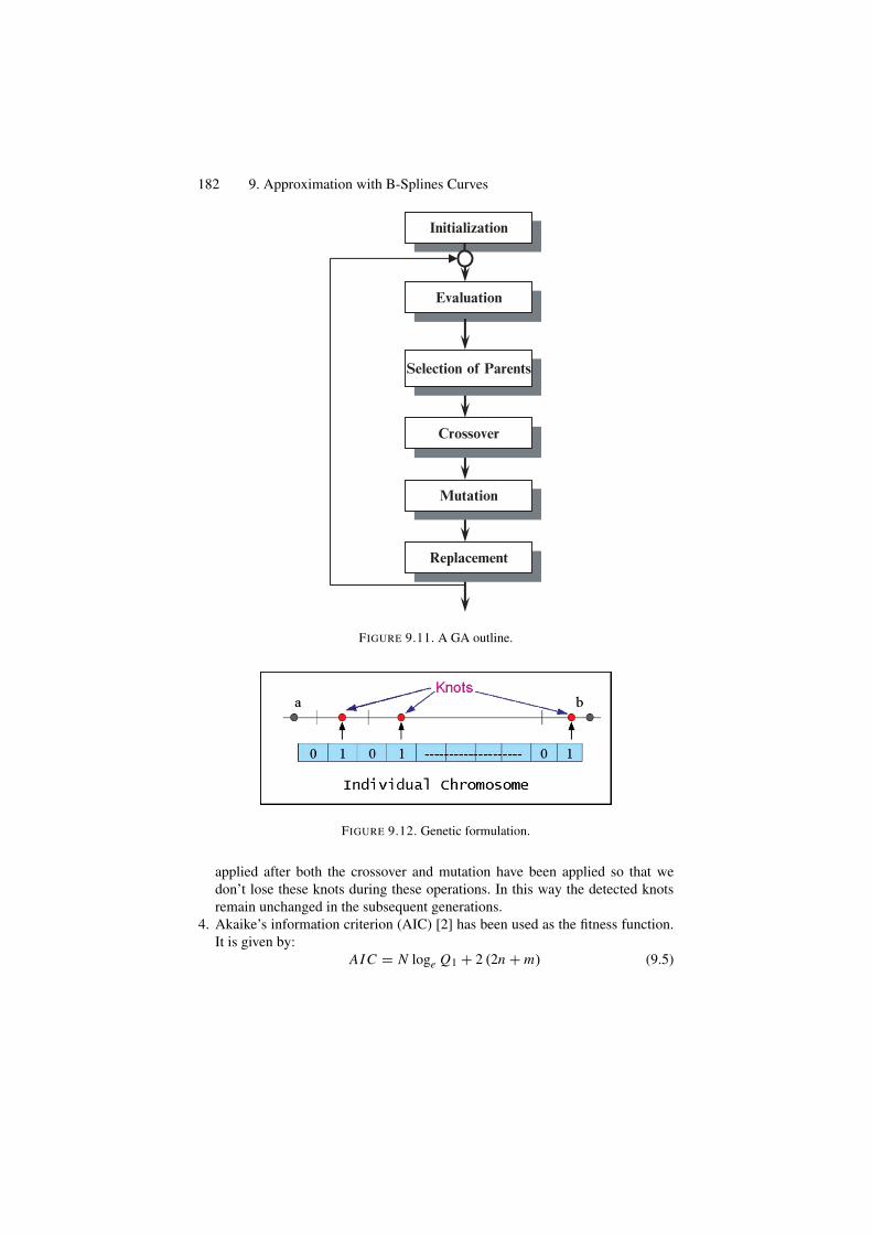
182 9. Approximation with B-Splines Curves
Initialization
Evaluation
Selection of Parents
Crossover
Mutation
Replacement
FIGURE 9.11. A GA outline.
FIGURE 9.12. Genetic formulation.
applied after both the crossover and mutation have been applied so that wedon’t lose these knots during these operations. In this way the detected knotsremain unchanged in the subsequent generations.
4. Akaike’s information criterion (AIC) [2] has been used as the fitness function.It is given by:
AI C = N loge Q1 + 2 (2n + m) (9.5)
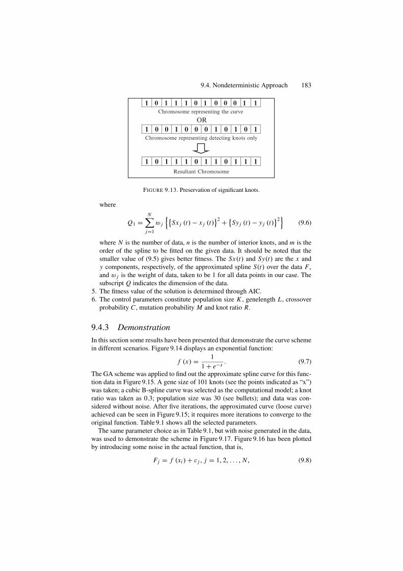
9.4. Nondeterministic Approach 183
1 0 1 1 1 0 1 0 0 0 1 1Chromosome representing the curve
OR1 0 0 1 0 0 0 1 0 1 0 1Chromosome representing detecting knots only
1 0 1 1 1 0 1 1 0 1 1 1Resultant Chromosome
FIGURE 9.13. Preservation of significant knots.
where
Q1 =N∑
j=1
w j
{{Sx j (t) − x j (t)
}2 + {Sy j (t) − y j (t)}2}
(9.6)
where N is the number of data, n is the number of interior knots, and m is theorder of the spline to be fitted on the given data. It should be noted that thesmaller value of (9.5) gives better fitness. The Sx(t) and Sy(t) are the x andy components, respectively, of the approximated spline S(t) over the data F,and w j is the weight of data, taken to be 1 for all data points in our case. Thesubscript Q indicates the dimension of the data.
5. The fitness value of the solution is determined through AIC.6. The control parameters constitute population size K , genelength L , crossover
probability C , mutation probability M and knot ratio R.
9.4.3 DemonstrationIn this section some results have been presented that demonstrate the curve schemein different scenarios. Figure 9.14 displays an exponential function:
f (x) = 11 + e−x . (9.7)
The GA scheme was applied to find out the approximate spline curve for this func-tion data in Figure 9.15. A gene size of 101 knots (see the points indicated as “x”)was taken; a cubic B-spline curve was selected as the computational model; a knotratio was taken as 0.3; population size was 30 (see bullets); and data was con-sidered without noise. After five iterations, the approximated curve (loose curve)achieved can be seen in Figure 9.15; it requires more iterations to converge to theoriginal function. Table 9.1 shows all the selected parameters.
The same parameter choice as in Table 9.1, but with noise generated in the data,was used to demonstrate the scheme in Figure 9.17. Figure 9.16 has been plottedby introducing some noise in the actual function, that is,
Fj = f (xi ) + ε j , j = 1, 2, . . . , N , (9.8)
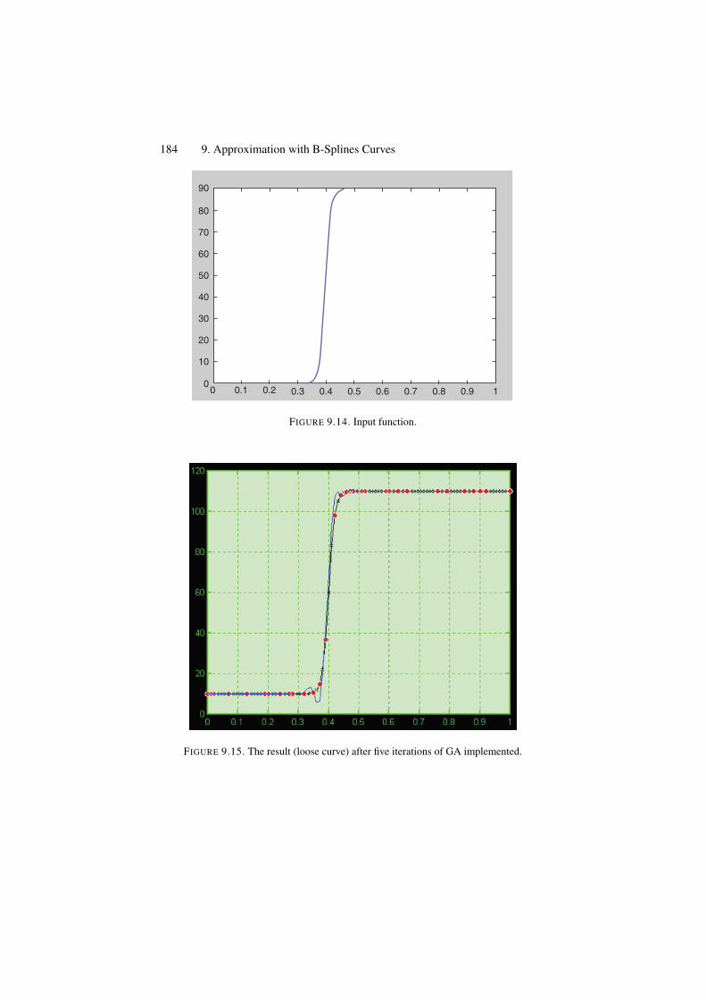
184 9. Approximation with B-Splines Curves
80
90
70
60
50
30
40
20
10
00 0.1 0.2 0.3 0.5 0.6 0.7 0.8 0.9 10.4
FIGURE 9.14. Input function.
FIGURE 9.15. The result (loose curve) after five iterations of GA implemented.
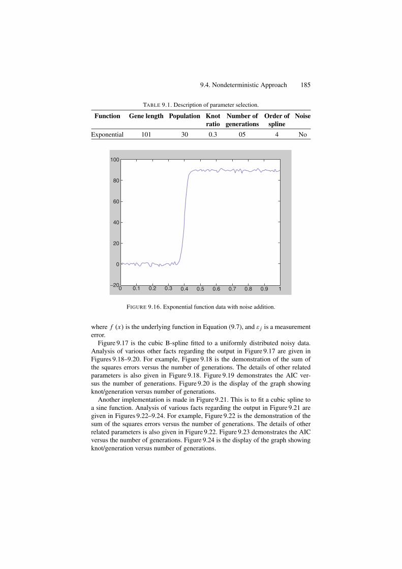
9.4. Nondeterministic Approach 185
TABLE 9.1. Description of parameter selection.
Function Gene length Population Knot Number of Order of Noiseratio generations spline
Exponential 101 30 0.3 05 4 No
100
80
60
40
20
0
0 0.1 0.2 0.3 0.4 0.5 0.6 0.7 0.8 0.9 1−20
FIGURE 9.16. Exponential function data with noise addition.
where f (x) is the underlying function in Equation (9.7), and ε j is a measurementerror.
Figure 9.17 is the cubic B-spline fitted to a uniformly distributed noisy data.Analysis of various other facts regarding the output in Figure 9.17 are given inFigures 9.18–9.20. For example, Figure 9.18 is the demonstration of the sum ofthe squares errors versus the number of generations. The details of other relatedparameters is also given in Figure 9.18. Figure 9.19 demonstrates the AIC ver-sus the number of generations. Figure 9.20 is the display of the graph showingknot/generation versus number of generations.
Another implementation is made in Figure 9.21. This is to fit a cubic spline toa sine function. Analysis of various facts regarding the output in Figure 9.21 aregiven in Figures 9.22–9.24. For example, Figure 9.22 is the demonstration of thesum of the squares errors versus the number of generations. The details of otherrelated parameters is also given in Figure 9.22. Figure 9.23 demonstrates the AICversus the number of generations. Figure 9.24 is the display of the graph showingknot/generation versus number of generations.
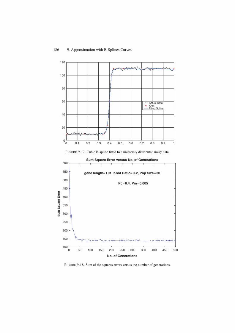
186 9. Approximation with B-Splines Curves
Actual DataKnotFitted Spline
10.8 0.90.70.60.50.40.30.20.100
20
40
60
80
100
120
FIGURE 9.17. Cubic B-spline fitted to a uniformly distributed noisy data.
0 50 100 150 200 250 300 350 400 450 500100
150
200
250
300
350
400
450
500
550
600
No. of Generations
gene length=101, Knot Ratio=0.2, Pop Size=30
Pc=0.4, Pm=0.005
Sum Square Error versus No. of Generations
Su
m S
qu
are
Err
or
FIGURE 9.18. Sum of the squares errors versus the number of generations.
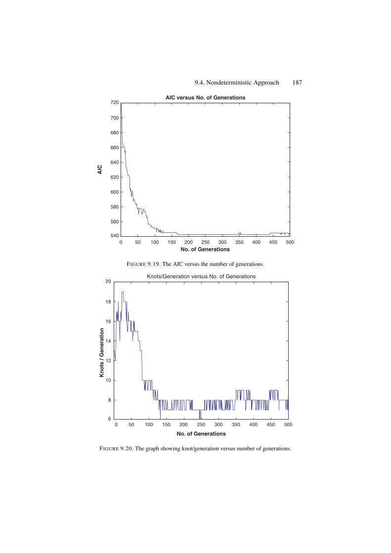
9.4. Nondeterministic Approach 187
0 50 100 150 200 250 300 350 400 450 500540
560
580
600
620
640
660
680
700
720
No. of Generations
AIC versus No. of GenerationsA
IC
FIGURE 9.19. The AIC versus the number of generations.
0 50 100 150 200 250 300 350 400 450 5006
8
10
12
14
16
18
20
No. of Generations
Knots/Generation versus No. of Generations
Kn
ots
/ G
ener
atio
n
FIGURE 9.20. The graph showing knot/generation versus number of generations.
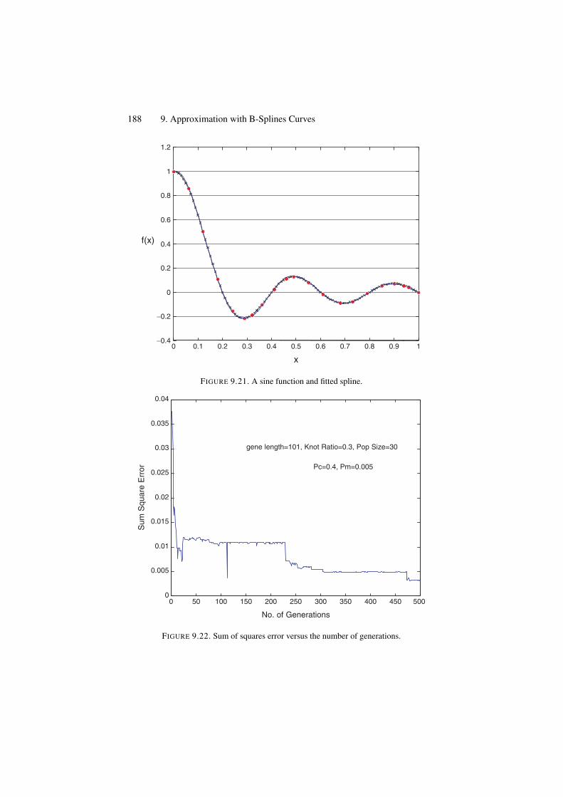
188 9. Approximation with B-Splines Curves
0 0.1 0.2 0.3 0.4 0.5 0.6 0.7 0.8 0.9 1−0.4
−0.2
0
0.2
0.4
0.6
0.8
1
1.2
f(x)
x
FIGURE 9.21. A sine function and fitted spline.
0 50 100 150 200 250 300 350 400 450 5000
0.005
0.01
0.015
0.02
0.025
0.03
0.035
0.04
No. of Generations
Sum
Squ
are
Err
or
gene length=101, Knot Ratio=0.3, Pop Size=30
Pc=0.4, Pm=0.005
FIGURE 9.22. Sum of squares error versus the number of generations.
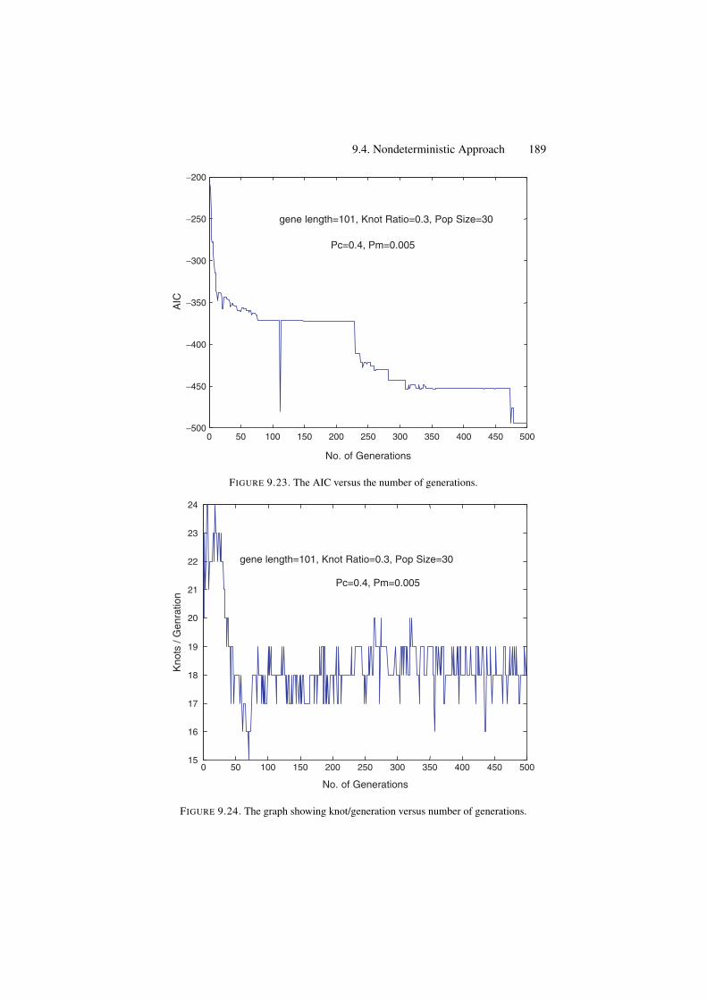
9.4. Nondeterministic Approach 189
0 50 100 150 200 250 300 350 400 450 500−500
−450
−400
−350
−300
−250
−200
No. of Generations
AIC
gene length=101, Knot Ratio=0.3, Pop Size=30
Pc=0.4, Pm=0.005
FIGURE 9.23. The AIC versus the number of generations.
0 50 100 150 200 250 300 350 400 450 50015
16
17
18
19
20
21
22
23
24
No. of Generations
Kno
ts /
Gen
ratio
n
gene length=101, Knot Ratio=0.3, Pop Size=30
Pc=0.4, Pm=0.005
FIGURE 9.24. The graph showing knot/generation versus number of generations.
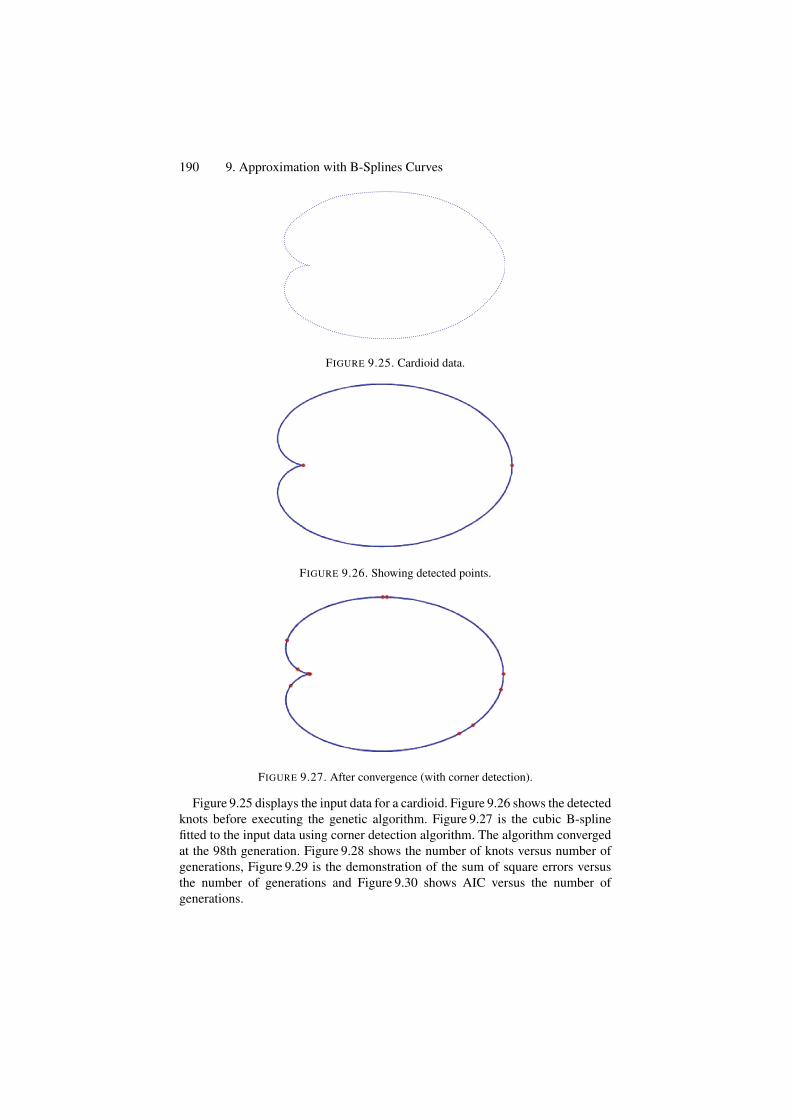
190 9. Approximation with B-Splines Curves
FIGURE 9.25. Cardioid data.
FIGURE 9.26. Showing detected points.
FIGURE 9.27. After convergence (with corner detection).
Figure 9.25 displays the input data for a cardioid. Figure 9.26 shows the detectedknots before executing the genetic algorithm. Figure 9.27 is the cubic B-splinefitted to the input data using corner detection algorithm. The algorithm convergedat the 98th generation. Figure 9.28 shows the number of knots versus number ofgenerations, Figure 9.29 is the demonstration of the sum of square errors versusthe number of generations and Figure 9.30 shows AIC versus the number ofgenerations.
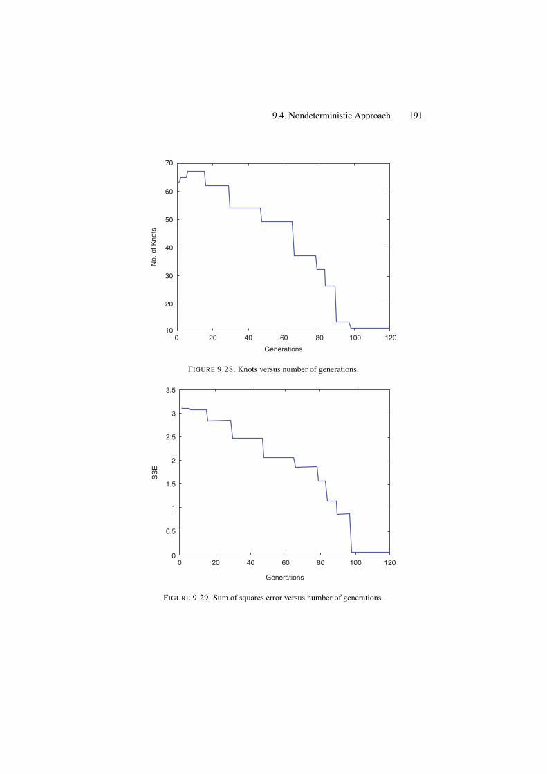
9.4. Nondeterministic Approach 191
70
60
50
40
30
20
100 20 40 60 80 100 120
Generations
No.
of K
nots
FIGURE 9.28. Knots versus number of generations.
Generations
SS
E
200
0.5
0
1
1.5
2
2.5
3
3.5
40 60 80 100 120
FIGURE 9.29. Sum of squares error versus number of generations.
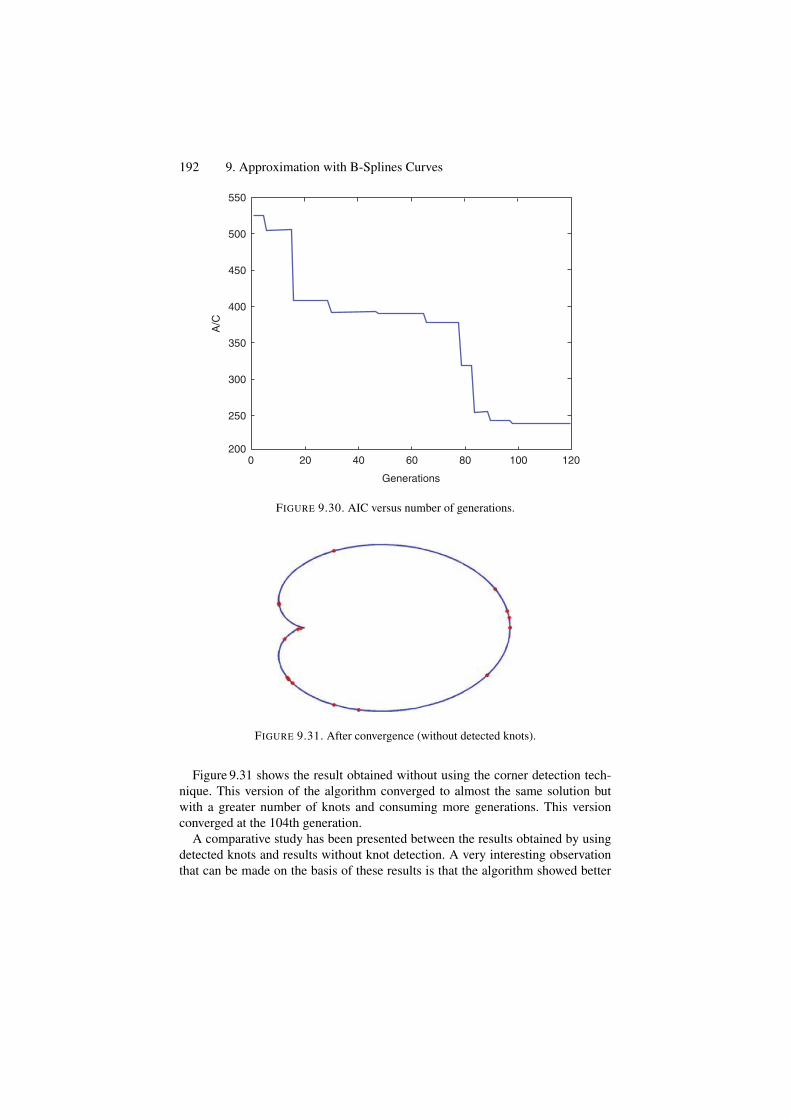
192 9. Approximation with B-Splines Curves
550
450
500
400
350
300
250
2000 20 40 60 80 100 120
Generations
A/C
FIGURE 9.30. AIC versus number of generations.
FIGURE 9.31. After convergence (without detected knots).
Figure 9.31 shows the result obtained without using the corner detection tech-nique. This version of the algorithm converged to almost the same solution butwith a greater number of knots and consuming more generations. This versionconverged at the 104th generation.
A comparative study has been presented between the results obtained by usingdetected knots and results without knot detection. A very interesting observationthat can be made on the basis of these results is that the algorithm showed better
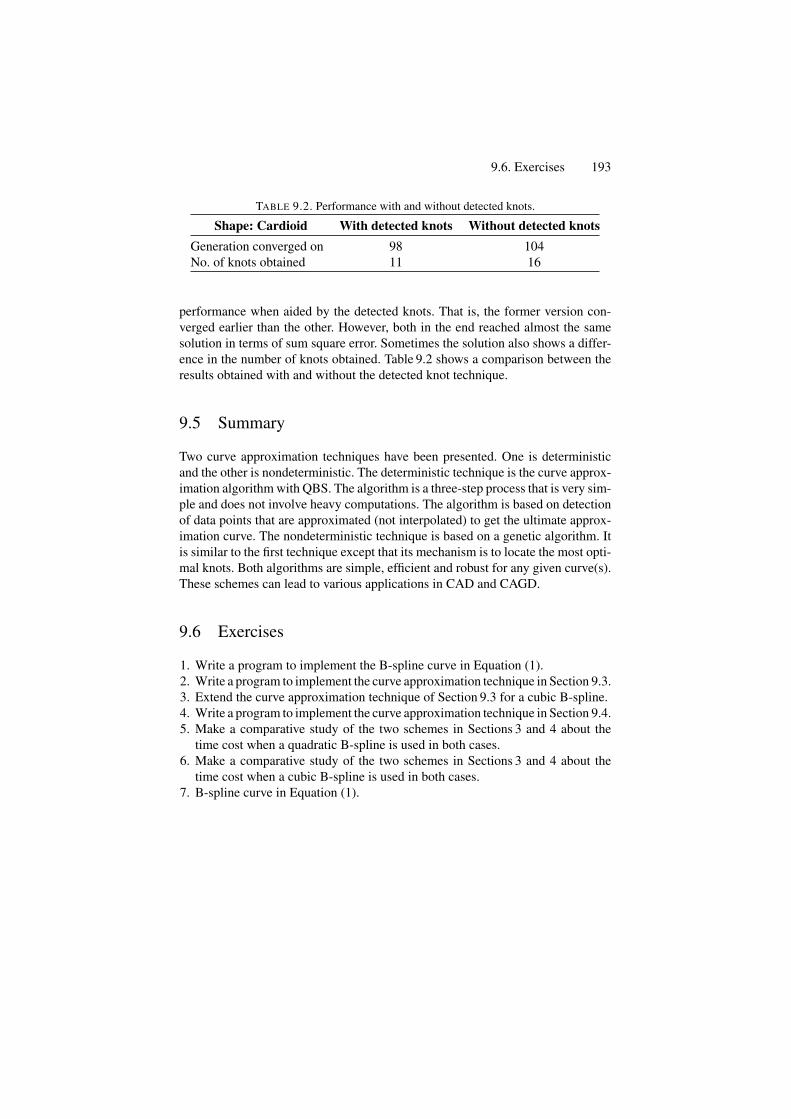
9.6. Exercises 193
TABLE 9.2. Performance with and without detected knots.
Shape: Cardioid With detected knots Without detected knotsGeneration converged on 98 104No. of knots obtained 11 16
performance when aided by the detected knots. That is, the former version con-verged earlier than the other. However, both in the end reached almost the samesolution in terms of sum square error. Sometimes the solution also shows a differ-ence in the number of knots obtained. Table 9.2 shows a comparison between theresults obtained with and without the detected knot technique.
9.5 Summary
Two curve approximation techniques have been presented. One is deterministicand the other is nondeterministic. The deterministic technique is the curve approx-imation algorithm with QBS. The algorithm is a three-step process that is very sim-ple and does not involve heavy computations. The algorithm is based on detectionof data points that are approximated (not interpolated) to get the ultimate approx-imation curve. The nondeterministic technique is based on a genetic algorithm. Itis similar to the first technique except that its mechanism is to locate the most opti-mal knots. Both algorithms are simple, efficient and robust for any given curve(s).These schemes can lead to various applications in CAD and CAGD.
9.6 Exercises
1. Write a program to implement the B-spline curve in Equation (1).2. Write a program to implement the curve approximation technique in Section 9.3.3. Extend the curve approximation technique of Section 9.3 for a cubic B-spline.4. Write a program to implement the curve approximation technique in Section 9.4.5. Make a comparative study of the two schemes in Sections 3 and 4 about the
time cost when a quadratic B-spline is used in both cases.6. Make a comparative study of the two schemes in Sections 3 and 4 about the
time cost when a cubic B-spline is used in both cases.7. B-spline curve in Equation (1).

194 9. Approximation with B-Splines Curves
References1. Bezier, P. (1974), Mathematical and practical possibilities of UNISURF. In: Barnhill.
R.E., and Riesenfeld R.F., eds. Computer Aided Geometric Design, Academic Press,New York.
2. Boehm, W. (1980), Inserting new knots into B-spline curves. Comput Aided Des 12,199–201.
3. DeBoor, C. (1977), Package for calculating with B-splines. Society for Industrial andApplied Mathematics. J Numer Anal 14(3), 441–472.
4. Farin, G. (1998), Curves and Surfaces for CAGD: A Practical Guide. Academic Press.5. Hearn, D., and Baker. M.P. (1997). Computer Graphics. Prentice-Hall, Englewood
Cliffs, NJ.6. Holzle, G.E. (1983), Knot placement for piecewise polynomial approximation of
curves. Comput Aided Des 15(5):295–296.7. Juhasz, I., and Hoffmann. M. (2001), The effect of knot modifications on the shape of
B-spline curves. J Geom Graphics 5(2), 111–119.8. Pratt, M., Goult, R., and He. L. (1993), On rational parametric curve approximation.
Comput Aided Geom Des 10(3/4):363–377.9. Razdan, A. (1999), A knot placement for B-spline curve approximation. PRISM
Publications, http://prism.asu.edu/research/data/publications/paper99 kpbsca.pdf10. Sarfraz, M., Asim, M.R., Masood. A. (2004), Capturing outlines using cubic Bezier
curves. The Proceedings of 1st IEEE International Conference on Information andCommunication Technologies: From Theory to Applications.
11. Speer, T., Kuppe, M., and Hoschek. J. (1998), Global reparametrization for curveapproximation. Comput Aided Geom Des 15, 869–877.
12. Masood, A., Sarfraz, M., and Haq, S.A. (2005), Curve approximation with quadraticB-splines, The Proceedings of IEEE International Conference on Information Visuali-sation (IV’2005)-UK, IEEE Computer Society Press, pp. 991–996.
13. Sarfraz, M, and Raza, A, (2002), Visualization of data using genetic algorithm, SoftComputing and Industry: Recent Applications, eds.: R. Roy, M. Koppen, S. Ovaska, T.Furuhashi, and F. Hoffmann, Springer-Verlag, New York, pp. 535–544.
14. Sarfraz, M, and Raza, A., (2002), Visualization of data with spline fitting: a tool witha genetic approach, The Proc. International Conference on Imaging Science, Systems,and Technology (CISST’2002), Las Vegas, Nevada, CSREA Press, pp. 99–105.
10Spirals
Abstract. Spirals are desirable for applications such as in highway route designing, robotpath planning, data-fitting problems, shape design, and curve/surface fairing in geometricmodeling. This chapter presents an efficient geometric algorithm for visualization of two-point geometric Hermite conic and arc/conic spiral segments. A comparative study is madewith those of Tschirnhausen cubic spirals.
10.1 Introduction
Manipulating and designing of curves and surfaces [1–20] is an important area ofcomputer graphics and geometric modeling. The rational quadratic Bezier curves,which are usually called the conic section curves, have been widely used for com-puter graphics applications in various industries due to their well-known propertiesand convenience for users [4, 5]. Traditionally, conic sections, when representedby NURBS [1], are in the form of a rational quadratic Bezier curve.
The curvature is one of the most important geometric concepts of curvesand surfaces. Conics have no inflection points; however, they do have curvatureextrema. Therefore, only well-chosen conic segments will have monotone curva-ture. Spirals are visually pleasing curves of monotone curvature; and they havethe advantage of not containing curvature maxima, curvature minima, inflectionpoints and singularities. Spirals are desirable for applications such as in highwayroute designing [2], robot path planning [6, 17], data-fitting problems [10], shapedesign [12], and curve/surface fairing in geometric modeling [11].
A method to create a two-point geometric Hermite planar curve by joining spiralsegments is described in [3,7,8]. The spiral segments are either spirals taken fromthe Tschirnhausen cubic curve (referred to as the T-cubic) or spirals created byjoining circular arcs to segments of the T-cubic (referred to as the arc/T-cubic)in a G3 fashion. However, it has not been possible so far to visualize the arc/T-cubic spiral on the Web due to its lot of complications in the scheme and somelimitations of Java. We solve this problem by using a conic segment instead of aT-cubic, and achieve the same level of smoothness but with a more simplified andflexible algorithm suitable for demonstration as a graphics tool.
195
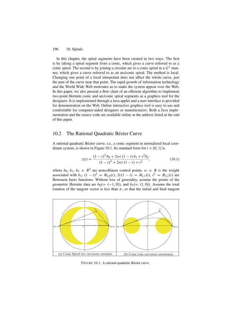
196 10. Spirals
In this chapter, the spiral segments have been created in two ways. The firstis by taking a spiral segment from a conic, which gives a curve referred to as aconic spiral. The second is by joining a circular arc to a conic spiral in a G3 man-ner, which gives a curve referred to as an arc/conic spiral. The method is local.Changing one point of a local interpolant does not affect the whole curve, justthe part of the curve near that point. The rapid growth of information technologyand the World Wide Web motivates us to make the system appear over the Web.In this paper, we also present a flow chart of an efficient algorithm to implementtwo-point Hermite conic and arc/conic spiral segments as a graphics tool for thedesigners. It is implemented through a Java applet and a user interface is providedfor demonstration on the Web. Online interactive graphics tool is easy to use andcomfortable for computer-aided designers or manufacturers. Both a Java imple-mentation and the source code are available online at the address listed at the endof this paper.
10.2 The Rational Quadratic Bezier Curve
A rational quadratic Bezier curve, i.e., a conic segment in normalized local coor-dinate system, is shown in Figure 10.1. Its standard form for t ∈ [0, 1] is
z(t) = (1 − t)2 b0 + 2wt (1 − t) b1 + t2b2
(1 − t)2 + 2wt (1 − t) + t2, (10.1)
where b0, b1, b2 ∈ R2 are noncollinear control points, w ∈ R is the weightassociated with b1, (1 − t)2 = B2,0(t), 2t (1 − t) = B2,1(t), t2 = B2,2(t) areBernstein basis functions. Without loss of generality, assume the points of thegeometric Hermite data are b0(= (−1, 0)), and b2(= (1, 0)). Assume the totalrotation of the tangent vector is less than π , so that the initial and final tangent
b0(−1,0) b0(−1,0)b2(1,0) b2(1,0)
b1b1
00
(a) Conic Spiral (no curvature extrema). (b) Conic (one curvature extremum).
FIGURE 10.1. A rational quadratic Bezier curve.
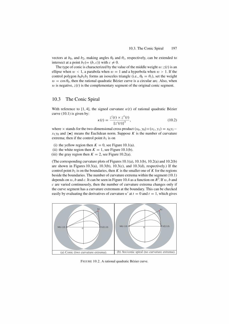
10.3. The Conic Spiral 197
vectors at b0, and b2, making angles θ0 and θ1, respectively, can be extended tointersect at a point b1(= (b, c)) with c = 0.
The type of conic is characterized by the value of the middle weight w: z(t) is anellipse when w < 1, a parabola when w = 1 and a hyperbola when w > 1. If thecontrol polygon b0b1b2 forms an isosceles triangle (i.e., θ0 = θ1), set the weightw = cos θ0, then the rational quadratic Bezier curve is a circular arc. Also, whenw is negative, z(t) is the complementary segment of the original conic segment.
10.3 The Conic Spiral
With reference to [1, 4], the signed curvature κ(t) of rational quadratic Beziercurve (10.1) is given by:
κ(t) = z′(t) × z′′(t)‖z′(t)‖3 , (10.2)
where × stands for the two-dimensional cross product (x0, y0)×(x1, y1) = x0 y1−x1 y0 and ||•|| means the Euclidean norm. Suppose K is the number of curvatureextrema; then if the control point b1 is on
(i) the yellow region then K = 0, see Figure 10.1(a).(ii) the white region then K = 1, see Figure 10.1(b).
(iii) the gray region then K = 2, see Figure 10.2(a).
(The corresponding curvature plots of Figures 10.1(a), 10.1(b), 10.2(a) and 10.2(b)are shown in Figures 10.3(a), 10.3(b), 10.3(c), and 10.3(d), respectively.) If thecontrol point b1 is on the boundaries, then K is the smaller one of K for the regionsbeside the boundaries. The number of curvature extrema within the segment (10.1)depends on w, b and c. It can be seen in Figure 10.4 as a function on R3. If w, b andc are varied continuously, then the number of curvature extrema changes only ifthe curve segment has a curvature extremum at the boundary. This can be checkedeasily by evaluating the derivatives of curvature κ ′ at t = 0 and t = 1, which gives
(a) Conic (two curvature extrema).
b1
b0(-1,0) b0(-1,0)b2(1,0) b2(1,0)
b1
(b) Arc/conic spiral (no curvature extrema).
00
FIGURE 10.2. A rational quadratic Bezier curve.
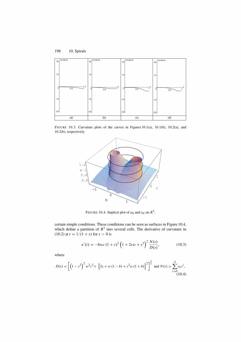
198 10. Spirals
t t t t0.5 0.5 10.5 10.5
0 0 0 0
−10
−20
10
20
−10
−20
10
20
−10
−20
10
20
−10
−20
10
20
(a) (b) (c) (d)
curvaturecurvaturecurvaturecurvature
1 1
FIGURE 10.3. Curvature plots of the curves in Figures 10.1(a), 10.1(b), 10.2(a), and10.2(b), respectively.
-10
1b -1
0
1
c0.60.81
1.2w
-10
1b
FIGURE 10.4. Implicit plot of a0 and a4 on R3.
certain simple conditions. These conditions can be seen as surfaces in Figure 10.4,which define a partition of R3 into several cells. The derivative of curvature in(10.2) at t = 1/(1 + s) for s > 0 is
κ ′(t) = −6wc (1 + s)2(
1 + 2sw + s2)2 N (s)
D(s), (10.3)
where
D(s) =[(
1 − s2)2
w2c2+{
2s + w (1 − b) + s2w (1 + b)}2] 5
2and N (s) =
4∑
i=0
ai si ,
(10.4)
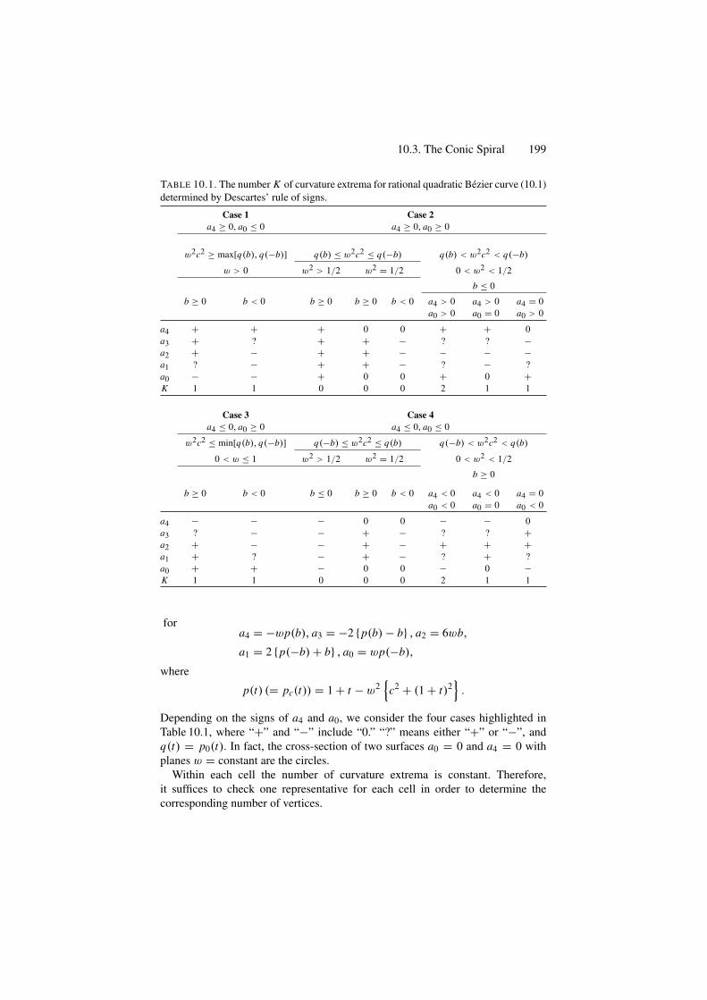
10.3. The Conic Spiral 199
TABLE 10.1. The number K of curvature extrema for rational quadratic Bezier curve (10.1)determined by Descartes’ rule of signs.
Case 1 Case 2a4 ≥ 0, a0 ≤ 0 a4 ≥ 0, a0 ≥ 0
w2c2 ≥ max[q(b), q(−b)] q(b) ≤ w2c2 ≤ q(−b) q(b) < w2c2 < q(−b)
w > 0 w2 > 1/2 w2 = 1/2 0 < w2 < 1/2
b ≤ 0
b ≥ 0 b < 0 b ≥ 0 b ≥ 0 b < 0 a4 > 0a0 > 0
a4 > 0a0 = 0
a4 = 0a0 > 0
a4 + + + 0 0 + + 0a3 + ? + + − ? ? −a2 + − + + − − − −a1 ? − + + − ? − ?a0 − − + 0 0 + 0 +K 1 1 0 0 0 2 1 1
Case 3 Case 4a4 ≤ 0, a0 ≥ 0 a4 ≤ 0, a0 ≤ 0
w2c2 ≤ min[q(b), q(−b)] q(−b) ≤ w2c2 ≤ q(b) q(−b) < w2c2 < q(b)
0 < w ≤ 1 w2 > 1/2 w2 = 1/2 0 < w2 < 1/2
b ≥ 0
b ≥ 0 b < 0 b ≤ 0 b ≥ 0 b < 0 a4 < 0 a4 < 0 a4 = 0a0 < 0 a0 = 0 a0 < 0
a4 − − − 0 0 − − 0a3 ? − − + − ? ? +a2 + − − + − + + +a1 + ? − + − ? + ?a0 + + − 0 0 − 0 −K 1 1 0 0 0 2 1 1
fora4 = −wp(b), a3 = −2 {p(b) − b} , a2 = 6wb,
a1 = 2 {p(−b) + b} , a0 = wp(−b),
where
p(t) (= pc(t)) = 1 + t − w2{
c2 + (1 + t)2}
.
Depending on the signs of a4 and a0, we consider the four cases highlighted inTable 10.1, where “+” and “−” include “0.” “?” means either “+” or “−”, andq(t) = p0(t). In fact, the cross-section of two surfaces a0 = 0 and a4 = 0 withplanes w = constant are the circles.
Within each cell the number of curvature extrema is constant. Therefore,it suffices to check one representative for each cell in order to determine thecorresponding number of vertices.
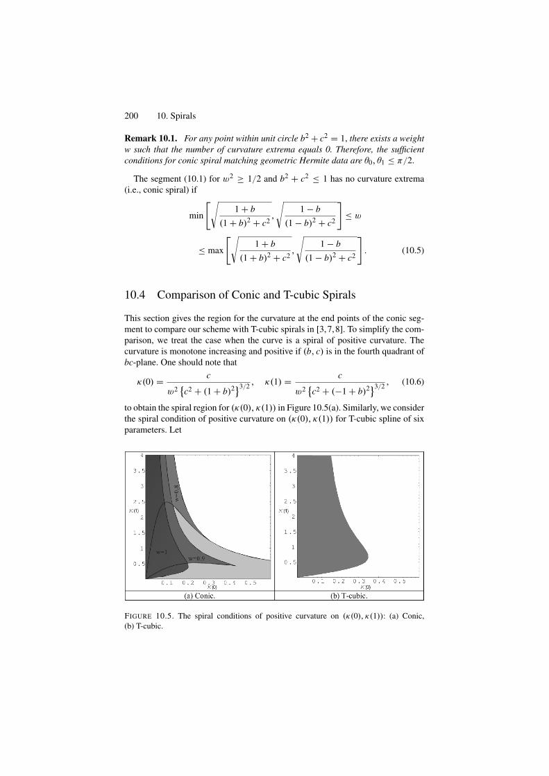
200 10. Spirals
Remark 10.1. For any point within unit circle b2 + c2 = 1, there exists a weightw such that the number of curvature extrema equals 0. Therefore, the sufficientconditions for conic spiral matching geometric Hermite data are θ0, θ1 ≤ π/2.
The segment (10.1) for w2 ≥ 1/2 and b2 + c2 ≤ 1 has no curvature extrema(i.e., conic spiral) if
min
[√1 + b
(1 + b)2 + c2,
√1 − b
(1 − b)2 + c2
]
≤ w
≤ max
[√1 + b
(1 + b)2 + c2,
√1 − b
(1 − b)2 + c2
]
. (10.5)
10.4 Comparison of Conic and T-cubic Spirals
This section gives the region for the curvature at the end points of the conic seg-ment to compare our scheme with T-cubic spirals in [3,7,8]. To simplify the com-parison, we treat the case when the curve is a spiral of positive curvature. Thecurvature is monotone increasing and positive if (b, c) is in the fourth quadrant ofbc-plane. One should note that
κ(0) = c
w2{c2 + (1 + b)2}3/2 , κ(1) = c
w2{c2 + (−1 + b)2}3/2 , (10.6)
to obtain the spiral region for (κ(0), κ(1)) in Figure 10.5(a). Similarly, we considerthe spiral condition of positive curvature on (κ(0), κ(1)) for T-cubic spline of sixparameters. Let
FIGURE 10.5. The spiral conditions of positive curvature on (κ(0), κ(1)): (a) Conic,(b) T-cubic.
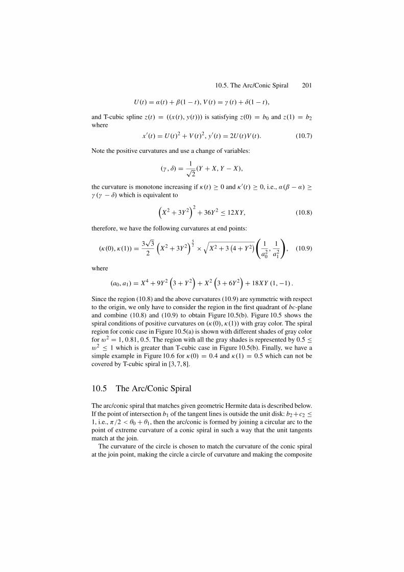
10.5. The Arc/Conic Spiral 201
U (t) = α(t) + β(1 − t), V (t) = γ (t) + δ(1 − t),
and T-cubic spline z(t) = ((x(t), y(t))) is satisfying z(0) = b0 and z(1) = b2where
x ′(t) = U (t)2 + V (t)2, y′(t) = 2U (t)V (t). (10.7)
Note the positive curvatures and use a change of variables:
(γ, δ) = 1√2(Y + X, Y − X),
the curvature is monotone increasing if κ(t) ≥ 0 and κ ′(t) ≥ 0, i.e., α(β − α) ≥γ (γ − δ) which is equivalent to
(X2 + 3Y 2
)2 + 36Y 2 ≤ 12XY, (10.8)
therefore, we have the following curvatures at end points:
(κ(0), κ(1)) = 3√
32
(X2 + 3Y 2
) 52 ×
√X2 + 3
(4 + Y 2
)(
1a2
0,
1a2
1
)
, (10.9)
where
(a0, a1) = X4 + 9Y 2(
3 + Y 2)
+ X2(
3 + 6Y 2)
+ 18XY (1,−1) .
Since the region (10.8) and the above curvatures (10.9) are symmetric with respectto the origin, we only have to consider the region in the first quadrant of bc-planeand combine (10.8) and (10.9) to obtain Figure 10.5(b). Figure 10.5 shows thespiral conditions of positive curvatures on (κ(0), κ(1)) with gray color. The spiralregion for conic case in Figure 10.5(a) is shown with different shades of gray colorfor w2 = 1, 0.81, 0.5. The region with all the gray shades is represented by 0.5 ≤w2 ≤ 1 which is greater than T-cubic case in Figure 10.5(b). Finally, we have asimple example in Figure 10.6 for κ(0) = 0.4 and κ(1) = 0.5 which can not becovered by T-cubic spiral in [3, 7, 8].
10.5 The Arc/Conic Spiral
The arc/conic spiral that matches given geometric Hermite data is described below.If the point of intersection b1 of the tangent lines is outside the unit disk: b2 +c2 ≤1, i.e., π/2 < θ0 + θ1, then the arc/conic is formed by joining a circular arc to thepoint of extreme curvature of a conic spiral in such a way that the unit tangentsmatch at the join.
The curvature of the circle is chosen to match the curvature of the conic spiralat the join point, making the circle a circle of curvature and making the composite
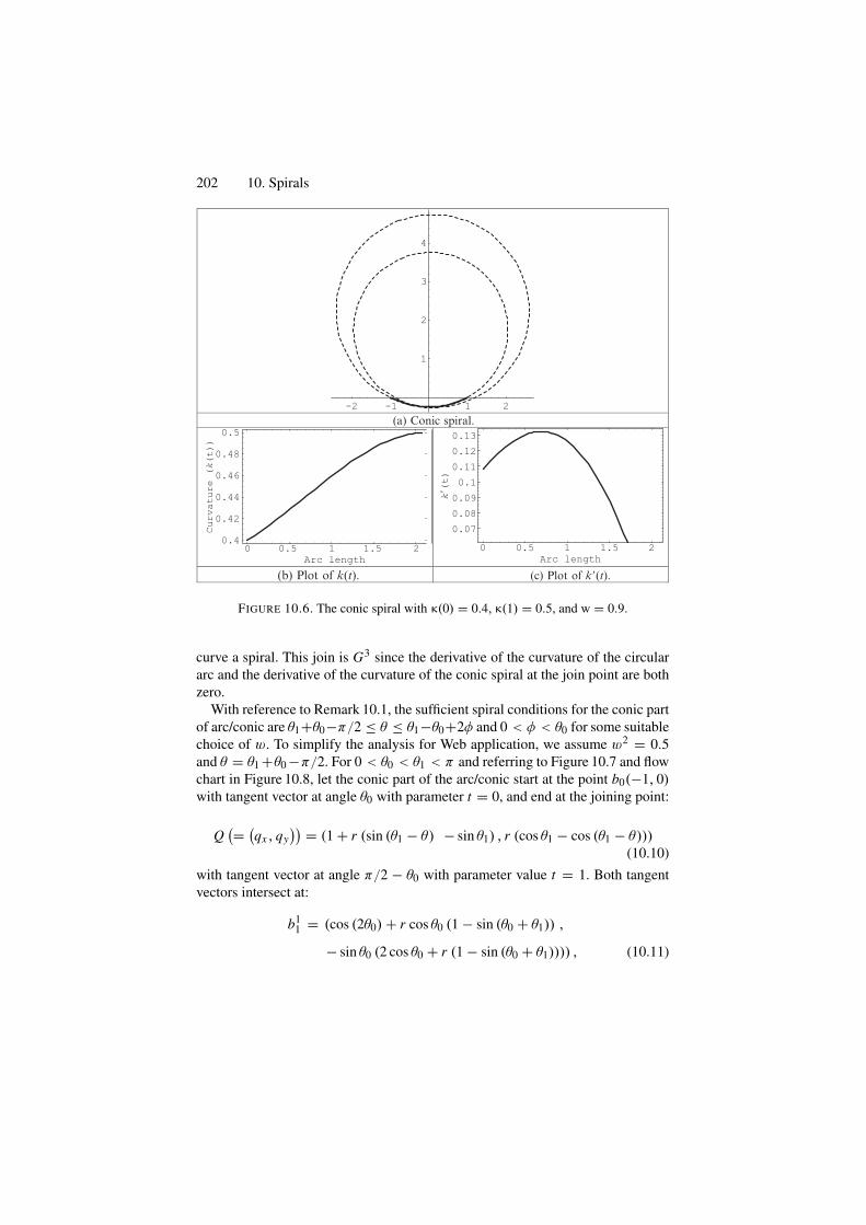
202 10. Spirals
-2 -1 1 2
1
2
3
4
(a) Conic spiral.
0 0.5 1 1.5 2Arc length
0.40.420.440.460.480.5
Curv
atur
e (k
(t))
k�(t
)
0 0.5 1 1.5 2Arc length
0.070.080.090.1
0.110.120.13
(b) Plot of k(t). (c) Plot of k�(t).
FIGURE 10.6. The conic spiral with κ(0) = 0.4, κ(1) = 0.5, and w = 0.9.
curve a spiral. This join is G3 since the derivative of the curvature of the circulararc and the derivative of the curvature of the conic spiral at the join point are bothzero.
With reference to Remark 10.1, the sufficient spiral conditions for the conic partof arc/conic are θ1+θ0−π/2 ≤ θ ≤ θ1−θ0+2φ and 0 < φ < θ0 for some suitablechoice of w. To simplify the analysis for Web application, we assume w2 = 0.5and θ = θ1 +θ0 −π/2. For 0 < θ0 < θ1 < π and referring to Figure 10.7 and flowchart in Figure 10.8, let the conic part of the arc/conic start at the point b0(−1, 0)with tangent vector at angle θ0 with parameter t = 0, and end at the joining point:
Q(= (qx , qy
)) = (1 + r (sin (θ1 − θ) − sin θ1) , r (cos θ1 − cos (θ1 − θ)))(10.10)
with tangent vector at angle π/2 − θ0 with parameter value t = 1. Both tangentvectors intersect at:
b11 = (cos (2θ0) + r cos θ0 (1 − sin (θ0 + θ1)) ,
− sin θ0 (2 cos θ0 + r (1 − sin (θ0 + θ1)))) , (10.11)

10.5. The Arc/Conic Spiral 203
θ0
θ
φ θ
Q
P
r
r
b1
b12
b11
b0 (−1,0) b2 (1,0)(0,0)
1
φ+θ1−θ
FIGURE 10.7. Arc/conic spiral.
Let the arc part of the arc/conic with radius
r = 1sin (θ0 + θ1) (sin (θ0 + θ1) − 1)
{sin (2θ0 + θ1)
+√
4 − 3 cos2 θ0 − 4 cos θ1 sin θ0 − cos θ0 − sin θ1
}, (10.12)
starting from the point Q with tangent vector at angle π/2 − θ0, sweep throughan angle θ and end at the point b2(1, 0) with tangent vector at angle π + θ1. Bothtangent vectors intersect at
b21 =
(m0qx − m1 − qy, m0m1 (qx − 1) − m1qy
)
m0 − m1(10.13)
wherem0 = tan
(π
2− θ0
), m1 = tan(π + θ1).
Then quadratic Bezier curve (10.1) is the desired arc for b1 = b21, w = cos
(θ2
).
A simple example of an arc/conic spiral segment is shown in Figure 10.2(b) withcorresponding curvature plot in Figure 10.3(d).
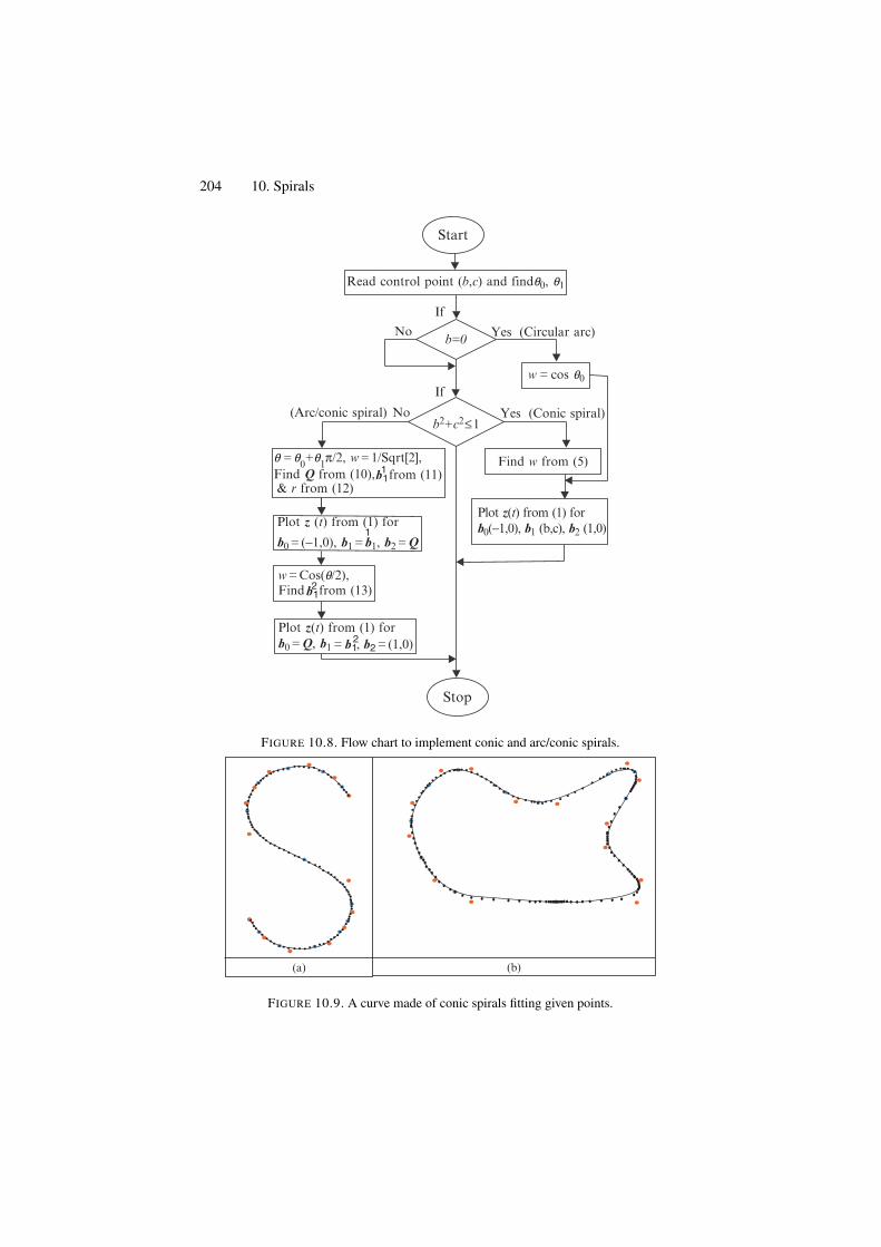
204 10. Spirals
Start
Stop
Read control point (b,c) and findq0, q1
b=0
If
b2+c2≤1
Yes (Circular arc)No
w = cos q0
q = q0+q1π/2, w = 1/Sqrt[2],
Yes (Conic spiral)(Arc/conic spiral) No
If
Find w from (5)
Plot z(t) from (1) forb0(−1,0), b1 (b,c), b2 (1,0)
Find Q from (10),& r from (12)
from (11)
Plot z (t) from (1) for
b0 = (−1,0), b1 = b1, b2 = Q1
b11
Find from (13)w = Cos(q/2),
Plot z(t) from (1) for
b12
b0 = Q, b1 = , b2 = (1,0)b12
FIGURE 10.8. Flow chart to implement conic and arc/conic spirals.
(b)(a)
FIGURE 10.9. A curve made of conic spirals fitting given points.
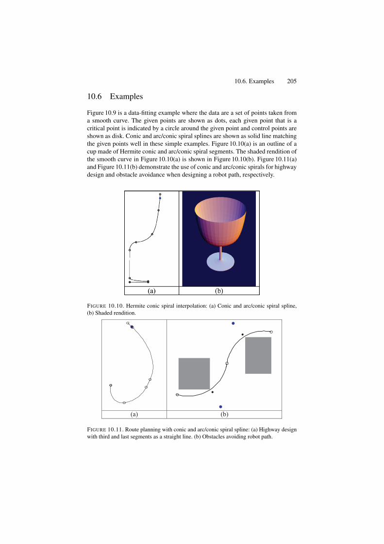
10.6. Examples 205
10.6 Examples
Figure 10.9 is a data-fitting example where the data are a set of points taken froma smooth curve. The given points are shown as dots, each given point that is acritical point is indicated by a circle around the given point and control points areshown as disk. Conic and arc/conic spiral splines are shown as solid line matchingthe given points well in these simple examples. Figure 10.10(a) is an outline of acup made of Hermite conic and arc/conic spiral segments. The shaded rendition ofthe smooth curve in Figure 10.10(a) is shown in Figure 10.10(b). Figure 10.11(a)and Figure 10.11(b) demonstrate the use of conic and arc/conic spirals for highwaydesign and obstacle avoidance when designing a robot path, respectively.
FIGURE 10.10. Hermite conic spiral interpolation: (a) Conic and arc/conic spiral spline,(b) Shaded rendition.
(a) (b)
FIGURE 10.11. Route planning with conic and arc/conic spiral spline: (a) Highway designwith third and last segments as a straight line. (b) Obstacles avoiding robot path.
206 10. Spirals
10.7 Limitations
Although both arc/conic and T/cubic spirals have G3 continuity internally, thejoining of neighboring pairs of spirals gives a curve that has only tangent conti-nuity. Meek and Walton [9] presented a method for C-shaped interpolating curvemade of one or two conic spiral segments. This curve is curvature continuouswith monotone curvature, but this fairness is achieved at the cost of nonflexibilityand inconvenience of use in practical applications. For example, in their methodthe angle between tangents at end points must be less than π/2, where as in ourarc/conic case it is less than π . Their method is also restricted for the case when thesign of curvatures at end points are same and nonzero, so user has to compromiseon tangent continuity to interpolate an S-shaped curve. Further, their C-shapedcurve with one or two spiral segments cannot cover the entire region, and thereforethe examination of reachable regions for a designer may be confusing to developthe two curves separately.
10.8 Summary
An efficient geometric algorithm, for visualization of two-point geometric Hermiteconic and arc/conic spiral segments, has been presented in this chapter. A compar-ative study is made with those of Tschirnhausen cubic spirals. Spirals are desirablefor applications such as in highway route designing, robot path planning, data-fitting problems, shape design, and curve/surface fairing in geometric modeling.
10.9 Exercises
1. What is a spiral?2. What are the main applications of spiral curves?3. Implement the spiral algorithms in this chapter.
References1. Farin, G. (1995), NURB Curves and Surfaces. A.K Peters, 1995.2. Gibreel, G.M., Easa, S.M., Hassan, Y., and El-Dimeery, I.A. (1999), State of the art of
highway geometric design consistency. ASCE J Transport Eng 125(4), 305–313.3. Habib, Z., and Sakai, M. (2002), T-cubic and arc/T-cubic spirals for Web-based visual-
ization of planar data. The Proceedings of the Fourth IEEE Workshop on Informationand Computer Science: Internet Computing (WICS’2002), KFUPM, Saudi Arabia,IEEE Computer Society Chapter, pp. 267–278.
4. Habib, Z., and Sakai, M. (2005), Conic spiral spline, International Conference onGeometric Modeling, Visualization & Graphics, JCIS, pp. 1653–1656.
5. Habib, Z., Sarfraz, M., and Sakai, M. (2005), Rational cubic spline interpolation withshape control. Comput Graphics, Elsevier Science, 29(4), 594–605.
References 207
6. Liang, T., Liu, J., Hung, G., and Chang, Y. (2005), Practical and flexible path planningfor carlike mobile robot using maximal-curvature cubic spiral. Robot Autonomous Sys52, 312–335.
7. Meek, D.S. (2002), Coaxing a planar curve to comply. J Computational Appl Math140, 599–618.
8. Meek, D.S., and Walton, D.J. (1997), Hermite interpolation with Tschirnhausen cubicspirals. Comput Aided Geom Des 14, 619–633.
9. Meek, D.S., and Walton, D.J. (2002), Planar G2 Hermite interpolation with some fair,C-shaped curves. J Computational Appl Math 139, 141–161.
10. Sarfraz, M. (2003), Optimal curve fitting to digital data. Int J WSCG 11(1), 128–135.11. Sarfraz, M., Ed. (2004), Geometric Modeling: Techniques, Applications, Systems and
Tools, Kluwer, Netherlands.12. Sarfraz, M., & Razzak, M. (2003), A Web-based system to capture outlines of Arabic
fonts. Int J Information Sci, Elsevier Science, 150(3–4), 177–193.13. Sarfraz, M., Raza, S.A., and Baig, M.H. (2005), computing optimized curves with
NURBS using evolutionary intelligence, Lecture Notes in Computer Science, Vol.3480: Computational Science and Its Applications, eds.: Gervasi, O., Gavrilova, M.L.,Kumar, V., Lagana, A., Lee, H.P., Mun, Y., Taniar, D., Springer-Verlag, New York,pp. 806–815.
14. Sarfraz, M. (2004), A rational spline with point tension: an alternative to NURBS ofDegree Three, In: Geometric Modeling: Techniques, Applications, Systems and Tools,Ed.: M. Sarfraz, Kluwer, pp. 131–148.
15. Sarfraz, M. (2004), Representing shapes by fitting data using an evolutionaryapproach, Int J Comput Aided Des Applications, 1(1–4), 179–186.
16. Sarfraz, M. (2003), Weighted Nu splines: an alternative to NURBS, In: Advances inGeometric Modeling, Ed.: M. Sarfraz, John Wiley, New York, pp. 81–95.
17. Yongguo, M., Yung-Hsiang, L., Charlie, H., and George, L. (2004), Energy-efficientmotion planning for mobile robots. The Proceedings IEEE International Conferenceon Robotics and Automation, IEEE Computer Society Press, pp. 4344–4349.
18. Sarfraz, M. and Khan, M. A. (2004), An automatic algorithm for approximatingboundary of bitmap characters, In: Future Generation Computer Systems, ElsevierScience, 20, 1327–1336.
19. Sarfraz, M. (2004), Some algorithms for curve design and automatic outline capturingof images, Int J Image Graphics, World Scientific, 4(2), 301–324.
20. Sarfraz, M. (2004), Weighted Nu splines with local support basis functions, Interna-tional J Comput Graphics, Elsevier Science, 28(4), 539–549.
21. Habib, Z., and Sakai, M. (2005), Web-based visualization of conic and arc/conicspirals, Int J Comput Graphics CAD / CAM, 1(1), 16–26.
11Corner Detection for CurveSegmentation
Abstract. Corners in digital images give important clues for shape representation andanalysis. Corner points represent important features of an object that may be useful atsubsequent levels of processing. Corners are robust features in the sense that they pro-vide important information regarding objects under translation, rotation and scale change.If the corner points are identified properly, a shape can be represented in an efficient andcompact way with sufficient accuracy in many shape analysis problems. Shape representa-tion and image interpretation depends, in most cases, on how correctly and efficiently thecorner points are located. Specifically, in the area of vectorizing planar images, contoursegmentation is very often managed by locating the exact corner points. This leads to thepiecewise solution of the problem.
11.1 Introduction
Corners in digital images give important clues for shape representation and analy-sis. Since dominant information regarding shape is usually available at the cor-ners, they provide important features for object recognition, shape representationand image interpretation. Corners are robust features in the sense that they pro-vide important information regarding objects under translation, rotation and scalechange. If the corner points are identified properly, a shape can be representedin an efficient and compact way with sufficient accuracy in many shape analysisproblem.
Corner points represent important features of an object that may be useful at asubsequent level of computer vision. Guru et al. [12] state that information abouta shape is concentrated at the corners and that corners practically prove to bedescriptive primitives in shape representation and image interpretation. Asada andBrady [2] insist that these points play a dominant role in shape perception byhumans. Attneave [3] proposed that information along a visual contour is concen-trated in the regions of high magnitude of curvature. Corner points are used invarious computer vision, computer graphics, and pattern recognition applications.It can be used as a step in document image analysis, such as chart and diagram
209
210 11. Corner Detection for Curve Segmentation
processing [15], and is also important from the view point of understanding humanperception of objects [3]. Corner points play a crucial role in decomposing ordescribing a curve [1]. They are also used in scale space theory [8, 18], imagerepresentation [5], stereo vision [9, 33], motion tracking [10, 34], image match-ing [29, 32], building 2D mosaics [35] and preprocessing phase of outline captur-ing systems [26, 27].
Corner detection schemes can be broadly divided into two categories based ontheir applications:
• binary (suitable for binary images) and• gray level (suitable for gray level images)
Corner detection approaches for binary images usually involve segmentingthe image into regions and extracting boundaries from those regions that containthem. The techniques for gray-level images can be categorized into two classes:(a) template based and (b) gradient based. The template-based technique utilizescorrelation between a subimage and a template of a given angle. A corner pointis selected by finding the maximum of the correlation output. Gradient-basedtechniques require computing the curvature of an edge that passes through aneighborhood in a gray-level image.
Many corner detection algorithms have been proposed which can be broadlydivided into two parts. One is to detect corner points from grayscale images [13,16, 19, 30] and another relates to boundary-based corner detection [4, 6, 11, 13,17, 20, 24, 28, 38]. This chapter mainly deals with techniques adopted for laterapproach.
11.2 Basic Formulation
Visually, corners are the endpoints of straight-line segments of polygonal shapes.But it is difficult and complicated to determine corners in case of nonparametriccurves as well as outlines of natural objects especially when the noise is carried.In general, corners represent significant features of an object that human beingswould perceive as the meaningful points. Detection of these points is not an easyjob since accuracy of detected corners is gauged purely by human judgment and nostandard definition/criteria exists. In order to compute the corners, it is importantto give them some mathematical representation. In the literature, different authorshave described them in different ways. Abe and Kandonaga [1] described cornersas local maxima points. They proposed a method for decomposing curves intostraight segments and curved arcs, based on the slope at each point. Guru et al. [12]smoothed the boundary curve and found a difference at each curve point calleda “cornerity index.” The larger values of the cornerity index were taken to becorners.
Rosenfeld and Johnston [23] took curvature maxima points using k-cosine ascorners. Rosenfeld and Weszka [24] proposed a modification of [23] in which
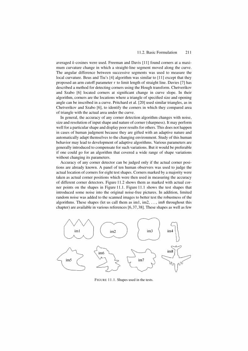
11.2. Basic Formulation 211
averaged k-cosines were used. Freeman and Davis [11] found corners at a maxi-mum curvature change in which a straight-line segment moved along the curve.The angular difference between successive segments was used to measure thelocal curvature. Beus and Tiu’s [4] algorithm was similar to [11] except that theyproposed an arm cutoff parameter τ to limit length of straight line. Davies [7] hasdescribed a method for detecting corners using the Hough transform. Chetverikovand Szabo [6] located corners at significant change in curve slope. In theiralgorithm, corners are the locations where a triangle of specified size and openingangle can be inscribed in a curve. Pritchard et al. [20] used similar triangles, as inChetverikov and Szabo [6], to identify the corners in which they compared areaof triangle with the actual area under the curve.
In general, the accuracy of any corner detection algorithm changes with noise,size and resolution of input shape and nature of corner (sharpness). It may performwell for a particular shape and display poor results for others. This does not happenin cases of human judgment because they are gifted with an adaptive nature andautomatically adapt themselves to the changing environment. Study of this humanbehavior may lead to development of adaptive algorithms. Various parameters aregenerally introduced to compensate for such variations. But it would be preferableif one could go for an algorithm that covered a wide range of shape variationswithout changing its parameters.
Accuracy of any corner detector can be judged only if the actual corner posi-tions are already known. A panel of ten human observers was used to judge theactual location of corners for eight test shapes. Corners marked by a majority weretaken as actual corner positions which were then used in measuring the accuracyof different corner detectors. Figure 11.2 shows them as marked with actual cor-ner points on the shapes in Figure 11.1. Figure 11.1 shows the test shapes thatintroduced some noise into the original noise-free pictures. In addition, limitedrandom noise was added to the scanned images to better test the robustness of thealgorithms. These shapes (let us call them as im1, im2, . . . , im8 throughout thischapter) are available in various references [6,37,38]. These shapes as well as few
FIGURE 11.1. Shapes used in the tests.
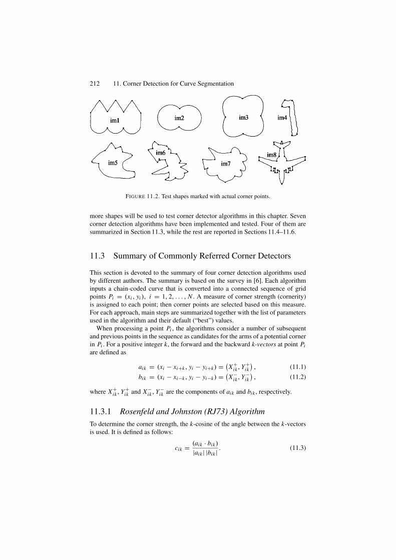
212 11. Corner Detection for Curve Segmentation
FIGURE 11.2. Test shapes marked with actual corner points.
more shapes will be used to test corner detector algorithms in this chapter. Sevencorner detection algorithms have been implemented and tested. Four of them aresummarized in Section 11.3, while the rest are reported in Sections 11.4–11.6.
11.3 Summary of Commonly Referred Corner Detectors
This section is devoted to the summary of four corner detection algorithms usedby different authors. The summary is based on the survey in [6]. Each algorithminputs a chain-coded curve that is converted into a connected sequence of gridpoints Pi = (xi , yi ), i = 1, 2, . . . , N . A measure of corner strength (cornerity)is assigned to each point; then corner points are selected based on this measure.For each approach, main steps are summarized together with the list of parametersused in the algorithm and their default (“best”) values.
When processing a point Pi , the algorithms consider a number of subsequentand previous points in the sequence as candidates for the arms of a potential cornerin Pi . For a positive integer k, the forward and the backward k-vectors at point Piare defined as
aik = (xi − xi+k, yi − yi+k) = (X+ik, Y +
ik), (11.1)
bik = (xi − xi−k, yi − yi−k) = (X−ik, Y −
ik), (11.2)
where X+ik, Y +
ik and X−ik, Y −
ik are the components of aik and bik , respectively.
11.3.1 Rosenfeld and Johnston (RJ73) AlgorithmTo determine the corner strength, the k-cosine of the angle between the k-vectorsis used. It is defined as follows:
cik = (aik · bik)
|aik | |bik | . (11.3)
11.3. Summary of Commonly Referred Corner Detectors 213
where aik and bik are explained in Equations (11.1) and (11.2), respectively. Theselection procedure for the corner points is as follows. Starting from m = k N ,k is decremented until cik stops to increase. That is:
cim < ci,m−1 < . . . < cin ≮ ci, n − 1.
Then k = n is selected as the best value for the i th point. A corner is indicated ini if cin > c jp for all j such that |i − j | ≤ n/2, where p is the best value of k forthe j th point. The single parameter κ specifies the maximum considered value ofk as a fraction of the total number of curve points N . This limits the length of anarm at κ N . The default value is taken as κ = 0.05.
For more details of the algorithm, the reader is referred to [23]. Demonstrationof the algorithm, for the shapes im1, im2, . . . , im8, is made in Figure 11.24.The choice of the selected parameters, for these figures, can be seen inTable 11.2. The “D” in Table 11.2 is meant for the default values; the deviationsfrom the “D” are shown otherwise. The proposed algorithm yields reasonableresults at the shown values for all the eight shapes. Points not well located areindicated with arrows.
11.3.2 Rosenfeld and Weszka (RW75) AlgorithmTo determine the corner strength, the averaged k-cosine of the angle between thek-vectors is used, which is defined as follows:
cik =
⎧⎪⎪⎪⎨
⎪⎪⎪⎩
2k+2
k∑
t=k/2cit , if k is even,
2k+3
k∑
t=(k−1)/2cit , if k is odd,
where cit are given by Equation (11.3). The selection procedure for the cornerpoints is the same as in RJ73, but it is performed for cik . Similarly, the choice ofparameter is also same as in RJ73, with the same default value κ = 0.05.
For more details of the algorithm, the reader is referred to [24]. Demonstrationof the algorithm, for the shapes im1, im2, . . . , im8, is made in Figure 11.25. Thechoice of the selected parameters, for these figures, can be seen in Table 11.2.The “D” in Table 11.2 is meant for the default values; the deviations fromthe “D” are shown otherwise. The proposed algorithm yields reasonable resultsat the shown values for all the eight shapes. Points not well located are indicatedwith arrows.
11.3.3 Freeman and Davis (FD77) AlgorithmTo determine the corner strength at the i th point, the angle between the x-axis andthe backward k-vector defined in Equation (11.2) is given as:
θik = θik ={
tan−1 (Y −ik /X−
ik), if
∣∣X−
ik
∣∣ ≥ ∣∣Y −ik
∣∣ ,
cot−1 (X−ik/Y −
ik), otherwise.
214 11. Corner Detection for Curve Segmentation
The incremental curvature is then defined as
δik = θi+1,k − θi−1,k . (11.4)
Finally, the k-strength in i is computed as
Sik = ln t1. ln t2i+k∑
j=i
δ jk, (11.5)
wheret1 = max
{t : δi−v,k ∈ (−�,�),∀ 1 ≤ υ ≤ t
},
andt2 = max
{t : δi+k+v,k ∈ (−�,�),∀ 1 ≤ υ ≤ t
},
account for the effect of the forward and backward arms as the maximum spacings(i.e., numbers of steps from i) that still keep the incremental curvature δik, withinthe limit ±�. The � is set as follows:
� = arctan(
1k − 1
). (11.6)
The selection procedure for the corner points is as follows. The i th point is selectedas a corner if Sik exceeds a given threshold S and individual corners are separatedby a spacing of at least k + 1 steps. Two parameters are involved in the procedure.These parameters are the spacing k and the corner strength threshold S. The defaultvalues for the parameters are set as k = 5 and S = 1500.
For more details of the algorithm, the reader is referred to [11]. Demonstrationof the algorithm, for the shapes im1, im2, . . . , im8, is made in Figure 11.26. Thechoice of the selected parameters, for these figures, can be seen in Table 11.2. The“D” in Table 11.2 is meant for the default values; the deviations from the “D” areshown otherwise. The proposed algorithm yields reasonable results at the shownvalues for all the eight shapes.
11.3.4 Beus and Tiu (BT87) AlgorithmThe corner strength for this algorithm is determined in the same manner as inFD77. However, the following modifications are made. The arm cutoff parameterτ is introduced to specify the upper limit for t1 and t2 as a fraction of N . These areexplained as follows:
t1 = max{t : δi−v,k ∈ (−�,�),∀ 1 ≤ υ ≤ t, and t ≤ τ N
},
and
t2 = max{t : δi+k+v,k ∈ (−�,�),∀ 1 ≤ υ ≤ t, and t ≤ τ N
},
where δik and � are given by Equations (11.4) and (11.6), respectively. The cornerstrength is obtained by averaging Equation (11.5) between two values k1 and k2as follows:
11.4. Chetverikov and Szabo (CS99) Algorithm 215
Si = 1k2 − k1 + 1
k2∑
k=k1
Sik .
The selection procedure follows exactly in the same manner as in FD77. Thereis an involvement of two parameters for the procedure. These parameters are theaveraging limits k1 and k2, the arm cutoff parameter τ and the corner strengththreshold S. The default values for the parameters are set as k1 = 4, k2 = 7,τ = 0.05, and S = 1500.
For more details about the algorithm, the reader is referred to [4]. Demonstrationof the algorithm, for the shapes im1, im2, . . . , im8, is made in Figure 11.27. Thechoice of the selected parameters, for these figures, can be seen in Table 11.2.The “D” in Table 11.2 is meant for the default values; the deviations from the“D” are shown otherwise. The proposed algorithm yields reasonable results at theshown values for all the eight shapes. Points not well located are indicated witharrows.
11.4 Chetverikov and Szabo (CS99) Algorithm
In this algorithm [6] a corner point is defined as a point where a triangle of spec-ified angle can be inscribed within a specified distance from its neighbor points.The number of neighbor points to be checked are also predefined. It is a two-passalgorithm. In the first pass, the algorithm scans the sequence of points and selectscandidate corner points. The second pass is postprocessing to remove superfluouscandidates.
11.4.1 First PassIn each curve point P , the detector tries to inscribe in the curve a variable triangle(P−, P, P+) constrained by a set of simple rules. For each point Pi , it is checked
if a triangle of specified size and angle is inscribed or not. The following threeconditions are used:
d2min ≤ ∣∣P − P+
k
∣∣2 ≤ d2max, (11.7)
d2min ≤ ∣∣P − P−
k
∣∣2 ≤ d2max, (11.8)
α ≤ αmax, (11.9)
where
P is the point under consideration for corner point,
P+k is the kth clockwise neighbor of P ,
P−k is the kth anticlockwise neighbor of P .
216 11. Corner Detection for Curve Segmentation
Taking
a = ∣∣P − P+k
∣∣, the distance between P and P+
k ,
b = ∣∣P − P−k
∣∣, the distance between P and P−
k ,
c = ∣∣P+k − P−
k
∣∣, the distance between P+
k and P−k .
The angle α can be computed by using cosine law as follows:
a2 + b2 − c2 − 2ab cos α = 0,
which yields:
α = cos−1
(a2 + b2 − c2
2ab
)
All the three conditions described in Equations (11.7), (11.8) and (11.9) are nec-essary for the first pass. Now each point P may have zero, one or more than onealpha values. Among all alpha values, minimum value is taken as the alpha valueof that point P .
11.4.2 Second PassThe second pass removes some super points. A candidate corner point P from thefirst pass is discarded if it has a sharper valid neighbor Pv : α (P) > α (Pv ). Acandidate point Pv is a valid neighbor of P if |P − Pv |2 ≤ d2
max. As an alternativedefinitions, one can use |P − Pv |2 ≤ d2
min or the points adjacent to P in the samemanner.
The values dmin, dmax and αmax are the parameters of the algorithm. Small val-ues of dmin respond to fine corners. The upper limit dmax is necessary to avoid falsesharp triangles formed by distant points in highly varying curves. The αmax is theangle limit that determines the minimum sharpness accepted as high curvature.
11.4.3 DemonstrationPractical demonstration of the corner detection algorithm CS99 is shown inFigures 11.3–11.6. The outer boundaries of different images are selected to showthe results with the default values as well as with different values of dmin and αmax.The effects of changing the parameters dmin and αmax are compared in Table 11.1.Although the algorithm works fine and detects corners correctly in most of theimages, in some cases it may not find all of the corners at their most appropriatepositions such as in Figures 11.3 and 11.5. But the method, in general, takes careof the points which can be considered as corner points for various applications.However, appropriate parameter selection is a manual factor that a user needs toselect carefully.
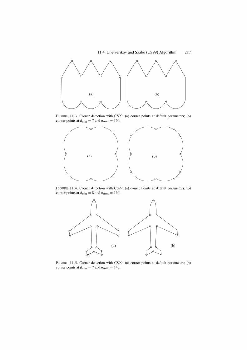
11.4. Chetverikov and Szabo (CS99) Algorithm 217
(a) (b)
FIGURE 11.3. Corner detection with CS99: (a) corner points at default parameters; (b)corner points at dmin = 7 and αmax = 160.
(a) (b)
FIGURE 11.4. Corner detection with CS99: (a) corner Points at default parameters; (b)corner points at dmin = 8 and αmax = 160.
(b)(a)
FIGURE 11.5. Corner detection with CS99: (a) corner points at default parameters; (b)corner points at dmin = 7 and αmax = 140.
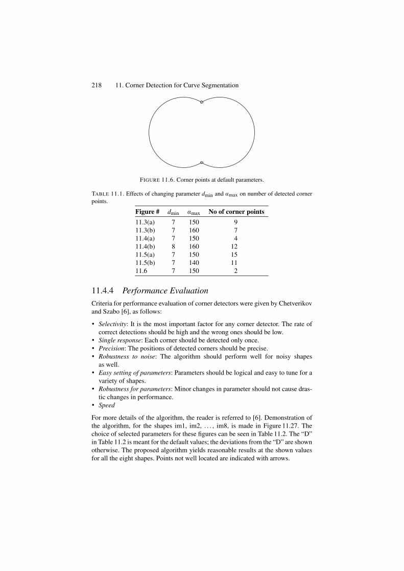
218 11. Corner Detection for Curve Segmentation
FIGURE 11.6. Corner points at default parameters.
TABLE 11.1. Effects of changing parameter dmin and αmax on number of detected cornerpoints.
Figure # dmin αmax No of corner points11.3(a) 7 150 911.3(b) 7 160 711.4(a) 7 150 411.4(b) 8 160 1211.5(a) 7 150 1511.5(b) 7 140 1111.6 7 150 2
11.4.4 Performance EvaluationCriteria for performance evaluation of corner detectors were given by Chetverikovand Szabo [6], as follows:
• Selectivity: It is the most important factor for any corner detector. The rate ofcorrect detections should be high and the wrong ones should be low.
• Single response: Each corner should be detected only once.• Precision: The positions of detected corners should be precise.• Robustness to noise: The algorithm should perform well for noisy shapes
as well.• Easy setting of parameters: Parameters should be logical and easy to tune for a
variety of shapes.• Robustness for parameters: Minor changes in parameter should not cause dras-
tic changes in performance.• Speed
For more details of the algorithm, the reader is referred to [6]. Demonstration ofthe algorithm, for the shapes im1, im2, . . . , im8, is made in Figure 11.27. Thechoice of selected parameters for these figures can be seen in Table 11.2. The “D”in Table 11.2 is meant for the default values; the deviations from the “D” are shownotherwise. The proposed algorithm yields reasonable results at the shown valuesfor all the eight shapes. Points not well located are indicated with arrows.
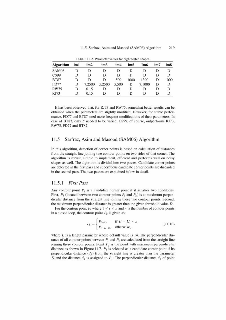
11.5. Sarfraz, Asim and Masood (SAM06) Algorithm 219
TABLE 11.2. Parameter values for eight tested shapes.
Algorithm im1 im2 im3 im4 im5 Im6 im7 im8SAM06 D D D D D D D DCS99 D D D D D D D DBT87 D D D 500 1000 1300 D 1000FD77 D 7,2500 5,2500 5,500 D 7,1000 D DRW75 D 0.15 D D D D D DRJ73 D 0.15 D D D D D D
It has been observed that, for RJ73 and RW75, somewhat better results can beobtained when the parameters are slightly modified. However, for stable perfor-mance, FD77 and BT87 need more frequent modifications of their parameters. Incase of BT87, only S needed to be varied. CS99, of course, outperforms RJ73,RW75, FD77 and BT87.
11.5 Sarfraz, Asim and Masood (SAM06) Algorithm
In this algorithm, detection of corner points is based on calculation of distancesfrom the straight line joining two contour points on two sides of that corner. Thealgorithm is robust, simple to implement, efficient and performs well on noisyshapes as well. The algorithm is divided into two passes. Candidate corner pointsare detected in the first pass and superfluous candidate corner points are discardedin the second pass. The two passes are explained below in detail.
11.5.1 First PassAny contour point Pj is a candidate corner point if it satisfies two conditions.First, Pj (located between two contour points Pi and Pk) is at maximum perpen-dicular distance from the straight line joining these two contour points. Second,the maximum perpendicular distance is greater than the given threshold value D.
For the contour point Pi where 1 ≤ i ≤ n and n is the number of contour pointsin a closed loop, the contour point Pk is given as:
Pk ={
Pi+L , if (i + L) ≤ n,
Pi+L−n, otherwise,(11.10)
where L is a length parameter whose default value is 14. The perpendicular dis-tance of all contour points between Pi and Pk are calculated from the straight linejoining these contour points. Point Pj is the point with maximum perpendiculardistance as shown in Figure 11.7. Pj is selected as a candidate corner point if itsperpendicular distance (d j ) from the straight line is greater than the parameterD and the distance d j is assigned to Pj . The perpendicular distance d j of point
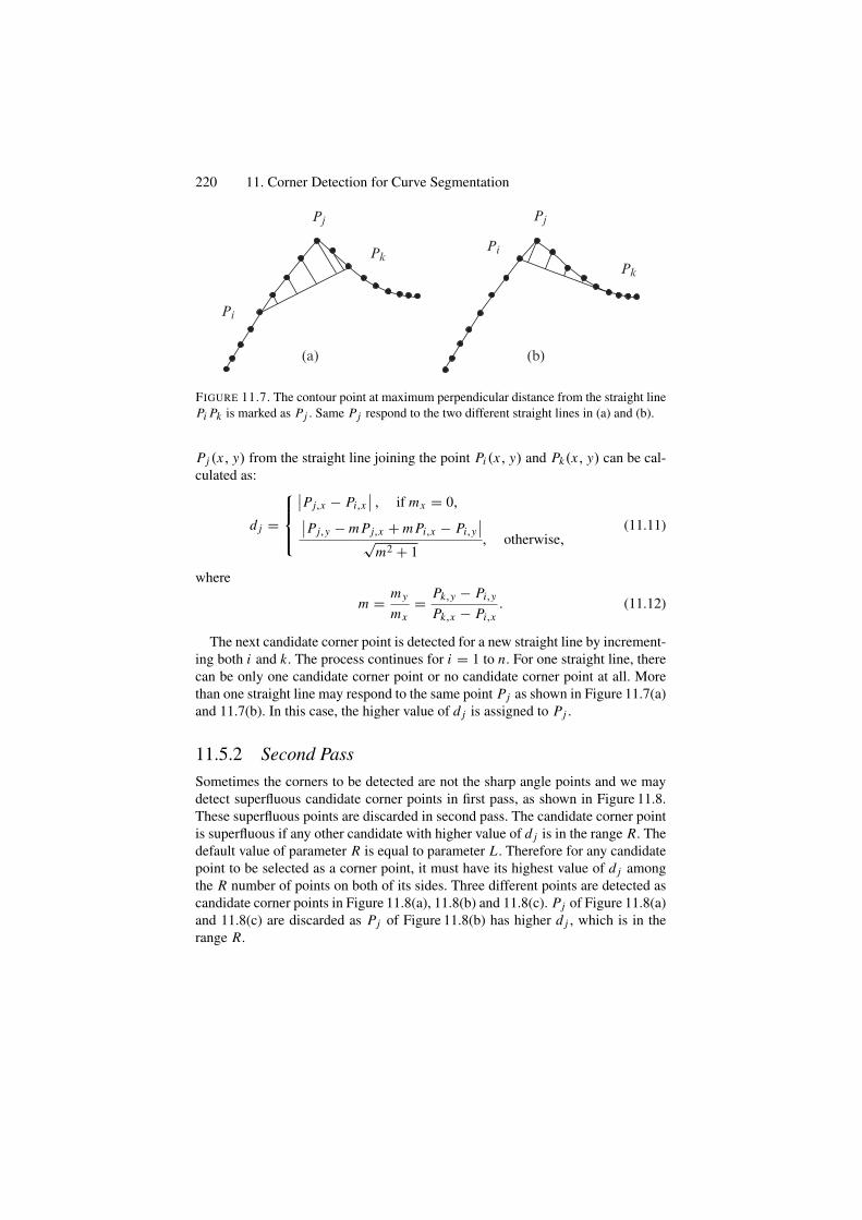
220 11. Corner Detection for Curve Segmentation
(a) (b)
Pi
Pi
PjPj
Pk
Pk
FIGURE 11.7. The contour point at maximum perpendicular distance from the straight linePi Pk is marked as Pj . Same Pj respond to the two different straight lines in (a) and (b).
Pj (x, y) from the straight line joining the point Pi (x, y) and Pk(x, y) can be cal-culated as:
d j =
⎧⎪⎨
⎪⎩
∣∣Pj,x − Pi,x∣∣ , if mx = 0,
∣∣Pj,y − m Pj,x + m Pi,x − Pi,y∣∣
√m2 + 1
, otherwise,(11.11)
where
m = my
mx= Pk,y − Pi,y
Pk,x − Pi,x. (11.12)
The next candidate corner point is detected for a new straight line by increment-ing both i and k. The process continues for i = 1 to n. For one straight line, therecan be only one candidate corner point or no candidate corner point at all. Morethan one straight line may respond to the same point Pj as shown in Figure 11.7(a)and 11.7(b). In this case, the higher value of d j is assigned to Pj .
11.5.2 Second PassSometimes the corners to be detected are not the sharp angle points and we maydetect superfluous candidate corner points in first pass, as shown in Figure 11.8.These superfluous points are discarded in second pass. The candidate corner pointis superfluous if any other candidate with higher value of d j is in the range R. Thedefault value of parameter R is equal to parameter L . Therefore for any candidatepoint to be selected as a corner point, it must have its highest value of d j amongthe R number of points on both of its sides. Three different points are detected ascandidate corner points in Figure 11.8(a), 11.8(b) and 11.8(c). Pj of Figure 11.8(a)and 11.8(c) are discarded as Pj of Figure 11.8(b) has higher d j , which is in therange R.
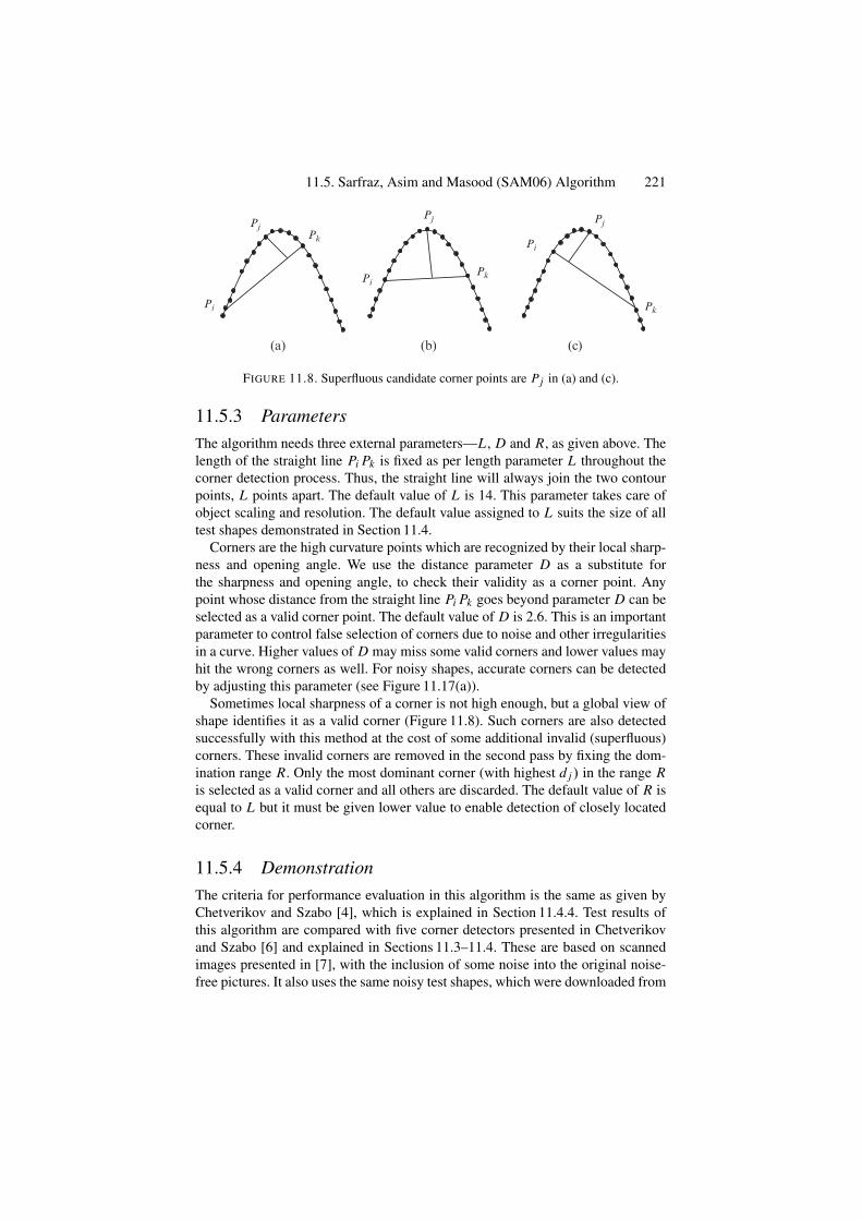
11.5. Sarfraz, Asim and Masood (SAM06) Algorithm 221
Pi
Pi
Pi
PjPj Pj
Pk
Pk
Pk
(c)(b)(a)
FIGURE 11.8. Superfluous candidate corner points are Pj in (a) and (c).
11.5.3 ParametersThe algorithm needs three external parameters—L , D and R, as given above. Thelength of the straight line Pi Pk is fixed as per length parameter L throughout thecorner detection process. Thus, the straight line will always join the two contourpoints, L points apart. The default value of L is 14. This parameter takes care ofobject scaling and resolution. The default value assigned to L suits the size of alltest shapes demonstrated in Section 11.4.
Corners are the high curvature points which are recognized by their local sharp-ness and opening angle. We use the distance parameter D as a substitute forthe sharpness and opening angle, to check their validity as a corner point. Anypoint whose distance from the straight line Pi Pk goes beyond parameter D can beselected as a valid corner point. The default value of D is 2.6. This is an importantparameter to control false selection of corners due to noise and other irregularitiesin a curve. Higher values of D may miss some valid corners and lower values mayhit the wrong corners as well. For noisy shapes, accurate corners can be detectedby adjusting this parameter (see Figure 11.17(a)).
Sometimes local sharpness of a corner is not high enough, but a global view ofshape identifies it as a valid corner (Figure 11.8). Such corners are also detectedsuccessfully with this method at the cost of some additional invalid (superfluous)corners. These invalid corners are removed in the second pass by fixing the dom-ination range R. Only the most dominant corner (with highest d j ) in the range Ris selected as a valid corner and all others are discarded. The default value of R isequal to L but it must be given lower value to enable detection of closely locatedcorner.
11.5.4 DemonstrationThe criteria for performance evaluation in this algorithm is the same as given byChetverikov and Szabo [4], which is explained in Section 11.4.4. Test results ofthis algorithm are compared with five corner detectors presented in Chetverikovand Szabo [6] and explained in Sections 11.3–11.4. These are based on scannedimages presented in [7], with the inclusion of some noise into the original noise-free pictures. It also uses the same noisy test shapes, which were downloaded from
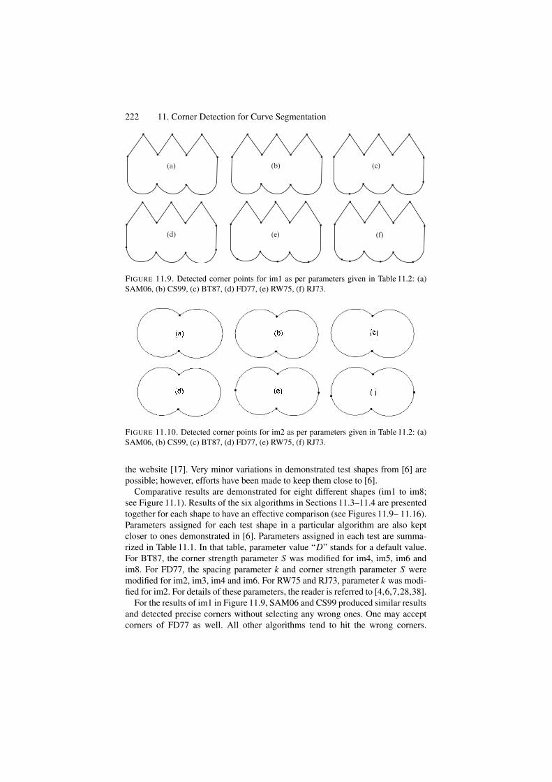
222 11. Corner Detection for Curve Segmentation
(c)
(f)(e)
(b)(a)
(d)
FIGURE 11.9. Detected corner points for im1 as per parameters given in Table 11.2: (a)SAM06, (b) CS99, (c) BT87, (d) FD77, (e) RW75, (f) RJ73.
FIGURE 11.10. Detected corner points for im2 as per parameters given in Table 11.2: (a)SAM06, (b) CS99, (c) BT87, (d) FD77, (e) RW75, (f) RJ73.
the website [17]. Very minor variations in demonstrated test shapes from [6] arepossible; however, efforts have been made to keep them close to [6].
Comparative results are demonstrated for eight different shapes (im1 to im8;see Figure 11.1). Results of the six algorithms in Sections 11.3–11.4 are presentedtogether for each shape to have an effective comparison (see Figures 11.9– 11.16).Parameters assigned for each test shape in a particular algorithm are also keptcloser to ones demonstrated in [6]. Parameters assigned in each test are summa-rized in Table 11.1. In that table, parameter value “D” stands for a default value.For BT87, the corner strength parameter S was modified for im4, im5, im6 andim8. For FD77, the spacing parameter k and corner strength parameter S weremodified for im2, im3, im4 and im6. For RW75 and RJ73, parameter k was modi-fied for im2. For details of these parameters, the reader is referred to [4,6,7,28,38].
For the results of im1 in Figure 11.9, SAM06 and CS99 produced similar resultsand detected precise corners without selecting any wrong ones. One may acceptcorners of FD77 as well. All other algorithms tend to hit the wrong corners.
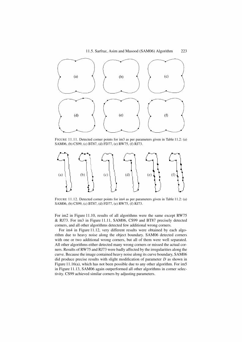
11.5. Sarfraz, Asim and Masood (SAM06) Algorithm 223
FIGURE 11.11. Detected corner points for im3 as per parameters given in Table 11.2: (a)SAM06, (b) CS99, (c) BT87, (d) FD77, (e) RW75, (f) RJ73.
(a) (b) (c) (d) (e) (f)
FIGURE 11.12. Detected corner points for im4 as per parameters given in Table 11.2: (a)SAM06, (b) CS99, (c) BT87, (d) FD77, (e) RW75, (f) RJ73.
For im2 in Figure 11.10, results of all algorithms were the same except RW75& RJ73. For im3 in Figure 11.11, SAM06, CS99 and BT87 precisely detectedcorners, and all other algorithms detected few additional wrong corners.
For im4 in Figure 11.12, very different results were obtained by each algo-rithm due to heavy noise along the object boundary. SAM06 detected cornerswith one or two additional wrong corners, but all of them were well separated.All other algorithms either detected many wrong corners or missed the actual cor-ners. Results of RW75 and RJ73 were badly affected by the irregularities along thecurve. Because the image contained heavy noise along its curve boundary, SAM06did produce precise results with slight modification of parameter D as shown inFigure 11.16(a), which has not been possible due to any other algorithm. For im5in Figure 11.13, SAM06 again outperformed all other algorithms in corner selec-tivity. CS99 achieved similar corners by adjusting parameters.
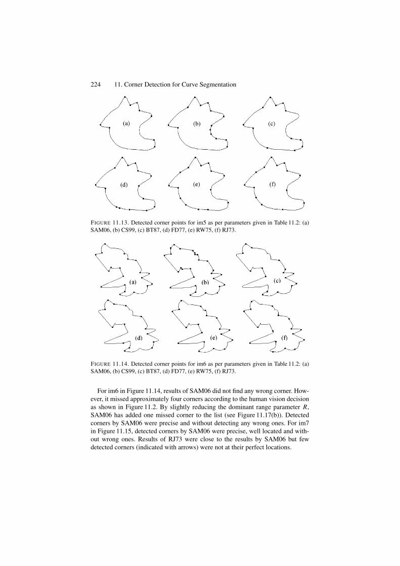
224 11. Corner Detection for Curve Segmentation
FIGURE 11.13. Detected corner points for im5 as per parameters given in Table 11.2: (a)SAM06, (b) CS99, (c) BT87, (d) FD77, (e) RW75, (f) RJ73.
FIGURE 11.14. Detected corner points for im6 as per parameters given in Table 11.2: (a)SAM06, (b) CS99, (c) BT87, (d) FD77, (e) RW75, (f) RJ73.
For im6 in Figure 11.14, results of SAM06 did not find any wrong corner. How-ever, it missed approximately four corners according to the human vision decisionas shown in Figure 11.2. By slightly reducing the dominant range parameter R,SAM06 has added one missed corner to the list (see Figure 11.17(b)). Detectedcorners by SAM06 were precise and without detecting any wrong ones. For im7in Figure 11.15, detected corners by SAM06 were precise, well located and with-out wrong ones. Results of RJ73 were close to the results by SAM06 but fewdetected corners (indicated with arrows) were not at their perfect locations.
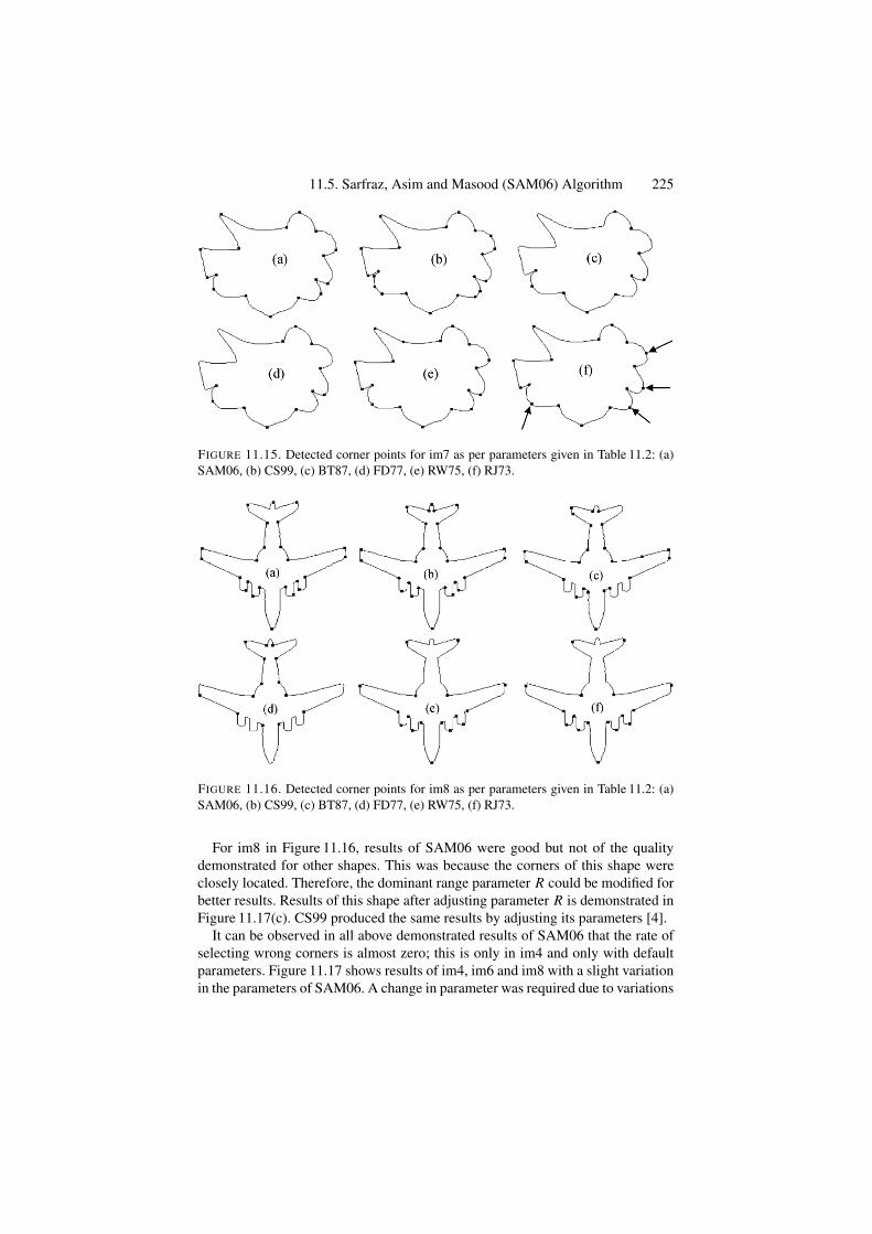
11.5. Sarfraz, Asim and Masood (SAM06) Algorithm 225
FIGURE 11.15. Detected corner points for im7 as per parameters given in Table 11.2: (a)SAM06, (b) CS99, (c) BT87, (d) FD77, (e) RW75, (f) RJ73.
FIGURE 11.16. Detected corner points for im8 as per parameters given in Table 11.2: (a)SAM06, (b) CS99, (c) BT87, (d) FD77, (e) RW75, (f) RJ73.
For im8 in Figure 11.16, results of SAM06 were good but not of the qualitydemonstrated for other shapes. This was because the corners of this shape wereclosely located. Therefore, the dominant range parameter R could be modified forbetter results. Results of this shape after adjusting parameter R is demonstrated inFigure 11.17(c). CS99 produced the same results by adjusting its parameters [4].
It can be observed in all above demonstrated results of SAM06 that the rate ofselecting wrong corners is almost zero; this is only in im4 and only with defaultparameters. Figure 11.17 shows results of im4, im6 and im8 with a slight variationin the parameters of SAM06. A change in parameter was required due to variations
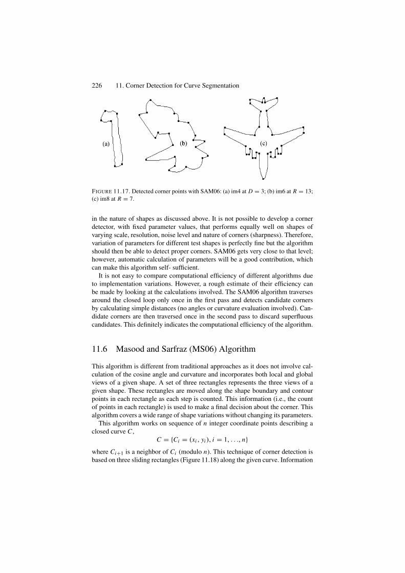
226 11. Corner Detection for Curve Segmentation
FIGURE 11.17. Detected corner points with SAM06: (a) im4 at D = 3; (b) im6 at R = 13;(c) im8 at R = 7.
in the nature of shapes as discussed above. It is not possible to develop a cornerdetector, with fixed parameter values, that performs equally well on shapes ofvarying scale, resolution, noise level and nature of corners (sharpness). Therefore,variation of parameters for different test shapes is perfectly fine but the algorithmshould then be able to detect proper corners. SAM06 gets very close to that level;however, automatic calculation of parameters will be a good contribution, whichcan make this algorithm self- sufficient.
It is not easy to compare computational efficiency of different algorithms dueto implementation variations. However, a rough estimate of their efficiency canbe made by looking at the calculations involved. The SAM06 algorithm traversesaround the closed loop only once in the first pass and detects candidate cornersby calculating simple distances (no angles or curvature evaluation involved). Can-didate corners are then traversed once in the second pass to discard superfluouscandidates. This definitely indicates the computational efficiency of the algorithm.
11.6 Masood and Sarfraz (MS06) Algorithm
This algorithm is different from traditional approaches as it does not involve cal-culation of the cosine angle and curvature and incorporates both local and globalviews of a given shape. A set of three rectangles represents the three views of agiven shape. These rectangles are moved along the shape boundary and contourpoints in each rectangle as each step is counted. This information (i.e., the countof points in each rectangle) is used to make a final decision about the corner. Thisalgorithm covers a wide range of shape variations without changing its parameters.
This algorithm works on sequence of n integer coordinate points describing aclosed curve C ,
C = {Ci = (xi , yi ), i = 1, . . ., n}where Ci+1 is a neighbor of Ci (modulo n). This technique of corner detection isbased on three sliding rectangles (Figure 11.18) along the given curve. Information
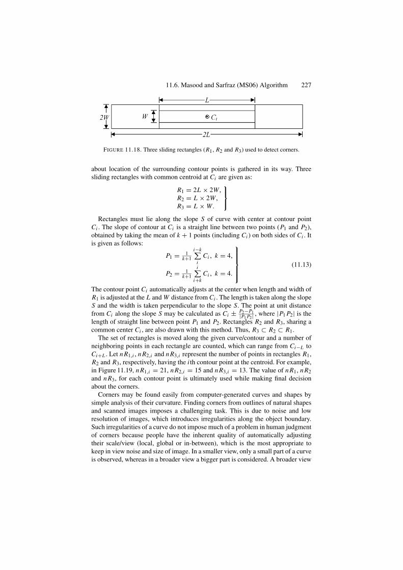
11.6. Masood and Sarfraz (MS06) Algorithm 227
FIGURE 11.18. Three sliding rectangles (R1, R2 and R3) used to detect corners.
about location of the surrounding contour points is gathered in its way. Threesliding rectangles with common centroid at Ci are given as:
R1 = 2L × 2W,R2 = L × 2W,R3 = L × W.
⎫⎬
⎭
Rectangles must lie along the slope S of curve with center at contour pointCi . The slope of contour at Ci is a straight line between two points (P1 and P2),obtained by taking the mean of k + 1 points (including Ci ) on both sides of Ci . Itis given as follows:
P1 = 1k+1
i−k∑
iCi , k = 4,
P2 = 1k+1
i∑
i+kCi , k = 4.
⎫⎪⎪⎪⎬
⎪⎪⎪⎭
(11.13)
The contour point Ci automatically adjusts at the center when length and width ofR1 is adjusted at the L and W distance from Ci . The length is taken along the slopeS and the width is taken perpendicular to the slope S. The point at unit distancefrom Ci along the slope S may be calculated as Ci ± P2−P1|P1 P2| , where |P1 P2| is thelength of straight line between point P1 and P2. Rectangles R2 and R3, sharing acommon center Ci , are also drawn with this method. Thus, R3 ⊂ R2 ⊂ R1.
The set of rectangles is moved along the given curve/contour and a number ofneighboring points in each rectangle are counted, which can range from Ci−L toCi+L . Let n R1,i , n R2,i and n R3,i represent the number of points in rectangles R1,R2 and R3, respectively, having the i th contour point at the centroid. For example,in Figure 11.19, n R1,i = 21, n R2,i = 15 and n R3,i = 13. The value of n R1, n R2and n R3, for each contour point is ultimately used while making final decisionabout the corners.
Corners may be found easily from computer-generated curves and shapes bysimple analysis of their curvature. Finding corners from outlines of natural shapesand scanned images imposes a challenging task. This is due to noise and lowresolution of images, which introduces irregularities along the object boundary.Such irregularities of a curve do not impose much of a problem in human judgmentof corners because people have the inherent quality of automatically adjustingtheir scale/view (local, global or in-between), which is the most appropriate tokeep in view noise and size of image. In a smaller view, only a small part of a curveis observed, whereas in a broader view a bigger part is considered. A broader view
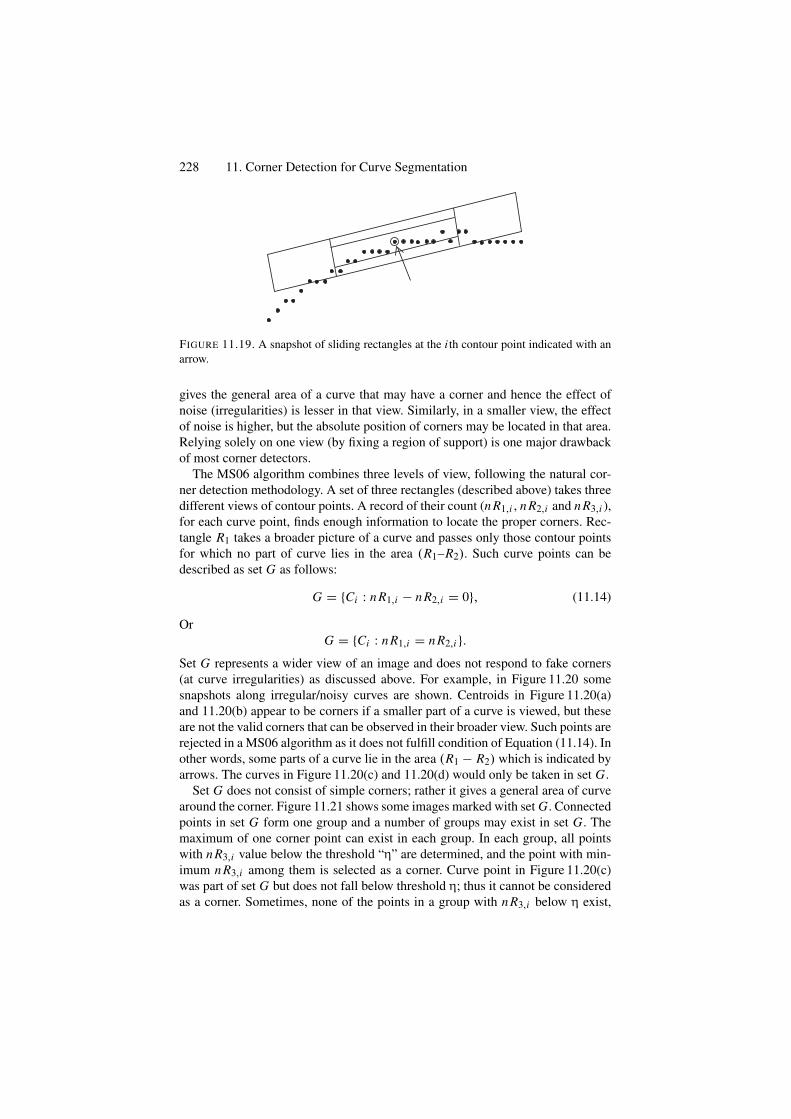
228 11. Corner Detection for Curve Segmentation
FIGURE 11.19. A snapshot of sliding rectangles at the i th contour point indicated with anarrow.
gives the general area of a curve that may have a corner and hence the effect ofnoise (irregularities) is lesser in that view. Similarly, in a smaller view, the effectof noise is higher, but the absolute position of corners may be located in that area.Relying solely on one view (by fixing a region of support) is one major drawbackof most corner detectors.
The MS06 algorithm combines three levels of view, following the natural cor-ner detection methodology. A set of three rectangles (described above) takes threedifferent views of contour points. A record of their count (n R1,i , n R2,i and n R3,i ),for each curve point, finds enough information to locate the proper corners. Rec-tangle R1 takes a broader picture of a curve and passes only those contour pointsfor which no part of curve lies in the area (R1–R2). Such curve points can bedescribed as set G as follows:
G = {Ci : n R1,i − n R2,i = 0}, (11.14)
OrG = {Ci : n R1,i = n R2,i }.
Set G represents a wider view of an image and does not respond to fake corners(at curve irregularities) as discussed above. For example, in Figure 11.20 somesnapshots along irregular/noisy curves are shown. Centroids in Figure 11.20(a)and 11.20(b) appear to be corners if a smaller part of a curve is viewed, but theseare not the valid corners that can be observed in their broader view. Such points arerejected in a MS06 algorithm as it does not fulfill condition of Equation (11.14). Inother words, some parts of a curve lie in the area (R1 − R2) which is indicated byarrows. The curves in Figure 11.20(c) and 11.20(d) would only be taken in set G.
Set G does not consist of simple corners; rather it gives a general area of curvearound the corner. Figure 11.21 shows some images marked with set G. Connectedpoints in set G form one group and a number of groups may exist in set G. Themaximum of one corner point can exist in each group. In each group, all pointswith n R3,i value below the threshold “η” are determined, and the point with min-imum n R3,i among them is selected as a corner. Curve point in Figure 11.20(c)was part of set G but does not fall below threshold η; thus it cannot be consideredas a corner. Sometimes, none of the points in a group with n R3,i below η exist,
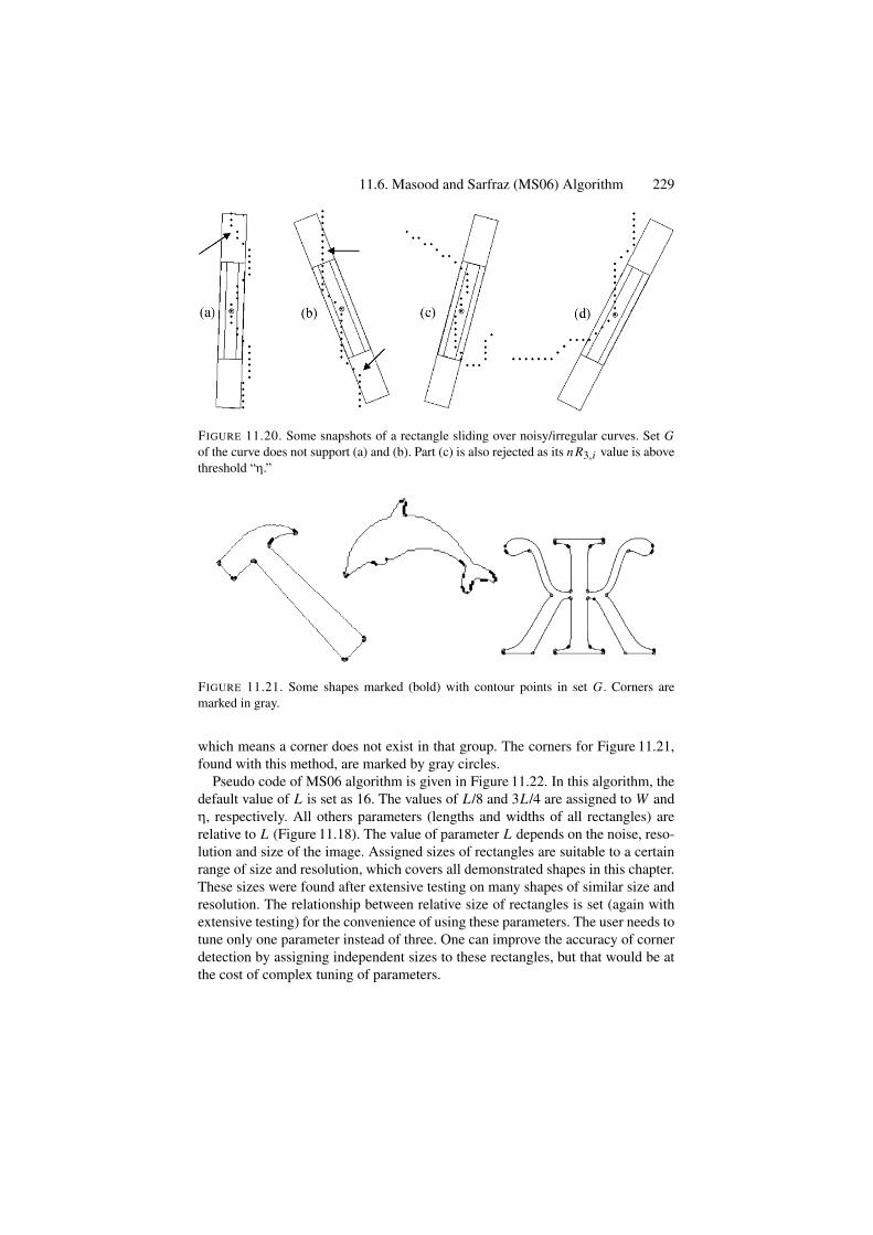
11.6. Masood and Sarfraz (MS06) Algorithm 229
FIGURE 11.20. Some snapshots of a rectangle sliding over noisy/irregular curves. Set Gof the curve does not support (a) and (b). Part (c) is also rejected as its n R3,i value is abovethreshold “η.”
FIGURE 11.21. Some shapes marked (bold) with contour points in set G. Corners aremarked in gray.
which means a corner does not exist in that group. The corners for Figure 11.21,found with this method, are marked by gray circles.
Pseudo code of MS06 algorithm is given in Figure 11.22. In this algorithm, thedefault value of L is set as 16. The values of L/8 and 3L/4 are assigned to W andη, respectively. All others parameters (lengths and widths of all rectangles) arerelative to L (Figure 11.18). The value of parameter L depends on the noise, reso-lution and size of the image. Assigned sizes of rectangles are suitable to a certainrange of size and resolution, which covers all demonstrated shapes in this chapter.These sizes were found after extensive testing on many shapes of similar size andresolution. The relationship between relative size of rectangles is set (again withextensive testing) for the convenience of using these parameters. The user needs totune only one parameter instead of three. One can improve the accuracy of cornerdetection by assigning independent sizes to these rectangles, but that would be atthe cost of complex tuning of parameters.
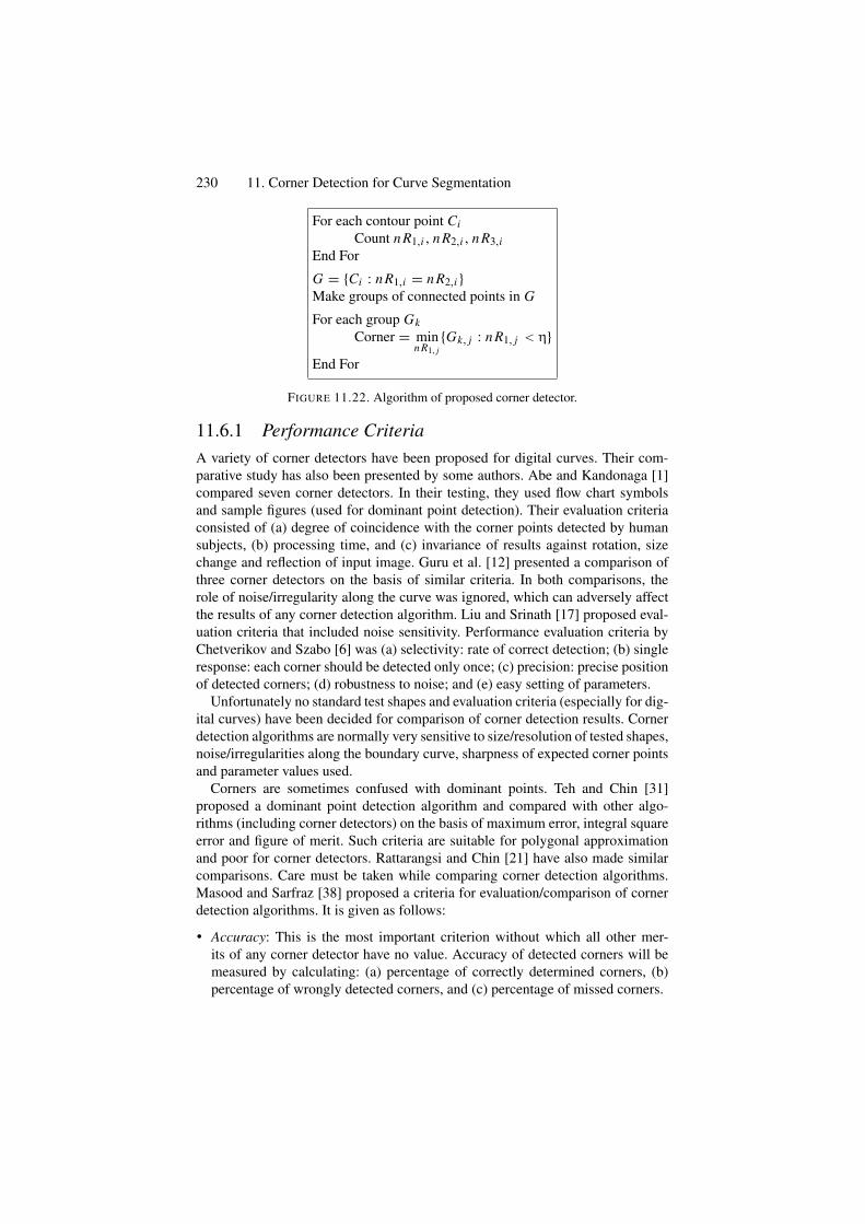
230 11. Corner Detection for Curve Segmentation
For each contour point CiCount n R1,i , n R2,i , n R3,i
End For
G = {Ci : n R1,i = n R2,i }Make groups of connected points in G
For each group GkCorner = min
n R1, j{Gk, j : n R1, j < η}
End For
FIGURE 11.22. Algorithm of proposed corner detector.
11.6.1 Performance CriteriaA variety of corner detectors have been proposed for digital curves. Their com-parative study has also been presented by some authors. Abe and Kandonaga [1]compared seven corner detectors. In their testing, they used flow chart symbolsand sample figures (used for dominant point detection). Their evaluation criteriaconsisted of (a) degree of coincidence with the corner points detected by humansubjects, (b) processing time, and (c) invariance of results against rotation, sizechange and reflection of input image. Guru et al. [12] presented a comparison ofthree corner detectors on the basis of similar criteria. In both comparisons, therole of noise/irregularity along the curve was ignored, which can adversely affectthe results of any corner detection algorithm. Liu and Srinath [17] proposed eval-uation criteria that included noise sensitivity. Performance evaluation criteria byChetverikov and Szabo [6] was (a) selectivity: rate of correct detection; (b) singleresponse: each corner should be detected only once; (c) precision: precise positionof detected corners; (d) robustness to noise; and (e) easy setting of parameters.
Unfortunately no standard test shapes and evaluation criteria (especially for dig-ital curves) have been decided for comparison of corner detection results. Cornerdetection algorithms are normally very sensitive to size/resolution of tested shapes,noise/irregularities along the boundary curve, sharpness of expected corner pointsand parameter values used.
Corners are sometimes confused with dominant points. Teh and Chin [31]proposed a dominant point detection algorithm and compared with other algo-rithms (including corner detectors) on the basis of maximum error, integral squareerror and figure of merit. Such criteria are suitable for polygonal approximationand poor for corner detectors. Rattarangsi and Chin [21] have also made similarcomparisons. Care must be taken while comparing corner detection algorithms.Masood and Sarfraz [38] proposed a criteria for evaluation/comparison of cornerdetection algorithms. It is given as follows:
• Accuracy: This is the most important criterion without which all other mer-its of any corner detector have no value. Accuracy of detected corners will bemeasured by calculating: (a) percentage of correctly determined corners, (b)percentage of wrongly detected corners, and (c) percentage of missed corners.
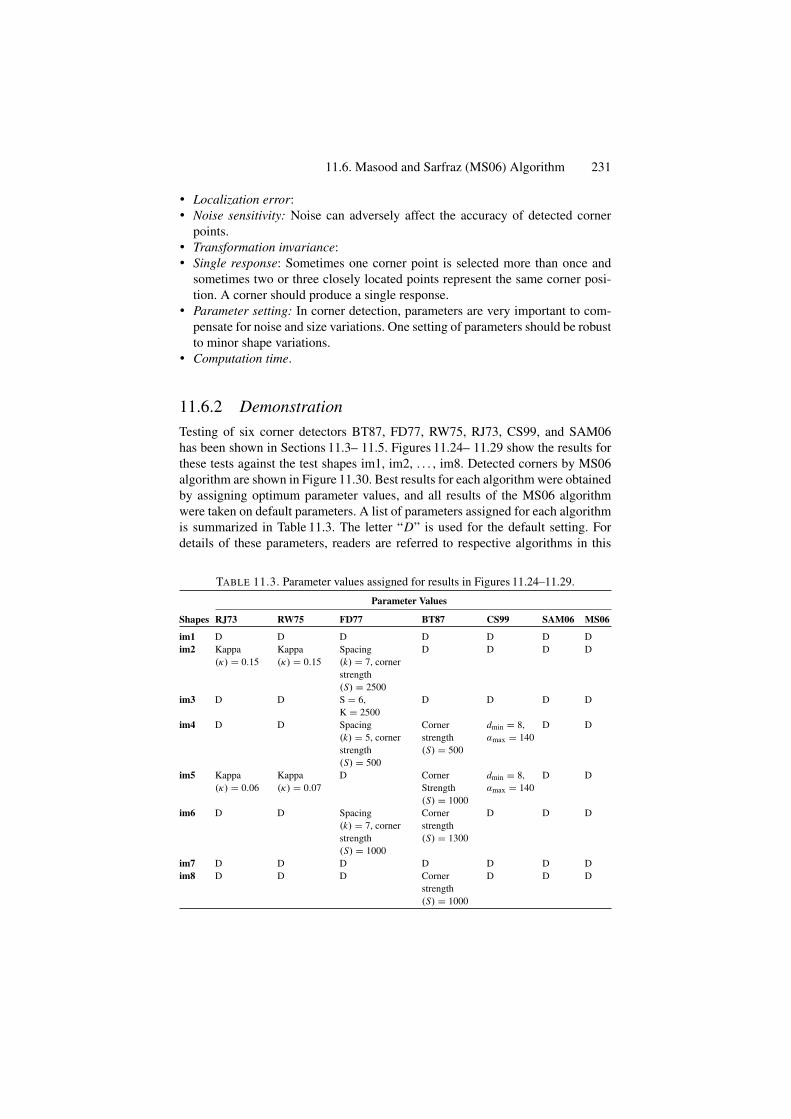
11.6. Masood and Sarfraz (MS06) Algorithm 231
• Localization error:• Noise sensitivity: Noise can adversely affect the accuracy of detected corner
points.• Transformation invariance:• Single response: Sometimes one corner point is selected more than once and
sometimes two or three closely located points represent the same corner posi-tion. A corner should produce a single response.
• Parameter setting: In corner detection, parameters are very important to com-pensate for noise and size variations. One setting of parameters should be robustto minor shape variations.
• Computation time.
11.6.2 DemonstrationTesting of six corner detectors BT87, FD77, RW75, RJ73, CS99, and SAM06has been shown in Sections 11.3– 11.5. Figures 11.24– 11.29 show the results forthese tests against the test shapes im1, im2, . . . , im8. Detected corners by MS06algorithm are shown in Figure 11.30. Best results for each algorithm were obtainedby assigning optimum parameter values, and all results of the MS06 algorithmwere taken on default parameters. A list of parameters assigned for each algorithmis summarized in Table 11.3. The letter “D” is used for the default setting. Fordetails of these parameters, readers are referred to respective algorithms in this
TABLE 11.3. Parameter values assigned for results in Figures 11.24–11.29.
Parameter Values
Shapes RJ73 RW75 FD77 BT87 CS99 SAM06 MS06
im1 D D D D D D Dim2 Kappa
(κ) = 0.15Kappa(κ) = 0.15
Spacing(k) = 7, cornerstrength(S) = 2500
D D D D
im3 D D S = 6,K = 2500
D D D D
im4 D D Spacing(k) = 5, cornerstrength(S) = 500
Cornerstrength(S) = 500
dmin = 8,αmax = 140
D D
im5 Kappa(κ) = 0.06
Kappa(κ) = 0.07
D CornerStrength(S) = 1000
dmin = 8,αmax = 140
D D
im6 D D Spacing(k) = 7, cornerstrength(S) = 1000
Cornerstrength(S) = 1300
D D D
im7 D D D D D D Dim8 D D D Corner
strength(S) = 1000
D D D
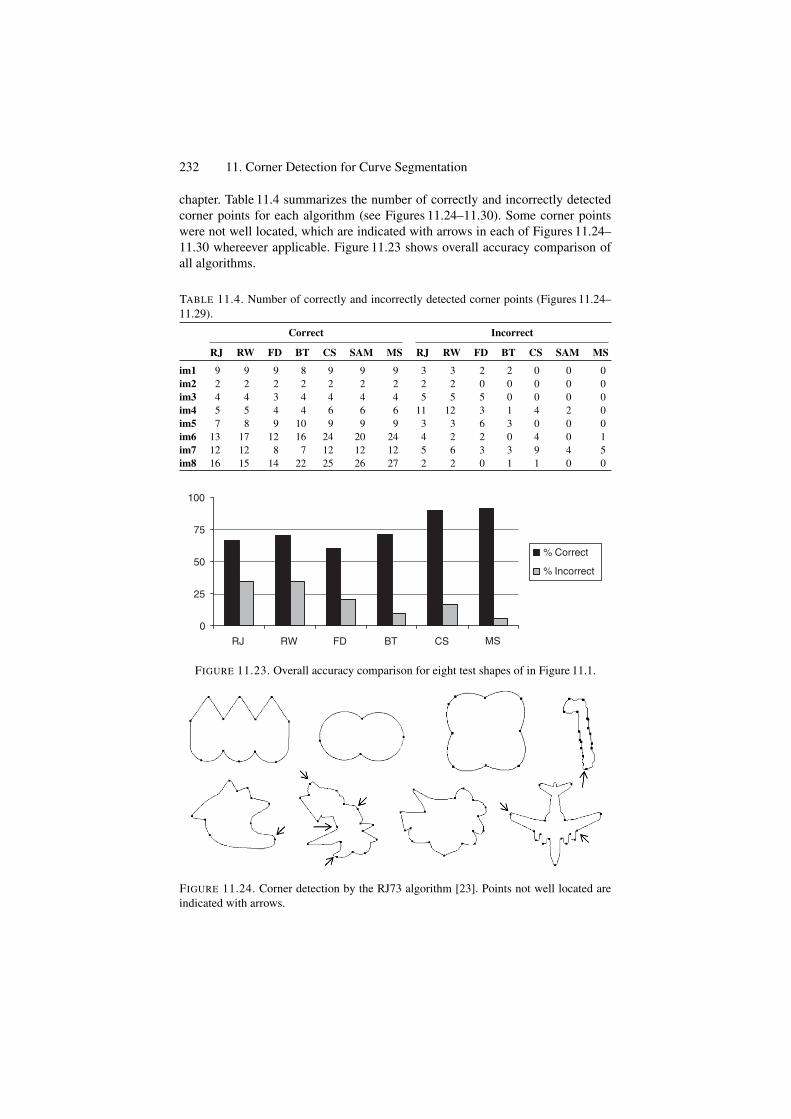
232 11. Corner Detection for Curve Segmentation
chapter. Table 11.4 summarizes the number of correctly and incorrectly detectedcorner points for each algorithm (see Figures 11.24–11.30). Some corner pointswere not well located, which are indicated with arrows in each of Figures 11.24–11.30 whereever applicable. Figure 11.23 shows overall accuracy comparison ofall algorithms.
TABLE 11.4. Number of correctly and incorrectly detected corner points (Figures 11.24–11.29).
Correct Incorrect
RJ RW FD BT CS SAM MS RJ RW FD BT CS SAM MS
im1 9 9 9 8 9 9 9 3 3 2 2 0 0 0im2 2 2 2 2 2 2 2 2 2 0 0 0 0 0im3 4 4 3 4 4 4 4 5 5 5 0 0 0 0im4 5 5 4 4 6 6 6 11 12 3 1 4 2 0im5 7 8 9 10 9 9 9 3 3 6 3 0 0 0im6 13 17 12 16 24 20 24 4 2 2 0 4 0 1im7 12 12 8 7 12 12 12 5 6 3 3 9 4 5im8 16 15 14 22 25 26 27 2 2 0 1 1 0 0
0
25
50
75
100
RJ RW FD BT CS
% Correct
% Incorrect
MS
FIGURE 11.23. Overall accuracy comparison for eight test shapes of in Figure 11.1.
FIGURE 11.24. Corner detection by the RJ73 algorithm [23]. Points not well located areindicated with arrows.
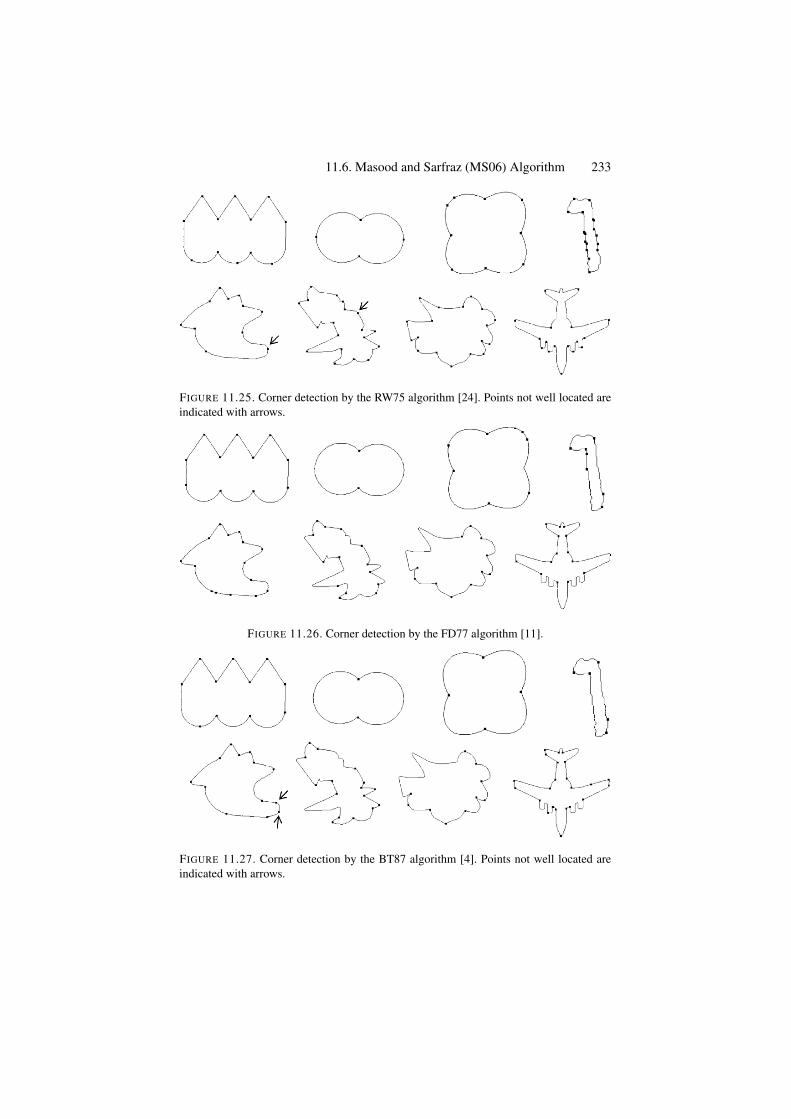
11.6. Masood and Sarfraz (MS06) Algorithm 233
FIGURE 11.25. Corner detection by the RW75 algorithm [24]. Points not well located areindicated with arrows.
FIGURE 11.26. Corner detection by the FD77 algorithm [11].
FIGURE 11.27. Corner detection by the BT87 algorithm [4]. Points not well located areindicated with arrows.
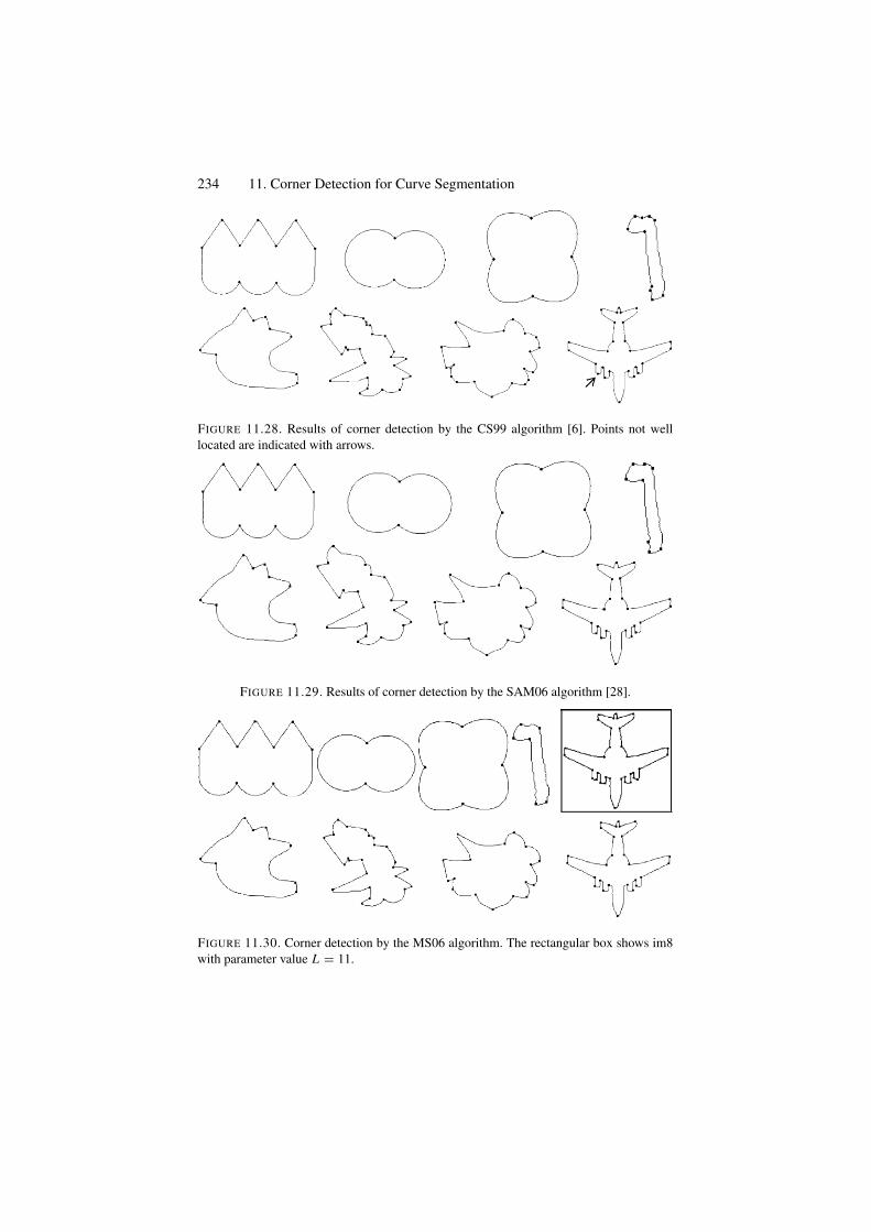
234 11. Corner Detection for Curve Segmentation
FIGURE 11.28. Results of corner detection by the CS99 algorithm [6]. Points not welllocated are indicated with arrows.
FIGURE 11.29. Results of corner detection by the SAM06 algorithm [28].
FIGURE 11.30. Corner detection by the MS06 algorithm. The rectangular box shows im8with parameter value L = 11.
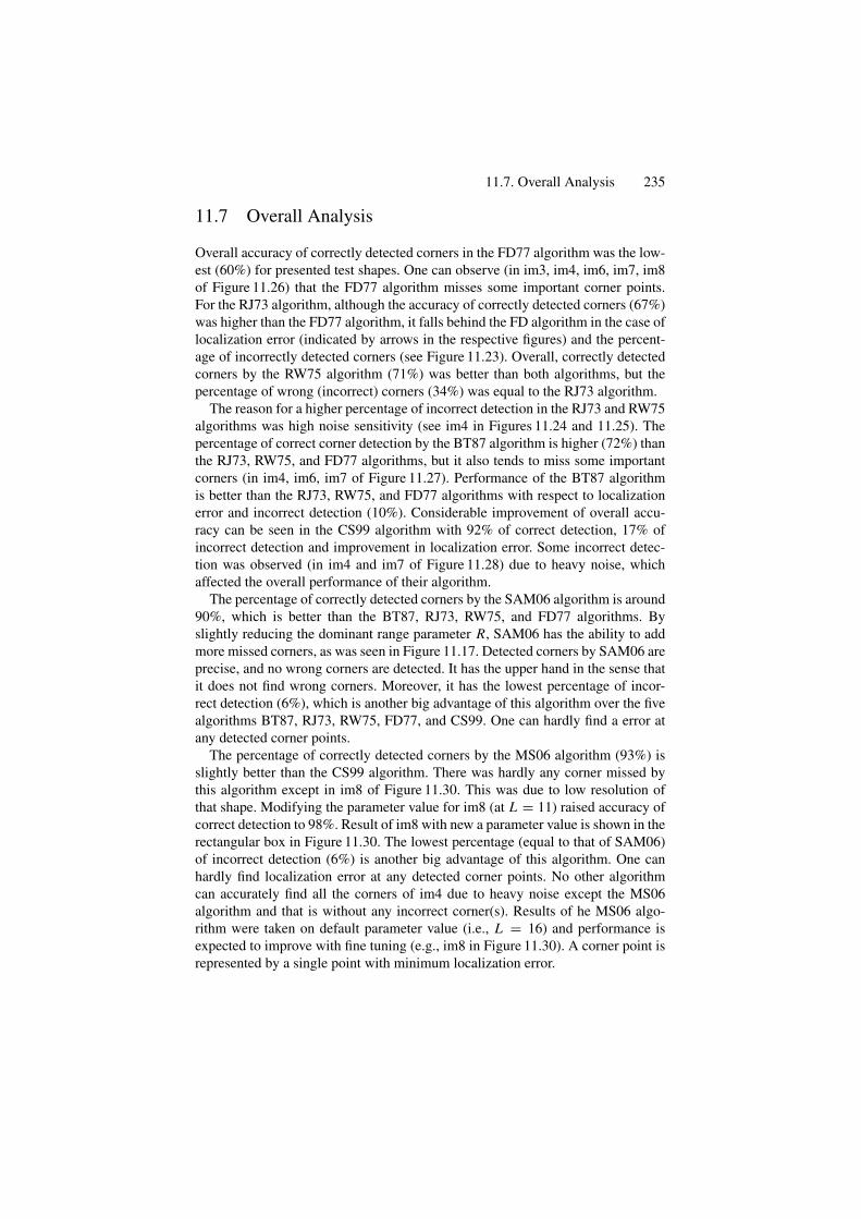
11.7. Overall Analysis 235
11.7 Overall Analysis
Overall accuracy of correctly detected corners in the FD77 algorithm was the low-est (60%) for presented test shapes. One can observe (in im3, im4, im6, im7, im8of Figure 11.26) that the FD77 algorithm misses some important corner points.For the RJ73 algorithm, although the accuracy of correctly detected corners (67%)was higher than the FD77 algorithm, it falls behind the FD algorithm in the case oflocalization error (indicated by arrows in the respective figures) and the percent-age of incorrectly detected corners (see Figure 11.23). Overall, correctly detectedcorners by the RW75 algorithm (71%) was better than both algorithms, but thepercentage of wrong (incorrect) corners (34%) was equal to the RJ73 algorithm.
The reason for a higher percentage of incorrect detection in the RJ73 and RW75algorithms was high noise sensitivity (see im4 in Figures 11.24 and 11.25). Thepercentage of correct corner detection by the BT87 algorithm is higher (72%) thanthe RJ73, RW75, and FD77 algorithms, but it also tends to miss some importantcorners (in im4, im6, im7 of Figure 11.27). Performance of the BT87 algorithmis better than the RJ73, RW75, and FD77 algorithms with respect to localizationerror and incorrect detection (10%). Considerable improvement of overall accu-racy can be seen in the CS99 algorithm with 92% of correct detection, 17% ofincorrect detection and improvement in localization error. Some incorrect detec-tion was observed (in im4 and im7 of Figure 11.28) due to heavy noise, whichaffected the overall performance of their algorithm.
The percentage of correctly detected corners by the SAM06 algorithm is around90%, which is better than the BT87, RJ73, RW75, and FD77 algorithms. Byslightly reducing the dominant range parameter R, SAM06 has the ability to addmore missed corners, as was seen in Figure 11.17. Detected corners by SAM06 areprecise, and no wrong corners are detected. It has the upper hand in the sense thatit does not find wrong corners. Moreover, it has the lowest percentage of incor-rect detection (6%), which is another big advantage of this algorithm over the fivealgorithms BT87, RJ73, RW75, FD77, and CS99. One can hardly find a error atany detected corner points.
The percentage of correctly detected corners by the MS06 algorithm (93%) isslightly better than the CS99 algorithm. There was hardly any corner missed bythis algorithm except in im8 of Figure 11.30. This was due to low resolution ofthat shape. Modifying the parameter value for im8 (at L = 11) raised accuracy ofcorrect detection to 98%. Result of im8 with new a parameter value is shown in therectangular box in Figure 11.30. The lowest percentage (equal to that of SAM06)of incorrect detection (6%) is another big advantage of this algorithm. One canhardly find localization error at any detected corner points. No other algorithmcan accurately find all the corners of im4 due to heavy noise except the MS06algorithm and that is without any incorrect corner(s). Results of he MS06 algo-rithm were taken on default parameter value (i.e., L = 16) and performance isexpected to improve with fine tuning (e.g., im8 in Figure 11.30). A corner point isrepresented by a single point with minimum localization error.
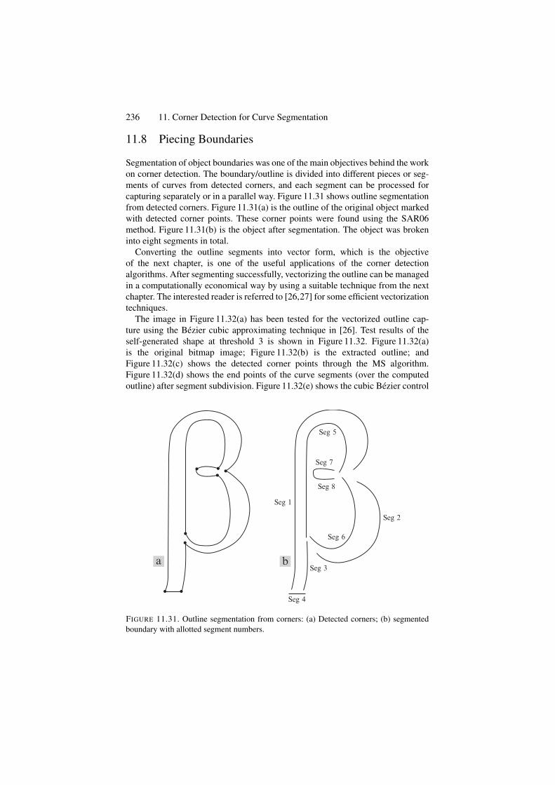
236 11. Corner Detection for Curve Segmentation
11.8 Piecing Boundaries
Segmentation of object boundaries was one of the main objectives behind the workon corner detection. The boundary/outline is divided into different pieces or seg-ments of curves from detected corners, and each segment can be processed forcapturing separately or in a parallel way. Figure 11.31 shows outline segmentationfrom detected corners. Figure 11.31(a) is the outline of the original object markedwith detected corner points. These corner points were found using the SAR06method. Figure 11.31(b) is the object after segmentation. The object was brokeninto eight segments in total.
Converting the outline segments into vector form, which is the objectiveof the next chapter, is one of the useful applications of the corner detectionalgorithms. After segmenting successfully, vectorizing the outline can be managedin a computationally economical way by using a suitable technique from the nextchapter. The interested reader is referred to [26,27] for some efficient vectorizationtechniques.
The image in Figure 11.32(a) has been tested for the vectorized outline cap-ture using the Bezier cubic approximating technique in [26]. Test results of theself-generated shape at threshold 3 is shown in Figure 11.32. Figure 11.32(a)is the original bitmap image; Figure 11.32(b) is the extracted outline; andFigure 11.32(c) shows the detected corner points through the MS algorithm.Figure 11.32(d) shows the end points of the curve segments (over the computedoutline) after segment subdivision. Figure 11.32(e) shows the cubic Bezier control
ba b
Seg 2
Seg 6
Seg 8
Seg 1
Seg 4
Seg 3
Seg 7
Seg 5
FIGURE 11.31. Outline segmentation from corners: (a) Detected corners; (b) segmentedboundary with allotted segment numbers.
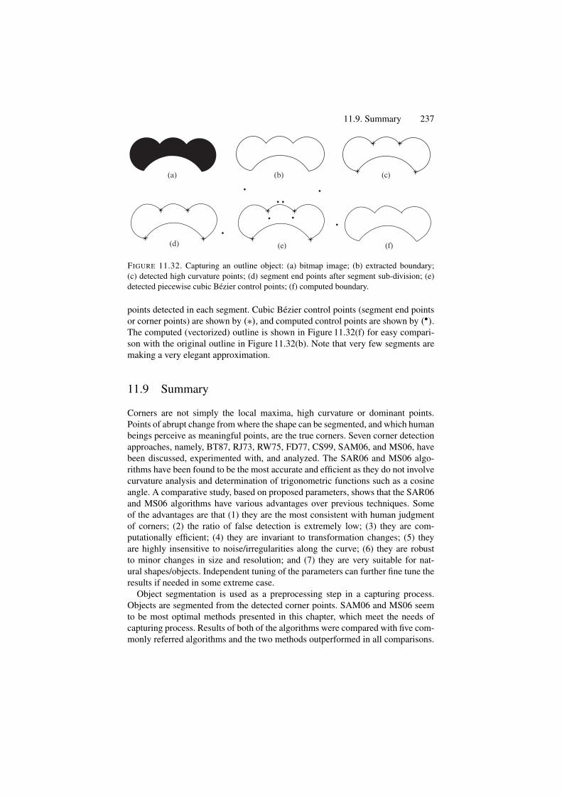
11.9. Summary 237
(a)
(d)
(b)
(e)
(c)
(f)
FIGURE 11.32. Capturing an outline object: (a) bitmap image; (b) extracted boundary;(c) detected high curvature points; (d) segment end points after segment sub-division; (e)detected piecewise cubic Bezier control points; (f) computed boundary.
points detected in each segment. Cubic Bezier control points (segment end pointsor corner points) are shown by (∗), and computed control points are shown by (•).The computed (vectorized) outline is shown in Figure 11.32(f) for easy compari-son with the original outline in Figure 11.32(b). Note that very few segments aremaking a very elegant approximation.
11.9 Summary
Corners are not simply the local maxima, high curvature or dominant points.Points of abrupt change from where the shape can be segmented, and which humanbeings perceive as meaningful points, are the true corners. Seven corner detectionapproaches, namely, BT87, RJ73, RW75, FD77, CS99, SAM06, and MS06, havebeen discussed, experimented with, and analyzed. The SAR06 and MS06 algo-rithms have been found to be the most accurate and efficient as they do not involvecurvature analysis and determination of trigonometric functions such as a cosineangle. A comparative study, based on proposed parameters, shows that the SAR06and MS06 algorithms have various advantages over previous techniques. Someof the advantages are that (1) they are the most consistent with human judgmentof corners; (2) the ratio of false detection is extremely low; (3) they are com-putationally efficient; (4) they are invariant to transformation changes; (5) theyare highly insensitive to noise/irregularities along the curve; (6) they are robustto minor changes in size and resolution; and (7) they are very suitable for nat-ural shapes/objects. Independent tuning of the parameters can further fine tune theresults if needed in some extreme case.
Object segmentation is used as a preprocessing step in a capturing process.Objects are segmented from the detected corner points. SAM06 and MS06 seemto be most optimal methods presented in this chapter, which meet the needs ofcapturing process. Results of both of the algorithms were compared with five com-monly referred algorithms and the two methods outperformed in all comparisons.
238 11. Corner Detection for Curve Segmentation
Specifically, MS06 was found to be slightly superior to Sam6. The algorithms areequally useful for any other application employing corner detection.
11.10 Exercises
1. Write a program to implement the following seven corner detectors—BT87,FD77, RW75, RJ73, CS99, SAM06, and MS06— described in Sections 11.3–11.6.
2. Test your programs for the test shapes im1, im2, . . . , im8 used in this chapter.3. Collect six different test images other than those used in this chapter and test
your programs for these test shapes.4. Using your program in Exercise 11.10.2, verify the results in Table 11.4 using
the parameter settings in Table 11.3.5. Using your program in Exercise 11.10.2, develop similar results as those in
Table 11.4 using the parameter settings in Table 11.3.6. Using your program in Exercise 11.10.2, develop similar results as those in
Table 11.4 using the parameter settings other than in Table 11.3.7. Develop a comparative study between your results obtained in Exercises
11.10.5 and 11.10.6.
References1. Abe, K., Morii, R., Nishida, K., and Kadonaga T. (1993), Comparison of methods for
detecting corner points from digital curves—a preliminary report, Int Conf DocumentAnal Recog 954–857.
2. Asada, H., and Brady, M. (1986). The curvature primal sketch, IEEE Trans PatternAnal Mach Intell PAMI-8, 2–4.
3. Attneave, F. (1954), Some informational aspects of visual perception, Psychol Rev61:183–193.
4. Beus, H.L., and Tiu, S.S.H. (1987), An improved corner detection algorithm based onchain coded plane curves, Pattern Rec 20:291–296.
5. Cabrelli, C.A., and Molter, U.M. (1990), Automatic representation of binary images,IEEE Trans Pattern Anal Mach Intell PAMI-12, 1190–1196.
6. Chetverikov, D., and Szabo, Z. (1999), A simple and efficient algorithm for detec-tion of high curvature points in planner curves, Proc. of 23rd Workshop of AustralianPattern Recognition Group, Steyr, pp.175–184.
7. Davies, E.R. (1988), Application of generalized Hough transform to corner detection,IEE-P(E:135), No. 1, pp. 49–54.
8. Deriche, R., and Giraudon, G. (1990), Accurate corner detection: an analytical study,Third International Conference on Computer Vision, pp. 66–70.
9. Deriche, R., and Faugeras, O.D. (1990), 2D curve matching using high curvaturepoints: application to stereo vision, 10th IAPR, pp. 18–23.
10. Dreschler, L., and Nagel, H.H. (1982), On the selection of critical points and localcurvature extrema of region boundaries for interframe matching, Proc. Of ICPR, pp.542–544.
References 239
11. Freeman, H., and Davis, L.S. (1977), A corner finding algorithm for chain-codedcurves, IEEE Trans Comput 26:297–303.
12. Guru, D.S., Dinesh, R., and Nagabhushan P. (2004), Boundary-based corner detectionand localization using new “cornerity” index: a robust approach, Proceedings of 1st
Canadian Conference on Computer and Robot Vision, pp. 417–423.13. Harris, C., and Stephens, M. (1988), A combined corner and edge detector, Proc Alvey
Vis Con, pp. 147–151.14. Kadonaga, T., and Abe, K. (1996), Comparison of methods for detecting corner points
from digital curves, GRMA95, pp 23–34.15. Kasturi, R., Siva, S., and O’Gorman, L. (1990), Techniques for line drawing inter-
pretation: an overview, Proc. IAPR Workshop on Machine Vision Applications, pp.151–160.
16. Kitchen, L., and Rosenfeld, A. (1982), Gray-level corner detection, Pattern Recog Lett1: 95–102.
17. Liu, H.C., and Srinath, L.S. (1990), Corner detection from chain- code, Pattern Recog23:51–68.
18. Mokhtarian, F., and Mackworth, A.K. (1992), A theory of multiscale, curvature-based shape representation for planar curves, IEEE Trans Pattern Anal Machine Intell14:789– 805.
19. Noble, J.A. (1988), Finding corners, Image Vision Comput 6:121–128, 1988.20. Pritchard, A.J., Sangwine, S.J., and Horne, R.E.N. (1993), Corner and curve detection
along a boundary using line segment triangles, Electronics Division Colloquium onHough Transforms, Digest No. 1993/106, pp. 1–4.
21. Rattarangsi, A., and Chin, R.T. (1992), Scale-based detection of corners of planarcurves, Trans Pattern Anal Machine Intell 14:430–449.
22. Ray, B.K., and Pandyan, R. (2003), ACORD: an adaptive corner detector for planarcurves, Pattern Recog 36:703–708.
23. Rosenfeld, A., and Johnston, E. (1973), Angle detection on digital curves, IEEE TransComput 22:875–878.
24. Rosenfeld, A., and Weszka, J.S. (1975), An improved method of angle detection ondigital curves, IEEE Trans Comput 24:940–941.
25. Rutkowski, W.S., and Rosenfeld, A. (1978), A comparison of corner-detection tech-niques for chain-coded curves, TR- 623, Computer Science Center, University ofMaryland.
26. Sarfraz, M., Asim, M.R., and Masood, A. (2004), Capturing outlines using cubic beziercurves, Proc. of IEEE 1st International Conference on Information & CommunicationTechnologies: from Theory to Applications, pp. 539–540.
27. Sarfraz, M., Masood, A., and Asim, M.R. (2004), A web-based system for capturingoutlines of 2D objects, Proceedings of International Conference on Information &Computer Science, Dhahran, Saudi Arabia.
28. Sarfraz, M., Asim, M.R., and Masood, A. (2006), A new approach to corner detec-tion:Computer Vision and Graphics, eds.: K. Wojciechowski, B. Smolka, H. Palus,R.S. Kozera, W. Skarbek, and L. Noakes, Springer-Verlag, New York, pp. 528–533.
29. Smith, P., Sinclair, D., Cipolla R., and Wood, K. (1998), Effective corner matching. In:P.H. Lewis and M.S. Nixon, eds., Proceedings of 9th British Machine Vision Confer-ence, volume II, pp. 545–556.
30. Smith, S., and Brady, J. (1995). SUSAN: a new approach to low- level imageprocessing, Int J Comput Vis 23, 45–78.

240 11. Corner Detection for Curve Segmentation
31. Teh C., and Chin, R. (1990), On the detection of dominant points on digital curves,IEEE Trans PAMI 8:859–873.
32. Vincent, E., and Laganiere, R. (2005), Detecting and matching feature points, J VisualCommun Image Representation 16(1), 38–54.
33. Vincent, E., and Laganire, R. (2001), Matching feature points in stereo pairs: a com-parative study of some matching strategies, Mach Graph Vis. 10:237–259.
34. Wang, H., and Brady, M. (1995), Real-time corner detection algorithm for motionestimation, Image Vision Comput, 13(9), 695–703.
35. Zoghlami, I., Faugeras, O., and Deriche, R. (1997), Using geometric corners to builda 2D mosaic from a set of images, Proc Comput Vis Pattern Recogn 420–425.
36. http://visual.ipan.sztaki.hu37. http://visual.ipan.sztaki.hu/publ/oagm99 corn.ps.gz38. Masood, A., and Sarfraz, M. (2006), A novel corner detector approach using slid-
ing rectangles, The Proceedings of the 4th ACS/IEEE International Conference onComputer Systems and Applications (AICCSA-06), Sharja, UAE, pp. 621–626, IEEEComputer Society Press.
12Linear Capture of Digital Curves
Abstract. This chapter is devoted to the detailed study of linear or polygonal approxi-mation needed in various applications, including shape recognition, point-based motionestimation, coding methods, and so on., in the areas of computer graphics, imaging andvision. Some important aspects related to capturing with linear approximation have beenaddressed. A detailed survey of many methods, in the current literature has been made.Some commonly referred algorithms have been explained and their results are demon-strated and compared.
12.1 Introduction
The most appealing representation of information to humans is in a visual form.Effective computer representation of these visual shapes is an important task.Boundary representation of shapes and their approximation economizes memorystorage and processing time for subsequent procedures.
The goal of a linear approximation is to capture the essence of boundary shapeswith the fewest possible segments. The term dominant point (DP) is assigned to theend points of these segments. Linear approximation for closed curves is referred toas polygonal approximation because approximating line segments joined togetherform a polygon. This is one of the popular approaches, which can provide goodrepresentations of 2D shapes at different resolutions. One obvious advantage ofusing this approach is high data reduction and its immediate impact on the effi-ciency of the subsequent feature extraction and/or shape-matching algorithms.It has been applied in shape recognition, point-based motion estimation, and cod-ing methods. This representation gained popularity due to its simplicity, locality,generality and compactness [22].
The development of this approach has its roots back to the research carriedout in psychology toward the study of shape perception and shape understanding.In one of his experiments, Attneave [1] created the picture of a cat by identifyinghigh curvature points in an ordinary snapshot, and linking them by line segments.A human observer easily recognized the resulting sketch. The conclusion was thatthose high curvature points are rich in information content, and they are able andsufficient to characterize a contour. These points are considered as representative
241
242 12. Linear Capture of Digital Curves
features for the object contours. This idea has been the starting point for mostof the subsequent efforts in this direction. Following Attneave’s [1] observation,there are many approaches developed for detection of dominant points.
Algorithms on polygonal/linear approximation can be classified into three maingroups, namely, sequential approach, split-and-merge approach and heuristic-search approach. For sequential approaches, Sklansky and Gonzales [23] pro-posed a scan-along procedure that starts from a point and tries to find the longestline segments sequentially. Ray and Ray [11] proposed a method that determinesthe longest possible line segments with the minimum possible error. Teh andChin [18] determined the region of support for each point based on its localproperties and computed its relative significance (curvature) and finally detecteddominant points by a process of nonmaxima suppression. Kurozumi and Davis [7]proposed a minimax method that derives the approximating segments by minimiz-ing the maximum distance between a given set of points and the correspondingsegments. Most of the sequential approaches are simple and fast, but the quality oftheir approximating results depends on the location of the point where they startthe scan-along process.
For split-and-merge approaches, Ramer [10] presented a recursive method start-ing with initial boundary segmentation. At each iteration, the segment was split atthe point that has the farthest distance from the corresponding segment unlessthe approximation error is no more than the prespecified error tolerance. Sarfrazet al. [14] proposed a recursive algorithm in which the longest line segments withinthe specified threshold were determined. Common points were marked as domi-nant points and curve segment was split into subsegments from each dominantpoint and processed recursively. Held et al, [24] proposed a split-and-merge tech-nique in which difference of slope was used to split segments and these weremerged on the criteria of perceptual significance. The approximation results ofthe split-and-merge approaches may be far from the optimal one if a poor initialsegmentation is used.
For the heuristic-search approach, an exhaustive search for the vertices of theoptimal polygon from the given set of data points will result in an exponentialcomplexity. Dunham [25] and Sato [26] used dynamic programming to find theoptimal approximating polygon. However, when the starting point is not specified,these methods require a worst-case complexity of O(n4) where n is the numberof data points. Some authors [27–30] have used a genetic algorithm for polygonalapproximation of digital curves. Tabu search [31] have been proposed to solve thepolygonal approximation problem and to obtain better results than most of thosedue to the local optimal methods. Yin [32] has proposed polygonal approxima-tion technique using ant colony search algorithm. Heuristic-search algorithms arecomputationally expensive and are not guaranteed to be optimal.
This chapter, in addition to the summary of various algorithms in the liter-ature, is dedicated for the recursive algorithm devised by Sarfraz et al. [14]for piecewise polygonal approximation of digital curves. For simplicity, the
12.2. Some Important Issues 243
algorithm will be called SAMAPA (Sarfraz-Asim-Masood Algorithm for Polygo-nal Approximation).
Algorithms developed for polygonal approximation and dominant point detec-tion can be classified into two categories. The first is to extract dominant points bycurvature evaluation [9,11,15,18–20] and second is by fitting the longest straight-line segments [5, 7, 10, 16, 17, 21]. Extraction of dominant points depends on theaccuracy of curvature evaluation and correct determination of the region of sup-port at each contour point. It is computationally more expensive and the resultsare far from optimal. Polygonal approximation of curves by fitting straight lines ismore logical and is an efficient approach. The SAMAPA technique explained inthis chapter belongs to the second category.
The break points, in this chapter, will be extracted as a preprocessing steptoward polygonal approximation. These break points are the candidates to beselected as the end points of approximating straight lines. While approximatingthe curve with straight lines, it is important to select the best end points of linessuch that the number of line segments and approximation error are minimized. Thepolygonal approximation will be carried out in clockwise as well as anticlockwisedirections around the given curve to look for an optimal solution between the two.
The organization of the chapter is as follows. Some important aspects related tocapturing with linear approximation have been addressed in the following section.The preprocessing stage is discussed in Section 12.2. The polygonal approxima-tion algorithm is discussed in Section 12.3. Experimental results are evaluated inSection 12.4. Finally, Section 12.5 concludes the chapter.
12.2 Some Important Issues
Research on polygonal approximation is based on the number of issues that havea direct impact on the quality and performance of these algorithms. These areselection of input parameters, finding region of support, error calculation, shapesto be used for testing, min-# and min-ε problems. A standard algorithm is expectedto address these issues and propose a solution. These issues are described belowin detail.
12.2.1 Input ParametersMost of the algorithms are based on one or more input parameters. These para-meters are selected based on the level of detail represented by the digital curve. Ingeneral, it is difficult to find a set of parameters suitable for a curve that consistsof multiple size features. This is a fundamental problem of scale because the fea-tures describing the shape of a curve vary enormously in size and extent, and thereis seldom a well-defined basis for choosing an appropriate scale (or smoothing)parameter that correspond to a particular feature size [33]. Some of the researchershave proposed algorithms that require no input parameters [18, 34–36].
244 12. Linear Capture of Digital Curves
12.2.2 Region of SupportThe determination of the region of support constitutes the major problem in var-ious dominant point detection algorithms. Although the exact term is attributedto Teh and Chin [18], a similar concept has been presented by Langridge [38],who pointed out that each boundary point of a closed curve should have its ownview of the curve. A dominant point should have a view that constitutes a mean-ingful region of support of the curve and should block the view from neighboringnondominant points. Rosenberg [39] noted that certain points of a convex blobperceptually dominate other points of the blob. He further presented methods forthe determination of regions of support with specific reference to convex blobs.
Teh and Chin [18] argued that the detection of dominant points relies primarilyon the precise determination of the region of support. To support their argument,they applied three different significance measures (k-curvature, 1-curvature andk-cosine) to different test shapes, and showed that once the region of support isdetermined properly, the choice of a particular significance measure does not pro-duce much difference. Marji and Siy [9] suggested that the choice of the signifi-cance measure is also an important factor that has to be chosen properly, even inthe presence of an accurate region-of-support measure. They proposed an algo-rithm for determination of correct region of support, which is sum of the lengthsof the left and right support arms. This issue is addressed in many other placesalso [9, 20, 40, 42].
12.2.3 Error MeasurementError measurement represents the deviation of an approximating polygon from theoriginal shape. Various types of errors are used for this purpose, depending on thetype of distortion under consideration. Let C = {pi = (xi , yi ), i = 1, . . ., n}}be the set of points describing a closed curve, where pi+1 is the neighbor of pi(modulo n). Let p j pk be a straight line of the approximating polygon. The basicerror for that straight line is calculated as a perpendicular distance of all pointsbetween p j and pk from that straight line. Variations of this error measurement inthe polygonal approximation are described as follows:
• Integral square error (ISE): It is used to assess the overall distortion caused bythe approximating polygon. It is defined as:
ISE =n∑
i=1
ei , (12.1)
where ei is the squared distance of i th curve point from the approximatingpolygon.
• Maximum error (MaxError): Maximum error is the maximum deviation of theapproximating polygon from the original curve. It is described as follows:
•MaxError = n
maxi=1
{ei }, (12.2)
where ei is error in i th point (squared distance).
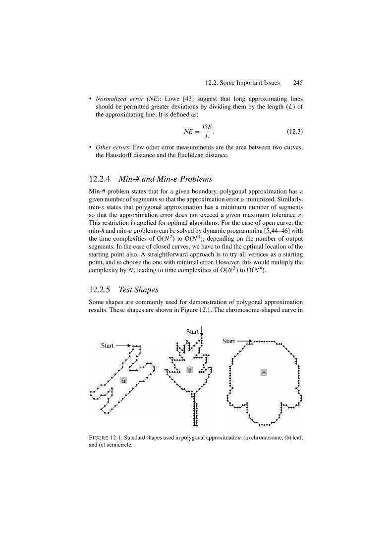
12.2. Some Important Issues 245
• Normalized error (NE): Lowe [43] suggest that long approximating linesshould be permitted greater deviations by dividing them by the length (L) ofthe approximating line. It is defined as:
NE = ISEL
. (12.3)
• Other errors: Few other error measurements are the area between two curves,the Hausdorff distance and the Euclidean distance.
12.2.4 Min-# and Min-ε ProblemsMin-# problem states that for a given boundary, polygonal approximation has agiven number of segments so that the approximation error is minimized. Similarly,min-ε states that polygonal approximation has a minimum number of segmentsso that the approximation error does not exceed a given maximum tolerance ε.This restriction is applied for optimal algorithms. For the case of open curve, themin-# and min-ε problems can be solved by dynamic programming [5,44–46] withthe time complexities of O(N 2) to O(N 3), depending on the number of outputsegments. In the case of closed curves, we have to find the optimal location of thestarting point also. A straightforward approach is to try all vertices as a startingpoint, and to choose the one with minimal error. However, this would multiply thecomplexity by N , leading to time complexities of O(N 3) to O(N 4).
12.2.5 Test ShapesSome shapes are commonly used for demonstration of polygonal approximationresults. These shapes are shown in Figure 12.1. The chromosome-shaped curve in
FIGURE 12.1. Standard shapes used in polygonal approximation: (a) chromosome, (b) leaf,and (c) semicircle.
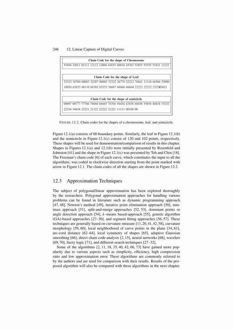
246 12. Linear Capture of Digital Curves
Chain Code for the shape of Chromosome
55454 32011 01111 12112 12006 65655 60010 10765 55455 55555 55431 12122
Chain Code for the shape of Leaf
33332 30700 00003 32307 00003 32322 26776 22212 76661 11116 66566 55000
10056 65655 00110 66565 65555 56667 66666 66664 22222 22222 23224 43433
Chain Code for the shape of semicircle
00007 00777 77766 76666 66665 76766 56454 43436 66656 55454 44434 33232
22254 54434 23221 21322 22222 21221 11111 00100 00
FIGURE 12.2. Chain codes for the shapes of a chromosome, leaf, and semicircle.
Figure 12.1(a) consists of 60 boundary points. Similarly, the leaf in Figure 12.1(b)and the semicircle in Figure 12.1(c) consist of 120 and 102 points, respectively.These shapes will be used for demonstration/comparison of results in this chapter.Shapes in Figures 12.1(a) and 12.1(b) were initially presented by Rosenfeld andJohnston [41] and the shape in Figure 12.1(c) was presented by Teh and Chin [18].The Freeman’s chain code [6] of each curve, which constitutes the input to all thealgorithms, was coded in clockwise direction starting from the point marked witharrow in Figure 12.1. The chain codes of all the shapes are shown in Figure 12.2.
12.3 Approximation Techniques
The subject of polygonal/linear approximation has been explored thoroughlyby the researchers. Polygonal approximation approaches for handling variousproblems can be found in literature such as dynamic programming approach[47, 48], Newton’s method [49], iterative point elimination approach [50], min-imax approach [51], split-and-merge approaches [52, 53], dominant points orangle detection approach [54], k–means based-approach [55], genetic algorithm(GA)-based approaches [27–30], and segment fitting approaches [56, 57]. Thesetechniques are generally based on curvature measure [11,20,41,42,58], curvaturemorphology [59, 60], local neighborhood of curve points in the plane [34, 61],arc-cord distance [62–64], local symmetry of shapes [65], adaptive Gaussiansmoothing [66], direct chain code analysis [2, 15], neural networks [68], wavelets[69, 70], fuzzy logic [71], and different search techniques [27–32].
Some of the algorithms [2, 11, 18, 35, 40, 42, 66, 73] have gained more pop-ularity due to various aspects such as simplicity, efficiency, high compressionratio and low approximation error. These algorithms are commonly referred toby the authors and are used for comparison with their results. Results of the pro-posed algorithm will also be compared with these algorithms in the next chapter.
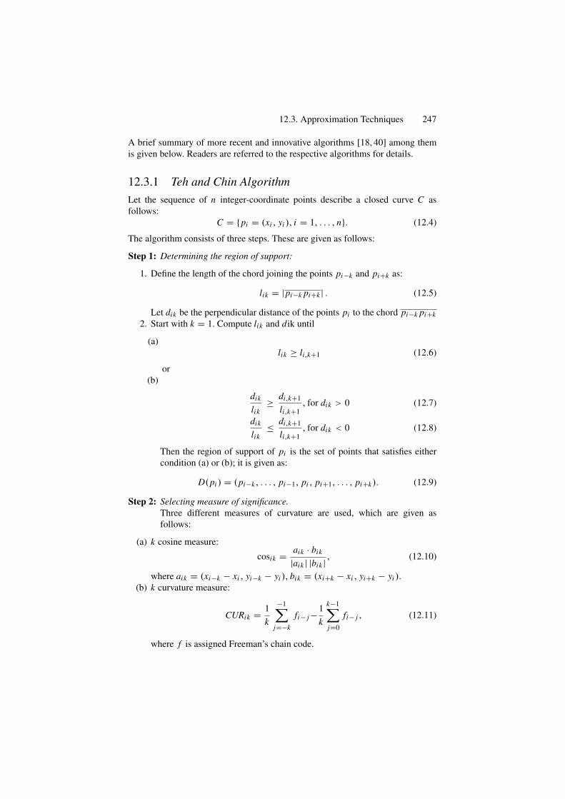
12.3. Approximation Techniques 247
A brief summary of more recent and innovative algorithms [18, 40] among themis given below. Readers are referred to the respective algorithms for details.
12.3.1 Teh and Chin AlgorithmLet the sequence of n integer-coordinate points describe a closed curve C asfollows:
C = {pi = (xi , yi ), i = 1, . . . , n}. (12.4)
The algorithm consists of three steps. These are given as follows:
Step 1: Determining the region of support:
1. Define the length of the chord joining the points pi−k and pi+k as:
lik = |pi−k pi+k | . (12.5)
Let dik be the perpendicular distance of the points pi to the chord pi−k pi+k2. Start with k = 1. Compute lik and dik until
(a)lik ≥ li,k+1 (12.6)
or(b)
dik
lik≥ di,k+1
li,k+1, for dik > 0 (12.7)
dik
lik≤ di,k+1
li,k+1, for dik < 0 (12.8)
Then the region of support of pi is the set of points that satisfies eithercondition (a) or (b); it is given as:
D(pi ) = (pi−k, . . . , pi−1, pi , pi+1, . . . , pi+k). (12.9)
Step 2: Selecting measure of significance.Three different measures of curvature are used, which are given asfollows:
(a) k cosine measure:
cosik = aik · bik
|aik | |bik | , (12.10)
where aik = (xi−k − xi , yi−k − yi ), bik = (xi+k − xi , yi+k − yi ).(b) k curvature measure:
CURik = 1k
−1∑
j=−k
fi− j−1k
k−1∑
j=0
fi− j , (12.11)
where f is assigned Freeman’s chain code.
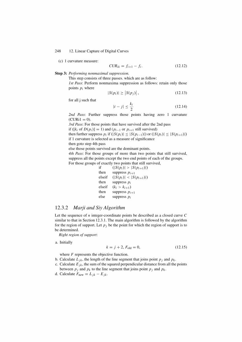
248 12. Linear Capture of Digital Curves
(c) 1 curvature measure:CURik = fi+1 − fi . (12.12)
Step 3: Performing nonmaximal suppression.This step consists of three passes. which are as follow:1st Pass: Perform nonmaxima suppression as follows: retain only thosepoints pi where
|S(pi )| ≥ ∣∣S(p j )∣∣ , (12.13)
for all j such that
|i − j | ≤ ki
2(12.14)
2nd Pass: Further suppress those points having zero 1 curvature(CURi1 = 0).3rd Pass: For those points that have survived after the 2nd passif ([ki of D(pi )] = 1) and (pi−1 or pi+1 still survived)then further suppress pi if (|S(pi )| ≤ |S(pi−1)|) or (|S(pi )| ≤ |S(pi+1)|)if 1 curvature is selected as a measure of significancethen goto step 4th passelse those points survived are the dominant points.4th Pass: For those groups of more than two points that still survived,suppress all the points except the two end points of each of the groups.For those groups of exactly two points that still survived,
if (|S(pi )| > |S(pi+1)|)then suppress pi+1elseif (|S(pi )| < |S(pi+1)|)then suppress pielseif (ki > ki+1)then suppress pi+1else suppress pi
12.3.2 Marji and Siy AlgorithmLet the sequence of n integer-coordinate points be described as a closed curve Csimilar to that in Section 12.3.1. The main algorithm is followed by the algorithmfor the region of support. Let p j be the point for which the region of support is tobe determined.
Right region of support:
a. Initiallyk = j + 2, Fold = 0, (12.15)
where F represents the objective function.b. Calculate L jk , the length of the line segment that joins point p j and pk .c. Calculate E jk , the sum of the squared perpendicular distance from all the points
between p j and pk to the line segment that joins point p j and pk .d. Calculate Fnew = L jk − E jk .
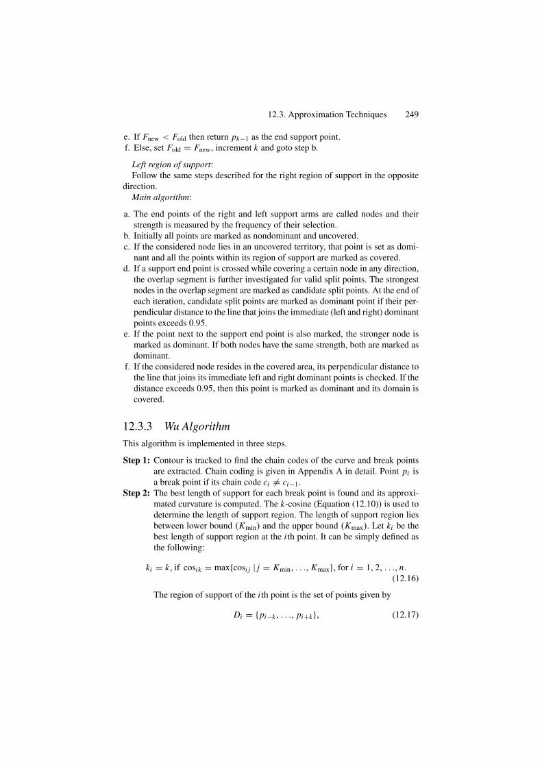
12.3. Approximation Techniques 249
e. If Fnew < Fold then return pk−1 as the end support point.f. Else, set Fold = Fnew, increment k and goto step b.
Left region of support:Follow the same steps described for the right region of support in the opposite
direction.Main algorithm:
a. The end points of the right and left support arms are called nodes and theirstrength is measured by the frequency of their selection.
b. Initially all points are marked as nondominant and uncovered.c. If the considered node lies in an uncovered territory, that point is set as domi-
nant and all the points within its region of support are marked as covered.d. If a support end point is crossed while covering a certain node in any direction,
the overlap segment is further investigated for valid split points. The strongestnodes in the overlap segment are marked as candidate split points. At the end ofeach iteration, candidate split points are marked as dominant point if their per-pendicular distance to the line that joins the immediate (left and right) dominantpoints exceeds 0.95.
e. If the point next to the support end point is also marked, the stronger node ismarked as dominant. If both nodes have the same strength, both are marked asdominant.
f. If the considered node resides in the covered area, its perpendicular distance tothe line that joins its immediate left and right dominant points is checked. If thedistance exceeds 0.95, then this point is marked as dominant and its domain iscovered.
12.3.3 Wu AlgorithmThis algorithm is implemented in three steps.
Step 1: Contour is tracked to find the chain codes of the curve and break pointsare extracted. Chain coding is given in Appendix A in detail. Point pi isa break point if its chain code ci = ci−1.
Step 2: The best length of support for each break point is found and its approxi-mated curvature is computed. The k-cosine (Equation (12.10)) is used todetermine the length of support region. The length of support region liesbetween lower bound (Kmin) and the upper bound (Kmax). Let ki be thebest length of support region at the i th point. It can be simply defined asthe following:
ki = k, if cosik = max{cosi j | j = Kmin, . . ., Kmax}, for i = 1, 2, . . ., n.(12.16)
The region of support of the i th point is the set of points given by
Di = {pi−k, . . ., pi+k}, (12.17)
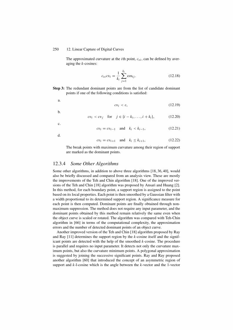
250 12. Linear Capture of Digital Curves
The approximated curvature at the i th point, cvi , can be defined by aver-aging the k-cosines:
cvi cvi = 1ki
ki∑
j=1
cosi j . (12.18)
Step 3: The redundant dominant points are from the list of candidate dominantpoints if one of the following conditions is satisfied:
a.cvi < ε, (12.19)
b.cvi < cv j for j ∈ {i − ki , . . . , i + ki }, (12.20)
c.cvi = cvi−1 and ki < ki−1, (12.21)
d.cvi = cvi+1 and ki ≤ ki+1, (12.22)
The break points with maximum curvature among their region of supportare marked as the dominant points.
12.3.4 Some Other AlgorithmsSome other algorithms, in addition to above three algorithms [18, 36, 40], wouldalso be briefly discussed and compared from an analysis view. These are mostlythe improvements of the Teh and Chin algorithm [18]. One of the improved ver-sions of the Teh and Chin [18] algorithm was proposed by Ansari and Huang [2].In this method, for each boundary point, a support region is assigned to the pointbased on its local properties. Each point is then smoothed by a Gaussian filter witha width proportional to its determined support region. A significance measure foreach point is then computed. Dominant points are finally obtained through non-maximum suppression. The method does not require any input parameter, and thedominant points obtained by this method remain relatively the same even whenthe object curve is scaled or rotated. The algorithm was compared with Teh-Chinalgorithm in [66] in terms of the computational complexity, the approximationerrors and the number of detected dominant points of an object curve.
Another improved version of the Teh and Chin [18] algorithm proposed by Rayand Ray [11] determines the support region by the k-cosine itself and the signif-icant points are detected with the help of the smoothed k-cosine. The procedureis parallel and requires no input parameter. It detects not only the curvature max-imum points, but also the curvature minimum points. A polygonal approximationis suggested by joining the successive significant points. Ray and Ray proposedanother algorithm [60] that introduced the concept of an asymmetric region ofsupport and k-l-cosine which is the angle between the k-vector and the 1-vector
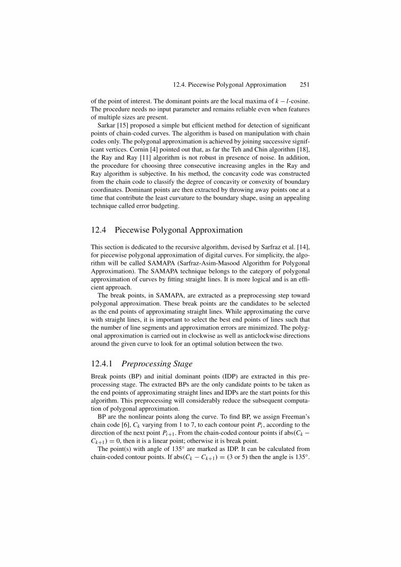
12.4. Piecewise Polygonal Approximation 251
of the point of interest. The dominant points are the local maxima of k − l-cosine.The procedure needs no input parameter and remains reliable even when featuresof multiple sizes are present.
Sarkar [15] proposed a simple but efficient method for detection of significantpoints of chain-coded curves. The algorithm is based on manipulation with chaincodes only. The polygonal approximation is achieved by joining successive signif-icant vertices. Cornin [4] pointed out that, as far the Teh and Chin algorithm [18],the Ray and Ray [11] algorithm is not robust in presence of noise. In addition,the procedure for choosing three consecutive increasing angles in the Ray andRay algorithm is subjective. In his method, the concavity code was constructedfrom the chain code to classify the degree of concavity or convexity of boundarycoordinates. Dominant points are then extracted by throwing away points one at atime that contribute the least curvature to the boundary shape, using an appealingtechnique called error budgeting.
12.4 Piecewise Polygonal Approximation
This section is dedicated to the recursive algorithm, devised by Sarfraz et al. [14],for piecewise polygonal approximation of digital curves. For simplicity, the algo-rithm will be called SAMAPA (Sarfraz-Asim-Masood Algorithm for PolygonalApproximation). The SAMAPA technique belongs to the category of polygonalapproximation of curves by fitting straight lines. It is more logical and is an effi-cient approach.
The break points, in SAMAPA, are extracted as a preprocessing step towardpolygonal approximation. These break points are the candidates to be selectedas the end points of approximating straight lines. While approximating the curvewith straight lines, it is important to select the best end points of lines such thatthe number of line segments and approximation errors are minimized. The polyg-onal approximation is carried out in clockwise as well as anticlockwise directionsaround the given curve to look for an optimal solution between the two.
12.4.1 Preprocessing StageBreak points (BP) and initial dominant points (IDP) are extracted in this pre-processing stage. The extracted BPs are the only candidate points to be taken asthe end points of approximating straight lines and IDPs are the start points for thisalgorithm. This preprocessing will considerably reduce the subsequent computa-tion of polygonal approximation.
BP are the nonlinear points along the curve. To find BP, we assign Freeman’schain code [6], Ck varying from 1 to 7, to each contour point Pi , according to thedirection of the next point Pi+1. From the chain-coded contour points if abs(Ck −Ck+1) = 0, then it is a linear point; otherwise it is break point.
The point(s) with angle of 135◦ are marked as IDP. It can be calculated fromchain-coded contour points. If abs(Ck − Ck+1) = (3 or 5) then the angle is 135◦.
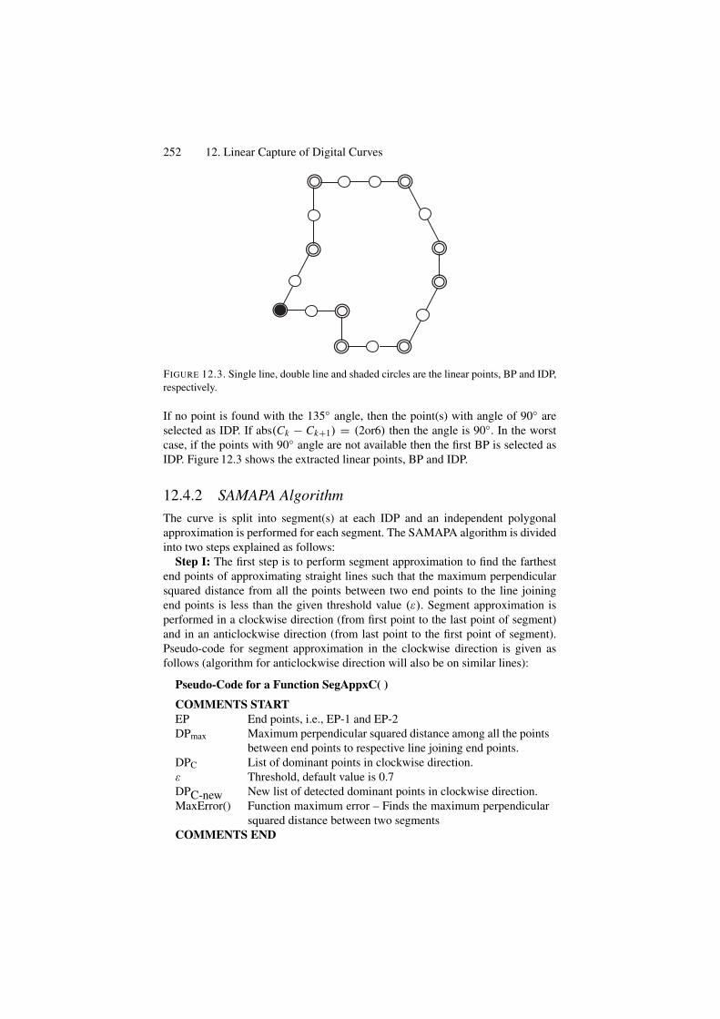
252 12. Linear Capture of Digital Curves
FIGURE 12.3. Single line, double line and shaded circles are the linear points, BP and IDP,respectively.
If no point is found with the 135◦ angle, then the point(s) with angle of 90◦ areselected as IDP. If abs(Ck − Ck+1) = (2or6) then the angle is 90◦. In the worstcase, if the points with 90◦ angle are not available then the first BP is selected asIDP. Figure 12.3 shows the extracted linear points, BP and IDP.
12.4.2 SAMAPA AlgorithmThe curve is split into segment(s) at each IDP and an independent polygonalapproximation is performed for each segment. The SAMAPA algorithm is dividedinto two steps explained as follows:
Step I: The first step is to perform segment approximation to find the farthestend points of approximating straight lines such that the maximum perpendicularsquared distance from all the points between two end points to the line joiningend points is less than the given threshold value (ε). Segment approximation isperformed in a clockwise direction (from first point to the last point of segment)and in an anticlockwise direction (from last point to the first point of segment).Pseudo-code for segment approximation in the clockwise direction is given asfollows (algorithm for anticlockwise direction will also be on similar lines):
Pseudo-Code for a Function SegAppxC( )
COMMENTS STARTEP End points, i.e., EP-1 and EP-2DPmax Maximum perpendicular squared distance among all the points
between end points to respective line joining end points.DPC List of dominant points in clockwise direction.ε Threshold, default value is 0.7DPC-new New list of detected dominant points in clockwise direction.MaxError() Function maximum error – Finds the maximum perpendicular
squared distance between two segmentsCOMMENTS END

12.4. Piecewise Polygonal Approximation 253
Function DPC = SegAppxC(Segment)DPC = [ ]DoEP-1 = first point of segmentEP-2 = next BP in sequenceDPC−new = [ ]DoDoCalculate DmaxIf Dmax < ε
P = EP-2End If
EP2 = next BPWhile ((Dmax < 2∗ε) OR (End of Segment))
EP-1 = PAdd P in the list DPC-newWhile (End of Segment)If isempty (DPC)DPC = DPC−newEnd Ifε = MaxError ( )While Length (DPnew) == Length(DPC)
Step II: The second step is to find an optimum solution between the two seg-ment approximations. The pseudo-code for the complete SAMAPA algorithm, asa recursive function “SAMAPA()”, is given as follows:
Pseudo-Code for the Function SAMAPA( )
Function DP = SAMAPA(Segment)DP = [ ]DPC = SegAppxC(Segment)DPA = SegAppxA(Segment)
If DPC ∪ DPA = φDP = segment end pointsReturn DP
End IfIf DPC ∩ DPA = φDivide segment into subsegments at (DPC ∩ DPA)For (each subsegment)DP = DP + SAMAPA(subsegment)End ForReturn DP
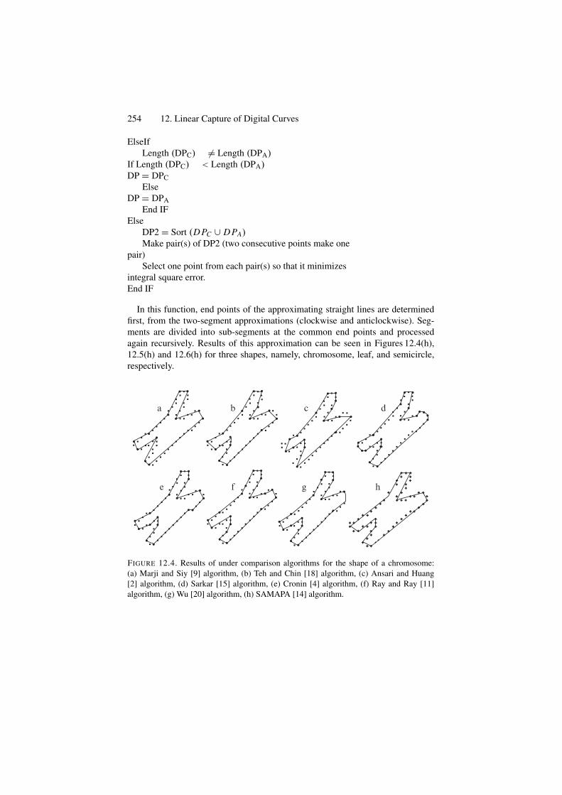
254 12. Linear Capture of Digital Curves
ElseIfLength (DPC) = Length (DPA)
If Length (DPC) < Length (DPA)DP = DPC
ElseDP = DPA
End IFElse
DP2 = Sort (D PC ∪ D PA)Make pair(s) of DP2 (two consecutive points make one
pair)Select one point from each pair(s) so that it minimizes
integral square error.End IF
In this function, end points of the approximating straight lines are determinedfirst, from the two-segment approximations (clockwise and anticlockwise). Seg-ments are divided into sub-segments at the common end points and processedagain recursively. Results of this approximation can be seen in Figures 12.4(h),12.5(h) and 12.6(h) for three shapes, namely, chromosome, leaf, and semicircle,respectively.
dba
e f g h
c
FIGURE 12.4. Results of under comparison algorithms for the shape of a chromosome:(a) Marji and Siy [9] algorithm, (b) Teh and Chin [18] algorithm, (c) Ansari and Huang[2] algorithm, (d) Sarkar [15] algorithm, (e) Cronin [4] algorithm, (f) Ray and Ray [11]algorithm, (g) Wu [20] algorithm, (h) SAMAPA [14] algorithm.
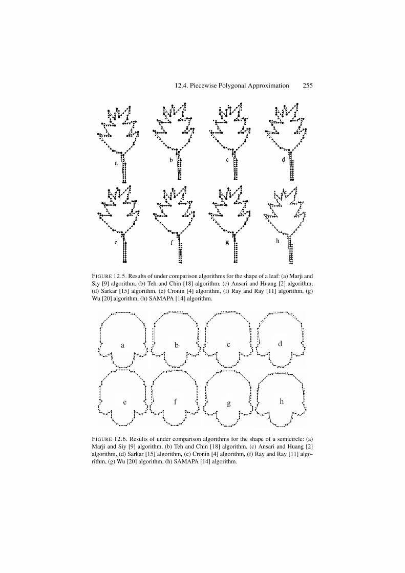
12.4. Piecewise Polygonal Approximation 255
FIGURE 12.5. Results of under comparison algorithms for the shape of a leaf: (a) Marji andSiy [9] algorithm, (b) Teh and Chin [18] algorithm, (c) Ansari and Huang [2] algorithm,(d) Sarkar [15] algorithm, (e) Cronin [4] algorithm, (f) Ray and Ray [11] algorithm, (g)Wu [20] algorithm, (h) SAMAPA [14] algorithm.
a b c d
hgfe
FIGURE 12.6. Results of under comparison algorithms for the shape of a semicircle: (a)Marji and Siy [9] algorithm, (b) Teh and Chin [18] algorithm, (c) Ansari and Huang [2]algorithm, (d) Sarkar [15] algorithm, (e) Cronin [4] algorithm, (f) Ray and Ray [11] algo-rithm, (g) Wu [20] algorithm, (h) SAMAPA [14] algorithm.
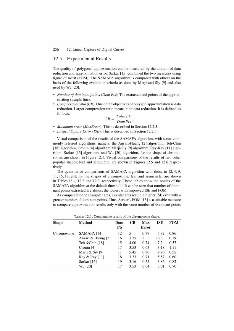
256 12. Linear Capture of Digital Curves
12.5 Experimental Results
The quality of polygonal approximation can be measured by the amount of datareduction and approximation error. Sarkar [15] combined the two measures usingfigure of merit (FOM). The SAMAPA algorithm is compared with others on thebasis of the following evaluation criteria as done by Marji and Siy [9] and alsoused by Wu [20]:
• Number of dominant points (Dom Pts): The extracted end points of the approx-imating straight lines.
• Compression ratio (CR): One of the objectives of polygon approximation is datareduction. Larger compression ratio means high data reduction. It is defined asfollows:
C R = T otal PtsDom Pts
.
• Maximum error (MaxError): This is described in Section 12.2.3.• Integral Square Error (ISE): This is described in Section 12.2.3.
Visual comparison of the results of the SAMAPA algorithm, with some com-monly referred algorithms, namely, the Ansari-Huang [2] algorithm, Teh-Chin[18] algorithm, Cronin [4] algorithm Marji-Siy [9] algorithm, Ray-Ray [11] algo-rithm, Sarkar [15] algorithm, and Wu [20] algorithm, for the shape of chromo-somes are shown in Figure 12.4. Visual comparisons of the results of two otherpopular shapes, leaf and semicircle, are shown in Figures 12.5 and 12.6 respec-tively.
The quantitative comparisons of SAMAPA algorithm with those in [2, 4, 9,11, 15, 18, 20], for the shapes of chromosome, leaf and semicircle, are shownin Tables 12.1, 12.2 and 12.3, respectively. These tables show the results of theSAMAPA algorithm at the default threshold. It can be seen that number of domi-nant points extracted are almost the lowest with improved ISE and FOM.
As compared to the straighter arcs, circular arcs result in higher ISE even with agreater number of dominant points. Thus, Sarkar’s FOM [15] is a suitable measureto compare approximation results only with the same number of dominant points
TABLE 12.1. Comparative results of the chromosome shape.
Shape Method Dom CR Max ISE FOMPts Error
Chromosome SAMAPA [14] 12 5 0.79 5.82 0.86Ansari & Huang [2] 16 3.75 2 20.3 0.19Teh &Chin [18] 15 4.00 0.74 7.2 0.57Cronin [4] 17 3.53 0.63 3.18 1.11Marji & Siy [9] 11 5.45 0.90 9.96 0.55Ray & Ray [11] 18 3.33 0.71 5.57 0.60Sarkar [15] 19 3.16 0.55 3.86 0.82Wu [20] 17 3.53 0.64 5.01 0.70
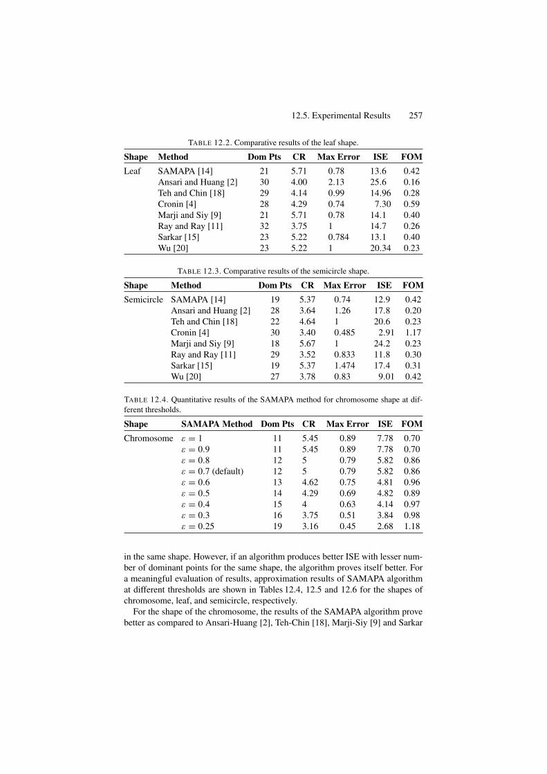
12.5. Experimental Results 257
TABLE 12.2. Comparative results of the leaf shape.
Shape Method Dom Pts CR Max Error ISE FOMLeaf SAMAPA [14] 21 5.71 0.78 13.6 0.42
Ansari and Huang [2] 30 4.00 2.13 25.6 0.16Teh and Chin [18] 29 4.14 0.99 14.96 0.28Cronin [4] 28 4.29 0.74 7.30 0.59Marji and Siy [9] 21 5.71 0.78 14.1 0.40Ray and Ray [11] 32 3.75 1 14.7 0.26Sarkar [15] 23 5.22 0.784 13.1 0.40Wu [20] 23 5.22 1 20.34 0.23
TABLE 12.3. Comparative results of the semicircle shape.
Shape Method Dom Pts CR Max Error ISE FOMSemicircle SAMAPA [14] 19 5.37 0.74 12.9 0.42
Ansari and Huang [2] 28 3.64 1.26 17.8 0.20Teh and Chin [18] 22 4.64 1 20.6 0.23Cronin [4] 30 3.40 0.485 2.91 1.17Marji and Siy [9] 18 5.67 1 24.2 0.23Ray and Ray [11] 29 3.52 0.833 11.8 0.30Sarkar [15] 19 5.37 1.474 17.4 0.31Wu [20] 27 3.78 0.83 9.01 0.42
TABLE 12.4. Quantitative results of the SAMAPA method for chromosome shape at dif-ferent thresholds.
Shape SAMAPA Method Dom Pts CR Max Error ISE FOMChromosome ε = 1 11 5.45 0.89 7.78 0.70
ε = 0.9 11 5.45 0.89 7.78 0.70ε = 0.8 12 5 0.79 5.82 0.86ε = 0.7 (default) 12 5 0.79 5.82 0.86ε = 0.6 13 4.62 0.75 4.81 0.96ε = 0.5 14 4.29 0.69 4.82 0.89ε = 0.4 15 4 0.63 4.14 0.97ε = 0.3 16 3.75 0.51 3.84 0.98ε = 0.25 19 3.16 0.45 2.68 1.18
in the same shape. However, if an algorithm produces better ISE with lesser num-ber of dominant points for the same shape, the algorithm proves itself better. Fora meaningful evaluation of results, approximation results of SAMAPA algorithmat different thresholds are shown in Tables 12.4, 12.5 and 12.6 for the shapes ofchromosome, leaf, and semicircle, respectively.
For the shape of the chromosome, the results of the SAMAPA algorithm provebetter as compared to Ansari-Huang [2], Teh-Chin [18], Marji-Siy [9] and Sarkar
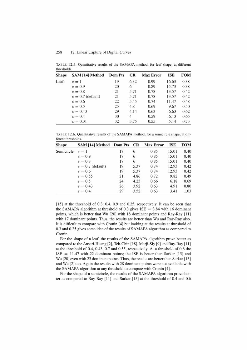
258 12. Linear Capture of Digital Curves
TABLE 12.5. Quantitative results of the SAMAPA method, for leaf shape, at differentthresholds.
Shape SAM [14] Method Dom Pts CR Max Error ISE FOMLeaf ε = 1 19 6.32 0.99 16.63 0.38
ε = 0.9 20 6 0.89 15.73 0.38ε = 0.8 21 5.71 0.78 13.57 0.42ε = 0.7 (default) 21 5.71 0.78 13.57 0.42ε = 0.6 22 5.45 0.74 11.47 0.48ε = 0.5 25 4.8 0.69 9.67 0.50ε = 0.43 29 4.14 0.63 6.63 0.62ε = 0.4 30 4 0.59 6.13 0.65ε = 0.31 32 3.75 0.55 5.14 0.73
TABLE 12.6. Quantitative results of the SAMAPA method, for a semicircle shape, at dif-ferent thresholds.
Shape SAM [14] Method Dom Pts CR Max Error ISE FOMSemicircle ε = 1 17 6 0.85 15.01 0.40
ε = 0.9 17 6 0.85 15.01 0.40ε = 0.8 17 6 0.85 15.01 0.40ε = 0.7 (default) 19 5.37 0.74 12.93 0.42ε = 0.6 19 5.37 0.74 12.93 0.42ε = 0.55 21 4.86 0.72 9.82 0.49ε = 0.5 24 4.25 0.66 6.18 0.69ε = 0.43 26 3.92 0.63 4.91 0.80ε = 0.4 29 3.52 0.63 3.41 1.03
[15] at the threshold of 0.3, 0.4, 0.9 and 0.25, respectively. It can be seen thatthe SAMAPA algorithm at threshold of 0.3 gives ISE = 3.84 with 16 dominantpoints, which is better that Wu [20] with 18 dominant points and Ray-Ray [11]with 17 dominant points. Thus, the results are better than Wu and Ray-Ray also.It is difficult to compare with Cronin [4] but looking at the results at threshold of0.3 and 0.25 gives some idea of the results of SAMAPA algorithm as compared toCronin.
For the shape of a leaf, the results of the SAMAPA algorithm prove better ascompared to the Ansari-Huang [2], Teh-Chin [18], Marji-Siy [9] and Ray-Ray [11]at the threshold of 0.4, 0.43, 0.7 and 0.55, respectively. At a threshold of 0.6 theISE = 11.47 with 22 dominant points; the ISE is better than Sarkar [15] andWu [20] even with 23 dominant points. Thus, the results are better than Sarkar [15]and Wu [2] too. Again the results with 28 dominant points were not available withthe SAMAPA algorithm at any threshold to compare with Cronin [4].
For the shape of a semicircle, the results of the SAMAPA algorithm prove bet-ter as compared to Ray-Ray [11] and Sarkar [15] at the threshold of 0.4 and 0.6
12.6. Optimal Algorithms 259
respectively. The results also prove better with even lesser number of dominantpoints than Ansari-Huang [2], Teh-Chin [18], Marji-Siy [9] and Wu [20] at thresh-old of 0.3, 0.55, 0.8, and 0.43. The results of the SAMAPA algorithm at thresholdof 0.3 and Cronin [4] are the same. The algorithm by Cronin [4] looks to performbetter in all three shapes but it can be seen that the number of dominant pointsdetected by Cronin are always larger.
Another additional advantage of the SAMAPA algorithm is its computationalefficiency. Break points are selected in the start and only these points, as candi-date end points of approximating straight lines, are considered during the furtherprocessing of polygonal approximation algorithm. As the given curve is dividedinto pieces and processing of each piece of curve is independent from other pieces;therefore parallel processing can be applied.
12.6 Optimal Algorithms
Polygonal approximation is a common and efficient representation of digitalcurves. A problem with natural interest is the detection of optimal polygonalapproximation. Optimal approaches tend to find the optimal polygonal approxima-tion based on specified criteria and error-bound constraints. One desired criterionfor optimality is approximation with minimal number of vertices, distant fromthe original curve by no more than a prespecified value. The optimal polygonalapproximation is formulated as an optimization problem, which seeks to minimizethe error measure of fitness by locating a given number of vertices. This problemcan be solved by using a dynamic programming [4, 8, 73, 74], A∗, search [75], orby algorithms developed for the shortest-path problem in digraph [76–78].
12.6.1 Dynamic ProgrammingThe problem of polygonal approximation of digital curves is stated as follows:given a digital curve of N points, find M vertices amount them so that the polygonconstructed by directly connecting these vertices best fits the given digital curve.The set of N given points is denoted by
S = {s1, s2, . . . , sN } = {(xs1, ys
1), (xs2, ys
2), . . . , (xsN , ys
N )}, (12.23)
The set of M vertices to be found among S is denoted by
V = {v1, v2, . . . , vM } = {(xv1 , yv
1 ), (xv2 , yv
2 ), . . . , (xvM , yv
M )}, (12.24)
The fitting error of the kth edge is denoted by e(vk, vk+1), which is the sumof error norms from each point between vk and vk+1 to the corresponding edgevkvk+1. The norm used is the integral square error. The polygonal approximationproblem is formulated as follows: given a point set S of size N , find a subset V ofsize M from S, where v1 = s1 and vM = sN , such that the total error measure is
260 12. Linear Capture of Digital Curves
minimized. That is, we seek to find the minimum error measure as follows:
E(N , M) = minV ⊂S
M−1∑
K=1
e(vk, vk+1). (12.25)
The dynamic programming technique can be applied to find the globally optimalsolution of the above problem. Dynamic programming is an optimization methodthat makes an optimal decision based on all possible previous states with a properrecurrence relation. The following recursive function can be applied to solve thegiven problem:
E(n, m) = minm−1≤ j≤n−1
[E( j, m − 1) + e(s j , sn)], (12.26)
where E(n, m) denotes the minimum error of fitting first n points by using mvertices, E( j, m − 1) denotes the minimization error of fitting first j points byusing m − 1 vertices, and e(s j , sn) denotes the error of fitting the curve segmentbetween s j and sn by a single edge. The value of j ranges from m − 1 to n − 1,which is the possible range of distributing first m − 1 vertices. The principle ofdynamic programming is to derive E(., m) from E(., m − 1) recursively. E(n, m)is found by adjusting j , such that the sum of E( j, m − 1) and s(s j , sn) reachesthe minimum value. This process is initialized with E(1, 1) = 0 and E(n, 1) =+∞ for n = 2, . . ., N ; and is terminated at E(N , M). The number of vertices mmust be smaller than or equal to the number of points n. As a result, the dynamicprogramming fills up the lower triangle of the array E(., .) with size N × M . Thevalue of E(N , M) is the global minimum error of fitting the given digital curve oflength N by using a polygon of M vertices.
12.6.2 Perez and Vidal AlgorithmThe work of Perez and Vidal is based on dynamic programming [8]. It is a well-known approach to define an algorithm that finds optimal results according to aspecific criterion. Perez and Vidal algorithm is described as follows:
g[1, 0] = 0;FOR n = 2 TO NP DO g[n, 0] = MaxReal;(∗arbitrary high value for initialization ∗)FOR m = 1 TO NS DO
FOR n = 2 TO NP DOBEGIN
(∗Search for the minimum error to reach point n with m segments:∗)g[n, m] = Min{ g[i, m − l] + error(i, n)/i ∈ [m, n − l] }Father[n, m] = mini
END;TotalError = g(n, m];
12.6. Optimal Algorithms 261
For a clear understanding of the method, some important variables are presentedas follows:
• g: array[1. . . NP, 0. . . NS] of real; g is used to memorize the minimum globalerror to reach any point of the contour, using any number of segments. Forinstance, g[30, 4] is the minimum global error to reach the 30th point usingfour line segments.
• Points: array[1. . . NP] of RPoint; RPoint is a structure with x and y coordinates.• Father: array[1. . . NP, 1. . . NS] of integer; This array is used to memorize the
starting point of the last segment. For instance, Father[30,4] is the number ofthe starting point of the 4th segment, the 30th being the ending point.
The Perez and Vidal algorithm employs dynamic programming, which has twomajor problems. First, in applying dynamic programming, the number of ver-tices to locate should be assigned a priori. This parameter value is hard to predictsince the suitable number of vertices varies from case to case and depends largelyon the geometric size and features of the given digital curve. Second, the dynamicprogramming is time consuming, especially while dealing with closed curves. Allpossible initial points should be examined to achieve the global minimum fittingerror.
12.6.3 Some Remarks on Optimal AlgorithmsA global optimum is the major advantage of the dynamic programming approach.However, this approach suffers from two severe problems. First, the proper num-ber of vertices is hard to decide a priori. Secondly, the computational complex-ity is much higher than other existing methods. The time complexity of applyingdynamic programming to polygonal approximation is in the order of O(MN3). Themain task is to fill up the array E(.,.) of size N × M .
Each entry of array involves the O(N 2) computation of Equation (12.26). Forfitting close curves, an additional outer loop of size N is required to obtain a properinitial point that minimizes the global fitting error. The overall time complexity ofconstructing optimal polygonal approximation of closed digital curves by order ofO(MN4). Thus, in its present form, applying this algorithm on large digital curvesextracted from real images is impractical.
The problem of finding the minimum error of the best line segment approximat-ing a curve is addressed in optimal algorithm by Perez and Vidal [45]. Unfortu-nately, a mathematical analysis of the error function shows that this minimum ishard to find. However, it is possible to determine a lower-bound on the error. Thevalues of the least-square errors of both regression lines are required. The compu-tation of the lower-bound is given by Salotti [75] and he uses the lower-bound, inhis A∗ algorithm, to speed up the search and reduce the complexity. Various otherimprovements can be found in [4,76–79]. To sum up, the proposed approaches forclosed curves are suboptimal, whereas the optimal choice of the starting point istime-consuming. Thus, the problem still remains unsolved.
262 12. Linear Capture of Digital Curves
12.7 Summary
Capturing with linear/polygonal approximation was covered in this discussion.In addition to providing a general overview of the topic, some algorithmswere described that are subsequently used for comparison with the SAMAPAalgorithm in this chapter. Piecewise polygonal approximation is a split-and-mergetype of technique implemented by a recursive algorithm. Comparative study inSection 12.5 demonstrates that results of the SAMAPA technique are much betterthan for its predecessors.
12.8 Exercises
1. Write a program to implement the Freeman’s chain code method and verify thecode for the test shapes of chromosome, leaf, and semicircle in Figure 12.2.
2. Collect three different test images than those used in this chapter and computetheir chain code using the program of Exercise 12.8.1.
3. Write programs to implement the Teh and Chin, Marji and Siy, Wu, andSAMAPA algorithms described in Sections 12.3–12.4.
4. Test your programs of Exercise 12.8.3 for the test shapes of chromosome, leaf,and semicircle used in this chapter.
5. Test your programs of Exercise 12.8.3 for the test shapes of Exercise 12.8.2.6. Using your program in Exercise 11.10.2, verify the results in Tables 12.1–12.6.
References1. Attneave, F. (1954), Some information aspects of visual perception. Psychol Rev
61:183–193.2. Ansari, N., and Huang. K.W. (1991), Nonparametric dominant points detection. Pat-
tern Recognition 24:849–862, 1991.3. Arcelli, C., and Ramella. G. (1993), Finding contour-based abstractions of planner
patterns. Pattern Recognition 26(10):1563–1577.4. Cronin, T.M. (1999), A boundary concavity code to support dominant points detection,
Pattern Recognition Lett 20, 617–634.5. Dunham. J.G. (1986), Optimum uniform piecewise linear approximation of planner
curves. IEEE Trans Anal Mach Intell 8:67–75.6. Freeman. H. (1061), On the encoding of arbitrary geometric configurations. IRE Trans
Elec Comp 10:260–268.7. Kurozumi, Y., and Davis. W.A. (1982), Polygonal approximation by minimax method.
Comput Graphics Image Process 19:248–264.8. Lowe, D.G. (1987), Three-dimensional object recognition from single two-
dimensional images. AI 31:355–395.9. Marji, M., and Siy, P. (2003), A new algorithm for dominant points detection and
polygonization of digital curves, Pattern Recognition 36, 2239–2251.10. Ramer. U. (1972), An iterative procedure for the polygonal approximation of plane
curves. Comput Graphics Image Process 1:244–256.
References 263
11. Ray, B.K., and Ray, K.S. (1992), Detection of significant points and polygonal approx-imation of digitized curves, Pattern Recognition Lett 13, 443–452.
12. Rosin. P.L. (1998), Assessing the behavior of polygonal approximation algorithms.Ninth British Machine Vision Conference, Southampton, UK.
13. Rosin. P.L. (1997), Techniques for assessing polygonal approximations of curves.IEEE Trans PAMI 19(6):659:666.
14. Sarfraz, M., Asim, M.R., and Masood, A. (2004), Piecewise polygonal approximationof digital curves, The Proceedings of IEEE International Conference on InformationVisualisation (IV’2004)-UK, IEEE Computer Society Press, pp. 991–996.
15. Sarkar, D. (1993), A simple algorithm for detection of significant vertices for polygo-nal approximation of chain-coded curves, Pattern Recognition Lett 14, 959–964.
16. Sato, Y. (1992), Piecewise linear approximation of plane curves by perimeter opti-mization. Pattern Recognition 25:1535–1543.
17. Slansky, J., and Gonazlez. V. (1980), Fast polygonal approximation of digitized curves.Pattern Recognition 12:327–331.
18. The, C., and Chin, R. (1989), On the detection of dominant points on digital curves,IEEE Trans PAMI 8, 859–873.
19. Wang, M.J., Wu, W.Y., Huang, L.K., and Wang. D.M. (1995), Corner detection usingbending value. Pattern Recognition Lett 16:575–583.
20. Wu, W.Y. (2003), An adaptive method for detecting dominant points, Pattern Recog-nition 36, 2231–2237.
21. Yin. P.Y. (2003), Ant colony search algorithms for optimal polygonal approximationof plane curves. Pattern Recognition 36:1783–1797.
22. Melkman, A., and Rourke, J.O. (1988), On polygonal chain approximation. Proceed-ings of Computational Morphology, North-Holland, Amsterdam, pp. 87–95.
23. Sklansky, J., and Gonzalez, V. (1980), Fast polygonal approximation of digitizedcurves, Pattern Recognition 12, 327–331.
24. Held, A., Abe, K., and Arcelli, C. (1994), Towards a hierarchical contour descriptionvia dominant point detection, IEEE Trans Sys Man Cybernetics 24, 942–949.
25. Dunham, J.G. (1986), Optimum uniform piecewise linear approximation of planarcurves, IEEE Trans PAMI 8, 67–75.
26. Sato, Y. (1992), Piecewise linear approximation of plane curves by perimeter opti-mization, Pattern Recognition 25, 1535–1543.
27. Goldberg, D.E. (1989), Genetic Algorithms in Search Optimization and MachineLearning, Addison-Wesley, Reading, MA,.
28. Huang, S.C., and Sun, Y.N. (1999), Polygonal approximation using genetic algorithms,Pattern Recognition 32, 1409–1420.
29. Pal, N.R., Nandi, S., and Kundu, M.K. (1998), Self-crossover: a new genetic operatorand its application to feature selection. Int J Systems Sci 2, 207–212.
30. Yin, P.Y. (1999), Genetic algorithms for polygonal approximation of digital curves, IntJ Pattern Recognition Artif Intell 13, 1–22.
31. Yin, P.Y. (2000), A tabu search approach to the polygonal approximation of digitalcurves, Int J Pattern Recognition Artif Intell 14, 243–255.
32. Yin, P.Y. (2003), Ant colony search algorithms for optimal polygonal approximationof plane curves, Pattern Recognition, 36, 1783–1797.
33. Davis, L.S. (1977), Understanding shape angles and sides, IEEE Trans Comput 26,236–242.
34. Sankar, P.V., and Sharma, C.V. (1978), A parallel procedure for the detection of dom-inant points on digital curve, Comput Graphics Image Process 7, 403–412.

264 12. Linear Capture of Digital Curves
35. Latecki, L.J., and Lakamper, R. (1999), Convexity rule for shape decomposition basedon discrete contour evolution, Comput Vision Image Understanding 73, 441–454.
36. Latecki, L.J., Ghadially, R.R., Lakamper, R., and Eckhardt, U. (2000), Continuity ofthe discrete curve evolution, J Electronic Imaging 9, 317–326.
37. Sankar, P.V., and Sharma, C.V. (1978), A parallel procedure for the detection of dom-inant points on digital curve, Comput Graphics Image Process 7, 403–412.
38. Latecki, L.J., and Lakamper, R. (1999), Convexity rule for shape decomposition basedon discrete contour evolution, Comput Vision Image Understanding 73, 441–454.
39. Latecki, L.J., Ghadially, R.R., Lakamper, R., and Eckhardt, U. (2000), Continuity ofthe discrete curve evolution, J Electronic Imaging 9, 317–326.
40. Rosenfeld, A., and Weszka, J.S. (1975), An improved method of angle detection ondigital curves, IEEE Trans Comput 24, 940–941.
41. Rosenfeld, A. Johnston, E. (1973), Angle detection on digital curves, IEEE TransComput 22, 875–878.
42. Freeman, H., and Davis, L.S. (1977), A corner-finding algorithm for chain-codedcurves, IEEE Trans Comput 26, 297–303.
43. Neumann, R., and Teisseron, G. (2002), Extraction of dominant points by estimationof the contour fluctuations, Pattern Recognition 35, 1447–1462.
44. Lowe, D.G. (1987), Three-dimensional object recognition from single two-dimensional images, Artific Intell 31, 355–395.
45. Perez, J.C., and Vidal, E. (1994), Optimum polygonal approximation of digitizedcurves, Pattern Recognition Lett 15, 743–750.
46. Chan, W.S., and Chin, F. (1996), On approximation of polygonal curves with minimumnumber of line segments or minimum error, Int J Comput Geom Appl 6, 59–77.
47. Saghri, J., and Freeman, H. (1981), Analysis of the precision of generalized chaincodes for the representation of planar curves, IEEE Trans PAMI 3, 533–539.
48. Koplowitz, J. (1981), On the performance of chain codes for quantization of the linedrawings. IEEE Trans PAMI 3, 180–185.
49. Li, L. Chen, W. (1999), Corner detection and interpretation on planar curves usingfuzzy reasoning, IEEE Trans PAMI, 21, 1204–1210.
50. Kaneko, T., and Okudaira, M. (1985), Encoding of arbitrary curves based on the chaincode representation, IEEE Trans Comm 33, 697–707.
51. Kurozumi, Y., and Davis, W.A. (1982), Polygonal approximation by the minimaxmethod, Comput Graphics Image Process 19, 248–264.
52. Pikaz, A., and Dinstein, I. (1995), An algorithm for polygonal approximation of digitalcurves based on iterative points elimination, Pattern Recognition Lett 16, 557–563.
53. Leu, J.G., and Chen, L. (1988), Polygonal approximation of 2-D shapes throughboundary merging, Pattern Recognition, 28, 571–579.
54. Ray, B.K., and Ray, K.S. (1995), A new split-and-merge technique for polygonalapproximation of chain coded curves, Pattern Recognition Lett 16, 161–169.
55. Inesta, J.M., Buendia, M., and Sarti, M.A. (1988), Reliable polygonal approxima-tions of imaged real objects through dominant point detection, Pattern Recognition 31,685–697.
56. Yin, P.Y. (1998), Algorithms for straight-line fitting using K -means, Pattern Recogni-tion Lett 19, 31–41.
57. Yukio, S. (1992), Piecewise linear approximation of plane curves by perimeter opti-mization, Pattern Recognition, 25, 1535–1543.
58. Imai, H., and Iri, M. (1986), Computational-geometric methods for polygonal approx-imations of a curve, Comp Vis Image Proc 36, 31–41.
References 265
59. Leymarie, F., and Levine, M.D. (1988), Curvature Morphology, Center of IntelligentMachines, TR-CIM-88-26, McGill University, Montreal.
60. Ray, B.K., and Ray, K.S. (1992), An algorithm for detecting dominant points andpolygonal approximation of digitized curves, Pattern Recognition Lett 13, 849–856.
61. Zhang, X., and Zhao, D. (1997), A parallel algorithm for detecting dominant points onmultiple digital curves, Pattern Recognition, 30, 239–244.
62. Cheng, K.H., and Hsu W.H., (1988), Parallel algorithms for corner following on digitalcurves, Pattern Recognition Lett 8, 47–53.
63. Phillips, T.Y., and Rosenfeld, A. (1987), A method for curve partitioning using arc-chord distance, Pattern Recognition Lett 5, 285–288.
64. Fischler, M.A., and Wolf, H.C. (1994), Locating perceptually salient points on planarcurves, IEEE Trans. PAMI 16, 113–129.
65. Han, J.H., and Poston, T. (2001), Chord-to-point distance accumulation and planarcurvature: a new approach to discrete curvature, Pattern Recognition Lett 22,1133–1144.
66. Ogawa, H. (1989), Corner detection on digital curves based on local symmetry of theshape, Pattern Recognition, 22, 351–357.
67. Ansari, N., and Huang, K.W. (1991), Nonparametric dominant point detection, PatternRecognition, 24, 849–862.
68. Koplowitz, J., and Plante, S. (1995), Corner detection for chain coded curves, PatternRecognition 28, 843–852.
69. Tsai, D.M. (1997), Boundary-based corner detection using neural networks, PatternRecognition 30, 85–97.
70. Lee, J.S., Sun, Y.N., Chen, C.H., and Tsai, C.T. (1993), Wavelet-based corner detec-tion, Pattern Recognition, 26, 853–865.
71. Quddus, A., and Fahmy, M.M. (1999), Fast wavelet-based corner detection technique,Electron Lett 35, 287–288.
72. Pikaz, A., and Dinstein, I. (1995), Optimal polygonal approximation of digital curves,Pattern Recognition 28, 373–279.
73. Horng, J.H., and Li, J.T. (2002), An automatic and efficient dynamic programmingalgorithm for polygonal approximation of digital curves, Pattern Recognition Lett 23,171–182.
74. Kolesnikov, A., and Franti, P. (2003), Reduced search dynamic programming forapproximation of polygonal curves, Pattern Recognition Lett 24, pp. 2243–2254.
75. Salotti, M. (2000), Improvement of Perez and Vidal algorithm for the decomposition ofdigitized curves into line segments, 15th International Conference on Pattern Recog-nition, Vol. 2, pp. 878–882.
76. Zhu, Y., and Seneviratne, L.D (1997), Optimal polygonal approximation of digitizedcurves. IEE Proc. of Vision, Image and Signal Processing, Vol. 144, pp. 8–14.
77. Chan, W.S., and Chin, F. (1996), On approximation of polygonal curves with minimumnumber of line segments or minimum error, Int J Comput Geom Appl 6, 59–77.
78. Kolesnikov, A., and Franti, P. (2005), Min-# polygonal approximation of closedcurves, IEEE International Conference on Image Processing, Vol. 2, pp. 522–525.
79. Horng, J.H. (2002), Improving fitting quality of polygonal approximation by using thedynamic programming technique, Pattern Recognition Lett 23, 1657–1673.
13Digital Outline Capture with CubicCurves
Abstract. In this chapter, an automatic and efficient algorithm for outline capture ofcharacter images, stored as bitmaps, is presented. This method is well suited for charactersof non-Roman languages such as Arabic, Japanese, Urdu, Persian, and so on. Contem-porary word processing systems store shapes of characters in terms of their outlines, andoutlines are expressed as cubic Bezier curves. The process of capturing outlines includesvarious steps including detection of the boundary, finding corner points and break points,and fitting the curve. The chapter discusses automating the above process to provide opti-mal results. As an alternate smoother scheme, the Hermite cubic spline curve scheme hasalso been introduced.
13.1 Introduction
Fonts are an essential part of any computer system. Two fundamental approachesto storing fonts on a computer are bitmap and outline [1, 2]. In bitmap fonts, eachcharacter is stored as an array of pixels (a bitmap). Outline fonts describe thecharacter outlines [18–29] with a combination of control points and curves. Out-line representation has many advantages over the bitmap approach such as scaling,shearing, translation, rotation, and clipping. Therefore, most contemporary desk-top publishing systems are based on outline fonts.
Characters of non-Roman languages are complex and their cursive naturerequires much more attention. In traditional font design, a character is drawn ini-tially on paper by hand and then it is scanned to obtain a gray-level image. Fromthis gray-level image, the boundary, or contour, of the character is obtained. Thencorner points of the character are determined from the contour. These cornerpoints can be obtained by some interactive method or by some automated cornerdetection algorithm [3,4]. Curve fitting is done by segmenting the boundary at thecorner points and fitting the parametric curve to these points.
This chapter includes an automatic algorithm [18] to obtain the outline ofbitmap characters. The algorithm presented improves the work done in [5,6]. Themethodology adopted in this chapter gives a higher level of accuracy and speed
267
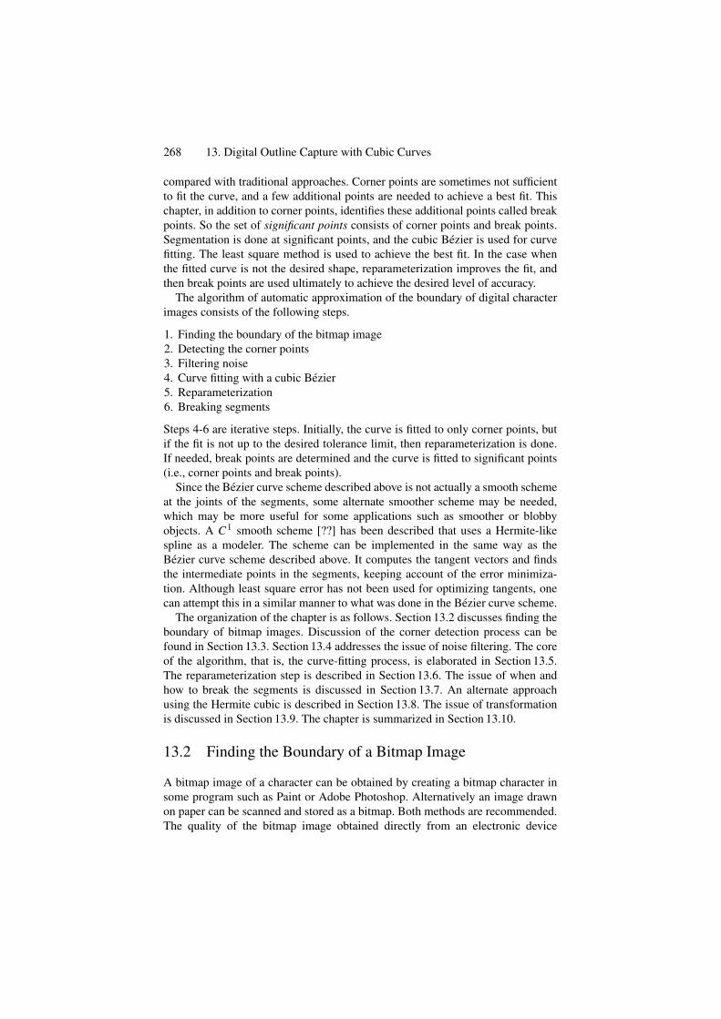
268 13. Digital Outline Capture with Cubic Curves
compared with traditional approaches. Corner points are sometimes not sufficientto fit the curve, and a few additional points are needed to achieve a best fit. Thischapter, in addition to corner points, identifies these additional points called breakpoints. So the set of significant points consists of corner points and break points.Segmentation is done at significant points, and the cubic Bezier is used for curvefitting. The least square method is used to achieve the best fit. In the case whenthe fitted curve is not the desired shape, reparameterization improves the fit, andthen break points are used ultimately to achieve the desired level of accuracy.
The algorithm of automatic approximation of the boundary of digital characterimages consists of the following steps.
1. Finding the boundary of the bitmap image2. Detecting the corner points3. Filtering noise4. Curve fitting with a cubic Bezier5. Reparameterization6. Breaking segments
Steps 4-6 are iterative steps. Initially, the curve is fitted to only corner points, butif the fit is not up to the desired tolerance limit, then reparameterization is done.If needed, break points are determined and the curve is fitted to significant points(i.e., corner points and break points).
Since the Bezier curve scheme described above is not actually a smooth schemeat the joints of the segments, some alternate smoother scheme may be needed,which may be more useful for some applications such as smoother or blobbyobjects. A C1 smooth scheme [??] has been described that uses a Hermite-likespline as a modeler. The scheme can be implemented in the same way as theBezier curve scheme described above. It computes the tangent vectors and findsthe intermediate points in the segments, keeping account of the error minimiza-tion. Although least square error has not been used for optimizing tangents, onecan attempt this in a similar manner to what was done in the Bezier curve scheme.
The organization of the chapter is as follows. Section 13.2 discusses finding theboundary of bitmap images. Discussion of the corner detection process can befound in Section 13.3. Section 13.4 addresses the issue of noise filtering. The coreof the algorithm, that is, the curve-fitting process, is elaborated in Section 13.5.The reparameterization step is described in Section 13.6. The issue of when andhow to break the segments is discussed in Section 13.7. An alternate approachusing the Hermite cubic is described in Section 13.8. The issue of transformationis discussed in Section 13.9. The chapter is summarized in Section 13.10.
13.2 Finding the Boundary of a Bitmap Image
A bitmap image of a character can be obtained by creating a bitmap character insome program such as Paint or Adobe Photoshop. Alternatively an image drawnon paper can be scanned and stored as a bitmap. Both methods are recommended.The quality of the bitmap image obtained directly from an electronic device
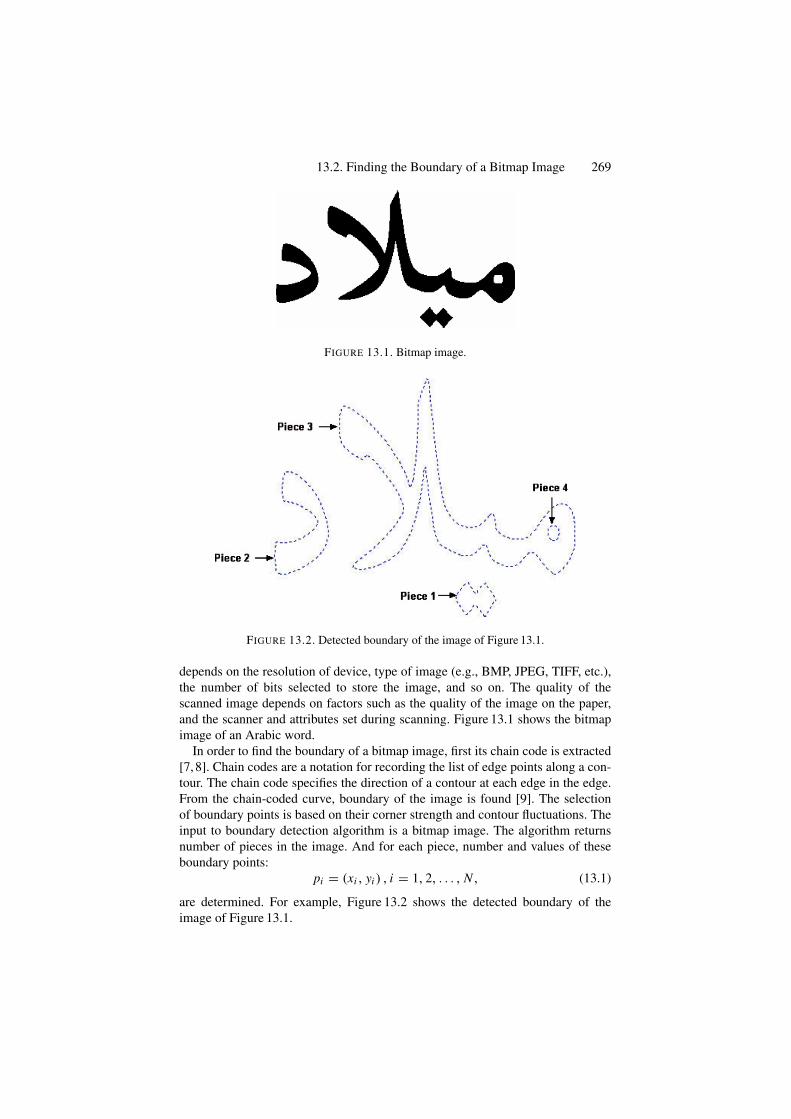
13.2. Finding the Boundary of a Bitmap Image 269
FIGURE 13.1. Bitmap image.
FIGURE 13.2. Detected boundary of the image of Figure 13.1.
depends on the resolution of device, type of image (e.g., BMP, JPEG, TIFF, etc.),the number of bits selected to store the image, and so on. The quality of thescanned image depends on factors such as the quality of the image on the paper,and the scanner and attributes set during scanning. Figure 13.1 shows the bitmapimage of an Arabic word.
In order to find the boundary of a bitmap image, first its chain code is extracted[7,8]. Chain codes are a notation for recording the list of edge points along a con-tour. The chain code specifies the direction of a contour at each edge in the edge.From the chain-coded curve, boundary of the image is found [9]. The selectionof boundary points is based on their corner strength and contour fluctuations. Theinput to boundary detection algorithm is a bitmap image. The algorithm returnsnumber of pieces in the image. And for each piece, number and values of theseboundary points:
pi = (xi , yi ) , i = 1, 2, . . . , N , (13.1)
are determined. For example, Figure 13.2 shows the detected boundary of theimage of Figure 13.1.
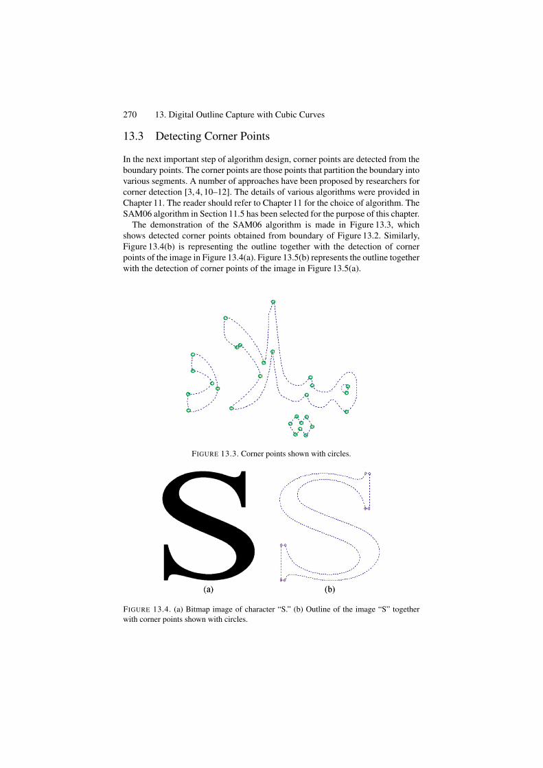
270 13. Digital Outline Capture with Cubic Curves
13.3 Detecting Corner Points
In the next important step of algorithm design, corner points are detected from theboundary points. The corner points are those points that partition the boundary intovarious segments. A number of approaches have been proposed by researchers forcorner detection [3, 4, 10–12]. The details of various algorithms were provided inChapter 11. The reader should refer to Chapter 11 for the choice of algorithm. TheSAM06 algorithm in Section 11.5 has been selected for the purpose of this chapter.
The demonstration of the SAM06 algorithm is made in Figure 13.3, whichshows detected corner points obtained from boundary of Figure 13.2. Similarly,Figure 13.4(b) is representing the outline together with the detection of cornerpoints of the image in Figure 13.4(a). Figure 13.5(b) represents the outline togetherwith the detection of corner points of the image in Figure 13.5(a).
FIGURE 13.3. Corner points shown with circles.
FIGURE 13.4. (a) Bitmap image of character “S.” (b) Outline of the image “S” togetherwith corner points shown with circles.
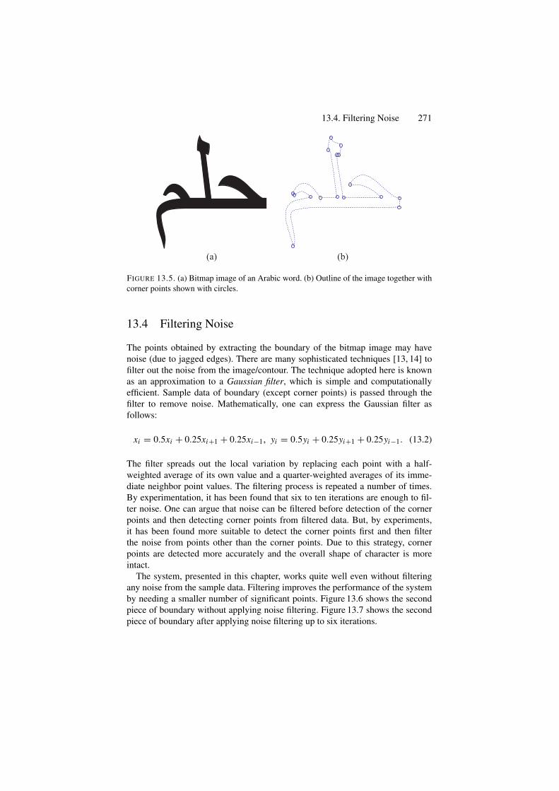
13.4. Filtering Noise 271
(a) (b)
FIGURE 13.5. (a) Bitmap image of an Arabic word. (b) Outline of the image together withcorner points shown with circles.
13.4 Filtering Noise
The points obtained by extracting the boundary of the bitmap image may havenoise (due to jagged edges). There are many sophisticated techniques [13, 14] tofilter out the noise from the image/contour. The technique adopted here is knownas an approximation to a Gaussian filter, which is simple and computationallyefficient. Sample data of boundary (except corner points) is passed through thefilter to remove noise. Mathematically, one can express the Gaussian filter asfollows:
xi = 0.5xi + 0.25xi+1 + 0.25xi−1, yi = 0.5yi + 0.25yi+1 + 0.25yi−1. (13.2)
The filter spreads out the local variation by replacing each point with a half-weighted average of its own value and a quarter-weighted averages of its imme-diate neighbor point values. The filtering process is repeated a number of times.By experimentation, it has been found that six to ten iterations are enough to fil-ter noise. One can argue that noise can be filtered before detection of the cornerpoints and then detecting corner points from filtered data. But, by experiments,it has been found more suitable to detect the corner points first and then filterthe noise from points other than the corner points. Due to this strategy, cornerpoints are detected more accurately and the overall shape of character is moreintact.
The system, presented in this chapter, works quite well even without filteringany noise from the sample data. Filtering improves the performance of the systemby needing a smaller number of significant points. Figure 13.6 shows the secondpiece of boundary without applying noise filtering. Figure 13.7 shows the secondpiece of boundary after applying noise filtering up to six iterations.
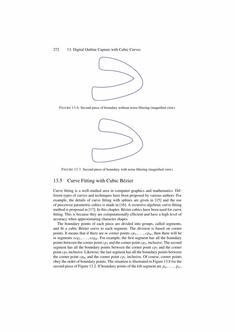
272 13. Digital Outline Capture with Cubic Curves
FIGURE 13.6. Second piece of boundary without noise filtering (magnified view).
FIGURE 13.7. Second piece of boundary with noise filtering (magnified view).
13.5 Curve Fitting with Cubic Bezier
Curve fitting is a well-studied area in computer graphics and mathematics. Dif-ferent types of curves and techniques have been proposed by various authors. Forexample, the details of curve fitting with splines are given in [15] and the useof piecewise parametric cubics is made in [16]. A recursive algebraic curve-fittingmethod is proposed in [17]. In this chapter, Bezier cubics have been used for curvefitting. This is because they are computationally efficient and have a high level ofaccuracy when approximating character shapes.
The boundary points of each piece are divided into groups, called segments,and fit a cubic Bezier curve to each segment. The division is based on cornerpoints. It means that if there are m corner points cp1, . . . , cpm , then there will bem segments seg1, . . . , segm . For example, the first segment has all the boundarypoints between the corner point cp1 and the corner point cp2, inclusive. The secondsegment has all the boundary points between the corner point cp2 and the cornerpoint cp3 inclusive. Likewise, the last segment has all the boundary points betweenthe corner point cpm and the corner point cp1 inclusive. Of course, corner pointsobey the order of boundary points. The situation is illustrated in Figure 13.8 for thesecond piece of Figure 13.2. If boundary points of the kth segment are pu, . . . , pw,
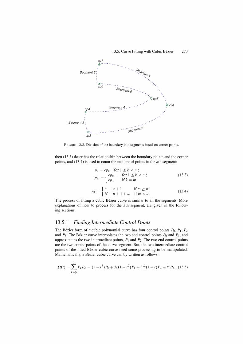
13.5. Curve Fitting with Cubic Bezier 273
Segment 6
cp1
cp4
cp6
cp3
cp5
cp2
Segment 5
Segment 4
Segment 3
Segment 2
Segment 1
FIGURE 13.8. Division of the boundary into segments based on corner points.
then (13.3) describes the relationship between the boundary points and the cornerpoints, and (13.4) is used to count the number of points in the kth segment:
pu = cpk for 1 ≤ k < m;pw =
{cpk+1 for 1 ≤ k < m;cp1 if k = m.
(13.3)
nk ={
w − u + 1 if w ≥ u;N − u + 1 + w if w < u.
(13.4)
The process of fitting a cubic Bezier curve is similar to all the segments. Moreexplanations of how to process for the kth segment, are given in the follow-ing sections.
13.5.1 Finding Intermediate Control PointsThe Bezier form of a cubic polynomial curve has four control points P0, P1, P2and P3. The Bezier curve interpolates the two end control points P0 and P3, andapproximates the two intermediate points, P1 and P2. The two end control pointsare the two corner points of the curve segment. But, the two intermediate controlpoints of the fitted Bezier cubic curve need some processing to be manipulated.Mathematically, a Bezier cubic curve can by written as follows:
Q(t) =3∑
k=0
Pk Bk = (1 − t3)P0 + 3t (1 − t2)P1 + 3t2(1 − t)P2 + t3 P3, (13.5)
274 13. Digital Outline Capture with Cubic Curves
where 0 ≤ t ≤ 1, P0 = pu, P3 = pw for the kth segment, the boundary points ofwhich are pu, . . . , pw. Let
Pi = (Pxi , Pyi ),
andQ(t) = (Qx (t), Qy(t)),
then (13.5) can be expressed as follows:
Qx (t) = (1 − t3)Px0 + 3t (1 − t2)Px1 + 3t2(1 − t)Px2 + t3 Px3, (13.6)
Qy(t) = (1 − t3)Py0 + 3t (1 − t2)Py1 + 3t2(1 − t)Py2 + t3 Py3 . (13.7)
As far as parameterization is concerned, the choice of chord-length parameteri-zation has been adopted. Thus, the parametric value t , associated with each pointpi , can be to estimated as follows:
ti =
⎧⎪⎪⎨
⎪⎪⎩
0, if i = u;|pu pu+1| + |pu+1 pu+2| + · · · + |pi−1 pi ||pu pu+1| + |pu+1 pu+2| + · · · + |pw−1 pw| , for u + 1 ≤ i ≤ w − 1;1, if i = w.
(13.8)It is obvious that the number of points in the kth segment (i.e., nk) and the numberof t values associated with them are same.
The goal here is to approximate the boundary of the original image by a para-metric curve in an optimal way. To achieve this goal, one needs to find the valuesof P1 and P2 that minimize the distance between the boundary and parametriccurve. For this purpose, the least square method has been used. That is, one candefine the sum of squared distances S from the boundary to the parametric curve.Mathematically, it can be expressed as follows:
S =w∑
i=u
[Qi (t) − pi ]2,
=w∑
i=u
[Qxi (t) − pxi ]2+w∑
i=u
[Qyi (t) − pyi ]2.
(13.9)
The goal is to minimize S. It is required to find partial derivatives of (13.9) withrespect to P1 and P2 and equate them to zero as follows:
∂S∂ P1
= 0, (13.10)
∂S∂ P2
= 0. (13.11)
The solution will provide the values of P1 and P2 that approximate the boundaryby a parametric curve in the best way for given values of t . Now, manipulatingEquation (13.15) yields the following:
∂S∂ P1
= 2w∑
i=u
∂ Q(ti )∂ P1
[Q(ti ) − pi ] = 0,
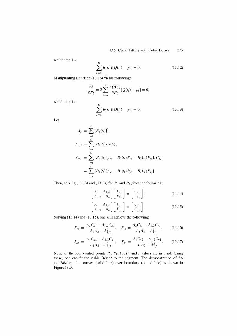
13.5. Curve Fitting with Cubic Bezier 275
which impliesw∑
i=u
B1(ti )[Q(ti ) − pi ] = 0. (13.12)
Manipulating Equation (13.16) yields following:
∂S∂ P2
= 2w∑
i=u
∂ Q(ti )∂ P2
[Q(ti ) − pi ] = 0,
which impliesw∑
i=u
B2(ti )[Q(ti ) − pi ] = 0. (13.13)
Let
Ak =w∑
i=u
[Bk(ti )]2,
A1,2 =w∑
i=u
[B1(ti )B2(ti ),
Cxk =w∑
i=u
[Bk(ti )[pxi − B0(ti )Px0 − B3(ti )Px3], Cyk
=w∑
i=u
[Bk(ti )[pyi − B0(ti )Py0 − B3(ti )Py3].
Then, solving (13.13) and (13.13) for P1 and P2 gives the following:[
A1 A1,2A1,2 A2
] [Px1
Px2
]=[
Cx1
Cx2
], (13.14)
[A1 A1,2A1,2 A2
] [Py1
Py2
]=[
Cy1
Cy2
]. (13.15)
Solving (13.14) and (13.15), one will achieve the following:
Px1 = A2Cx1 − A1,2Cx2
A1 A2 − A21,2
, Py1 = A2Cy1 − A1,2Cy2
A1 A2 − A21,2
, (13.16)
Px2 = A1Cx2 − A1,2Cx1
A1 A2 − A21,2
, Py2 = A1Cy2 − A1,2Cy1
A1 A2 − A21,2
. (13.17)
Now, all the four control points P0, P1, P2, P3 and t values are in hand. Usingthese, one can fit the cubic Bezier to the segment. The demonstration of fit-ted Bezier cubic curves (solid line) over boundary (dotted line) is shown inFigure 13.9.
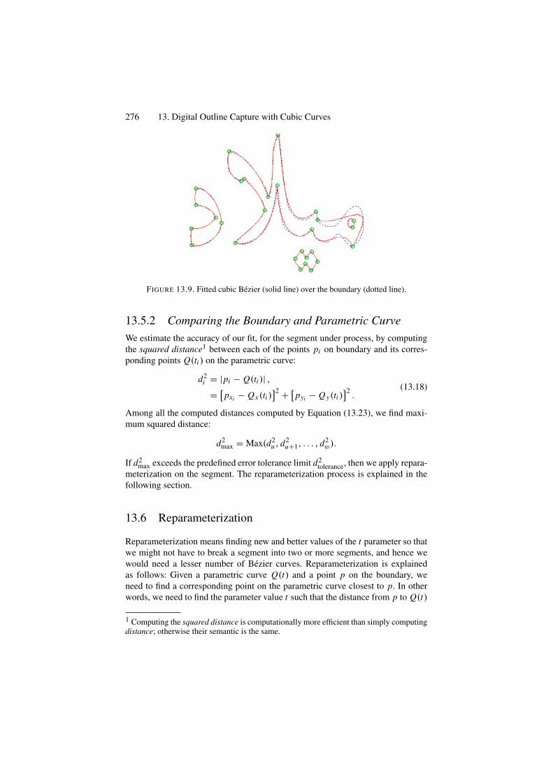
276 13. Digital Outline Capture with Cubic Curves
FIGURE 13.9. Fitted cubic Bezier (solid line) over the boundary (dotted line).
13.5.2 Comparing the Boundary and Parametric CurveWe estimate the accuracy of our fit, for the segment under process, by computingthe squared distance1 between each of the points pi on boundary and its corres-ponding points Q(ti ) on the parametric curve:
d2i = |pi − Q(ti )| ,
= [pxi − Qx (ti )]2 + [pyi − Qy(ti )
]2.
(13.18)
Among all the computed distances computed by Equation (13.23), we find maxi-mum squared distance:
d2max = Max(d2
u , d2u+1, . . . , d2
w).
If d2max exceeds the predefined error tolerance limit d2
tolerance, then we apply repara-meterization on the segment. The reparameterization process is explained in thefollowing section.
13.6 Reparameterization
Reparameterization means finding new and better values of the t parameter so thatwe might not have to break a segment into two or more segments, and hence wewould need a lesser number of Bezier curves. Reparameterization is explainedas follows: Given a parametric curve Q(t) and a point p on the boundary, weneed to find a corresponding point on the parametric curve closest to p. In otherwords, we need to find the parameter value t such that the distance from p to Q(t)
1 Computing the squared distance is computationally more efficient than simply computingdistance; otherwise their semantic is the same.
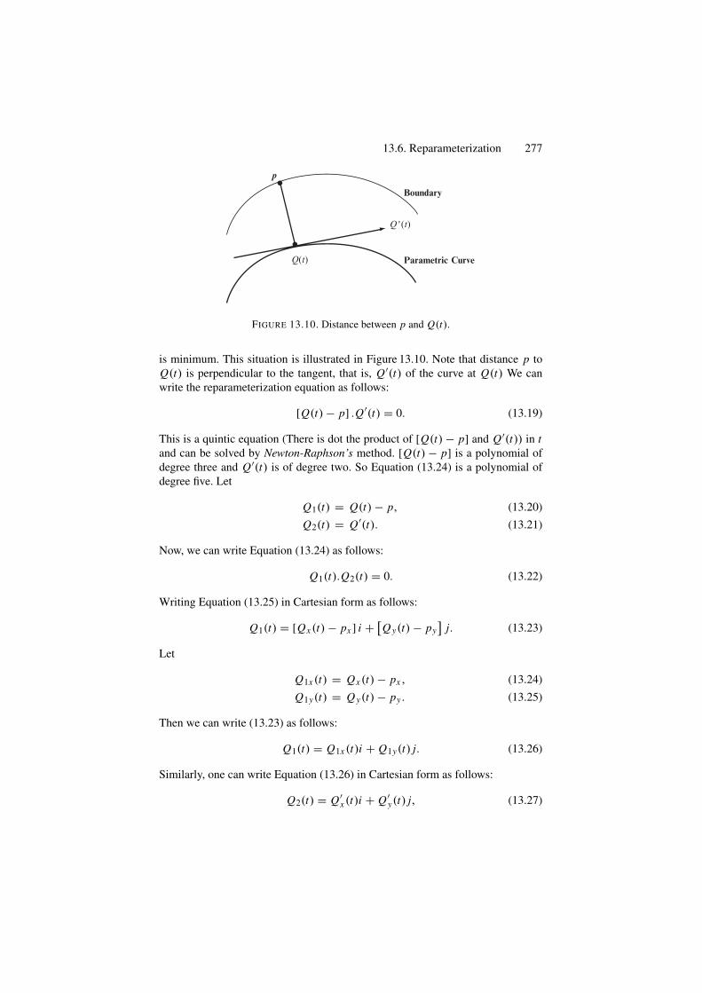
13.6. Reparameterization 277
Q(t)
p
Q ' (t)
Boundary
Parametric Curve
FIGURE 13.10. Distance between p and Q(t).
is minimum. This situation is illustrated in Figure 13.10. Note that distance p toQ(t) is perpendicular to the tangent, that is, Q′(t) of the curve at Q(t) We canwrite the reparameterization equation as follows:
[Q(t) − p] .Q′(t) = 0. (13.19)
This is a quintic equation (There is dot the product of [Q(t) − p] and Q′(t)) in tand can be solved by Newton-Raphson’s method. [Q(t) − p] is a polynomial ofdegree three and Q′(t) is of degree two. So Equation (13.24) is a polynomial ofdegree five. Let
Q1(t) = Q(t) − p, (13.20)Q2(t) = Q′(t). (13.21)
Now, we can write Equation (13.24) as follows:
Q1(t).Q2(t) = 0. (13.22)
Writing Equation (13.25) in Cartesian form as follows:
Q1(t) = [Qx (t) − px ] i + [Qy(t) − py]
j. (13.23)
Let
Q1x (t) = Qx (t) − px , (13.24)Q1y(t) = Qy(t) − py . (13.25)
Then we can write (13.23) as follows:
Q1(t) = Q1x (t)i + Q1y(t) j. (13.26)
Similarly, one can write Equation (13.26) in Cartesian form as follows:
Q2(t) = Q′x (t)i + Q′
y(t) j, (13.27)
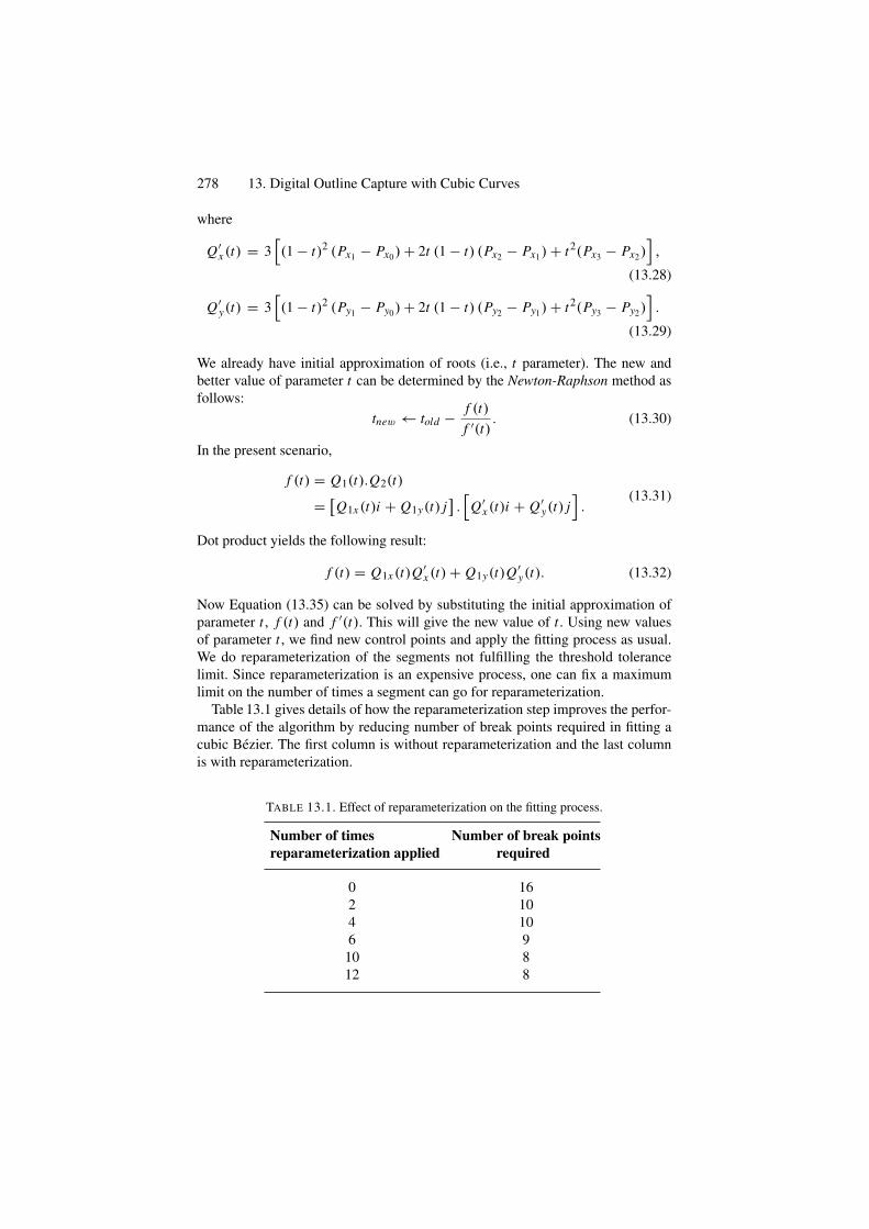
278 13. Digital Outline Capture with Cubic Curves
where
Q′x (t) = 3
[(1 − t)2 (Px1 − Px0) + 2t (1 − t) (Px2 − Px1) + t2(Px3 − Px2)
],
(13.28)
Q′y(t) = 3
[(1 − t)2 (Py1 − Py0) + 2t (1 − t) (Py2 − Py1) + t2(Py3 − Py2)
].
(13.29)
We already have initial approximation of roots (i.e., t parameter). The new andbetter value of parameter t can be determined by the Newton-Raphson method asfollows:
tnew ← told − f (t)f ′(t)
. (13.30)
In the present scenario,
f (t) = Q1(t).Q2(t)
= [Q1x (t)i + Q1y(t) j].[
Q′x (t)i + Q′
y(t) j].
(13.31)
Dot product yields the following result:
f (t) = Q1x (t)Q′x (t) + Q1y(t)Q′
y(t). (13.32)
Now Equation (13.35) can be solved by substituting the initial approximation ofparameter t , f (t) and f ′(t). This will give the new value of t . Using new valuesof parameter t , we find new control points and apply the fitting process as usual.We do reparameterization of the segments not fulfilling the threshold tolerancelimit. Since reparameterization is an expensive process, one can fix a maximumlimit on the number of times a segment can go for reparameterization.
Table 13.1 gives details of how the reparameterization step improves the perfor-mance of the algorithm by reducing number of break points required in fitting acubic Bezier. The first column is without reparameterization and the last columnis with reparameterization.
TABLE 13.1. Effect of reparameterization on the fitting process.
Number of times Number of break pointsreparameterization applied required
0 162 104 106 910 812 8
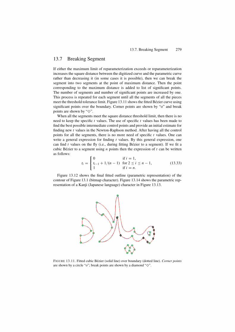
13.7. Breaking Segment 279
13.7 Breaking Segment
If either the maximum limit of reparameterization exceeds or reparameterizationincreases the square distance between the digitized curve and the parametric curverather than decreasing it (in some cases it is possible), then we can break thesegment into two segments at the point of maximum distance. Then the pointcorresponding to the maximum distance is added to list of significant points.The number of segments and number of significant points are increased by one.This process is repeated for each segment until all the segments of all the piecesmeet the threshold tolerance limit. Figure 13.11 shows the fitted Bezier curve usingsignificant points over the boundary. Corner points are shown by “o” and breakpoints are shown by “♦”.
When all the segments meet the square distance threshold limit, then there is noneed to keep the specific t values. The use of specific t values has been made tofind the best possible intermediate control points and provide an initial estimate forfinding new t values in the Newton-Raphson method. After having all the controlpoints for all the segments, there is no more need of specific t values. One canwrite a general expression for finding t values. By this general expression, onecan find t values on the fly (i.e., during fitting Bezier to a segment). If we fit acubic Bezier to a segment using n points then the expression of t can be writtenas follows:
ti =⎧⎨
⎩
0 if i = 1,ti−1 + 1/(n − 1) for 2 ≤ i ≤ n − 1,1 if i = n.
(13.33)
Figure 13.12 shows the final fitted outline (parametric representation) of thecontour of Figure 13.1 (bitmap character). Figure 13.14 shows the parametric rep-resentation of a Kanji (Japanese language) character in Figure 13.13.
FIGURE 13.11. Fitted cubic Bezier (solid line) over boundary (dotted line). Corner pointsare shown by a circle “o”; break points are shown by a diamond “♦”.
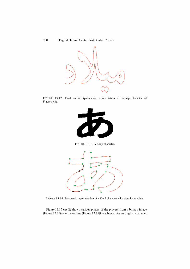
280 13. Digital Outline Capture with Cubic Curves
FIGURE 13.12. Final outline (parametric representation of bitmap character ofFigure 13.1).
FIGURE 13.13. A Kanji character.
FIGURE 13.14. Parametric representation of a Kanji character with significant points.
Figure 13.15 (a)-(f) shows various phases of the process from a bitmap image(Figure 13.15(a) to the outline (Figure 13.15(f)) achieved for an English character
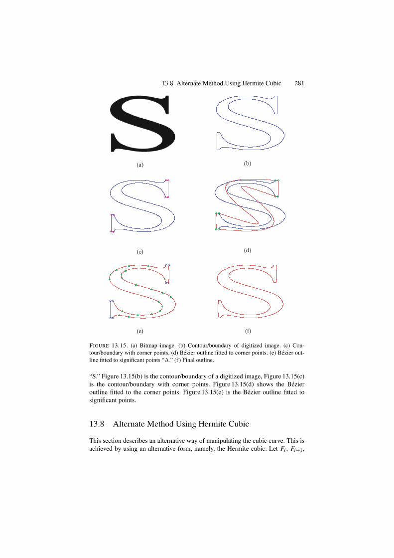
13.8. Alternate Method Using Hermite Cubic 281
(a) (b)
(c) (d)
(e) (f)
FIGURE 13.15. (a) Bitmap image. (b) Contour/boundary of digitized image. (c) Con-tour/boundary with corner points. (d) Bezier outline fitted to corner points. (e) Bezier out-line fitted to significant points “�.” (f ) Final outline.
“S.” Figure 13.15(b) is the contour/boundary of a digitized image, Figure 13.15(c)is the contour/boundary with corner points. Figure 13.15(d) shows the Bezieroutline fitted to the corner points. Figure 13.15(e) is the Bezier outline fitted tosignificant points.
13.8 Alternate Method Using Hermite Cubic
This section describes an alternative way of manipulating the cubic curve. This isachieved by using an alternative form, namely, the Hermite cubic. Let Fi , Fi+1,
282 13. Digital Outline Capture with Cubic Curves
i ∈ Z , be the two end characteristic points given at the distinct knots ti , ti+1, i ∈ Zwith interval spacing hi = ti+1 − ti > 0. Also let Di , Di+1, i ∈ Z denote the firstderivative values defined at the knots. Then the generalized form of the cubic isdefined by:
Pi |(ti ,ti+1)(t) = (1 − t)3 Fi + 3t (1 − t)2Vi + 3t2(1 − t) + t3 Fi+1, (13.34)
whereVi = Fi + hi Di/3, Wi = Fi+1 − hi Di+1/3,
The interpolation conditions, ∀i are as follows:
Pi (ti ) = Fi ,Pi (ti+1) = Fi+1,
P(1)i (ti ) = Di ,
P(1)i (ti+1) = Di+1.
⎫⎪⎪⎬
⎪⎪⎭
Equation (13.34) can be rewritten as
Pi |(ti ,ti+1)(t) = R0,i (t)Fi + R1,i (t)Vi + R2,i (t) + R3,i (t)Fi+1,
whereR0,i (t) = (1 − t)3,
R1,i (t) = 3t (1 − t)2,
R2,i (t) = 3t2(1 − t),R3,i (t) = t3.
⎫⎪⎪⎬
⎪⎪⎭
One can see that the functions R j,i , j = 0, 1, 2, 3 are Bernstein-Bezier basis func-tions, such that
3∑
j=0
R j,i (t) = 1.
One can also observe that the piecewise curve, thus obtained, results to a cubicspline with C1 continuity.
13.8.1 Estimation of Tangent VectorsWe define a distance-based choice for tangent vectors Di ’s at Fi ’s as follows. Foropen curves, the tangents are defined as follows:
D0 = 2 (F1 − F0) − (F2 − F0) /2,Dn = 2 (Fn − Fn−1) − (Fn − Fn−2) /2,Di = ai (Fi − Fi−1) + (1 − ai ) (Fi+1 − Fi ) , i = 1, . . . , n − 1.
⎫⎬
⎭
For close curves, the tangents are described as follows:
F−1 = Fn−1, Fn+1 = F1,Di = ai (Fi − Fi−1) + (1 − ai ) (Fi+1 − Fi ) , i = 0, . . . , n,
}
whereai = |Fi+1 − Fi |
|Fi+1 − Fi | + |Fi − Fi−1| , i = 0, . . . , n.
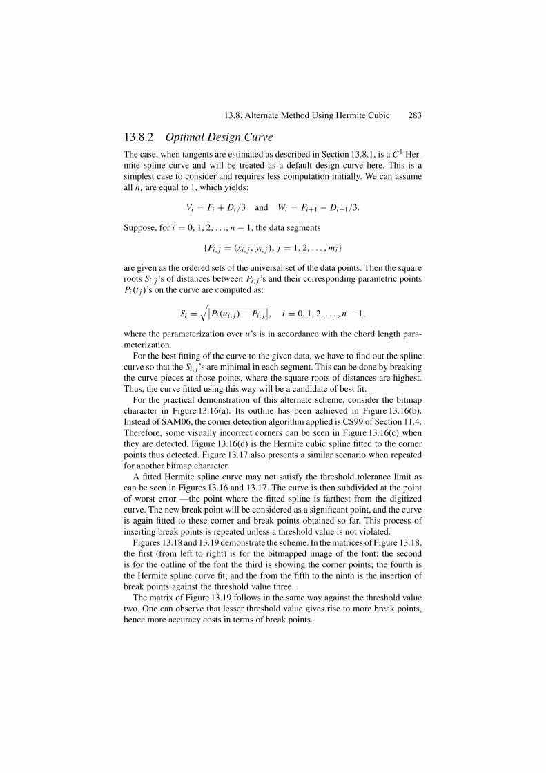
13.8. Alternate Method Using Hermite Cubic 283
13.8.2 Optimal Design CurveThe case, when tangents are estimated as described in Section 13.8.1, is a C1 Her-mite spline curve and will be treated as a default design curve here. This is asimplest case to consider and requires less computation initially. We can assumeall hi are equal to 1, which yields:
Vi = Fi + Di/3 and Wi = Fi+1 − Di+1/3.
Suppose, for i = 0, 1, 2, . . ., n − 1, the data segments
{Pi, j = (xi, j , yi, j ), j = 1, 2, . . . , mi }are given as the ordered sets of the universal set of the data points. Then the squareroots Si, j ’s of distances between Pi, j ’s and their corresponding parametric pointsPi (t j )’s on the curve are computed as:
Si =√∣∣Pi (ui, j ) − Pi, j
∣∣, i = 0, 1, 2, . . . , n − 1,
where the parameterization over u’s is in accordance with the chord length para-meterization.
For the best fitting of the curve to the given data, we have to find out the splinecurve so that the Si, j ’s are minimal in each segment. This can be done by breakingthe curve pieces at those points, where the square roots of distances are highest.Thus, the curve fitted using this way will be a candidate of best fit.
For the practical demonstration of this alternate scheme, consider the bitmapcharacter in Figure 13.16(a). Its outline has been achieved in Figure 13.16(b).Instead of SAM06, the corner detection algorithm applied is CS99 of Section 11.4.Therefore, some visually incorrect corners can be seen in Figure 13.16(c) whenthey are detected. Figure 13.16(d) is the Hermite cubic spline fitted to the cornerpoints thus detected. Figure 13.17 also presents a similar scenario when repeatedfor another bitmap character.
A fitted Hermite spline curve may not satisfy the threshold tolerance limit ascan be seen in Figures 13.16 and 13.17. The curve is then subdivided at the pointof worst error —the point where the fitted spline is farthest from the digitizedcurve. The new break point will be considered as a significant point, and the curveis again fitted to these corner and break points obtained so far. This process ofinserting break points is repeated unless a threshold value is not violated.
Figures 13.18 and 13.19 demonstrate the scheme. In the matrices of Figure 13.18,the first (from left to right) is for the bitmapped image of the font; the secondis for the outline of the font the third is showing the corner points; the fourth isthe Hermite spline curve fit; and the from the fifth to the ninth is the insertion ofbreak points against the threshold value three.
The matrix of Figure 13.19 follows in the same way against the threshold valuetwo. One can observe that lesser threshold value gives rise to more break points,hence more accuracy costs in terms of break points.
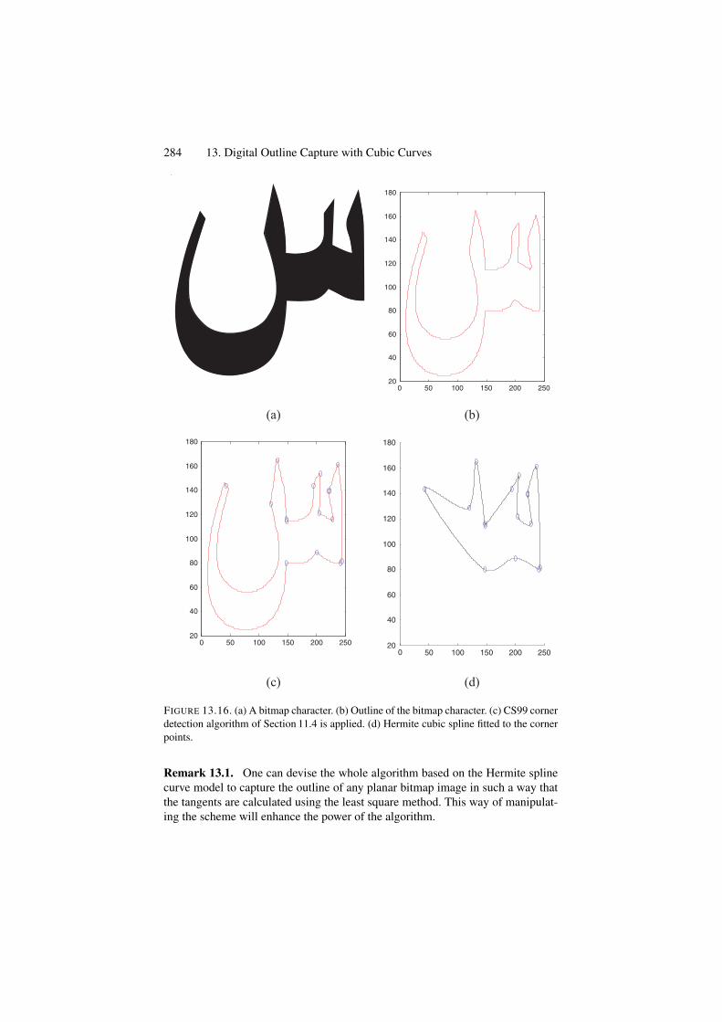
284 13. Digital Outline Capture with Cubic Curves
0 50 100 150 200 25020
40
60
80
100
120
140
160
180
0 50 100 150 200 25020
40
60
80
100
120
140
160
180
0 50 100 150 200 25020
40
60
80
100
120
140
160
180
(c) (d)
(a) (b)
FIGURE 13.16. (a) A bitmap character. (b) Outline of the bitmap character. (c) CS99 cornerdetection algorithm of Section 11.4 is applied. (d) Hermite cubic spline fitted to the cornerpoints.
Remark 13.1. One can devise the whole algorithm based on the Hermite splinecurve model to capture the outline of any planar bitmap image in such a way thatthe tangents are calculated using the least square method. This way of manipulat-ing the scheme will enhance the power of the algorithm.
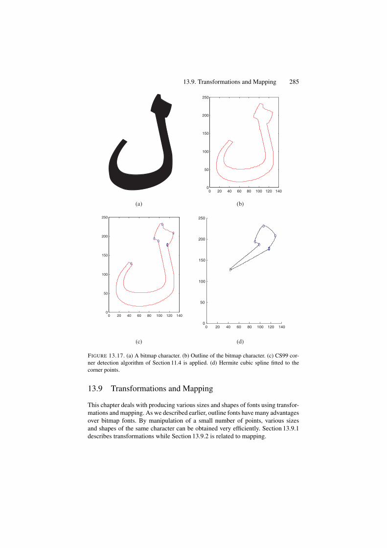
13.9. Transformations and Mapping 285
0 20 40 60 80 100 120 1400
50
100
150
200
250
(a) (b)
(c) (d)
0 20 40 60 80 100 120 1400
50
100
150
200
250
0 20 40 60 80 100 120 1400
50
100
150
200
250
FIGURE 13.17. (a) A bitmap character. (b) Outline of the bitmap character. (c) CS99 cor-ner detection algorithm of Section 11.4 is applied. (d) Hermite cubic spline fitted to thecorner points.
13.9 Transformations and Mapping
This chapter deals with producing various sizes and shapes of fonts using transfor-mations and mapping. As we described earlier, outline fonts have many advantagesover bitmap fonts. By manipulation of a small number of points, various sizesand shapes of the same character can be obtained very efficiently. Section 13.9.1describes transformations while Section 13.9.2 is related to mapping.
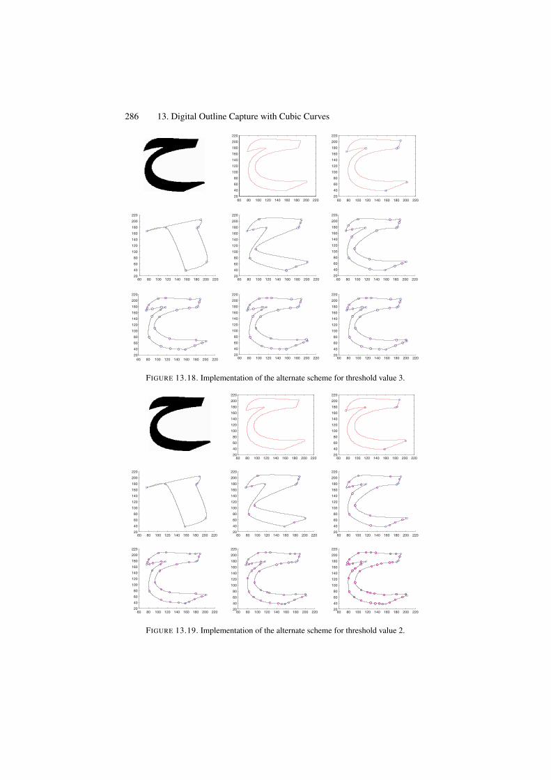
286 13. Digital Outline Capture with Cubic Curves
60 80 100 120 140 160 180 200 22020
40
60
80
100
120
140
160
180
200
220
60 80 100 120 140 160 180 200 22020
40
60
80
100
120
140
160
180
200
220
60 80 100 120 140 160 180 200 22020
40
60
80
100
120
140
160
180
200
220
60 80 100 120 140 160 180 200 22020
40
60
80
100
120
140
160
180
200
220
60 80 100 120 140 160 180 200 22020
40
60
80
100
120
140
160
180
200
220
60 80 100 120 140 160 180 200 22020
40
60
80
100
120
140
160
180
200
220
60 80 100 120 140 160 180 200 22020
40
60
80
100
120
140
160
180
200
220
60 80 100 120 140 160 180 200 22020
40
60
80
100
120
140
160
180
200
220
FIGURE 13.18. Implementation of the alternate scheme for threshold value 3.
60 80 100 120 140 160 180 200 22020
40
60
80
100
120
140
160
180
200
220
60 80 100 120 140 160 180 200 22020
40
60
80
100
120
140
160
180
200
220
60 80 100 120 140 160 180 200 22020
40
60
80
100
120
140
160
180
200
220
60 80 100 120 140 160 180 200 22020
40
60
80
100
120
140
160
180
200
220
60 80 100 120 140 160 180 200 22020
40
60
80
100
120
140
160
180
200
220
60 80 100 120 140 160 180 200 22020
40
60
80
100
120
140
160
180
200
220
60 80 100 120 140 160 180 200 22020
40
60
80
100
120
140
160
180
200
220
60 80 100 120 140 160 180 200 22020
40
60
80
100
120
140
160
180
200
220
FIGURE 13.19. Implementation of the alternate scheme for threshold value 2.
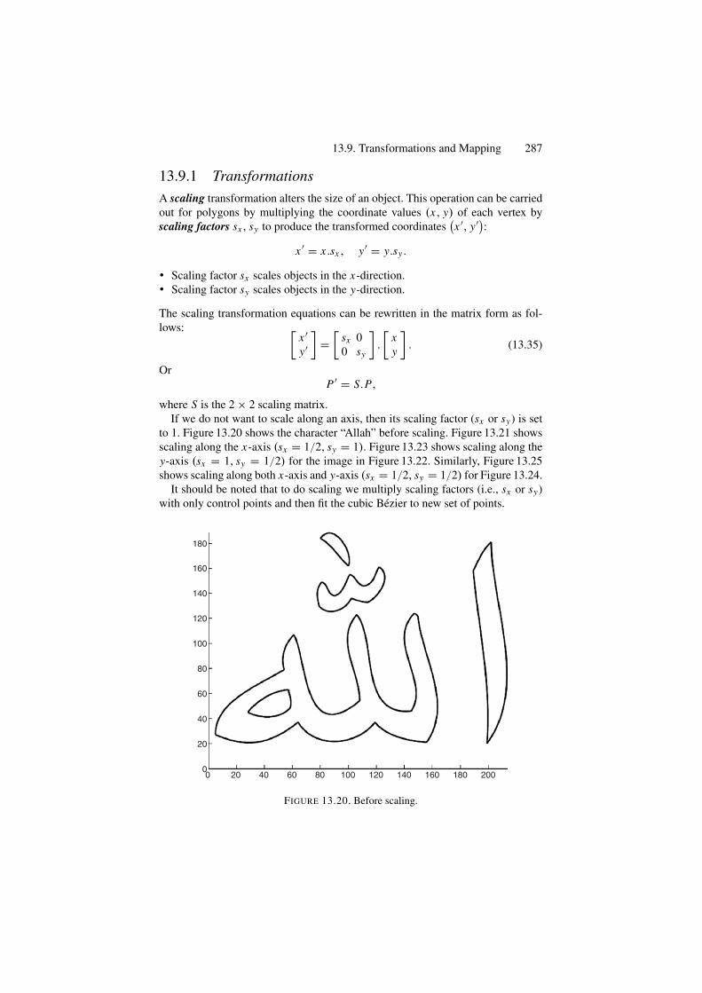
13.9. Transformations and Mapping 287
13.9.1 TransformationsA scaling transformation alters the size of an object. This operation can be carriedout for polygons by multiplying the coordinate values (x, y) of each vertex byscaling factors sx , sy to produce the transformed coordinates
(x ′, y′):
x ′ = x .sx , y′ = y.sy .
• Scaling factor sx scales objects in the x-direction.• Scaling factor sy scales objects in the y-direction.
The scaling transformation equations can be rewritten in the matrix form as fol-lows: [
x ′y′]
=[
sx 00 sy
].
[xy
]. (13.35)
OrP ′ = S.P,
where S is the 2 × 2 scaling matrix.If we do not want to scale along an axis, then its scaling factor (sx or sy) is set
to 1. Figure 13.20 shows the character “Allah” before scaling. Figure 13.21 showsscaling along the x-axis (sx = 1/2, sy = 1). Figure 13.23 shows scaling along they-axis (sx = 1, sy = 1/2) for the image in Figure 13.22. Similarly, Figure 13.25shows scaling along both x-axis and y-axis (sx = 1/2, sy = 1/2) for Figure 13.24.
It should be noted that to do scaling we multiply scaling factors (i.e., sx or sy)with only control points and then fit the cubic Bezier to new set of points.
180
160
140
120
100
80
60
40
20
00 20 40 60 80 100 120 140 160 180 200
FIGURE 13.20. Before scaling.
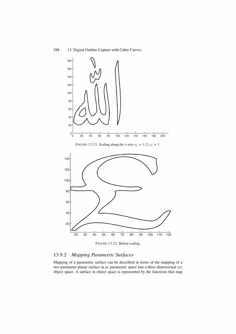
288 13. Digital Outline Capture with Cubic Curves
180
140
120
100
60
40
00 20 40 60 80 100 120 140 160 180 200
20
80
160
FIGURE 13.21. Scaling along the x-axis sx = 1/2; sy = 1.
140
120
100
80
60
40
20
20 30 40 50 60 70 80 90 100 110 120
FIGURE 13.22. Before scaling.
13.9.2 Mapping Parametric SurfacesMapping of a parametric surface can be described in terms of the mapping of atwo-parameter planar surface in uv parametric space into a three-dimensional xyzobject space. A surface in object space is represented by the functions that map
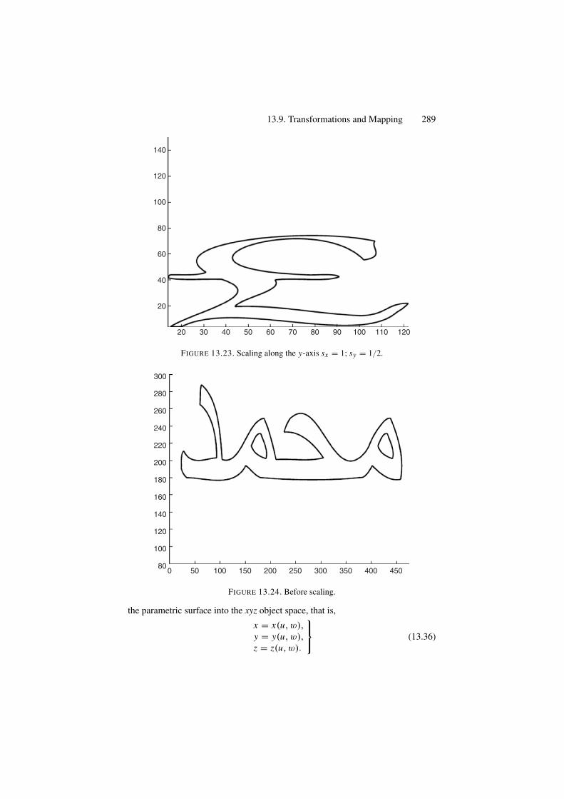
13.9. Transformations and Mapping 289
140
120
100
80
60
40
20
20 30 40 50 60 70 80 90 100 110 120
FIGURE 13.23. Scaling along the y-axis sx = 1; sy = 1/2.
300
280
260
240
220
200
180
160
140
120
100
800 50 100 150 200 250 300 350 400 450
FIGURE 13.24. Before scaling.
the parametric surface into the xyz object space, that is,
x = x(u, w),y = y(u, w),z = z(u, w).
⎫⎬
⎭(13.36)
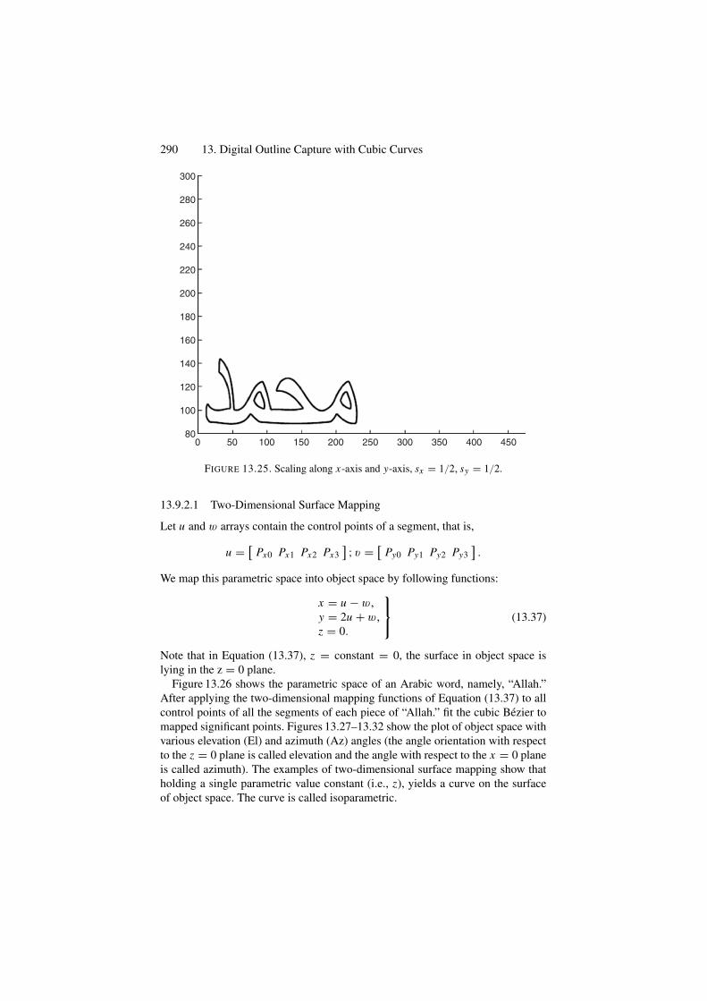
290 13. Digital Outline Capture with Cubic Curves
300
280
260
240
220
200
180
160
140
120
100
800 50 100 150 200 250 300 350 400 450
FIGURE 13.25. Scaling along x-axis and y-axis, sx = 1/2, sy = 1/2.
13.9.2.1 Two-Dimensional Surface Mapping
Let u and w arrays contain the control points of a segment, that is,
u = [ Px0 Px1 Px2 Px3] ; v = [ Py0 Py1 Py2 Py3
].
We map this parametric space into object space by following functions:
x = u − w,y = 2u + w,z = 0.
⎫⎬
⎭(13.37)
Note that in Equation (13.37), z = constant = 0, the surface in object space islying in the z = 0 plane.
Figure 13.26 shows the parametric space of an Arabic word, namely, “Allah.”After applying the two-dimensional mapping functions of Equation (13.37) to allcontrol points of all the segments of each piece of “Allah.” fit the cubic Bezier tomapped significant points. Figures 13.27–13.32 show the plot of object space withvarious elevation (El) and azimuth (Az) angles (the angle orientation with respectto the z = 0 plane is called elevation and the angle with respect to the x = 0 planeis called azimuth). The examples of two-dimensional surface mapping show thatholding a single parametric value constant (i.e., z), yields a curve on the surfaceof object space. The curve is called isoparametric.

13.9. Transformations and Mapping 291
FIGURE 13.26. Parametric space.
FIGURE 13.27. 2-D Surface mapping. Object space. Az = 30◦, El = 30◦.
FIGURE 13.28. 2-D Surface mapping. Object space. Az = 45◦, El = 45◦.
FIGURE 13.29. 2-D Surface mapping. Object space. Az = 160◦, El = 160◦.
FIGURE 13.30. 2-D surface mapping. Object space. Az = 210◦, El = 210◦.
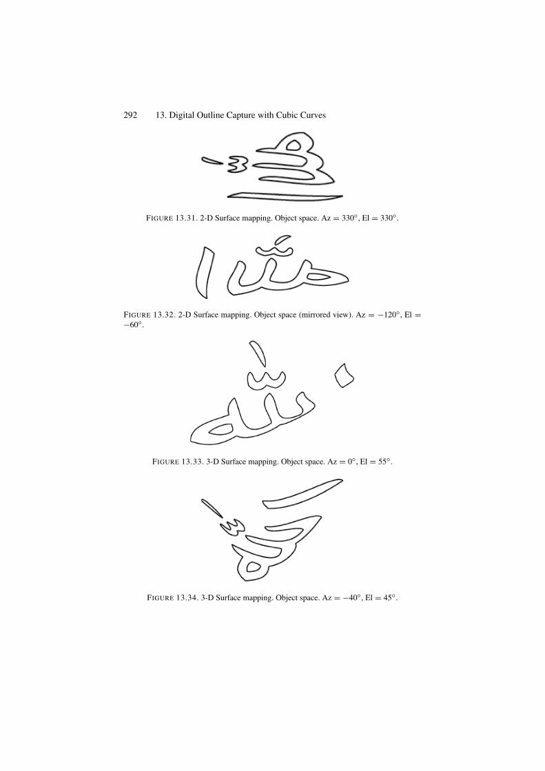
292 13. Digital Outline Capture with Cubic Curves
FIGURE 13.31. 2-D Surface mapping. Object space. Az = 330◦, El = 330◦.
FIGURE 13.32. 2-D Surface mapping. Object space (mirrored view). Az = −120◦, El =−60◦.
FIGURE 13.33. 3-D Surface mapping. Object space. Az = 0◦, El = 55◦.
FIGURE 13.34. 3-D Surface mapping. Object space. Az = −40◦, El = 45◦.
13.11. Exercises 293
13.9.2.2 Three-Dimensional Surface Mapping
Similarly, as in the previous section, one can apply three-dimensional mapping tomap parametric space into object space. In this case, mapping functions may bethe following:
x = u,y = w,
z = (u − w)2 .
⎫⎬
⎭(13.38)
This selection of mapping functions is based on following criteria:
• The legibility of the character should be preserved.• A continuous segment must not map to a discontinuous segment.
13.10 Summary
We have presented an efficient algorithm for approximation of the boundary ofdigital character images. The algorithm is particularly suitable for languages thatare highly curvilinear in nature, such as Arabic, Japanese, Urdu, and so on. Inaddition to the detection of corner points, a strategy to detect a set of break pointshas also also been explained to optimize the outline. Parametric cubic Beziercurves are used for fitting. Filtering noise and reparameterization steps are addedto improve the performance of the algorithm. The proposed approach eliminatesthe human interaction in obtaining the outline of the original character [18].
13.11 Exercises
1. Using a Gaussian filter, write a program to filter the outlines of images.2. Repeat the filtering process in Exercise 1 a number of times and explain the
difference you observe.3. Repeat the filtering process in Exercise 1 a number of times and explain the
difference you observe when
a. the corner points are included,b. the corner points are excluded.
4. Write a program to detect corner points using the SAM06 corner detectionalgorithm and then filter the noise in such a way that the corner points remainincluded. Do you think the claim in the book is justified, that, due to this strat-egy, corner points are detected more accurately and the overall shape of char-acter is more intact?
5. Write a program using chord length parameterization to plot a Bezier cubiccurve with given four input control points.
6. Write a program using unit length parameterization to plot a Bezier cubic curvewith given four input control points.
294 13. Digital Outline Capture with Cubic Curves
7. How different would the two Bezier cubic curves, in Exercises 5 and 6, lookwhen fitted to the following control points:
a. P0 = (0, 0) , P1 = (5, 10) , P2 = (15, 15) , P3 = (25, 5) ,b. P0 = (0, 0) , P1 = (5, 10) , P2 = (−10, 15) , P3 = (5, 5) ,c. P0 = (0, 0) , P1 = (5, 10) , P2 = (15,−15) , P3 = (25, 5) ,d. P0 = (0, 0) , P1 = (5, 10) , P2 = (15, 15) , P3 = (0, 0) .
8. Find the intermediate control points for the following data (read from left toright in order) when a Bezier cubic is fitted as in Section 13.4.1:
a. (0, 0), (5, 10), (15, 15), (25, 5), (30, 20), (30, 30), (35, 40),b. (0, 0), (1, 10), (2, 11), (3, 12), (4, 13), (5, 15), (6, 17), (7, 17),
9. Write a program using chord length parameterization to plot a Hermite cubiccurve with given input data points as given in Exercises 7 and 8.
10. Write a program using unit length parameterization to plot a Hermite cubiccurve with given input data points as in Exercises 7 and 8.
11. Write a program to implement the whole algorithm based on the Bezier curvemodel to capture the outline of any planar bitmap image.
12. How different would the two Hermite cubic curves in Exercises 10 and 11 lookwhen fitted?
13. Write a program to implement the whole algorithm based on the Hermitespline curve model to capture the outline of any planar bitmap image.
14. Devise the whole algorithm based on the Hermite spline curve model to cap-ture the outline of any planar bitmap image in such a way that the tangents arecalculated using the least square method.
References1. Karow, P. (1994), Digital Typefaces: Description and Formats. Springer-Verlag,
Berlin.2. Karow, P. (1994), Font Technology: Methods and Tools. Springer-Verlag, Berlin.3. Beus, H.L. (1987), An improved corner detection algorithm based on chain-coded
plane curves. Pattern Recognition 20(3):291–296.4. Liu, H.C., and Srinath, M.D. (1990), Corner detection from chain-code. Pattern Recog-
nition, 51–68.5. Sarfraz, M., and Khan, M.A. (2003), An automatic outline-fitting algorithm for Arabic
characters. Lecture Notes in Computer Sciences (LNCS) 2669, 589–598\.6. Sarfraz, M., and Khan. M.A. (2002), Automatic outline capture of Arabic fonts. Infor-
mation Sciences, 269–281.7. Avrahami, G., and Pratt, V. (1991), Subpixel edge detection in character digitization.
Raster Imaging and Digital Typography II, 54–64.8. Hou. Z.J., and Wei, G.W. (2002), A new approach to edge detection, Pattern Recogni-
tion 35, 1559–1570.9. Richard, N., and Gilbert, T. (2002), Extraction of dominant points by estimation of the
contour fluctuations, Pattern Recognition (35), 1447–1462.

References 295
10. Pei, S. (1994), Corner detection using nest moving average. Pattern Recognition,27(11):1533–1537.
11. Chetrikov, D., and Zsabo, S. (1999), A simple and efficient algorithm for detection ofhigh curvature points in planar curves, Proc. 23rd Workshop of the Australian PatternRecognition Group, 1751–184.
12. Davis, L. (1979), Shape matching using relaxation techniques. IEEE Trans. PAMI.60–72.
13. Braquelaire, J.P., and Vialard, A. (1997), A new anti-aliasing approach for image com-positing. The Visual Computer, 13(5), 218–227.
14. Fabris, A.E., and A.R. Forrest. (1997), Anti-aliasing of curves by discrete prefiltering.SIGGRAPH 1997 Proceedings, pp. 317–326.
15. Cox, M.G. (1971), Curve fitting with piecewise polynomials. J. Inst. Math Appl. 8,36–52.
16. Plass, M., and Stone, M. (1983), Curve-fitting with piecewise parametric cubics. Com-puter Graphics 17(3), 229–239.
17. Zhang, S., Li, L., Seah, H.S. (1998), Recursive curve fitting and rendering. The VisualComputer, 69–82.
18. Sarfraz, M., and Khan, M.A. (2004), An automatic algorithm for approximatingboundary of bitmap characters. In: Future Generation Computer Systems, ElsevierScience, Vol. 20, pp. 1327–1336.
19. Sarfraz, M. (2004), Some algorithms for curve design and automatic outline capturingof images, Int J Image Graphics, World Scientific Publisher, 4(2), 301–324.
20. Sarfraz, M. (2003), Curve fitting for large data using rational cubic splines, Int J Com-put Their Appl 10(4), 233–246.
21. Sarfraz, M., and Khan, M.A. (2003), An automatic outline fitting algorithm for Ara-bic characters, Lecture Notes in Computer Science, Vol. 2669: Computational Scienceand Its Applications, Eds.: V. Kumar, M.L. Gavrilova, C.J.K. Tan, and P.L’Ecuyer,Springer-Verlag, New York, pp. 589–598.
22. Sarfraz, M. (2003), Optimal curve fitting to digital data, Int J WSCG 11(1), 128–135.23. Sarfraz, M., and Razzak, M.F.A. (2003), A web-based system to capture outlines of
Arabic fonts, Int J Infor Sci. Elsevier Science, 150(3–4), 177–193.24. Sarfraz, M., and Razzak, M.F.A. (2002), An algorithm for automatic capturing of font
outlines, Int J Comput Graphics, Elsevier Science, 26(5), 795–804.25. Sarfraz, M., and Khan, M.A. (2002), Automatic outline capture of Arabic fonts, Int J
Infor Sci, Elsevier Science, 140(3–4), 269–281.26. Sarfraz, M., Riyazuddin, M. and Baig, M.H. (2006), Capturing planar shapes by
approximating their outlines, Int J Computational Appl Math, Elsevier Science, 189(1–2), 494–512.
27. Sarfraz, M. (2004), Representing shapes by fitting data using an evolutionaryapproach, Int J Comput Aided Design Appl 1(1–4), 179–186.
28. Sarfraz, M., and Raza, A. (2002), Towards automatic recognition of fonts using geneticapproach, Recent Advances in Computers, Computing, and Communications, Eds.:N. Mastorakis and V. Mladenov, WSEAS Press, 290–295.
29. Sarfraz, M. (2003), Outline representation of fonts using genetic approach, Advancesin Soft Computing: Engineering Design and Manufacturing, Eds.: Benitez, J.M.,Cordon, O., Hoffmann, F., and Roy, R., Springer-Verlag, New York, pp. 109–118.
14Computer-Aided Reverse EngineeringUsing Evolutionary Heuristicson NURBS
Abstract. This chapter is related to the issue of computer-aided reverse engineering.Although the proposed techniques have been presented for image-based planar objects, itis extendable to the objects in 3D with some modifications. Two nondeterministic evolution-ary approaches have been presented. Nonuniform rational B-splines (NURBS) have beenutilized as an underlying approximation curve scheme. Simulated annealing and simulatedevolution heuristics are used as evolutionary methodologies. The optimized NURBS modelshave been fitted over the contour data of the planar shapes for the ultimate and automaticoutput. The output results are visually pleasing with respect to the threshold provided bythe user.
14.1 Introduction
Computer-aided reverse engineering (CARE) is an important area of study inthe modern age of computers. Many solutions in modern industry are providedfor design and manufacturing [12–16, 19]. In modern design, scanned digitaldata leads to using contour styling [9, 10] which helps to guide visual accep-tance after adopting some curve or surface approximation scheme [3, 5, 7]. Var-ious objects including manufactured parts or human body parts are designedand redesigned with complex free-form geometry. This trend can be foundin recent years in various applications such as vehicle body design. The wideacceptance of free-form curves and surfaces for component design can also beattributed to advances in curve and surface modelling and their implementationsin CAD/CAM/CAE/CARE systems.
Although the techniques of using curve and surface models for representingcomplex geometries have become quite mature and stable, people still debateusing an appropriate model for a specific application. From the perspective ofreverse engineering, nonuniform rational B-spline (NURBS) curves and surfacescan approximate complex geometry more accurately and effectively. However,
297
298 14 Computer-Aided Reverse Engineering
curve or surface approximation using NURBS has not been found in many practi-cal applications in recent years. One of the reasons is that methods for computingthe best rational approximation are in general nonlinear [17]. With large amountsof digitized data and heavy computations in the case of multivariable nonlinearequations, the amount of computation time is too expensive and is almost notaffordable in most of the CARE practices. This is one of the reasons that mostof the designers frequently use a B-spline curve or surface approximation. Butit is a fact that the accuracy requirement in curve and surface approximation iscontinuously increasing due to very complex models being faced in the industry.
Although increasing the number of control points of B-splines can, in gen-eral, improve the curve or surface-fitting accuracy, it is basically against the datareduction principle and will increase the burden of the database [15]. Thus, underthe circumstances when the factors of accuracy and model size are important,the NURBS curve and surface approximation can prove to be a useful solution.However, efficient fitting algorithms are required to be developed and used forNURBS applications.
This study is related to the NURBS curve and surface approximation usingefficient fitting algorithms. In shape design problems, the main objective is toachieve an optimized curve or surface with the least possible computation cost.For complicated shapes with large measurement data, the problem depends onthe selection of appropriate parameters in the description of the curve or surfacemodel. Algorithms based on heuristic techniques such as genetic algorithms (GA),simulated annealing (SimE), simulated evolution (SimE), and so on, can provideus with an approach to finding optimal parameters with reasonable cost. Sincethe data in such problems cannot be approximated with a single polynomial, theapplication of splines, Bezier curves, and so on, are utilized. NURBS [4], whichprovide more local control on the shape of the curve, give a better approximationof the underlying data in shape design problems.
When using NURBS for curve and surface approximation of digitized data, itcan be shown [18] that in the context of optimization the objective function tobe set up is the sum of the squared errors. Since the NURBS consist of multipa-rameters, knots, control points, and weights, the rational format of the objectivefunction makes the fitting task a multivariable nonlinear optimization problem.Although there exist various algorithms for nonlinear optimization problems, theyare typically computationally expensive and time-consuming. Furthermore, whenfaced with a problem that involves many variables, the initial values become verydifficult to predict. This chapter concentrates only on weight parameters to beoptimized so that an optimal curve or surface model can be achieved efficiently.
Since SimE and SimA are heuristics, the problem of initial values will alsobe resolved by assuming their random values. Thus, the optimization problem inthis chapter becomes a univariate optimization problem, which is easy to man-age. This problem was solved in [12,13,19] and is different from other techniquesin [9, 10, 12, 14]. In [9], knots corresponding to the control points have been opti-mized using a genetic algorithm. An approach based on a Tabu search has beenapplied in [14]. An algorithm proposed in [12] discusses optimization of knots
14.2. Preprocessing 299
and weights using simulated annealing. In [10], a novel approach was proposedfor optimization of NURBS control points using SimE. The main objective ofthis chapter is to describe curve or surface-fitting algorithms based on SimE usingNURBS. Here, the shape parameters in the description of the NURBS have beenselected to be computed such that the computed curve or surface provides a best fitto the original data raised from the geometric models after the scanning process.
The chapter is divided into various sections. The following section deals withpreprocessing issues such as image contour extraction and detection of cor-ner points. Section 14.3 gives a brief description of NURBS whereas the SimEalgorithm is discussed in Section 14.4. The approach, with details of the evolu-tionary optimization curve technique, SimE, is described and demonstrated inSection 14.5. The two approaches are demonstrated for surfaces in Section 14.6.The chapter is summarized in Section 14.7.
14.2 Preprocessing
This section is devoted to preprocessing issues such as image contour extractionand detection of corner points.
14.2.1 Image Contour ExtractionA digitized image is obtained from an electronic device or by scanning. For theplanar objects, the quality of a digitized scanned image depends on various factorssuch as the image on paper, scanner type and the attributes set during scanning.The contour of the digitized image is extracted using the boundary detectionalgorithms. There are numerous algorithms for detecting the boundary. In thisstudy, the algorithm used is one proposed by Quddus [8]. The input to this algo-rithm is a bitmap file and the output is the number of boundary points and theirvalues. The algorithm returns a number of boundary points and their values. Asa demonstration, one can see the output in Figures 14.1(b) for the BMP image inFigures 14.1(a). It should be noted that, to acquire 3D data from 3D models, somesophisticated 3D scanners can be used with an appropriate technique.
14.2.2 Detection of Corner PointsDetection of corner points is the next step after finding out contours. The cornerpoints are those points that partition the outline into various segments. A num-ber of approaches have been proposed by researchers; the reader is referred toChapter 11 for details. In this chapter, two different corner detectors, namely CS99(see Section 11.4) and SAM06 (see Section 11.5), have been used. The reverseengineering technique based on the SimE approach in Section 4.4 uses CS99,whereas SAM06 is used for the technique based on SimA in Section 14.5.
Detection of corner points using CS99 with different settings of parameters ismade for Figure 14.1(b). Figure 14.2(a) demonstrates the corner points detected
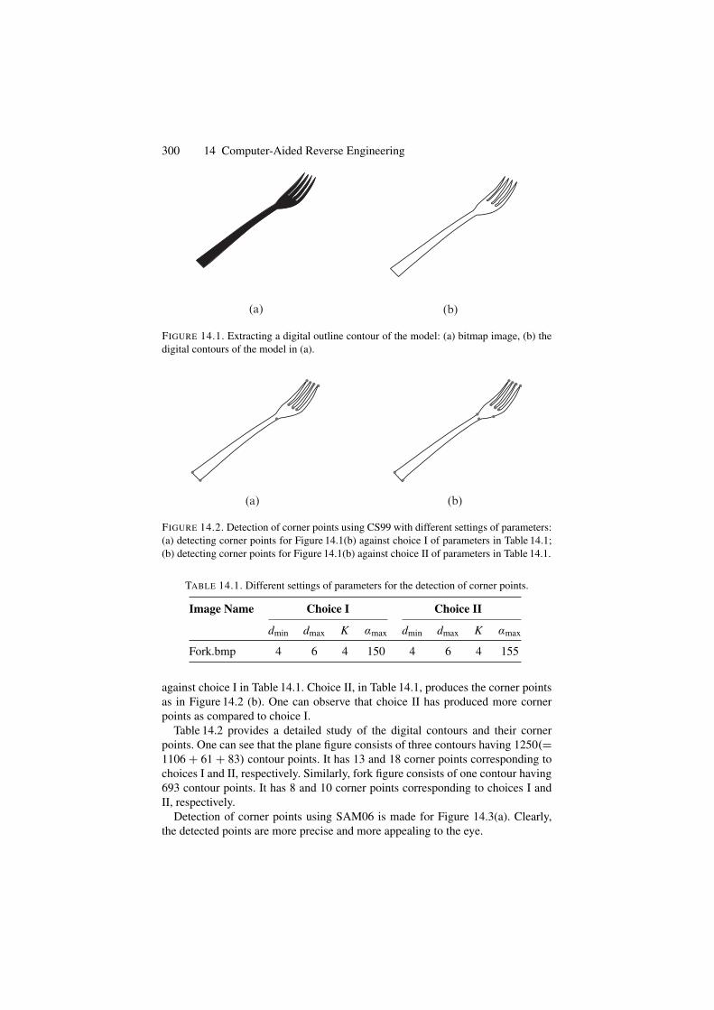
300 14 Computer-Aided Reverse Engineering
(a) (b)
FIGURE 14.1. Extracting a digital outline contour of the model: (a) bitmap image, (b) thedigital contours of the model in (a).
(a) (b)
FIGURE 14.2. Detection of corner points using CS99 with different settings of parameters:(a) detecting corner points for Figure 14.1(b) against choice I of parameters in Table 14.1;(b) detecting corner points for Figure 14.1(b) against choice II of parameters in Table 14.1.
TABLE 14.1. Different settings of parameters for the detection of corner points.
Image Name Choice I Choice II
dmin dmax K αmax dmin dmax K αmax
Fork.bmp 4 6 4 150 4 6 4 155
against choice I in Table 14.1. Choice II, in Table 14.1, produces the corner pointsas in Figure 14.2 (b). One can observe that choice II has produced more cornerpoints as compared to choice I.
Table 14.2 provides a detailed study of the digital contours and their cornerpoints. One can see that the plane figure consists of three contours having 1250(=1106 + 61 + 83) contour points. It has 13 and 18 corner points corresponding tochoices I and II, respectively. Similarly, fork figure consists of one contour having693 contour points. It has 8 and 10 corner points corresponding to choices I andII, respectively.
Detection of corner points using SAM06 is made for Figure 14.3(a). Clearly,the detected points are more precise and more appealing to the eye.
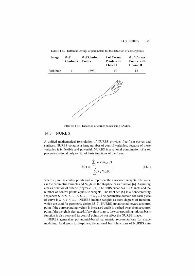
14.3. NURBS 301
TABLE 14.2. Different settings of parameters for the detection of corner points.
Image # ofContours
# of ContourPoints
# of CornerPoints withChoice I
# of CornerPoints withChoice II
Fork.bmp 1 [693] 10 12
FIGURE 14.3. Detection of corner points using SAM06.
14.3 NURBS
A unified mathematical formulation of NURBS provides free-form curves andsurfaces. NURBS contains a large number of control variables; because of thosevariables it is flexible and powerful. NURBS is a rational combination of a setpiecewise rational polynomial of basis functions of the form:
S(t) =
n∑
i=1wi Pi Ni,k(t)
n∑
i=1wi Ni,k(t)
, (14.1)
where Pi are the control points and wi represent the associated weights. The valuet is the parametric variable and Ni,k(t) is the B-spline basis function [6]. Assuminga basis function of order k (degree k − 1), a NURBS curve has n + k knots and thenumber of control points equals to weights. The knot set {ti } is a nondecreasingsequence: t1 ≤ t2 ≤ . . . ≤ tn+k−1 ≤ tn+k . The parametric domain for each pieceof curve is ti ≤ t ≤ ti+1. NURBS include weights as extra degrees of freedom,which are used for geometric design [5–7]. NURBS are attracted toward a controlpoint if the corresponding weight is increased and it is pushed away from a controlpoint if the weight is decreased. If a weight is zero, the corresponding rational basisfunction is also zero and its control points do not affect the NURBS shape.
NURBS generalize polynomial-based parametric representations for shapemodeling. Analogous to B-splines, the rational basis functions of NURBS sum
302 14 Computer-Aided Reverse Engineering
to unity; they are infinitely smooth in the interior of a knot interval provided thatthe denominator is not zero, and at a knot they are at least Ck−1−r continuouswith knot multiplicity r . They inherit many properties from B-splines, such asthe strong convex hull property, variation diminishing property, local support,and invariance under affine geometric transformations. Moreover, NURBS haveadditional properties. NURBS offer a unified mathematical framework for bothimplicit and parametric polynomial forms. In principle, they can represent analyticfunctions such as conics and quadrics precisely, as well as free-form shapes.
NURBS surfaces are the extended version of the curve case, as defined here:
S(u, v) =
n∑
i=1
m∑
j=1Pi, jwi, j Ni,k(u)N j,k(v)
n∑
i=1
m∑
j=1wi, j Ni,k(u)N j,k(v)
, (14.2)
where wi, j and Pi, j are weights and control points, respectively. The knot sets{u j}
and{v j}
is a nondecreasing sequence as u1 ≤ u2 ≤ . . . ≤ um+k−1 ≤ um+kand v1 ≤ v2 ≤ . . . ≤ vm+k−1 ≤ vm+k , respectively. The parametric domain foreach piece of the surface is
[ui , ui+1
]× [v j , v j+1].
14.3.1 Data Fitting Using NURBS CurvesGiven a set of data points F in the plane, we compute a planar NURBS curveto approximate the points. The given data is assumed to represent the shape of aknown curve, which can be open or closed but not be self-intersecting. This curveis called the target curve or the target shape. For generalization, let us assume thatε is the measurement error between the fitted curve and the target curve. So, wecan write
F(t) = f (t) + ε(t) (14.3)
where t represents the parameter. In the above equation, f (t) is the underlyingfunction that is to be approximated using NURBS, and ε(t) represents the mea-surement error at the particular value of t at that data point.
Let ξi (i = 1, 2 . . . , n + m) be knots for data fitting, where n is the number ofcontrol points and m is the order (degree + 1) of NURBS. In this study, we haveused centripetal parameterization for the parameter t . At the end of the interval[a, b], we set,
a = ξ1−m = . . . = ξ0,b = ξn+1 = . . . = ξn+m
}(14.4)
There are three commonly used methods to parameterize the value of t . Thesemethods are: (i) equally spaced parameterization, (ii) chord length parameteriza-tion and (iii) centripetal parameterization. In this chapter, we use centripetal para-meterization to estimate the parametric value t associated with each data point Pi .After having the t value associated with each point, we fit NURBS curve to the setof data points of each segment:
14.3. NURBS 303
14.3.2 Generation of Control Points for CurvesWe optimize the NURBS curve for the given digital data, and the proposed methodis based on optimizing with respect to weights of the NURBS curve using SimE.But, for simplicity and economical reasons, the computation of control points tobe used in NURBS will be computed through nonuniform B-spline (NUBS) whichis the nonrational counterpart of the NURBS. Determining control points that gen-erate a NUBS curve for a set of known digitized data points is as follows:
The equation for the NUBS curve is:
D(t) =n+1∑
i=1
Pi Ni,k(t) (14.5)
If the data points lie on the curve. then it must satisfy Equation (14.5). RewritingEquation (14.5) for each of j data points yields the following:
D(t1) = N1,k(t1)P1 + N2,k(t1)P2 + . . . + Nn+1,k(t1)Pn+1D(t2) = N1,k(t2)P1 + N2,k(t2)P2 + . . . + Nn+1,k(t2)Pn+1...D(t j ) = N1,k(t j )P1 + N2,k(t j )P2 + . . . + Nn+1,k(t j )Pn+1
(14.6)
where 2 ≤ k ≤ n + 1 ≤ j (k is order of the basis and n is the number of controlpoints). This system of equations is written more compactly as
[D] = [N ][P] (14.7)
where
[D]T = [D (t1) D (t2) . . . D(t j)]
,
[P]T = [P1 P2 . . . Pn+1],
[N ] =
⎡
⎢⎢⎣
N1,k(t1) . . . . . . Nn+1,k(t1)· . . . . . .· . . . . . .
N1,k(t j ) . . . . . . Nn+1,k(t j )
⎤
⎥⎥⎦ .
The value of the parameter t for each data point is measured using centripetalparameterization as discussed earlier. If 2 ≤ k ≤ n + 1 = j then the matrix N is asquared matrix and the control points can be obtained directly by matrix inversionas follows:
[P] = [N ]−1[D] 2 ≤ k ≤ n + 1 = j.
In this case, the resulting curve passes through each data point and hence a curvefit is obtained. A fairer or smoother curve is obtained by specifying fewer controlpoints than data points, that is, 2 ≤ k ≤ n + 1 < j . Here in this case, matrix N
304 14 Computer-Aided Reverse Engineering
is no longer a squared matrix. Recalling that a matrix times its transpose is alwayssquare, the control polygon for a curve that fairs or smoothens the data is given by:
[D] = [N ][P],or
[N ]T [D] = [N ]T [N ][P],or
[P] =[[N ]T [N ]
]−1 [N ]T [D]. (14.8)
Solving Equation (14.8) will give the control point matrix for the curves.
14.3.3 Generation of Control Points for SurfacesA similar treatment, as mentioned in the previous subsection, can be extended forthe generation of control points for surfaces. Because they are out of the scope ofthis book, the details are omitted here.
14.4 Approach Using SimE
14.4.1 Outline of SimESimE is a powerful general iterative heuristic for solving combinatorial optimiza-tion problems [11, 13]. The algorithm consists of three basic steps: evaluation,selection and allocation. These three steps are executed sequentially for a prefixednumber of iterations or until a desired improvement in goodness is observed. TheSimE algorithm starts with an initial assignment, and then seeks to reach betterassignments from one generation to the next. SimE assumes that there exists apopulation P of a set M of n elements. A cost function is used to associate witheach assignment of element m a cost Cm . The cost Cm is used to compute thegoodness gm of element m for each m ∈ M .
The selection step partitions the elements into two disjoint sets Ps and Pr basedon their goodness. The elements with bad goodness are selected in the set Ps andthe rest of the elements are in the set Pr . The nondeterministic selection operatortakes as input the goodness of each element and a parameter B, a selection bias.Hence, the element with the high goodness still has a nonzero probability of beingassigned to the selected set Ps . The value of the bias is application-dependent.
The allocation step takes Ps and Pr and generates a new solution P’, which con-tains all the members of the previous population P . The members of Ps are thenworked on so that their goodness can be enhanced in the subsequent iterations.The choice of a suitable allocation function is problem-dependent [13].
14.4.2 Problem Mapping SimEThe approach to the curve problem is described here in detail. However, the sur-face problem is not explained here, since it is beyond the scope of this book. This
14.4. Approach Using SimE 305
section describes the SimE formulation of the current problem in detail. In curve-fitting problems, the solution space consists of the number of data points on theimage boundary.
14.4.2.1 Initialization
Initialization is the first step in SimE. It consists of selecting a starting solutionfor the problem under consideration. This solution can be generated randomly orthe output of any constructive heuristic. In our case from the boundary points, theinitial solution is created using the corner detection algorithm.
The corner detection algorithm divides the given image into segments. The cor-ner points are the only end points of the segment (S). For example if there is nnumber of corner points, we have n − 1 segments. For each segment we need tocalculate the parameters t , control points, knot vector and the weight of NURBS.The initial solution of the weight vector is randomly selected from the range [0, 1].The number of elements in the weight vector corresponds to the number of controlpoints. The values of the parameters t for each segment are calculated using thecentripetal method. The number of control points of the segment are always equalsto the order of the NURBS curve.
In our proposed approach we have included the two corner points of the segmentas the control points, and the remaining control points are determined using theleast square method. The weight corresponding to each control point of a segmentis taken randomly between 0 and 1. After calculating the required parameters foreach segment, the curve is fitted using NURBS. This fitted curve for each segmentis considered to be the initial solution for SimE. The other important parametersthat are initialized in this step are a stopping condition and selection bias (B).We have taken the selection bias (B) in the range of [−1, 1] and fixed numberof iterations.
14.4.2.2 Evaluation
In this step, each individual segment of the curve is evaluated on the basis ofgoodness. The goodness gi of each segment Si is determined by:
gi = ε
Qi + ε, ε ≥ 1. (14.9)
This criterion is different than that discussed in [10]. In this research, we havetaken ε = (li + k) where li is the length of the knot vector for each segment, k isthe order of the curve and Qi is sum square error between the target and the fittedcurve. Qi can be defined as:
Qi =N∑
1
{(S(ti ) − Fi )2}. (14.10)
Here S(ti ) is the approximated curve and {Fi } is the target curve data. N is thetotal number of data points in each segment. The goodness gi represents a measure
306 14 Computer-Aided Reverse Engineering
of how near each segment is the optimum curve fit. As is obvious from Equation(14.9), the goodness of an element is between 0 and 1. The value of goodness ginearer to 1 means that the segment i is nearer to its optimum curve fitting.
14.4.2.3 Selection
The goodness gi is used to probabilistically select segments (Si ) in the selectionstep. On the basis of the goodness gi , the selection function partitions the segmentsinto two sets, Pr and Ps , probabilistically. The selection function is defined asfollows:
If (Random [0, 1] ≤ 1 − gi + B) thenPs = Ps ∪ {Si }
ElsePr = Pr ∪ {Si }
Set Ps contain the segments with low or bad goodness and the set Pr containsthe rest of the segments.
14.4.2.4 Allocation and Weight Optimization for Curves
The purpose of the allocation is to perturb the current solution in such a way thatit reaches the optimum solution. In our case, the optimum solution achieves asmooth curve with least error. After fitting the initial curve, further refinement ofcurve have to be done to achieve better fitting accuracy. For this purpose, differentNURBS parameters have to be changed.
The allocation step for optimizing weights is to perturb the current solution ofweights by assigning the selected segments in Ps to new values. In our case weperturb the weights in neighborhood of [wcur
i , wcuri + 0.5], where wcur
i is the cur-rent weight corresponding to the control point i . For each segment, 10 to 15 trailallocations for the weight vector are made, and for each trail error between thefitted curve and target is calculated. After performing all trails of the perturbingweight vector, the trail with the least error is made permanent and the correspond-ing segment is removed from Ps . This process is repeated until all the segmentsin Ps are perturbed. The flowchart for weight optimization process using SimE isgiven in Figure 14.4.
14.4.3 Algorithm Outline for CurvesWe can summarize all the phases from digitization to optimization discussed in theprevious sections. The algorithm of the proposed scheme is contained on varioussteps as follows:
BeginInput the digitized image.
Step 1: Find the image contour.Step 2: Find the corner points
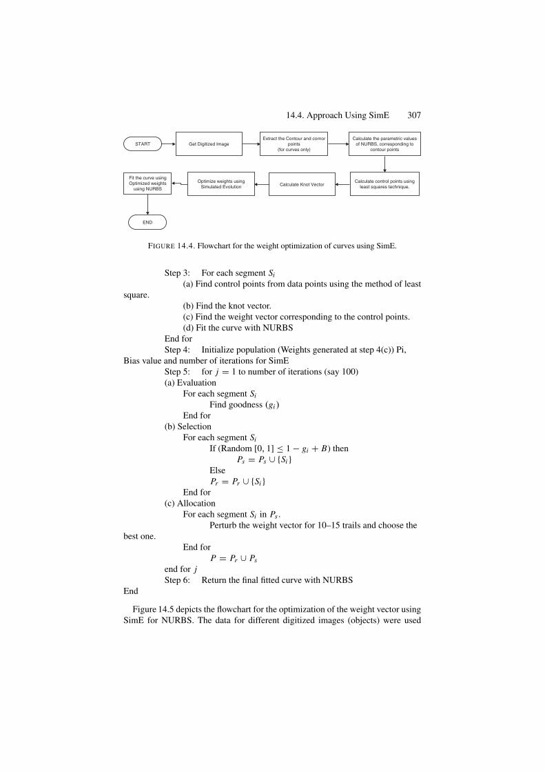
14.4. Approach Using SimE 307
START
END
Fit the curve usingOptimized weights
using NURBS
Get Digitized Image
Optimize weights usingSimulated Evolution
Calculate control points usingleast squares technique.Calculate Knot Vector
Calculate the parametric valuesof NURBS, corresponding to
contour points
Extract the Contour and cornorpoints
(for curves only)
FIGURE 14.4. Flowchart for the weight optimization of curves using SimE.
Step 3: For each segment Si(a) Find control points from data points using the method of least
square.(b) Find the knot vector.(c) Find the weight vector corresponding to the control points.(d) Fit the curve with NURBS
End forStep 4: Initialize population (Weights generated at step 4(c)) Pi,
Bias value and number of iterations for SimEStep 5: for j = 1 to number of iterations (say 100)(a) Evaluation
For each segment SiFind goodness (gi )
End for(b) Selection
For each segment SiIf (Random [0, 1] ≤ 1 − gi + B) then
Ps = Ps ∪ {Si }ElsePr = Pr ∪ {Si }
End for(c) Allocation
For each segment Si in Ps .Perturb the weight vector for 10–15 trails and choose the
best one.End for
P = Pr ∪ Psend for jStep 6: Return the final fitted curve with NURBS
End
Figure 14.5 depicts the flowchart for the optimization of the weight vector usingSimE for NURBS. The data for different digitized images (objects) were used
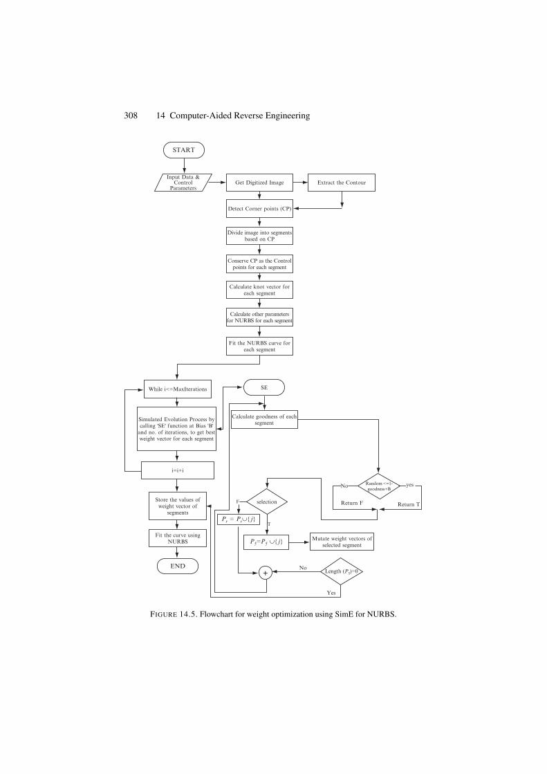
308 14 Computer-Aided Reverse Engineering
START
Get Digitized Image
Detect Corner points (CP)
Divide image into segmentsbased on CP
Conserve CP as the Controlpoints for each segment
Calculate knot vector foreach segment
Calculate other parametersfor NURBS for each segment
Fit the NURBS curve foreach segment
Calculate goodness of eachsegment
Random <=1-goodness+B
yesNo
selection
T
F Return F
Mutate weight vectors ofselected segment
Length (P5)=0
Pr = Pr∪{ j}
P5=P5 ∪{ j}
Yes
No
Return T
While i<=MaxIterations
i=i+i
END
Fit the curve usingNURBS
Store the values ofweight vector of
segments
Simulated Evolution Process bycalling 'SE' function at Bias 'B'
and no. of iterations, to get bestweight vector for each segment
SE
Extract the ContourInput Data &
ControlParameters
+
FIGURE 14.5. Flowchart for weight optimization using SimE for NURBS.
14.4. Approach Using SimE 309
to test the weight optimization of the NURBS curve using the SimE technique.Digitized image data is segmented using corner points. Each segment has its ownweight vector for fitting NURBS. The length of the weight vector equals the num-ber of control points generated using the least square technique for that segment.Experience has shown that using the fewest number of control points yields thefairest curve. Keeping this in mind for each segment, the number of control pointstaken is equal to the order of the curve. Table 14.3 shows the various parametersused and generated in the optimization of weight using SimE.
14.4.4 DemonstrationFigure 14.5 depicts the flowchart for the optimization of weight vector using SimEfor NURBS. The data for different digitized images (objects) were used to testthe weight optimization of NURBS curve using SimE technique. Digitized imagedata is segmented using corner points. Each segment has its own weight vectorfor fitting NURBS. The length of the weight vector equals the number of controlpoints generated using the least square technique for that segment. Experiencehas shown that using the fewest number of control points yields the fairest curve.Keeping this in mind for each segment, the number of control points taken is equalto the order of the curve. Table 14.3 shows various parameters used and generatedin the optimization of weight using SimE.
Figure 14.6 demonstrates the optimization results for the object “fork” inFigure 14.1(b) when a smaller set of corner points is achieved; see Figure 14.2(a),for the setting of parameter choice I in Table 14.1. Figure 14.6(a) represents thedefault curve. Figures 14.6(b) and 14.6(c) demonstrate the intermediate results forSimE curve fitting obtained for the object “fork” at iterations 1 and 40. respec-tively. The final NURBS fitted image for object fork, after 60 iterations, is shownin Figure 14.6(d). The algorithm converged at the 60th iteration for the object“fork.” The sum square error (SSE) between the boundary of the image object“fork” and the NURBS fitted curve with respect to the number of iterations is asshown in Figure 14.7. Average goodness of the fitted curve is shown in Figure 14.8.The number of segments selected for each iteration is plotted in Figure 14.9. Theresults obtained using the proposed algorithm are found to be better compared tothe results obtained using the genetic algorithm discussed in [9].
Figure 14.10 demonstrates the optimization results for the object “fork” inFigure 14.1(b) when a bigger set of corner points was achieved, see Figure 14.2(b),for the setting of parameter choice II in Table 14.1. Figure 14.10(a) represents thedefault curve. Figures 14.10(b) and 14.10(c) demonstrate the intermediate results
TABLE 14.3. Parameters used for weight optimization.
Image Order of NURBS No. of control points Bias value (B)(for each segment)
Fork 4 4 −0.5
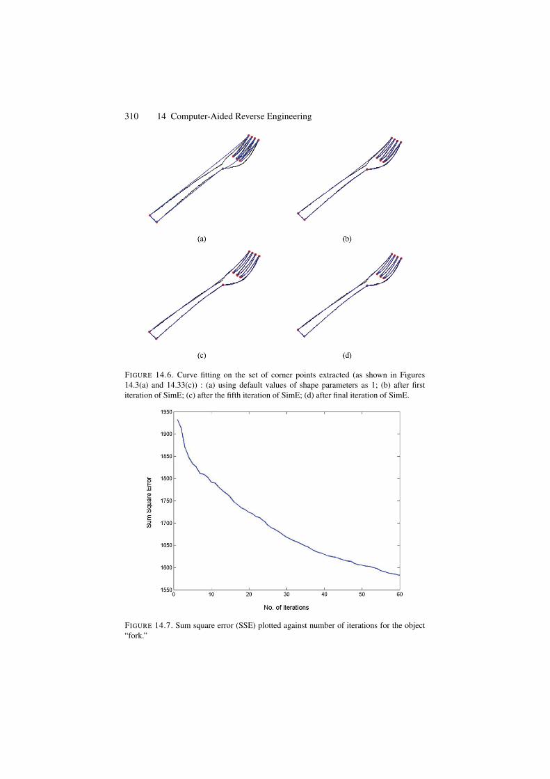
310 14 Computer-Aided Reverse Engineering
FIGURE 14.6. Curve fitting on the set of corner points extracted (as shown in Figures14.3(a) and 14.33(c)) : (a) using default values of shape parameters as 1; (b) after firstiteration of SimE; (c) after the fifth iteration of SimE; (d) after final iteration of SimE.
FIGURE 14.7. Sum square error (SSE) plotted against number of iterations for the object“fork.”
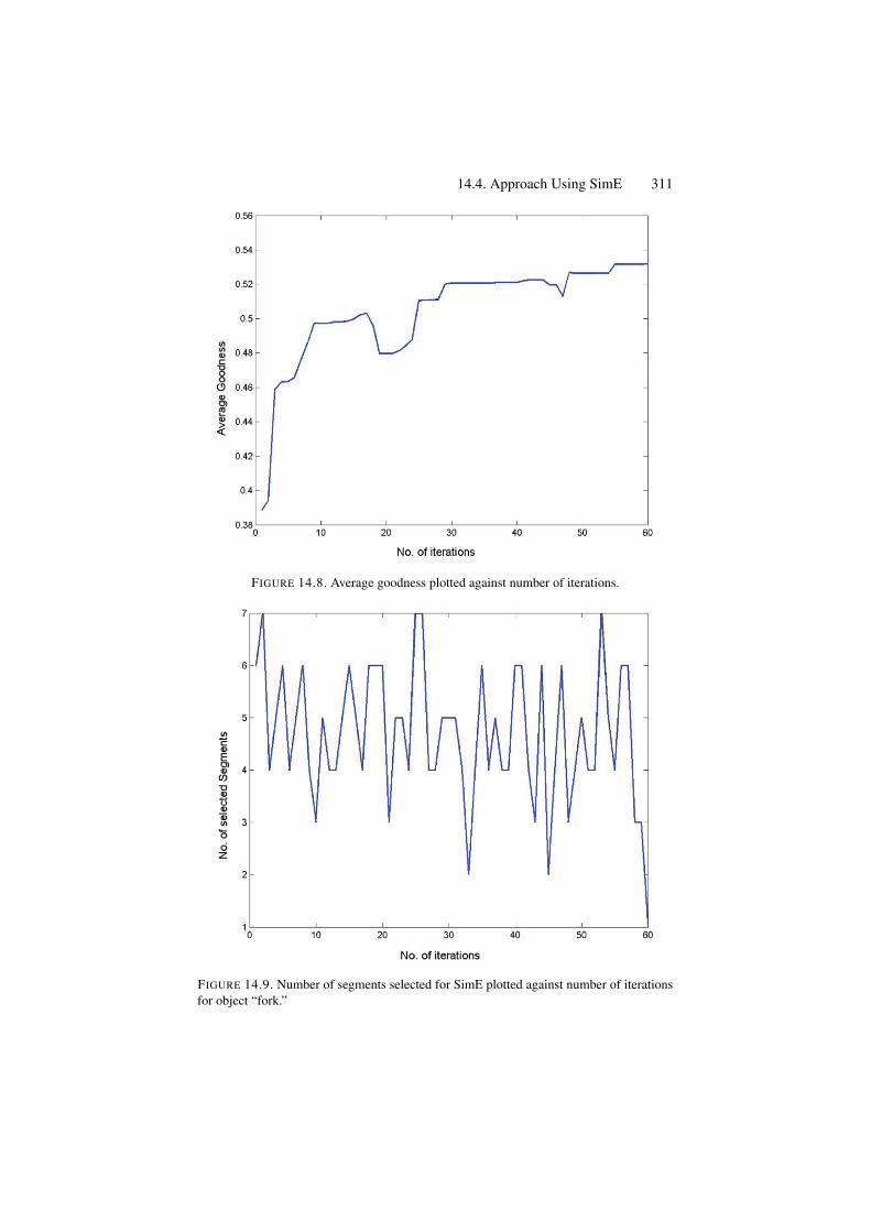
14.4. Approach Using SimE 311
FIGURE 14.8. Average goodness plotted against number of iterations.
FIGURE 14.9. Number of segments selected for SimE plotted against number of iterationsfor object “fork.”
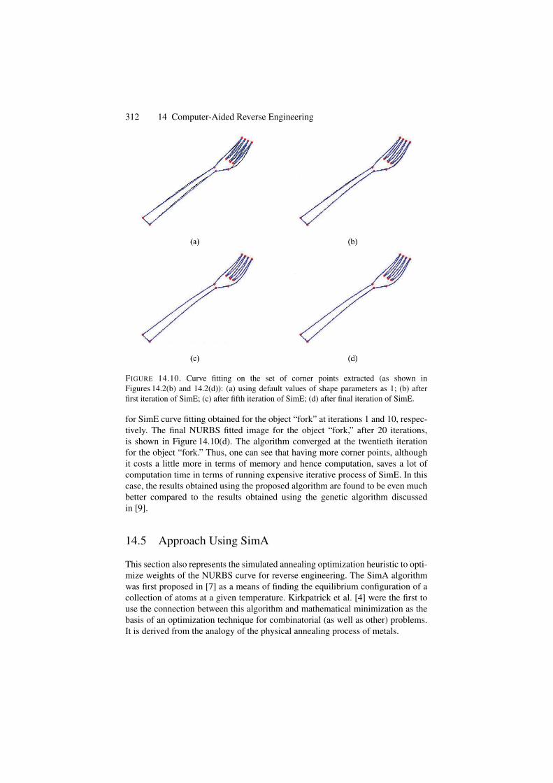
312 14 Computer-Aided Reverse Engineering
FIGURE 14.10. Curve fitting on the set of corner points extracted (as shown inFigures 14.2(b) and 14.2(d)): (a) using default values of shape parameters as 1; (b) afterfirst iteration of SimE; (c) after fifth iteration of SimE; (d) after final iteration of SimE.
for SimE curve fitting obtained for the object “fork” at iterations 1 and 10, respec-tively. The final NURBS fitted image for the object “fork,” after 20 iterations,is shown in Figure 14.10(d). The algorithm converged at the twentieth iterationfor the object “fork.” Thus, one can see that having more corner points, althoughit costs a little more in terms of memory and hence computation, saves a lot ofcomputation time in terms of running expensive iterative process of SimE. In thiscase, the results obtained using the proposed algorithm are found to be even muchbetter compared to the results obtained using the genetic algorithm discussedin [9].
14.5 Approach Using SimA
This section also represents the simulated annealing optimization heuristic to opti-mize weights of the NURBS curve for reverse engineering. The SimA algorithmwas first proposed in [7] as a means of finding the equilibrium configuration of acollection of atoms at a given temperature. Kirkpatrick et al. [4] were the first touse the connection between this algorithm and mathematical minimization as thebasis of an optimization technique for combinatorial (as well as other) problems.It is derived from the analogy of the physical annealing process of metals.
14.5. Approach Using SimA 313
14.5.1 Outline of SimESimA’s major advantage over other methods is its ability to avoid being trappedin local minima. The algorithm employs a random search, which not only acceptschanges that decrease the objective function E , but also some changes that wouldincrease it. The latter are accepted with a probability
Prob(accept) = exp(−�E/T ),
where �E is the increase in E and T is a control parameter, which by analogywith the original application is known as the system “temperature,” irrespective ofthe objective function involved.
SimA can be briefly described as follows: Given a function to optimize, andsome initial values for the variables (initial solution), SimA starts initially with ahigh temperature and a solution (or state). Based on the actual solution, it selectsa new random tentative solution in the neighborhood of the actual solution. Thetentative solution is generated by a small perturbation of the actual solution. Ifthe tentative solution has lower objective function value, then it is accepted as thenew solution. On the other hand, if the objective function value is high, it mightstill be accepted based on certain probability depending on the change in the valueof the objective function and the temperature. This process is repeated slowly bydecreasing the temperature until the optimized solution is reached. More detailsof SimA are given in Section 14.5.1 and can also be found in [19].
In order to implement simulated annealing, we need to formulate a suitable costfunction for the problem being solved. In addition, as in the case of local searchtechniques, we assume the existence of a neighborhood structure, and need theneighbor function to generate new states (neighborhood states) from current states.And, finally, we need a cooling schedule that describes the temperature parameterT and gives rules for lowering it.
14.5.2 Problem MappingThis section focuses on the organization of all the phases toward the achievementof outline capture of planar images. In particular, a detailed study is made to dis-cuss how the weights and knots, in the description of NURBS, can be optimizedin an independent manner. We start with the digitized image obtained from anelectronic device or scanner. The contour of the digitized image is extracted usingthe boundary detection algorithm [8], discussed in Section 14.3. This algorithmreturns a number of segments and, for each segment, a number of boundary points(data points) and their values.
14.5.2.1 Weight Optimization Using SimA
There are three commonly used methods to parameterize knots (the equally spacedmethod, the chord length method and the centripetal method), which can be uti-lized to identify knots. In this research, we use the chord length method. Assume
314 14 Computer-Aided Reverse Engineering
that the parameter value t lies between zero and one. For the set of the availabledata points, the maximum value of the knot vector, say at the � th data point, isdenoted by tmax.
t1 = 0,
t�tmax
=
�∑
s=2|Ds − Ds−1|
j∑
s=2|Ds − Ds−1|
, � ≥ 2.
⎫⎪⎪⎪⎪⎪⎬
⎪⎪⎪⎪⎪⎭
(14.11)
The control points are calculated using the least squares technique as the nextstep. A fairer or smoother curve is obtained by specifying fewer control polygonpoints than data points, that is, 2 ≤ k ≤ n < j . Recalling that a matrix times itstranspose is always square, the control polygon for a curve that fairs or smoothensthe data is given by
[D] = [B] [P] ,
which implies[B]T [D] = [B]T [B] [P] .
Hence[P] =
[[B]T [B]
]−1[B]T [D] ,
where[D]T = [D1 (t1) D2 (t2) . . . D j
(t j)]
,
are data points, and[P]T = [P1 P2 . . . Pn+1
],
are the control points and [B] is the set of B-spline basis functions.The evaluation of the control points, by least squares approximation, can be
viewed as an initial estimation of the fitted curve. Further refinement can beobtained by optimizing the different NURBS parameters, such as the knot valuesand the weights in order to achieve better fitting accuracy. The error function (orcost function) between the measured points and the fitted curve is generally givenby the following equation:
E =( s∑
i=0
|Qi − S(α1, . . . , αn)|r /s
)1/r
, (14.12)
where Q represents the set of measured points of the target curve. S (α1. . .αn) isthe geometric model of the fitted curve, where (α1, . . . , αn) are the parameters ofthe fitted curve; s is the number of measured points and r is an exponent rang-ing from 1 to infinity. The fitting task can then be viewed as the optimization ofthe curve parameters (α1, . . . , αn) to minimize the error (or cost) E . In case theexponent r is equal to 2, the above equation reduces to the least squares function.It is to be noted that the weights present a large number of independent variables(equaling the number of control points) to the optimization problem, which maylead to a large search space. Therefore, global optimization techniques are neededfor optimizing such problems.
14.5. Approach Using SimA 315
We describe, in this section, the use of SimE optimization heuristic to optimizeweights of the NURBS curve. The initial solution S0 of weight vector is randomlyselected from the range [0, 0.5]. The number of elements in the weight vectorcorresponds to the number of control points. The cooling schedule used here ispresented similar to the one in [4]. It is based on the idea that the initial tempera-ture T0 must be large to virtually accept all transitions and that the changes in thetemperature at each invocation of the Metropolis loop are small. The scheme pro-vides guidelines to the choice of T0, the rate of decrements of T , the terminationcriterion and the length of the Markov chain (M).
14.5.2.2 Initial Temperature T0
The initial temperature must be chosen so that almost all transitions are acceptedinitially. That is, the initial acceptance ratio χ(T0) must be close to unity where
χ (T0) = Number of moves accepted at T0
Total number of moves attempted at T0.
To determine T0, we start off with a small value of initial temperature given byT ′
0, in the Metropolis function. Then χ(T ′0) is computed. If χ(T ′
0) is not close tounity, then T ′
0 is increased by multiplying it by a constant factor larger than one.The above procedure is repeated until the value of χ(T ′
0) approaches unity. Thevalue of T ′
0 is then the required value of T0.
14.5.2.3 Decrement of T
A decrement function is used to reduce the temperature in a geometric progression,and is given by
Tk+1 = αTk, k = 0, 1, . . . ,
where α is a positive constant less than one, since successive temperatures aredecreasing. Further, since small changes are desired, the value of α is chosen veryclose to unity, typically 0.8 ≤ α ≤ 0.99.
14.5.2.4 Length of Markov Chain M
The length of Markov chain M is equivalent to the number of times the Metropolisloop is executed at a given temperature. If the optimization process begins with ahigh value of T0, the distribution of relative frequencies of states will be veryclose to the stationary distribution. In such a case, the process is said to be inquasi-equilibrium. The number M is based on the requirement that at each valueof Tk quasi-equilibrium is restored.
Since at decreasing temperatures uphill transitions are accepted with decreasingprobabilities, one has to increase the number of iterations of the Metropolis loopwith decreasing T (so that the Markov chain at that particular temperature willremain irreducible and with all states being non null). A factor β is used (β > 1)which, in a geometric progression, increases the value of M . That is, each time theMetropolis loop is called, T is reduced to αT and M is increased to βM .
316 14 Computer-Aided Reverse Engineering
14.5.2.5 Weight Seclection
The neighborhood of each element of the weight vector is randomly selectedwithin a range of [weight element value, weight element value + 1]. Since thenumber of elements of the weight vector equals the number of control points, thisrange is selected in order to optimize the locality of the search. The details of theimplementation are as follows:
First of all, construct an initial NURBS curve using the weights, knots and themeasured control points. The initial solution S0 (NewS) of weight vector is cur-rently assigned to the best solution (BestS). In the next step, we call Metropolisiteration. In this step, we measure the value of cost function E (CurCost) andassign a new cost. After perturbing the elements of the weight vector in a smallneighborhood ([wcur
i , wcuri + 1] where wcur
i is the current weight correspondingto the control point i), we calculate again the cost function E for the newly fittedcurve as NewCost. If the value of CurCost is less than NewCost, we assign thecurrent cost value as the new cost and weight vector corresponding to this costas the best solution (BestS). If the CurCost value is higher than in the compari-son with NewCost, that means the perturb solution is worse than the original one.In this case, we accept the new solution only on probability basis, that is, a ran-dom number is generated between 0 and 1. If the generated random number issmaller than e
CurCost−NewCostT , where T is the current temperature, then we keep the
new settings. Otherwise, we neglect the perturb solution. This process is repeatedslowly by decreasing the temperature until the optimized solution is reached. Theflowchart for the NURBS curve approximation, based on simulated annealing, isshown in Figure 14.11.
14.5.3 DemonstrationThis section is meant for the demonstration of results achieved during the imple-mentation of the SimA scheme. Some discussion is also made on the merits anddemerits of the schemes. We used the bitmap images as the input to the algorithmfor weight optimization of NURBS for curves. The general parameters taken forcurves are described as follows: While cooling, since small changes in tempera-tures are desired, we have chosen the value of α as 0.99, which is close to unity.Since the value of β should be greater than 1, a value of 1.5 is chosen. The algo-rithm executes the Metropole function, based on Maxtime, which is set to 250.The order k is chosen to be 4. The number of control points have been taken as70. These are the default settings and hence can be changed by the users whendesired.
Figure 14.18 shows the calculation of the best cost by the SimA heuristic whenapproximated the outline in Figure 14.13 of the pound image in Figure 14.12.Figures 14.14–14.17 depict the intermediate fittings of the “pound” symbol forweight optimization at various iterations. A gradual decrease in the (current) costfunction can be viewed in Figure 14.18. Figure 14.18 also shows that (current)costs are selected for the next iteration, even if previous (current) costs were better,to avoid getting trapped in the local minimum.
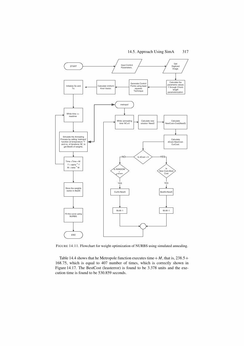
14.5. Approach Using SimA 317
START Input ControlParameters.
Calculate theparametric values‘t’ through Chord-
lengthparameterization.
Initialize So andTo.
While time <=maxtime
Simulate the AnnealingProcess by calling ‘metropol’function at temperature ‘T’and no. of iterations ‘M’, to
get BestS of weights.
Time =Time +M
T = alpha * TM = beta * M
Store the weightsvector in BestS
Fit the curve usingNURBS.
END
While (annealingtime ‘M’)>0
Calculate newsolution ‘NewS’
CalculateNewCost=Cost(NewS)
CalculatedCost=NewCost-
CurCost.
Is dCost < 0
Is RANDOM<
e(-dCost/T)
IsNew Cost<Best
Cost
YESNO
BestS=NewS
YES
M=M−1
CurS=NewS
YES
M=M−1
metropol
Generate ControlPoints using least
squaresTechnique
Calculate UniformKnot Vector.
GetDigitizedImage.
FIGURE 14.11. Flowchart for weight optimization of NURBS using simulated annealing.
Table 14.4 shows that he Metropole function executes time+ M , that is, 238.5+168.75, which is equal to 407 number of times, which is correctly shown inFigure 14.17. The BestCost (leasterror) is found to be 3.378 units and the exe-cution time is found to be 530.859 seconds.
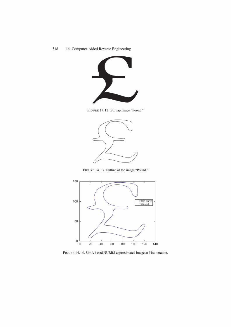
318 14 Computer-Aided Reverse Engineering
FIGURE 14.12. Bitmap image “Pound.”
FIGURE 14.13. Outline of the image “Pound.”
00 20 40 60 80 100 120 140
50
100
150
Fitted CurveTime=51
FIGURE 14.14. SimA based NURBS approximated image at 51st iteration.
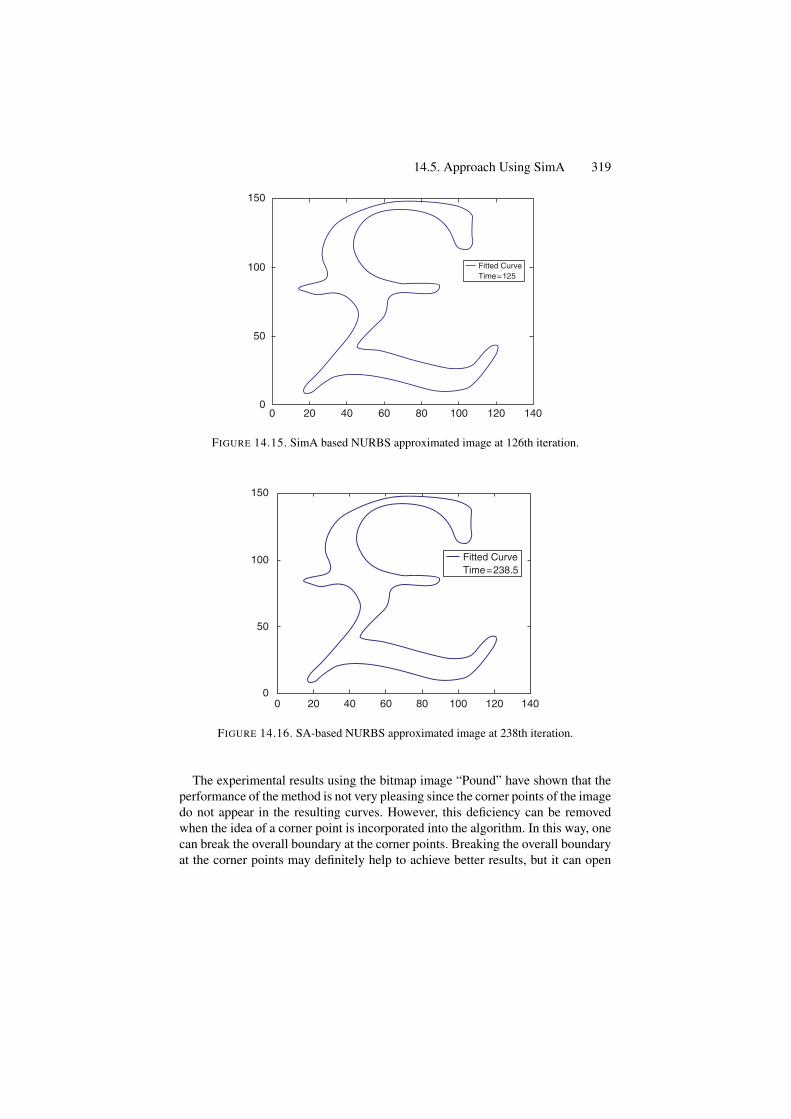
14.5. Approach Using SimA 319
00 20 40 60 80 100 120 140
50
100
150
Fitted CurveTime=125
FIGURE 14.15. SimA based NURBS approximated image at 126th iteration.
00 20 40 60 80 100 120 140
50
100
150
Fitted CurveTime=238.5
FIGURE 14.16. SA-based NURBS approximated image at 238th iteration.
The experimental results using the bitmap image “Pound” have shown that theperformance of the method is not very pleasing since the corner points of the imagedo not appear in the resulting curves. However, this deficiency can be removedwhen the idea of a corner point is incorporated into the algorithm. In this way, onecan break the overall boundary at the corner points. Breaking the overall boundaryat the corner points may definitely help to achieve better results, but it can open
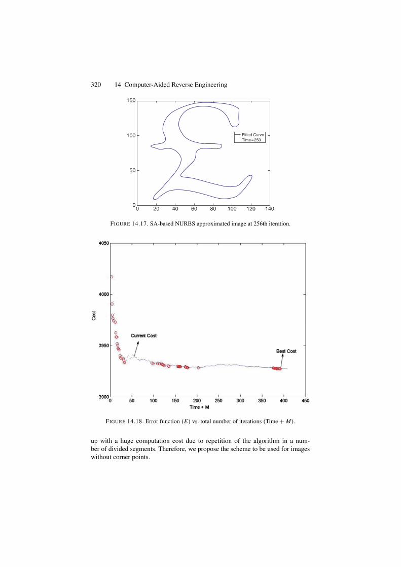
320 14 Computer-Aided Reverse Engineering
00 20 40 60 80 100 120 140
50
100
150
Fitted CurveTime=250
FIGURE 14.17. SA-based NURBS approximated image at 256th iteration.
FIGURE 14.18. Error function (E) vs. total number of iterations (Time + M).
up with a huge computation cost due to repetition of the algorithm in a num-ber of divided segments. Therefore, we propose the scheme to be used for imageswithout corner points.
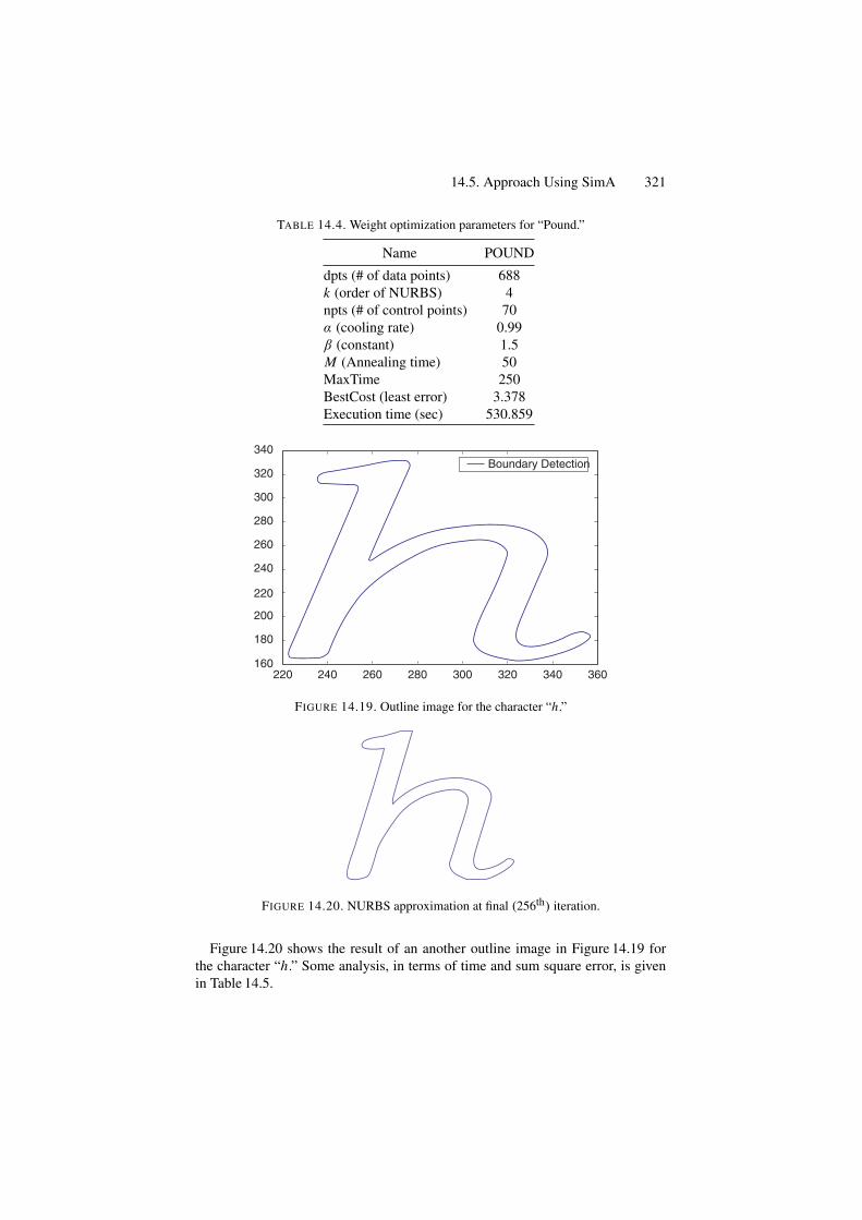
14.5. Approach Using SimA 321
TABLE 14.4. Weight optimization parameters for “Pound.”
Name POUND
dpts (# of data points) 688k (order of NURBS) 4npts (# of control points) 70α (cooling rate) 0.99β (constant) 1.5M (Annealing time) 50MaxTime 250BestCost (least error) 3.378Execution time (sec) 530.859
340
320
300
280
260
240
220
200
180
160220 240 260 280 300 320 340
Boundary Detection
360
FIGURE 14.19. Outline image for the character “h.”
FIGURE 14.20. NURBS approximation at final (256th) iteration.
Figure 14.20 shows the result of an another outline image in Figure 14.19 forthe character “h.” Some analysis, in terms of time and sum square error, is givenin Table 14.5.
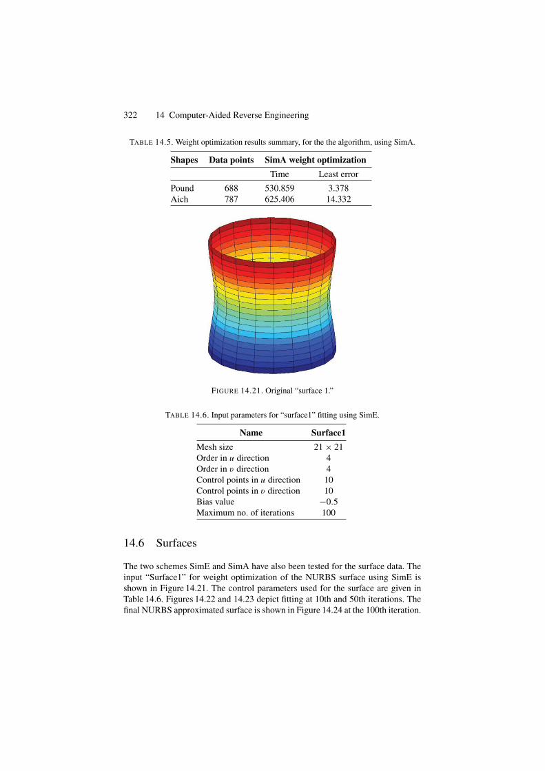
322 14 Computer-Aided Reverse Engineering
TABLE 14.5. Weight optimization results summary, for the the algorithm, using SimA.
Shapes Data points SimA weight optimizationTime Least error
Pound 688 530.859 3.378Aich 787 625.406 14.332
FIGURE 14.21. Original “surface 1.”
TABLE 14.6. Input parameters for “surface1” fitting using SimE.
Name Surface1Mesh size 21 × 21Order in u direction 4Order in v direction 4Control points in u direction 10Control points in v direction 10Bias value −0.5Maximum no. of iterations 100
14.6 Surfaces
The two schemes SimE and SimA have also been tested for the surface data. Theinput “Surface1” for weight optimization of the NURBS surface using SimE isshown in Figure 14.21. The control parameters used for the surface are given inTable 14.6. Figures 14.22 and 14.23 depict fitting at 10th and 50th iterations. Thefinal NURBS approximated surface is shown in Figure 14.24 at the 100th iteration.
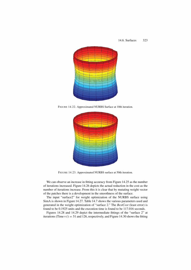
14.6. Surfaces 323
FIGURE 14.22. Approximated NURBS Surface at 10th iteration.
FIGURE 14.23. Approximated NURBS surface at 50th iteration.
We can observe an increase in fitting accuracy from Figure 14.25 as the numberof iterations increased. Figure 14.26 depicts the actual reduction in the cost as thenumber of iterations increase. From this it is clear that by mutating weight vectorof the patches there is a development in the smoothness of the surface.
The input “surface2” for weight optimization of the NURBS surface usingSimA is shown in Figure 14.27. Table 14.7 shows the various parameters used andgenerated in the weight optimization of “surface 2.” The BestCost (least error) isfound to be 0.1925 units and the execution time is found to be 117.016 seconds.
Figures 14.28 and 14.29 depict the intermediate fittings of the “surface 2” atiterations (Time+i) = 51 and 126, respectively, and Figure 14.30 shows the fitting
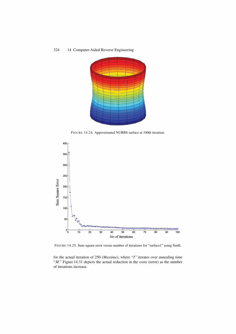
324 14 Computer-Aided Reverse Engineering
FIGURE 14.24. Approximated NURBS surface at 100th iteration.
FIGURE 14.25. Sum square error versus number of iterations for “surface1” using SimE.
for the actual iteration of 250 (Maxtime), where “I ” iterates over annealing time“M .” Figure 14.31 depicts the actual reduction in the costs (error) as the numberof iterations increase.
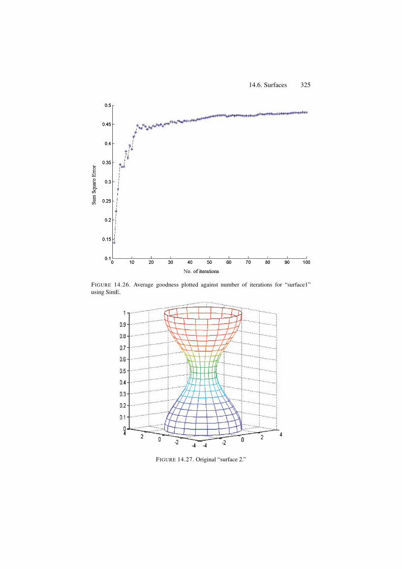
14.6. Surfaces 325
FIGURE 14.26. Average goodness plotted against number of iterations for “surface1”using SimE.
FIGURE 14.27. Original “surface 2.”
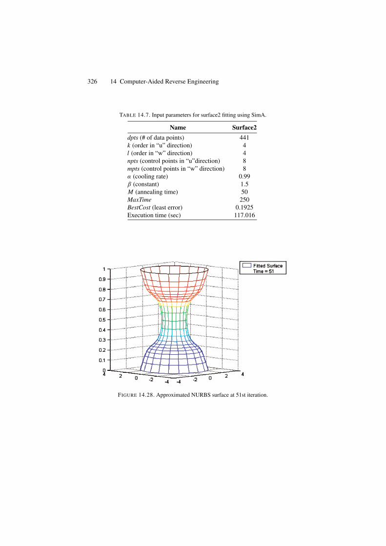
326 14 Computer-Aided Reverse Engineering
TABLE 14.7. Input parameters for surface2 fitting using SimA.
Name Surface2dpts (# of data points) 441k (order in “u” direction) 4l (order in “w” direction) 4npts (control points in “u”direction) 8mpts (control points in “w” direction) 8α (cooling rate) 0.99β (constant) 1.5M (annealing time) 50MaxTime 250BestCost (least error) 0.1925Execution time (sec) 117.016
FIGURE 14.28. Approximated NURBS surface at 51st iteration.
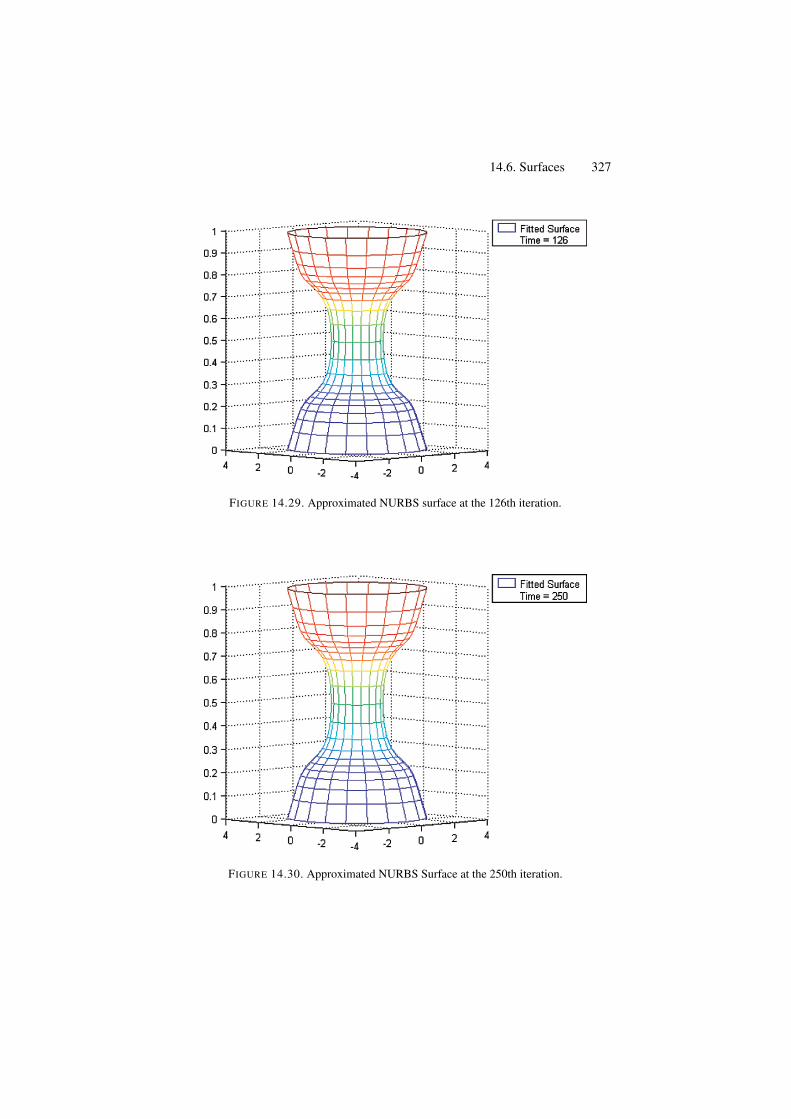
14.6. Surfaces 327
FIGURE 14.29. Approximated NURBS surface at the 126th iteration.
FIGURE 14.30. Approximated NURBS Surface at the 250th iteration.
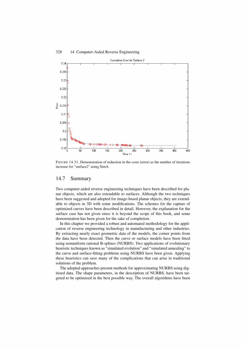
328 14 Computer-Aided Reverse Engineering
FIGURE 14.31. Demonstration of reduction in the costs (error) as the number of iterationsincrease for “surface2” using SimA.
14.7 Summary
Two computer-aided reverse engineering techniques have been described for pla-nar objects, which are also extendable to surfaces. Although the two techniqueshave been suggested and adopted for image-based planar objects, they are extend-able to objects in 3D with some modifications. The schemes for the capture ofoptimized curves have been described in detail. However, the explanation for thesurface case has not given since it is beyond the scope of this book, and somedemonstration has been given for the sake of completion.
In this chapter we provided a robust and automated methodology for the appli-cation of reverse engineering technology in manufacturing and other industries.By extracting nearly exact geometric data of the models, the corner points fromthe data have been detected. Then the curve or surface models have been fittedusing nonuniform rational B-splines (NURBS). Two applications of evolutionaryheuristic techniques known as “simulated evolution” and “simulated annealing” tothe curve and surface-fitting problems using NURBS have been given. Applyingthese heuristics can save many of the complications that can arise in traditionalsolutions of the problem.
The adopted approaches present methods for approximating NURBS using dig-itized data. The shape parameters, in the description of NURBS, have been tar-geted to be optimized in the best possible way. The overall algorithms have been
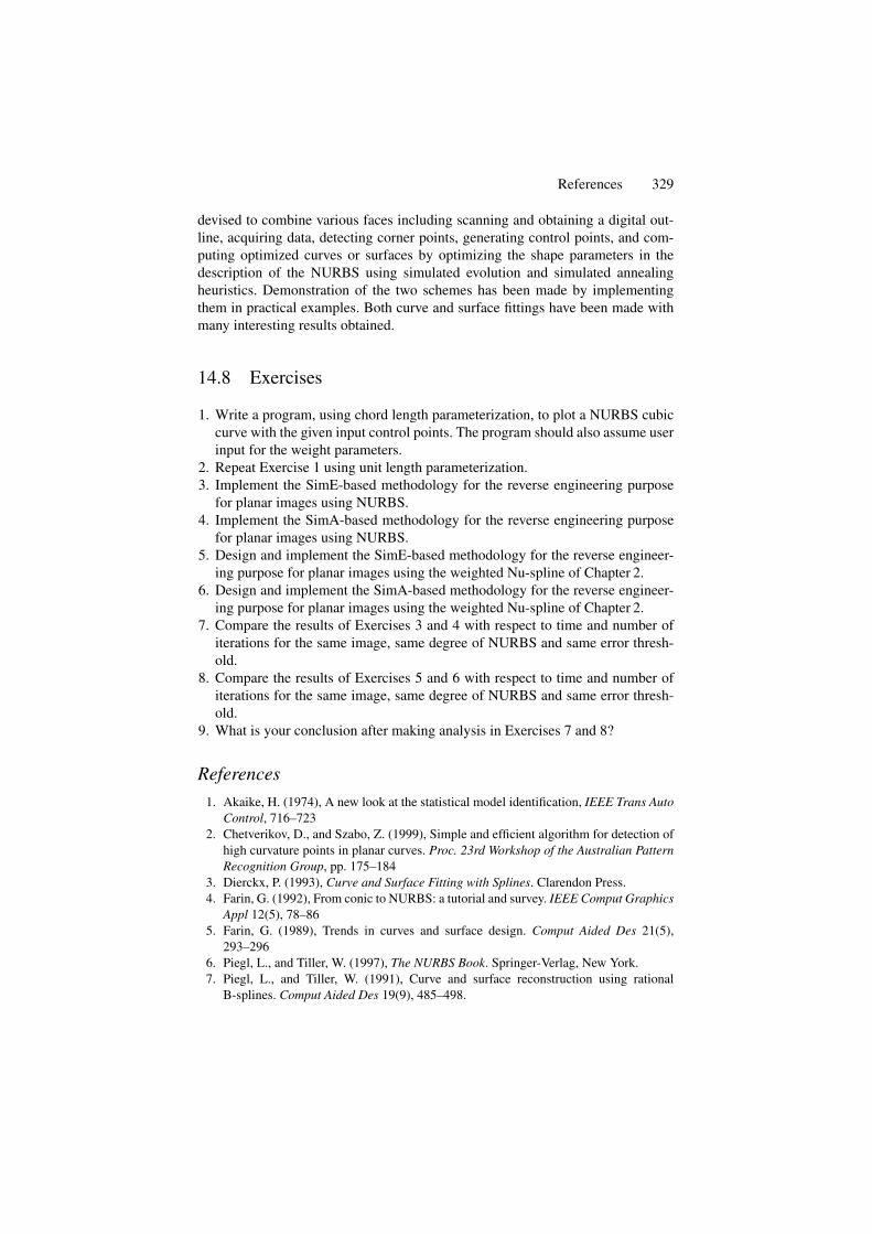
References 329
devised to combine various faces including scanning and obtaining a digital out-line, acquiring data, detecting corner points, generating control points, and com-puting optimized curves or surfaces by optimizing the shape parameters in thedescription of the NURBS using simulated evolution and simulated annealingheuristics. Demonstration of the two schemes has been made by implementingthem in practical examples. Both curve and surface fittings have been made withmany interesting results obtained.
14.8 Exercises
1. Write a program, using chord length parameterization, to plot a NURBS cubiccurve with the given input control points. The program should also assume userinput for the weight parameters.
2. Repeat Exercise 1 using unit length parameterization.3. Implement the SimE-based methodology for the reverse engineering purpose
for planar images using NURBS.4. Implement the SimA-based methodology for the reverse engineering purpose
for planar images using NURBS.5. Design and implement the SimE-based methodology for the reverse engineer-
ing purpose for planar images using the weighted Nu-spline of Chapter 2.6. Design and implement the SimA-based methodology for the reverse engineer-
ing purpose for planar images using the weighted Nu-spline of Chapter 2.7. Compare the results of Exercises 3 and 4 with respect to time and number of
iterations for the same image, same degree of NURBS and same error thresh-old.
8. Compare the results of Exercises 5 and 6 with respect to time and number ofiterations for the same image, same degree of NURBS and same error thresh-old.
9. What is your conclusion after making analysis in Exercises 7 and 8?
References1. Akaike, H. (1974), A new look at the statistical model identification, IEEE Trans Auto
Control, 716–7232. Chetverikov, D., and Szabo, Z. (1999), Simple and efficient algorithm for detection of
high curvature points in planar curves. Proc. 23rd Workshop of the Australian PatternRecognition Group, pp. 175–184
3. Dierckx, P. (1993), Curve and Surface Fitting with Splines. Clarendon Press.4. Farin, G. (1992), From conic to NURBS: a tutorial and survey. IEEE Comput Graphics
Appl 12(5), 78–865. Farin, G. (1989), Trends in curves and surface design. Comput Aided Des 21(5),
293–2966. Piegl, L., and Tiller, W. (1997), The NURBS Book. Springer-Verlag, New York.7. Piegl, L., and Tiller, W. (1991), Curve and surface reconstruction using rational
B-splines. Comput Aided Des 19(9), 485–498.
330 14 Computer-Aided Reverse Engineering
8. Quddus, A., (1998), Curvature Analysis Using Multi-resolution Techniques. PhDThesis. Department of Electrical Engineering, King Fahd University of Petroleum &Minerals, Dhahran, Saudi Arabia.
9. Sarfraz, M., and Raza, S.A. (2001), Capturing outline of fonts using genetic algo-rithm and splines. The Proceedings of IEEE International Conference on InformationVisualization-IV’2001-UK, IEEE Computer Society Press, 738–743.
10. Sarfraz, M., Raza, S.A. and Baig, M.H. (2005), Computing Optimized Curves withNURBS Using Evolutionary Intelligence, Lecture Notes in Computer Science, Vol.3480: Computational Science and Its Applications. Gervasi, O., Gavrilova, M.L.,Kumar, V., Lagana, A., Lee, H.P., Mun, Y., and Taniar, D., eds., Springer-Verlag,New York, pp. 806–815.
11. Kling, R.M., and Benerjee, P. (1991), Empirical and theoretical studies of simu-lated evolution method applied to standard cell placement. IEEE Trans Comput AidedDesign 10(10).
12. Sarfraz, M., Riyazuddin, M., and Baig, M.H. (2005), Capturing planar shapes byapproximating their outlines, Int J Computational Appl Math, Elsevier Science.
13. Sarfraz, M., Sait, Sadiq, M., Balah, M., and Baig, M.H. (2006), Computing optimizedNURBS curves using simulated evolution on control parameters, applications of softcomputing: recent trends. In: Advances in Soft Computing, Tiwari, A., Knowles,J., Avineri, E., Dahal, K., and Roy, R., eds., Springer-Verlag New York, pp. 35–44.
14. Youssef, M. (2001), Reverse Engineering of Geometric Surfaces Using Tabu SearchOptimization Technique. Master Thesis, Cairo University, Egypt.
15. Yau, H.-T., and Chen, J.-S., (1997), Reverse engineering of complex geometry usingrational B-splines, Int J Adv Manufacturing Technol 13(8), 548–555.
16. Cho, M.-W., Seo, T.-I., Kim, J.-D., and Kwon, O.-Y. (2000), Reverse engineering ofcompound surfaces using boundary detection method, Korean Soc Mech Eng Int J14(10), 1104–1113.
17. Pratt, M.J., Goult, R.J., and Ye, L. (1993), On rational parametric curve approximation,Comput Aided Geom Des 10, 363–377.
18. Laurent-Gengoux, P., and Mekhilef, M. (1993), Optimization of a NURBS represen-tation, Comput Aided Des 25(11), 699–710.
19. Sarfraz, M. (2006), Computer-aided reverse engineering using simulated evolution onNURBS, Int J Virtual Phys Prototyping, Taylor & Francis, 1(4), 494–512.
15Multiresolution Frameworkfor B-Splines
Abstract. The piecewise polynomial B-spline representation is a flexible tool in CAGD forrepresenting and designing geometric objects. In the field of computer graphics (CG),computer-aided design (CAD), or computer-aided engineering (CAE), a very usefulproperty for a given spline model is to have locally supported basis functions. Thisallows localized modification of the shape. Unfortunately this property can also become aserious disadvantage when the user wishes to edit the global shape of a complex object.Multiresolution representation is proposed as a solution to alleviate this problem. Variousmultiresolution methods are described for different B-spline models.
15.1 Introduction
In the field of geometric modeling, the construction of efficient, intuitive and inter-active editors for geometric objects is a fundamental objective, but it is still adifficult challenge. In many freeform geometric modeling systems the users areallowed to work in the framework of a specific data model such as Bezier ornonuniform rational B-splines [6]. This imposes constraints on the set of geo-metric manipulation operations that can be performed, the man-machine interfaceand the type of objects that can be modeled.
There are various curve manipulation techniques proposed in the current liter-ature [1–21]. The Euclidean distances between the point of modification and thecontrol points of a B-spline curve were used as weights to affect the control pointsin [4]. The difficulty with this approach appears when the two separate portionsof the curve are close. To alleviate the difficulty in editing freeform shapes whilematching engineering specifications, constraint-based approaches have been pro-posed in [2, 22]. Direct and interactive manipulation tools of freeform curves andsurfaces are investigated in [5].
In the field of computer graphics or computer-aided design, a very useful prop-erty for a given spline model is to have locally supported basis functions. Thisproperty allows localized modifications of the shape. Unfortunately this propertycan also become a serious disadvantage when the user wishes to edit the global
331
332 15. Multiresolution Framework for B-Splines
shape of a complex object. Piecewise polynomial B-spline representation is com-mon in many contemporary geometric modeling systems. While this is a powerfultool with many desirable properties, the same properties impose some undesirableconstraints on the user. For example, the most attractive property, locality, restrictsthe user to perform global operations on the object being modeled. To perform aglobal operation, it has to be transformed into a series of local operations affectingonly a small portion of the curve, which makes the process time a waste and preci-sion hazardous [12]. The ability to simultaneously perform both local and globaloperations at will would add significant functionality to any modeling system.
Multiresolution representation is a possible solution that addresses this prob-lem, because it allows the user to edit objects at different resolution levels. Bothlocal and global operations can be performed on curves by representing themusing multiresolution decomposition. Several approaches have been proposed formultiresolution representation of splines, mostly based on wavelets. All theseapproaches involve expensive precalculations in the case of curves and surfaces.It often requires specific treatment of boundary control points. Moreover, theseapproaches depend on the given spline model they manipulate. The whole schemehas to be redefined when it comes to manipulating other spline models; only thephilosophy of the calculus can potentially be reused [12].
All the approaches presented are either for the uniform B-splines or nonuniformB-splines (NUBS). NUBS are useful because:
• By manipulating the control points, knot vector and weights, NUBS providesthe facility to design a large variety of shapes.
• They offer a common mathematical form for representing and designing bothstandard analytic shapes (conics, quadrics) and freeform curves and surfaces.
• Evaluation is reasonably fast and computationally stable.• NUBS have clear geometric tool kit (knot insertion/deletion, degree elevation,
etc.), which can be used to design, analyze, process and interrogate objects.
In this chapter, Section 15.2 describes the general theory of B-splines. InSection 15.3, we discuss two of the multiresolution representations presented forB-splines. Section 15.4 is about another method for multiresolution representationfor NUBS; it is based on control point decimation. This method, in Section 15.5,is demonstrated by means of graphics.
15.2 Theory of NUBS
The general expression for the calculation of coordinate positions along a B-splinecurve in a blending function formulation is of the form:
P(t) =n∑
i=0
Pi Bi,p(t), tmin ≤ t < tmax, 2 ≤ p ≤ n + 1,
where Pi is an input set of n+1 control points and the B-spline blending functionsBi,p are polynomials of degree p. The Cox Deboor [7, 13] recursive formula forthe B-spline basis can be defined as:
15.3. Multiresolution Representation of B-Splines 333
Bi,1(t) ={
1, if ti ≤ t ≤ ti+1
0, otherwise.
and
Bi,p(t) = (t − ti )Bi,p−1(t)ti+p−1 − ti
+ (ti+p − t)Bi+1,p−1(t)ti+p − ti+1
,
where a knot vector t = {t0, t1, . . . , tm} of m + 1 knots is assumed. NUBSare nonuniform B-splines and is the term given to curves that are defined on aknot vector where the interior knot spans are not equal. As an example, we mayhave interior knots with spans of zero. Some common curves require this type ofnonuniform knot spacing. The use of this option allows better shape control andthe ability to model a larger class of shapes.
15.3 Multiresolution Representation of B-Splines
In the fields of computer graphics or computer-aided design, a very useful prop-erty for a given spline model is to have locally supported basis functions in orderto allow localized modifications of the shape. Unfortunately, this property canalso become a serious disadvantage when the user wishes to edit the global shapeof a complex object. Piecewise polynomial B-spline representation is commonin many contemporary geometric modeling systems. While this is a powerful toolwith many desirable properties, the same properties impose some undesirable con-straints on the user. For example, the most attractive property, locality, restrictsthe user to perform global operations on the object being modeled. To perform aglobal operation, it has to be transformed into a series of local operations affectingonly a small portion of the curve, which makes the process a waste of and preci-sion hazardous [12]. The ability to simultaneously perform both local and globaloperations at will would add significant functionality to any modeling system.
Multiresolution representation is a possible solution that addresses this prob-lem, because it allows the user to edit objects at different resolution levels. Bothlocal and global operations can be performed on curves by representing them usingmultiresolution decomposition. Multiresolution analysis can be defined as an abil-ity to simultaneously perform both local and global operations on the analyzedobject [6]. Several approaches have been proposed for multiresolution representa-tion of splines, mostly based on wavelets. All these approaches involve expensiveprecalculations and in the case of open curves and surfaces, often require specifictreatment of boundary control points. Moreover, these approaches depend on thegiven spline model they manipulate; the whole scheme has to be redefined whenit comes to manipulating other spline models, only the philosophy of the calculuscan potentially be reused [12].
For the sake of completeness, two of the existing approaches for the multi-resolution representation of B-splines are briefly presented. One uses B-spline
334 15. Multiresolution Framework for B-Splines
wavelets for endpoint interpolating B-splines. Another deals with multiresolutioncontrol for nonuniform B-splines, which uses the knot decimation and leastsquares approximation.
15.3.1 Multiresolution Representation of B-SplinesUsing Wavelets
To understand the basic ideas behind wavelets and multiresolution analysis, con-sider a discrete signal Cn , expressed as column vector of samples. The samplescan be the control points of the curve if we want to create a low-resolution versionCn−1 of Cn with a fewer number of samples m′. The approach is to use some formof filtering and downsampling on m samples of Cn . This process can be expressedas the matrix equation:
Cn−1 = AnCn, (15.1)
where An is m′ × m matrix.Since Cn−1 contains fewer samples than Cn , it is clear that some amount of
detail is lost in the filtering process. If An is appropriately chosen, it is possible tocapture the lost details as another signal Dn−1, given as:
Dn−1 = BnCn, (15.2)
where Bn is (m − m′)× m matrix, which is related to matrix An . The matrices An
and Bn are called analysis filters. The process of splitting Cn into low-resolutionversion Cn−1 and detail Dn−1 is called decomposition.
If An and Bn are chosen correctly, the original signal Cn can be recovered fromCn−1 and Dn−1 by using another pair of matrices Pn and Qn as
Cn = PnCn−1 + Qn Dn−1, (15.3)
The recovery process of Cn from Cn−1 and Dn−1 is called reconstruction, and thepair of matrices Pn and Qn are called synthesis filters. The procedure of splittingCn into a low-resolution part Cn−1 and a detail part Dn−1 can be applied recur-sively to the new signal Cn−1. Thus, the original signal can be decomposed as ahierarchy of low-resolution signals C0, . . . , Cn−1 and details D0, . . . , Dn−1. Thisrecursive process is known as a filter bank.
Since the original signal Cn can be recovered from the sequence C0, D0, D1, . . . ,Dn−1, this sequence can be thought of as a transform of the original signal, knownas wavelet transform. The total size of the transform C0, D0, D1, . . . , Dn−1 is thesame as that of the original signal Cn , that is, no extra storage is required. For thedetailed description, refer to [19–21].
For performing the wavelet transform, all that is needed is an appropriate set ofanalysis and synthesis filters A j , B j , P j , and Q j . To construct these filters, eachsignal Cn is associated with a function f n(u) with u ∈ [0, 1] given by:
f n (u) = �n (u) Cn, (15.4)
15.3. Multiresolution Representation of B-Splines 335
where �n (u) is a row matrix of basis functions[φn
1 (u) , . . . , φn1 (u)
]called scal-
ing functions.The scaling functions are required to be refinable; that is, for all j in [1, n] a
matrix P j must exist such that
� j−1 = � j P j . (15.5)
Each scaling function at level j − 1 must be expressible as a linear combinationof finer scaling functions at level j .
Next, let V j be the linear space spanned by the set of scaling functions � j .From Equation (15.5), it is implied that these spaces are nested, that is, V 0 ⊂V 1 ⊂ . . . ⊂ V n . Choosing an inner product for the basis functions in V j allowsus to define W j as the orthogonal complement of V j in V j+1, that is, the spaceW j whose basis functions � j =
[ψn
1 (u) , . . . , ψnm−m′ (u)
]are such that � j and
� j together form a basis for V j+1, and every ψj
i (u) is orthogonal to every φji (u)
under the chosen inner product. The basis functions ψj
i (u) are called wavelets.The synthesis filter Q j can be constructed as the matrix that satisfies
� j−1 = � j Q j . (15.6)
The above two equations can be expressed as a single equation by concatenatingthe matrices together:
[� j−1|� j−1] = � j [P j |Q j ]. (15.7)
The analysis filters A j and B j are formed by the matrices satisfying the inverserelation:
The matrices [P j |Q j ] and [A j |B j ]T are both square matrices. Therefore, wehave the following:
[� j−1|� j−1][
A j
B j
]= � j ,
[A j
B j
]=[
P j |Q j]−1
.
15.3.2 Multiresolution of NUBS Using Knot DecimationAnother method described is for the multiresolution representation of nonuniformB-splines (NUBS) as presented in [6]. The multiresolution decomposition of thefreeform NUBS curve is computed using the least-squares approximation basedon existing data-reduction techniques. The least-squares decomposition allowsthe support of NUBS curves, but it also imposes some processing penalties inboth time and space compared to techniques for multiresolution uniform B-splinecurves [6].
Let Ck(t) be a B-spline curve of order n and lk control points, defined over theknot vector τk , where k ∈ Z+. Let Vk be the space induced by τk , and let τk−1 ⊂τk . The new space induced by τk−1, denoted by Vk−1 is clearly a strict subspace
336 15. Multiresolution Framework for B-Splines
of Vk . Now, suppose Ck−1(t)(∈ Vk1) is the least-squares approximation of Ck(t)in the space Vk−1, and their difference is the detail Dk−1(t) ∈ Vk , given by:
Dk−1 (t) = Ck (t) − Ck−1 (t) . (15.8)
This process of decomposing a curve into two parts, one a low-resolutionapproximation and one a high-resolution detail can be applied recursively. Thevalue of Ck(t) can then be expressed as:
Ck (t) C0 (t) +k−1∑
i=0
Di (t), (15.9)
where C0 (t) ∈ V0 and Di (t) ∈ Vi+1. In order to construct a multiresolutiondecomposition of a NUBS curve, as in the above equation, the knot sequenceτi , inducing the subspaces Vi must first be defined. The value of τk is the knotvector of the original curve; the subsequent knot vectors τi , 0 ≤ i < k, can beconstructed such that τi ⊂ τi+1 and 2|τi | ≈ |τI+1|, where || denotes the size ofthe knot vector. The end conditions of the original curve must be preserved; hencethe knots τ j ∈ τi , 0 ≤ j < n and li ≤ j < li + n, ∀0 ≤ i < k are unmodified,where li denotes the number of control points defining Ci (t) over τi . In general,li = |τi | + n. This knot decimation process defines the function space hierarchyand is independent of the specific curve being decomposed.
For a B-spline curve with knot vector τk of size 2k , k subspaces will be con-structed; each induced by approximately half the knots of the previous level. Thelowest resolution approximation C0(t) will a single polynomial curve, that is,the knot vector τ0 has no interior knots (τ0 = 2n). Least-squares techniques areemployed to find the curve Ci (t) ∈ Vi , defined over τi , best approximating Ck(t).
Knots are selected so as to minimize the local effect on the curve due toremovals from level i to level I + 1. Hence, consecutive knots should not beremoved in one step. Removing every nth knot, where n is the order of the curvethat will cause the least change from one level to the next, yet affect the entirecurve. As the degree of a Bezier or B-spline curve is increased, the curve becomessmoother due to the low-pass property of the basis functions of the representation.Therefore, as n increases, by selecting every nth knot for removal, the knots areremoved at larger intervals, yet the curve becomes smoother. In practice, it is foundthat removing every alternate knot still retains a sufficient number of resolutionlevels to enable an effective multiresolution control. Moreover, the computationaloverhead required for the algebraic summation is kept at interactive speeds.
15.4 Multiresolution of NUBS Using Control PointDecimation
In this section, we present a model based on control point decimation for multires-olution representation of NUBS. By using the ability to control a B-spline curveby changing the position and order of the control points, we can come up with amultiresolution representation for NUBS.
15.4. Multiresolution of NUBS Using Control Point Decimation 337
Let Ck(t) be a NUBS curve, defined over the set of polygon vertices or controlpoints Pk , containing lk points. Let the curve uses the knot vector Tk , where k isa positive integer, greater than zero. There are various methods proposed for thecalculation of nonuniform knots. A popular method is to calculate the knot vectorproportional to the chord lengths between the defining polygon vertices. We usethe same knot calculation method. The NUBS curve Ck(t) is calculated from thecontrol points Pk as described in detail in Section 15.2.
Let Vk be the space of all the curves that can be defined using control points Pk .Now, we find a subset Pk−1 of Pk(Pk−1 ⊂ Pk); clearly the space Vk−1 inducedby Pk−1 is a subset of Vk . Let Ck−1(t) ∈ Vk−1 be a curve defined over the controlpoints Pk−1. We find that it is the approximation to the higher-resolution curveCk(t). To find Pk−1 from Pk , we use the process of decimation.
Let a unary operator d j be defined for decimation, where j denotes the intervalthat is used to decimate the control points. If j is 2 then every second (alternate)control point is decimated; if j is 3 then select every third control point (i.e.,control points numbered 3, 6, 9, etc.) for removal. Similarly, if j is i then decimateevery i th control point. Mathematically, control point decimation is given by:
Pk−1 = d j (Pk). (15.10)
To minimize the local effect on the resulting curve Ck−1(t), consecutive controlpoints from Pk should not be removed to obtain Pk−1. It is observed that removingevery alternate point causes the acceptable amount of local effect and still retainsa sufficient number of resolution levels to enable an effective multiresolution con-trol. The lost control points can be captured as Qk−1.
Let another unary operator c j be defined to capture the decimated control points.Here also j denotes the interval used to decimate the points. Mathematically Qk−1can be computed as:
Qk−1 = c j (Pk). (15.11)
The process of decomposition can be applied recursively until P0, which con-tains only n control points where n is the order of the B-spline curve. The fol-lowing algorithm summarizes the multiresolution decomposition process, and theflow chart in Figure 15.1 shows it pictorially.
INPUT:Ck(t), a NUBS curve.
OUTPUT:P0, Qi , 0 ≤ i < k, the multiresolution decomposition of Ck(t).ALGORITHM:• Pk ⇐ control points of Ck(t);• for i = k − 1 to 0 step −1 dobegin
Pi = d j (Pi+1);Qi = c j (Pi+1);
end;
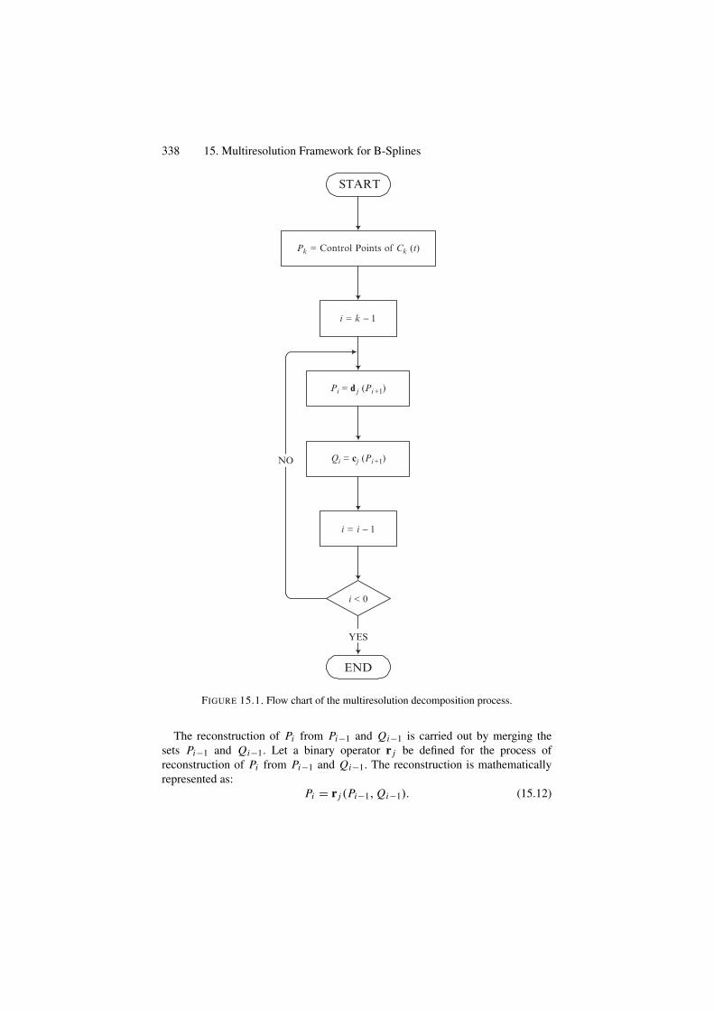
338 15. Multiresolution Framework for B-Splines
NO
Pk = Control Points of Ck (t)
i = k − 1
Pi = d j (Pi+1)
Qi = cj (Pi+1)
i = i − 1
i < 0
END
START
YES
FIGURE 15.1. Flow chart of the multiresolution decomposition process.
The reconstruction of Pi from Pi−1 and Qi−1 is carried out by merging thesets Pi−1 and Qi−1. Let a binary operator r j be defined for the process ofreconstruction of Pi from Pi−1 and Qi−1. The reconstruction is mathematicallyrepresented as:
Pi = r j (Pi−1, Qi−1). (15.12)
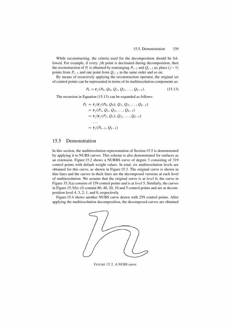
15.5. Demonstration 339
While reconstructing, the criteria used for the decomposition should be fol-lowed. For example, if every j th point is decimated during decomposition, thenthe reconstruction of Pi is obtained by rearranging Pi−1 and Qi−1 as; place ( j −1)points from Pi−1 and one point from Qi−1 in the same order and so on.
By means of recursively applying the reconstruction operator, the original setof control points can be represented in terms of its multiresolution components as:
Pk = r j (P0, Q0, Q1, Q2, . . . , Qk−1). (15.13)
The recursion in Equation (15.13) can be expanded as follows:
Pk = r j (r j (P0, Q0), Q1, Q2, . . . , Qk−1)
= r j (P1, Q1, Q2, . . . , Qk−1)
= r j (r j (P1, Q1), Q2, . . . , Qk−1)
. . .
= r j (Pk−1, Qk−1)
15.5 Demonstration
In this section, the multiresolution representation of Section 15.5 is demonstratedby applying it to NUBS curves. This scheme is also demonstrated for surfaces asan extension. Figure 15.2 shows a NURBS curve of degree 3 consisting of 319control points with default weight values. In total, six multiresolution levels areobtained for this curve, as shown in Figure 15.3. The original curve is shown inthin lines and the curves in thick lines are the decomposed versions at each levelof multiresolution. We assume that the original curve is at level 6; the curve inFigure 35.3(a) consists of 159 control points and is at level 5. Similarly, the curvesin Figure 15.3(b)–(f) contain 80, 40, 20, 10 and 5 control points and are at decom-position level 4, 3, 2, 1, and 0, respectively.
Figure 15.4 shows another NUBS curve drawn with 259 control points. Afterapplying the multiresolution decomposition, the decomposed curves are obtained
FIGURE 15.2. A NUBS curve.
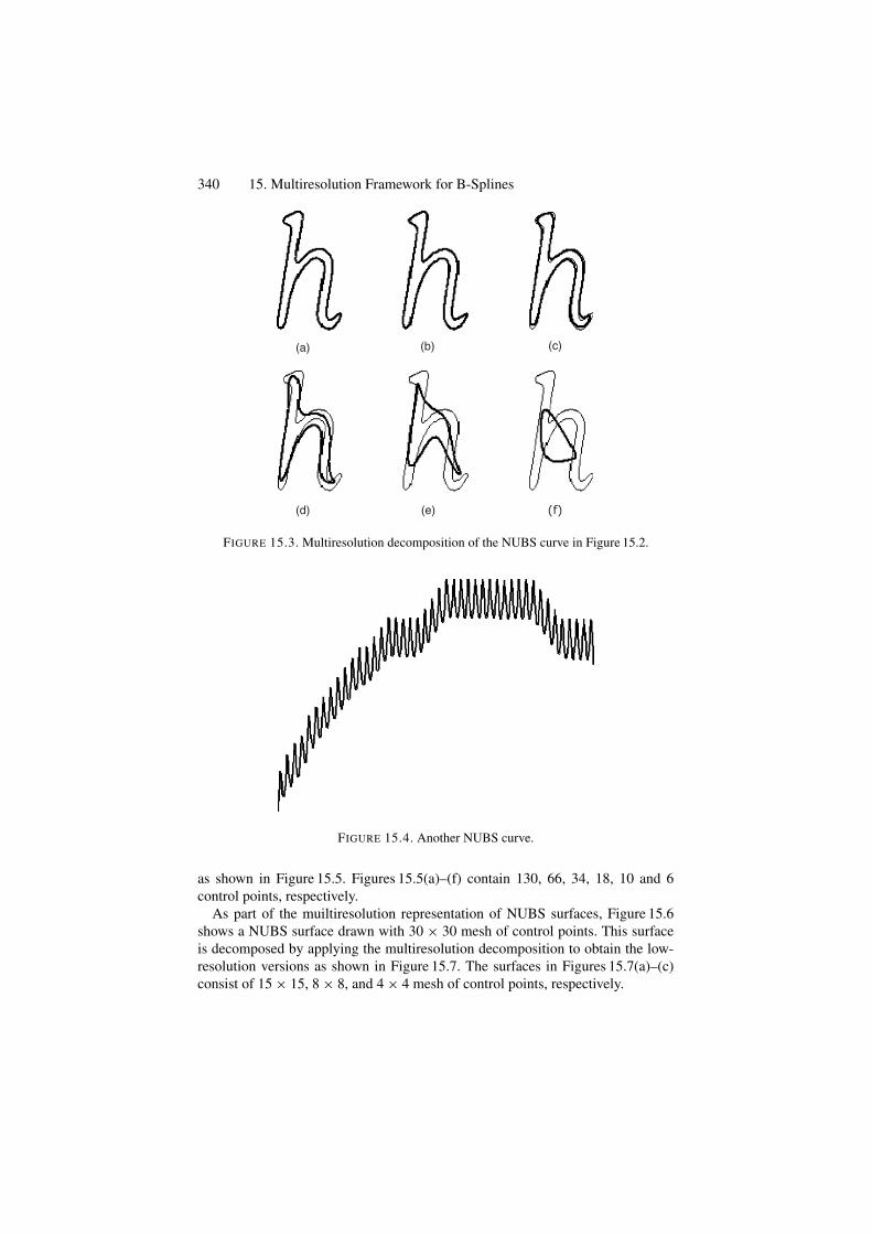
340 15. Multiresolution Framework for B-Splines
FIGURE 15.3. Multiresolution decomposition of the NUBS curve in Figure 15.2.
FIGURE 15.4. Another NUBS curve.
as shown in Figure 15.5. Figures 15.5(a)–(f) contain 130, 66, 34, 18, 10 and 6control points, respectively.
As part of the muiltiresolution representation of NUBS surfaces, Figure 15.6shows a NUBS surface drawn with 30 × 30 mesh of control points. This surfaceis decomposed by applying the multiresolution decomposition to obtain the low-resolution versions as shown in Figure 15.7. The surfaces in Figures 15.7(a)–(c)consist of 15 × 15, 8 × 8, and 4 × 4 mesh of control points, respectively.
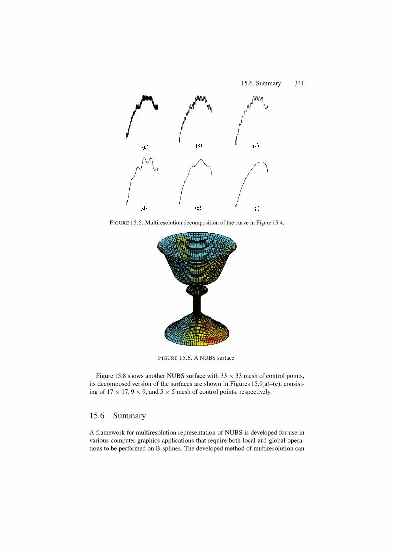
15.6. Summary 341
FIGURE 15.5. Multiresolution decomposition of the curve in Figure 15.4.
FIGURE 15.6. A NUBS surface.
Figure 15.8 shows another NUBS surface with 33 × 33 mesh of control points,its decomposed version of the surfaces are shown in Figures 15.9(a)–(c), consist-ing of 17 × 17, 9 × 9, and 5 × 5 mesh of control points, respectively.
15.6 Summary
A framework for multiresolution representation of NUBS is developed for use invarious computer graphics applications that require both local and global opera-tions to be performed on B-splines. The developed method of multiresolution can
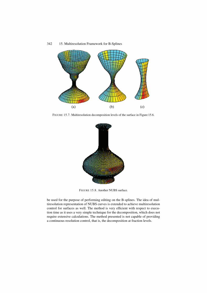
342 15. Multiresolution Framework for B-Splines
FIGURE 15.7. Multiresolution decomposition levels of the surface in Figure 15.6.
FIGURE 15.8. Another NUBS surface.
be used for the purpose of performing editing on the B-splines. The idea of mul-tiresolution representation of NUBS curves is extended to achieve multiresolutioncontrol for surfaces as well. The method is very efficient with respect to execu-tion time as it uses a very simple technique for the decomposition, which does notrequire extensive calculations. The method presented is not capable of providinga continuous resolution control, that is, the decomposition at fraction levels.
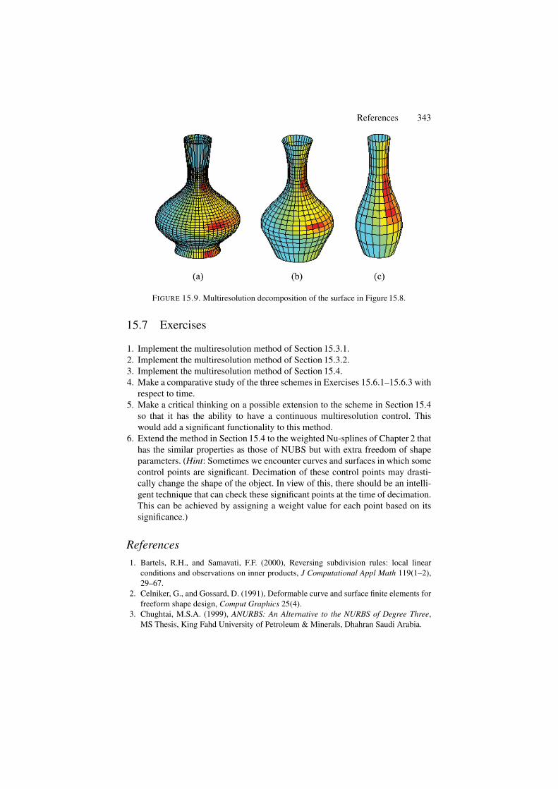
References 343
FIGURE 15.9. Multiresolution decomposition of the surface in Figure 15.8.
15.7 Exercises
1. Implement the multiresolution method of Section 15.3.1.2. Implement the multiresolution method of Section 15.3.2.3. Implement the multiresolution method of Section 15.4.4. Make a comparative study of the three schemes in Exercises 15.6.1–15.6.3 with
respect to time.5. Make a critical thinking on a possible extension to the scheme in Section 15.4
so that it has the ability to have a continuous multiresolution control. Thiswould add a significant functionality to this method.
6. Extend the method in Section 15.4 to the weighted Nu-splines of Chapter 2 thathas the similar properties as those of NUBS but with extra freedom of shapeparameters. (Hint: Sometimes we encounter curves and surfaces in which somecontrol points are significant. Decimation of these control points may drasti-cally change the shape of the object. In view of this, there should be an intelli-gent technique that can check these significant points at the time of decimation.This can be achieved by assigning a weight value for each point based on itssignificance.)
References1. Bartels, R.H., and Samavati, F.F. (2000), Reversing subdivision rules: local linear
conditions and observations on inner products, J Computational Appl Math 119(1–2),29–67.
2. Celniker, G., and Gossard, D. (1991), Deformable curve and surface finite elements forfreeform shape design, Comput Graphics 25(4).
3. Chughtai, M.S.A. (1999), ANURBS: An Alternative to the NURBS of Degree Three,MS Thesis, King Fahd University of Petroleum & Minerals, Dhahran Saudi Arabia.
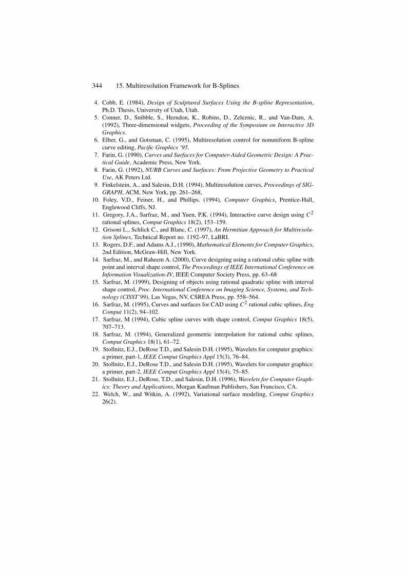
344 15. Multiresolution Framework for B-Splines
4. Cobb, E. (1984), Design of Sculptured Surfaces Using the B-spline Representation,Ph.D. Thesis, University of Utah, Utah.
5. Conner, D., Snibble, S., Herndon, K., Robins, D., Zeleznic, R., and Van-Dam, A.(1992), Three-dimensional widgets, Proceeding of the Symposium on Interactive 3DGraphics.
6. Elber, G., and Gotsman, C. (1995), Multiresolution control for nonuniform B-splinecurve editing, Pacific Graphics ’95.
7. Farin, G. (1990), Curves and Surfaces for Computer-Aided Geometric Design: A Prac-tical Guide, Academic Press, New York.
8. Farin, G. (1992), NURB Curves and Surfaces: From Projective Geometry to PracticalUse, AK Peters Ltd.
9. Finkelstein, A., and Salesin, D.H. (1994), Multiresolution curves, Proceedings of SIG-GRAPH, ACM, New York, pp. 261–268,
10. Foley, V.D., Feiner, H., and Phillips. (1994), Computer Graphics, Prentice-Hall,Englewood Cliffs, NJ.
11. Gregory, J.A., Sarfraz, M., and Yuen, P.K. (1994), Interactive curve design using C2
rational splines, Comput Graphics 18(2), 153–159.12. Grisoni L., Schlick C., and Blanc, C. (1997), An Hermitian Approach for Multiresolu-
tion Splines, Technical Report no. 1192–97, LaBRI.13. Rogers, D.F., and Adams A.J., (1990), Mathematical Elements for Computer Graphics,
2nd Edition, McGraw-Hill, New York.14. Sarfraz, M., and Raheem A. (2000), Curve designing using a rational cubic spline with
point and interval shape control, The Proceedings of IEEE International Conference onInformation Visualization-IV, IEEE Computer Society Press, pp. 63–68
15. Sarfraz, M. (1999), Designing of objects using rational quadratic spline with intervalshape control, Proc. International Conference on Imaging Science, Systems, and Tech-nology (CISST’99), Las Vegas, NV, CSREA Press, pp. 558–564.
16. Sarfraz, M. (1995), Curves and surfaces for CAD using C2 rational cubic splines, EngComput 11(2), 94–102.
17. Sarfraz, M (1994), Cubic spline curves with shape control, Comput Graphics 18(5),707–713.
18. Sarfraz, M. (1994), Generalized geometric interpolation for rational cubic splines,Comput Graphics 18(1), 61–72.
19. Stollnitz, E.J., DeRose T.D., and Salesin D.H. (1995), Wavelets for computer graphics:a primer, part-1, IEEE Comput Graphics Appl 15(3), 76–84.
20. Stollnitz, E.J., DeRose T.D., and Salesin D.H. (1995), Wavelets for computer graphics:a primer, part-2, IEEE Comput Graphics Appl 15(4), 75–85.
21. Stollnitz, E.J., DeRose, T.D., and Salesin, D.H. (1996), Wavelets for Computer Graph-ics: Theory and Applications, Morgan Kaufman Publishers, San Francisco, CA.
22. Welch, W., and Witkin, A. (1992), Variational surface modeling, Comput Graphics26(2).
Index
AAffine, 302Algebraic curve, 272Algorithm, 2, 4, 5, 15, 46, 50, 77,
133, 157, 173, 174, 179–181,190, 192, 193, 195, 196, 206,210–219, 221–223, 225–238,241–262, 267–270, 278, 283,284, 285, 293, 298, 299, 304,305, 306, 309, 312, 313, 316,319, 320, 322, 328, 329, 337
Analysis, 1–4, 29, 41–43, 46, 48, 56,64, 95, 99, 130, 135, 158, 175,185, 202, 209, 227, 237, 246,250, 261, 333–335
ANURBS, 343Approximation, 3–5, 41, 71, 124, 135,
142, 148, 153, 173Arc, 4, 56, 94–96, 102, 103, 105–109,
111, 195–197, 201–206, 210,246, 256
BBases, 22, 37, 42, 56Basis, 3, 4, 10, 11, 22, 23, 25–29, 31,
38, 55–57, 68, 76, 81–83,140, 192, 196, 230, 243, 256,282, 301, 303, 305, 306, 312,314, 316, 331–333, 335, 336
Bernstein, 11, 43, 45, 49, 56, 58–60, 62,63, 68–70, 76, 81, 84, 87, 97,99, 134, 196, 282
Bernstein-Bezier, 43, 45, 49, 56, 58–60,62, 63, 68–70, 76, 81, 84, 87,97, 99, 134, 282
Bezier, P., 1, 2, 5, 6, 11, 21–23, 30–32,37, 43–45, 49, 56, 58–60, 62,63, 68–70, 76, 81, 83, 84,87, 95, 97, 99, 105, 108, 109,134, 179, 195–197, 199, 203,236, 237, 267, 268, 272, 273,275, 276, 278, 279, 281, 282,287, 290, 293, 298, 331, 336
Bezier curve, 1, 13, 195, 267, 276, 293,298
Bezier patch, 70Bezier points, 69, 70, 105, 108Bezier spline, 11, 178, 179Blob, 244Boundary, 6, 197, 210, 223, 226, 227,
230, 236, 241, 242, 244, 245Boundary control points, 6, 332, 333Boundary points, 237, 246, 269, 270,
272–274, 299, 305, 313Biased, 2, 9, 10, 13, 41, 51, 55, 63, 78–
80, 88, 90, 91Biased tension, 9, 10, 63B-spline, 1–4, 10, 11, 21–23, 28, 38,
55–62, 64–68
CCAD, 2, 5, 21, 22, 41, 55, 75, 193, 297,
331CAGD, 2, 21, 38, 41, 55, 71, 94, 193,
331
345

346 Index
CAM, 2, 5, 21, 22, 41, 55, 75, 171,297
CARE system, 5, 297Cartesian, 4, 277Catmull-Rom spline, 12Close curve, 261, 282Closed curve, 12, 98, 226, 241, 244,
245, 247, 248, 261Compression, 246, 256Computer graphics, 1, 2, 4, 5, 21, 22,
38, 41, 71, 75Computer system, 267Continuity, 1, 3, 7–10, 13, 22, 23, 28,
45, 49Continuous, 7, 38, 87, 131, 181, 206,
293, 302, 342, 343Contour, 4, 5, 209, 219–221, 226–230,
241, 243, 249, 251Control, 1–3, 6, 8, 10, 11, 21–23, 31,
32, 34, 37Control point, 22, 56, 63, 85, 197, 204,
301, 304–306, 316, 332, 336,337
Control polygon, 10, 11, 31, 32, 34, 35,44, 59, 60, 62, 64
Convex, 3, 11, 21, 22, 43–45, 56, 76,97, 99, 108
Convex blob, 244Convex data, 119, 120, 124, 129, 131,
133, 148–150, 154, 158, 159Convex hull, 11, 21, 22, 43–45, 56, 76,
97, 99, 175, 302Convexity, 120, 122–126, 131, 133,
152–154, 157, 161, 162, 171,251
Convex set, 119, 150, 160Convex shape, 3, 117Convex spline, 148Corner cutting, 32, 60, 69, 84Corner point, 4, 5, 209–226, 228, 230Cubic interpolation, 125, 126, 131, 133,
157Curvature, 87, 99, 103, 104, 107, 119,
175, 195–197
Curve, 1–5, 7–12, 21–27, 31–35, 37Curve fitting, 267, 268, 272, 306, 309,
310, 312
DDatabase, 298Data point, 4, 37, 118, 133, 158, 164,
167, 173, 175, 176Data visualization, 21, 117, 129, 133De Boor point, 10Decimation, 332, 334–337, 343Decomposition, 6, 28, 50, 77, 98, 332–
343Default curve, 34, 100, 111, 112, 136,
137, 142, 148, 153, 154, 159,160, 309
Deformable, 343Degree, 2, 6, 10–13, 22, 42, 44, 45, 55,
94, 95Derivative, 3, 7, 9, 10, 12, 13, 23–27,
44, 45, 49, 76Design curve, 21–23, 31, 32, 42, 56, 58,
64, 69, 94, 99, 101, 137, 154,283
Digital, 4, 5, 209, 230, 242, 243, 251,259–261, 268, 293, 297
Digital curve, 4, 230, 242, 243, 251,259–261
Digitized, 279–281, 283, 298, 299, 303,306–309, 313, 317
Digitized curve, 279, 283Dimension, 31, 44, 59, 84, 107, 183Distance, 94, 97, 98, 100–102, 110,
178, 215, 216, 219Down-sampling, 334Dynamic programming, 242, 245, 246,
259–261
EEdge, 210, 259, 260, 269Editing, 331, 342Elliptic curve, 114Euclidean, 197, 245, 331Euclidean distance, 245, 331
Index 347
Euclidean norm, 197Evaluation, 2, 4, 6, 10, 37, 176, 182,
218, 221, 226, 230, 243, 256,257, 304, 305, 307, 314, 332
Evolutionary, 5, 297, 299, 328Evolutionary intelligence, 207, 330
FFilter, 250, 271, 334, 335Fitted curve, 268, 302, 305–307, 309,
314, 316, 318–320Fitting, 4, 5, 195, 204, 205, 243, 246,
251, 259–261, 267, 268, 272Freeform, 6, 21, 23, 28, 31, 38, 41, 42,
55, 56, 65, 75, 81
GGaussian filter, 250, 271, 293Geometric modeling, 4, 6, 21, 22, 38,
71, 130, 195, 206, 299, 314,331–333
Geometric surface, 330Global, 6, 32, 35, 36, 38, 46, 50–54, 62,
64, 66, 71, 75, 77Gray, 197, 201, 210, 229, 267Grid, 4, 161, 212
HHermite interpolation, 42, 96, 99Hierarchical, 263Hyperbolic curve, 114
IImage, 1, 4, 5, 93, 209, 210, 223, 227–
230, 236, 237, 267–269Image outline, 1Inflection, 102, 195Inflection point, 195Input, 174, 177, 179, 180, 184, 190,
211, 212, 230, 243, 246, 250,251
Interactive, 1, 3, 6, 38, 41, 71, 75, 113,136, 196, 267, 331, 336
Interface, 6, 196, 331
Interior, 97, 98, 183, 302, 333, 336Intermediate, 93–95, 109, 110, 114,
268, 273, 279, 294, 309, 316,323
Interpolate, 76, 110, 118, 193, 206, 273Interpolation, 3, 8, 24, 25, 26, 27, 37,
42, 44, 46, 50, 71, 78, 81, 84Intersection, 95, 101, 103, 106, 107,
176, 201Interval, 2, 3, 8, 9, 21–23, 25, 27–30,
33–35, 37, 38Interval tension, 2, 3, 21–23, 34, 35, 37,
41, 45, 50, 56, 62, 75, 77–79,85, 86, 90, 100, 110
Inverse relation, 335
KKnot, 6, 7, 10, 23, 29, 41, 47, 51, 54, 67,
76, 79, 118, 134Knot decimation, 334–336Knot insertion, 6, 177, 332Knot partition, 6, 7, 23, 29, 41Knot spacing, 174, 175, 333Knot value, 10, 174, 175, 314Knot vector, 6, 305, 307, 308, 314, 317,
332, 333, 335–337
LLevel of detail, 243Local, 3, 6, 22, 23, 28–35, 37, 38, 46,
51, 56, 57Loop, 219, 226, 261, 315
MMapping, 285, 288, 290–293, 304, 313Metropol, 317Metropolis, 315, 316Model curve, 131Monotone, 117, 145, 147, 157–159,
162–164, 195, 200, 201, 206Multi-resolution, 6, 332–343Multi-resolution analysis, 333, 334Multi-resolution curve, 18, 344Multi-resolution decomposition, 6, 332,
333, 335–343
348 Index
Multi-resolution framework, 6, 331–342
Multi-resolution spline, 19, 344
NNeighborhood, 94, 111, 134, 210, 246,
306, 313, 316Noise, 160, 162, 183, 185, 210, 211,
218, 221, 223, 226–231, 235,251, 268, 271, 272
Nu spline, 1, 2, 3, 8–10, 22, 26–28, 34–36, 38, 78, 86
NUBS curve, 303, 335–337, 339, 340,342
NUBS surface, 340–342NURBS curve, 298, 301–303, 305, 308,
309, 312, 315, 316, 339NURBS surface, 322–324, 326, 327NURBS, 1, 5, 56, 64–71, 94, 195, 297–
299, 301–303, 305–312
OObject recognition, 209Open curve, 12, 97, 245, 282, 333Optimal, 5, 181, 193, 237, 242, 243,
245, 251, 259–261, 274, 283,298
Optimal curve, 298Optimization, 173, 179, 181, 259, 260,
298, 299, 304, 306–309, 312–317, 321–323
Order, 1, 8–10, 28, 51, 178, 183, 185,199, 210, 261, 269, 272, 294,301–303, 305, 309, 313, 314,316, 321, 322, 326, 333, 335–337, 339
Orientation, 290Outline, 5, 93, 181, 182, 205, 210, 227,
236, 237, 267, 270, 271, 279Output, 5, 98, 142, 148, 185, 210, 245,
299, 305, 337
PParabolic, 94, 95, 102–104Parabolic curve, 114
Parameter, 3, 10, 12, 13, 28, 34, 41, 42,44, 49, 51, 79, 80, 81, 85, 87–89, 96, 100, 106
Parametric continuity, 56Parametric curve, 9, 10, 26, 27, 41, 93,
124, 173, 267, 274, 276, 277,279
Parametric surface, 288, 289Partition of unity, 22, 31, 55, 57, 82, 83Patch, 70, 323Path, 4, 195, 205, 206, 259Pattern recognition, 209Performance evaluation, 218, 221, 230Piecewise, 3, 4, 7–10, 21–27, 31, 32,
42, 46Planar, 4, 5, 43, 118, 195, 284, 288, 299,
302, 313Planar curve, 43, 118, 195Planar data, 16, 206Planar image, 4, 5, 313Planar object, 5, 299Planar shapes, 5Planar surface, 288Plane, 3, 31, 44, 59, 84, 101, 106, 117,
124, 199, 200, 201, 246, 290,300, 302
Point, 2–5, 8–10, 21–23, 26–28, 35, 37,38
Point decimation, 332, 336, 337Point tension, 9, 10, 23, 26–28, 34, 35,
51, 54, 63, 67, 75, 77–79, 86,90, 111
Polygonal approximation, 5, 230, 241–246, 250–252, 256, 259, 261,262
Polygonal curve, 264, 265Polynomial, 2, 8, 11, 60, 61, 133, 134,
140, 157, 158, 162Positive interpolation, 140, 164, 167Prefiltering, 295Projection, 2Pseudo-code, 252, 253
Index 349
QQuadratic interpolation, 131Quadratic spline, 94, 133Quintic, 277
RRational cubic, 41–46, 49–51, 56, 58,
64, 70, 71, 75Rational curve, 2, 44, 76Rational interpolation, 117–126Rational polynomial, 301Rational quadratic, 94, 133, 196, 197Rational spline, 3, 41, 42, 46, 48–55, 57Ray, B.K., 250, 251, 254–256Ray, K.S., 250, 251, 254–256Recognition, 5, 209, 241Rectangular, 38, 234Recursive formula, 332Recursive function, 10, 253, 260Recursive method, 37, 242Recursive relation, 14, 39, 72, 92Refinement, 178, 306, 314Region, 11, 69, 71, 113, 140, 153, 197,
200, 201, 210, 242–244, 249,250
Resolution, 6, 177, 211, 221, 229, 230,269, 333, 334, 336, 337, 342
Reverse engineering, 5, 297, 312, 328Robust, 21, 173, 179, 209, 219, 231,
251, 328
SSample data, 271Scalar, 3, 7, 43, 117, 122, 124, 133Sculptured surface, 344Segment, 32, 33, 44, 46, 62, 76, 103,
107, 110Segmentation, 4, 209, 236, 237, 242,
268Shape control, 2, 3, 8, 21–23, 32–34,
41, 71, 77, 78, 84, 85, 106,112, 133–135, 158
Shape parameter, 3, 21, 22, 28, 32, 37,38, 41, 42, 49, 50, 54, 56, 71,78, 80, 85, 100, 137, 149
Shape preservation, 126, 131, 154, 171Shape recognition, 5, 241Simulated annealing, 5, 298, 299, 312,
313, 316, 328, 329Simulation, 16, 128, 156Smooth curve, 129, 205, 306Solid line, 205, 275, 276, 279Space, 6, 22, 94, 95, 107, 113, 181, 288,
290, 292, 293, 305, 335–337Space curve, 94, 95, 113, 114Span, 10, 333Spiral, 195–206Spiral interpolation, 205Spline, 2, 3, 7–13, 22–28, 38Spline curve, 7, 10, 12, 21, 33, 38, 48,
113, 129, 142, 160, 183, 283Spline interpolation, 3, 46, 50, 78, 133,
139–142, 148–153Spline surface, 37, 70Subdivision2, 236, 343Subspace, 335, 336Surface approximation, 5, 297, 298Surface design, 3, 38, 71, 94Surface editing, 1Surface fairing, 4, 195, 206Surface mapping, 290–293Surface, 2, 4, 6, 37, 38, 42, 70, 71, 95,
113, 195, 199, 288–293System, 5, 6, 22, 24–28, 45–51, 77, 98,
196, 210, 271, 303, 332
TTension, 8–10, 12, 13, 21–23, 26, 28,
34, 35, 38, 41Threshold, 173, 176, 178, 214, 215,
229, 256, 258, 279Time complexity, 261Typeface, 17, 294
VVariation diminishing, 22, 23, 32, 44,
56, 60, 69, 84, 97, 99, 100,302
Variational surface, 344Vertex, 64, 287

350 Index
Vertices, 28, 30, 60, 97, 199, 245, 251,259–261, 337
Visualization, 4, 21, 129–154Volume, 166
WWavelets, 246, 332–335
Weight, 28, 43, 96, 183, 197, 298, 305–307, 309, 313–317, 323, 339
Weighted Nu spline, 2, 9, 22, 28–36, 78,86
Weighted spline, 8–10, 24, 25, 27, 78,85
Recommended