MARC-ANDRÉ CARLE
LA MÉTAHEURISTIQUE CAT POUR LE DESIGN DE RÉSEAUX LOGISTIQUES DÉTERMINISTES ET
STOCHASTIQUES
Thèse présentée à la Faculté des études supérieures et postdoctorales de l'Université Laval
dans le cadre du programme de doctorat en sciences de l'administration pour l'obtention du grade de Philosophiae Doctor (Ph.D.)
DÉPARTEMENT OPÉRATIONS ET SYSTÈMES DE DÉCISION
FACULTE DES SCIENCES DE L'ADMINISTRATION UNIVERSITÉ LAVAL
QUÉBEC
2012
©Marc-André Carle, 2012

ii
Résumé
De nos jours, les entreprises d’ici et d’ailleurs sont confrontées à une concurrence mondiale sans
cesse plus féroce. Afin de survivre et de développer des avantages concurrentiels, elles doivent
s’approvisionner et vendre leurs produits sur les marchés mondiaux. Elles doivent aussi offrir
simultanément à leurs clients des produits d’excellente qualité à prix concurrentiels et assortis
d’un service impeccable. Ainsi, les activités d’approvisionnement, de production et de marketing
ne peuvent plus être planifiées et gérées indépendamment.
Dans ce contexte, les grandes entreprises manufacturières se doivent de réorganiser et
reconfigurer sans cesse leur réseau logistique pour faire face aux pressions financières et
environnementales ainsi qu’aux exigences de leurs clients. Tout doit être révisé et planifié de
façon intégrée : sélection des fournisseurs, choix d’investissements, planification du transport et
préparation d’une proposition de valeur incluant souvent produits et services au fournisseur. Au
niveau stratégique, ce problème est fréquemment désigné par le vocable « design de réseau
logistique ».
Une approche intéressante pour résoudre ces problématiques décisionnelles complexes consiste à
formuler et résoudre un modèle mathématique en nombres entiers représentant la problématique.
Plusieurs modèles ont ainsi été récemment proposés pour traiter différentes catégories de décision
en matière de design de réseau logistique. Cependant, ces modèles sont très complexes et
difficiles à résoudre, et même les solveurs les plus performants échouent parfois à fournir une
solution de qualité.
Les travaux développés dans cette thèse proposent plusieurs contributions. Tout d’abord, un
modèle de design de réseau logistique incorporant plusieurs innovations proposées récemment
dans la littérature a été développé; celui-ci intègre les dimensions du choix des fournisseurs, la
localisation, la configuration et l’assignation de mission aux installations (usines, entrepôts, etc.)
de l’entreprise, la planification stratégique du transport et la sélection de politiques de marketing
et d’offre de valeur au consommateur. Des innovations sont proposées au niveau de la
modélisation des inventaires ainsi que de la sélection des options de transport.

iii
En deuxième lieu, une méthode de résolution distribuée inspirée du paradigme des systèmes
multi-agents a été développée afin de résoudre des problèmes d’optimisation de grande taille
incorporant plusieurs catégories de décisions. Cette approche, appelée CAT (pour collaborative
agent teams), consiste à diviser le problème en un ensemble de sous-problèmes, et assigner
chacun de ces sous-problèmes à un agent qui devra le résoudre. Par la suite, les solutions à
chacun de ces sous-problèmes sont combinées par d’autres agents afin d’obtenir une solution de
qualité au problème initial. Des mécanismes efficaces sont conçus pour la division du problème,
pour la résolution des sous-problèmes et pour l’intégration des solutions.
L’approche CAT ainsi développée est utilisée pour résoudre le problème de design de réseaux
logistiques en univers certain (déterministe). Finalement, des adaptations sont proposées à CAT
permettant de résoudre des problèmes de design de réseaux logistiques en univers incertain
(stochastique).
4
Table des matières
RÉS UMÉ .......................................................................................................................................................................................... II
TABLE DES MATIÈRES ............................................................................................................................................................4
REMERCIEMENTS ......................................................................................................................................................................9
AVANT-PROPOS........................................................................................................................................................................ 11
LISTE DES FIGURES ............................................................................................................................................................... 13
LISTE DES TABLEAUX .......................................................................................................................................................... 14
1 INTRODUCTION.............................................................................................................................................................. 15
1.1 CHAÎNE LOGISTIQUE ET DESIGN DE RÉSEAU LOGISTIQUE....................................................................................... 15
1.2 TERMINOLOGIE ET CONCEPTS CLÉS ........................................................................................................................... 18
1.2.1 Problème de décision ............................................................................................................................................ 18
1.2.2 Modélisation mathématique ................................................................................................................................. 20
1.2.3 Algorithme d’optimisation.................................................................................................................................... 21
1.2.4 Interrelations entre problématique, modèle et algorithme ............................................................................. 21
1.3 QUE PEUT -ON ESPÉRER DE L’AIDE À LA DÉCISION EN CONTEXTE DE DESIGN DE RÉSEAU LOGISTIQUE ?......... 22
1.3.1 Du rôle et des objectifs de la méthodologie ...................................................................................................... 23
1.3.2 Des bénéfices engendrés par l’aide à la décision en contexte de design de réseau logistique ................ 24
1.3.3 Des apports de l’aide à la décision en contexte de design de réseau logistique ........................................ 25
1.4 OBJECTIFS ET STRUCTURE DE LA THÈSE ................................................................................................................... 26
2 THE DES IGN OF S UPPLY CHAIN NETWORKS ................................................................................................. 28
2.1 DISTRIBUTED DECISION MAKING AND SCN DESIGN ............................................................................................... 28
2.2 CHARACTERISTICS OF SCN DESIGN MODELS ........................................................................................................... 30
2.2.1 Organizational context.......................................................................................................................................... 31
2.2.1.1 Wholly-owned supply chains .................................................................................................................................. 31
2.2.1.2 Multi-division enterprises ........................................................................................................................................ 32
2.2.1.3 Multi-firm supply chains ......................................................................................................................................... 32
2.2.2 Evaluation of the supply chain performances................................................................................................... 33
5
2.2.2.1 Mono-objective models ........................................................................................................................................... 34
2.2.2.2 Multi-objective models ............................................................................................................................................ 35
2.2.3 Modeling of tactical and operational decisions ............................................................................................... 37
2.2.4 Temporal representations..................................................................................................................................... 38
2.2.5 Uncertainty and risk modeling ............................................................................................................................ 39
2.2.6 Modeling activities, processes and products .................................................................................................... 41
2.2.7 SCN representation ............................................................................................................................................... 41
2.2.7.1 Multi-echelon networks ........................................................................................................................................... 42
2.2.7.2 General supply chain network ................................................................................................................................. 43
2.2.8 Modeling markets, demand, price and service ................................................................................................. 44
2.2.9 Modeling facilities and capacity options ........................................................................................................... 46
2.2.10 Modeling product flows and inventories....................................................................................................... 47
2.2.11 Cost modeling .................................................................................................................................................... 48
2.2.12 Emerging trends ................................................................................................................................................ 49
2.3 OUTSTANDING ISSUES AND SHORTCOMINGS OF THE CURRENT LITERATURE ...................................................... 49
3 OPTIMIZATION ALGORITHMS US ED TO SOLVE SCN DES IGN MODELS .......................................... 52
3.1 EXACT APPROACHES .................................................................................................................................................... 52
3.1.1 Branch-and-bound................................................................................................................................................. 52
3.1.2 Cutting Plane Algorithms and Branch-and-cut ................................................................................................ 53
3.1.2.1 Commercial branch-and-cut based solvers .............................................................................................................. 54
3.1.3 Lagrangian relaxation .......................................................................................................................................... 55
3.1.4 Primal decomposition techniques ....................................................................................................................... 56
3.1.5 Other exact approaches ........................................................................................................................................ 57
3.2 HEURISTICS ................................................................................................................................................................... 57
3.2.1 Classical heuristics................................................................................................................................................ 58
3.2.2 Metaheuristics ........................................................................................................................................................ 59
3.2.2.1 Single-solution based metaheuristics....................................................................................................................... 59
3.2.2.2 Population-based metaheuristics...................................................................................................................... 62
3.2.3 Heuristics based on mathematical programming ............................................................................................ 64
3.3 HYBRID ALGORITHMS .................................................................................................................................................. 66
3.3.1 Hybrid metaheuristics ........................................................................................................................................... 66
6
3.3.2 Hybrids between exact methods and metaheuristics ....................................................................................... 66
3.3.3 Agent-based algorithms ........................................................................................................................................ 67
3.4 ALGORITHMS AND APPROACHES FOR SOLVING STOCHASTIC MODELS ................................................................. 69
3.4.1 Sample Average Approximation (SAA) methods .............................................................................................. 69
3.4.2 Integer L-Shaped Method ..................................................................................................................................... 69
3.4.3 Progressive Hedging ............................................................................................................................................. 70
3.4.4 Other approaches .................................................................................................................................................. 70
3.5 CRITICAL REVIEW OF EXISTING APPROACHES .......................................................................................................... 71
4 L’APPROCHE CAT POUR L’OPTIMISATION DISTRIBUÉE DE PROBLÈMES
MULTIDIMENS IONNELS ...................................................................................................................................................... 73
4.1 RÉSUMÉ DE L’ARTICLE ................................................................................................................................................ 73
4.2 COLLABORATIVE AGENT TEAMS (CAT) FOR DISTRIBUTED MULTIDIMENSIONAL OPTIMIZATION ................... 73
4.2.1 Abstract.................................................................................................................................................................... 74
4.2.2 Introduction ............................................................................................................................................................ 74
4.2.3 Strategies to tackle complex problems/models ................................................................................................. 76
4.2.4 CAT as an agent-based metaheuristic................................................................................................................ 80
4.2.5 Experimental test case .......................................................................................................................................... 94
4.2.5.1 Multi-Period Supply Chain Network Design Model ............................................................................................... 94
4.2.5.2 CAT Implementation ............................................................................................................................................... 96
4.2.6 Computational results ......................................................................................................................................... 101
4.2.7 Conclusion ............................................................................................................................................................ 105
4.2.8 References ............................................................................................................................................................. 106
5 UNE APPROCHE CAT POUR LA RÉSOLUTION DE PROBLÈME DE DESIGN DE RÉSEAUX
LOGIS TIQUES DÉTERMINIS TES MULTI-PÉRIODES BAS ÉS S UR LES ACTIVITÉS ............................... 111
5.1 RÉSUMÉ DE L’ARTICLE .............................................................................................................................................. 111
5.2 THE CAT METAHEURISTIC FOR THE SOLUTION OF MULTI-PERIOD ACTIVITY-BASED SUPPLY CHAIN
NETWORK DESIGN PROBLEMS ................................................................................................................................................ 111
5.2.1 Abstract.................................................................................................................................................................. 112
5.2.2 Introduction .......................................................................................................................................................... 112
5.2.3 Literature Review................................................................................................................................................. 113
5.2.4 Activity-Based View of the Supply Chain Network Design Problem .......................................................... 116
7
5.2.4.1 Planning Horizon and Time Representation.......................................................................................................... 116
5.2.4.2 Products, Activities and Locations ........................................................................................................................ 117
5.2.4.3 Transportation Options .......................................................................................................................................... 119
5.2.4.4 Platforms................................................................................................................................................................ 120
5.2.4.5 Vendor Contracts ................................................................................................................................................... 123
5.2.4.6 Product-Markets and Marketing Policies .............................................................................................................. 123
5.2.4.7 Supply Chain Network .......................................................................................................................................... 125
5.2.4.8 Order Cycle and Safety Stocks .............................................................................................................................. 129
5.2.5 Mathematical Programming Model ................................................................................................................. 131
5.2.6 Solution Approach ............................................................................................................................................... 134
5.2.7 Computational Results ........................................................................................................................................ 138
5.2.8 Conclusions........................................................................................................................................................... 142
5.2.9 References ............................................................................................................................................................. 143
6 DESIGN DE RÉSEAUX LOGISTIQUES EN CONTEXTE STOCHASTIQUE MULTI-PÉRIODES
MULTI-ACTIVITÉS ................................................................................................................................................................ 149
6.1 RÉSUMÉ DE L’ARTICLE .............................................................................................................................................. 149
6.2 A CAT METAHEURISTIC FOR THE SOLUTION OF STOCHASTIC SUPPLY CHAIN NETWORK DESIGN PROBLEMS
149
6.2.1 Abstract.................................................................................................................................................................. 149
6.2.2 Introduction .......................................................................................................................................................... 150
6.2.3 Supply Chain Modeling ...................................................................................................................................... 151
6.2.3.1 Supply Chain Modeling Approach ........................................................................................................................ 151
6.2.3.2 Modeling Randomness .......................................................................................................................................... 153
6.2.3.3 SCN Design Model................................................................................................................................................ 154
6.2.4 Solution Approach ............................................................................................................................................... 158
6.2.4.1 CAT Structure and Sub-Models ............................................................................................................................ 158
6.2.4.2 Solving Stochastic SCN Design Problems with CAT ........................................................................................... 160
6.2.4.3 Agents and Algorithms .......................................................................................................................................... 160
6.2.5 Computational Results ........................................................................................................................................ 166
6.2.5.1 Comparisons with CPLEX’s SAA Solutions ........................................................................................................ 167
6.2.5.2 Taking Nonlinearities into Account....................................................................................................................... 170
8
6.2.5.3 Results for Risk-Averse Models ............................................................................................................................ 170
6.2.6 Conclusion ............................................................................................................................................................ 172
6.2.7 References ............................................................................................................................................................. 173
7 CONCLUS ION ................................................................................................................................................................. 176
7.1 CONTRIBUTIONS PRINCIPALES DE LA THÈSE .......................................................................................................... 177
7.1.1 CAT, une métaheuristique basée sur le paradigme agents........................................................................... 177
7.1.2 Un modèle générique de design de réseaux logistiques basé sur les activités en contexte déterministe
178
7.1.3 Un modèle générique de design de réseaux logistiques basé sur les activités en contexte stochastique
179
7.2 EXTENSIONS ET TRAVAUX FUTURS.......................................................................................................................... 179
7.2.1 Design de réseaux logistiques ........................................................................................................................... 179
7.2.2 CAT......................................................................................................................................................................... 180
7.2.2.1 Applications de CAT pour la decision distribuée.................................................................................................. 180
7.2.2.2 Librairie générique pour CAT ............................................................................................................................... 181
7.2.2.3 Paramétrage et auto-paramétrage des agents ......................................................................................................... 182
8 RÉFÉRENCES GÉNÉRALES ..................................................................................................................................... 184

9
Remerciements
Les travaux conduisant à la présentation de cette thèse ont été réalisés sous la supervision et avec
le soutien et le support de mon directeur de recherche, M. Alain Martel, ainsi que de mon co-
directeur, M. Nicolas Zufferey. Chacun d’eux a été à sa façon d’une aide précieuse, et sans leur
soutien cet aboutissement n’aurait pas été possible. Je tiens donc à les remercier tout
particulièrement. M. Martel a su, par son souci de rigueur, me convaincre de pousser plus loin
l’analyse afin d’arriver à des contributions plus générales et surtout plus solides sur le plan
méthodologique. Je salue également sa détermination à s’assurer de la qualité de nos
communications écrites et pour son soutien logistique et financer afin que je puisse participer à
des conférences. Je remercie Nicolas Zufferey pour son pragmatisme et sa disponibilité malgré
l’océan Atlantique qui nous sépare plus de 10 mois par année. Il m’a également enseigné une
leçon que je n’ai pas fini d’intégrer : rechercher l’efficacité dans la simplicité plutôt que dans la
complexité.
Mes prochains remerciements vont aux professeurs du département OSD avec qui j’ai eu
l’occasion de travailler au cours des années. Merci à Irène Abi-Zeid et à Benoît Montreuil pour
m’avoir fait découvrir différents paradigmes et approches; cela m’a permis d’avoir davantage de
recul par rapport à mes travaux et davantage de modestie par rapport aux résultats que je puis
compter obtenir. Merci à Monia Rekik pour sa révision rigoureuse de mes travaux préliminaires
et pour ses critiques, parfois sévères, mais toujours constructives. Merci à Jacques Renaud et
Angel Ruiz, mes mentors de maîtrise, qui ont su me donner le goût de la recherche assez tôt dans
mon cheminement académique et qui m’ont supporté dans mes études préalables.
Je remercie également les employés du CIRRELT avec qui j’ai eu le plaisir de travailler :
Stéphane Caron et Olivier Duval-Montminy pour le réseau du CIRRELT qui fonctionne, ainsi
que Louise Doyon, Mireille Leclerc et Pierre Marchand pour leur disponibilité et les nombreux
services qu’ils m’ont rendus au cours des années.
Je salue également mes compagnons de toujours au département, Joëlle Bouchard, Marie-Claude
Bolduc, Walid Klibi (maintenant à Bordeaux), Sylvain Girard et plus récemment Michael Morin.
Votre soutien m’a été précieux.

10
Ceux qui me connaissent savent que je ne suis pas très bavard sur ma vie personnelle. Une
reconnaissance toute particulière va à ma famille, mes parents, leurs conjoints et mes sœurs, pour
leur soutien indéfectible au cours des années d’étude. Un merci particulier à Magalie pour sa
patience et ses encouragements lors de moments difficiles qui surviennent inévitablement dans le
cadre d’un projet aussi long. Sans votre soutien, j’aurais peut-être débuté ce projet, mais je ne
l’aurais certainement pas terminé. Mille mercis.

11
Avant-propos
Le présent document constitue la thèse que j’ai réalisée dans le cadre de mes études doctorales à
l’Université Laval, sous la direction du professeur Alain Martel et la codirection du professeur
Nicolas Zufferey. Les travaux de recherche ont été réalisés au CIRRELT (Centre
interuniversitaire de recherche sur les réseaux d’entreprise, la logistique et le transport), dans le
cadre du projet DRESNET (Design of Robust and Effective Supply Networks). Ce projet a
notamment financé une grande partie de mes travaux de recherche.
Cette thèse par articles est constituée d’une introduction, suivie de deux chapitres de revue de
littérature, couvrant respectivement le design de réseaux logistiques et les méthodes de résolution
de modèles d’optimisation en nombres entiers. Ceux-ci sont suivis de trois articles acceptés ou
soumis pour publication. Pour chacun de ces articles, j’ai agi à titre de chercheur principal : j’ai
contribué au développement des concepts et des modèles mathématiques, conçu et programmé
l’ensemble des algorithmes d’optimisation et du système multi-agents, préparé et réalisé les
expérimentations et travaillé à la rédaction des articles.
Le premier article intitulé « Collaborative Agent Teams (CAT) for distributed multi-dimensional
optimization » et inséré au chapitre 4, présente CAT, l’approche générale de modélisation et de
résolution de problèmes, basée sur le paradigme multi-agents, qui a été élaborée dans le cadre de
ma thèse. Il a été écrit en collaboration avec les professeurs Alain Martel et Nicolas Zufferey. Il a
été soumis pour publication à la revue Computers and Operations Research. La version présentée
dans ce document est celle soumise à la revue.
Le deuxième article, inséré au chapitre 5, est intitulé « The CAT Metaheuristic for the Solution of
Multi-Period Activity-Based Supply Chain Network Design Problems ». Il présente un modèle
générique d’optimisation pour une classe de problèmes de design de réseaux logistiques en
contexte déterministe, et il montre comment le résoudre avec la métaheuristique CAT. Une
version modifiée de ce modèle a été implantée dans le logiciel SC Studio, partiellement
développé dans le cadre du projet DRESNET. Cet article a été publié dans la revue International
Journal of Production Economics, aux pages 664 à 677 du volume 139. La version présentée
dans ce document correspond à la version publiée.

12
Le troisième article, inséré au chapitre 6, est intitulé « A CAT Metaheuristic for the Solution of
Stochastic Supply Chain Network Design Problems ». Il présente une approche permettant
d’intégrer l’incertitude associée aux paramètres économiques au sein de modèles d’optimisation
du design des réseaux logistiques, et il montre comment résoudre ces problèmes avec CAT. Cet
article sera soumis sous peu à la revue European Journal of Operational Research.
13
Liste des figures
Figure 1: Trois volets de la recherche en design de réseau logistique ........................................... 22
Figure 2: Performance evaluation methods for mono-objective models ....................................... 35
Figure 3: Multi-echelon network. Taken from (Martel, 2005) ...................................................... 42
Figure 4: CAT Problem Solving Constructs .................................................................................. 82
Figure 5: A Linking Integration Sub-Model................................................................................... 85
Figure 6: A Merging Integration Sub-Model ................................................................................. 86
Figure 7: Main Components of a CAT System.............................................................................. 87
Figure 8: Sample Solution Digraph................................................................................................ 93
Figure 9: CAT Constructs for the Multi-Period SCN Design Problem ......................................... 97
Figure 10: Planning Periods ......................................................................................................... 117
Figure 11: Directed Activity Graph Example from the Lumber Industry.................................... 118
Figure 12: Supply Chain Network Representation for a Time Period ......................................... 126
Figure 13: CAT Components ....................................................................................................... 135
14
Liste des tableaux
Tableau 1: Questions associées au design de réseaux logistique ................................................... 17
Tableau 2: Exemples de problématiques décisionnelles ................................................................ 19
Tableau 3: Lien entre les objectifs de la thèse et les articles .......................................................... 27
Table 4: Propagation Index Updates .............................................................................................. 93
Table 5: Sub-Models Associated with the Resource-Based View ................................................. 98
Table 6: Time-Based Partitioning ................................................................................................ 100
Table 7: CAT Agents Implemented to Solve the SCN Design Problem ..................................... 101
Table 8: Agents Included in each Version of CAT ...................................................................... 103
Table 9: Computational Results after 60 Minutes........................................................................ 104
Table 10: Computational Results after 10 Hours (600 Minutes) ................................................. 105
Table 11: Network Expenses ........................................................................................................ 131
Table 12: Site Revenues and Expenses ........................................................................................ 132
Table 13: CAT Agents Implemented............................................................................................. 137
Table 14: Performance obtained for a 1-hour time limit for CAT and CPLEX.......................... 140
Table 15: Performance obtained for an 8 hour time limit for CAT and CPLEX ......................... 141
Table 16: Performance for different problem classes .................................................................. 142
15
1 Introduction
De nos jours, les entreprises d’ici et d’ailleurs sont confrontées à une concurrence
mondiale sans cesse plus féroce. Afin de survivre et de développer des avantages concurrentiels,
elles doivent s’approvisionner et vendre leurs produits sur les marchés mondiaux tout en offrant
simultanément à leurs clients des produits d’excellente qualité à prix concurrentiels et assortis
d’un service impeccable. Selon Martel (2003b), pour demeurer compétitive, « une entreprise doit
continuellement réussir à remporter des commandes sur ses marchés mieux que ses
compétiteurs ». Dans ce contexte, les décisions associées à la conception et à la gestion de la
chaîne logistique ont des impacts importants sur des facteurs clés tels que la qualité des produits,
le délai de livraison offert aux clients ainsi que le coût total de production et de distribution de
chaque produit. Ces décisions étant toutefois complexes et inter-reliées, J. F. Shapiro (2007)
souligne l’apport considérable que peuvent apporter les domaines de l’analyse de données, de la
modélisation et de l’optimisation dans la compréhension et la résolution de ces problèmes
décisionnels.
Cette introduction est divisée en quatre sections. La section 1.1 positionne le design de
réseaux logistiques dans le contexte de planification des activités logistiques d’une entreprise. La
section 1.2 présente brièvement le domaine de recherche et précise la terminologie utilisée dans
l’ensemble de la thèse. La section 1.3 illustre brièvement les trois types de bénéfices directs et
indirects associés à l’application du type de recherche proposée dans cette thèse au sein
d’entreprises manufacturières. Finalement, la section 1.4 décrit les objectifs de la thèse ainsi que
sa structure.
1.1 Chaîne logistique et design de réseau logistique
Cette section brosse un portrait général et agrégé du domaine de recherche. Le lecteur
intéressé par une analyse plus spécifique des principales publications et approches se rapportant à
notre domaine de recherche se référera plutôt aux chapitres 2 et 3 de la thèse. On utilise
généralement le vocable de chaîne logistique (Oliver & Webber, 1992) ou chaîne de valeur
(Porter, 1985) pour définir l’ensemble des processus et des activités par lesquels une entreprise
ou un ensemble d’entreprises crée ou génère de la valeur, généralement sous la forme de produits
et services conçus, fabriqués, distribués et habituellement vendus ou offerts à un ensemble de
clients ou bénéficiaires. Au sein d’une chaîne logistique, une entreprise peut intervenir au sein de

16
la totalité ou d’un sous-ensemble des processus. De nos jours, le rôle crucial joué par l’ensemble
des activités associées à la chaîne logistique dans la compétitivité d’une entreprise constitue un
paradigme dominant.
Ceci étant dit, l’atteinte de l’excellence en matière de gestion de la chaîne logistique
s’avère une tâche très complexe, comme le fait remarquer Stadtler (2008). L’un des facteurs
expliquant cette complexité s’avère la quantité et la variété des décisions à prendre
simultanément dans le cadre de la gestion de la chaîne logistique. Qui plus est, ces décisions sont
souvent prises par une myriade d’acteurs aux fonctions et aux responsabilités différentes. Le
Supply Chain Council identifie cinq défis principaux pour les chaînes logistiques modernes : un
service à la clientèle exemplaire, le contrôle des coûts, la planification et la gestion du risque, la
gestion des partenariats (tant avec les clients qu’avec les fournisseurs) et la capacité à développer
les compétences du personnel (2012). Dans la gestion de la chaîne logistique, nous nous
intéressons tout particulièrement aux activités se rapportant à la planification. Selon Fleischmann,
Meyr, and Wagner (2008), les décisions associées à la planification de la chaîne logistique
diffèrent également par leur ampleur et leur portée (dans le temps et l’espace). Les mêmes
auteurs distinguent d’une part, la planification associée aux décisions opérationnelles, qui vise à
produire des instructions détaillées pour les opérations courantes; ces décisions ont une portée à
court terme, et d’autre part, la planification à long terme, qui vise à prendre des décisions
stratégiques touchant à la structure de la chaîne logistique.
Selon Martel (2003b), on désigne par réseau logistique l’ensemble des ressources et des
processus utilisés par une entreprise au sein de sa chaîne logistique. Le terme réseau est utilisé
parce que cet ensemble peut être conceptuellement et mathématiquement représenté par un
réseau : les nœuds consistent en un ensemble d’installations (accueillant des activités
d’approvisionnement, de production, de fabrication, d’assemblage, de distribution, de
consolidation ou de vente) ou de partenaires (clients, fournisseurs, …), alors que les arcs
représentent des mouvements de produits entre les activités ou les installations de l’entreprise et
de ses partenaires. Nous utiliserons le terme design de réseau logistique pour désigner l’activité
consistant à revoir la configuration d’un réseau logistique, et plus généralement, l’ensemble des
décisions à long terme relatives à la conception et à la configuration d’un réseau logistique.
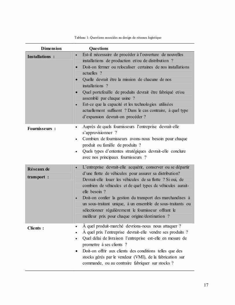
Plus concrètement, pour une entreprise ou groupe d’entreprises, le design de réseau
logistique vise à fournir des réponses à un ensemble de questions stratégiques; des exemples de
ces questions sont listées au Tableau 1.
17
Tableau 1: Questions associées au design de réseaux logistique
Dimension Questions
Installations : Est-il nécessaire de procéder à l’ouverture de nouvelles
installations de production et/ou de distribution ?
Doit-on fermer ou relocaliser certaines de nos installations
actuelles ?
Quelle devrait être la mission de chacune de nos
installations ?
Quel portefeuille de produits devrait être fabriqué et/ou
assemblé par chaque usine ?
Est-ce que la capacité et les technologies utilisées
actuellement suffisent ? Dans le cas contraire, à quel type
d’expansion devrait-on procéder ?
Fournisseurs : Auprès de quels fournisseurs l’entreprise devrait-elle
s’approvisionner ?
Combien de fournisseurs avons-nous besoin pour chaque
produit ou famille de produits ?
Quels types d’ententes stratégiques devrait-elle conclure
avec nos principaux fournisseurs ?
Réseaux de
transport :
L’entreprise devrait-elle acquérir, conserver ou se départir
d’une flotte de véhicules pour assurer sa distribution?
Devrait-elle louer les véhicules de sa flotte ? Si oui, de
combien de véhicules et de quel types de véhicules aurait-
elle besoin ?
Doit-on confier la gestion du transport des marchandises à
un sous-traitant unique, à un ensemble de sous-traitants ou
sélectionner régulièrement le fournisseur offrant le
meilleur prix pour chaque origine/destination ?
Clients : À quel produit-marché devrions-nous nous attaquer ?
À quel prix l’entreprise devrait-elle vendre ses produits ?
Quel délai de livraison l’entreprise est-elle en mesure de
promettre à ses clients ?
Doit-on offrir aux clients des conditions telles que des
stocks gérés par le vendeur (VMI), de la fabrication sur
commande, ou au contraire fabriquer sur stocks ?
18
La détermination de la configuration permettant de maximiser le profit de l’entreprise sur
un horizon de planification couvrant plusieurs années s’avère une tâche très complexe. Comme le
font remarquer, exemples à l’appui, Geoffrion and Powers (1995), l’intuition humaine s’avère
insuffisante pour optimiser le design d’un réseau logistique, c.-à-d. pour trouver celui qui permet
de maximiser le profit anticipé. La présente thèse s’inscrit dans le domaine de recherche associé
au design de réseaux logistiques, visant à déterminer, pour une entreprise donnée, le design
optimal. On parlera donc du problème d’optimisation du design d’un réseau logistique.
1.2 Terminologie et concepts clés
Bien qu’une grande partie de l’apport de notre domaine de recherche porte sur la
formulation de problématiques de design de réseau sous formes de modèles mathématiques et sur
la résolution de ces modèles d’optimisation, on aurait tort de croire que l’effort se résume à
concevoir des méthodes de résolution de programmes mathématiques mixtes en nombres entiers
(MIP). Bien que les récents travaux dans notre domaine de recherche s’appuient notamment sur
les mathématiques appliquées et plus particulièrement sur la recherche opérationnelle, les
innovations en informatique et en algorithmique, de même que l’expansion des connaissances en
logistiques et en stratégie d’affaires ont contribué à l’avancée des connaissances en design de
réseaux logistiques.
De plus, les termes « problème », « modèle », « solution » et même « optimalité » sont
utilisés pour désigner des concepts différents dans différentes communautés scientifiques. Cette
section vise à préciser la signification des termes utilisés dans le cadre de cette thèse et à
positionner les grandes catégories de contributions scientifiques au domaine de recherche.
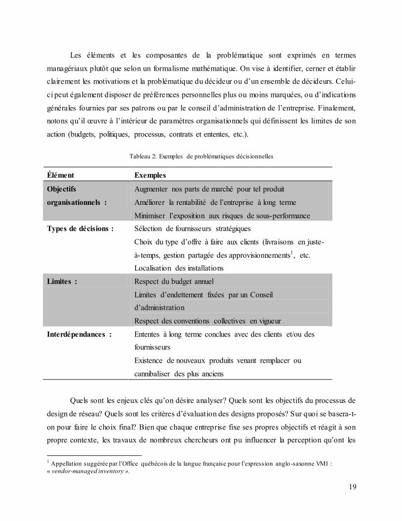
1.2.1 Problème de décision
Tout d’abord, l’expression « problème de décision » fait référence à l’ensemble d’une
problématique de prise de décision, telle que vue par un décideur (ou par un ensemble de
décideurs) dans un contexte organisationnel donné. Elle fait référence aux objectifs stratégiques,
ou aux buts, fixés par l’organisation, au type de décisions faisant l’objet de l’analyse, aux limites
associées au pouvoir des décideurs ou aux interdépendances associées à ces décisions. Le
Tableau 2 ci-dessous présente des exemples de ces éléments.
19
Les éléments et les composantes de la problématique sont exprimés en termes
managériaux plutôt que selon un formalisme mathématique. On vise à identifier, cerner et établir
clairement les motivations et la problématique du décideur ou d’un ensemble de décideurs. Celui-
ci peut également disposer de préférences personnelles plus ou moins marquées, ou d’indications
générales fournies par ses patrons ou par le conseil d’administration de l’entreprise. Finalement,
notons qu’il œuvre à l’intérieur de paramètres organisationnels qui définissent les limites de son
action (budgets, politiques, processus, contrats et ententes, etc.).
Tableau 2: Exemples de problématiques décisionnelles
Élément Exemples
Objectifs
organisationnels :
Augmenter nos parts de marché pour tel produit
Améliorer la rentabilité de l’entreprise à long terme
Minimiser l’exposition aux risques de sous-performance
Types de décisions : Sélection de fournisseurs stratégiques
Choix du type d’offre à faire aux clients (livraisons en juste-
à-temps, gestion partagée des approvisionnements1, etc.
Localisation des installations
Limites : Respect du budget annuel
Limites d’endettement fixées par un Conseil
d’administration
Respect des conventions collectives en vigueur
Interdépendances : Ententes à long terme conclues avec des clients et/ou des
fournisseurs
Existence de nouveaux produits venant remplacer ou
cannibaliser des plus anciens
Quels sont les enjeux clés qu’on désire analyser? Quels sont les objectifs du processus de
design de réseau? Quels sont les critères d’évaluation des designs proposés? Sur quoi se basera-t-
on pour faire le choix final? Bien que chaque entreprise fixe ses propres objectifs et réagit à son
propre contexte, les travaux de nombreux chercheurs ont pu influencer la perception qu’ont les
1 Appellation suggérée par l’Office québécois de la langue française pour l’expression anglo -saxonne VMI :
« vendor-managed inventory ».

20
autres chercheurs des tendances lourdes en design de réseau. Citons en exemple la définition
même de chaîne de valeur par Porter (1985), l’approche « Triple-A » de H. L. Lee (2004)
pronant l’agilité en matière de gestion de la chaîne logistique et celui de Christiensen, Raynor,
and Verlinden (2001), qui ne sont pas des articles portant à proprement parler sur les techniques
de design de réseau mais qui ont su identifier et influencer les tendances lourdes ayant des
impacts sur les décisions stratégiques en matière de logistique. Ci-après, nous utiliserons
l’expression « problème de décision » ou tout simplement « problématique » (en anglais, dans les
articles : «decision problem » ou tout simplement « problem ») pour faire référence à ce pilier du
design de réseau logistique.
1.2.2 Modélisation mathématique
La description des enjeux, des objectifs et des concepts importants associés à la chaîne de
valeur ne suffit pas pour obtenir des designs de réseaux performants. Geoffrion and Powers
(1995) affirment que l’utilisation et la résolution de modèles de design de réseaux logistiques
peut permettre de réduire les coûts logistiques d’une entreprise de 5% à 15%. La formulation
d’un modèle d’optimisation se fait en traduisant les objectifs et les critères d’évaluation en un
ensemble de fonctions objectifs, les limites quant à l’utilisation du réseau en contraintes et en
exprimant les choix à faire sous forme de variables de décision continues ou discrètes. Le nombre
d’articles scientifiques offrant des innovations de ce type est considérable. Bien que certains
auteurs utilisent le terme « problem » pour désigner certaines familles de modèles
mathématiques, nous préférons employer ici le terme modèle, qui permet de bien distinguer le
problème de décision et les modèle(s) formulés pour faciliter sa résolution.
Plus formellement, nous qualifierons de « modèle d’optimisation » ou plus simplement de
modèle, un ensemble de variables de décision et de paramètres numériques organisés de façon à
former un système de fonctions objectifs et de contraintes. Une « solution » est obtenue en
attribuant une valeur à chacune des variables de décision. Cette solution est dite réalisable si elle
satisfait toutes les contraintes du modèle, et non-réalisable si elle en viole au moins une. Une
solution réalisable est « optimale » s’il n’existe aucune autre solution permettant d’obtenir une
meilleure valeur pour la ou les fonctions objectifs.
21
Un modèle est toujours une abstraction plus ou moins précise ou exacte d’un problème de
décision donné; il cherche à capturer l’essence du problème sans s’encombrer de détails
accessoires. La formulation d’un modèle mathématique nécessite des choix de modélisation. Par
exemple, le nombre et la forme des objectifs ou fonctions objectifs influencera profondément la
nature du modèle. On dira qu’il est mono-objectif s’il comporte une seule fonction objectif et
qu’il est multi-objectif autrement. Ce modèle peut être linéaire ou non, convexe ou non, et
comporter ou non des variables de décision binaires et/ou entières. Ces choix de modélisation ont
un impact déterminant sur la nature des algorithmes utilisés pour résoudre les modèles. Une revue
de littérature centrée sur la modélisation des problématiques de design de réseaux logistiques est
proposée au chapitre 2.
1.2.3 Algorithme d’optimisation
Quoique notre finalité soit d’élaborer une ou plusieurs solutions de qualité pour aider le
décideur à résoudre un problème de décision, ceci se fait indirectement en utilisant des
« méthodes de résolution » des modèles formulés. À cet égard, les problèmes de design de réseau
logistique sont d’une grande complexité et ont nécessité certaines approches no vatrices de
solution de programmes mathématiques mixtes de grande taille.
Plus précisément, nous désignons par « algorithme d’optimisation » un ensemble ou suite
d’étapes ou d’opérations définies ayant pour but de produire une ou plusieurs solutions pour un
modèle d’optimisation donné. Idéalement on souhaite obtenir la solution optimale associée à un
modèle d’optimisation, ou une solution proche de cet optimum. Nous utilisons le terme
« méthode exacte » pour désigner tout algorithme d’optimisation garantissant de converger vers
la solution optimale en un temps fini.
1.2.4 Interrelations entre problématique, modèle et algorithme
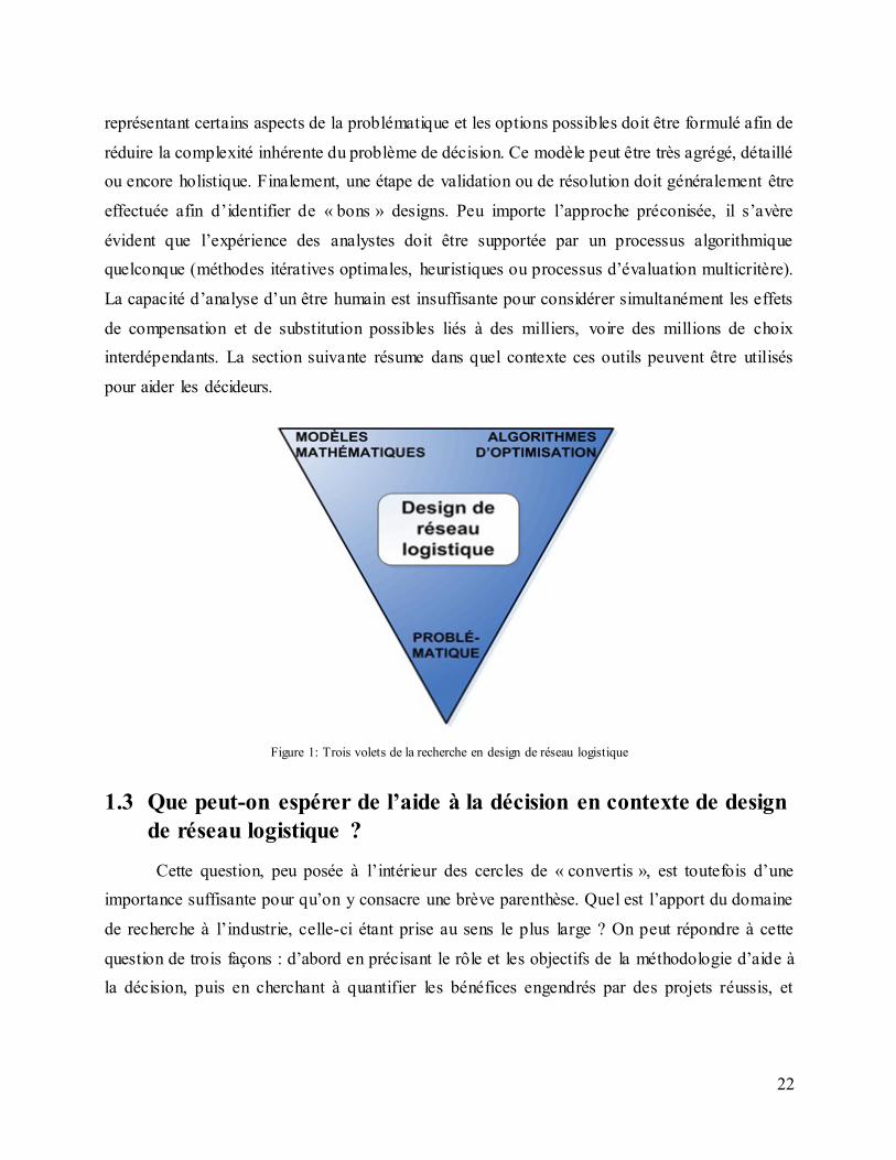
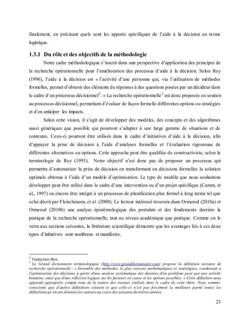
Au-delà des domaines mis à contribution, la recherche en matière de design de réseau logistique
repose sur trois volets méthodologiques principaux. La très forte majorité des articles publiés
dans notre domaine proposent des innovations dans au moins l’un des trois volets. Ces trois
piliers fondamentaux sont représentés à la figure 1.
Ces trois volets sont cruciaux afin d’outiller le décideur dans sa prise de décision. Tout
analyste doit bien comprendre la situation de l’entreprise, ses objectifs stratégiques et
opérationnels, son environnement interne et externe et la nature de ses opérations. Un modèle
22
représentant certains aspects de la problématique et les options possibles doit être formulé afin de
réduire la complexité inhérente du problème de décision. Ce modèle peut être très agrégé, détaillé
ou encore holistique. Finalement, une étape de validation ou de résolution doit généralement être
effectuée afin d’identifier de « bons » designs. Peu importe l’approche préconisée, il s’avère
évident que l’expérience des analystes doit être supportée par un processus algorithmique
quelconque (méthodes itératives optimales, heuristiques ou processus d’évaluation multicritère).
La capacité d’analyse d’un être humain est insuffisante pour considérer simultanément les effets
de compensation et de substitution possibles liés à des milliers, voire des millions de choix
interdépendants. La section suivante résume dans quel contexte ces outils peuvent être utilisés
pour aider les décideurs.
Figure 1: Trois volets de la recherche en design de réseau logistique
1.3 Que peut-on espérer de l’aide à la décision en contexte de design
de réseau logistique ?
Cette question, peu posée à l’intérieur des cercles de « convertis », est toutefois d’une
importance suffisante pour qu’on y consacre une brève parenthèse. Quel est l’apport du domaine
de recherche à l’industrie, celle-ci étant prise au sens le plus large ? On peut répondre à cette
question de trois façons : d’abord en précisant le rôle et les objectifs de la méthodologie d’aide à
la décision, puis en cherchant à quantifier les bénéfices engendrés par des projets réussis, et
23
finalement, en précisant quels sont les apports spécifiques de l’aide à la décision en terme
logistique.
1.3.1 Du rôle et des objectifs de la méthodologie
Notre cadre méthodologique s’inscrit dans une perspective d’application des principes de
la recherche opérationnelle pour l’amélioration des processus d’aide à la décision. Selon Roy
(1996), l’aide à la décision est « l’activité d’une personne qui, via l’utilisation de méthodes
formelles, permet d’obtenir des éléments de réponses à des questions posées par un décideur dans
le cadre d’un processus décisionnel2. » La recherche opérationnelle3 est donc proposée en soutien
au processus décisionnel, permettant d’évaluer de façon formelle différentes options ou stratégies
et d’en anticiper les impacts.
Selon cette vision, il s’agit de développer des modèles, des concepts et des algorithmes
aussi génériques que possible qui pourront s’adapter à une large gamme de situations et de
contextes. Ceux-ci pourront être utilisés dans le cadre d’initiatives d’aide à la décision, afin
d’appuyer la prise de décision à l’aide d’analyses formelles et l’évaluation rigoureuse de
différentes alternatives ou options. Cette approche peut être qualifiée de constructiviste, selon la
terminologie de Roy (1993). Notre objectif n’est donc pas de proposer un processus qui
permettra d’automatiser la prise de décision en transformant en décisions formelles la solution
optimale obtenue à l’aide d’un modèle d’optimisation. Le type de modèle que nous souhaitons
développer peut être utilisé dans le cadre d’une intervention ou d’un projet spécifique (Camm, et
al., 1997) ou encore être intégré à un processus de planification plus formel à long terme tel que
celui décrit par Fleischmann, et al. (2008). Le lecteur intéressé trouvera dans Ormerod (2010a) et
Ormerod (2010b) une analyse épistémologique des postulats et des fondements derrière la
pratique de la recherche opérationnelle, tant au niveau académique que pratique. Comme on le
verra aux sections suivantes, la littérature scientifique démontre que les avantages liés à ces deux
types d’initiatives sont nombreux et manifestes.
2 Traduction libre.
3 Le Grand dictionnaire terminologique (http://www.granddictionnaire.com) propose la définition suivante de
recherche opérationnelle : « Ensemble des méthodes, le plus souvent mathématiques et statistiques, conduisant à
l'optimisation des décisions à partir d'une analyse systématique des données d'un problème posé par une activité
humaine, ainsi que d'une réflexion logique sur les facteurs en cause et les options possibles. » Cette définition nous
apparaît appropriée compte tenu de la nature des travaux réalisés dans le cadre de cette thèse. Nous sommes
conscients que d’autres définitions existent et que celle-ci n’est pas forcément la meilleure parmi toutes les
définitions qu’en ont données les auteurs au cours des soixante dernières années.
24
1.3.2 Des bénéfices engendrés par l’aide à la décision en contexte de design de
réseau logistique
On peut aussi montrer la pertinence de la discipline en présentant des cas d’entreprises ou
d’organisations ayant réussi à améliorer leur profitabilité de façon considérable en appliquant les
recommandations issues d’un processus d’aide à la décision comprenant la résolution de modèles
mathématiques. Nous tablons ici sur des économies réelles et non sur des économies anticipées
telles le profit estimé à l’aide de la solution optimale d’un modèle mathématique.
Tout d’abord, Geoffrion and Powers (1995) indiquent qu’au cours de leur expérience
académique et commerciale comprenant des interventions pour le gouvernement des États-Unis
d’Amérique ainsi que pour plus de 50 entreprises, « il a été possible de réduire les coûts de
distribution de 5% à 15% tout en maintenant ou améliorant le niveau de service offert à la
clientèle4 ». La liste des entreprises et des bénéfices encourus n’est évidemment pas disponible.
La littérature scientifique regorge toutefois d’exemples plus spécifiques.
Arntzen, Brown, Harrisson, and Trafton (1995) décrivent un cas d’application fort
intéressant, où l’implantation d’un réseau logistique suggéré par la solution d’un modèle
mathématique linéaire mixte (MIP) a permis à l’entreprise DEC 5 de réaliser des économies
supérieures à 100 millions de dollars américains (USD), sur un chiffre d’affaires annuel de 14
milliards USD réalisé dans 81 pays.
Camm, et al. (1997) décrivent une initiative d’ampleur similaire réalisée chez la
multinationale Procter & Gamble (P&G) lors de la restructuration de sa chaîne logistique en
Amérique du Nord; l’implantation des conclusions tirées du modèle mathématique ont engendré
des charges de transition de plus de 1 milliard USD, affectant plus de 50 familles de produit, 60
usines et 10 centres de distribution. Au net, les chercheurs affirment que l’initiative a permis de
réaliser des économies récurrentes de plus de 200 millions USD.
Denton, Forrest, and Milne (2006) présentent un projet réalisée chez IBM affectant la
chaîne logistique des semi-conducteurs. Parmi les bénéfices listées dans l’étude, on identifie
notamment une augmentation des produits livrés à temps de 15% et une réduction des inventaires
de 25% à 30%. Les auteurs concluent que « plutôt que de déterminer un point optimal sur la
courbe de compromis service-inventaire, l’initiative a permis le déplacement complet de la
courbe » (op.cit.). D’autre part, Ulstein, Christiansen, Grønhaug, Magnussen, and Solomon
4 Traduction libre de « In most cases, we have been able to reduce distribution costs by five to 15 percent while
maintaining or improving customer service ». (Geoffrion et Powers, 1995). 5 DEC : Digital Equipment Corporation.
25
(2006), dans le cadre d’une étude réalisée pour la firme norvégienne Elkem, cite une
augmentation des revenus nets d’exploitation de 9 à 21 millions USD sur deux ans dans un
contexte économique défavorable (taux de change élevé et baisse du prix de vente des produits
sur le marché mondial).
Notons également que Bell, Anderson, and Kaiser (2003) ont conduit une étude
longitudinale (5 ans) sur 34 applications de recherche opérationnelle ayant obtenu le statut de
finalistes ou gagnants du concours du prix Edelman, volet secteur privé, entre 1989 et 1998. Au
terme de leur étude, Bell, et al. (2003) concluent que 20 de ces 34 applications ont permis à
l’entreprise impliquée de développer un avantage comparatif durable.
1.3.3 Des apports de l’aide à la décision en contexte de design de réseau
logistique
Au-delà des bénéfices engendrés par l’application directe d’une solution issue d’un
modèle mathématique, Geoffrion et Powers (1995) affirment d’entrée de jeu que « l’action de
bâtir un modèle complet a permis [à de nombreuses organisations] d’avoir une meilleure
compréhension de leur dimension logistique6 ». J. F. Shapiro, Singhal, and Wagner (1993) font
un constat similaire. Les mêmes auteurs indiquent que les étapes de préparation et de validations
des données produisent des bénéfices distincts de ceux obtenus suite à l’application d’une
solution issue d’un modèle mathématique.
D’autres études, telles Fleischmann, Ferber, and Henrich (2006) chez BMW et Kabakaral,
Günal, and Ritchie (2000) pour l’entreprise Volkswagen indiquent que les modèles
d’optimisation développés et résolus ont permis d’identifier des opportunités significatives en
termes de réduction des coûts, sans toutefois chiffrer les économies réellement obtenues par
l’entreprise. Dans le même ordre d’idées, Köksalan and Süral (1999) concluent, suite à une étude
menée pour Efes Beverage Group que « notre expérience dans ce projet et dans d’autres indique
que la solution optimale en elle-même a une valeur limitée. Les décideurs bénéficient de
l’opportunité de comparer différentes solutions7 […]. »
C’est donc dire qu’au-delà de l’implantation directe des solutions proposées par les
modèles, l’ensemble du processus menant à la formulation d’un modèle, à la fixation de ses
6 Traduction libre de: « […] the very act of building a comprehens ive model has helped most of these organizations
to understand their logistical dimension more profoundly. » 7 Traduction libre de: « Our experience in this and other projects shows that obtaining the optimal solution alone has
very limited benefits. The decision makers usually benefit from the opportunity to compare different solutions and
appreciate it more. »

26
paramètres et l’étude des solutions obtenues par celui-ci peut permettre d’identifier des pistes
d’amélioration substantielles pour l’entreprise.
1.4 Objectifs et structure de la thèse
Cette thèse contribue à l’avancée des connaissances relatives aux volets « modélisation » et
« résolution » du schéma présenté à la figure 1. Plus précisément, les objectifs suivants sont
identifiés :
1. Concevoir une méthode de solution permettant de traiter des problèmes d’optimisation
combinatoire de grande taille comportant plusieurs types de décisions et la tester sur une
classe de problèmes;
2. Proposer une approche générique combinant plusieurs innovations récentes en design de
réseaux logistique dans un modèle décisionnel intégré, et proposer un modèle
mathématique associé à cette approche;
3. Utiliser la méthode de résolution développée (objectif #1) afin de résoudre des problèmes
de design de réseau logistique en contexte déterministe multi-périodes;
4. Adapter la méthode de résolution développée à la résolution de problèmes de design de
réseau logistique en contexte stochastique multi-périodes.
La thèse comporte trois articles, en plus d’une revue de littérature; celle-ci est présentée
aux chapitres 2 et 3. Le premier article, présenté au chapitre 4, propose CAT (Collaborative
Agents Team), une méthodologie générique pour résoudre des problèmes d’optimisation
complexes de grande taille comportant plusieurs dimensions. Le cas d’application de cet article
traite également du design de réseau logistique en contexte déterministe.
Le deuxième article, présenté au chapitre 5, propose une approche de modélisation par
activité pour résoudre le problème de design de réseaux logistiques en contexte déterministe
multi-périodes. Un échantillon d’instances est résolu avec CAT et ces résultats sont comparés à
ceux obtenus à l’aide du solveur générique CPLEX. Cet article a été accepté pour publication
dans la revue International Journal of Production Economics.
Le troisième article, inséré au chapitre 6, propose une approche de programmation
stochastique pour le problème de design de réseaux logistiques en contexte d’incertitude. Il décrit
le modèle mathématique utilisé ainsi que les hypothèses quant à la nature des incertitudes.
27
Finalement, il propose des adaptations à la méthode CAT afin de lui permettre de résoudre des
modèles d’optimisation stochastiques de grande taille.
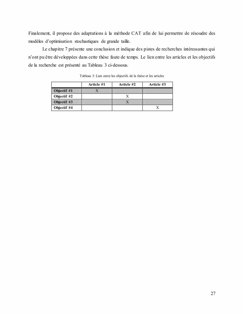
Le chapitre 7 présente une conclusion et indique des pistes de recherches intéressantes qui
n’ont pu être développées dans cette thèse faute de temps. Le lien entre les articles et les objectifs
de la recherche est présenté au Tableau 3 ci-dessous.
Tableau 3: Lien entre les objectifs de la thèse et les articles
Article #1 Article #2 Article #3
Objectif #1 X
Objectif #2 X
Objectif #3 X
Objectif #4 X
28
2 The design of supply chain networks
This chapter presents a review of the relevant literature on Supply Chain Network (SCN)
design problems and models. Different representations and formalizations of the decision
problem are presented and discussed. The chapter does not pretend to be exhaustive. An
overview of the literature is proposed, describing the key elements of modern SCN design
models, and discussing the implications, drawbacks or weaknesses associated to these models.
Section 2.1 introduces the concept of distributed decision making (DDM) that is especially
relevant to this thesis and to the design models discussed. Section 2.2 discusses the main
elements and key decisions associated to a SCN design model, and links to examples of these
elements already proposed in the literature. Section 2.3 describes some shortcomings of the
current SCN design literature.
2.1 Distributed decision making and SCN design
As mentioned in the introduction of this thesis, supply chains incorporate myriads of
actors, decision-makers and components that seldom come from monolithic organizations.
Distributed decision making (DDM) (Schneeweiss, 2003), is a theoretical framework that helps
to understand decision systems composed of a large number of interrelated decisions made by
several decision-makers More formally, DDM refers to the design and coordination of connected
decision problems. Supply chain design and management, in particular, can be seen as a set of
interconnected decision problems: production planning and scheduling, distribution planning,
transportation planning, sourcing and procurement, etc. In a business context, these decisions are
often made at different times and using different planning horizons (resulting in information
asymmetry) and by different decision makers with different goals and spheres of influence
(resulding in hierarchy among some decisions). In SCN design, this hierarchy is extremely
important, as strategic decisions define the very structure of the supply chain that will be used by
operational managers and logisticians on a day-to-day basis. Failing to take into account the
operational impacts of SCN design decisions may be hazardous, as saving on strategic capital
expenses may result in increased operational costs and reduced flexibility or customer service.
The conceptual framework associated with distributed decision making (DDM) sheds
light on an important reality of SCN design decision problems that influences optimization
29
models. Since the design decisions have such an outstanding impact on the operation of the
supply chain, it is necessary to include some of the operational dimensions in SCN design models
in order to be able to evaluate the quality of a potential SCN design.
According to this, decision variables of typical SCN design models can be divided into
two subsets:
Variables that represent the (strategic) design decisions regarding the supply chain
structure. These are the decisions that must be made and implemented.
Variables that approximate the usage of the resulting SCN design at the operational level.
These variables do not correspond to decisions that will actually be implemented (product
flows in a supply chain are rarely fixed on an annual basis, but instead result from
business processes such as replenishement, order processing, and produc tion and
distribution scheduling), but are necessary to assess the quality of a potential SCN design.
In terms of DDM systems, these variables and their associated constraints are an
anticipation of the actual SCN usage decision made by the operational managers. The
sub-model that corresponds to these decisions and constraints is often labeled as the
anticipated user model. The norm in SCN design models is to use annual flows and
throughputs.
This form of anticipation is necessary for a number of practical and theoretical reasons:
1. Modeling operational decisions of an entire supply chain into a realistic-sized SCN
design model would result in an intractable model;
2. Since operational decisions in a supply chain are numerous and diverse, and since
they can be reviewed multiple times before being implemented (such as when using
rolling horizon planning techniques), it is very difficult to build a set of simulation or
optimization models that would accurately predict the individual operational decisions
that would be made when using a potential SCN.
3. Usage decisions are made at a later time than SCN design decisions, when a lot more
information about costs, product orders from clients, inventories, and capacities will
be available. This phenomenon is called time-based information asymmetry in DDM
systems.
30
This last element is especially important. In essentially means that even if the supply
chain management models associated to SCN usage decisions were integrated into a huge SCN
design model and this model would be solvable using some state-of-the-art algorithms, the
resulting model would still be an approximation of the real SCN usage. In most deterministic
single-period SCN design models, this hierarchical information asymmetry is implicit and not
discussed by the authors. Even when these modeling decisions are implicit, the study of DDM
systems provides insights on the limitations of selected model. Moreover, DDM systems are very
useful to understand three categories of SCN design models:
1. Multi-season and multi-period models, where time-related information asymmetry is
present;
2. Models with multiple decision makers (in cooperative or noncooperative contexts) where
information and power asymmetry is especially important;
3. Models dealing with uncertainty (robust models, or multi-stage stochastic optimization
models).
A recent study of SCN design models using various forms of anticipated user models
shows that more detailed and accurate user models enhances SCN design model quality at the
cost of increased complexity (Klibi, Martel, & Guitouni, 2010b). Viewing SCN design models as
DDM systems is also in concordance with SCN design literature. As mentioned in Dogan and
Goetschalckx (1999), the goal of SCN design is to support strategic- level decision making in the
context of SCN management. This is in accordance with the modern notion of strategic
management, which consists of setting long-term business goals and actions that orient tactical
and operational decision making in a given organization (Porter (1985); Hafsi, Séguin, and
Toulouse (2000)).
2.2 Characteristics of SCN design models
The design of SCN is based on a set of inter-related decisions which cannot be partitioned
or separated into completely independent sub-problems. This section analyses different trends
and evolutions in SCN design models published in the scientific literature. These evolutions or
improvements are discussed for the decision categories present in typical SCN design models.
The order of presentation of the various SCN design model elements is borrowed from Martel
(2005), with additional elements inserted where appropriate.

31
The importance of supply chains in general, and of supply chain design, in particular, is
largely known and accepted (Goetschalckx, 2011; J. F. Shapiro, 2007). Societies, corporations
and individuals have always faced the location and resource allocation decisions that form the
basis of the field now labeled as supply chain network design. These decisions can be conscious,
well-defined, formalized and based on strategic and/or numerical analysis, or they can be largely
informal. The associated decision processes are also heavily dependent on culture, context, and
the availability of formal methods and models (Carle, 2008).
This section focuses on the evolution of SCN design models rather than on the evolution
of supply chain strategy or management strategy. In order to be classified as a SCN design
problem, three decision types must be present in the decision problem:
1. Location decisions, specifying which sites and facilities will be used among a set of
possibilities. These decisions may include facility reconfiguration or expansion decisions;
2. Mission assignment or allocation decisions, specifying which activities (parts
manufacturing, sub-assembly, final assembly, distribution, packaging, etc.) should be
performed at each facility;
3. Product, information and/or monetary flows resulting from the usage of supply chain.
According to this classification, categories 1 and 2 represent the true SCN design decisions while
decisions from category 3 represent the anticipated user model.
2.2.1 Organizational context
The organizational context refers to the structure of the business environment and the
domain convered by the SCN design problem. A decision problem is usually defined under a
specific context, consisting of a set of goals or values as well as environmental and organizational
conditions and structure. Specifically, the number of decision makers, the cooperative or non-
cooperative (antagonistic) nature of their relationship and whether the model is designed to cover
the operations of a single company or a supply chain consisting of multiple companies,
considerably affects how the problem will be modeled.
2.2.1.1 Wholly-owned supply chains
Most SCN design models proposed in the literature implicitly assume that the problem
must be solved by a single decision-maker which has the authority and responsibility of
designing a single company’s entire supply chain or its distribution network. In this context, the
32
decision-maker is assumed to be ubiquitous: he has complete control over the supply chain, has
perfect information about costs, capacities and objectives, and operates under the assumptions of
a pure top-down hierarchy between the strategic and operational levels, the absence of any
conflicting goals within the company, and the absence of explicit reaction from either the
operational level, the company stakeholders or its competitors. This assumptions prevail for
publications on capacitated facility location (Beasley, 1993; Jacobsen, 1983), distribution system
network design (Jayaraman & Ross, 2003; Ross & Jayaraman, 2008), and SCN design (Geoffrion
& Graves, 1974; Paquet, Martel, & Desaulniers, 2004).
2.2.1.2 Multi-division enterprises
In some contexts, large multinational firms are divided into two or more divisions or
subsidiaries which are responsible for either a subset of the company’s markets (countries, sales
territories or regions) or products. In most of these contexts, the divisions have some autonomy
on some SCN design decisions, while the firm as a whole exherts some form of coordination.
According to Holmberg (1995), this coordination is done through the allocation of shared
resources (such as capital budgets) or the fixation of prices (such as transfer prices for products
between divisions). There is a rich literature on the design of organizational structures and control
mechanisms in the context of multi-division enterprises through solving optimization models
(Burton and Obel (1980), Van de Panne (1991), Holmberg (1995), Tind (1995)) and supply chain
management (Kiekintveld, Miller, Jordan, and M.P. (2006), Albrecht (2010)). The literature on
SCN design models generally assume a divisional structure and use transfer prices. Some models
also optimize transfer prices (Goetschalckx & Vidal, 2001; M’Barek, Martel, & D’Amours,
2010). Yet, these models assume that all decisions are taken at the top level and exact execution
of the SCN usage decision by the divisions. In the context where divisions are profit centers and
the divisional managers are accountable for their division’s performance, each division may have
some incentives to optimize its own profit over the profit of the firm as a whole. This issue is
typically not addressed by SCN design model in the literature.
2.2.1.3 Multi-firm supply chains
Assessing the coordination of decisions across a supply chain characterized by multiple
ownership structures is very different than under the single- firm structure. Information exchange
is limited between the supply chain partners in order to protect each company’s interests and
33
competitive advantages. The goal of the supply chain is to design coordination mechanisms
through information exchange and/or the setting of contracts.
In certain contexts, one of the firms has enough influence to force adoption of a single
centralized planning model, even if multiple competing firms are part of the planning process.
Shirodkar and Kempf (2006) describe such an application, where a collaborative capacity
planning initiative between computer chip manufacturer Intel and six of its key suppliers resulted
in two integrated planning models: a tactical one-year capacity planning model as well as a 5-
year strategic planning model. It is, to the best of my knowledge, the only application of multi-
firm centralized SCN design planning. Another way to achieve collaboration is through the
establishment of supply contracts, on which there exists a lot of literature. The reader is refered to
Cachon (2003) for a detailed discussion on supply chain contracts. In general, however,
coordinated SCN design between several partners belonging to a given value chain has not been
addressed in the literature. There is, however, a rich body of literature on collaboration and
synchronization of operational- and tactical- level decisions. Different coordination mechanisms
could be explored, such as negotiation (Dudek & Stadtler, 2005), collaboration with cost sharing
(Frisk, Jornsten, Gothe-Lundgren, & Ronnqvist, 2010) or by using more detailed anticipations in
SCN design models. Reviews and detailed discussion of recent work in supply chain
collaboration mechanisms can be found in Stadtler (2009) and Albrecht (2010).
2.2.2 Evaluation of the supply chain performances
There is a rather abundant literature now on what are the qualities that characterize an
“excellent” supply chain. H. L. Lee (2004) coins this type of supply chain as “Triple-A”: agile,
adaptable and aligned. Martel (2005) focuses on achieving competitive advantage, defined as
being able to consistently maintain one or more order winning critera over its competitors,
whether it be low costs, delivery time, product quality or flexibility. Through the concept of a
“portfolio of supply chains”, Olavson, Lee, and DeNyse (2010) highlight the need for global
supply chains to possess different skills such as speed and cost efficiency. A qualitative analysis
of supply chain strategy in relation to overall business strategy can be found in H. L. Lee (2002).
When modeling supply chain networks, however, attributes such as “agility”, or
“adaptability” cannot easily be converted to metrics that can be incorporated into an optimization
model. While most authors acknowledge that several characteristics are desirable from a supply
34
chain point of view, two approaches are traditionally used to model the SCN decision maker’s
goal: mono- and multi-objective.
2.2.2.1 Mono-objective models
The rationale behind using a model with a single objective can be justified for its
desirable properties as well as its (relative) simplicity. It makes it possible to use a wide variety
of optimization algorithms to find optimal or quasi-optimal solutions, from commercial solvers to
decomposition techniques and metaheuristics. It reduces the need for a decision maker to
subjectively assign weight factors to multiple critera, to sort them in a lexicographical order or to
evaluate trade-offs between pareto-optimal solutions. Approximations and linearization
techniques are often used to achieve a mixed- integer linear (MIP) or linear (LP) model that can
be effectively solved to optimality (Martel, 2005).
Objective functions of mono-objective models are always money-based. Depending on
the nature of the SCN design decisions to make and the amount of authority the decision-maker
has over the supply chain, different objective functions can be used. In some business contexts,
product prices, marketing policies and are already fixed; this can even be the case for product
demands that can be fixed through the negociation of contracts. In this case, the objective
function consists of minimizing relevant logistics costs, such as supply and raw materials, facility
location and capacity expansion, transportation, production, and distribution costs. Arntzen et al.
(1995), Dogan et Goetschalckx (1999) and Paquet et al. (2004), among others, propose SCN
design models that belong to this category. Different relevant costs are computed and modeled,
depending on the business context that is modeled.
When product demand is not fixed a priori or the demand is assumed to vary according to
several factors such as product quality, order-to-delivery time, product price, or other market-
based considerations an economic value-added (EVA), net profit, or residual cash flow
maximization objective function can and should be used. Of course, it may not be possible to
estimate the impact of different lead-times, unit sales price modification or demand shaping
actions on demand or gross revenue functions. However, if this information exists, it should be
incorporated into the optimization model. Lead-time considerations are usually included in the
model in the form of constraints to be satisfied by the solution. By using different maximum
acceptable lead-times and running the model multiple times, one can plot an effic ient frontier, as
shown in case a) from Figure 2, borrowed from Martel (2005). Under a profit maximization
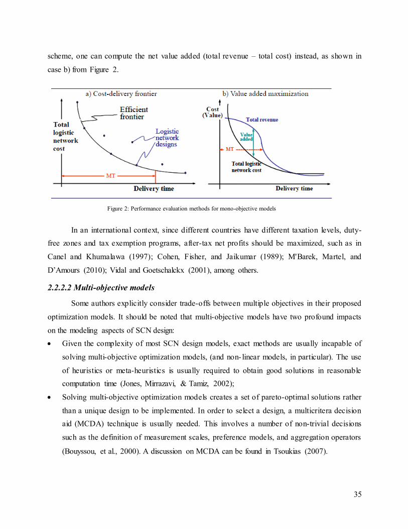
35
scheme, one can compute the net value added (total revenue – total cost) instead, as shown in
case b) from Figure 2.
In an international context, since different countries have different taxation levels, duty-
free zones and tax exemption programs, after-tax net profits should be maximized, such as in
Canel and Khumalawa (1997); Cohen, Fisher, and Jaikumar (1989); M'Barek, Martel, and
D’Amours (2010); Vidal and Goetschalckx (2001), among others.
2.2.2.2 Multi-objective models
Some authors explicitly consider trade-offs between multiple objectives in their proposed
optimization models. It should be noted that multi-objective models have two profound impacts
on the modeling aspects of SCN design:
Given the complexity of most SCN design models, exact methods are usually incapable of
solving multi-objective optimization models, (and non- linear models, in particular). The use
of heuristics or meta-heuristics is usually required to obtain good solutions in reasonable
computation time (Jones, Mirrazavi, & Tamiz, 2002);
Solving multi-objective optimization models creates a set of pareto-optimal solutions rather
than a unique design to be implemented. In order to select a design, a multicritera decision
aid (MCDA) technique is usually needed. This involves a number of non-trivial decisions
such as the definition of measurement scales, preference models, and aggregation operators
(Bouyssou, et al., 2000). A discussion on MCDA can be found in Tsoukias (2007).
Figure 2: Performance evaluation methods for mono-objective models
36
These two drawbacks did not discourage several authors from proposing multi-objective
SCN design models, even if several of these papers do not address the concerns mentioned above
(especially impact #2). A review of the relevant literature shows that all multi-objective models
include either the minimization of relevant costs or the maximization of net revenues as one of
the objectives. Other objectives vary from application to application:
Zhou, Min, and Gen (2003) as well as Olivares-Benitez, Gonzalez-Velarde, and Rios-
Mercado (2010) consider a customer service that is inversely proportional to the average
transit time between warehouses and clients.
Altiparmak, Gen, Lin, and T.Paksoy (2006) consider two additional objectives: a
customer service criteria and capacity utilization balance between the different facilities
of a network. Pishvaee, Farahani, and Dullaert (2010) use the same customer service
critera in their bi-objective model.
Wang, Huang, and Dismukes (2005) consider multiple objectives derived from SCOR
model level-1 metrics (SCOR, 2012): delivery reliability, flexibility and responsiveness,
costs, and assets utilization.
Liu and Papageorgiou (2012) consider minimization of total flow time for products as
well as the minimization of lost sales due to lack of capacity or other factors.
Ding, Benyoucef, and Xie (2009) consider financial and logistics-based objectives in a
simulation approach. However, the actual objectives are not discussed in detail in their
paper.
Fahimnia, Luong, and Marian (2009) use an additional objective that consists of
minimizing the violation of four types of constraints.
Cintron, Ravindran, and Ventura (2010) use five objectives: profit maximization, lead
time minimization, customer power, credit performance, and distributor reputation. The
three later objectives are seldom justified and rely on the rating of distributors and
consumers according to non-defined aggregation, preference or utility functions.
Azaron, Brown, Tarim, and Modarres (2008) as well as Venkatadri, Bose, and Azaron
(2012) incorporate profit variance and financial risk minimization as additional
objectives, in addition to cost minimization.
Of these applications, two families of critera are present in most applications: either (cost
minimization or profit maximization), and (customer service maximization or lead-time
37
minimization). Some authors argue that maximizing value creation implicitly optimizes all these
objectives (Martel & Klibi, 2012), and thus, maximizing profits and customer service in the same
model amounts to double counting. This debate is far from settled, and taking a stand in this
debate is outside the scope of this thesis.
2.2.3 Modeling of tactical and operational decisions
Although SCN design decisions form the core of SCN design models, section 2.1 outlined
the importance of approximating tactical and/or operational level decisions in a strategic model.
For the majority of SCN design models, this anticipated user model consists of period ic product
flows and a level of aggregation consisting of individual stock-keeping units (SKUs) (Liang &
Wilhelm, 2008) or product families, as in strategic models inspired by the hierarchical planning
paradigm (Hax & Candea, 1984; Schneeweiss, 2003). This anticipated user model corresponds to
approximations of a large number of isolated decisions that will be made later, often by different
decision makers. According to Klibi, et al. (2010b) a more detailed anticipated user model may
yield a model of increased fidelity and accuracy, often at the cost of an increase in model
complexity. Kremer, Schneeweiss, and Zimmermann (2006) reach similar conclusions while
analysing aggregate models used in the design of supply chain contracts.
Some authors proposed models with more detailed anticipated user models; however, the
SCN design models they solve are usually simpler than the most complex models with linear
annual product flows. Ko, Ko, and Kim (2006) investigate the distribution system network
design. A SCN design model selects the warehouses and 3rd-party logistic providers (3PLs) to be
activated as well as the allocation of customers to warehouses, while a detailed simulation model
is used to evaluate capacity utilization and service times. Once the simulation model is
completed, values of the SCN design model are updated until stable values are obtained. Klibi
and Martel (2012) propose several alternative user models for the stochastic location-
transportation model under disruptions, based respectively on scenario and period sampling and
decisions aggregation into a stochastic location-allocation model. They conclude that increasing
the quality of user models in SCN design may result in significant gains.
Aside from the work mentioned above, little has been done to incorporate more detailed
user-level anticipations in SCN designs models that cover the whole range of SCN design
decisions. There are significant research opportunities in the integration of detailed operational
models with strategic SCN design models.
38
2.2.4 Temporal representations
The very nature of strategic decisions requires that a planning horizon of several years
should be considered (Everett, Philpott, & Cook, 2000). Time periods is a concept used in the
literature to capture either the change in environmental conditions (demand, supply, etc.) over the
years or the change of network structure or mission allocation over different time horizons
(Martel, 2005). Several single-period mathematical models were proposed in the literature, such
as Geoffrion and Graves (1974), Pirkul and Jayaraman (1996), Goetschalckx and Vidal (2001)
and Paquet, et al. (2004). Single-period models are sometimes labeled as static models, while
multi-period models are labeled as dynamic models.
Different types of planning periods can be used. According to Martel (2005), multi-season
models capture the change in user decisions between different parts of a year (typically quarters
or months). This is especially important in seasonal industries such as in fashion or seasonal
clothing, where using annual time periods would fail to capture the inventory accumulation and
product price variation typical to these industries. Example of multi-season models are Arntzen,
et al. (1995) and Dogan and Goetschalckx (1999).
Multi-period models use a planning horizon encompassing several years. These models
have two main advantages. First, they can more accurately represent progressive changes in the
SCN structure over the years rather than a strict change / no change duality. Secondly, capital
investments such as the opening of a new factory are fundamentally long-term decisions, and
multi-period models allow for the evaluation of trade-offs between short-term revenues and
expenses versus long-term investments. An example of such SCN design model can be found in
Everett, et al. (2000), while a multi-period network redesign model is proposed by Melo, Nickel,
and Saldanha-da-Gama (2011, 2012).
For all their benefits, multi-period models have some serious drawbacks. Problem size
(number of decision variables and constraints) increases considerably with the number of time
periods used, which may even make the model inctractable. Furthermore, given the amount of
data necessary to build SCN design models, multi-period SCN design models require even more
data gathering and processing.
Finally, recent research has shown that multiple types of periods can be superposed to
model different time frames. Klibi and Martel (2009) use different time periods for SCN design
decisions and SCN usage, respectively. More generally, p lanning cycles can be used to model an
entire SCN reeingineering cycle, which can last from one to several years depend ing on the
39
company and industry. A planning cycle covers the horizon in which a SCN design decision is
made, implemented and used for some time before the network can be redesigned. S horter time
periods are used to model aggregate product flows and network usage decisions. These models
can help capture the evolving nature of SCN designs while keeping the model tractable and
solvable in reasonable amounts of time. As SCN planning models are often used on a rolling
horizon basis, usually, only decisions associated to the first reengineering cycle will actually be
implemented.
2.2.5 Uncertainty and risk modeling
The business environment is characterized by a certain degree of uncertainty. Sales
volume, market shares evolution, production factor costs or transportation costs may differ
substantially from forecasts. SCN design models are generated using large amounts of data, some
of which can be inaccurate. In particular, information regarding the future is uncertain. If actual
product demand or production costs differ substantially from forecasts, the selected SCN design
may be far than optimal.
Deterministic SCN design models assume that costs, revenues, prices, sales volumes and
capacities are known beforehand or can be forecasted with precision. Deterministic models can
be single-period (Geoffrion and Graves (1974), Pirkul and Jayaraman (1996)), multi-seasonal
(Arntzen, et al. (1995), Dogan and Goetschalckx (1999)), or multi-period (Paquet, Martel, and
Montreuil (2008), Melo, et al. (2011).
A stochastic SCN design model explicitly considers alternative plausible futures, often in
the form of a set of scenarios. This section considers modeling choices made in SCN design
decisions (see Birge and Louveaux (2011) for an introduction to stochastic programming).
Nickel, Saldanha-da-Gama, and Ziegler (2012) argue that “different sources of uncertainty exist
and can be included in [SCN design] models”. To the best of our knowledge, the seminal work of
Pomper (1976) is the most ancient work on stochastic SCN deign, and predates the emergence of
the term “supply chain”.
Different motivations may encourage a decision maker to rely on a stochastic model. One
may wish to design a supply chain that will be able to perform well under several market
conditions, a design goal put forward by D. H. Lee, Dong, and Bian (2010) as well as Nickel, et
al. (2012). Some decision makers may seek to protect the supply chain network against different
sources of disruptions caused by business (Qi, Shen, & Snyder, 2010) or environmental (Martel
40
& Klibi, 2011) distruptions such as natural catastrophes or terrorist attacks. Chopra, Reinhardt,
and Mohan (2007) distinguish between recurrent risks, which are associated with uncertain
delivery times, and disruption risks, which are related to supplier reliability, and advocate that
different mitigation strategies should be designed for each risk type. A detailed discussion of
elementary strategies to model uncertainty is found in Snyder (2006), while reviews of SCN
design issues are found in Mitra, Poojari, and Sen (2006) as well as Klibi, Martel, and Guitouni
(2010a).
Most models published in the literature follow one of two approaches. Some authors
propose so-called robust optimization models that are typically used to model stochastic facility
location or graph-inspired location models and include either minimax or regret-based objective
functions. Although an abundant literature exists on these approaches (Qi, et al., 2010; Snyder &
Daskin, 2006, 2007; Snyder, Daskin, & Teo, 2007), they are used to model very different
decision problems and they will not be discussed in detail in this literature review. A more
relevant approach which has been extensively used to model SCN design problems is stochastic
programming (Birge & Louveaux, 2011). The vast majority of models are two-stage stochastic
programs where SCN design decisions are made through (usually binary) first-stage variables,
while SCN usage is modeled through recourse (continuous) second-stage variables. Some
applications explicitly consider multi-stage models, such as Nickel, et al. (2012). Multi-stage
models are in general larger and more difficult to solve than two-stage stochastic programs.
Different approaches can be used to model the sources of uncertainty. Eppen, Martin, and
Schrage (1989) model uncertain parameters in the form of discrete probability distributions; as
such, the complete stochastic model can be solved directly through the formulation of the so-
called deterministic equivalent model (DEM). This approach is also used by other applications
such as Alonso-Ayuso, Escudero, Garin, Ortuno, and Perez (2003) However, several model
parameters are better represented using continuous probability functions, such as product
demands and production costs. Unfortunately, using continuous functions results in an infinite
number of scenarios. In that context, a deterministic-equivalent model cannot be formulated
directly. However, Monte-Carlo based sampling techniques such as the so-called Sample
Average Approximation (SAA) method (A. Shapiro, 2003) can be used in order to construct
samples of scenarios to approximate the stochastic problem for two-stage or multi-stage
programming. While theoretical analysis shows that for two-stage SAA models, one can obtain a
good-quality approximation of the true stochastic problem with a reasonable number of scenarios,
41
the size of the scenario sample required for the approximation of the true stochastic problem
within a certain error margin 0 with a probability 1 increases exponentially with the
number of stages in the model (Blomvall & Shapiro, 2006; A. Shapiro, 2006). Two-stage SAA
models are proposed in Santoso, Ahmed, Goetschalckx, and Shapiro (2005) as well as Vila,
Martel, and Beauregard (2007); this approach is also advocated in Martel and Klibi (2011).
2.2.6 Modeling activities, processes and products
Depending on the nature of products and supply chain activities, different modeling
strategies can be used. At the SCN design level, it is recommended to model aggregate high- level
activities (such as manufacturing, assembly, or packaging) rather than modeling each of the
multiple production sub-stages, which would result in unnecessary complexity. In the simplest
case, products are either not transformed by the supply chain, or a single raw product is
successively transformed into one unit of finished product. A supply chain where several finished
products can be manufactured from the same set of raw materials is labeled as either divergent or
one-to-many; this is frequently encountered in natural resources transformation such as in the
forest sector (Vila, Martel, & Beauregard, 2006). Discrete parts manufacturing (also labeled
many-to-one) supply chains can be modeled using acyclic graphs representing bills of materials
(Lakhal, Martel, Oral, & Montreuil, 1999). In the process industry such as pulp-and-paper
(M'Barek, et al., 2010; Philpott & Everett, 2001), multiple products can be manufactured using
different mixes of the same raw materials. The concept of recipe is thus used to model the
transformation of raw materials or intermediate products into finished products (M'Barek, et al.,
2010).
According to Paquet, et al. (2004), complex transformation processes can further be
modeled using technologies, which are defined by the set of products they can transform or store.
If more than one technology is available for a given activity/product pair, technology selections
can be incorporated in the SCN design model. According to Martel (2005), such technologies can
either be dedicated to a product family or be flexible enough to transform or store multiple
product families.
2.2.7 SCN representation
The notion of SCN representation refers to the approach used to model the structure of the
SCN, the company’s activities as well as the product flows over the network. Two alternatives
will be discussed: multi-echelon networks and general supply chain networks.
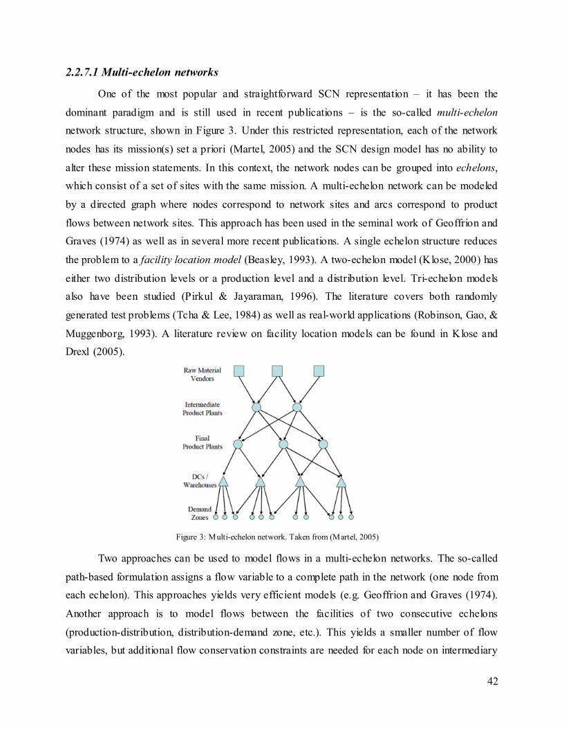
42
2.2.7.1 Multi-echelon networks
One of the most popular and straightforward SCN representation – it has been the
dominant paradigm and is still used in recent publications – is the so-called multi-echelon
network structure, shown in Figure 3. Under this restricted representation, each of the network
nodes has its mission(s) set a priori (Martel, 2005) and the SCN design model has no ability to
alter these mission statements. In this context, the network nodes can be grouped into echelons,
which consist of a set of sites with the same mission. A multi-echelon network can be modeled
by a directed graph where nodes correspond to network sites and arcs correspond to product
flows between network sites. This approach has been used in the seminal work of Geoffrion and
Graves (1974) as well as in several more recent publications. A single echelon structure reduces
the problem to a facility location model (Beasley, 1993). A two-echelon model (Klose, 2000) has
either two distribution levels or a production level and a distribution level. Tri-echelon models
also have been studied (Pirkul & Jayaraman, 1996). The literature covers both randomly
generated test problems (Tcha & Lee, 1984) as well as real-world applications (Robinson, Gao, &
Muggenborg, 1993). A literature review on facility location models can be found in Klose and
Drexl (2005).
Figure 4: Multi-echelon network structure
Two approaches can be used to model flows in a multi-echelon networks. The so-called
path-based formulation assigns a flow variable to a complete path in the network (one node from
each echelon). This approaches yields very efficient models (e.g. Geoffrion and Graves (1974).
Another approach is to model flows between the facilities of two consecutive echelons
(production-distribution, distribution-demand zone, etc.). This yields a smaller number of flow
variables, but additional flow conservation constraints are needed for each node on intermediary
Figure 3: Multi-echelon network. Taken from (Martel, 2005)
43
echelons. This approach can however model production environments where the nature of the
products changes at different echelons in the supply chains, while the path-based formulation
cannot.
Two trends are present in the literature. The first research trend is to develop more
efficient algorithms to either solve larger instances of the same model formulation or to solve the
same models in less computation time. This is especially present in single-echelon models, where
several methods have successively been published (Barahona & Chudak, 2005; Beasley, 1993;
Hansen, Brimberg, Urosevic, & Mladenovic, 2007; Kratica, Tosic, Filipovic, & Ljubic, 2001;
Kuehn & Hamburger, 1963; Michel & Van Hentenryck, 2004). The other trend is to extend an
existing model, usually by adding a new constraint type such as capacity levels on facilities
(Baker, 1982; Jacobsen, 1983) or single-sourcing constraints (Fisk, 1978).
Even if the multi-echelon approach is elegant, it has some severe limitations. In particular,
it forbids facilities to have more than one role, which can be far from optimal in some complex
multi-stage production processes (M’Barek, et al., 2010; Martel, 2005; Paquet, et al., 2004) such
as in the forest industry. Despite these serious drawbacks, multi-echelon models continue to be
used to address new SCN design problems, such as the introduction of a new product or product
family (Amini & Li, 2011), the progressive redesign of an existing SCN with budget constraints
(Melo, et al., 2011, 2012), and reverse logistics decisions (Alumur, Nickel, Saldanha-da-Gama, &
Verter, 2012). These models could be enhanced by being reformulated using an activity-based
approach.
2.2.7.2 General supply chain network
Another more recent approach is to let the model determine the missions of each facility.
In this family of models, some network nodes may have more than one mission, such as multi-
stage production plants or production-distribution centers. Although this approach produces more
complex optimization models, the assignation of site missions by the optimization model can
yield significant performance improvements. Examples of such models are found in (Amrani,
Martel, Zufferey, & Makeeva, 2011; Arntzen, et al., 1995; M'Barek, et al., 2010; Paquet, et al.,
2004).
Recent publications on network design are generally more concerned about incorporating
new modeling elements (decision types and constraints) than solving either larger instances or
providing better computation times on already published formulations. Examples of new
44
modeling constructs include technology selection (Paquet, et al., 2004), alternate facility
configurations (Amrani, et al., 2011), demand shaping actions (Vila, et al., 2007), greenhouse gas
emissions accounting and reduction (Chaabane, Ramudhin, & Paquet, 2012), integration of
reverse logistics (Chouinard, D’Amours, & Aït-Kadi, 2008), product life-cycle assessment (Hugo
& Pistikopoulos, 2005), transportation mode selection (Olivares-Benitez, et al., 2010) and fleet
size and mix (Miranda, Garrido, & Ceroni, 2009). Other publications model specific market
contexts such as oligopolistic markets (Masoumi, Yu, & Nagurney, 2012). Despite the simplicity
and popularity of multi-echelon models, it is hoped that general SCN design models will be
further used, since they are more general and flexible.
2.2.8 Modeling markets, demand, price and service
Most classical models from the literature assume that the demand for products is fixed a
priori, and is independent of the SCN configuration and the company’s strategic and tactical
efforts. While this assumption may be reasonable in some cases (in the context of planned
economies, in the context of a quota-based industry such as dairy products in the province of
Quebec, in product-markets with a price-demand elasticity of zero, or in industries which are
driven by long-term negociated contracts), it is clearly not realistic in the vast majority of
business contexts, especially at the international level or when a long planning horizon is
considered. Since the scientific literature seldom provides justification for this rather important
assumption, it is probably made to simplify the resulting model. Adequate modeling of demand
into SCN design models involves several challenges:
It may be difficult to accurately forecast the effect of demand shaping actions or
marketing policies on demand, especially when forecasting for multiple years;
Demand for a product is influenced by several factors, such as elements of a traditional
marketing policy (product characteristics, price, positioning and promotion), consumer
service, service levels and delivery times, the firm’s reputation (Kotler, Armstrong, &
Cunningham, 2011). It is also influenced by the competitors’ offers – which are difficult
to predict or anticipate – as well as the availability of substitude products.
It is highly desirable that any SCN design model that seeks to maximize economic value
added should incorporate a demand model. One approach is to use the modeling concept of
marketing policy proposed by Vila, et al. (2007). In this context, a marketing policy consists of a
global market offer for a given product-market by the company. It includes product prices,
45
service levels in term of maximum delivery time, required investments in promotion and other
marketing-based expenses, as well as other components of the market offer (such as vendor-
managed inventory), as well as sales expectations by product-market. Marketing policies are thus
selected by the SCN design model for each product-market. A marketing strategy based on next-
day delivery or vendor-managed inventory can have significant impacts on the supply chain
requirements (H. L. Lee, 2004, 2010). This concept can also be used to model potential contracts
in a business-to-business context; it could be further extended to include decisions such as
strategic positioning of inventories or decoupling points in complex supply chains.
Efforts have also been made to include competitors in SCN design models. Of course, as
competitors’ actions are difficult to predict with any accuracy, two approaches are used. One
approach is to assume those competitors’ actions are rational and risk-neutral, allowing the
application of microeconomic analysis and game theory such as Stackelberg and Cournot games.
This approach has been used in location analysis (Serra & ReVelle, 1994, 1995) which is closely
related to single-echelon models (Plastria, 2001). An extended model was later proposed that
includes product price setting decisions (Serra & ReVelle, 1999). Leader-follower (Stackelberg)
models have also been proposed (see Hakimi (1983) for the leader’s model and ReVelle (1986)
for the follower’s model). Game theory-based models were only recently extended to SCN design
models. Nagurney (2010) proposes a SCN design model under oligopolistic competition
formulated as a Cournot game; this model was later extended and applied to the pharmaceutical
sector (Masoumi, et al., 2012) as well as the fashion sector (Nagurney & Yu, 2012).
Another strategy is to anticipate possible actions or market offers from competitors and
assign a subjective probability to each of them (Vila, et al., 2007). These anticipative models
require some assumptions on competitors’ strategies but do not require the hypothesis of rational
or anticipational behavior. A two-stage stochastic model is then used, in which product demand
for the company’s products is influenced by the relative choices of demand shaping actions (first-
stage decision variable) as well as competitors’ actions which are observed in the second-stage.
This approach is promising, but it can require substantial – and potentially prohibitive – analysis
efforts, especially in the context of a multinational firm competing in several product-markets
each having lots of competitors8.
8 Procter and Gamble (P&G), PepsiCo and General Electic are good examples of such companies.
46
2.2.9 Modeling facilities and capacity options
Capacity expansion and facility location have always been central components to SCN
design models, from the earliest location models (Kuehn & Hamburger, 1963) to the more
sophisticated SCN design models (M'Barek, et al., 2010; Melo, et al., 2012). Most models make
a distinction between production capacity, which is decicated to a product (or product family),
and storage and distribution capacity, which is shared among all products (Geoffrion & Graves,
1974; Melo, et al., 2012), while Arntzen, et al. (1995) is a notable exception that considers
dedicated capacity for production and distribution.
The most simplistic approach to model facilities and capacities is to assume that the
layout (size, technologies and production capacity) of each facility (existing or potential) is given.
This approach is common in single-echelon (Beasley, 1993; Sankaran, 2007; Van Roy, 1986) and
multi-echelon models (Jayaraman & Ross, 2003; Melo, et al., 2011, 2012; Olivares-Benitez, et
al., 2010; Pirkul & Jayaraman, 1996). Furthermore, this approach fails to capture economies of
scale associated to larger production facilities or technologies (or results in a nonlinear model). In
practice, production and distribution facilities are usually composed of a set of diffe rent
production technologies in various numbers. In this context, fixing the layout of facilities a priori
may result in significantly sub-optimal SCN designs.
Paquet, et al. (2004) propose the concept of capacity options that can be installed into a
production or distribution site. Under this approach, capacity is not directly assigned to facilities.
A facility is associated to a certain number of square feet available to install different production
technologies or production/distribution systems. This allows the model to select between
different production or distribution technologies. Furthermore, for a given technology, different
capacity options can be used in order to model economies of scale. Martel (2005) observes that
facility layout can be designed to have fixed parts (that cannot be changed by the model) as well
as variable parts. Amrani, et al. (2011) propose the concept of alternative platforms. Each
platform represents an alternative configuration consisting of a set of technologies and capacities
(either shared or dedicated). It can be used to model changes to existing facilities or to model
potential facilities. In the context of multi-period models, upgrade platforms can be used which
consists of expansion or reconfiguration options. However, if there are a large number of
alternate facility configurations or the number of production technologies that can be used is very
large, the number of alternate platforms will result in the optimization model being too difficult
to solve.
47
2.2.10 Modeling product flows and inventories
In order to evaluate the quality of a SCN, it is desirable to approximate annual o r seasonal
production and distribution decisions through the use of aggregate product flows. Even if recent
research (Klibi, et al., 2010b) shows the limitations and drawback associated with such
aggregations, the inclusion of detailed raw materials purchasing, production scheduling,
distribution and routing decisions would make the design model untractable. Furthermore, the use
of annual product (or raw material) flows considerably simplifies the accounting of variable costs
and capacity utilization. Although some publications use detailed models to estimate product
flows, facility capacity, inventories and/or variable distribution costs (Klibi & Martel, 2012;
Klibi, et al., 2010b; Ko, et al., 2006), the vast majority of models use aggregate period flow
formulations (Altiparmak, et al., 2006; J. F. Cordeau, Pasin, & Solomon, 2006; Dogan &
Goetschalckx, 1999; Easwaran & Üster, 2010; Geoffrion & Graves, 1974; Goetschalckx & Vidal,
2001; Jayaraman & Ross, 2003; Melo, et al., 2011; Paquet, et al., 2004).
The modeling of inventories poses many challenges to SCN design models. A typical
supply chain will keep inventories for different functions. Inventories can be built up in
anticipation of demand increases in later period; this is important in seasonal industries where
production capacities are insufficient to meet demand at peak levels and where inventories are
accumulated accordingly. Cycle inventories are generated by the lotsizing of replenishement and
customer orders. Safety stocks protect against uncertainty in replenishement lead times.
According to Martel (2005), cyclic and safety stock levels depend on the management policies
used by the company, the ordering behavior of customers as well as replenishment lead times.
Furthermore, when sound inventory management principles are used, there is a risk pooling effect
resulting in a strictly decreasing marginal inventory-throughtput ratio (Martel (2002).
Furthermore, relationships between product inventory and throughput may be difficult to estimate
for new facilities or for new technologies in existing facilities.
As such, several models implicitly assume that inventory-throughput functions are linear
(Arntzen, et al., 1995; J.-F. Cordeau, Laporte, & Pasin, 2008; J. F. Cordeau, et al., 2006; Dogan
& Goetschalckx, 1999; Geoffrion & Graves, 1974; Goetschalckx & Vidal, 2001; Pirkul &
Jayaraman, 1996; Santoso, et al., 2005; Thanh, 2008). The model provided in Martel (2005) takes
risk pooling effects into account but assumes that inventories are independent of lead times.
Finally, some models explicitly incorporate risk pooling and lead times, usually at the expense of
ignoring other SCN design decisions. Several authors consider only single-period, single-product
48
models (Park, Lee, & Sung, 2010; Romeijin, Shu, & Teo, 2007; Shu, Li, Shen, Wu, & Zhong,
2012; Sourirajan, Ozsen, & Uzsoy, 2007). Shu, Teo, and Shen (2005), Shen and Qi (2007) and
Qi, et al. (2010) consider a single retailer, and their model does not contain any location or
facility configuration decisions. To the best of my knowledge, no integrated general logistics
network design model takes into account lead times and risk pooling effects. Approximation of
non- linear inventory throughput functions by piecewise linearization can be considered as an
interesting compromise between model accuracy and solvability.
2.2.11 Cost modeling
Modeling of cost and revenues in SCN design models is important in many contexts. It is
also an element that is handled differently in different models, but these differences are seldom
discussed in research papers. Two key elements will be analyzed in this section, namely cost and
revenue allocation and fixed costs modeling.
To national and multinational supply chains, cost allocation between the different
facilities of the network is of prime importance. Typically, in SCN design models, variable costs
are assigned to flow variables. However, companies operating in more than one country – in
more than one state in the Unites States of America or in one than more province in Canada –
face different taxation levels for different parts of their supply chain. Often, the company is
divided into two or more national divisions that pay taxes in different countries. Additional
accounting is necessary to compute profits or net (after-tax) revenue for each national division, as
well as tariffs and duties when a product or component crosses a border. The allocation of
transportation costs between facilities located in different countries, as well as the setting of
transfer prices between national division can also be considered strategic decision variables
(Goetschalckx & Vidal, 2001). Several optimization models incorporating these elements were
recently proposed, such as Perron, Hansen, Le Digabel, and Mladenovic (2010). Detailed
discussions of implications of global supply chains in SCN design models can be found in
Goetschalckx and Vidal (2001); Martel (2005), while a review of the relevant literature can be
found in Meixell and Gargeya (2005).
In several SCN design and location-allocation models, the full cost of buying or
implementing a facility is charged in the decision model. As such, in single-period models, the
costs of building a facility are compared to variable costs for a one-year planning horizon. This
form of cost modeling can yield solutions that underestimate the optimal number of facilities to
49
open or operate. It also neglects the fact that, unlike variable costs such as transportation costs,
facility acquisition is in fact an investment that increases the company’s assets. In practice,
returns on investments of more than one year are common for strategic- level investments. Multi-
period models are better suited to evaluate trade-offs between facility acquisition costs and
annual costs and revenues.
An alternative approach is to split the facility cost into two parts. The implementation cost
consists of all costs that are inherent to setuping the facility costs and do not include capital
expenditure costs. It includes personnel hiring costs, support activities and the costs of relocating
equipment, etc. The exploitation cost consists as a rent paid for using the platform. If the facility
is actually rented, this corresponds to the rent payments made to the facility owners. In the case
of an owned facility, it corresponds to the amount the company would obtain if it rented the
facility to a 3rd-party. This covers capital expenditure costs, depreciation as well as tax returns,
and permits the evaluation of cost trade-offs on an annual basis.
2.2.12 Emerging trends
Aside from modeling costs, capacities, inventories and processes, there are a number of
emerging SCN modeling trends. Among them, the design of sustainable supply chain networks
has also recently received much attention. Pan, Ballot, and Fontane (2010) explore approaches to
reduce greenhouse gas emissions, and Chaabane, et al. (2012) develop a design model
integrating tradeoffs between environmental and economic objectives. Chouinard, et al. (2008)
and Easwaran and Üster (2010) consider the design of closed- loop supply chains, and a review of
the literature on reverse logistics network design is found in Ilgin and Gupta (2010).
2.3 Outstanding issues and shortcomings of the current literature
Since the publication of the first warehouse location models (Balinski, 1961; Kuehn &
Hamburger, 1963), significant progress has been made in the formulation of more realistic
location-allocation and SCN design models. However, some aspects have been covered
superficially in the literature, and several research avenues must be explored more thoroughly.
Several new models were proposed in recent publications. However, the following two remarks
on recent contributions show that research is more fragmented than ever:
Most new models improve upon previous work published by the same contributors but do not
integrate recent advances proposed by other authors. One example is the model of Melo, et al.
50
(2012), which builds upon a previously published model (Melo, Nickel, & Saldanha-da-
Gama, 2006) but completely ignores new modeling constructs such as activity graphs
(Lakhal, et al., 1999), technology selection options (Paquet, et al., 2004) or international
aspects (Goetschalckx & Vidal, 2001).
The absence of a common methodology, besides solving optimization models, and of a
common vocabulary. Two types of confusion are observed in the literature:
o Using the same words to describe different concepts or techniques. One obvious
example is the very scope of what labeled as supply chain design in the literature. In
some publications (Qi, et al., 2010), supply chain design problem are associated to
setting safety stocks and replenishement levels while in others it is associated to
technology selection, facility location and mission assignement (M'Barek, et al.,
2010).
o Using different words to refer to the same concepts. An example of this confusion is
in time horizon representation. The same formulation is labeled multi-period in
Arntzen, et al. (1995), while it is called multi-seasonal in Martel (2005).
Terminology such as chain-based or activity-based formulation is useful only if it is used
by all authors. This lack of unification is even more apparent when literature on SCN design
models is compared to other flourishing research sectors such as vehicle routing, for which
standard formulations, common terminology and even test instances sets exist. Literature reviews
help, but self-discipline from authors is also necessary.
Fragmentation has other undesired consequences. Several interesting modeling concepts
have been proposed in the recent recent literature (inventory modeling, marketing policies, cost
modeling, and capacity options); however, no publication has unified all these concepts into a
single, integrated model that could be used to address different SCN design problems from varied
industrial sectors. This model would likely be very difficult to solve, so specialized solution
methods would be needed.
Most strategic SCN models use very crude anticipated user model in the form of annual
product flows. Simulation models and operational decision models should be used to better assess
the impact of strategic decisions on the resulting SCN and to provide accurate feedback on
capacity usage, lead times, inventory levels and variable costs. That being said, implementing
such a detailed operational user model would require substantial amounts of data as well as
51
simulation or optimization models to represent the various activities and the interactions between
activities in the supply chain.
Finally, when modeling strategic decision problems, uncertainty should be taken into
account. The assumption that long-term future can be forecasted with accuracy is rather
unrealistic. Markets evolve quickly; costs of production factors (such as energy prices) fluctuate
substantially, even over short-term horizons. Stochastic programming seems an appropriate
methodology to represent a set of plausible futures into an optimization model. The resulting
integrated two- or multi-stage multi-period stochastic models are of course very difficult to solve,
as the most recent and thorough deterministic optimization models are already large and
complex.
52
3 Optimization algorithms used to solve SCN design models
This chapter presents a review of the relevant literature on optimization algorithms, with a
focus on methods that can be used to solve SCN design models. A review of solution methods
that have been used to solve SCN design models is first provided. This section is followed by a
discussion on solution methods that are promising for the solution of large-scale SCN design
models but that have not been proposed yet in the literature.
Note that for the purpose of this chapter, we are only interested in optimization algorithms
designed to solve mixed-integer linear mathematical programming (MIP) models (and by
extension, linear programming (LP) problems as well as binary or integer (IP) models), as well as
mixed- integer nonlinear (MINLP) models9. As IP models can be reformulated as binary integer
programming models (Winston & Venkataramanan, 2003), without loss of generality, we refer to
MIP models in the following.
3.1 Exact approaches
Optimization methods are labeled as “exact approaches” if they can provably find the optimal
solution of an optimization model in a finite (possibly very large) amount of time. Explicit
enumeration of all solutions to IP models is totally impossible, even for models of 30-50 integer
variables (Wolsey, 1998). Most exact approaches use model decomposition, implicit enumeration
of the solutions tree or cutting plane generation techniques to solve the models efficiently.
3.1.1 Branch-and-bound
The branch-and-bound method is based on implicit enumeration of the solutions tree. Upper and
lower bounds on the objective function value of the optimal solutions are computed. Assume we
want to find the optimal solution to the maximization model S , with optimal solution *z . In the
case of a maximization problem, the upper bound z is provided by solving a (usually linear)
relaxation of the problem, while the lower bound z is provided by a feasible solution. The
branch-and-bound algorithm begins by solving the linear relaxation of the model, thus providing
an upper bound z . Assuming some of the integer variables are non- integer in the LP relaxation10,
9 According to Winston and Venkataramanan (2003), “a nonlinear integer programming [model] is an optimizat ion
model in which either the objective function or the left-hand side of some of the constraints are nonlinear functions
and some or all of the variable must be integers [or binaries]”. 10
If all the integer and binary variables have integer values in the LP relaxation, then the solution to the LP
relaxation is optimal for the MIP.
53
the branch-and-bound algorithm divides the model into two non- intersecating sub-models by
branching on a fractional variable. Assuming that the variable jx has a fractional value in the LP
relaxation, we define two submodels: 1 : j jS S x x x and 2 : j jS S x x x . It is
trivial to prove that 1 2S S and
1 2S S S . The sub-models 1S and
2S are then solved
recursively. When a node is found to be unable to provide a feasible solution, it is pruned, thus
reducing the size of the solutions tree. F1 presents a a branch-and-bound flowchart provided in
Wolsey (1998). A more advanced discussion of branch-and-bound, along with thorough
examples can be found in Wolsey (1998) and Winston and Venkataramanan (2003).
In the branch-and-bound algorithm, two important decisions must be performed, among others:
1. The choice of node to examine;
2. The choice of the branching rule to apply.
These decisions are very important. In practice, branch-and-bound algorithms have been used to
solve single-echelon (Gao & Robinson, 1994) and multi-echelon (Tcha & Lee, 1984)
uncapacitated facility location models, multi-product two-stage facility location models (Hindi &
Basta, 1994; Hindi, Basta, & Pienkosz, 1998) as well as four-stage models (Georgiadis, Tsiakis,
Longinidis, & Sofioglou, 2011). Custom branch-and-bound algorithms also have been proposed
to solve multi-stage SCN design models (Ahmed, King, & Parija, 2003).
3.1.2 Cutting Plane Algorithms and Branch-and-cut
Instead of relying on branch-and-bound algorithms, another approach is to approximate the
convex hull of the polytope defined by an optimization model. In practice, this approximation is
done through the successive generation of valid inequalities. An inquality, or cutting plane
0x is said to be a valid inequality for X S if 0x is true for all x X . In practice,
interesting valid inequalities cuts feasible regions of the LP relaxation of X while removing
none of the MIP-feasible solutions. Although pure cutting planes algorithms have been proved to
converge to the optimal solution in finite time (Gomory’s algorithm (Gomory, 1963) converges
when the objective function is integer valued, this work has been further extended by Chvàtal
(1973) and by (Nemhauser & Wolsey, 1990) for MIP models in general). However, pure cutting
plane algorithms have not been very successful in general. However, valid inequalities can be
very effective when combined with branch-and-bound techniques. In several publications, valid
inequalities are often referred to as cuts.
54
According to Wolsey (1998), a branch-and-cut algorithm “is a branch-and-bound algorithm in
which cutting planes are generated throughout the branch-and-bound tree.” Rather than to explore
as many nodes as possible as quickly as possible, a branch-and-cut algorithm seeks to provide the
tightest possible bounds ( z and z ) at each node of the tree, using preprocessing, heuristics, or
cutting plane generation techniques. Of course, in practice, a trade-off between cut generation
and node exploration must be reached. A sample branch-and-cut algorithm detailed in Wolsey
(1998) is presented in F2 below.
There are a large number of cuts that can be applied to general MIP models. Furthermore, the
effective implementation of cutting plane techniques requires substantial efforts 11 (Gu,
Nemhauser, & Salvesbergh, 2000). Some of the most used MIP cuts are:
Gomory mixed-integer cuts (Balas, Ceria, Cornujéols, & Natraj, 1996; Gomory, 1960);
Flow cover inequalities (Gu, Nemhauser, & Salvesbergh, 1999);
Mixed-integer rounding cuts
Furthermore, several cuts have been proposed for specific MIP models or families of models that
exhibit a special structure (knapsack inequalities, for instance) or to solve specific problems
arising in a small number of models, such as symmetry cuts implemented in the Gurobi solver
(Bixby, Rothberg, & Gu, 2010). Typical SCN design models have complex structure which
makes the application of polyhedral approaches very challenging; to the best of my k nowledge,
pure cutting plane algorithms were not proposed to solve such models.
3.1.2.1 Commercial branch-and-cut based solvers
Special attention should be given to commercial MIP solvers such as CPLEX® and Gurobi®. As
general-purpose solvers, they are able to solve virtually any LP or MIP model, given enough
time, processing power and memory. A decision maker or analyst with limited knowledge of
optimization algorithms could thus use a generic MIP solver to find the optimal solution to his
model. Although they are based on the branch-and-cut paradigm, commercial solvers are use a
mix of several known techniques (cutting plane generation, MIP heuristics such as feasibility
pump (Fischetti, Glover, & Lodi, 2005) or local branching (Fischetti & Lodi, 2003)) as well as a
number of unpublished custom algorithms. This makes impossible further classification of those
11
In particular, some valid inequalities require either (1) a lifting procedure to be fact-defining or (2) the solving of a
separation sub-problem to define the actual values of and 0 .
55
algorithms beyond the fact that they are hybrid branch-and-cut algorithms. Performance of
commercial solvers can and should be used as benchmarks for specific purpose algorithms and
approaches. In general, for a specific purpose optimization algorithm to be of any interest, it must
at the very least be as efficient as the most efficient general-purpose solver available.
Solver performance may be slow for SCN design models, especially with default settings. A
number of acceleration techniques were used by some others, such as replacing default
parameters by specific values derived from empiric experimentation (Vila, et al., 2007), or adding
custom valid inequalities to strengthen the LP relaxation (Melkote & Daskin, 2001; Paquet, et al.,
2008). Some realistic-sized instances of supply chain network design models were solved to
optimality in reasonable computation times by (Vila, et al., 2006, 2007).
3.1.3 Lagrangian relaxation
The so-called Lagrangian relaxation is a decomposition technique that relies on relaxing a
number of “complicating” constraints, which usually makes the model especially difficult to
solve. In practice, these constraints are often integrated in a modified objective function by
penalizing their violation through the use of a real-valued vector u, which is often referred to as
the lagrangian multiplicators. Once the complicating constraints are dualized, the resulting
relaxed model is usually easy to solve (a LP model, a model solvable through dynamic
programming or by inspection, or an IP for which strong cutting planes are known such as the
knapsack model). The actual values of lagrangian multipliers to use are determined by solving a
lagrangian dual sub-model (Wolsey, 1998).
Lagrangean relaxation has been used by several authors to solve several facility location problem
variants. Marin (2007) solves two-stage uncapacitated facility location models by relaxing the
flow conservation constraints (that link the two stages of the problem), while Klose (2000) solved
the capacitated version by relaxing the capacity constraints. This approach has also been used as
a heuristic procedure by terminating the algorithm prior to convergence to an optimal solution,
thus creating so-called lagrangian heuristics (Avella, Boccia, Sforza, & Vasil'ev, 2009; Park, et
al., 2010)
Lagrangian relaxation can also be used in stochastic programming. Typically, the so-called non-
anticipativity constraints are relaxed, resulting in sub-problems that are decomposable on a
scenario-by-scenario basis (Mitra, et al., 2006).
56
3.1.4 Primal decomposition techniques
Another popular approach to solve complex SCN design models is the so-called Benders’ (or
primal) decomposition (Benders, 1962). The Benders’ decomposition strategy partitions the
model into two sub-models: one relaxed master model containing a set of “complicating”
variables (variables that makes the complete model especially difficult to solve) and a sub-model.
In the case of SCN design, the (relaxed) master model typically includes the strategic design
binary variables associated to facility location, technology selection or transportation / sourcing
option selection. The master model is first solved, and the values of the binary variables are then
transferred to the (hopefully) linear sub-model. If the sub-model is feasible, an optimality cut is
generated and added to the master model; if it is not feasible, a feasibility cut is added to the
master model instead.
In their seminal work, Geoffrion and Graves (1974) demonstrated the effectiveness of primal
decomposition techniques to solve SCN design models 12 . The largest model they solved had
more than 11,000 variables, including 757 binaries, which was extremely large considering the
limited memory available in computers in the early 1970s. Similar implementations of Benders’
decomposition have been used in numerous deterministic SCN design models, such as Dogan and
Goetschalckx (1999), Paquet, et al. (2004) and J. F. Cordeau, et al. (2006). The same algorithm
(which is called the L-shaped method (Van Slyke & Wets, 1969) in stochastic programming
literature) has also been used by Gutierrez, Kouvelis, and Kurawala (1996) and MirHassani,
Lucas, Mitra, Messina, and Poojari (2000), to solve stochastic SCN design models. Santoso, et
al. (2005) note that the addition of valid inequalities to the model may significantly decrease
computation times required to obtain an optimal solution to their sample average approximation
(SAA) models.
Some authors have used both primal and dual decomposition approaches in what is called cross
decomposition (Van Roy, 1983). This technique has been quite effective at solving capacitated
facility location models of size up to 100 facilities and 200 customers (Van Roy, 1986). For
instance, Kratica, et al. (2001) achieve similar computation times on instances of comparable size
with a far more powerful computer. Unfortunately, for SCN design models with more complex
structures, it is quite difficult to find “easy” dual and primal sub-models in order to implement
12
According to Google Scholar (http://scholar.google.ca), this paper has been cited more than 900 times.
57
cross decomposition. It might explain why the method has not been used often despite the
convincing results achieved by Van Roy (1986) and (C. Y. Lee, 1991).
3.1.5 Other exact approaches
Among the other approaches used to solve facility location and SCN design models, Martel and
Venkatadri (1999) and Martel (2005) use a technique called successive mixed-integer linear
programming to solve SCN design models under economies of scale, which are captured by
nonlinear functions in the constraint matrix. This approach involves the approximation of non-
linear functions by linear functions. Branch-and-fix is a variant of the branch-and-cut approach
that has been proposed by Alonso-Ayuso, Escudero, Garin, et al. (2003) for stochastic SCN
design models. Other decomposition algorithms have been proposed in the literature: Liang and
Wilhelm (2008) use Dantzig-Wolfe decomposition in a branch-and-price framework to design
production-assembly-distribution systems, while Shi, Meyer, Bozbay, and Miller (2004) use a
nested partitions approach.
Approximation algorithms have been proposed for uncapacitated (Cornuejols, Fisher, &
Nemhauser, 1977) and capacitated (Levi, Shmoys, & Swamy, 2004) location models. Another
approximation algorithm has been proposed by Ahmed and Sahinidis (2003) for the multi-stage
stochastic capacity expansion model, which is a restriction of the stochastic SCN design model.
Two research opportunities arise: either this algorithm could potentially be adapted to solve some
SCN design models, or it could be included to solve capacity expansion sub-models within a
more general optimization algorithm for the stochastic SCN design model.
3.2 Heuristics
In contrast to exact approaches, heuristics are solution methods that are aimed to find reasonably
“good” solutions in a reasonable time. According to Talbi (2009), in general, heuristics do not
have an approximation guarantee on the obtained solutions. However, they do have some
significant advantages, as shown by Silver (2004): ease of implementation, speed, simplicity,
robustness to changes in model parameters, and ease of use within other (exact or heuristic)
methods. Indeed, several classes of heuristics do not require the objective function or constraint
matrix to have specific properties such as linearity or convexity. We will review three types of
heuristic approaches that are especially relevant in the solution of SCN design models.
58
3.2.1 Classical heuristics
Several heuristics are inspired from intuitive problem solving strategies; they are by far the
simplest solution methods that can be applied to model optimization. The simplest heuristic of all
is the so-called random heuristic, which for every decision variable, randomly selects a value
from all the possible values that can be taken by that variable. Albeit its obvious drawbacks, this
method is often used to find an initial solution in metaheuristic approaches such as genetic
algorithms (Kratica, et al., 2001).
Other popular classical approaches are the so-called greedy heuristics (Silver, 2004). Greedy
heuristics are constructive methods that iteratively build a solution by making a series of myopic
(locally optimal) choices. Starting from an empty solutions, at each step of the algorithm, the
algorithm selects a choice that will maximize the increase of the objective function, without
trying to anticipate its impact on future choices or reconsidering decisions made at earlier stages
(Papadimitriou & Steiglitz, 1982). Greedy heuristics have been extensively used for solving
uncapacitated (Kuehn & Hamburger, 1963) as well as capacitated (Jacobsen, 1983) facility
location models. The most common greedy heuristics used for facility location and SCN design
are ADD (which start with an empty solution and selects facilities) and DROP (which start with
all facilities being selected and them iteratively removes facilities from the solution). These
simple heuristics can be extended to create other methods: SWAP (Kuehn & Hamburger, 1963),
ALA (Cooper, 1964) and VSM (Cornuejols, et al., 1977; Jacobsen, 1983) are greedy heuristics
applied to facility location problems. In particular, swap-based heuristics form the backbone of
several tabu search algorithms designed for facility location models (Al-Sultan & Al-Fawzan,
1999; Michel & Van Hentenryck, 2004; Ohlemuller, 1997).
Albeit these heuristics yield solutions of poor quality compared to either metaheuristics or exact
methods, they are fast to implement and can be used to quickly obtain a feasible solution.
Moreover, the basic idea behind greedy heuristics can be applied to several contexts. For
instance, a greedy heuristic can be used to obtain a feasible solution to very constrained models
by seeking to minimize an infeasibility measure instead of seeking to optimize the objective
function.
59
3.2.2 Metaheuristics
The term “metaheuristics” refers to a set of optimization algorithms that were developed for the
most part in the 1980s and early 1990s. According to (Talbi, 2009), the term was proposed by
(Glover, 1986) and refers to “upper level general methodologies (templates) that can be used as
guiding strategies in designing underlying heuristics to solve optimization problems”. According
to this definition, a metaheuristics should be coupled with one (or possibly more) heuristics,
which it guides in order to prevent from being trapped in local optima. However, some authors do
not make such a distinction between the actual heuristic and the upper-level methodology, and
use the term “metaheuristics” to refer to the whole algorithm (Dréo, Pétrowski, Siarry, &
Taillard, 2006). Metaheuristics are especially well suited to discrete and combinatorial
optimization problems, and are among the most efficient methods for solving the facility location
problem (Michel & Van Hentenryck, 2004), the vehicle routing problem (J. F. Cordeau &
Laporte, 2005), and the location routing problem (Boccia, Crainic, Sforza, & Sterle, 2010),
among others. Finally, metaheuristics can be readily adapted and extended to handle
multiobjective or multimodal optimization (Dréo, et al., 2006).
Metaheuristics also suffer some drawbacks. In general, they provide no estimation of solution
quality compared to the optimum (lower or upper bounds) and do not compute an optimality gap.
This issue is especially relevant on decision problems for which exact methods are inefficient. As
such, metaheuristics are generally applicable where exact approaches are unable to provide an
optimal solution in reasonable time for real-sized instances.
A large number of metaheuristics have been proposed in the literature. Even if they come from
different physical or biological metaphors, metaheuristics are increasingly similar in terms of
implementation mechanisms (Taillard, Gambardella, Gendreau, & Potvin, 2001). The following
two sections review the most common single-solution based and population-based
metaheuristics, respectively.
3.2.2.1 Single-solution based metaheuristics
Also called trajectory methods or local search-based methods in the literature, single-solution
based metaheuristics (SSBM) iteratively improves a single solution. The basic idea is to start
from an initial solution, then move from that solution to the next, until a stopping criterion has
been met. Algorithm 1 adapted from (Talbi, 2009), provides a generic template for single-
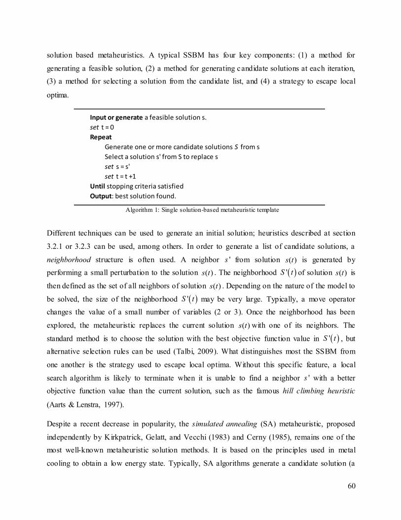
60
solution based metaheuristics. A typical SSBM has four key components: (1) a method for
generating a feasible solution, (2) a method for generating candidate solutions at each iteration,
(3) a method for selecting a solution from the candidate list, and (4) a strategy to escape local
optima.
Different techniques can be used to generate an initial solution; heuristics described at section
3.2.1 or 3.2.3 can be used, among others. In order to generate a list of candidate solutions, a
neighborhood structure is often used. A neighbor 's from solution ( )s t is generated by
performing a small perturbation to the solution ( )s t . The neighborhood 'S t of solution ( )s t is
then defined as the set of all neighbors of solution ( )s t . Depending on the nature of the model to
be solved, the size of the neighborhood 'S t may be very large. Typically, a move operator
changes the value of a small number of variables (2 or 3). Once the neighborhood has been
explored, the metaheuristic replaces the current solution ( )s t with one of its neighbors. The
standard method is to choose the solution with the best objective function value in 'S t , but
alternative selection rules can be used (Talbi, 2009). What distinguishes most the SSBM from
one another is the strategy used to escape local optima. Without this specific feature, a local
search algorithm is likely to terminate when it is unable to find a neighbor 's with a better
objective function value than the current solution, such as the famous hill climbing heuristic
(Aarts & Lenstra, 1997).
Despite a recent decrease in popularity, the simulated annealing (SA) metaheuristic, proposed
independently by Kirkpatrick, Gelatt, and Vecchi (1983) and Cerny (1985), remains one of the
most well-known metaheuristic solution methods. It is based on the principles used in metal
cooling to obtain a low energy state. Typically, SA algorithms generate a candidate solution (a
Input or generate a feasible solution s.
set t = 0
Repeat
Generate one or more candidate solutions S from s
Select a solution s' from S to replace s
set s = s'
set t = t +1
Until stopping criteria satisfied
Output: best solution found.
Algorithm 1: Single solution-based metaheuristic template
61
neighbor) randomly. If the candidate improves the objective function, it is accepted as the new
solution. If it degrades the objective function, it is nevertheless accepted with a certain
probability that depends on the actual degradation between the current and candidate solutions
and with a certain parameter, which is called temperature. At the beginning of the search, the
temperature (and thus the probability to accept degrading solutions) is high but decreases
monotonically during the search. Simulated annealing approaches have been successfully applied
to SCN design problems. (Ross, 2000) solve what is essentially a facility location model, while
Jayaraman and Ross (2003) and Ross and Jayaraman (2008) solve a distribution system design
model covering distribution and cross-docking centers. A recent survey on SA metaheuristics is
provided in Nikolaev and Jacobson (2010), while a more detailed discussion on SA can be found
in (Aarts & Korst, 1989).
Tabu search (TS) is a deterministic metaheuristic proposed by (Glover, 1986). Tabu search
behaves like the hill climbing heuristic, but it accepts the (best) nonimproving solutions to escape
local optima when all the candidate solutions are nonimproving. To avoid cycling between two
solutions, TS algorithms stores the inverse of the moves that were recently performed in what is
called a tabu list (Glover, 1989). The algorithm then forbids moves that are in the tabu list, in
order to prevent from returning to a recently visited solution. Various improvements over the
basic TS procedures proposed in Glover (1986) algorithms have been proposed in the literature,
having different types of memories to achieve better intensification and diversification (Talbi,
2009). However, the various TS algorithms applied to facility location and SCN design models
have a rather simple structure. Ohlemuller (1997), Al-Sultan and Al-Fawzan (1999), and Michel
and Van Hentenryck (2004) proposed TS algorithms for the uncapacitated facility location
model, while Sörensen (2002) considered the capacitated version (both deterministic and
stochastic). Tabu Search has also recently been applied to more complex multi-echelon SCN
design models (Melo, et al., 2012).
Iterated local search (ILS) is a memoryless metaheuristic proposed by Martin, Otto, and Felten
(1992) and formalized in Lourenco, Martin, and Stützle (2002) that starts with a feasible solution,
then applies local search on it such as the aforementioned hill climbing heuristic. When it reaches
a local optimum, a perturbation is applied to the solution before the local search heuristic is
applied again. The perturbation operator must be substantial in order to escape the local
optimum, (a.k.a. induce more change in the solution than the move operator). ILS has been
62
applied to a multi-echelon SCN design model with single assignment constraints by J.-F.
Cordeau, et al. (2008).
Variable Neighborhood Search (VNS) is a metaheuristic proposed by Mladenovic and Hansen
(1997) that consists of a systematic change in neighborhood combined with local search (Hansen,
Mladenovic, & Moreno Pérez, 2010). When the local search algorithm hits a local optimum, the
VNS algorithm switches to a new neighborhood definition and begins local search anew. A VNS
metaheuristic thus requires the use of at least two neighborhood structures, although most
implementations use more than two. A VNS metaheuristic has been applied successfully to the
multi-commodity SCN design with alternative facility configurations (Amrani, et al., 2011) as
well as the global supply chain design problem with transfer pricing (Perron, et al., 2010).
Single-solution based metaheuristics have shown their potential to solve several facility location
and SCN design models. They are especially suited to handle binary variables resulting from
facility location and configuration models, as these sets of variables can easily be organized into
neighborhoods. Various other metaheuristics have been proposed in the literature, but they are
not reviewed here as they have not yet been applied to SCN design problems.
3.2.2.2 Population-based metaheuristics
Rather than improving one solution at a time, population-based metaheuristics (PBM) seek to
improve a population of solutions. The algorithm starts by initializing a population of solutions;
these solutions are typically generated either randomly, by sampling of the decision space to
force diversity, or using some heuristics. At each iteration, new candidate solutions are generated
based on the features of solutions belonging to the current population. A new population is
generated using solutions from the current population of solutions as well as candidate solutions.
The population is thus evolved dynamically until one of the stopping criteria is met. A high- level
template for population-based metaheuristics adapted from Talbi (2009) is provided with
Algorithm 2.
Evolutionary algorithms (EA) are a family of population-based metaheuristics based on the
concepts of biological evolution developed by Charles Darwin. These metaheuristics have
evolved into distinct families of algorithms: genetic algorithms (GA) (Holland, 1975), evolution
strategies (ES) (Rechenberg, 1973), evolutionary programming (EP) (Fogel, Owens, & Walsh,
1966), genetic programming (GP) (Koza, 1992), estimation of distribution algorithms (EDA)
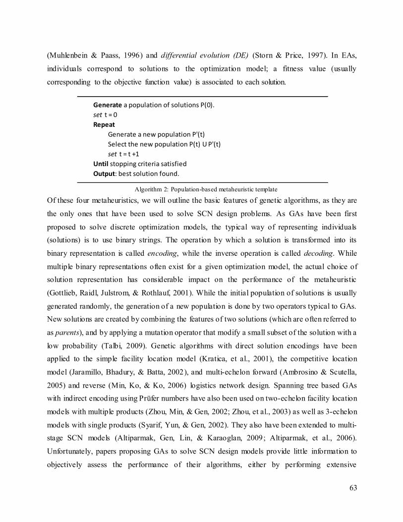
63
(Muhlenbein & Paass, 1996) and differential evolution (DE) (Storn & Price, 1997). In EAs,
individuals correspond to solutions to the optimization model; a fitness value (usually
corresponding to the objective function value) is associated to each solution.
Of these four metaheuristics, we will outline the basic features of genetic algorithms, as they are
the only ones that have been used to solve SCN design problems. As GAs have been first
proposed to solve discrete optimization models, the typical way of representing individuals
(solutions) is to use binary strings. The operation by which a solution is transformed into its
binary representation is called encoding, while the inverse operation is called decoding. While
multiple binary representations often exist for a given optimization model, the actual choice of
solution representation has considerable impact on the performance of the metaheuristic
(Gottlieb, Raidl, Julstrom, & Rothlauf, 2001). While the initial population of solutions is usually
generated randomly, the generation of a new population is done by two operators typical to GAs.
New solutions are created by combining the features of two solutions (which are often referred to
as parents), and by applying a mutation operator that modify a small subset of the solution with a
low probability (Talbi, 2009). Genetic algorithms with direct solution encodings have been
applied to the simple facility location model (Kratica, et al., 2001), the competitive location
model (Jaramillo, Bhadury, & Batta, 2002), and multi-echelon forward (Ambrosino & Scutella,
2005) and reverse (Min, Ko, & Ko, 2006) logistics network design. Spanning tree based GAs
with indirect encoding using Prüfer numbers have also been used on two-echelon facility location
models with multiple products (Zhou, Min, & Gen, 2002; Zhou, et al., 2003) as well as 3-echelon
models with single products (Syarif, Yun, & Gen, 2002). They also have been extended to multi-
stage SCN models (Altiparmak, Gen, Lin, & Karaoglan, 2009; Altiparmak, et al., 2006).
Unfortunately, papers proposing GAs to solve SCN design models provide little information to
objectively assess the performance of their algorithms, either by performing extensive
Generate a population of solutions P(0).
set t = 0
Repeat
Generate a new population P'(t)
Select the new population P(t) U P'(t)
set t = t +1
Until stopping criteria satisfied
Output: best solution found.
Algorithm 2: Population-based metaheuristic template
64
computational tests compared with another approach or by using the instances provided in
another paper. In particular, some researchers have shown that Prüfer number-based encodings
are inferior to other encodings such as permutations or edge lists (Gottlieb, et al., 2001).
Several other population based metaheuristics have been proposed in the literature: scatter search
(Glover, 1977; Resende, Ribeiro, Glover, & Marti, 2010), path-relinking (Glover, 1996; Resende,
et al., 2010), adaptive memory algorithms (Rochat & Taillard, 1995), as well as various
approaches inspired from nature that are collectively known as swarm intelligence. Of these
methods the most popular is arguably the ant colony optimization algorithm (Dorigo & Stützle,
2010). These methods have not yeed been applied to SCN design problems.
Parallel versions of popular metaheuristics such as GAs and Tabu Search have been proposed and
studied in the literature. With the increasing availability of multi-core processors, parallel
execution of algorithms seems a more natural and promising approach. Several software libraries
have been developed to ease the design and implementation of parallel meta heuristics, such as
ParadisEO (Cahon, Melab, & Talbi, 2004).
3.2.3 Heuristics based on mathematical programming
In contrast to the “classical” heuristics that are inspired from intuition and logic, some authors
developed heuristics based on exploiting the MIP formulation of the model13. The rationale
behind these heuristics is that a high-quality feasible solution helps keeping the branch-and-
bound tree small by pruning more nodes. These heuristics aim at (1) quickly providing an initial
feasible solution to the model and (2) finding high-quality feasible solutions without needing to
explore a large portion of the search tree. These strategies have been recently integrated into
commercial MIP solvers, to great results.
A large number of MIP heuristics have been proposed in the literature; see Ball (2011), for an
interesting yet incomplete review on the subject14. Three strategies are of particular interest: (1)
quickly reach a leaf of the branch-and-bound tree to obtain a feasible solution, (2) exploring the
region around an optimal solution to the LP relaxation of the model, (3) solving a mathematical
sub-model to generate a new (hopefully improved) feasible solution to the model and (4)
accelerate MIP convergence by progressively fixing binary or integer variables within the model.
13
We will restrict our discussion to heuristics that can be applied to mixed-integer linear programming models. 14
Several key papers are missing from this review such as the feasibility pump, local branching and RINS.
65
Several heuristics exploit the idea of fixing (or bounding) values of fractional variables in the LP
solution in an iterative matter (this approach is commonly refered to as diving). It effectively
simulates progressing from the root node to a leaf in the branch-and-bound tree, albeit a lot faster
(Bixby, Fenelon, Gu, Rothberg, & Wunderling, 2000). One of the most popular and powerful
application of this idea is the so-called strong branching rule (Achterberg, Koch, & Martin,
2005). Another example implemented in CPLEX is the guided dive heuristic (Danna, Rothberg,
& Le Pape, 2005). Diving heuristics are especially useful when facing models with a large
number of continuous variables in comparison to the number of binary variables.
Rounding the values of fractional variables in the optimal solution of a LP relaxation is a popular
and straightforward idea. However, directly rounding the values of all fractional variables in a
SCN design model may result in either unfeasible solutions (when fractions are rounded to 0) or
increased costs (when fractions are rounded to 1). Several heuristics are in fact elaborate
approaches for rounding LP-optimal solutions: pivot-and-shift (Balas, Schmieta, & Wallace,
2004), feasibility pump (Bertacco, Fischetti, & Lodi, 2007; Fischetti, et al., 2005), as well as
pivot, cut and dive (Eckstein & Nediak, 2007).
Some improvement heuristics use a feasible solution as a starting point, then finds additional
feasible solutions by solving sub-models. One of the most popular method is the so-called local
branching heuristic (Fischetti & Lodi, 2003), which defines a neighborhood around a feasible
solution at a given node of the branch-and-bound tree by limiting the number of variables that
can change values from the existing feasible solution. Additional variants and extensions such as
variable-depth branching (Cornillier, Pecora, & Charles, 2012) have been proposed since. This
Relaxation induced neighborhood search (RINS) defines a restricted MIP tha t consists of
searching a generic neighborhood constructed using the information contained in the LP
relaxation of the model (Danna, et al., 2005). Similar heuristics were proposed by Wilbaut and
Hanafi (2009).
Progressive variable fixing has been a popular strategy that has been applied to SCN design
problems. The idea is to fix some binary or integer variables using different critera, resulting in a
reduced model that is hopefully easier to solve. Variables are progressively fixed until the solver
returns an integral solution. Methods for generic MIP formulations often employ probing
techniques to select which variables should be fixed (Johnson, Salvesbergh, & Nemhauser, 2000;
66
Salvesbergh, 1994) When solving a specific class of optimization models, one can usually design
variable fixing rules that are both effective and sensible for that model, thus reducing the need
for probing. This approach has been used by Thanh, Péton, and Bostel (2010) as well as (Melo, et
al., 2011) for a multi-period SCN design model. However, Watson and Woodruff (2011) have
shown that an aggressive variable fixing scheme may result in severely reduced computation
times to solve large-scale MIPs.
3.3 Hybrid algorithms
Hybrid optimization algorithms integrate features from two or more optimization algorithms.
While hybrid algorithms are more complex and require more effort to implement, the strengths of
one method can compensate for the weaknesses of another. Two families of hybrids will be
reviewed: hybrid metaheuristics and hybrids between exact methods and metaheuristics. As the
number of applications of these methods to SCN design is relatively low, this section will cover
existing applications to SCN design as well as some hybrids that are promising for these models.
3.3.1 Hybrid metaheuristics
The concept of hybridizing two or more metaheuristics is well known and is the subject of many
works in the scientific literature; taxonomies have been proposed (Talbi, 2002, 2009), and entire
books have been published on that specific subject (Blum, Aguilera, Roli, & Sampels, 2008).
However, hybrid metaheuristics have not yet been proposed to solve complex SCN design
models. A few research opportunities can be outlined. In general, population-based
metaheuristics are good at searching different regions of the solutions space, while single-
solution based metaheuristics are good at intensification. SSBMs can be used to improve the
candidate solutions generated by population-based metaheuristics. An example of hybridization
between genetic algorithms and local search is memetic algorithms (Moscato & Cotta, 2010).
Furthermore, it is rather straightforward to construct neighborhoods to represent location
decisions in SCN design models. The hybridization of a VNS-based metaheuristic with TS or ILS
could yield good results.
3.3.2 Hybrids between exact methods and metaheuristics
The hybridization of metaheuristics and exact methods is a rapidly expanding field. The term
matheuristics has recently been coined to refer to combinations of metaheuristics and
mathematical programming methods (Raidl & Puchinger, 2008). According to Raidl (2006),
67
hybrids can be characterized by the (1) the types of algorithms used, (2) the level of
hybridization, (3) the execution scheme (parallel, sequential or interleaved) and (4) the control
strategy. A very interesting hybrid optimization algorithm for the simple facility location model
is the primal-dual VNS of Hansen, et al. (2007). In this algorithm, VNS is applied on both the
primal and dual side to generate tight bounds, then an exact method (sliding simplex followed by
a branch-and-bound) is used to obtain a final solution. Instances of size up to 15,000 facilities and
15,000 clients are solved to optimality with this method.
The vast majority of potential hybrid solution methods have not yet been tested on SCN design
problems. Due to the large number of optimization algorithms (heuristics, exact methods and
metaheuristics) available, the number of possible combinations of hybrid algorithms is relatively
huge. Explicit enumeration and testing of each possible combination does not seem to be an
effective strategy. However, the following hybridizations seem especially promising:
Embedding mathematical programming to explore neighborhoods to optimality in a TS or
VNS metaheuristic. Product flow variables (continuous variables) would be handled by a
linear programming algorithm while binary variables (supplier selection, facility location
and configuration) would be fixed by the metaheuristic.
Using hybrids between classical decomposition techniques and metaheuristics, by solving
the master problems and/or sub-problems arising in a given decomposition approach
using metaheuristics. Guidelines are provided in and Boschetti, Maniezzo, and Roffilli
(2010).
Using metaheuristics especially designed to handle MIP formulations such as the
parametric tabu search variants of Glover (2006) as well as Pedersen, Crainic, and
Madsen (2009). Similar hybrids using VNS have been recently proposed for feasibility
(Hanafi, Lazic, & Mladenovic, 2010a) and optimality (Hanafi, Lazic, Mladenovic,
Wilbaut, & Crévits, 2010b; Lazic, Hanafi, Mladenovic, & Urosevic, 2010).
Using classical and MIP-based heuristics to generate initial solutions of a population
based metaheuristic, while applying local search to newly generated solutions.
3.3.3 Agent-based algorithms
Multi-agent systems (MAS) and agent-based optimization algorithms have also been used
recently to model and analyse complex decision problems. Typically, MAS formalize complex
68
decision problems as networks of simpler decision problems, each of these problems being
tackled by a separate agent (Schneeweiss, 2003). Depending on the degree of sophistication of
the approach, the agent may use basic decision rules to make decisions, or formulate an
optimization model which is then solved with an appropriate (exact or heuristic) optimization
algorithm. Agents are in principle autonomous, have their own representation of the problem, and
make their own decisions on when to work and what to work on.
MAS can also be used to model decision problems where several decision makers are each
responsible for one part of the problem. This situation is rather common in supply chain
coordination problems (Gaudreault, Frayret, & Pesant, 2009). Even then, MAS can be useful for
modeling and solving centralized planning problems such as SCN design 15 . The approach
consists in dividing the problem into simpler sub-problems, and to assign each sub-problem to
one or more agents. The solutions produced by each of these agents are then combined into
solutions to the complete problem.
A relevant example of this approach is Asynchronous Teams (A-Teams) (Talukdar, Murthy, &
Akkiraju, 2003), a cooperative MAS used on various decision problems which evolves a
population of solutions in a distributed environment. An A-Teams has three types of agents:
constructors who create new solutions, improvers who enhance existing solutions, and
destructors who remove bad solutions from the population. Agents can work on either the
complete decision problem or on a sub-problem, and can use any type of algorithm: heuristic,
metaheuristic or an exact method. Developing an A-Teams architecture requires substantial
conceptual and programming effort; however, the approach can easily be parallelized and
distributed on several computers if required. It is also quite scalable, since it is possible to add
new agents in order to improve performance (assuming additional computational resources are
available). A-Teams have been used to solve several complex decision problems such as pulp and
paper production planning (Keskinocak, et al., 2002; Murthy, et al., 1999), job-shop scheduling
(Aydin & Fogarty, 2004), probe selection (Meneses, Pardalos, & Ragle, 2008), and resource-
constrained project scheduling (Ratajczak-Ropel, 2010) problems.
15
Schneeweiss (2003) refers to these situations as “constructional distributed decision making problems”.
69
3.4 Algorithms and approaches for solving stochastic models
Although several heuristic and exact approaches described in sections 3.1 to 3.3 have been
successfully adapted to solve stochastic programming (SP) models (Sörensen, 2002), some
existing approaches have been designed with the explicit goal of tackling stochastic models. This
section presents some approaches that are of particular interest. This section does not provide a
thorough discussion on stochastic programming modeling and solutin techniques. The reader is
referred to Birge and Louveaux (2011) for a detailed discussion on SP and to Ruszczynski and
Shapiro (2003) for theoretical aspects related to SP.
3.4.1 Sample Average Approximation (SAA) methods
In general, most stochastic SCN design problems are modeled using two-stage stochastic
programs with complete recourse (Alonso-Ayuso, Escudero, Garin, et al., 2003; Santoso, et al.,
2005; Vila, et al., 2007). When uncertain parameters are modeled through the use of continuous
random variables, the stochastic model has an infinite number of scenarios, making the resolution
through a deterministic-equivalent reformulation impossible. In this case, the stochastic program
can be approximated by generating samples of scenarios through Monte Carlo simulation
approaches (Asmussen & Glynn, 2007). One approach is the Sample Average Approximation
(SAA) technique (A. Shapiro, 2003), in which N samples of m scenarios are obtained through
Monte Carlo methods. The method involved solving N SAA programs to optimality; the solutions
to these models is then evaluated through solving M 2nd-stage models (M >> m). One advantage
of this approach is that it provides bounds on the value of the optimal solution to the true
stochastic optimization model. It has been shown that the quality of the approximation increases
with the size of the scenario samples (m) as well as with the number of replications (N).
However, obtaining such bound requires solving to optimality N large-scale SAA programs as
well as a large N M number of 2nd-stage models. For large instances of the stochastic SCN
design problem, these solutions can be difficult to obtain.
3.4.2 Integer L-Shaped Method
The so-called Integer L-Shaped Method was proposed by Laporte and Louveaux (1993) as an
extension to the well-known L-Shaped method of Van Slyke and Wets (1969) for integer
programming models. Although it can provide solutions even in the presence of second-stage
integer variables, it has been proved to be finitely convergent when all first-stage variables are
binary. This approach effectively combines the L-Shaped method for continuous variables with
70
Benders’ decomposition (Benders, 1962). An alternative approach that has not yet been extended
to stochastic MIPs, called stochastic decomposition (Higle & Sen, 1996), is based on using cuts
from multiple scenario samples that are progressively dropped as the algorithm continues
processing. A variant of this approach (labeled as Accelerated Benders Decomposition) has been
used by Santoso, et al. (2005) to obtain solutions to SAA models for a class of stochastic SCN
design models.
3.4.3 Progressive Hedging
Another promising approach is the progressive hedging technique proposed by Rockafellar and
Wets (1991) that has been applied to several stochastic optimization problems. While it
converges to global optimum for convex models (such as for stochastic LP models), proof of
finite convergence has not been achieved for stochastic integer and mixed- integer models. The
idea behind progressive hedging is to decompose the problem by scenario and solve the single-
scenario models. A procedure iteratively computes an overall solution using the solutions to each
single-scenario model. The costs and coefficients associated to integer (or binary) variables are
then modified to reflect the differences between the local solution (for any given scenario) and
the overall solution. This procedure is repeated until all the scenario sub-models “agree” on the
values of the first-stage variables. This approach has been mixed with heuristic techniques to be
applied to several types of stochastic models: muti-stage mixed integer linear models
(Lokketangen & Woodruff, 1996), fisheries management (Helgason and Wallace (1991),
resource allocation problems (Watson & Woodruff, 2011), forest planning (Badilla-Veliz,
Watson, Weintraub, Wets, & Woodruff, 2012) as well as to stochastic multicommodity network
design (Crainic, Fu, Gendreau, Rei, & Wallace, 2011). Interestingly, recent research has shown
that existing heuristic and metaheuristic approaches such as progressive variable fixing (Watson
& Woodruff, 2011) or tabu search (Crainic, et al., 2011) can be integrated to obtain
approximative solutions to scenario sub-problems.
3.4.4 Other approaches
Several other methods can be used to solve two-stage stochastic models. Alonso-Ayuso,
Escudero, Garin, et al. (2003) use a modified version of the general branch-and-fix algorithm
(Alonso-Ayuso, Escudero, & Ortuno, 2003); this approach relies on the coordination of
branching nodes and branching variables to jointly optimize a set of scenario-based sub-models.
71
Lagrangean relaxation is also used in some applications of small to moderate size (MirHassani, et
al., 2000) .
Stochastic versions of SCN design models are arguably more difficult to solve than their
deterministic counterpart, for a given supply chain to be optimized. Parallelization techniques
could and should be used to reduce computation times and to obtain high-quality solutions in less
time. Some parallel approaches for stochastic programming have been proposed in the literature
(Birge, Donohue, Holmes, & Svintsiski, 1996; Dempster & Thompson, 1999; Nielsen & Zenios,
1996), but the literature on parallel SP algorithms is still in its infancy.
3.5 Critical review of existing approaches
Several optimization algorithms have been proposed to solve SCN design models. The vast
majority of authors propose specific methods (heuristic or exact) to solve their models, rather
than relying on a commercial MIP solver. Lagrangean relaxation and Benders decomposition are
the most popular exact methods while genetic algorithm and tabu search approaches have also
been used extensively. Some methods make effective use of both heuristic and exact approaches
such as the primal-dual VNS of (Hansen, et al., 2007). Pure facility location models have been
solved quite effectively, even for large instances. Despite the fact that SCN design models are
more general and often more complex to solve, facility location models often appear as sub-
models in SCN design models.
Decomposition methods, such as Benders decomposition and Lagrangian relaxation, have been
successful at solving several SCN design models. However, as they rely on linear programming
and integer programming to solve sub-models, the consideration of economies of scale and
inventory-throughput functions (which are non- linear) makes the models too difficult to solve.
Piecewise linear approximations are possible, but they introduce additional binary variables into
the model, making it even more difficult to solve. This weakness is even more critical when
solving stochastic SCN models, since piecewise- linear approximations introduce binary variables
in the second-stage models. Heuristic and metaheuristic methods seem more appropriate to
handle these challenges.
In order to tackle increasingly complex SCN design models, an effective approach seems to
integrate the strengths of several methods mentioned above whose strengths are compementary.
72
For instance, MAS are indeed well suited to implement parallel, hybrid optimization algorithms
in a potentially distributed environment. A hybrid matheuristic could and should couple two or
more algorithms working in parallel rather than sequentially. Despite these advantages, very few
tools have been proposed to combine the strengths from all these strategies into a single solution
system. The following elements should be present in an optimisation framework designed to
tackle extremely complex decision problems such as SCN design models:
Drawing inspiration from both the decision problem and alternative optimization model
formulations to design adapted solution methods, instead of using only one perspective;
An ingenious use of partitioning strategies, through organisational decomposition (at the
problem level) and mathematical decomposition (at the model level), while working on
each partition simultaneously in parallel;
Using the type of optimization algorithm that works best for each sub-model
(hybridization and specialization), as well as using state-of-the-art algorithms for sub-
models if they have been studied before;
An effective way of sharing information and solutions between the different optimization
strategies;
Combination of high-quality solutions from sub-models into high-quality solutions to the
complete optimization model.
Designing such an approach is challenging and requires the successful use of several methods
drawn from different OR communities. As SCN design models are of strategic nature, solution
quality is very important (a 0.1% gap from optimum may result in several hundred thousand
dollars worth of savings). Speed, while desirable, is less critical since SCN design models arise
from strategic decision making and do not need to be solved in real-time. In these contexts, a run
time of a few hours is considered acceptable.

73
4 L’approche CAT pour l’optimisation distribuée de
problèmes multidimensionnels
Le présent chapitre expose l’article « Collaborative Agent Teams (CAT) for distributed multi-
dimensional optimization » soumis pour publication dans la revue Computers and Operations
Research. Le texte de la version présentée dans cette thèse est identique à celui soumis pour
publication, tandis que la présentation a été reformatée par souci d’uniformité. De même, la
numérotation originale présentée dans l’article est conservée et réfère donc aux sections de
l’article plutôt qu’aux chapitres de la thèse. Notons que cet article a été soumis pour publication
après l’article inséré au chapitre 5 de cette thèse.
Le chercheur principal de cet article est Marc-André Carle. Il a rédigé l’article et réalisé la
conception et la programmation de la méthode CAT utilisée pour réaliser les expérimentations
présentées dans l’article. L’article a été écrit en collaboration avec les professeurs Alain Martel et
Nicolas Zufferey.
4.1 Résumé de l’article
Cet article présente une méthodologie s’inspirant à la fois de travaux classiques en recherche
opérationnelle et du paradigme de la décision distribuée afin de résoudre des problèmes de
décision complexes comportant de multiples dimensions. Dans cette optique, le problème de
décision est analysé sous différents angles, appelés vues dimensionnelles. Ces différentes vues
dimensionnelles du même problème sont utilisées simultanément pour décomposer le problème
de décision en parties plus faciles à résoudre. Les impacts sur les modèles mathématiques utilisés
pour représenter le problème décisionnel et ses composantes sont discutés. Nous proposons CAT,
une métaheuristique inspirée des systèmes multi-agents permettant d’exploiter cette stratégie de
décomposition. Nous mesurons l’efficacité de cette approche à l’aide d’un cas d’application basé
sur des problèmes de design de réseau logistique en contexte multi-périodes. La performance de
CAT est discutée et comparée à celle d’un solveur commercial.
4.2 Collaborative Agent Teams (CAT) for distributed
multidimensional optimization
CARLE, M.A.; MARTEL, A.; ZUFFEREY, N.
74
4.2.1 Abstract
We present a heuristic optimization framework based on a Collaborative Agent Teams (CAT)
architecture to tackle large-scale mixed- integer optimization problems with complex structures.
This framework introduces several conceptual improvements over previous agent teams
approaches. We discuss how to configure the three key components of a CAT solver for a
particular optimization problem: the problem representation, the design of agents and the
information sharing mechanisms between agents. The performance of the approach is studied
using a multi-period multi-product supply chain network design problem, and implementation
issues are discussed.
4.2.2 Introduction
Recent years have seen significant progress in our ability to solve increasingly larger and
complex optimization problems. In particular, the capabilities of generic solvers, both
commercial and academic, have significantly improved over the last 20 years (Bixby et al. 2010).
Furthermore, problem-specific exact and heuristic solution approaches are improved and refined
constantly in order to tackle more challenging optimization problems. Nevertheless, much
remains to be done. Some optimization problems are so complex that finding good-quality
solutions remains a very challenging task. Moreover, in some contexts such as real-time
scheduling or dynamic dial-a-ride problems, the very nature of the problem requires that high-
quality solutions are found quickly (Cordeau and Laporte 2007).
Advances in computing technologies such as the widespread availability of multi-core
processors (Gorder 2007), the development of rich parallel programming libraries or
environments such as MPI or OpenMP, as well as the advances in network architectures (LAN,
WAN or grids over the Internet) has decreased the complexity of developing and implementing
parallel algorithms. Furthermore, several new algorithmic approaches, often mixing different
types of algorithms, have been recently proposed in the literature.
The objective of this paper is to present CAT (Collaborative Agent Teams), an agent-based
metaheuristic based on the Asynchronous Teams (A-Teams) paradigm that is designed to tackle
complex multi-dimensional optimization problems. We discuss how to design the three key
components of a CAT solver for a particular optimization problem: the problem representation,
the design of the agents and the information sharing mechanisms between the agents. Finally, we
75
present an implementation test-case on a complex supply chain network (SCN) design problem;
the results obtained demonstrate the method’s benefits compared to a generic solver, as well as
the effect of specific CAT components on the approach’s overall performance.
The rest of the paper is organized as follows. Section 4.2.3 presents a literature review of
existing research approaches that contributed to the design of CAT. In Section 4.2.4, the agent-
based metaheuristic is presented. Section 4.2.5 details the implementation test case used.
Computational results are presented and discussed in Section 4.2.6, and Section 4.2.7 concludes
the paper.
In order to adequately position the literature and present the problem solving approach
proposed, a few definitions are provided. In the rest of this paper, the expression “decision
problem” refers to a real-world issue requiring a solution as perceived by one or several decision-
makers. A decision problem can often be expressed qualitatively in terms of a choice between
alternative options or opportunities in a given context. An example of a decision problem arising
in logistics would be: selecting the depots a company should use, among a set of alternatives, to
deliver its products to its customers at minimal cost.
The term “optimization model” refers to a mathematical system formulated to represent a view
of a decision problem. An optimization model is specified in terms of a set of decision variables
and parameters; it incorporates one or more objective functions and a set of constraints. Decision
variables can be continuous, binary or integer. Parameter values can be known or random. The
mathematical relations in the model can be linear or nonlinear. An optimization model is an
abstract reduction of the real-world decision problem that can be solved with an exact or heuristic
algorithm. A classical optimization model formulated to capture the essence of the previous
decision problem example is the so-called CFLM – capacitated facility location model (Balinski,
1961).
The terms “optimization algorithm” and “solution method” are used to refer to programmable
procedures developed to generate one or more high-quality solutions for a given optimization
model. The Simplex method, branch-and-bound and branch-and-cut algorithms, greedy heuristics
and tabu search metaheuristics are all examples of optimization algorithms. Since the CFLM is a
mixed- integer program, it can be solved with generic mathematical programming solvers such as
CPLEX® or Gurobi®. Several specialized exact and heuristic methods were also elaborated to
76
solve it (Klose and Drexl 2005). Solution methods vary in scope and structure. A heuristic
method can be defined as a solution method for a particular optimization model that does not
guarantee optimality in finite time. According to Talbi (2009), “metaheuristic [solution methods]
can be defined as upper level general methodologies (templates) that can be used as guiding
strategies in designing underlying heuristics to solve specific optimization problems.” In the
context of this paper, the term “metaheuristics” is used to refer to the high- level control strategies
and coordination of solution methods.
The term “solution” is used to designate a set of values for the decision variables that satisfy
all the constraints of a given optimization model. Our aim in this paper is to help solving complex
decision problems. When considered in their entirety, these problems lead to complex
optimization models, i.e. models with a large number of binary, integer or continuous variables
representing different types of interrelated decisions, each of these decision types being
associated with constraint sets having different sub-structures. The model can be mono- or multi-
objective, it may have nonlinear constraints or objective functions, and some of its parameters
may be random variables. Two examples of such real-world problems are the pulp-and-paper
production scheduling problem presented in Murthy et al. (1999) and the supply chain network
design problem presented in Carle et al. (2012).
4.2.3 Strategies to tackle complex problems/models
This section describes several algorithmic strategies to solve complex decision problems and
the optimization models used to represent them. It also positions their relative strengths in
achieving better performance or tackling more complex problems. A general description of the
most relevant strategies is provided rather than a technical description of algorithms. In
particular, it is shown that several of these strategies are not mutually exclusive; in fact, several
methods can be hybridized to tackle the most challenging problems.
a. CLASSICAL APPROACHES
Several optimization models are nowadays “easy” to solve, either with the use of a solver such
as CPLEX® or Gurobi®. If a solver can provide an optimal solution in a reasonable amount of
time, then it makes sense to use this approach rather than to develop specialized optimization
algorithms. However, several optimization models are hard to solve using even state-of-the-art
solvers, especially when the model is nonlinear or stochastic.
77
Models with a single category of binary decision variables and few constraint types are often
solved to near-optimality in a reasonable amount of time with metaheuristics. The so-called
simple (uncapacitated) facility location model is a good example and it can be solved efficiently
with a tabu search metaheuristic (Michel & Van Hentenryck, 2004). Metaheuristics can usually
successfully tackle such problems even if they have a nonlinear objective functions or
constraints. Local-search based metaheuristics are successful on these problems because it is
straightforward to create a new solution by applying a simple local transformation on a given
solution. When multiple types of integer, binary and continuous decision variables are present in
the model, these approaches may not be effective.
b. PARALLEL ALGORITHMS
Although parallelism has been used in operations research for more than 30 years, recent
changes have increased its importance. Most state-of-the-art commercial solvers such as
CPLEX® and Gurobi® are now using several processors at a time if authorized to do so.
Furthermore, parallel metaheuristics are more and more popular. According to Melab et al.
(2006), parallelism [in metaheuristics] allows for improved solution quality and reduction in the
resolution time. Among the strategies used, two are especially relevant. The first is related to
parallelization of the search: several copies of a given metaheurist ic work in parallel, each having
its own parameter settings and possibly exchanging solutions synchronously or asynchronously
during the search process. The second strategy relates to the parallelization of some of the most
computationally- intensive tasks of the search process (typically solution quality evaluation or
neighborhood exploration).
c. HYBRIDIZATION
A popular approach when dealing with complex optimization models is to use hybrid
methods. According to Talbi (2002), hybridization refers to the combination of different types of
algorithms into a single methodology. Of all possible hybridizations, two are especially relevant
to this paper. The first results from the combination of two or more metaheuristics, in the hope
that one method’s strengths compensate for the other method’s weaknesses (and vice versa).
Raidl et al. (2010) observe that “well-designed metaheuristic hybrids often perform substantially
better than their “pure” counterparts”. Several hybridization strategies can be designed for any
two given metaheuristics, resulting in a larger number of potential solution methods. A recent
review on hybrid metaheuristics is found in Blum et al. (2011). An example of this type of
78
hybridization is memetic algorithms (Moscato and Cotta 2010), a combination of evolutionary
algorithms (EA) and local search (LS).
The second type of hybridization is the combination of metaheuristics with exact methods
such as branch-and-bound; these hybrid solution methods are often labelled as matheuristics
(Maniezzo et al. 2009). This class of algorithms effectively combine the ability of metaheuristics
to handle a large number of binary or integer decision variables, with the LP- or MIP-based
methods’ ability to handle a large number of constraints and continuous decision variables. A
recent review and classification of this literature is available in Raidl and Puchinger (2008).
d. DECOMPOSITION AND MODEL-BASED STRATEGIES
Another family of methods use the optimization model’s formulation in order to break it down
into smaller and hopefully easier problems. Since the 1960s, decomposition-based solution
methods such as Dantzig-Wolfe (dual) (Dantzig and Wolfe, 1960) and Benders’ (primal)
(Benders, 1962) decomposition are particularly effective at solving large optimization models
that exhibit a specific model structure (such as a block-diagonal parameter matrix structure). The
efficiency of these methods often lies in clever reformulation of the optimization model and the
availability of a sub-model that can be solved very fast. However, when the decomposed sub-
models they yield are themselves very difficult to solve, these methods may not perform well.
Multilevel techniques are another family of methods making use of the model formulation.
According to Blum et al. (2011), multilevel techniques start from the optimization model, then
iteratively and recursively generates a smaller and smaller model by coarsening until a relatively
small model is obtained, creating a hierarchy of optimization models. A solution to the smallest
model is found by some optimization algorithm. Then, the solution to this problem is
successively transformed into a solution to the model of the next level until a solution to the
original optimization model is found. This approach has been successfully applied to traveling
salesman, graph coloring (Walshaw, 2004), graph partitioning (Toulouse et al. 1999), vehicle
routing (Rodney et al. 2007) and multi-commodity network design (Crainic et al. 2006) models.
In recent years, a number of progressive variable fixing solution methods have been proposed
to solve complex models. Several examples of these optimization algorithms exist. The simplest,
the LP-rounding strategy (Melo et al. 2012), uses a solver to obtain the LP relaxation of the
model. The values of integer and binary decision variables that are fractional in the LP relaxation
79
are then rounded in order to obtain an integer-feasible solution. Another example is the
progressive variable fixing strategy: a sequence of linear relaxations of the original optimization
model is solved, and as many binary and integer variables as possible are fixed at every iteration
(Thanh et al. 2010). These methods are effective to solve problems with a small number of binary
and a large number of continuous decision variables.
Model-based strategies are also present in metaheuristics. Variable Space Search (Hertz et al.
2008) uses three different optimization models to represent the decision problem and a specific
algorithm to solve each of them, but the algorithms are used sequentially.
e. DISTRIBUTED DECISION MAKING AND AGENT-BASED OPTIMIZATION
Another recent strategy to cope with model complexity is to work at the decision problem
level rather than directly on the optimization model. Often, the decision problem can be
partitioned into two or more interconnected sub-problems under the responsibility of distinct
organisational units. For each of these sub-problems, a sub-model is formulated and solved using
a specific optimization method. This approach has several advantages. According to Schneeweiss
(2003), “distributed decision making can be useful in order to better understand or manipulate a
complex decision situation.” This approach is even more suited to decision problems in which
multiple decision-makers are involved such as in contract design.
Multi-agent systems (MAS) and agent-based optimization algorithms have also been used
recently to model and analyse complex decision problems. Typically, MAS formalize complex
decision problems as networks of simpler decision problems; each of these problems is then
tackled by a separate agent (Schneeweiss 2003). Depending on the degree of sophistication of the
approach, the agent may use basic decision rules to make decisions, or formulate an optimization
model which is then solved with an appropriate (exact or heuristic) optimization algorithm. A
relevant example of this approach is Asynchronous agent teams (A-Teams) (Talukdar et al.
2003), a cooperative MAS used to solve pulp and paper production planning (Murthy et al. 1999,
Keskinocak et al. 2002), job-shop scheduling (Aydin and Fogarty 2004), probe selection
(Meneses et al. 2008), and resource-constrained project scheduling (Ratajczak-Ropel 2010)
problems. Other approaches, such as MacDS (Gaudreault et al. 2009), can be used to model
competitive contexts.
80
f. TOWARDS AN INTEGRATED OPTIMIZATION FRAMEWORK
Several approaches have integrated several strategies outlined above to solve increasingly
complex optimization models. Their respective strengths are often complementary: a multi-agent
system is indeed well suited to implement parallel and potentially hybrid optimization
algorithms. A hybrid matheuristic could and should couple two algorithms working in parallel
rather than sequentially. Despite these advantages, very few tools have been proposed to combine
the strengths from all these strategies into a single solution system. The following elements
should be present in an optimisation framework designed to tackle extremely complex decision
problems:
Drawing inspiration from both the decision problem and alternative optimization model
formulations to design adapted solution methods, instead of only one perspective;
An ingenious use of partitioning strategies, through organisational decomposition (at the
problem level) or mathematical decomposition (at the model level), while working on
each partition simultaneously in parallel;
Using the type of optimization algorithm that works best for each sub-model
(hybridization and specialization);
An effective way of sharing information and solutions between the different optimization
strategies;
Combination of high-quality solutions from sub-models into high-quality solutions to the
complete optimization model.
An optimisation framework based on these characteristics is proposed in the following section.
4.2.4 CAT as an agent-based metaheuristic
In this section, we propose CAT (for Collaborative Agent Team) a hybrid distributed agent-
based metaheuristic to solve complex decision problems, and associated optimization models,
that cannot be efficiently addressed using classical metaheuristics or mathematical decomposition
methods. The approach builds on the Asynchronous Teams (A-Teams) paradigm (Talukdar et al.
2003), and it relies on the foundations outlined in the following sections. The location-routing
problem (LRP) (Min et al. (1998), Nagy and Salhi (2007)) is used to illustrate CAT concepts.
The LRP involves decisions on the number and location of distribution centers (DCs) in order to
serve customers at minimum cost, as well as finding the optimal delivery schedules and vehicle
routes to serve these customers.
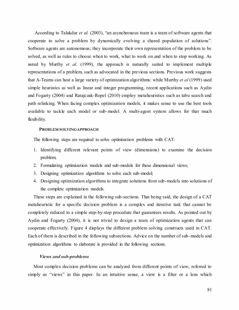
81
According to Talukdar et al. (2003), “an asynchronous team is a team of software agents that
cooperate to solve a problem by dynamically evolving a shared population of solutions”.
Software agents are autonomous; they incorporate their own representation of the problem to be
solved, as well as rules to choose when to work, what to work on and when to stop working. As
noted by Murthy et al. (1999), the approach is naturally suited to implement multiple
representations of a problem, such as advocated in the previous sections. Previous work suggests
that A-Teams can host a large variety of optimization algorithms: while Murthy et al (1999) used
simple heuristics as well as linear and integer programming, recent applications such as Aydin
and Fogarty (2004) and Ratajczak-Ropel (2010) employ metaheuristics such as tabu search and
path relinking. When facing complex optimization models, it makes sense to use the best tools
available to tackle each model or sub-model. A multi-agent system allows for that much
flexibility.
PROBLEM SOLVING APPROACH
The following steps are required to solve optimization problems with CAT:
1. Identifying different relevant points of view (dimensions) to examine the decision
problem;
2. Formulating optimization models and sub-models for these dimensional views;
3. Designing optimization algorithms to solve each sub-model;
4. Designing optimization algorithms to integrate solutions from sub-models into solutions of
the complete optimization models.
These steps are explained in the following sub-sections. That being said, the design of a CAT
metaheuristic for a specific decision problem is a complex and iterative task that cannot be
completely reduced to a simple step-by-step procedure that guarantees results. As pointed out by
Aydin and Fogarty (2004), it is not trivial to design a team of optimization agents that can
cooperate effectively. Figure 4 displays the different problem solving constructs used in CAT.
Each of them is described in the following subsections. Advice on the number of sub-models and
optimization algorithms to elaborate is provided in the following sections.
Views and sub-problems
Most complex decision problems can be analyzed from different points of view, referred to
simply as “views” in this paper. In an intuitive sense, a view is a filter or a lens which
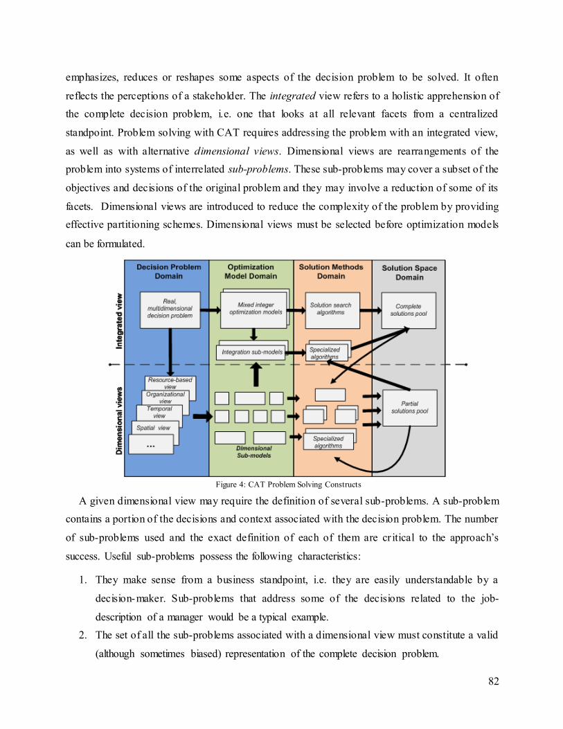
82
emphasizes, reduces or reshapes some aspects of the decision problem to be solved. It often
reflects the perceptions of a stakeholder. The integrated view refers to a holistic apprehension of
the complete decision problem, i.e. one that looks at all relevant facets from a centralized
standpoint. Problem solving with CAT requires addressing the problem with an integrated view,
as well as with alternative dimensional views. Dimensional views are rearrangements of the
problem into systems of interrelated sub-problems. These sub-problems may cover a subset of the
objectives and decisions of the original problem and they may involve a reduction of some of its
facets. Dimensional views are introduced to reduce the complexity of the problem by providing
effective partitioning schemes. Dimensional views must be selected before optimization models
can be formulated.
Figure 4: CAT Problem Solving Constructs
A given dimensional view may require the definition of several sub-problems. A sub-problem
contains a portion of the decisions and context associated with the decision problem. The number
of sub-problems used and the exact definition of each of them are cr itical to the approach’s
success. Useful sub-problems possess the following characteristics:
1. They make sense from a business standpoint, i.e. they are easily understandable by a
decision-maker. Sub-problems that address some of the decisions related to the job-
description of a manager would be a typical example.
2. The set of all the sub-problems associated with a dimensional view must constitute a valid
(although sometimes biased) representation of the complete decision problem.
83
In the context of the location-routing problem, the following two dimensional views could be
defined:
A functional view associated with the types of decisions (location, customer allocation to
facilities, and vehicle routing) associated with the decision problem. The problem can then
be partitioned into a DC location sub-problem, a customer-to-DC allocation sub-problem,
and a transportation or route design sub-problem.
As with most location problems, the LRP has an inherent spatial dimension. Indeed, the
customer base served by a company may cover a large territory, and logistics decisions
may be made on a national or sales region level instead of globally. In this context, the
problem can be partitioned into several regional sub-problems.
These dimensions and the associated sub-problems are easily understandable by a decision-
maker. Furthermore, each regional sub-problem contains all decision types, and each functional
sub-problem contains decisions for all regions. Consequently, they both constitute a valid
representation of the whole problem.
Models and sub-models
The integrated view leads to the formulation of a ‘complete’ optimization model to represent
the decision problem. This model is generally very difficult to solve, but it will be used for a
number of purposes. Variants of this model may also be formulated. For each dimensional view,
sub-models are formulated to represent sub-problems. These formulations are usually expressed
in terms of partitions of complete model decision variable vectors and parameter matrices. They
may also be based on alternative modeling formalisms: for example, a constraint programming
sub-model could be defined even if the complete optimization model is a mixed-integer program
(MIP). A sub-model is useful if it can be solved efficiently. This will usually be the case if the
sub-model:
Corresponds to a generic class of decision models studied in depth in the literature (ex:
knapsack, bin packing, graph coloring, traveling salesman, facility location models);
Can be solved to optimality using generic LP-MIP solvers, or dynamic programming, or
simple enumeration (explicit or implicit);
Isolates a homogeneous group of binary/integer variables and their associated constraints.
84
Optimization algorithms
Once the sub-models have been formulated, optimization algorithms must be designed to
solve them. In CAT, optimization algorithms are implemented as a set of autonomous software
agents. Solutions to sub-models are recorded and subsequently used to build complete solutions.
The following guidelines may be useful to select a solution method:
Developing greedy heuristics or GRASP (Feo and Resende, 1989) metaheuristics to
construct feasible solutions for profit maximizing or cost minimizing sub-models is
usually straightforward;
When the sub-models has been studied in the literature, published solution methods or
available code can be integrated into CAT;
Purely linear sub-models can be solved using a LP-solver library;
Sub-models involving a homogeneous group of binary/integer variables can usually be
solved effectively with a local search metaheuristic since it is rather straightforward to
define a neighborhood in this context.
In the LRP context, for example, some of the sub-models formulated and the solution methods
selected could be the following:
A pure facility location sub-model solved wits a MIP solver such as CPLEX;
A location-allocation sub-model solved with a Lagrangean heuristic (Beasley 1993);
A vehicle routing sub-model solved with a tabu search heuristic (Cordeau and Laporte
2005);
A regional LRP sub-model solved with a tabu search / simulated annealing hybrid (Wu et
al. 2002).
Integration sub-models
Solving dimensional sub-models is necessary but not sufficient for a successful CAT
implementation. Integration refers to combining the solutions of the sub-models associated with
one dimensional view into solutions to the complete optimization model. This is done by solving
an integration sub-model heuristically or with exact methods. Integration sub-models are
essentially restricted versions of the complete optimization model obtained by fixing the value of
several decision variables. The fixed values are provided by the solutions to the dimensional sub-
models. By solving the integration sub-model, the optimal value of the non-fixed decision
variables is found, and a solution to the complete optimization model is produced. We refer to the
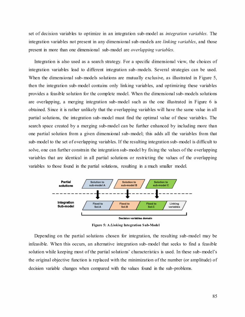
85
set of decision variables to optimize in an integration sub-model as integration variables. The
integration variables not present in any dimensional sub-models are linking variables, and those
present in more than one dimensional sub-model are overlapping variables.
Integration is also used as a search strategy. For a specific dimensional view, the choices of
integration variables lead to different integration sub-models. Several strategies can be used.
When the dimensional sub-models solutions are mutually exclusive, as illustrated in Figure 5,
then the integration sub-model contains only linking variables, and optimizing these variables
provides a feasible solution for the complete model. When the dimensional sub-models solutions
are overlapping, a merging integration sub-model such as the one illustrated in Figure 6 is
obtained. Since it is rather unlikely that the overlapping variables will have the same value in all
partial solutions, the integration sub-model must find the optimal value of these variables. The
search space created by a merging sub-model can be further enhanced by including more than
one partial solution from a given dimensional sub-model; this adds all the variables from that
sub-model to the set of overlapping variables. If the resulting integration sub-model is difficult to
solve, one can further constrain the integration sub-model by fixing the values of the overlapping
variables that are identical in all partial solutions or restricting the values of the overlapping
variables to those found in the partial solutions, resulting in a much smaller model.
Figure 5: A Linking Integration Sub-Model
Depending on the partial solutions chosen for integration, the resulting sub-model may be
infeasible. When this occurs, an alternative integration sub-model that seeks to find a feasible
solution while keeping most of the partial solutions’ characteristics is used. In these sub-model’s
the original objective function is replaced with the minimization of the number (or amplitude) of
decision variable changes when compared with the values found in the sub-problems.
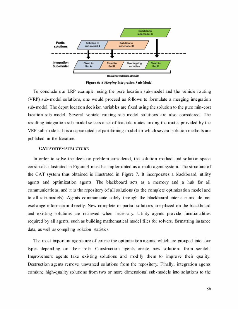
86
Figure 6: A Merging Integration Sub-Model
To conclude our LRP example, using the pure location sub-model and the vehicle routing
(VRP) sub-model solutions, one would proceed as follows to formulate a merging integration
sub-model. The depot location decision variables are fixed using the solution to the pure min-cost
location sub-model. Several vehicle routing sub-model solutions are also considered. The
resulting integration sub-model selects a set of feasible routes among the routes provided by the
VRP sub-models. It is a capacitated set partitioning model for which several solution methods are
published in the literature.
CAT SYSTEM STRUCTURE
In order to solve the decision problem considered, the solution method and solution space
constructs illustrated in Figure 4 must be implemented as a multi-agent system. The structure of
the CAT system thus obtained is illustrated in Figure 7. It incorporates a blackboard, utility
agents and optimization agents. The blackboard acts as a memory and a hub for all
communications, and it is the repository of all solutions (to the complete optimization model and
to all sub-models). Agents communicate solely through the blackboard interface and do not
exchange information directly. New complete or partial solutions are placed on the blackboard
and existing solutions are retrieved when necessary. Utility agents provide functionalities
required by all agents, such as building mathematical model files for solvers, formatting instance
data, as well as compiling solution statistics.
The most important agents are of course the optimization agents, which are grouped into four
types depending on their role. Construction agents create new solutions from scratch.
Improvement agents take existing solutions and modify them to improve their quality.
Destruction agents remove unwanted solutions from the repository. Finally, integration agents
combine high-quality solutions from two or more dimensional sub-models into solutions to the
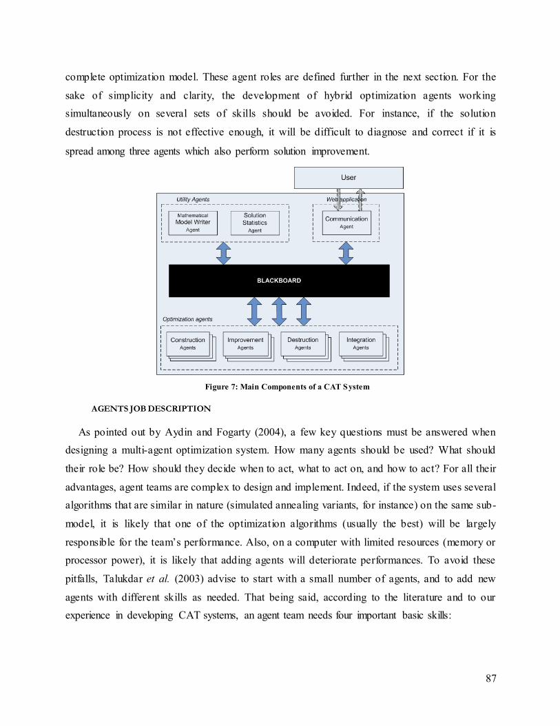
87
complete optimization model. These agent roles are defined further in the next section. For the
sake of simplicity and clarity, the development of hybrid optimization agents working
simultaneously on several sets of skills should be avoided. For instance, if the solution
destruction process is not effective enough, it will be difficult to diagnose and correct if it is
spread among three agents which also perform solution improvement.
Figure 7: Main Components of a CAT System
AGENTS JOB DESCRIPTION
As pointed out by Aydin and Fogarty (2004), a few key questions must be answered when
designing a multi-agent optimization system. How many agents should be used? What should
their role be? How should they decide when to act, what to act on, and how to act? For all their
advantages, agent teams are complex to design and implement. Indeed, if the system uses several
algorithms that are similar in nature (simulated annealing variants, for instance) on the same sub-
model, it is likely that one of the optimization algorithms (usually the best) will be largely
responsible for the team’s performance. Also, on a computer with limited resources (memory or
processor power), it is likely that adding agents will deteriorate performances. To avoid these
pitfalls, Talukdar et al. (2003) advise to start with a small number of agents, and to add new
agents with different skills as needed. That being said, according to the literature and to our
experience in developing CAT systems, an agent team needs four important basic skills:
88
1. Quickly obtain feasible solutions to the complete optimization model. Although these may
not be of high quality, they provide a basis for other agents to work upon.
2. Improve existing solutions. This can be done at the complete model level or agents ca n
work on specific parts of the problem.
3. Remove unwanted or poor solutions from the population to control its size.
4. Efficiently combine features from solutions originating from different methods or
dimensions.
The nature of these skills is discussed in the following sub-sections.
Generating an initial solution using construction agents
Feasible solutions can be obtained easily and quickly with simple heuristics, greedy
algorithms, hill-climbing procedures, or even by random generation, for several classes of
optimization models. Another option is to use generic LP / MIP heuristics such as feasibility
pump variants (Achterberg and Berthold, 2007); this approach tends to produce solutions that are
very different than those obtained with greedy methods and other heuristics. The key goals at this
task are speed and diversity, rather than solution quality. Using a variety of methods usually
results in a more diverse initial population of solutions, yielding a higher potential for
improvement and collaboration, and reducing the need for specific diversification strategies. If
the complete optimization model is difficult to solve but it is easy to find a feasible solution, one
can generate solutions to the complete model then infer initial solutions for sub-models from
these solutions, thus reducing the number of algorithms and agents needed for this role.
Evolving the solution population using improvement agents
For complex decision problems, it is recommended to work on sub-models rather than on the
complete model. Since defining a single neighborhood (or even a set of neighborhoods covering
the complete model’s range of variables) may be very challenging, local search is typically
difficult to use. Evolutionary computing provides generic crossover operators, but so lution
encoding is complex and on highly constrained problems, developing effective repair functions
may be problematic. In order to design a good set of improvement agents, the solution methods
used to solve sub-models must be carefully selected. As indicated previously, if the sub-model is
a linear program then existing LP-solvers can be used; if it has only one type of binary / integer
variable – allowing for the construction of neighborhoods – then a local search metaheuristic
89
(tabu search, VNS, …) can be developed; if it is a variant of a well-studied problem, the best
available method can be implemented. It may also be worthy to investigate alternative sub-model
reformulations.
A number of strategies can be used to tackle complex sub-models. For instance, an initial
solution obtained with a simple heuristic may provide a hot-start for a MIP-solver. Nowadays,
commercial solvers incorporate several generic MIP heuristic algorithms such as RINS (Danna et
al. 2005) or local branching (Fischetti and Lodi 2003). When metaheuristics are not efficient,
generic MIP heuristics often are. Ball (2011) provides an interesting review of heuristics based on
mathematical programming.
To ensure that the system continuously works on each sub-model (or, at least, looks for
opportunities to work on it), a dedicated agent should be assigned to its solution. The creation of
“super-agents” performing several tasks should be avoided. Such super-agents tend to use too
much resource and require complex scheduling rules. As will be shown, simple triggers are easier
to manage than complex ones.
Removing poor solutions using a destruction agent
According to Talukdar et al. (2003), solution destruction is as important as solution creation in
agent-based optimization. In some situations, the choice of solutions to destroy is obvious, such
as when duplicates exist in the population. Aside from maintaining some control over the size of
the population, destruction serves two purposes: removing poor quality solutions as well as
maintaining diversity in terms of solution characteristics. At the beginning of the search, the
solutions in the population are quite diverse. As improvement agents work, the solution quality of
the best solutions in the population improves rapidly. At this s tage, the destruction agent should
focus on removing solutions that are of poor quality. A simple rule such as choosing a solution at
random from those in the 4th quartile in terms of solution quality is appropriate.
However, as the overall quality of solution improves, newly created solutions tend not to be
competitive in terms of solution quality compared to those which have been improved by several
agents. They should have a chance to be improved before they are discarded. Furthermore, as the
population improves, working on the same solutions tends to accelerate convergence. As the
search progresses, a destruction agent shifts its focus from removing poor solutions to either:
90
Removing a random solution which has been improved at least (X – 2) times and is in the
bottom half in terms of performance, where X is the number of improvements made on the
solution that has been improved most frequently in the population;
Finding the two solutions in the population that are most similar, and then destroying the
worst one;
Finding the solution which has been used the most frequently to create new solutions
among the solutions in the 4th quartile in terms of solution quality, and destroying it.
These rules can be encapsulated in one or more destruction agents, and they work equally well
on a population of complete solutions or on a population of partial solutions (solutions to a
specific sub-problem). The two metrics necessary to implement them are detailed in the
following sections. Alternatively, some solutions can be “protected” and be immune to deletion
for a certain amount of time. These solutions may be the statu quo or solutions provided by a
decision-maker.
Amalgamation and diversification using integration agents
In our experience, CAT performs better when the population of solutions maintains a high
level of diversity. Although the destruction agent works toward maintaining variety, additional
diversification strategies may be needed. It is possible to add an agent whose sole objective is to
provide the population with radically different solutions than those currently in the population.
This agent should maintain a record of what has been proposed in the past, so it does not produce
solutions similar to those already removed from the population due to poor so lution quality. Two
examples of diversification agents are outlined in the application section.
The integration of partial solutions from sub-models into complete solutions is a key
component of an efficient agent team. At least one optimization algorithm should be provided for
each integration sub-model. If two methods are readily available, they can both be used if they
generate different high quality solutions. The number of actual agents to use depends on the
relative speed at which the improvement agents generate new solutions to sub-models and the
amount of computation effort required to solve the integration sub-models.
Integration can be used in very flexible ways. Integration of solutions to sub-models from
different dimensional views can be desirable, as long as the resulting merging integration sub-
models are not exceedingly difficult to solve. Solving these models often require the design of
91
specific heuristics or the use of a generic heuristic such as local branching (Fischetti and Lodi,
2003) or RINS (Danna et al. 2005). These heuristic are easily implemented using a MIP solver
such as CPLEX or Gurobi. This approach is in line with scatter search and path-relinking
metaheuristics and is an effective way of reaping the most benefits from using multiple
dimensional views. As this type of integration is slightly different than the type of integration
sub-models required to assemble complete solutions from partial solutions, these sub-models
should be assigned to a different integration agent.
DECISION RULES AND METRICS
In order to complete its job description, an agent needs formal rules to determine which
solution to work on. A trivial option is to select a random solution from the population, but this
does not give very good results. Obviously, an agent does not want to select a solution that it has
recently worked on. A simple yet effective decision rule is that the agent waits that at least three
others agents have improved the solution before attempting to work on it again. Some
improvement agents such as local search metaheuristics may want to push that rule a little
further: since a local search heuristic explores thoroughly a restricted portion of the search space
(Gendreau and Potvin 2010), an agent may want to select a solution that is significantly different
than the one it just worked on. In order to design more sophisticated decision rules, a few metrics
must be computed and are described below.
Solution ancestry
Agents need an effective way to determine which solutions they recently worked on. In a
cooperative context, this information should be accessible to all agents. A simple metric to
achieve this objective is solution’s ancestry. Simply put, a solution’s ancestry is its genealogical
tree. Each solution keeps track of the solutions used for its creation, or as a basis for its
improvement, as well as the agents that worked on it. An improvement agent can then use this
information to determine whether it has worked on a solution recently, or on any of its parents.
Tied to each solution is a list of agents that have worked on the solution, and whether this attempt
at improving the solution succeeded or not. This list is sorted in reverse order. A similar
mechanism is used to determine whether or not a solution has transmitted its characteristics to
other solutions in the population. Anytime a solution is used to create a new solution or to alter
an existing solution, its characteristics are propagated through the population. The new solution is
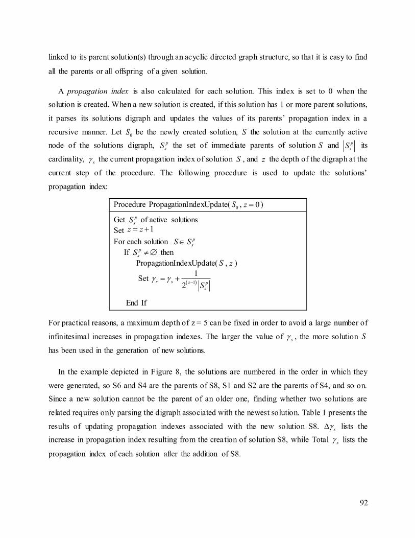
92
linked to its parent solution(s) through an acyclic directed graph structure, so that it is easy to find
all the parents or all offspring of a given solution.
A propagation index is also calculated for each solution. This index is set to 0 when the
solution is created. When a new solution is created, if this solution has 1 or more parent solutions,
it parses its solutions digraph and updates the values of its parents’ propagation index in a
recursive manner. Let 0S be the newly created solution, S the solution at the currently active
node of the solutions digraph, p
sS the set of immediate parents of solution S and p
sS its
cardinality, s the current propagation index of solution S , and z the depth of the digraph at the
current step of the procedure. The following procedure is used to update the solutions’
propagation index:
Procedure PropagationIndexUpdate(0S , 0z )
Get p
sS of active solutions
Set 1z z
For each solution p
sS S
If p
sS then
PropagationIndexUpdate( S , z )
Set 1
1
2s s z p
sS
End If
For practical reasons, a maximum depth of z = 5 can be fixed in order to avoid a large number of
infinitesimal increases in propagation indexes. The larger the value of s , the more solution S
has been used in the generation of new solutions.
In the example depicted in Figure 8, the solutions are numbered in the order in which they
were generated, so S6 and S4 are the parents of S8, S1 and S2 are the parents of S4, and so on.
Since a new solution cannot be the parent of an older one, finding whether two solutions are
related requires only parsing the digraph associated with the newest solution. Table 1 presents the
results of updating propagation indexes associated with the new solution S8. s lists the
increase in propagation index resulting from the creation of solution S8, while Total s lists the
propagation index of each solution after the addition of S8.
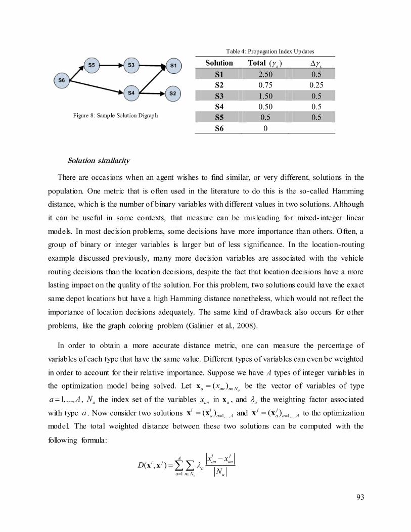
93
Table 4: Propagation Index Updates
Solution Total ( )s s
S1 2.50 0.5
S2 0.75 0.25
S3 1.50 0.5
S4 0.50 0.5
S5 0.5 0.5
S6 0
Solution similarity
There are occasions when an agent wishes to find similar, or very different, solutions in the
population. One metric that is often used in the literature to do this is the so-called Hamming
distance, which is the number of binary variables with different values in two solutions. Although
it can be useful in some contexts, that measure can be misleading for mixed- integer linear
models. In most decision problems, some decisions have more importance than others. Often, a
group of binary or integer variables is larger but of less significance. In the location-routing
example discussed previously, many more decision variables are associated with the vehicle
routing decisions than the location decisions, despite the fact that location decisions have a more
lasting impact on the quality of the solution. For this problem, two solutions could have the exact
same depot locations but have a high Hamming distance nonetheless, which would not reflect the
importance of location decisions adequately. The same kind of drawback also occurs for other
problems, like the graph coloring problem (Galinier et al., 2008).
In order to obtain a more accurate distance metric, one can measure the percentage of
variables of each type that have the same value. Different types of variables can even be weighted
in order to account for their relative importance. Suppose we have A types of integer variables in
the optimization model being solved. Let ( )aa an n Nx x
be the vector of variables of type
1,...,a A , aN the index set of the variables anx in ax , and a the weighting factor associated
with type a . Now consider two solutions 1,...,( )i i
a a Ax x and 1,...,( )j j
a a Ax x to the optimization
model. The total weighted distance between these two solutions can be computed with the
following formula:
1
( , )a
i jA
an ani j
a
a n N a
x xD
N
x x
Figure 8: Sample Solution Digraph

94
4.2.5 Experimental test case
This section provides an experimental test case to illustrate how CAT can be applied to solve a
specific complex decision problem, and to demonstrate the validity and the effectiveness of the
approach. More specifically, we show how to use CAT to solve multi-period Supply Chain
Network (SCN) design problems.
4.2.5.1 Multi-Period Supply Chain Network Design Model
According to Santoso et al. (2005), SCN design is a crucial component of the planning
activities of today’s world-class manufacturing firms. As Klibi et al. (2010) point out, typical
SCN design problems involves strategic decisions on the number, location, capacity and missions
of the production-distribution facilities a company should use to provide goods to a set of
potential product-markets. A large number of particular formulations and solution methods have
been proposed for single and multi-period versions of the SCN design problem, such as Vidal and
Goetschalckx (2001), Paquet et al. (2004) and Martel (2005); the latter also provides an extensive
overview of the relevant literature.
SCN design decisions are revised at the beginning of a set N of reengineering cycles each
covering one or several planning periods nt T n N , . Collectively, these reengineering cycles
define the planning horizon n N nT T . Under the assumption that the future is known with
certainty, the structure of the mathematical programming model to solve on a rolling horizon
basis, for the prevailing SCN design paradigm, can be synthesized as follows. The following
notation is used.
p
nx : Vector of binary decision variables equal to 1 when using a given facility platform on a
network site during reengineering cycle n N .
s
nx : Vector of binary decision variables equal to 1 when a given sourcing/transportation
contract is selected for reengineering cycle n N .
d
nx : Vector of binary decision variables equal to 1 when a given demand shaping offer is
selected for a product-market during reengineering cycle n N .
p s d( , , )n n n nx x x x : Vector of all binary design variables for cycle n N .
f
ty : Vector of aggregate product flows on the network arcs in planning period t T .
a
ty : Vector of aggregate activity levels (production or throughput) in the nodes (plants or
depots) of the network in planning period t T .
95
i
ty : Vector of aggregate inventory levels in the nodes of the network at the end of planning
period t T .
f a i( , , )t t t ty y y y : Vector of all continuous activity level variables for period t T .
f
tp : Vector of the unit prices paid for the delivery of the products associated with the flows f
ty
.
tc : Vector of the unit variable costs associated with the elements of activity vector ty .
te : Vector of the capital recovery or contract expenditures in planning period t for the
elements of design vector ( )n tx (n(t) denotes the cycle n including planning period t).
tEVA : Economic value added by the SCN in planning period t T .
: Discount rate used by the company, based on its weighted average cost of capital
(WACC).
c
tb : Vector of the capacity provided in period t T by the platform, sourcing and
transportation resources/contracts associated with the elements of design vector p s
( ) ( )( , )n t n tx x .
d
tb : Vector of the potential demand available in period t T under the demand-shaping offer
associated with the elements of design vector ( )
d
n tx .
c d( , )t t tb b b : Vector of all capability parameter values associated with design vector ( )n tx for
period t T .
In these definitions, platforms refer to alternative facility resource configurations that can be
implemented on a site. They are characterized by technology and capacity choices to support a
set of activities, and they involve specified capital recovery expenditures. A site without platform
is not utilized. The platform on a site can change at the beginning of reengineering cycles to
reflect opening, closing, expansion or reorganization decisions. Platforms are also used to
characterize the proposals of potential subcontractors or public warehouses. In some
formulations, complementary change-of-state binary variables are defined to facilitate the
modeling of implementation expenses. Sourcing and transportation contracts specify prices and
capacity for raw material and transportation service vendors. Demand-shaping offers are potential
product-market selling policies specified in terms of price, response time, fill rate, or other order
winning criterion. They influence demand and they may impose constraints on the network
structure. Individual products daily/weekly procurement, production, inventory and shipping
decisions are aggregated into flow, activity level and inventory level decisions for product
families, demand zones and planning periods.
96
Using this notation, a typical multi-period SCN design model can be formulated as follows:
f f
( )max , [ ]
(1 )
tt t t t t t n tt
t T
EVAEVA
p y c y e x (1)
subject to
p p
1 1n n n n n V x W x u (2)
n nXx (3)
( )t t t n tA y b x
(4)
1( , )
t t tY
y y
(5)
where 1n
V , n
W and t
A are parameter matrices, n
u is a parameter vector, nX is the set o f
feasible designs specified by local cycle n constraints, and t
Y is an activity level feasibility set for
planning period t. The objective function (1) maximizes value creation over the planning horizon.
Constraints (2) ensure that platforms are changed coherently from a reengineering cycle ( p
1nx ) to
the next ( p
nx ). Constraints (3) include additional cycle dependent constraints required to make
sure that design options are properly selected. For example, during a cycle, one cannot operate
more than one platform on a site or select more than one demand shaping offer for a product-
market. Constraints (4) specify the activity level restrictions imposed in period t T by the
capabilities provided by the selected design ( )n tx . These are mainly production-warehousing
capacity constraints on a
ty , storage capacity constraints on i
ty , as well as vendor capacity,
transportation capacity and potential demand constraints on f
ty . Finally, (5) includes mainly flow
conservation constraints on ty , and accounting constraints to calculate end-of-period inventories i
ty from initial inventories i
1ty and relevant inflows/outflows in f a( , )t ty y .
This streamlined formulation captures the main elements of multi-cycles SCN design models
such as those proposed by Martel (2005), Thanh et al. (2010), and Carle et al. (2012). The model
provided above is general and conceptual; a particular implementation may need some extra
constraints imposing operational limits, such as maximum number of facilities to be built or
expanded per planning cycle. The exact problem formulation used for the experimental tests,
along with a detailed discussion of modeling choices, is provided in Carle et al. (2012).
4.2.5.2 CAT Implementation
In the SCN design problem examined, three dimensional views were adopted to identify sub-
problems and formulate associated sub-models. Each one is closely connected to the nature of the
decision problem to be solved and to its mathematical formulation. Figure 9 presents these
n N
n N
t T
t T
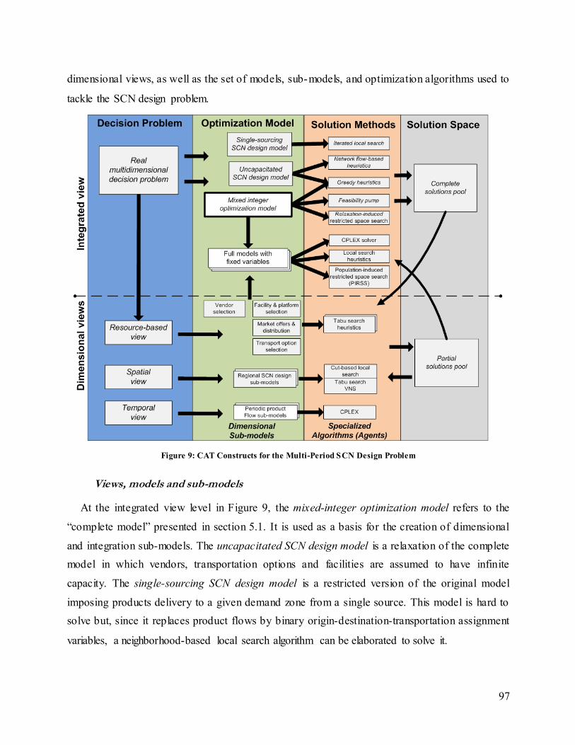
97
dimensional views, as well as the set of models, sub-models, and optimization algorithms used to
tackle the SCN design problem.
Figure 9: CAT Constructs for the Multi-Period SCN Design Problem
Views, models and sub-models
At the integrated view level in Figure 9, the mixed-integer optimization model refers to the
“complete model” presented in section 5.1. It is used as a basis for the creation of dimensional
and integration sub-models. The uncapacitated SCN design model is a relaxation of the complete
model in which vendors, transportation options and facilities are assumed to have infinite
capacity. The single-sourcing SCN design model is a restricted version of the original model
imposing products delivery to a given demand zone from a single source. This model is hard to
solve but, since it replaces product flows by binary origin-destination-transportation assignment
variables, a neighborhood-based local search algorithm can be elaborated to solve it.
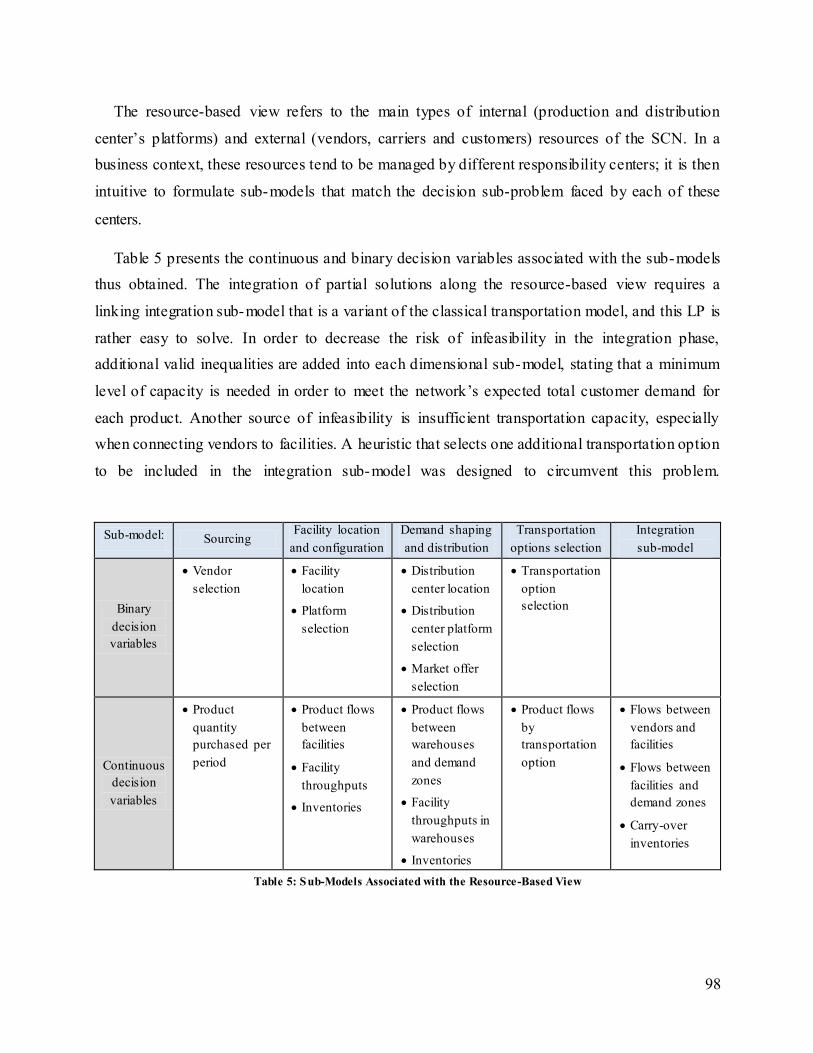
98
The resource-based view refers to the main types of internal (production and distribution
center’s platforms) and external (vendors, carriers and customers) resources of the SCN. In a
business context, these resources tend to be managed by different responsibility centers; it is then
intuitive to formulate sub-models that match the decision sub-problem faced by each of these
centers.
Table 5 presents the continuous and binary decision variables associated with the sub-models
thus obtained. The integration of partial solutions along the resource-based view requires a
linking integration sub-model that is a variant of the classical transportation model, and this LP is
rather easy to solve. In order to decrease the risk of infeasibility in the integration phase,
additional valid inequalities are added into each dimensional sub-model, stating that a minimum
level of capacity is needed in order to meet the network’s expected total customer demand for
each product. Another source of infeasibility is insufficient transportation capacity, especially
when connecting vendors to facilities. A heuristic that selects one additional transportation option
to be included in the integration sub-model was designed to circumvent this problem.
Sub-model: Sourcing Facility location
and configuration
Demand shaping
and distribution
Transportation
options selection
Integration
sub-model
Binary
decision
variables
Vendor
selection
Facility
location
Platform
selection
Distribution
center location
Distribution
center platform
selection
Market offer
selection
Transportation
option
selection
Continuous
decision
variables
Product
quantity
purchased per
period
Product flows
between
facilities
Facility
throughputs
Inventories
Product flows
between
warehouses
and demand
zones
Facility
throughputs in
warehouses
Inventories
Product flows
by
transportation
option
Flows between
vendors and
facilities
Flows between
facilities and
demand zones
Carry-over
inventories
Table 5: Sub-Models Associated with the Resource-Based View
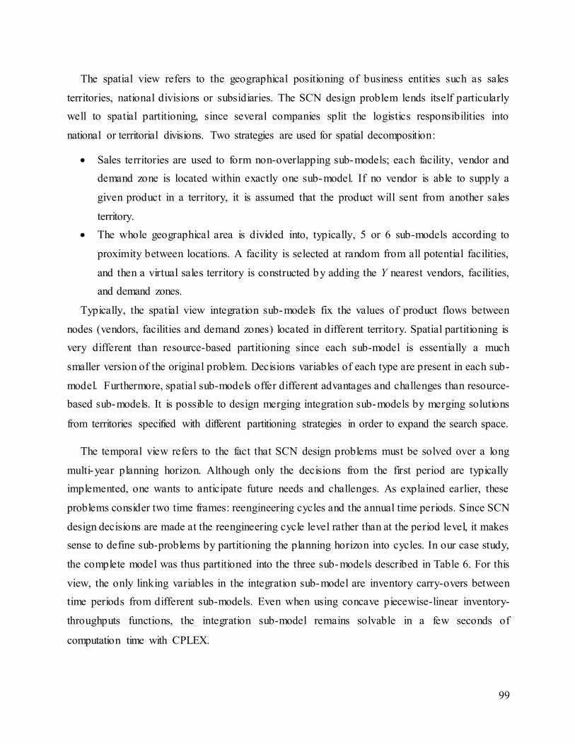
99
The spatial view refers to the geographical positioning of business entities such as sales
territories, national divisions or subsidiaries. The SCN design problem lends itself particularly
well to spatial partitioning, since several companies split the logistics responsibilities into
national or territorial divisions. Two strategies are used for spatial decomposition:
Sales territories are used to form non-overlapping sub-models; each facility, vendor and
demand zone is located within exactly one sub-model. If no vendor is able to supply a
given product in a territory, it is assumed that the product will sent from another sales
territory.
The whole geographical area is divided into, typically, 5 or 6 sub-models according to
proximity between locations. A facility is selected at random from all potential facilities,
and then a virtual sales territory is constructed by adding the Y nearest vendors, facilities,
and demand zones.
Typically, the spatial view integration sub-models fix the values of product flows between
nodes (vendors, facilities and demand zones) located in different territory. Spatial partitioning is
very different than resource-based partitioning since each sub-model is essentially a much
smaller version of the original problem. Decisions variables of each type are present in each sub-
model. Furthermore, spatial sub-models offer different advantages and challenges than resource-
based sub-models. It is possible to design merging integration sub-models by merging solutions
from territories specified with different partitioning strategies in order to expand the search space.
The temporal view refers to the fact that SCN design problems must be solved over a long
multi-year planning horizon. Although only the decisions from the first period are typically
implemented, one wants to anticipate future needs and challenges. As explained earlier, these
problems consider two time frames: reengineering cycles and the annual time periods. Since SCN
design decisions are made at the reengineering cycle level rather than at the period level, it makes
sense to define sub-problems by partitioning the planning horizon into cycles. In our case study,
the complete model was thus partitioned into the three sub-models described in Table 6. For this
view, the only linking variables in the integration sub-model are inventory carry-overs between
time periods from different sub-models. Even when using concave piecewise-linear inventory-
throughputs functions, the integration sub-model remains solvable in a few seconds of
computation time with CPLEX.
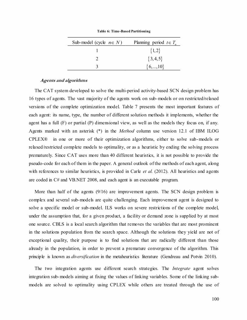
100
Table 6: Time-Based Partitioning
Sub-model (cycle n N ) Planning period nt T
1 1,2
2 3,4,5
3 6,...,10
Agents and algorithms
The CAT system developed to solve the multi-period activity-based SCN design problem has
16 types of agents. The vast majority of the agents work on sub-models or on restricted/relaxed
versions of the complete optimization model. Table 7 presents the most important features of
each agent: its name, type, the number of different solution methods it implements, whether the
agent has a full (F) or partial (P) dimensional view, as well as the models they focus on, if any.
Agents marked with an asterisk (*) in the Method column use version 12.1 of IBM ILOG
CPLEX® in one or more of their optimization algorithms, either to solve sub-models or
relaxed/restricted complete models to optimality, or as a heuristic by ending the solving process
prematurely. Since CAT uses more than 40 different heuristics, it is not possible to provide the
pseudo-code for each of them in the paper. A general outlook of the methods of each agent, along
with references to similar heuristics, is provided in Carle et al. (2012). All heuristics and agents
are coded in C# and VB.NET 2008, and each agent is an executable program.
More than half of the agents (9/16) are improvement agents. The SCN design problem is
complex and several sub-models are quite challenging. Each improvement agent is designed to
solve a specific model or sub-model. ILS works on severe restrictions of the complete model,
under the assumption that, for a given product, a facility or demand zone is supplied by at most
one source. CBLS is a local search algorithm that removes the variables that are most prominent
in the solutions population from the search space. Although the solutions they yield are not of
exceptional quality, their purpose is to find solutions that are radically different than those
already in the population, in order to prevent a premature convergence of the algorithm. This
principle is known as diversification in the metaheuristics literature (Gendreau and Potvin 2010).
The two integration agents use different search strategies. The Integrate agent solves
integration sub-models aiming at fixing the values of linking variables. Some of the linking sub-
models are solved to optimality using CPLEX while others are treated through the use of
101
heuristics. Since the improvement agents produce a large quantity of partial solutions, the speed
of the integration process is of prime importance. As such, it would be impractical, both in terms
of computation time and RAM, to solve each integration sub-problem to optimality. In contrast,
the PIRSS agent focuses on merging integration sub-models. It effectively models the solution
space formed by the union of two or more solutions as a restricted MIP, and then explores it
thoroughly within a time limit using CPLEX. For instance, partial solutions from the sub-models
of the resource-based dimension are merged with a partial solution from a spatial sub-model.
Table 7: CAT Agents Implemented to Solve the SCN Design Problem
In our implementation, the destruction agent starts to remove solutions from the population
when it reaches 50 complete solutions, or 15 partial solutions to any sub-model.
4.2.6 Computational results
In order to validate and assess the CAT problem solving approach, a set of 25 benchmark
problem instances were generated. The first 20 of these instances (labeled B-01 to B-20) are
based on a realistic case representing a typical B2B company manufacturing and selling products
through the United States. Product demands and prices, transportation costs as well as the fixed
Agent Type Method Functional Spatial Time Models
FPump C 6* F F F Complete model
Greedy C 8 F F F Complete model and
Uncapacitated SCN design model
RIRSS C 2* F F F Complete model
BasicNet C 3 P P F Facility location, network flow, transportation
model
TSV I 1 P F F Sourcing sub-model
TSI I 2 P F F Facility location and configuration sub-model
TSD I 1 P F F Demand shaping and distribution sub-model
TransOpt I 1 P F F Transportation option sub-model
RegionalTS I 2 F P F Regional SCN design sub-model
CBLS I 2* P P P Regional SCN design sub-model
FlowOpt I 2* F F P Period ic network flow, time d imension
linking model
CPLEX-SP I 1* F F F Complete model
ILS I 1 F F F Complete model
Terminator D 3 F F F None; archives bad solutions
Integrate T 7* F F F Integration sub-models
PIRSS T 2* F F F Integration sub-models
Agent types: C – Construction; I – Improvement; D – Destruction; T – Integration.
102
and variable costs of each platform, vendor offer and transportation options are randomly
generated, but are based on realistic parameter value ranges found in Ballou (1992). The
remaining 5 (labeled G-01 to G-05) are based on randomized values using a procedure similar to
the one described in Cordeau, Pasin and Solomon (2006) to generate low-capacity, high flow
magnitude instances.
The potential supply chain network comprises 9 to 18 potential production-distribution
facilities, 30 to 60 potential distribution centers, 100 to 300 demand zones representing clusters
of customers in the vicinity of major U.S. cities, and 50 to 300 vendor offers. For the production-
distribution facilities, 3 to 8 alternative platforms are considered, and up to 4 capacity expansion
upgrades are available for each of these platforms. For the distribution centers, 5 alternative
platforms are considered, with a maximum of 2 upgrades per platform. Five to 16 product
families are sold to customers, and their bill-of-materials include 10 to 60 components. Several
transport capacity options are modeled; truckload and less-than-truckload shipping are
considered, both in the form of a limited-size private fleet and long-term truck leasing. A
common carrier with a large capacity is also available. Five demand shaping offers are
considered for each product. All problem instances involve concave inventory-throughput
functions. When the models are solved with CPLEX, these concave functions are approximated
by 3-segments piecewise linear functions using a procedure similar to the one described in
Amrani et al. (2011). The resulting complete models each have millions of continuous variables
as well as from 20,000 to 200,000 binary variables. Note that this problem set is different than the
one used to validate the CAT system. This guarantees that the system is not custom-built or fine-
tuned for a given set of instances.
In order to assess the impact of the main CAT components on overall performance, three versions
of CAT were tested. The list of individual agents included in each version is provided in Table 8.
The “greedy” version contains the agents whose mission is to quickly generate several solutions
for the other agents to improve upon. The “basic version” contains all the agents found in the
greedy version as well as those built to tackle the dimensional sub-models, but it lacks any
sophisticated integration agent. The complete version contains the 16 agents listed in Table 7.
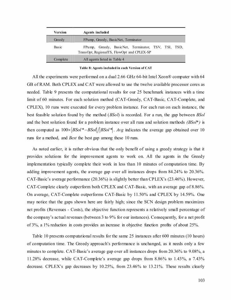
103
Table 8: Agents included in each Version of CAT
All the experiments were performed on a dual 2.66 GHz 64-bit Intel Xeon® computer with 64
GB of RAM. Both CPLEX and CAT were allowed to use the twelve available processor cores as
needed. Table 9 presents the computational results for our 25 benchmark instances with a time
limit of 60 minutes. For each solution method (CAT-Greedy, CAT-Basic, CAT-Complete, and
CPLEX), 10 runs were executed for every problem instance. For each run on each instance, the
best feasible solution found by the method (BSol) is recorded. For a run, the gap between BSol
and the best solution found for a problem instance over all runs and solution methods (BSol*) is
then computed as 100 * *BSol BSol BSol . Avg indicates the average gap obtained over 10
runs for a method, and Best the best gap among these 10 runs.
As noted earlier, it is rather obvious that the only benefit of using a greedy strategy is that it
provides solutions for the improvement agents to work on. All the agents in the Greedy
implementation typically complete their work in less than 10 minutes of computation time. By
adding improvement agents, the average gap over all instances drops from 84.24% to 20.36%.
CAT-Basic’s average performance (20.36%) is slightly better than CPLEX’s (23.46%). However,
CAT-Complete clearly outperform both CPLEX and CAT-Basic, with an average gap of 8.86%.
On average, CAT-Complete outperforms CAT-Basic by 11.50% and CPLEX by 14.59%. One
may notice that the gaps shown here are fairly high; since the SCN design problem maximizes
net profits (Revenues - Costs), the objective function represents a relatively small percentage of
the company’s actual revenues (between 3 to 9% for our instances). Consequently, for a net profit
of 3%, a 1% reduction in costs provides an increase in objective function profits of about 25%.
Table 10 presents computational results for the same 25 instances after 600 minutes (10 hours)
of computation time. The Greedy approach’s performance is unchanged, as it needs only a few
minutes to complete. CAT-Basic’s average gap over all instances drops from 20.36% to 9.08%, a
11.28% decrease, while CAT-Complete’s average gap drops from 8.86% to 1.43%, a 7.43%
decrease. CPLEX’s gap decreases by 10.25%, from 23.46% to 13.21%. These results clearly
Version Agents included
Greedy FPump, Greedy, BasicNet, Terminator
Basic FPump, Greedy, BasicNet, Terminator, TSV, TSI, TSD,
TransOpt, RegionalTS, FlowOpt and CPLEX-SP
Complete All agents listed in Table 4
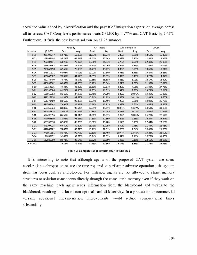
104
show the value added by diversification and the payoff of integration agents: on average across
all instances, CAT-Complete’s performance beats CPLEX by 11.77% and CAT-Basic by 7.65%.
Furthermore, it finds the best known solution on all 25 instances.
Table 9: Computational Results after 60 Minutes
It is interesting to note that although agents of the proposed CAT system use some
acceleration techniques to reduce the time required to perform read/write operations, the system
itself has been built as a prototype. For instance, agents are not allowed to share memory
structures or solution components directly through the computer’s memory even if they work on
the same machine; each agent reads information from the blackboard and writes to the
blackboard, resulting in a lot of non-optimal hard disk activity. In a production or commercial
version, additional implementation improvements would reduce computational times
substantially.
Instance (BSol*) Best Avg Best Avg Best Avg Best Avg
B-01 238798247 52.71% 59.93% 11.73% 18.24% 5.39% 7.86% 13.68% 15.37%
B-02 249367184 56.77% 65.47% 13.40% 20.54% 3.88% 6.80% 17.52% 19.25%
B-03 267302131 63.28% 75.02% 18.66% 24.84% 5.78% 7.50% 22.40% 25.95%
B-04 269632962 61.53% 76.14% 19.51% 24.76% 2.62% 6.89% 21.43% 24.02%
B-05 278667490 62.65% 76.19% 14.73% 19.47% 4.36% 6.95% 19.60% 19.84%
B-06 276510121 68.08% 79.02% 12.02% 17.50% 5.98% 8.53% 16.29% 18.26%
B-07 356662807 70.37% 84.12% 11.85% 18.03% 7.34% 9.48% 13.28% 14.37%
B-08 422735400 76.75% 86.07% 12.55% 18.88% 5.85% 8.99% 14.17% 18.60%
B-09 475093862 80.83% 87.83% 18.17% 25.54% 5.61% 7.89% 21.92% 26.81%
B-10 503154315 79.31% 86.29% 16.61% 22.67% 2.29% 4.96% 25.86% 27.75%
B-11 551335586 81.71% 87.95% 11.35% 16.31% 6.32% 9.80% 23.73% 25.54%
B-12 508660093 81.15% 87.97% 19.45% 24.70% 8.39% 10.96% 19.39% 19.82%
B-13 518215224 81.31% 87.58% 15.34% 21.82% 8.83% 10.11% 22.83% 24.75%
B-14 551371409 84.69% 90.38% 13.64% 19.49% 7.23% 9.81% 19.08% 20.73%
B-15 511565563 79.91% 84.37% 10.58% 15.92% 2.42% 5.60% 23.45% 24.47%
B-16 560355024 83.89% 90.54% 12.99% 19.61% 10.61% 13.27% 30.51% 31.00%
B-17 592086814 84.00% 90.16% 14.36% 21.44% 8.71% 10.72% 28.02% 30.96%
B-18 597498896 85.59% 91.01% 11.38% 18.01% 7.82% 10.01% 26.27% 28.52%
B-19 541063880 81.62% 91.11% 14.69% 22.39% 7.22% 9.66% 22.21% 25.37%
B-20 583337610 82.08% 86.76% 13.88% 19.78% 5.67% 8.19% 22.44% 23.63%
G-01 341707025 69.80% 80.29% 11.79% 17.95% 6.99% 9.45% 21.35% 21.98%
G-02 412869182 74.83% 85.72% 18.21% 22.81% 4.60% 7.04% 20.48% 21.96%
G-03 773059691 86.78% 90.77% 10.10% 15.46% 10.44% 12.46% 19.23% 22.99%
G-04 191659172 92.63% 98.69% 13.94% 22.02% 3.87% 9.46% 26.75% 31.40%
G-05 532929990 80.71% 86.54% 13.82% 20.80% 5.96% 9.16% 22.15% 23.07%
Average: 76.12% 84.24% 14.19% 20.36% 6.17% 8.86% 21.36% 23.46%
Greedy CAT-Basic CAT-Complete CPLEX
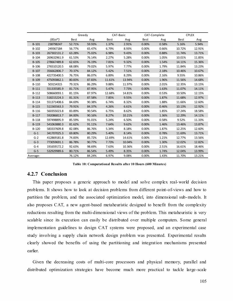
105
Table 10: Computational Results after 10 Hours (600 Minutes)
4.2.7 Conclusion
This paper proposes a generic approach to model and solve complex real-world decision
problems. It shows how to look at decision problems from different point-of-views and how to
partition the problem, and the associated optimization model, into dimensional sub-models. It
also proposes CAT, a new agent-based metaheuristic designed to benefit from the complexity
reductions resulting from the multi-dimensional views of the problem. This metaheuristic is very
scalable since its execution can easily be distributed over multiple computers. Some general
implementation guidelines to design CAT systems were proposed, and an experimental case
study involving a supply chain network design problem was presented. Experimental results
clearly showed the benefits of using the partitioning and integrat ion mechanisms presented
earlier.
Given the decreasing costs of multi-core processors and physical memory, parallel and
distributed optimization strategies have become much more practical to tackle large-scale
(BSol*) Best Avg Best Avg Best Avg Best Avg
B-101 238798247 52.71% 59.93% 1.37% 2.91% 0.00% 0.58% 5.16% 5.94%
B-102 249367184 56.77% 65.47% 6.79% 8.93% 0.00% 0.66% 10.72% 12.91%
B-103 267302131.2 63.28% 75.02% 6.98% 9.43% 0.00% 0.88% 11.74% 13.71%
B-104 269632961.9 61.53% 76.14% 2.27% 5.28% 0.00% 1.05% 10.01% 11.85%
B-105 278667489.8 62.65% 76.19% 7.81% 9.32% 0.00% 1.54% 14.11% 15.36%
B-106 276510120.5 68.08% 79.02% 5.97% 7.77% 0.00% 1.79% 11.84% 13.23%
B-107 356662806.7 70.37% 84.12% 5.42% 7.51% 0.00% 2.18% 10.46% 10.67%
B-108 422735400.5 76.75% 86.07% 6.89% 8.29% 0.00% 2.16% 9.55% 10.86%
B-109 475093862.1 80.83% 87.83% 11.61% 13.94% 0.00% 1.96% 11.56% 14.68%
B-110 503154315 79.31% 86.29% 9.88% 11.97% 0.00% 2.01% 12.35% 13.15%
B-111 551335585.9 81.71% 87.95% 5.47% 7.73% 0.00% 1.63% 11.07% 14.11%
B-112 508660093.1 81.15% 87.97% 12.68% 14.81% 0.00% 0.53% 10.50% 12.15%
B-113 518215224.3 81.31% 87.58% 7.85% 9.55% 0.00% 1.87% 11.68% 12.97%
B-114 551371408.6 84.69% 90.38% 6.74% 8.32% 0.00% 1.88% 11.66% 12.60%
B-115 511565563.3 79.91% 84.37% 4.26% 6.61% 0.00% 0.46% 10.13% 12.92%
B-116 560355023.8 83.89% 90.54% 6.75% 8.62% 0.00% 1.85% 17.24% 18.58%
B-117 592086813.7 84.00% 90.16% 8.27% 10.21% 0.00% 1.36% 12.29% 14.11%
B-118 597498895.9 85.59% 91.01% 5.24% 6.50% 0.00% 0.58% 9.52% 11.33%
B-119 541063880.3 81.62% 91.11% 7.64% 9.62% 0.00% 1.46% 13.46% 13.87%
B-120 583337609.8 82.08% 86.76% 5.34% 8.18% 0.00% 1.87% 12.25% 12.60%
G-1 341707025.3 69.80% 80.29% 5.40% 8.14% 0.00% 0.78% 11.69% 13.71%
G-2 412869181.8 74.83% 85.72% 12.69% 14.61% 0.00% 1.21% 12.77% 13.56%
G-3 773059691.1 86.78% 90.77% 7.73% 10.04% 0.00% 1.30% 12.02% 12.82%
G-4 191659172.2 92.63% 98.69% 7.63% 10.36% 0.00% 2.51% 16.61% 18.46%
G-5 532929989.6 80.71% 86.54% 5.49% 8.35% 0.00% 1.74% 12.04% 13.99%
Average: 76.12% 84.24% 6.97% 9.08% 0.00% 1.43% 11.70% 13.21%
Greedy CAT-Basic CAT-Complete CPLEX
106
decision problems. CAT is easily extendable by adding new agents or processing power as
needed or by allowing some of the agents to work using more than one processor at a time. A
more robust methodology to assess the impact and utility of a given agent could and should be
developed, in order to limit the number of agents used.
An interesting opportunity for further research is to apply CAT to other optimization models;
the location-routing and production- inventory-routing models seem promising, as are complex
production scheduling models. CAT should also be extended to model decision problems with
multiple decision makers, in cooperative or non-cooperative contexts. Another straightforward
extension would be to model multi- firm supply chain network design problems, where sub-
problems could be designed for the set of facilities owned by each participating firm. The agent
structure would enable the use of private information in the optimization sub-models without the
need to share such information with its supply chain partners.
4.2.8 References
[1] Achterberg T., Berthold T.; Improving the Feasibility Pump, Discrete Optimization, 4, 77-
86, 2007.
[2] Amrani H., Martel A., Zufferey N., Makeeva P.; A variable neighborhood search heuristic
for the design of multicommodity production-distribution networks with alternative facility
configuration, OR Spectrum, 33(4), 989-1007, 2011.
[3] Aydin M.E., Fogarty T.C.; Teams of autonomous agents for job-shop scheduling problems:
An experimental study, Journal of Intelligent Manufacturing, 15, 455-462, 2004.
[4] Balinski M., Fixed-cost Transportation Problems, Naval Research Logistics Quarterly, 8,
41-54, 1961.
[5] Ball M.O.; Heuristics based on mathematical programming, Surveys in Operations
Research and Management Science, 16, 21-38, 2011.
[6] Ballou R.H., Business Logistics Management, 3rd ed., Prentice Hall, 1992.
[7] Beasley J.E.; Lagrangean heuristics for location problems, European Journal of
Operational Research, 65, 383-399, 1993.
[8] Benders J.F.; Partitioning procedures for solving mixed-variables programming problems,
Numerische Mathematik, 4, 238-252, 1962.
107
[9] Bixby R.E., Rothberg E., Gu Z.; The lastest Advances in Mixed-Integer Programming
Solvers, presentation notes from the CIRRELT Spring School on Combinatorial
Optimization in Logistics, Montreal, 2010.
[10] Blum C., Puchinger J., Raidl G.R., Roli A.; Hybrid metaheuristics in combinatorial
optimization: A survey, Applied Soft Computing, 11, 4135-4151, 2011.
[11] Carle M.A., Martel A., Zufferey N.; The CAT Metaheuristic for the Solution of Multi-
Period Activity-Based Supply Chain Network Design Problems, International Journal of
Production Economics, 139, 664-677, 2012.
[12] Cordeau J.F., Laporte G.; Tabu Search Heuristics for the Vehicle Routing Problem, in
Sharda, Voss, Rego and Alidaee (Eds), Metaheuristic Optimization Via Memory and
Evolution, Operations Research / Computer Science Interfaces Series, Springer, Germany,
145-163, 2005.
[13] Cordeau J.F., Laporte G.; The dial-a-ride problem: models and algorithms, Annals of
Operations Research, 153(1), 29-46, 2007.
[14] Cordeau J.F., Pasin F., Solomon M.M.; An integrated model for logistics network design,
Annals of Operations Research, 144(1), 59-82, 2006.
[15] Crainic T.G., Li Y., Toulouse M; A First Multilevel Cooperative Algorithm for Capacitated
Multicommodity Network Design, Computers & Operations Research, 33(9), 2602–2622,
2006.
[16] Danna E., Rothberg E., LePape C.; Exploring relaxation induced neighborhoods to improve
MIP solutions, Mathematical Programming, 102, 71-90, 2005.
[17] Dantzig G.B., Wolfe P.; Decomposition Principle for Linear Programs, Operations
research, 8, 101-111, 1960.
[18] Feo T.A., Resende M.G.C., A probabilistic heuristic for a computationally difficult set
covering problem, Operations Research Letters, 8, 67-71, 1989.
[19] Fischetti M., Lodi A.; Local Branching, Mathematical Programming, 98(1), 23-47, 2003.
[20] Galinier P., Hertz A., Zufferey N., An Adaptive Memory Algorithm for the Graph Coloring
Problem, Discrete Applied Mathematics, 156 (2), 267 – 279, 2008.
[21] Gaudreault J., Frayret J.M., Pesant G.; Distributed Search for Supply Chain Coordination,
Computers in Industry, 60(6), 441-451, 2009.
[22] Gendreau M., Potvin J.-Y.; Tabu Search, in M. Gendreau and J.-Y. Potvin (Eds), Handbook
of Metaheuristics, Springer-Verlag Berlin, Germay, 41-60, 2010.
108
[23] Gorder P.F.; Multicore processors for science and engineering, Computing in Science &
Engineering, April 2007.
[24] Hertz A., Plumettaz M., Zufferey N.; Variable Space Search for Graph Coloring, Discrete
Applied Mathematics, 156(13), 2551-2560, 2008.
[25] Keskinocak P., Wu F., Goodwin R., Murthy S., Akkiraju R., Kumaran S., Derebail A.;
Scheduling solutions for the paper industry, Operations Research, 50(2), 249-259, 2002.
[26] Klose A., Drexl A.; Facility location models for distribution system design, European
Journal of Operational Research, 162, 4-29, 2005.
[27] Maniezzo V., Stützle T., Voss S.; Matheuristics: Hybridizing Metaheuristics and
Mathematical Programming, Springer, 2009.
[28] Martel A.; The Desing of Production-Distribution Networks : A Mathematical
Programming Approach, Springer, in Geunes and Pardalos (Eds), Supply Chain
Optimization, 265-306, 2005.
[29] Melab N., Talbi E.G., Cahon S., Alba E., Luque G.; Parallel Metaheuristics: Models and
Frameworks, in Talbi E.G. (Ed.), Parallel Combinatorial Optimization, Wiley, 2006.
[30] Melo M.T., Nickel S., Saldanha-da-Gama F.; An efficient heuristic approach for a multi-
period logistics network redesign problem, TOP, in press, DOI 10.1007/s11750-011-0235-
3, 2012.
[31] Meneses C.N., Pardalos P.M., Ragle M.; Asynchronous Teams for probe selection
problems, Discrete Optimization, 5, 74-87, 2008.
[32] Michel L., Van Hentenryck P., A simple Tabu search for warehouse location, European
Journal of Operational Research, 157, 576-591, 2004.
[33] Min H., Jayaraman V., Srivastava R.; Combined location-routing problems: A synthesis
and future research directions, European Journal of Operational Research, 108, 1-15,
1998.
[34] Moscato P., Cotta C.; A Modern Introduction to Memetic Algorithms, in Gendreau M. and
Potvin J.Y. (Eds), Handbook of Metaheuristics, 2nd Edition, Springer, 141-183, 2010.
[35] Murthy S., Akkiraju R., Goodwin R., Keskinocak P., Rachlin J., Wu F., Yeh J., Fuhrer R.,
Kumaran S., Aggarwal A., Sturzenbecker M., Jayaraman R., Daigle R.; Cooperative
Multiobjective Decision Support for the Paper Industry, Interfaces, 29(5), 5-30, 1999.
[36] Nagy G., Salhi S.; Location-routing: issues, models and methods, European Journal of
Operational Research, 177, 649-672, 2007.
109
[37] Paquet M., Martel A., Desaulniers G.; Including technology se lection decisions in
manufacturing network design models, International Journal of Computer Integrated
Manufacturing, 17(2), 117-125, 2004.
[38] Raidl G.R., Puchinger J.; Combining (Integer) Linear Programming Techniques and
Metaheuristics for Combinatorial Optimization, in Blum C., Aguilera M.J.B., Roli A.,
Sampels M. (Eds), Hybrid Metaheuristics: An Emerging Approach to Optimization,
Springer, 31-62, 2008.
[39] Raidl G.R., Puchinger J., Blum C; Metaheuristic Hybrids, in Gendreau M. and Potvin J.Y.
(Eds) Handbook of Metaheuristics, 2nd edition, Springer, 469-491, 2010.
[40] Ratajczak-Ropel E.; Experimental Evaluation of the A-Team Solving Instances of the
RCPSP/max Problem, in Jedrzejowicz et al. (Eds): KES-AMSTA 2010, Part II, LNAI 6071,
210–219, 2010.
[41] Rodney D., Soper A., and Walshaw C; The Application of Multilevel Refinement to the
Vehicle Routing Problem, In Fogel D. et al. (Eds), Proceedings of the IEEE Symposium on
Computational Intelligence in Scheduling, 212–219. 2007.
[42] Santoso C., Ahmed S., Goetschalckx M., Shapiro A.; A stochastic programming approach
for supply chain network design under uncertainty, European Journal of Operational
Research, 167, 96-115, 2005.
[43] Schneeweiss C.; Distributed Decision Making, 2nd edition, Springer-Verlag Berlin,
Germany, 2003.
[44] Talbi E.-G.; A taxonomy of hybrid metaheuristics, Journal of Heuristics, 8, 541-564, 2002.
[45] Talbi E.-G.; Metaheuristics: From Design to Implementation, Wiley, 2009.
[46] Talukdar S., Murthy S., Akkiraju R.; Asynchronous teams, in Glover, F., Kochenberger,
G.A. (Eds), Handbook of Metaheuristics, Kluwer Academic Publishers, 2003.
[47] Thanh P.N., Péton O., Bostel N.; A linear relaxation-based heuristic approach for logistics
network design, Computers and Industrial Engineering, 59, 964-975, 2010.
[48] Toulouse M., Thulasiraman K., Glover F.; Multi- level Cooperative Search: A New
Paradigm for Combinatorial Optimization and an Application to Graph Partitioning.” In P.
Amestoy et al. (Eds), Proc. Euro-Par’99 Parallel Processing, Lecture Notes in Computer
Science, Vol. 1685. Berlin: Springer, 533–542, 1999.
110
[49] Vidal C., Goetschalckx M.; A global supply chain model with transfer pricing and
transportation cost allocation, European Journal of Operational Research, 129, 134-158,
2001.
[50] Walshaw C.; Multilevel Refinement for Combinatorial Optimization Problems, Annals of
Operations Research, 131, 325-372, 2004.
[51] Wu T.-H., Low C., Bai J.-W.; Heuristic solutions to multi-depot location-routing problems,
Computers and Operations Research, 29, 1393-1515, 2002.
111
5 Une approche CAT pour la résolution de problème de
design de réseaux logistiques déterministes multi-périodes
basés sur les activités
Le présent chapitre expose l’article «Le présent chapitre expose l’article «The CAT Metaheuristic
for the Solution of Multi-Period Activity-Based Supply Chain Network Design Problems»
soumis en décembre 2010 pour publication dans la revue International Journal of Production
Economics. Il fut accepté pour publication en juin 2012 après deux révisions. Le texte de la
version présentée dans cette thèse est indentique à celui accepté pour la revue, tandis que la
présentation a été reformatée par souci d’uniformité. De même, la numérotation originale
présentée dans l’article est conservée et réfère donc aux sections de l’article plutôt qu’a ux
chapitres de la thèse.
Le chercheur principal de cet article est Marc-André Carle. L’article a été écrit en collaboration
avec les professeurs Alain Martel et Nicolas Zufferey.
5.1 Résumé de l’article
Cet article présente une métaheuristique distribuée basée sur le paradigme multi-agents afin de
résoudre des problèmes de design de réseaux logistiques basés de grande taille en contexte multi-
activités et multi-périodes. Le modèle de design générique formulé dans cet article couvre la
chaîne logistique dans son entièreté, de la sélection des fournisseurs stratégiques aux choix de
configuration et de mission des usines et bâtiments de l’entreprise, en passant par le choix de
moyens de transport et des politiques marketing. La formulation se base sur une stratégie
d’affectation des activités aux sites actuels et potentiels de l’entreprise. Afin de résoudre ces
problèmes complexes, nous proposons d’utiliser la métaheuristique CAT (pour Collaborative
Agent Teams), basée sur le concept des équipes asynchrones (A-Teams). Nous présentons les
résultats obtenus sur un ensemble de réseaux logistiques de grande taille; les performances de
CAT sont comparées avec celles réalisées par une version récente du solveur générique CPLEX.
5.2 The CAT Metaheuristic for the Solution of Multi-Period
Activity-Based Supply Chain Network Design Problems
CARLE, M.A.; MARTEL, A.; ZUFFEREY, N.
112
5.2.1 Abstract
This paper proposes an agent-based metaheuristic to solve large-scale multi-period supply chain
network design problems. The generic design model formulated covers the entire supply chain,
from vendor selection, to production-distribution sites configuration, transportation options and
marketing policy choices. The model is based on the mapping of a conceptual supply chain
activity graph on potential network locations. To solve this complex design problem, we propose
CAT (Collaborative Agent Team), an efficient hybrid metaheuristic based on the concept of
asynchronous agent teams (A-Teams). Computational results are presented and discussed for
large-scale supply chain networks, and the results obtained with CAT are compared to those
obtained with the latest version of CPLEX.
5.2.2 Introduction
In recent years, the emphasis on trade globalization as well as the emergence of new economic
powers such as the BRICs (Brazil, Russia, India, and China) brought forth new competitive
challenges as well as new opportunities for growth and cost reductions. The ensuing mergers,
acquisitions as well as supply chain reconfigurations involve a large number of complex inter-
related supply chain network (SCN) design decisions that heavily impact company’s competitive
position, debt and profitability. Moreover, the large investments associated with these decisions
require the consideration of a planning horizon covering several years. In such a context,
companies seek to improve their profitability by generating economies of scale as well as making
efficient use of capital while improving customer service (Cooke, 2007). Given the complexity
and interdependence of supply chain network design decisions, it has been shown that the use of
operations research techniques and tools such as mixed-integer programming models can result in
significant returns (Geoffrion and Powers, 1995; Shapiro, 2008). Unfortunately, the problems to
be modeled are so large and complex that even the best-of-breed commercial solvers are seldom
able to solve real instances to optimality in a reasonable amount of time. Thus, the need for an
efficient and flexible heuristic solution method arises.
A typical SCN design problem sets the configuration of the network and the missions of its
locations. Some facilities may be opened, others closed, while others can be transformed using
different capacity options. Each selected facility is assigned one or several production, assembly
and/or distribution activities depending on the capacity options available at each location. The
mission of each facility must also be specified in terms of product mix and facilities/customers to
113
supply. Key raw-material suppliers must be selected. For each product-market, a marketing
policy setting service and inventory levels, as well as maximum and minimum sales levels, must
also be selected. The objective is typically to maximize net profits over a given planning horizon.
Typical costs include fixed location/configuration costs, fixed vendor and market policy selection
costs, as well as some variable production, handling, storage, inventory and transportation costs
(Amrani et al. 2011).
The objective of this paper is, first, to propose a generic formulation of the multi-period SCN
design problem based on the mapping of a conceptual supply chain activity graph on potential
network locations, and, second, to propose an efficient hybrid metaheuristic based on a
collaborative agent team (CAT) to solve large instances of this model. The rest of the paper is
organized as follows. In Section 5.2.3, a general review of the relevant literature is provided.
Section 5.2.4 defines the activity-based concepts required to model SCNs. Section 5.2.5
formulates the mathematical programming model to be solved. Section 5.2.6 outlines the solution
approach developed to tackle the problem. Computational results are presented and discussed in
Section 5.2.7, and Section 5.2.8 concludes the paper.
5.2.3 Literature Review
Several modeling approaches can be used to formulate the supply chain network design
problem. The simplest models available are appropriate to solve facility location problems (FLP),
which can be either capacitated (CFLP) or uncapacitated (UFLP). Some formulations also impose
single-sourcing (CFLPSS), i.e. they require that demand zones are supplied from a single facility.
Since the publication of the original formulation published by Balinski (1961), several exact
approaches and heuristics have been proposed to solve these single-echelon, single-product
network design problems. Hansen et al. (2007) tackle very large instances of the CFLPSS with a
primal-dual variable-neighborhood search metaheuristic that yields near-optimal solutions with
an optimality gap not exceeding 0.04%. Several extensions or variants of the CFLP and CFLPSS
have been proposed. Multi-product as well as multi-echelon models have been formulated and
solved, usually by Benders decomposition (Geoffrion & Graves, 1974) or Lagrangean relaxation
(Klose, 2000). These extended models are more difficult to solve than basic CFLP or CFLPSS
models, yet they are simpler than the problem tackled in this paper. A recent review of the
literature on facility location problems and their extensions is found in Klose & Drexl (2005).
114
In facility location models, the capacity of potential facilities is assumed to be predetermined.
As capacity acquisition is a rather fundamental aspect of supply chain design problems, several
authors investigated capacity expansion and relocation alternatives. Verter and Dincer (1992)
discuss the relationship between facility location, capacity expansion and technology selection
problems. Paquet et al. (2004) and M’Barek et al. (2010) consider several discrete facility
capacity options for each location, while others such as Eppen et al. (1989) and Amrani et al.
(2011) consider alternative site configurations (platforms), an approach also used in this paper.
Following the observation by Ballou (1992) that the throughput- inventory relation in facilities is
not linear but rather concave, due to risk-pooling effects, some recent papers such as Martel
(2005) and Amrani et al. (2011) also consider economies of scale in inventory costs. Variable
costs are generally assumed to be linear.
In several recent applications found in the literature (Elhedhli and Goffin, 2005; Romeijin et
al., 2007), it is assumed that the type of activities that can be performed over a given location are
predetermined (such as production, assembly or warehousing). Lakhal et al. (1999) introduced
the concept of activity graph to map the succession of sourcing, manufacturing, warehousing and
transshipment activities that constitutes the company’s supply chain. In these models, the actual
mapping of activities on locations is determined by the model. Supply chain network design
models based on activity graphs were subsequently proposed by Vila et al. (2006) and M’Barek
et al. (2010). Although several applications consider a single period, some authors included
multiple production and demand seasons in their model (Arntzen et al., (1995); Dogan and
Goetschalckx, (1999)). Multi-season models anticipate variations in demand and activity levels
during a planning horizon, whereas multi-period models consider several design adjustment
cycles over a long-term horizon. An integrated multi-season model is found in Martel (2005),
while a multi-period model is proposed in Paquet et al. (2007).
The design of sustainable supply chain networks has also recently been addressed. Pan et al.
(2010) explore approaches to reduce greenhouse gas emissions, and Chaabane et al (2012)
develop a design model integrating tradeoffs between environmental and economic objectives.
Chouinard et al. (2008) and Easwaran and Üster (2010) consider the design of closed-loop supply
chains, and a review of the literature on reverse logistics network design is found in Ilgin and
Gupta (2010). There is also a growing interest in SCN design models under uncer tainty. Vidal
and Goetschalckx (2000) consider random variables a posteriori in a post-optimization
115
evaluation step. Santoso et al. (2005) propose a stochastic programming approach where design
choices are associated with first stage variables, and network flow variables provide the recourses
necessary to guarantee the solution feasibility. A thorough review of SCN design under
uncertainty is provided in Klibi et al. (2010).
For the sake of simplicity, our model does not include modeling components related to
international dimensions such as the inclusion of transfer prices, import/export duties and income
taxes. International adaptations of supply chain network design models have been proposed by
Arntzen et al. (1995), Vidal and Goetschalckx (2001), Martel (2005), Vila et al. (2006) and
M’Barek et al. (2009). The modifications required to adapt the model presented in this text to the
international context are straightforward. A review of the literature on global supply chain
network design is found in Meixell and Gargeya (2005).
Several solutions approaches have been proposed and tested to solve supply chain network
design models. Some of the most popular methods are Benders decomposition (Geoffrion and
Graves, 1974; Dogan and Goetschalckx, 1999; Paquet et al., 2004; Cordeau et al., 2006),
Lagrangean-based methods (Klose, 2000; Elhedhli and Goffin, 2005; Amiri, 2006), successive
linear programming or mixed- integer linear programming with valid cuts (Vidal and
Goetschalckx, 2001; Martel, 2005; M’Barek, 2010), and Dantzig-Wolfe decomposition (Liang and
Wilhelm, 2008). Several metaheuristic solution procedures were also proposed to solve SCN
design models based on variable-neighborhood search or tabu search (Amrani et al., 2011),
iterated local search (Cordeau et al., 2008), simulated annealing (Jayaraman and Ross, 2003),
hybrid genetic algorithms (Syarif et al., 2002; Zhou et al,. 2002; Altiparmak et al., 2006, Lin et
al. 2009, Altiparmak et al., 2009), memetic algorithms (Pishvaee et al. 2010) and particle swarm
optimization (Bachlaus et al. 2008). It should be noted that all of these metaheuristic procedures
assume single sourcing or single assignment constraints for all locations in the network. While
this kind of formulation is harder for MIP-based approaches to solve, it circumvents the well-
known weakness of most metaheuristics in dealing with the continuous variables used to model
flows.
The effectiveness of OR-based methods to improve a SCN’s performance, reduce costs and
increase profitability is well documented in the literature (Geoffrion and Powers 1995). For
example, Camm et al. (1997) report that Procter & Gamble’s SCN reengineering yielded a pre-
tax annual cost reduction of over 200 millions USD. Similar projects have been successfully
116
concluded at Elkem (Ulstein et al. 2006), IBM (Denton et al. 2006), and BMW (Fleischmann et
al. 2006).
The model proposed in this paper is an integrated reformulation and generalization of existing
supply chain network design models. Using the activity-based supply chain representation of
Lakhal et al. (1999), it builds on the notions of facility configuration options and inventory-
throughput functions presented in Martel (2005). It also incorporates demand shaping decisions
based on the concepts of market policies introduced in Vila et al. (2006) and M’Barek et al.
(2010). The model also includes original extensions such as the consideration of transportation
options. It covers the entire supply chain, from vendor selection to site configuration and market
offers. A variant of the model (Martel et al., 2010) is implemented in SC-Studio, a SCN design
software package that has successfully been used in several real-world applications. The method
proposed to solve the model is based on the A-Team paradigm introduced by Talukdar et al.
(2003), and it incorporates several specialized metaheuristics.
5.2.4 Activity-Based View of the Supply Chain Network Design Problem
We consider a supply chain network (SCN) composed of external vendors (or vendor
clusters), internal production-distribution sites, possibly including third-party facilities
(subcontractors, public warehouses, …), and external demand zones (clusters of ship-to-points
located in a given geographical area). In order to be as generic as possible, several modeling
concepts are introduced. In this section, these concepts are explained, associated variables and
parameters are introduced, and related constraints are formulated.
5.2.4.1 Planning Horizon and Time Representation
Our aim is to design the best possible SCN over a planning horizon incorporating several
planning cycles h H , each covering several planning periods ht T ( )h H hT T . We use
( )h t to denote the planning cycle of period t. Strategic decisions, related to facility location and
configuration, to vendor contracts, to market policies and to transportation options, are made at
the planning cycle level, which may encompass one or more planning periods, as shown in
Figure 1. On the other hand, aggregate operational decisions related to activity levels, inventories
and network flows are made at the planning period level.
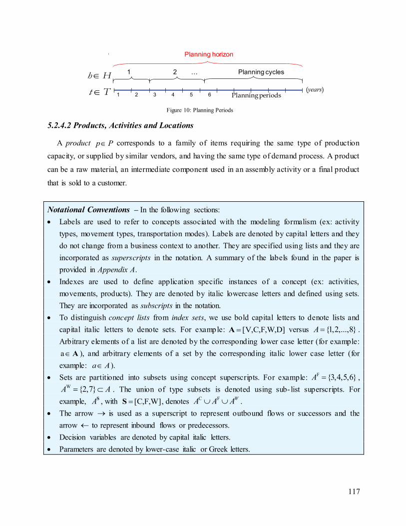
117
5.2.4.2 Products, Activities and Locations
A product p P corresponds to a family of items requiring the same type of production
capacity, or supplied by similar vendors, and having the same type of demand process. A product
can be a raw material, an intermediate component used in an assembly activity or a final product
that is sold to a customer.
Notational Conventions – In the following sections:
Labels are used to refer to concepts associated with the modeling formalism (ex: activity
types, movement types, transportation modes). Labels are denoted by capital letters and they
do not change from a business context to another. They are specified using lists and they are
incorporated as superscripts in the notation. A summary of the labels found in the paper is
provided in Appendix A.
Indexes are used to define application specific instances of a concept (ex: activities,
movements, products). They are denoted by italic lowercase letters and defined using sets.
They are incorporated as subscripts in the notation.
To distinguish concept lists from index sets, we use bold capital letters to denote lists and
capital italic letters to denote sets. For example: [V,C,F,W,D]A versus {1,2,...,8}A .
Arbitrary elements of a list are denoted by the corresponding lower case letter (for example:
aA ), and arbitrary elements of a set by the corresponding italic lower case letter (for
example: a A ).
Sets are partitioned into subsets using concept superscripts. For example: F {3,4,5,6}A ,
W {2,7}A A . The union of type subsets is denoted using sub- list superscripts. For
example, AS, with [C,F,W]S , denotes
C F WA A A .
The arrow is used as a superscript to represent outbound flows or successors and the
arrow to represent inbound flows or predecessors.
Decision variables are denoted by capital italic letters.
Parameters are denoted by lower-case italic or Greek letters.
t T
h H
1 2 3 4 5 6
Planning horizon
1 2 … Planning cycles
Planning periods(years)
Figure 10: Planning Periods
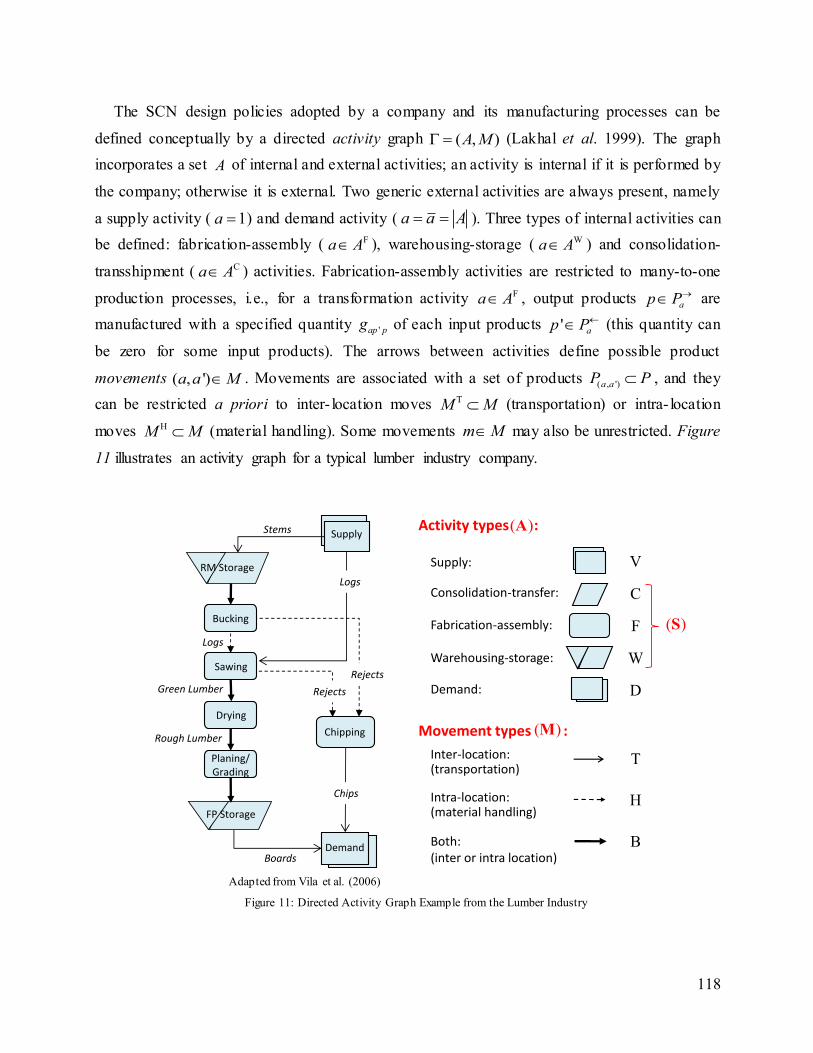
118
The SCN design policies adopted by a company and its manufacturing processes can be
defined conceptually by a directed activity graph ( , )A M (Lakhal et al. 1999). The graph
incorporates a set A of internal and external activities; an activity is internal if it is performed by
the company; otherwise it is external. Two generic external activities are always present, namely
a supply activity ( 1a ) and demand activity ( a a A ). Three types of internal activities can
be defined: fabrication-assembly ( Fa A ), warehousing-storage ( Wa A ) and consolidation-
transshipment ( Ca A ) activities. Fabrication-assembly activities are restricted to many-to-one
production processes, i.e., for a transformation activity Fa A , output products ap P are
manufactured with a specified quantity 'ap pg of each input products ' ap P (this quantity can
be zero for some input products). The arrows between activities define possible product
movements ( , ')a a M . Movements are associated with a set of products ( , ')a aP P , and they
can be restricted a priori to inter- location moves TM M (transportation) or intra- location
moves HM M (material handling). Some movements m M may also be unrestricted. Figure
11 illustrates an activity graph for a typical lumber industry company.
Adapted from Vila et al. (2006)
Figure 11: Directed Activity Graph Example from the Lumber Industry
Supply:
Warehousing-storage:
Demand:
Activity types :
Fabrication-assembly:
Consolidation-transfer:
Movement types :
Inter-location:(transportation)
Intra-location:(material handling)
Both: (inter or intra location)
V
C
F
W
D
T
H
B
( )A
( )M
( )S
Stems Supply
RM Storage
Logs
Rejects
Rejects
Chips
Logs
Boards
Rough Lumber
Green Lumber
Demand
Planing/Grading
FP Storage
Chipping
Bucking
Sawing
Drying
119
The following parameters are defined:
'appg : Quantity of product ap P needed to make one product ' ap P in activity Fa A
paq : Capacity consumption per unit of product ap P flowing through activity a A
pas : Space required per unit of product ap P stored in activity Wa A
Vendors, facility sites and demand zones are associated with geographical locations l L ,
and, accordingly, we distinguish three types of locations: vendor locations (V), site locations (S)
and demand zones (D). Vendor Vl L L can supply products lP P , and demand zone
Dl L L requires products lP P . The demand zones to serve may change from period to
period, and D D
ptL L is the subset of zones requiring product p in period t T . The facility site
locations SL L considered correspond to existing company or third-party facilities, or to
locations where a facility could be operated.
5.2.4.3 Transportation Options
Transportation between locations can be performed using different shipping means s S T,
subdivided according to their transportation mode: air ( AS ), ocean ( OS ), railway ( RS ), driveway
D( )S or intermodal ( IS ), with = A,O,R,D,IT . The network capacity of a shipping mean s S T
during a time period is provided by a set of transportation options o O . These options may be
associated with an internal fleet, a long term 3PL contract or short term for-hire transportation. It
is assumed that a transportation mean is not based at a particular facility site and that it can be
used anywhere in the network provided that the required infrastructures are available. There is a
variable cost associated with the use of a transportation mean and a fixed cost is incurred when an
option is selected. This fixed cost covers fleet terminal, replacement and repair costs, or external
contract costs. Some options may already be in place at the beginning of the planning horizon.
Intra- location moves can be performed using different handling means Hs S with distinct
variable costs. Collectively, transportation and handling means define a set of transfer means
HS S S T.
The following sets, variables and parameters are required to consider transportation options:
shO Capacity options available for shipping mean s S T during planning cycle h.
ohZ : Binary variable equal to 1 if transportation capacity option o O is selected at the
beginning of planning cycle h H .
120
t
pq : Capacity consumption (in handling units) per unit of product p flowing through
reception/shipping facilities for transportation mode tT .
'll s : Traveling time consumed per trip (one way if it is a one-time for-hire mean and
round-trip otherwise) when transportation mean s S T is used on lane ( , ')l l L L .
psu : Transportation capacity consumed (number of vehicle load required) per shipping
unit of product p P when transportation mean s S T is used.
ot : Transportation capacity available (in standard traveling time units) for shipping mean
s(o) in period t when option o O is selected (the capacity provided by some options
may be unbounded).
ot : Minimal usage (in standard traveling time units) of shipping mean s(o) needed in
planning period t to be able to use transportation capacity option o O .
otz : Fixed cost of using transportation capacity option o O during time period t T .
5.2.4.4 Platforms
The facilities already in place are characterized by a platform specifying their capacity for
each of the activities they perform, as well as their fixed and variable costs. Alternative platforms
lc C (facility configurations) can however be considered for each site Sl L . These alternative
platforms may correspond to current layouts, to a reengineering of current layouts or equipments,
to the addition of new space and/or equipment to expand capacity, to different facility
specifications for new sites, or to alternative third-party facilities for a potential location.
Alternative platforms may be associated with different equipment size to capture economies of
scale. For each potential site, a set of possible platforms can thus be considered. For a site Sl L
and planning period t T , a platform lc C is characterized by:
A set of activities C F W
lcA A A A A S supported by the platform.
A capacity, ( , )l a ctb , for each activity lca A , expressed in terms of an upper bound on a
standard capacity measure (production time, storage space…). It is assumed that all the
output products ap P of an activity lca A share the capacity provided by the platform for
this activity. A capacity consumption rate paq is used to convert the throughput of product
ap P in the standard capacity measure.
When platform c is implemented at the beginning of planning cycle h, if ht T , a part
( , ) ( , )l a ct l a ctb of the capacity available for activity a in period t is lost.
121
A minimum throughput, ( , )l a ctb , for each activity lca A , required to implement the platform.
A reception and shipping capacity t
lctb , for each transportation mode t A,O,R,D,I T .
An alternative platform '( )c c which could be used as an upgrade. Upgrade-platform '( )c c
can be implemented only when platform c is in place. Some platforms cannot be upgraded.
A fixed exploitation cost clty for the planning period. This cost includes fixed operating
costs as well as a rent paid for using the platform during period t. When the facility is rented,
or a third-party facility is used, this rent corresponds to the payments made to the facility
owners. When the platform is owned, built, reconfigured or acquired by the company, the n
the rent is the amount that would be obtained if the company was renting the facility on the
market. Normally, this rent would cover financial charges and market value depreciation, and
possibly an opportunity cost, and it would take into account the asset economic life,
associated tax recuperations and the financial horizon of the company.
An implementation cost clty if the platform is installed at the beginning of planning cycle
( )h t . Normally, this cost is positive if the planning period t considered is the first period of
cycle ( )h t , and close to zero otherwise. It is an opening or upgrade project cost paid during
the period and it does not include any capital expenditure. It may include costs related to the
initial provisioning of safety stocks, personnel hiring costs, support activity set-up costs, etc.
A disposal cost (return) clty if the platform is closed at the beginning of planning cycle ( )h t .
This would cover any cash flow incurred in period t following a shutdown in the first period
of cycle ( )h t . It may include costs/returns associated with the repositioning or disposal of
material, equipment and personnel. Closing platform lc C results in the permanent closing
of site l, i.e. when a platform is closed on a site, the site cannot be reopened during the
horizon.
A variable throughput cost ( , )p l a ctx , for each output product ap P of activity lca A ,
covering relevant reception, production, handling and shipping expenses.
The set of activities lA that could be performed on a potential site Sl L depends on the
platforms considered for that site, i.e. ll c C lcA A .
In the model, the following sets, variables and parameters are required:
lhC
Platforms that can be used for site l during cycle h.
( , )l a hC
Platforms that can be used to perform activity a in site l during cycle h.

122
clhY ,clhY ,
clhY : Binary variable equal to 1 if, respectively, opening, using or closing platform
lc C at site Sl L at the beginning of planning cycle h H . 0 , ,cl lY c C are
binary parameters providing the state of site Sl L at the beginning of the horizon.
( , )l a ctb : Maximum capacity available for activity
lca A when platform ( , ) ( )l a h tc C is used
at site Sl L during period t T .
( , )l a chb : Minimum activity level for activity lca A when platform ( , )l a hc C is used at site
Sl L during planning cycle h H .
t
lctb Reception and shipping capacity (in handling units) at site Sl L for transportation
mode tT when platform ( )lh tc C is used during period t T (taking location Sl L transportation infrastructure capabilities into account).
( , )l a ct : Capacity lost for activity a in period t when platform c is implemented at the
beginning of planning cycle h(t).
( , )p l a ctx : Unit cost of processing product p P on platform ( , ) ( )l a h tc C in node ( , )l a
during period t T .
clty ;clty ;
clty : Respectively, unit cost of opening, using and closing platform ( )lh tc C at site
l L S during period t T .
Internal location configurations are specified by the platform selection variables clhY , clhY and
clhY , which must respect the following conditions. Constraint (1) states that no more than a single
platform can be implemented on a site in any given planning cycle. Constraints (2) and (3) ensure
that a site cannot be closed, or opened, more than once during the planning horizon.
1lh
clh
c C
Y
S,l L h H (1)
01olh
clh cl
h H c C
Y Y
Sl L (2)
1lh
clh
h H c C
Y
Sl L (3)
Constraint (4) specifies precedence relations for the upgrade of platforms. An upgrade platform
can only be installed if its preceding platform is already in place and if it is not closed at the
beginning of the cycle. Constraint (5) ensures that platform states are accounted for correctly, i.e.
that a platform can be closed only if it was used during the previous planning cycle, and that a
platform cannot be opened and closed during the same planning cycle.
123
'( ) 1c c lh clh clhY Y Y
S, , lhl L h H c C (4)
'( ) 1 0clh c c lh clh clh clhY Y Y Y Y
S, , lhl L h H c C (5)
5.2.4.5 Vendor Contracts
A vendor may offer different pricing conditions related to guaranteed minimum sales volumes
for each period of a planning cycle. These offers are considered as alternative supply contracts.
To simplify the notation, we consider that alternative contracts offered by a given vendor define
distinct supply sources, and they are all incorporated in the set VL of potential vendors. To model
vendor contracts selection, the following variables and parameters are required:
lhV : Binary variable equal to 1 if vendor contract Vl L is selected for planning cycle h H
.
ltU : Penalty paid to the vendor under contract Vl L if the minimum sales value specified in
the contract is not reached for period t T (decision variable).
pltb : Upper bound on the quantity of product family p P which can be supplied by the
vendor under contract Vl L during period t T .
ltb : Lower bound on the value of products purchased in period t T specified in contract
Vl L .
plt : Unit procurement price of product family p P from vendor Vl L during period t T
.
ltv : Fixed cost of using vendor contract Vl L during period t T .
5.2.4.6 Product-Markets and Marketing Policies
It is assumed that products are sold in a set of distinct product-markets k K . A product-
market k is defined by a geographical region covering a set of demand zones, D D
kL L , in which
a set of product- families, kP P having similar marketing conditions are sold. Three types of
markets can be distinguished: inventory-based replenishment markets (I), made-to-order markets
(O) and vendor managed inventory (VMI) markets (V). The set of product-markets can thus be
partitioned in three subsets k , k =[I,O,V]K K . We assume that a demand zone is associated with
a single market type, i.e. if a geographical location has customers in more than one market type, a
distinct demand zone l is defined for each market type. k(l) denotes the market type of location l,
124
and Dk DL L the set of demand zones in the markets of type k. For a market type kK , a given
product-zone pair ( , )p l thus belongs to a unique product-market k( )( , ) lk p l K . In order to win
orders on these product-markets, the company develops different offers to satisfy potential
customers better than its competitors. It is assumed that these offers must be defined in terms of
delivery response, fill rates and product prices. These offers can be formalized through the
marketing policy concept. We assume that a set kJ of policies is considered for each product-
market k K , and that a policy j is associated with a single product-market ( )k j . A policy
kj J for a product-market kk K is characterized by:
Product prices ( ),jpt k jp p P , when the policy is used in period t.
A maximum delivery time, if the product-market is of the inventory-based replenishment
type, or a minimum fill rate, if it is a VMI product-market. Since it may not be possible to
satisfy the delivery time, or to provide an adequate fill rate, from all the sites in the network,
using any transportation means, because some sites are too far, or some transfer means are
too slow or for any other reason, this leads to the association of a set of admissible (location-
transportation mean) pairs to the policy (defined in the next section as the sets jplNS ).
A fix marketing and logistics cost jtw when the policy is used in period t T . For VMI
product-markets, this cost would include the inventory holding cost incurred at the customer
location to provide the specified fill rate.
A minimum market penetration sales quantity jpltd for product kp P in demand zone
D
kl L
during period t T .
A maximum demand quantity jpltd
for product kp P in demand zone
D
kl L during period
t T .
The following variables and parameters are required to model marketing policies:
jhW : Binary variable equal to 1 if policy j J is selected for product-market ( )k j
during planning cycle h H
jpltd , jpltd : Minimum market penetration quantity and maximum demand quantity for product
family p P in demand zone Dl L when marketing policy j J is selected
during period t T
125
jptp : Unit sales price of product family ( )k jp P during period t T when marketing
policy j J is selected for cycle h(t)
jtw : Fixed cost of using marketing policy j J during period t T
Since market policies represent long-term commitments and strategies rather than sales
planning tactics, a marketing policy is enforced for a planning cycle rather than for a single time
period. The following condition, stating that no more than one market policy can be selected for
each market in each planning cycle, must be respected:
1k
jh
j J
W
,h H k K (6)
When no policy is selected, it implies that the product-market k will not be serviced by the
company during planning cycle h.
5.2.4.7 Supply Chain Network
When the activity graph ( , )A M is mapped onto the potential locations l L , the supply
chain network represented in Figure 12 is obtained. In this network, the nodes correspond to
feasible location-activity pairs ( , )n l a N , and the arcs to feasible product flows between
nodes with a given transfer mean in a given time period t T . In what follows, we use ( )l n and
( )a n to denote, respectively, the location and the activity of node n. A location-activity pair
( , )l a is feasible if la A . A flow between nodes ( , )n l a and ' ( ', ')n l a is not feasible if
T[ '] [( , ') ]l l a a M or if H[ '] [( , ') ]l l a a M . For a given node n, the set of destinations of
feasible outbound arcs is denoted by nN , and the set of origins of feasible inbound arcs by nN .
Note also that, for internal origin-destination pairs ( , ') (( , ),( , '))n n l a l a , parallel arcs exist for
all feasible pairs ( , ') '( , ) a a pnnp s P S , where 'pnnS is the set of transfer means which can be used
for product p between origin n and destination 'n . Similarly, for supply origin-destination pairs
( , ') (( ,1),( ', '))n n l l a , parallel arcs exist for all (1, ) '( , ) ( )a l pnnp s P P S , and for demand origin-
destination pairs ( , ') (( , ),( ', ))n n l a l a , parallel arcs exist for all the products p required by
demand zone l’, and for all transportation means s and policies j which can be implemented from
node n .
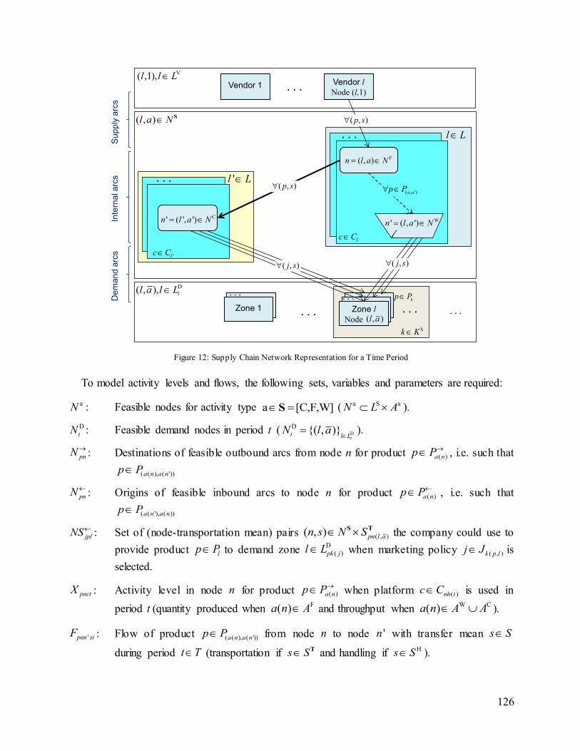
126
Figure 12: Supply Chain Network Representation for a Time Period
To model activity levels and flows, the following sets, variables and parameters are required:
aN : Feasible nodes for activity type a [C,F,W] S ( a S aN L A ).
D
tN : Feasible demand nodes in period t ( D
D {( , )}t
t l LN l a
).
pnN: Destinations of feasible outbound arcs from node n for product ( )a np P , i.e. such that
( ( ), ( '))a n a np P
pnN: Origins of feasible inbound arcs to node n for product ( )a np P , i.e. such that
( ( '), ( ))a n a np P
jplNS: Set of (node-transportation mean) pairs ( , )( , ) pn l an s N S S T
the company could use to
provide product lp P to demand zone D
( )pk jl L when marketing policy ( , )k p lj J is
selected.
pnctX : Activity level in node n for product ( )a np P when platform ( )nh tc C is used in
period t (quantity produced when F( )a n A and throughput when
W C( )a n A A ).
'pnn stF : Flow of product ( ( ), ( '))a n a np P from node n to node 'n with transfer mean s S
during period t T (transportation if s S T and handling if
Hs S ).
l L
F( , )n l a N
lc C
( , ')a ap P
Vendor 1 Vendor l
Node (l,1). . .
. . .
. . .
D( , ), tl a l L
SupplyZone 1 SupplyZone l
Node ( , )l a. . .. . .
( , )l a N S
. . . kp P
( , )p s
kk K
. . .
Su
pp
lya
rcs
Dem
an
da
rcs
Inte
rna
larc
s
V( ,1),l l L
. . . 'l L
'lc C
( , )p s
C' ( ', ')n l a N W' ( , ')n l a N
( , )j s( , )j s
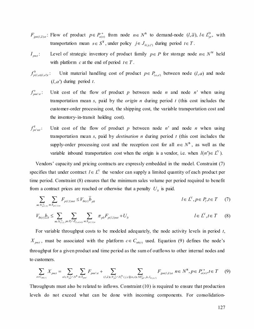
127
( , )jpn l a stF : Flow of product ( )a np P from node n N S to demand-node D( , ), ,ptl a l L with
transportation mean s S T , under policy ( , ')k p lj J during period t T .
pnctI : Level of strategic inventory of product family p P for storage node Wn N held
with platform c at the end of period t T .
( , )( , ')
h
p l a l a tf : Unit material handling cost of product ( , ')a ap P between node ( , )l a and node
( , ')l a during period t.
o
'pnn stf : Unit cost of the flow of product p between node n and node 'n when using
transportation mean s, paid by the origin n during period t (this cost includes the
customer-order processing cost, the shipping cost, the variable transportation cost and
the inventory- in-transit holding cost).
d
'pn nstf : Unit cost of the flow of product p between node 'n and node n when using
transportation mean s, paid by destination n during period t (this cost includes the
supply-order processing cost and the reception cost for all n N S , as well as the
variable inbound transportation cost when the origin is a vendor, i.e. when V( ')l n L ).
Vendors’ capacity and pricing contracts are expressly embedded in the model. Constraint (7)
specifies that under contract Vl L the vendor can supply a limited quantity of each product per
time period. Constraint (8) ensures that the minimum sales volume per period required to benefit
from a contract prices are reached or otherwise that a penalty ltU is paid.
( ,1)( ,1)
( ,1) ( )
p l np l
p l nst lh t plt
s Sn N
F V b
V , ,ll L p P t T (7)
(1, ( )) ( ,1)( ,1)
( ) ( ,1)
l a n p l nl
ltlh t plt p l nst lt
p P P s Sn N
V b F U
V ,l L t T (8)
For variable throughput costs to be modeled adequately, the node activity levels in period t,
pnctX , must be associated with the platform ( )nh tc C
used. Equation (9) defines the node’s
throughput for a given product and time period as the sum of outflows to other internal nodes and
to customers.
D( ) ' ( , )
' ( , )
' ( , ) ( , ) ( , ) ,nh t pnnpn pn t jpl k p l
pnct pnn st jpn l a st
c C s Sn N N l a N N j s n s NS j J
X F F
S
( ), ,a nn N p P t T S (9)
Throughputs must also be related to inflows. Constraint (10) is required to ensure that production
levels do not exceed what can be done with incoming components. For consolidation-
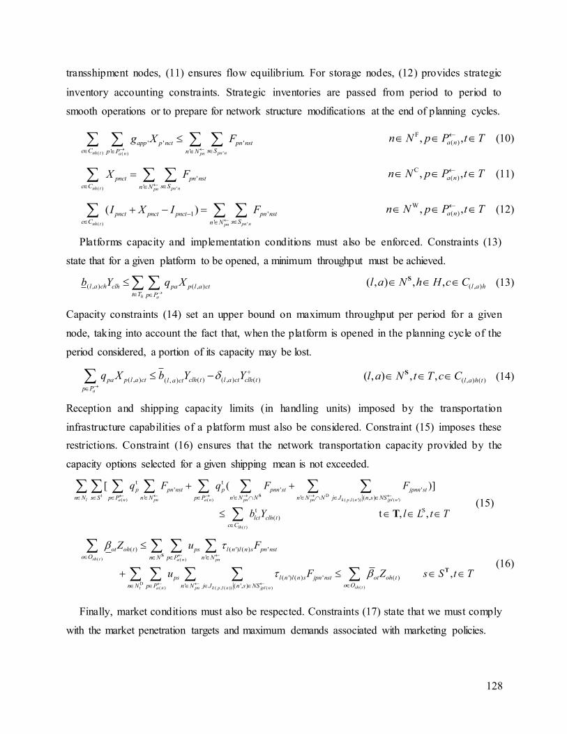
128
transshipment nodes, (11) ensures flow equilibrium. For storage nodes, (12) provides strategic
inventory accounting constraints. Strategic inventories are passed from period to period to
smooth operations or to prepare for network structure modifications at the end of planning cycles.
( ) '( )
' ' '
' 'nh t pn na n pn
app p nct pn nst
c C s Sp P n N
g X F
F
( ), ,a nn N p P t T (10)
( ) '
'
'nh t pn npn
pnct pn nst
c C s Sn N
X F
C
( ), ,a nn N p P t T (11)
( ) '
1 '
'
( )nh t pn npn
pnct pnct pnct pn nst
c C s Sn N
I X I F
W
( ), ,a nn N p P t T (12)
Platforms capacity and implementation conditions must also be enforced. Constraints (13)
state that for a given platform to be opened, a minimum throughput must be achieved.
( , ) ( , )
h a
l a ch clh pa p l a ct
t T p P
b Y q X
( , )( , ) , , l a hl a N h H c C S (13)
Capacity constraints (14) set an upper bound on maximum throughput per period for a given
node, taking into account the fact that, when the platform is opened in the planning cycle of the
period considered, a portion of its capacity may be lost.
( , ) ( ) ( , ) ( )( , )
a
pa p l a ct clh t l a ct clh tl a ct
p P
q X b Y Y
( , ) ( )( , ) , , l a h tl a N t T c C S (14)
Reception and shipping capacity limits (in handling units) imposed by the transportation
infrastructure capabilities of a platform must also be considered. Constraint (15) imposes these
restrictions. Constraint (16) ensures that the network transportation capacity provided by the
capacity options selected for a given shipping mean is not exceeded.
t D( ) ( ) ( , ( ')) ( ')
( )
t t
' ' '
' ' ' ( , )
t
( )
[ ( )]
l a n pn a n pn pn k p l n jpl n
lh t
p pn nst p pnn st jpnn st
n N s S p P n N p P n N N n N N j J n s NS
lct clh t
c C
q F q F F
b Y
S
S t , ,l L t T T (15)
( ) ( )
D( )( ) ( , ( )) ( )
( ) ( ') ( ) '
'
( ') ( ) ' ( )
' ( ', )
,
sh t a n pn
sh tt a n pn k p l n jpl n
ot oh t ps l n l n s pn nst
o O n N p P n N
ps l n l n s jpn nst ot oh t
o On N p P n N j J n s NS
Z u F
u F Z s S t T
S
T (16)
Finally, market conditions must also be respected. Constraints (17) state that we must comply
with the market penetration targets and maximum demands associated with marketing policies.

129
( ) ( , ) ( )
( , ) jpl
jpltjh t jpn l a st jh t jplt
n s NS
W d F W d
D
( , ), , ,t l k p lt T l L p P j J (17)
5.2.4.8 Order Cycle and Safety Stocks
In addition to strategic inventories, order cycle inventories and safety stocks must also be
considered in the model since they depend on storage activity throughputs and on the transfer
means used. The level of these stocks also depends on the operations management policies of the
company and on the ordering behavior of customers. It can be shown (Martel, 2003) that, when
sound inventory management and forecasting methods are used, the relationship between the
throughput pnX of product ( )a np P in storage node W( , )n l a N , the procurement lead time
pn associated with the location of the supply source, the transfer mean used, and the average
cycle and safety stock ( , )pa pn pnI X required to support this throughput takes the form of the
following power function ( , ) ( ) ( )pa pa
pa pn pn pa pn pnI X X
, with , 1pa pa to reflect
economies of scale. The parameters pa , pa and pa of this function are obtained by
regression, from historical or simulation data (Ballou, 1992). We assume here that the throughput
pnX used as an argument in this function is the sum of all product p shipments from node
Wn N to feasible destinations ' nn N .
If the historical throughput level, average lead time and average inventory level observed for a
period (for product p in node n) are o
pnX , o
pn and ( , )o o
pa pn pnI X , respectively, then the ratio
/ ( , )o o o
pn pa pn pnX I X is the familiar inventory turnover ratio, and its inverse
( , ) /o o o o
pn pa pn pn pnI X X is the number of periods of inventory kept in stock. Assuming that the
relationship between inventory level and throughput is linear boils down to approximating
( , )pa pn pnI X by o
pn pnX . Since the facilities’ throughputs, the sourcing location and the transfer
mean are not known before the network design model is solved, and since they can be far from
historical values (mainly if new facilities are opened or existing ones closed), calculating
inventory levels with historical inventory turnover ratios can be completely inadequate. An effort
is therefore made in this paper to take risk pooling effects into account explicitly. Starting from
the inventory-throughput function just defined, and taking into account the average unit inventory
holding cost pnctr of products ( )a np P when platform ( )nh tc C is used at site l(n) during period
t T , the following inventory cycle and safety stock cost function results, when the product is
supplied from node ' pnn N using transfer mean 'pn ns S :
( ) ( )
' ( ) ' ( ) '( , ) ( , ) ( ) ( )pa n pa n
pnct pnct pn ns pnct pa n pnct pn ns pnct pa n pnct pn nsH X r I X r X
(18)
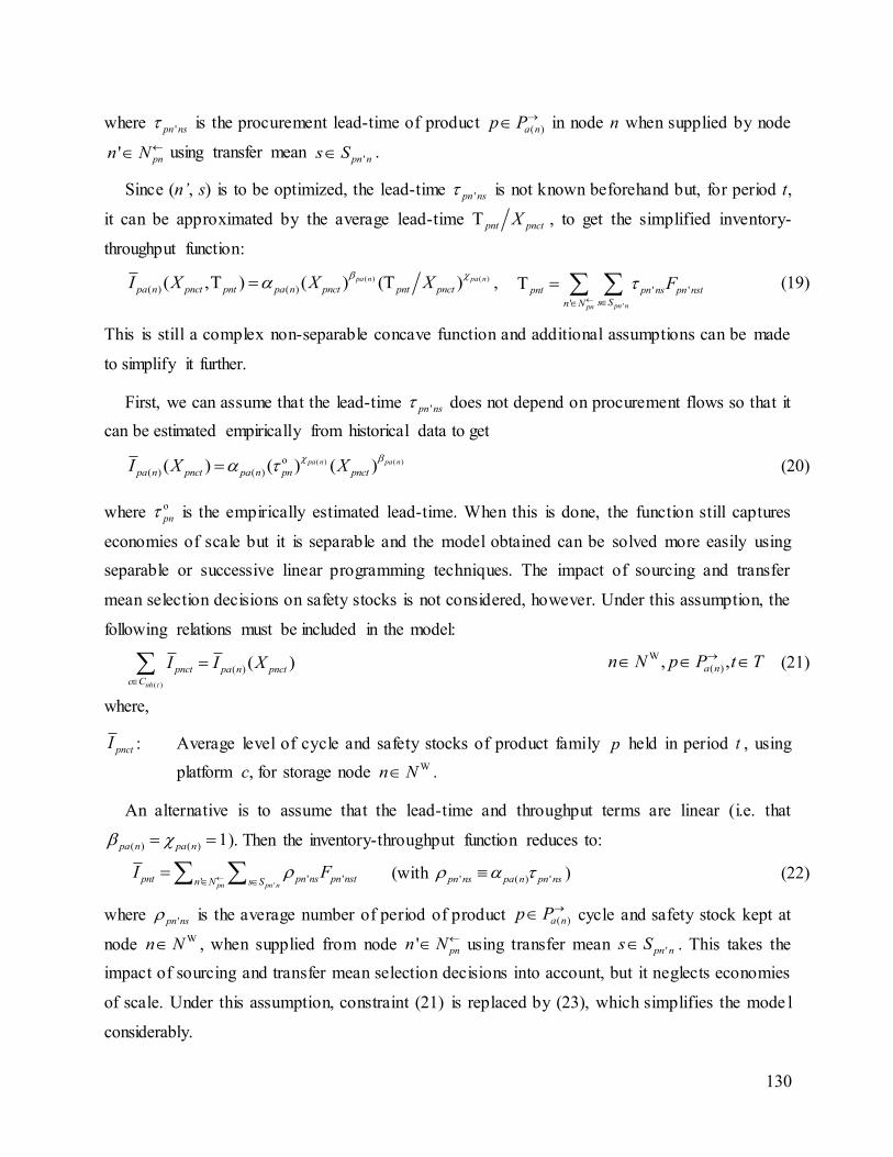
130
where 'pn ns is the procurement lead-time of product ( )a np P in node n when supplied by node
' pnn N using transfer mean 'pn ns S .
Since (n’, s) is to be optimized, the lead-time 'pn ns is not known beforehand but, for period t,
it can be approximated by the average lead-time pnt pnctX , to get the simplified inventory-
throughput function:
( ) ( )
( ) ( )( , ) ( ) ( )pa n pa n
pa n pnct pnt pa n pnct pnt pnctI X X X
,
'
' '
' pn npn
pnt pn ns pn nst
s Sn N
F
(19)
This is still a complex non-separable concave function and additional assumptions can be made
to simplify it further.
First, we can assume that the lead-time 'pn ns does not depend on procurement flows so that it
can be estimated empirically from historical data to get
( ) ( )o
( ) ( )( ) ( ) ( )pa n pa n
pa n pnct pa n pn pnctI X X
(20)
where o
pn is the empirically estimated lead-time. When this is done, the function still captures
economies of scale but it is separable and the model obtained can be solved more easily using
separable or successive linear programming techniques. The impact of sourcing and transfer
mean selection decisions on safety stocks is not considered, however. Under this assumption, the
following relations must be included in the model:
( )
( ) ( )nh t
pnct pa n pnct
c C
I I X
W
( ), ,a nn N p P t T (21)
where,
pnctI : Average level of cycle and safety stocks of product family p held in period t , using
platform c, for storage node Wn N .
An alternative is to assume that the lead-time and throughput terms are linear (i.e. that
( ) ( ) 1pa n pa n ). Then the inventory-throughput function reduces to:
'
' '' pn pn npnt pn ns pn nstn N s S
I F (with ' ( ) 'pn ns pa n pn ns ) (22)
where 'pn ns is the average number of period of product ( )a np P cycle and safety stock kept at
node Wn N , when supplied from node ' pnn N using transfer mean 'pn ns S . This takes the
impact of sourcing and transfer mean selection decisions into account, but it neglects economies
of scale. Under this assumption, constraint (21) is replaced by (23), which simplifies the mode l
considerably.
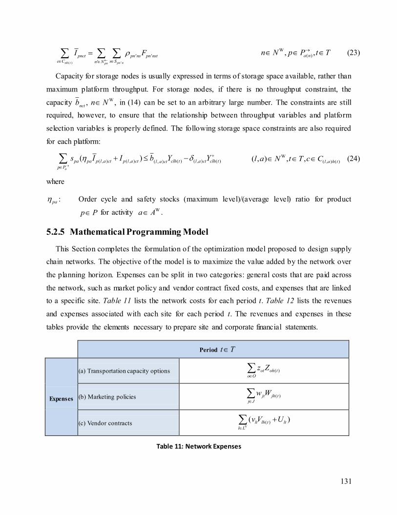
131
( ) '
' '
'nh t pn npn
pnct pn ns pn nst
c C s Sn N
I F
W
( ), ,a nn N p P t T (23)
Capacity for storage nodes is usually expressed in terms of storage space available, rather than
maximum platform throughput. For storage nodes, if there is no throughput constraint, the
capacity W, ,nct
b n N in (14) can be set to an arbitrary large number. The constraints are still
required, however, to ensure that the relationship between throughput variables and platform
selection variables is properly defined. The following storage space constraints are also required
for each platform:
( , ) ( , ) ( ) ( , ) ( )( , )( )
a
pa pa p l a ct p l a ct clh t l a ct clh tl a ct
p P
s I I b Y Y
W
( , ) ( )( , ) , , l a h tl a N t T c C (24)
where
pa : Order cycle and safety stocks (maximum level)/(average level) ratio for product
p P for activity Wa A .
5.2.5 Mathematical Programming Model
This Section completes the formulation of the optimization model proposed to design supply
chain networks. The objective of the model is to maximize the value added by the network over
the planning horizon. Expenses can be split in two categories: general costs that are paid across
the network, such as market policy and vendor contract fixed costs, and expenses that are linked
to a specific site. Table 11 lists the network costs for each period t. Table 12 lists the revenues
and expenses associated with each site for each period t. The revenues and expenses in these
tables provide the elements necessary to prepare site and corporate financial statements.
Table 11: Network Expenses
Period t T
Expenses
(a) Transportation capacity options ( )ot oh t
o O
z Z
(b) Marketing policies ( )jt jh t
j J
w W
(c) Vendor contracts V
( )( )lt lh t lt
l L
v V U
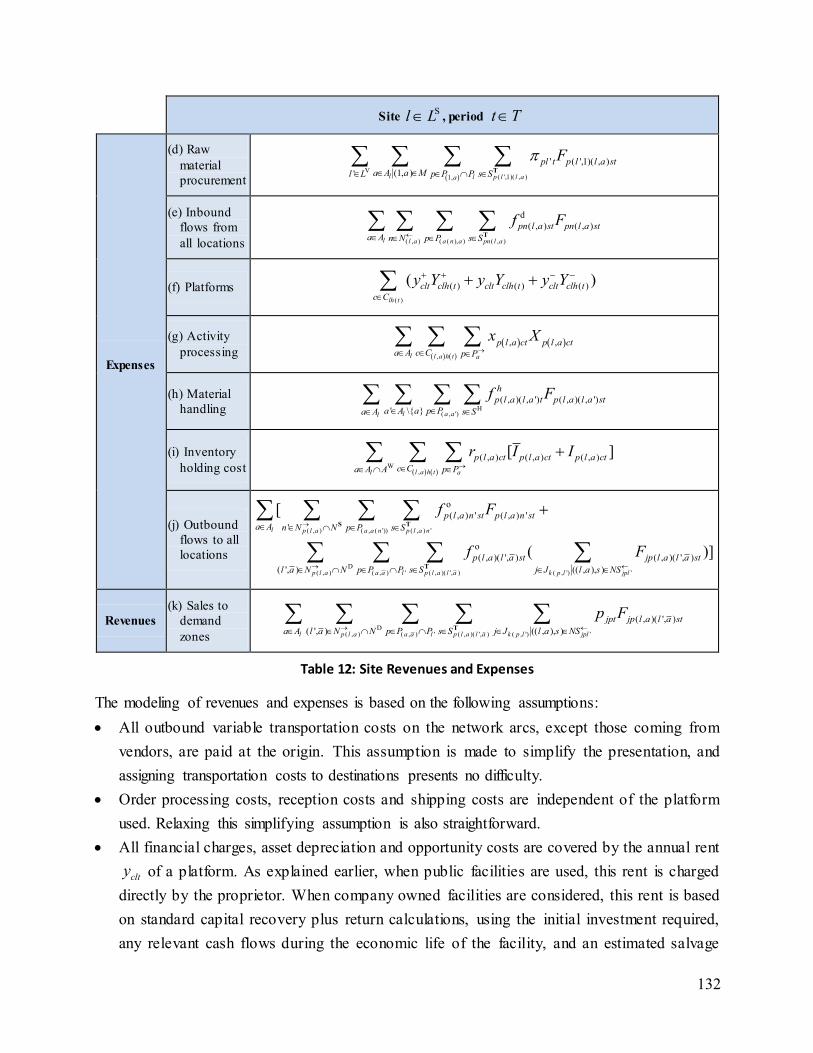
132
Site Sl L , period t T
Expenses
(d) Raw
material
procurement V
( ',1)( , )1,
' ( ',1)( , )
(1, )' l l p l l aa
pl t p l l a st
a A a Ml L p P P s S
F
T
(e) Inbound
flows from
all locations ( , ) ( ( ), ) ( , )
d
( , ) ( , )
l l a a n a pn l a
pn l a st pn l a st
a A n N p P s S
f F
T
(f) Platforms ( )
( ) ( ) ( )( )lh t
clt clh t clt clh t clt clh t
c C
y Y y Y y Y
(g) Activity
processing
,
, ,
l l a h t a
p l a ct p l a cta A c C p P
x X
(h) Material
handling H( , ')
( , )( , ') ( , )( , ')
' \{ }l a al
h
p l a l a t p l a l a st
a A a p Pa A s S
f F
(i) Inventory
holding cost W
,
( , ) ( , ) ( , )[ ]l a h tl a
p l a ct p l a ct p l a ct
c Ca A A p P
r I I
(j) Outbound
flows to all
locations
( , ) ( , ( ')) ( , ) '
D( , ) ( , ) ' ( , )( ', ) ( , ') '
o
( , ) ' ( , ) '
'
o
( , )( ', ) ( , )( ', )
( ', ) (( , ), )
[
( )]
l p l a a a n p l a n
p l a a a l p l a l a k p l jpl
p l a n st p l a n st
a A n N N p P s S
p l a l a st jp l a l a st
l a N N p P P s S j J l a s NS
f F
f F
S T
T
Revenues
(k) Sales to
demand
zones D
( , ) ( , ) ' ( , )( ', ) ( , ') '
( , )( ', )
( ', ) (( , ), )l p l a a a l p l a l a k p l jpl
jpt jp l a l a st
a A l a N N p P P s S j J l a s NS
p F
T
Table 12: Site Revenues and Expenses
The modeling of revenues and expenses is based on the following assumptions:
All outbound variable transportation costs on the network arcs, except those coming from
vendors, are paid at the origin. This assumption is made to simplify the presentation, and
assigning transportation costs to destinations presents no difficulty.
Order processing costs, reception costs and shipping costs are independent of the platform
used. Relaxing this simplifying assumption is also straightforward.
All financial charges, asset depreciation and opportunity costs are covered by the annual rent
clty of a platform. As explained earlier, when public facilities are used, this rent is charged
directly by the proprietor. When company owned facilities are considered, this rent is based
on standard capital recovery plus return calculations, using the initial investment required,
any relevant cash flows during the economic life of the facility, and an estimated salvage
133
value (Peterson, 1969). Relevant cash flows normally include maintenance expenses, property
taxes as well as income tax savings.
Income taxes are taken into account indirectly in the calculations of the facilities rent, as
indicated above. Other than that, it is assumed that tax rates are constant over the planning
horizon and that all taxes are paid under the same jurisdiction. Thus, they do not need to be
included in the model explicitly. When a multinational network is considered, the model is
readily adapted to take country taxes and duties into account, using the guidelines provided in
Vidal and Goetschalckx (2001).
To take all relevant costs into account, financial statements are included for third-party locations
even if they are not controlled by the company.
Let:
Et : Total general network expenditures for period t
Rlt : Total site l revenues for period t
Elt : Total site l expenses for period t
Using the expressions in Tables 1 and 2, revenues and expenditures are calculated as follows:
Et = (a) + (b) + (c) t T (25)
Elt = (d) + (e) + (f) + (g) + (h) + (i) + (j) Sl L , t T (26)
Rlt = (k) Sl L , t T (27)
In our context, the value added by the SCN in period t is given by net operating profits:
S S
( )t lt lt t
l L l L
NOP R E E
t T (28)
The objective of the company is to maximize the sum of discounted net operating profits over the
planning horizon:
(1 )
t
tt T
NOPMax
(29)
where is the weighted average cost of capital of the company.
Based on the previous discussion, the mathematical programming model obtained for the
multi-period activity-based supply chain network design problem considered is the following:
Maximize objective function (29)
134
subject to the following constraints:
- Platform selection constraints (1) – (5)
- Vendor capacity and contract condition constraints (7) and (8)
- Platform throughput calculation and flow equilibrium constraints (9) – (12)
- Platform throughput capacity constraints (13) and (14)
- Reception, shipping and transportation capacity constraints (15) and (16)
- Market policy selection and sales constraints (6) and (17)
- Order cycle and safety stock definition constraints (21) or (23)
- Storage capacity constraints (24)
- Revenue and expenditure definition constraints (25) – (28)
- Non-negativity and binary variable definition constraints:
' 0pnn stF D, \ , ' , ,p P n N N n N s S t T S (30)
' 0jpnn stF D
( , ( ')), , ' , , ,k p l np P n N n N j J s S t T S (31)
0pnctX ( ) ( ), , ,a n nh tn N p P c C t T S (32)
max , 0pnt pntI W
( ), , ,nh tp P n N c C t T (33)
0pnctI W, ,p P n N t T (34)
0ltU V ,l L t T (35)
, , {0,1}clh clh clhY Y Y S, , lhl L h H c C (36)
{0,1}jhW ,j J h H (37)
{0,1}lhV V ,l L h H (38)
{0,1}ohZ o O , h H (39)
5.2.6 Solution Approach
In this Section, we propose an agent-based metaheuristic in order to tackle this SCN design
problem. The algorithm proposed is called CAT (Collaborative Agent Team) and it is based on
the A-Team paradigm. According to Talukdar et al. (2003), “an asynchronous team is a team of
software agents that cooperate to solve a problem by dynamically evolving a shared population of
solutions.” A-Teams have been successfully developed for production planning in the paper
industry (Murthy et al. 1999), for the probe selection problem (Meneses et al. 2008) and for the
resource-constrained project scheduling problem (Ratajczak-Ropel 2010), among others. CAT is
a hybrid distributed solution approach encompassing several types of optimization tec hniques.
The implementation presented here includes mixed- integer linear programs, classical heuristics
and metaheuristics.
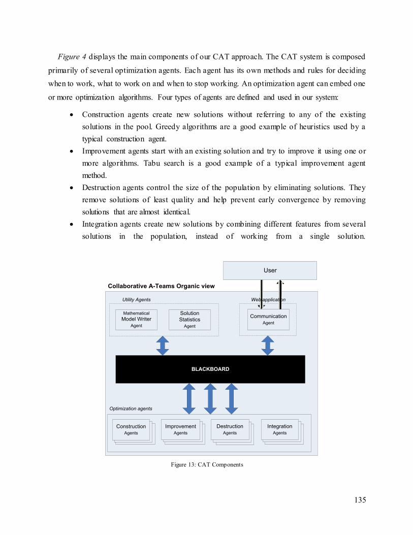
135
Figure 4 displays the main components of our CAT approach. The CAT system is composed
primarily of several optimization agents. Each agent has its own methods and rules for deciding
when to work, what to work on and when to stop working. An optimization agent can embed one
or more optimization algorithms. Four types of agents are defined and used in our system:
Construction agents create new solutions without referring to any of the existing
solutions in the pool. Greedy algorithms are a good example of heuristics used by a
typical construction agent.
Improvement agents start with an existing solution and try to improve it using one or
more algorithms. Tabu search is a good example of a typical improvement agent
method.
Destruction agents control the size of the population by eliminating solutions. They
remove solutions of least quality and help prevent early convergence by removing
solutions that are almost identical.
Integration agents create new solutions by combining different features from several
solutions in the population, instead of working from a single solution.
Figure 13: CAT Components
Collaborative A-Teams Organic view
BLACKBOARD
Optimization agents
Construction
Agents
Destruction
Agents
Utility Agents
Integration
Agents
Communication
Agent
User
Web application
Mathematical
Model Writer
Agent
Solution
Statistics
Agent
Improvement
Agents
136
The blackboard acts as a memory and a hub for all communications. It consists of two
components: the population of solutions and a repository of statistics. As shown in Figure 4
agents communicate solely through the blackboard interface and do not exchange information
directly. New solutions, or partial solutions, are put on the blackboard and existing solutions are
retrieved when necessary. Support agents are also provided to assist the user or the other agents.
The user interacts with CAT through a web application agent.
One of the main advantages of a distributed approach such as CAT is that each agent may
have its own representation of the problem to be solved. For example, one agent may focus on
location decisions while another optimizes annual product flows over the entire supply chain
network. This allows us to decompose the supply chain network design problem over three
dimensions:
The functional dimension refers to the interrelations between different supply chain
decisions such as purchasing and vendor selection decisions, production-distribution
facility location and platform selection decisions, marketing policy choices, and
transportation capacity options selection.
The spatial dimension refers to the geographical positioning of business entities such as
sales territories, national divisions or subsidiaries.
The temporal dimension refers to the nature of the multi-period problem. One could focus
on periodic decisions related to flows, throughputs and inventories, or on strategic options
that span over a specific planning cycle.
Each agent can have either an integrated or decomposed view of each dimension. As a result,
most agents work on different subproblems instead of working on the complete formulation. The
CAT implementation presented here hosts 16 different agents.
Table 13 presents the most important features of each agent; its name, its type, the number of
different heuristics it implements, as well as whether the agent has an integrated (full) or
decomposed (partial) view over each of the problem dimensions. Since CAT uses 40 different
heuristics, it is not possible to provide the pseudo-code for each algorithm. Instead, a general
outlook of the approach used by each agent is provided, along with references to similar
heuristics. All heuristics and agents are coded in C# and VB.NET 2005, and each agent is an
executable program.
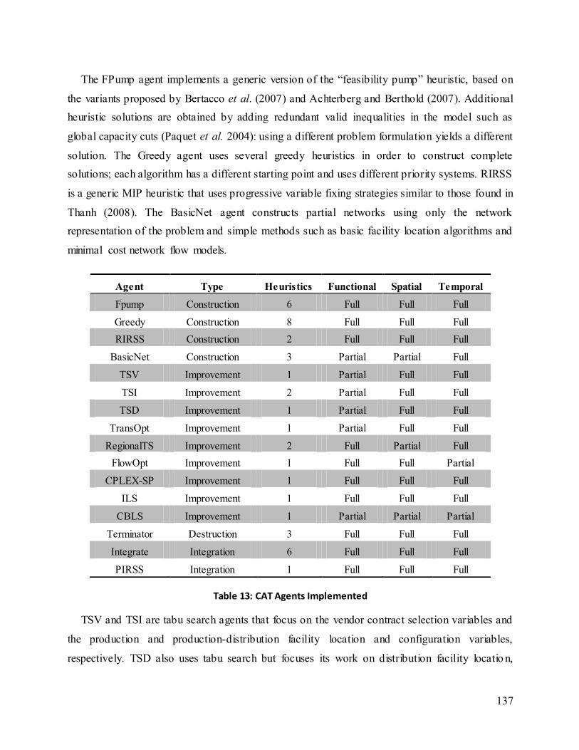
137
The FPump agent implements a generic version of the “feasibility pump” heuristic, based on
the variants proposed by Bertacco et al. (2007) and Achterberg and Berthold (2007). Additional
heuristic solutions are obtained by adding redundant valid inequalities in the model such as
global capacity cuts (Paquet et al. 2004): using a different problem formulation yields a different
solution. The Greedy agent uses several greedy heuristics in order to construct complete
solutions; each algorithm has a different starting point and uses different priority systems. RIRSS
is a generic MIP heuristic that uses progressive variable fixing strategies similar to those found in
Thanh (2008). The BasicNet agent constructs partial networks using only the network
representation of the problem and simple methods such as basic facility location algorithms and
minimal cost network flow models.
Table 13: CAT Agents Implemented
TSV and TSI are tabu search agents that focus on the vendor contract selection variables and
the production and production-distribution facility location and configuration variables,
respectively. TSD also uses tabu search but focuses its work on distribution facility locatio n,
Agent Type Heuristics Functional Spatial Temporal
Fpump Construction 6 Full Full Full
Greedy Construction 8 Full Full Full
RIRSS Construction 2 Full Full Full
BasicNet Construction 3 Partial Partial Full
TSV Improvement 1 Partial Full Full
TSI Improvement 2 Partial Full Full
TSD Improvement 1 Partial Full Full
TransOpt Improvement 1 Partial Full Full
RegionalTS Improvement 2 Full Partial Full
FlowOpt Improvement 1 Full Full Partial
CPLEX-SP Improvement 1 Full Full Full
ILS Improvement 1 Full Full Full
CBLS Improvement 1 Partial Partial Partial
Terminator Destruction 3 Full Full Full
Integrate Integration 6 Full Full Full
PIRSS Integration 1 Full Full Full
138
configuration and marketing policy selection variables. RegionalTS is also a tabu search which
operates on all decision variables relevant to a small portion of the territory covered by the
company’s supply chain network; this portion usually refers to one of the sales territories or a
zone dynamically constructed by the agent itself. TransOpt uses a similar mechanism to optimize
transportation options selection and transportation mean usage across the whole network. All
tabu search algorithms have a similar structure to the tabu search found in Sörensen (2002) and
the variable neighbourhood search heuristic of Amrani et al. (2011). FlowOpt solves a network
flow problem over the supply chain network; the heuristic fixes the value of all binary variables
and then runs the resulting pure linear programming model with the CPLEX® solver. CPLEX-SP
uses the same mathematical formulation as the FPump agent but implements the solution
polishing feature available in CPLEX® 12.1. ILS is an iterated local search type heuristic whose
implementation is similar to the ILS found in Cordeau et al. (2008).
CBLS is a local search heuristic whose main objective is to explore new solution spaces rather
than finding near-optimal solutions to the optimization problem. As such, it constructs a special
tabu list which is composed of the variables that have the same value across most of all solutions
in the population. Although the solutions it yields are not of exceptional quality, it is very
effective for diversification purposes. This agent starts whenever two phenomena are observed
simultaneously: solution quality ceases to improve within the solution pool and solution diversity
decreases.
The Integrate agent combines features from different solutions into a single solution. For
example, vendor selection options from a solution can be integrated with facility configurations
and marketing policy selections from another solution. Improvements are then made until a
strong local optimum is reached. This agent also uses solution combination heuristics inspired
from the crossover operators found in genetic algorithms. PIRSS is an agent that uses a scatter-
search type algorithm; it effectively models the solution space formed by the union of two
complete solutions as a restricted MIP then explores it thoroughly using CPLEX®.
5.2.7 Computational Results
In order to validate and assess our solution approach, a set of 15 benchmark problem instances
were generated. These instances are based on the supply chain network structure of the Usemore
case presented originally in Ballou (1992) and extended in Amrani et al. (2011). The case
represents a typical B2B company manufacturing and selling products through the United States.
139
Product demands and prices, transportation costs as well as the fixed and va riable costs of each
platform, vendor offer and transportation options are randomly generated but are based on
realistic parameter value ranges found in Ballou (1992).
The potential supply chain network comprises 6 to 12 potential production-distribution
facilities, 40 to 48 potential distribution centers, 192 demand zones representing clusters of
customers in the vicinity of major U.S. cities, and 50 to 300 vendor offers. For the production-
distribution facilities, 8 alternative base platforms are considered, and up to 4 potential upgrades
are available per base platform. For the distribution facilities, 5 alternative base platforms are
considered, with a maximum of 2 upgrades per base platforms. The upgrades are mutually
exclusive. Up to 5 product families are sold to the customers while 10 products are used
primarily as components. Various transport capacity options are modeled; TL and LTL shipping
is considered, both in the form of a limited-size private fleet, long-term truck leasing as well as
the use of a common carrier. Five marketing policies are defined for each product.
Of the 15 benchmark instances, 5 are modeled with linear inventory-throughput relationships
using equation (23); they are labeled as PL-01 to PL-05. The remaining instances (PC-06 to PC-
15) have concave inventory-throughput functions (using equation (21)). For those instances,
when the model is solved with the CPLEX solver, the concave functions are approximated by 3-
segments piecewise linear functions using the procedure described in Amrani et al. (2011). For
each of the benchmark instances, the performance of our heuristic is compared to the best
solution found by IBM’s ILOG CPLEX 12.1 solver. All default CPLEX parameters were used.
Experiments were performed on a dual 2.0 GHz 64-bit Intel Xeon® QuadCore computer with 16
GB of RAM. Both CPLEX and CAT were allowed to use the eight processor cores as needed.
Since the benchmarks presented here are very challenging problems, neither our heuristic nor
CPLEX 12.1 reaches a provable global optimum in a reasonable amount of time. We thus present
two sets of results obtained respectively with 1-hour and 8-hour computational time limits.
Interestingly, CPLEX 12.1’s performance varies considerably from run to run while executing in
the parallel mode. When enforcing a fixed time limit, variations on the solution value obtained by
CPLEX are thus observed. Each solution method was run 10 times and both the average of all
runs and the value of the best run are listed.
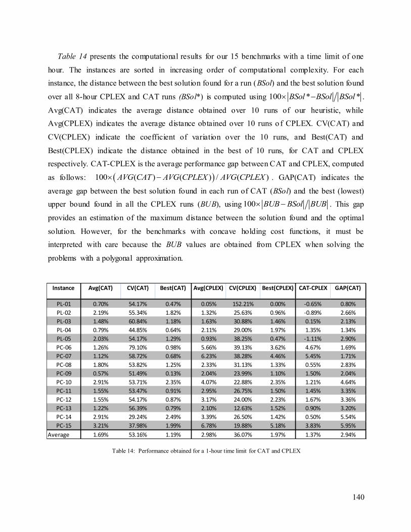
140
Table 14 presents the computational results for our 15 benchmarks with a time limit of one
hour. The instances are sorted in increasing order of computational complexity. For each
instance, the distance between the best solution found for a run (BSol) and the best solution found
over all 8-hour CPLEX and CAT runs (BSol*) is computed using 100 * *BSol BSol BSol .
Avg(CAT) indicates the average distance obtained over 10 runs of our heuristic, while
Avg(CPLEX) indicates the average distance obtained over 10 runs o f CPLEX. CV(CAT) and
CV(CPLEX) indicate the coefficient of variation over the 10 runs, and Best(CAT) and
Best(CPLEX) indicate the distance obtained in the best of 10 runs, for CAT and CPLEX
respectively. CAT-CPLEX is the average performance gap between CAT and CPLEX, computed
as follows: 100 ( ) ( ) / ( )AVG CAT AVG CPLEX AVG CPLEX . GAP(CAT) indicates the
average gap between the best solution found in each run of CAT (BSol) and the best (lowest)
upper bound found in all the CPLEX runs (BUB), using 100 BUB BSol BUB . This gap
provides an estimation of the maximum distance between the solution found and the optimal
solution. However, for the benchmarks with concave holding cost functions, it must be
interpreted with care because the BUB values are obtained from CPLEX when solving the
problems with a polygonal approximation.
Instance Avg(CAT) CV(CAT) Best(CAT) Avg(CPLEX) CV(CPLEX) Best(CPLEX) CAT-CPLEX GAP(CAT)
PL-01 0.70% 54.17% 0.47% 0.05% 152.21% 0.00% -0.65% 0.80%
PL-02 2.19% 55.34% 1.82% 1.32% 25.63% 0.96% -0.89% 2.66%
PL-03 1.48% 60.84% 1.18% 1.63% 30.88% 1.46% 0.15% 2.13%
PL-04 0.79% 44.85% 0.64% 2.11% 29.00% 1.97% 1.35% 1.34%
PL-05 2.03% 54.17% 1.29% 0.93% 38.25% 0.47% -1.11% 2.90%
PC-06 1.26% 79.10% 0.98% 5.66% 39.13% 3.62% 4.67% 1.69%
PC-07 1.12% 58.72% 0.68% 6.23% 38.28% 4.46% 5.45% 1.71%
PC-08 1.80% 53.82% 1.25% 2.33% 31.13% 1.33% 0.55% 2.83%
PC-09 0.57% 51.49% 0.13% 2.04% 23.99% 1.10% 1.50% 2.04%
PC-10 2.91% 53.71% 2.35% 4.07% 22.88% 2.35% 1.21% 4.64%
PC-11 1.55% 53.47% 0.91% 2.95% 26.75% 1.50% 1.45% 3.35%
PC-12 1.55% 54.17% 0.87% 3.17% 24.00% 2.23% 1.67% 3.36%
PC-13 1.22% 56.39% 0.79% 2.10% 12.63% 1.52% 0.90% 3.20%
PC-14 2.91% 29.24% 2.49% 3.39% 26.50% 1.42% 0.50% 5.54%
PC-15 3.21% 37.98% 1.99% 6.78% 19.88% 5.18% 3.83% 5.95%
Average 1.69% 53.16% 1.19% 2.98% 36.07% 1.97% 1.37% 2.94%
Table 14: Performance obtained for a 1-hour time limit for CAT and CPLEX
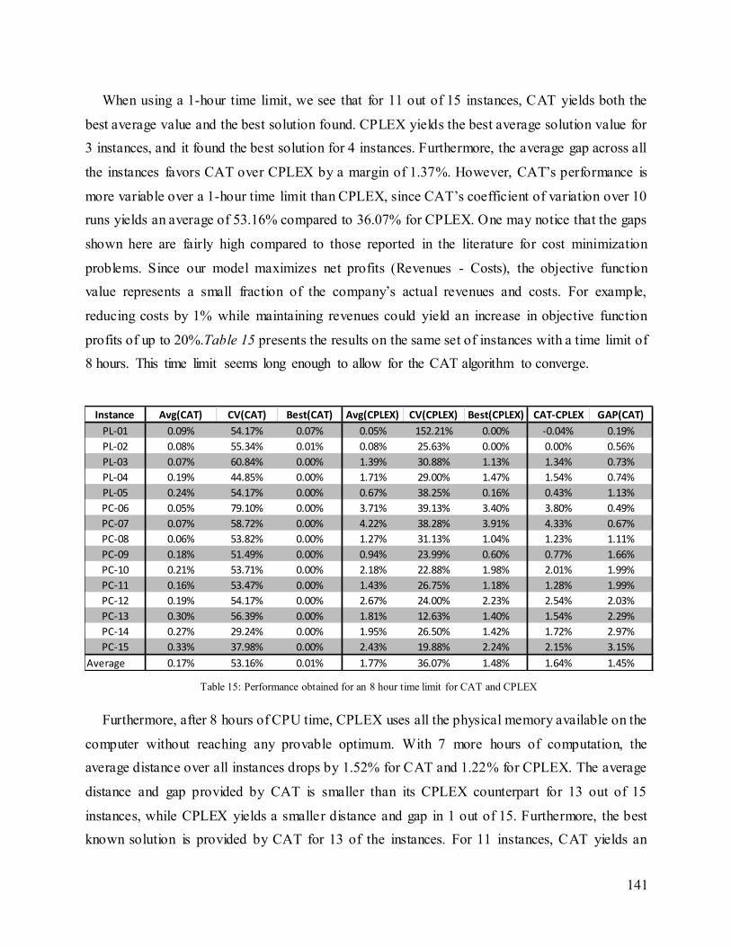
141
When using a 1-hour time limit, we see that for 11 out of 15 instances, CAT yields both the
best average value and the best solution found. CPLEX yields the best average solution value for
3 instances, and it found the best solution for 4 instances. Furthermore, the average gap across all
the instances favors CAT over CPLEX by a margin of 1.37%. However, CAT’s performance is
more variable over a 1-hour time limit than CPLEX, since CAT’s coefficient of variation over 10
runs yields an average of 53.16% compared to 36.07% for CPLEX. One may notice that the gaps
shown here are fairly high compared to those reported in the literature for cost minimization
problems. Since our model maximizes net profits (Revenues - Costs), the objective function
value represents a small fraction of the company’s actual revenues and costs. For example,
reducing costs by 1% while maintaining revenues could yield an increase in objective function
profits of up to 20%.Table 15 presents the results on the same set of instances with a time limit of
8 hours. This time limit seems long enough to allow for the CAT algorithm to converge.
Furthermore, after 8 hours of CPU time, CPLEX uses all the physical memory available on the
computer without reaching any provable optimum. With 7 more hours of computation, the
average distance over all instances drops by 1.52% for CAT and 1.22% for CPLEX. The average
distance and gap provided by CAT is smaller than its CPLEX counterpart for 13 out of 15
instances, while CPLEX yields a smaller distance and gap in 1 out of 15. Furthermore, the best
known solution is provided by CAT for 13 of the instances. For 11 instances, CAT yields an
Instance Avg(CAT) CV(CAT) Best(CAT) Avg(CPLEX) CV(CPLEX) Best(CPLEX) CAT-CPLEX GAP(CAT)
PL-01 0.09% 54.17% 0.07% 0.05% 152.21% 0.00% -0.04% 0.19%
PL-02 0.08% 55.34% 0.01% 0.08% 25.63% 0.00% 0.00% 0.56%
PL-03 0.07% 60.84% 0.00% 1.39% 30.88% 1.13% 1.34% 0.73%
PL-04 0.19% 44.85% 0.00% 1.71% 29.00% 1.47% 1.54% 0.74%
PL-05 0.24% 54.17% 0.00% 0.67% 38.25% 0.16% 0.43% 1.13%
PC-06 0.05% 79.10% 0.00% 3.71% 39.13% 3.40% 3.80% 0.49%
PC-07 0.07% 58.72% 0.00% 4.22% 38.28% 3.91% 4.33% 0.67%
PC-08 0.06% 53.82% 0.00% 1.27% 31.13% 1.04% 1.23% 1.11%
PC-09 0.18% 51.49% 0.00% 0.94% 23.99% 0.60% 0.77% 1.66%
PC-10 0.21% 53.71% 0.00% 2.18% 22.88% 1.98% 2.01% 1.99%
PC-11 0.16% 53.47% 0.00% 1.43% 26.75% 1.18% 1.28% 1.99%
PC-12 0.19% 54.17% 0.00% 2.67% 24.00% 2.23% 2.54% 2.03%
PC-13 0.30% 56.39% 0.00% 1.81% 12.63% 1.40% 1.54% 2.29%
PC-14 0.27% 29.24% 0.00% 1.95% 26.50% 1.42% 1.72% 2.97%
PC-15 0.33% 37.98% 0.00% 2.43% 19.88% 2.24% 2.15% 3.15%
Average 0.17% 53.16% 0.01% 1.77% 36.07% 1.48% 1.64% 1.45%
Table 15: Performance obtained for an 8 hour time limit for CAT and CPLEX
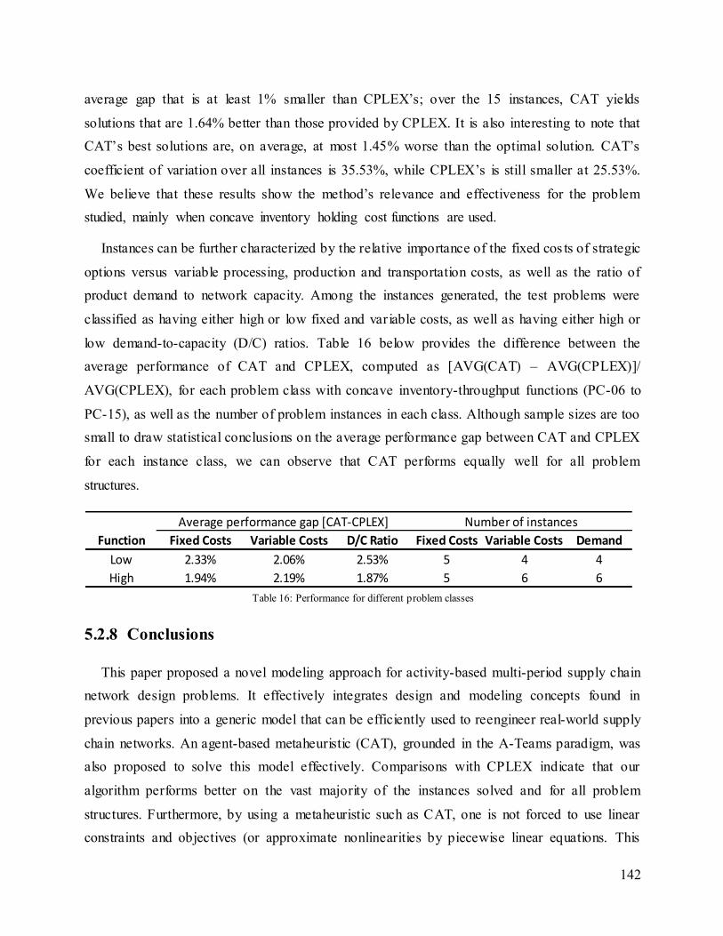
142
average gap that is at least 1% smaller than CPLEX’s; over the 15 instances, CAT yields
solutions that are 1.64% better than those provided by CPLEX. It is also interesting to note that
CAT’s best solutions are, on average, at most 1.45% worse than the optimal solution. CAT’s
coefficient of variation over all instances is 35.53%, while CPLEX’s is still smaller at 25.53%.
We believe that these results show the method’s relevance and effectiveness for the problem
studied, mainly when concave inventory holding cost functions are used.
Instances can be further characterized by the relative importance of the fixed cos ts of strategic
options versus variable processing, production and transportation costs, as well as the ratio of
product demand to network capacity. Among the instances generated, the test problems were
classified as having either high or low fixed and variable costs, as well as having either high or
low demand-to-capacity (D/C) ratios. Table 16 below provides the difference between the
average performance of CAT and CPLEX, computed as [AVG(CAT) – AVG(CPLEX)]/
AVG(CPLEX), for each problem class with concave inventory-throughput functions (PC-06 to
PC-15), as well as the number of problem instances in each class. Although sample sizes are too
small to draw statistical conclusions on the average performance gap between CAT and CPLEX
for each instance class, we can observe that CAT performs equally well for all problem
structures.
5.2.8 Conclusions
This paper proposed a novel modeling approach for activity-based multi-period supply chain
network design problems. It effectively integrates design and modeling concepts found in
previous papers into a generic model that can be efficiently used to reengineer real-world supply
chain networks. An agent-based metaheuristic (CAT), grounded in the A-Teams paradigm, was
also proposed to solve this model effectively. Comparisons with CPLEX indicate that our
algorithm performs better on the vast majority of the instances solved and for all problem
structures. Furthermore, by using a metaheuristic such as CAT, one is not forced to use linear
constraints and objectives (or approximate nonlinearities by piecewise linear equations. This
Function Fixed Costs Variable Costs D/C Ratio Fixed Costs Variable Costs Demand
Low 2.33% 2.06% 2.53% 5 4 4
High 1.94% 2.19% 1.87% 5 6 6
Average performance gap [CAT-CPLEX] Number of instances
Table 16: Performance for different problem classes
143
opens up new modeling opportunities. Furthermore, the CAT metaheuristic can easily be
extended and improved by adding new agents as needed.
There are two main avenues to extend this work. From a CAT implementation perspective,
much could be done to increase the efficiency of agents and reduce the time spent on
nonproductive tasks such as writing and reading solutions. From the SCN modeling point of
view, the model presented could be extended to incorporate financial constraints, international
factors and reverse logistics structures. Finally, in order to account for the uncertainty inherent in
these multi-period problems, a scenario-based stochastic programming version of the model
could and should be elaborated.
5.2.9 References
[52] Achterberg, T., Berthold, T.; Improving the Feasibility Pump, Discrete Optimization, 4, 77-86,
2007.
[53] Altiparmak F., Gen M., Lin L., Paksoy T.; A genetic algorithm approach for multi-objective
optimization of supply chain networks, Computers & Industrial Engineering, 51, 197-216, 2006.
[54] Altiparmak F., Gen M., Lin L., Karaoglan I.; A steady-state genetic algorithm for multi-product
supply chain network design, Computers & Industrial Engineering, 56, 521-537, 2009.
[55] Amiri A.; Designing a distribution network in a supply chain system: Formulation and efficient
solution procedure, European Journal of Operational Research, 171, 567-576, 2006.
[56] Amrani H., Martel A., Zufferey N., Makeeva P.; A variable neighborhood search heuristic for the
design of multicommodity production-distribution networks with alternative facility configuration,
OR Spectrum, 33(4), 989-1007, 2011.
[57] Arntzen B., Brown G., Harrisson T., Trafton L., Global supply chain management at Digital
Equipment Corporation, Interfaces, 21(1), 69-93, 1995.
[58] Bachlaus M., et al.; Designing an integrated multi-echelon agile supply chain network: a hybrid
taguchi-particle swarm optimization approach, Journal of Intelligent Manufacturing, 19(6), 747-
761, 2008.
[59] Balinski M., Fixed-cost Transportation Problems, Naval Research Logistics Quarterly, 8: 41-54,
1961.
144
[60] Ballou R.H., Business Logistics Management, 3rd ed., Prentice Hall, 1992.
[61] Bertacco, L., Fischetti, M., Lodi, A.; A feasibility pump heuristic for general mixed-integer
problems, Discrete Optimization, 4, 63-76, 2007.
[62] Camm J.D., et al.; Blending OR/MS, Judgement, and GIS: Restructuring P&G’s supply chain,
Interfaces, 27(1), 128-142, 1997.
[63] Chaabane A., Ramudhin A., Paquet M.; Design of sustainable supply chains under the emission
trading scheme, International Journal of Production Economics, 135, 37-49, 2012.
[64] Chouinard M., D’Amours S., Aït-Kadi D.; A stochastic programming approach for designing
supply loops, International Journal of Production Economics, 113, 657-677, 2008.
[65] Cooke J., Weaving 2 supply chains together, CSCMP’s Supply Chain Quarterly, 3, 34-38, 2007.
[66] Cordeau, J.-F., Laporte, G., Pasin, F.; An Iterated Local Search Heuristic for the Logistics Network
Design Problem with Single Assignment, International Journal of Production Economics, 113,
626-640, 2008.
[67] Cordeau J.F., Pasin F., Solomon M.M.; An integrated model for logistics network design, Annals of
Operations Research, 144(1), 59-82, 2006.
[68] Denton B.T., Forrest J., Milne R.J.; IBM Solves a Mixed-Integer Program to Optimize Its
Semiconductor Supply Chain, Interfaces, 36(5), 386-399, 2006.
[69] Dogan K., Goetschalckx M., A primal decomposition method for the integrated design of multi-
period production-distribution systems, IIE Transactions, 31, 1027-1036, 1999.
[70] Easwaran G., Üster H.; A closed-loop supply chain network design problem with integrated forward
and reverse channel decisions, IIE Transactions, 42, 779-792, 2010.
[71] Elhedhli S., Goffin J.L.; Efficient Production-Distribution System Design, Management Science,
51:7, 1151-1164, 2005.
[72] Eppen G.D., Martin R.K., Schrage L.; A scenario approach to capacity planning, Operations
Research, 37:4, 517-527, 1989.
[73] Fleischmann B., Ferber S., Henrich P.; Strategic Planning of BMW’s Global Production Network,
Interfaces, 36(3), 194-208, 2006.
145
[74] Geoffrion A., Graves G., Multicommodity Distribution System Design by Benders Decomposition,
Management Science, 20, 822-844, 1974.
[75] Geoffrion A., Powers R., Twenty years of strategic distributon system design: Evolutionary
perspective, Interfaces, 25(5), 105-127, 1995.
[76] Goetschalckx M., Vidal C.J., Dogan K.; Modeling and design of global logistics systems: A review
of integrated strategic and tactical models and design algorithms, European Journal of Operational
Research, 143, 1-18, 2002.
[77] Hansen P., Brimberg J., Urosevic D., Mladenovic N.; Primal-Dual Variable Neighborhood Search
for the Simple Plant-Location Problem, INFORMS Journal on Computing, 19(4), 552-564, 2007.
[78] Ilgin M.A., Gupta S.M.; Environmentally conscious manufacturing and product recovery
(ECMPRO): A review of the state of the art, Journal of Environmental Management, 91, 563-591,
2010.
[79] Jayaraman V., Ross A.; A simulated annealing methodology to distribution network design and
management, European Journal of Operational Research, 144, 629-645, 2003.
[80] Klibi W., Martel A., Guitouni A.; The design of robust value-creating supply chain networks: A
critical review. European Journal of Operational Research, 203, 283-293, 2010.
[81] Klose A.; A Lagrangean relax-and-cut approach for two-stage capacitated facility location problem,
European Journal of Operational Research, 126: 408-421, 2000.
[82] Klose A., Drexl A.; Facility location models for distribution system design, European Journal of
Operational Research, 162: 4-29, 2005.
[83] Lakhal S., Martel A, Oral M, Montreuil B.; Network companies and competitiveness: A framework
for analysis, European Journal of Operational Research, 118, 278-294, 1999.
[84] Liang D., Wilhelm W.E.; Decomposition schemes and acceleration techniques in application to
production-assembly-distribution system design, Computers & Operations Research, 35, 4010-
4026, 2008.
[85] Lin L., Gen M., Wang X.; Integrated multistage logistics network design by using hybrid
evolutionary algorithm, Computers and Industrial Engineering, 56, 854-873, 2009.
146
[86] Martel A.; Généralisations du modèle d’optimisation d’un réseau de ravitaillement. Document de
formation DF-2.4.2, CIRRELT, Université Laval, Canada, 2003.
[87] Martel A.; The Desing of Production-Distribution Networks : A Mathematical Programming
Approach, Springer, in J. Geunes and P.M. Pardalos (eds), Supply Chain Optimization, 265-306,
2005.
[88] Martel A., Benmoussa A., Carle M-A. and Girard S.; A Multi-Period Activity Based Supply Chain
Network Design Model, Technical Report, DRESNET Project, FSA, Université Laval, 2010.
[89] M’Barek, Wissem, Alain Martel and Sophie D’Amours, Designing Multinational Value-Creating
Supply Chain Networks for the Process Industry, Research Paper CIRRELT-2010-51, CIRRELT,
Université Laval, 2010.
[90] Meixell M.J. and Gargeya V.B., Global Supply Chain Design: A Literature Review and Critique,
Transportation Research, Part E, 41, pp.531-550, 2005.
[91] Meneses, C.N., Pardalos, P.M., Ragle M.; Asynchronous Teams for probe selection problems,
Discrete Optimization, 5, 74-87, 2008.
[92] Murthy, S., R. Akkiraju, R. Goodwin, P. Keskinocak, J. Rachlin, F. Wu, J. Yeh, R. Fuhrer, S.
Kumaran, Al. Aggarwal, M. Sturzenbecker, R. Jayaraman and R. Daigle; Cooperative
Multiobjective Decision Support for the Paper Industry, Interfaces, 29(5), 5-30, 1999.
[93] Pan S., Ballot E., Fontane F.; The reduction of greenhouse gas emissions from freight transport by
pooling supply chains, International Journal of Production Economics, In Press,
doi:10.1016/j.ijpe.2010.10.023, 2010.
[94] Paquet M., Martel A., Desaulniers G.; Including Technology Selection Decisions in Manufacturing
Network Design Models, International Journal of Computer Integrated Manufacturing , 17: 117-
125, 2004.
[95] Paquet M., Martel A., Montreuil B.; A manufacturing network design model based on processor
and worker capabilities, International Journal of Production Research, 46(7), 2009-2030, 2008.
[96] Peterson, D., A Quantitative Framework for Financial Management, Irwin, 1969.
[97] Pishvaee S., Farahani R.Z., Dullaert W.; A memetic algorithm for bi-objective integrated
forward/reverse logistics network design, Computers & Operations Research, 37(6), 1100-1112,
2010.
147
[98] Rachlin, J., et al.; A-Teams: An Agent Architecture for Optimization and Decision-Support, IBM
Research Papers, 1999.
[99] Ratajczak-Ropel, E.; Experimental Evaluation of the A-Team Solving Instances of the RCPSP/max
Problem, in P. Jedrzejowicz et al. (Eds): KES-AMSTA 2010, Part II, LNAI 6071, 210–219, 2010.
[100] Romeijin H.E., Shu J., Teo C.P.; Designing two-echelon supply networks, European Journal of
Operational Research, 178: 449-462, 2007.
[101] Santoso T., Ahmed S., Goetschalckx M., Shapiro A.; A stochastic programming approach for
supply chain network design under uncer-tainty, European Journal of Operational Research, 167,
96-115, 2005.
[102] Shapiro J.; Modeling the supply chain, 2nd
edition, Brooks/Cole Pub. Co., 2008.
[103] Sörensen, K., A framework for robust and flexible optimization using metaheuristics , Doctoral
Thesis, Faculteit Toegepaste Economische Wetenschappen, Universiteit Antwerpen, Belgium,
2002.
[104] Syarif A., Yun Y., Gen M; Study on multi-stage logistic chain network: a spanning tree-based
genetic algorithm approach, Computers & Industrial Engineering, 43, 299-314, 2002.
[105] Talukdar, S., Murthy, S., Akkiraju, R.; Asynchronous teams, in Glover, F., Kochenberger, G.A.
(eds), Handbook of Metaheuristics, Kluwer Academic Publishers, 2003.
[106] Thanh, P.N.; Conception et planification stratégique des réseaux logistiques complexes , Doctoral
Thesis, École des Mines de Nantes, France, 2008.
[107] Ulstein N.L., et al.; Elkem Uses Optimization in Redesigning Its Supply Chain, Interfaces, 36(4),
314-325, 2006.
[108] Verter V., Dincer M.C.; An integrated evaluation of facility location, capacity acquisition and
technology selection for designing global manufacturing strategies, European Journal of
Operational Research, 60: 1-18, 1992.
[109] Vidal C.J., Goetschalckx M.; Modeling the effect of uncertainties on global logistics systems,
Journal of Business Logistics, 21(1), 95-122, 2000.
[110] Vidal C., Goetschalckx M.; A global supply chain model with transfer pricing and transportation
cost allocation, European Journal of Operational Research, 129, 134-158, 2001.
148
[111] Vila D., Martel, A., Beauregard R.; Designing Logistics Networks in Divergent Process Industries:
A Methodology and its Application to the Lumber Industry, International Journal of Production
Economics, 102, 358-378, 2006.
[112] Zhou G., Min H., Gen M.; The balanced allocation of customers to multiple distribution centers in
the supply chain network: a genetic algorithm approach, Computers & Industrial Engineering, 43,
251-261, 2002.
149
6 Design de réseaux logistiques en contexte stochastique
multi-périodes multi-activités
Le présent chapitre expose l’article «A CAT Metaheuristic for the Solution of Stochastic Supply
Chain Network Design Problems » soumis en septembre 2012 pour publication dans la revue
European Journal of Operational Research. Le texte de la version présentée dans cette thèse est
indentique à celui soumis à la revue, tandis que la présentation a été reformatée par souci
d’uniformité. De même, la numérotation originale présentée dans l’article est conservée et réfère
donc aux sections de l’article plutôt qu’aux chapitres de la thèse.
Le chercheur principal de cet article est Marc-André Carle. L’article a été écrit en collaboration
avec le professeur Alain Martel.
6.1 Résumé de l’article
Cet article débute par une discussion sur les éléments devant être pris en compte dans le design
de réseaux logistiques résilients et efficaces en univers incertain. Un modèle stochastique
générique avec recours basé sur les graphes d’activités, un choix parmi un ensemble d’options de
déploiement stratégique (localisation et configuration des installations de l’entreprise, sélection
de fournisseurs et d’offres de valeur aux clients) et des décisions de deuxième étapes relatives
aux approvisionnements, à la production et à la distribution est ensuite proposé. Une
métaheuristique CAT est ensuite proposée pour résoudre des instances de grande taille. Les
solutions obtenues à l’aide de CAT sont par la suite comparées avec celles obtenues à l’aide
d’une approche SAA.
6.2 A CAT Metaheuristic for the Solution of Stochastic Supply
Chain Network Design Problems
M.-A. CARLE, A. MARTEL.
6.2.1 Abstract
We first discuss the issues to address in order to design resilient and effective supply chain
networks under risk. A generic stochastic programming model with recourse based on the supply
chain activity graph, on structural deployment options and on second stage procurement,
production and distribution decisions is then formulated. A Collaborating Agent Team (CAT)

150
metaheuristic developed to solve large instances of this model is subsequently proposed.
Numerical results for a number of test problems are finally presented, and the quality of designs
generated through CAT is compared with those generated by a sample average approximation
(SAA) procedure.
6.2.2 Introduction16
The performance of a supply chain network (SCN) depends on several strategic decisions on its
facilities location, mission and capacity, as well as on demand shaping offers to customers and on
vendor’s selection. Nowadays, markets are global and a supply chain structure leading to lower
logistics costs and increased responsiveness contributes to value creation (H. L. Lee, 2004).
SCNs reengineering decisions are capital- intensive, thus requiring the consideration of a planning
horizon covering several years. However, when looking far into the future, critical parameters
such as customer demands, prices and interest rates are not known with certainty (Santoso, et al.,
2005). This naturally leads to the use of stochastic programming for the formulation of SCN
design models. Unfortunately, these optimization models tend to be so large and complex that
commercial solvers are seldom able to solve them to optimality in a reasonable amount of time.
Thus, the need for an efficient and flexible heuristic solution method arises.
Supply chain network design has been a very active research field in recent years. Geoffrion and
Graves (1974) were among the first to propose a deterministic multi-commodity supply chain
network design model and to show how to solve it using Benders decomposition. Since then,
multiple extensions have been proposed such as considering multiple echelons (Pirkul &
Jayaraman, 1996), technology selection (Verter & Dincer, 1992), alternative facility
configurations (Eppen, et al., 1989), or international networks (Vidal and Goetschalckx,
1997(Shen & Qi, 2007). Some applications also propose extensions to include multiple seasons
(Martel, 2005) or periods (Paquet, et al., 2008).
There is also a growing interest in SCN design models that consider risk and uncertainty. Models
differ in the decision variables and constraints proposed as well as the approach to consider
uncertainty. According to (Klibi, Martel, & Guitouni, 2010), reactive approaches consider
random variables a posteriori in a post-optimization evaluation step; an example of this approach
is provided in (Vidal & Goetschalckx, 2000). Proactive approaches on the other end allow for
Corresponding Author: Marc-André Carle.
Email: [email protected].
151
explicit consideration of the random variables in the SCN design model (Santoso, et al., 2005;
Vila, et al., 2007). These approaches consider that the design decisions must be implemented
before the outcome of the random variables are observed, and that network flow variables
provide the recourses necessary to guarantee the solution feasibility. A thorough review of the
relevant literature on supply chain network design under uncertainty is provided in (Klibi, et al.,
2010).
The aim of this paper is to propose a stochastic programming approach to solve SCN design
problems under risk. A generic stochastic program that builds on several modeling concepts
found in the literature is formulated. A Collaborative Agent Teams (CAT) metaheuristic to solve
large instances of this complex optimization problem is also p roposed, and we show that it
outperforms the classical Sample Average Approximation (SAA) methods used to solve
stochastic programs.
The rest of the paper is organized as follows. Section 6.2.3 describes the supply chain modeling
concepts used as well as the stochastic programming model to be solved. Section 6.2.4 presents
the solution approach developed. Computational results for an extensive set of realistic
benchmark problems are provided and discussed in section 6.2.5, and section 6.2.6 concludes the
paper.
6.2.3 Supply Chain Modeling
Our aim is to provide an approach to design the best possible SCN over a planning horizon of
several years. Since several key design data are random variables, a stoc hastic programming
approach is used to obtain SCNs which are efficient under various plausible futures. In order to
tackle this difficult optimization problem, we adapt the deterministic multi-activity, multi-period
SCN design model proposed by Carle, Martel, and Zufferey (2012a) to the stochastic case.
Section 2.1 presents the supply chain modeling concepts used, section 2.2 proposes an approach
to model random factors over the planning horizon, and section 2.3 presents the stochastic
programming model formulated.
6.2.3.1 Supply Chain Modeling Approach
We consider a supply chain network (SCN) composed of external vendors (or vendor clusters),
internal production-distribution sites, possibly including third-party facilities (subcontractors,
public warehouses, etc.), and external demand zones (clusters of ship-to-points located in a given
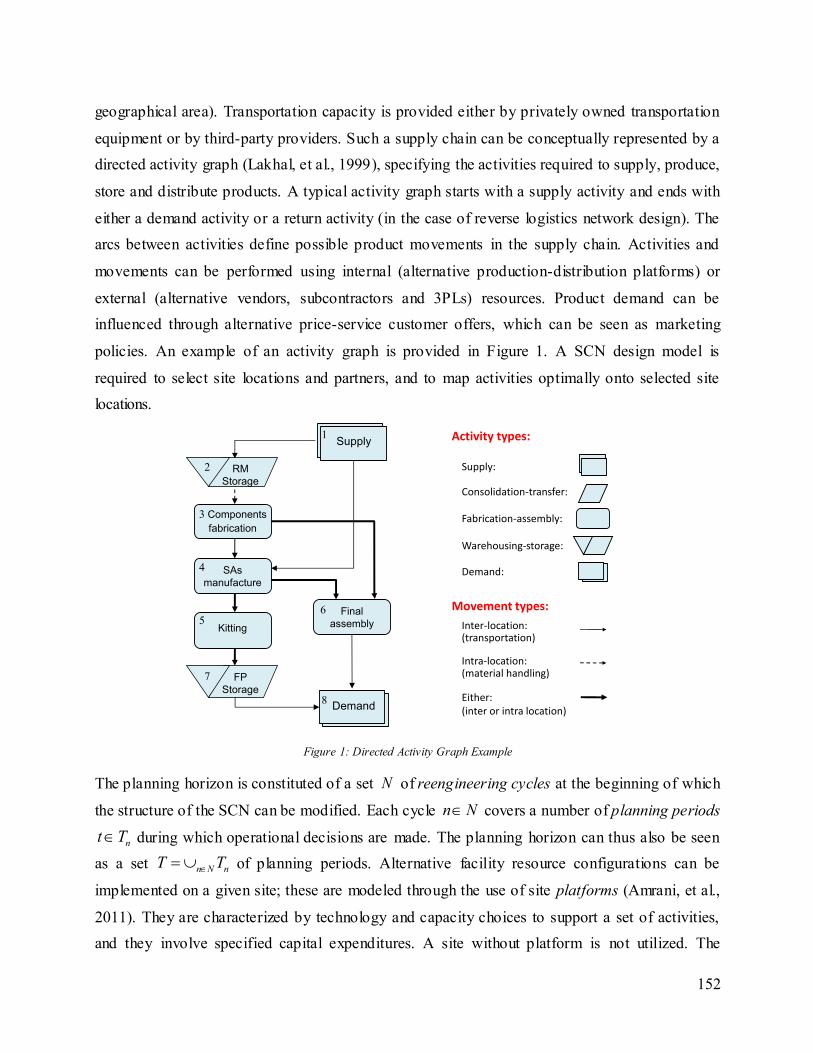
152
geographical area). Transportation capacity is provided either by privately owned transportation
equipment or by third-party providers. Such a supply chain can be conceptually represented by a
directed activity graph (Lakhal, et al., 1999), specifying the activities required to supply, produce,
store and distribute products. A typical activity graph starts with a supply activity and ends with
either a demand activity or a return activity (in the case of reverse logistics network design). The
arcs between activities define possible product movements in the supply chain. Activities and
movements can be performed using internal (alternative production-distribution platforms) or
external (alternative vendors, subcontractors and 3PLs) resources. Product demand can be
influenced through alternative price-service customer offers, which can be seen as marketing
policies. An example of an activity graph is provided in Figure 1. A SCN design model is
required to select site locations and partners, and to map activities optimally onto selected site
locations.
Figure 1: Directed Activity Graph Example
The planning horizon is constituted of a set N of reengineering cycles at the beginning of which
the structure of the SCN can be modified. Each cycle n N covers a number of planning periods
nt T during which operational decisions are made. The planning horizon can thus also be seen
as a set n N nT T of planning periods. Alternative facility resource configurations can be
implemented on a given site; these are modeled through the use of site platforms (Amrani, et al.,
2011). They are characterized by technology and capacity choices to support a set of activities,
and they involve specified capital expenditures. A site without platform is not utilized. The
Supply:
Warehousing-storage:
Demand:
Activity types:
Fabrication-assembly:
Consolidation-transfer:
Movement types:
Inter-location:(transportation)
Intra-location:(material handling)
Either: (inter or intra location)
SupplySupply
Final
assembly
SupplyDemand
FP
Storage
RM
Storage
fabrication
SAs
manufacture
Kitting
1
2
3 Components
4
56
7
8
153
platform on a site can change at the beginning of reengineering cycles to reflect opening, closing,
expansion or reorganization decisions. Platforms are also used to characterize the offers of
potential subcontractors or public warehouses. Sourcing and transportation contracts specify
prices and capacity for raw material and transportation service vendors. Demand-shaping offers
are potential offers to product-markets in terms of price, response time, fill rate, or other order
winning criteria. They influence demand and they may impose constraints on the network
structure. Individual products short-term procurement, production, inventory and shipping
decisions are aggregated into flow, activity level and inventory level decisions for product
families, demand zones and planning periods. A multi-cycle, multi-period, model is required to
address the progressively changing nature of the SCN over the strategic planning horizon (Melo,
et al., 2011).
6.2.3.2 Modeling Randomness
Rather than assuming that all the design model parameter values are known beforehand, an
explicit effort is made to account for imperfect information. Risk arises due to the temporal
separation between SCN design decision cycles and the observation of data regarding operational
parameters such as demands, prices, and costs (Mitra, et al., 2006). Rather than limiting ourselves
to the consideration of a number of representative scenarios a priori, uncertain parameters are
modeled as random variables. As a result, since some of these random variables are usually
continuous or defined over a countably infinite set of values, the set of plausible future
scenarios is infinite. To circumvent this difficulty, samples of scenarios can be generated with
Monte Carlo methods, and used to build sample average approximation (SAA) models (A.
Shapiro, 2003) and to evaluate candidate designs.
When considering a long planning horizon affected by varying economic, social and
environmental conditions, trying to estimate non-stationary stochastic processes for all random
model parameters may prove overwhelming. The approach suggested here to reduce this
complexity is to estimate probability distributions for the first period of the planning horizon
using historical data, and then to project these distributions in time with key predictors such as
inflation, energy prices, economic growth, and interest rates. For each of these predictors, several
plausible future trends may be explored; these may represent pessimistic, neutral, or optimistic
tendencies or, alternatively, more refined views of the possible evolution of the business
environment. Klibi and Martel (2011) refer to these as evolutionary paths. An evolutionary path
154
specifies a specific trend over the planning horizon for each predictor, and it has a subjectively
estimated realization probability. The trends associated to a specific evolutionary path shape the
random variables used to generate scenarios; for example, energy prices impacts transportation
costs while economic growth drives market demand. Thus, the probability functions estimated for
the operational parameters are projected over the planning horizon according to the realization of
evolutionary paths. For example, the energy prices trend associated to a specific path shapes the
probability distributions used to generate transportation costs for all planning periods. When
sampling a scenario , an evolutionary paths is first selected randomly and then parameter
values are generated using projected inverse distribution functions. The scenarios generated with
this Monte Carlo method are equiprobable (Shapiro, 2003).
Given the conditional probability modeling approach described above, and since SCN design
decisions are typically made on a rolling horizon basis, our SCN design problem can reasonably
be modeled as a two-stage stochastic program with multiple time periods (Klibi and Martel
(2011). In this program, first-stage decision variables correspond to the strategic SCN design
decisions made at the beginning of reengineering cycles n N , whereas second-stage decision
variables correspond to aggregate product flows through the resulting network arcs and activity
levels in the network nodes for planning periods t T . Once all the first-stage variables are set,
the resulting second-stage program is linear and decomposable by scenario. While using a large
number of scenarios generally results in improvement of the solution quality, it also increases the
difficulty to solve the model to optimality (Santoso, et al., 2005).
6.2.3.3 SCN Design Model
Our objective is to maximize expected economic value creation over the planning horizon as well
as to minimize downside risk using a coherent risk measure. Thus, a weighted combination of
reward and risk must be optimized. In the model proposed, the reward is the expected discounted
economic value added (EVA) of the SCN over the planning horizon. Risk aversion is captured
using the mean negative semi-deviation with respect to expected EVA. Details on this type of
risk modeling approach are found in A. Shapiro (2008). Strategic network design decisions are
related to the selection of suppliers, facility locations, facilities platform, transportation contracts,
and demand shaping offers. The model is obtained by mapping activities on potential vendors,
platforms and demand zones, and by considering possible annual product flows and inventories
over the planning horizon. The potential supply chain network thus obtained is a directed multi-
155
graph with nodes corresponding to (activity-resource) pairs and arcs to (product, origin,
destination, planning period) quadruplets. Activity level and inventory level variables are also
associated to the network nodes. The structure of the stochastic programming model to solve on a
rolling horizon basis for the SCN design problem under risk can be synthesized as follows. Let,
p
nx : Vector of binary decision variables equal to 1 when using a given facility platform on a
network site during reengineering cycle n N , and 0 otherwise.
s
nx : Vector of binary decision variables equal to 1 when selecting a given
sourcing/transportation contract for cycle n N , and 0 otherwise.
m
nx : Vector of binary decision variables equal to 1 when a given demand shaping offer is
selected for a product-market during cycle n N , and 0 otherwise.
p s m( , , )n n n nx x x x : Vector of all binary design variables for reengineering cycle n N .
f
t y : Vector of decision variables giving aggregate product flows on the network arcs in
planning period t T for scenario .
a
t y : Vector of decision variables giving aggregate activity levels (production or throughput)
of the network nodes (plants or depots) in planning period under scenario .
i
t y : Vector of decision variables giving aggregate inventory levels in the nodes of the
network at the end of planning period t T under scenario .
f a i( , , )t t t t y y y y : Vector of all continuous operational decision variables for
period t T under scenario .
f
t p : Vector of the unit prices paid for the delivery of the products associated to the flows
f
t y under scenario .
t c : Vector of the unit variable costs associated to the elements of activity vector ( )t y
under scenario .
te : Vector of the capital expenditures incurred in planning period t for the elements of
design vector ( )n tx (n(t) denotes the cycle n including planning period t).
tEVA : Economic value added by the SCN for planning period t T under scenario .
: Discount rate used by the company, based on its weighted average cost of capital
(WACC).
t T
156
c
tb : Vector of the capacity provided in period t T by the platform, sourcing and
transportation resources/contracts associated to the elements of design variables vector
p s
( ) ( )( , )n t n tx x .
d
t b : Vector of the demand in period t T under the demand shaping offer associated to the
elements of design variable vector ( )
m
n tx for scenario .
c d( , )t t t b b b : Vector of all capability parameter values associated to design vector ( )n tx
for period t T , under scenario .
: Parameter weighting the mean negative semi-deviation in the objective function
( 0 ).
In some formulations, complementary change-of-state binary variables are also defined to
facilitate the modeling of change-of-state expenses. Using this notation, the typical multi-cycle
two-stage stochastic program formulated for SCN design problems is:
max min 0E V E V E V
, (1)
subject to
f f
( ), [ ]
(1 )
t
t t t t t t n ttt T
EVAV EVA
p y c y e x (2)
p p
1 1n n n n n U x W x h
n N (3)
n nXx
n N (4)
( )t t t n t A y b x
,t T (5)
1( , )
t t tY
y y
,t T (6)
where 1nU , n
W and tA are parameter matrices, n
h is a parameter vector, nX is the set of
feasible designs specified by local cycle n constraints, and tY is an activity level feasibility
set for planning period t under scenario . The objective function (1) maximizes expected
value creation over the planning horizon across all scenarios, damped by the mean negative semi-
deviation across all scenarios. Eppen, Martin and Schrage (1989) provide a thorough discussion
of the sensitivity analysis to perform in a SCN design context when downside risk is considered.
Constraints (3) ensure that platforms are changed coherently from a reengineering cycle (p
1nx ) to
the next (p
nx ). Constraints (4) include additional cycle dependent constraints required to make
sure that design options are properly selected. For example, during a cycle, one cannot operate
157
more than one platform on a site or select more than one demand shaping offer for a product-
market. Constraints (5) specify the activity level restrictions imposed in period t T by the
capabilities provided by the selected design ( )n tx . These are mainly production-warehousing
capacity constraints on a
t y , storage capacity constraints on i
t y , as well as vendor
capacity, transportation capacity and potential demand constraints on f
t y . Finally, (6)
includes mainly flow conservation constraints on t y , and accounting constraints to calculate
end-of-period inventories i
t y from initial inventories i
1t y and relevant inflows/outflows
in f a( , )t t y y .
Note that all the constraints of the streamlined formulation presented are linear. However, when
concave inventory-throughput functions (Ballou, 1992) are used to reflect economies of scale in
cycle and safety stocks, non- linear terms are introduced in (2) and (5). The model is then much
more difficult to solve. The formulation presented captures the main elements of deterministic
multi-cycles SCN design models such as those proposed by Martel (2005), Thanh (2008),
M'Barek, et al. (2010) and Carle, et al. (2012a). It also indicates how they are converted in a
stochastic programming with recourse model.
As it stands, the stochastic program formulated can rarely be solved because there is usually an
infinite number of scenarios in . As indicated previously, to circumvent this difficulty, several
samples , 1,...,m
i i I , of m scenarios can be generated with Monte Carlo methods, and
used to build sample average approximation (SAA) models. When this is done, for a given
sample i, the objective function (1) becomes
1 1 1
max min 0m m mi i i
V V Vm m m
,
(7)
and constraints (5) and (6) are defined for the scenarios in m
i instead of . By solving the
resulting deterministic program, as much as I distinct candidate designs ( )i i
n n NX x can be
obtained. One must then select one of these candidate designs. To evaluate the designs, a separate
sample of scenarios M , with M m , is generated. The value iV X , of the designs
, 1,...,i i IX , is then calculated for each scenario M . This value is provided by the solution
of the second-stage linear program obtained by setting ( ) i
n n N x X in the previous model and by
considering a single scenario M at the time (A. Shapiro (2003). Using these values, one can
then estimate M
iE V
X , and min 0M M
i iE V E V
X X, , , , for , 1,...,i i IX
, and select the best design. Note that the downside risk term in (7) complicates the solution of
158
SAA models significantly. For this reason, it is often neglected, i.e. the decision-maker is
assumed to be risk-neutral. The SAA model then becomes a standard MIP (Mixed Integer
Program).
6.2.4 Solution Approach
The SAA programs obtained for our SCN design model are extremely large, even when scenario
samples of moderate size are used, and they are very difficult to solve with state-of-the-art
commercial MIP solvers such as CPLEX and Gurobi. Classical metaheuristics such as tabu
search and genetic algorithms are typically ill- suited to handle the large number of continuous
variables contained in the aforementioned models. Thus, the development of a hybrid
metaheuristic, which makes effective use of both heuristics and exact methods, seems
appropriate. To solve large instances of our stochastic optimization problem, we use CAT, an
agent-based metaheuristic proposed to solve deterministic instances of the SCN design problem
(Carle, et al., 2012a) and adapt it to stochastic problems. A thorough discussion on CAT and
some implementation guidelines are provided in (Carle, Martel, & Zufferey, 2012b). The strategy
used for creating sub-models is presented in section 3.1, while the adaptations required to solve
stochastic models are explained in section 3.2. The actual agents and algorithms used are
explained in section 3.3.
6.2.4.1 CAT Structure and Sub-Models
CAT makes effective use of distributed decision making principles (Schneeweiss, 2003) and the
multi-agent paradigm. Using this approach, the SCN design problem is partitioned using logical
views rather than the mathematical properties of the design model. For instance, a firm’s SCN
can be divided into sales territories, each encompassing several states or geographical regions;
alternatively, resource deployment decisions (supplier selection, facility location, etc.) may be
addressed separately. Using the insights provided by dimensional views, the complete SCN
design model is divided into several, not necessarily mutually-exclusive, sub-models; each of
these sub-models is associated to a sub-problem and it is solved using a specific algorithm
(heuristic or exact method implemented through branch-and-cut solvers). The solutions to these
sub-models (called partial solutions) are then integrated into solutions to the complete model by
agents. For our SCN design problem, three dimensional views are used to develop sub-models:
159
The resource-based view refers to the interrelations between different supply chain decisions
such as purchasing and vendor selection decisions, production-distribution facility location
and platform selection decisions, as well as demand shaping offer choices. Each of these
decision types, with the associated product flow and activity level variables, provides a
resource-based sub-model.
The spatial dimension refers to the geographical positioning of business entities such as sales
territories, national divisions or subsidiaries. One can then divide the problem into several
spatial sub-models.
The scenario dimension refers to the wait-and-see (second-stage) decisions in our stochastic
design model, and the associated variables and constraints. Depending on the scenario sample
considered and the values of the model parameters for each of these scenarios, different
second-stage sub-models are produced.
The task of solving a given sub-model is then assigned to a specific optimization agent. An agent
is an independent piece of software that has its own algorithms, memory structures as well as
rules for deciding when to work, what to work on and when to stop working. An agent may use
several algorithms and strategies, but a given agent always works on a single model, whether it is
the complete model or one of the sub-models. Although agents work in parallel, a specific agent
works sequentially, using one algorithm to build or improve one solution at a time, since using
parallel algorithms could hamper other agents’ access to processor time and memory. Some
agents use mixed- integer programming (MIP) solvers while others use generic MIP heuristics or
metaheuristics, making CAT an effective approach to combine several optimization strategies.
CAT is composed of a blackboard, utility agents and optimization agents. The blackboard acts as
a memory and a hub for all communications, as well as holding the repository of all solutions (to
the model and all sub-models). Optimization agents are grouped into four types depending on
their role. Construction agents create new solutions from scratch. Improvement agents take
existing solutions and modify them to improve their quality. Destruction agents remove
unwanted solutions from the repository. Finally, integration agents combine high-quality
solutions from two or more sub-models into solutions to the complete design problem. Utility
agents provide functionalities used by all agents, such as building model files for solvers,
scenario generation and solution evaluation. The scenario generator creates scenarios for the
complete model as well as sub-scenarios to evaluate solutions to sub-models.
160
6.2.4.2 Solving Stochastic SCN Design Problems with CAT
A number of modeling and algorithmic strategies can be used to effectively solve stochastic
problems with CAT. A straightforward strategy is to use scenario samples of different size
depending on the difficulty of the problem address by an agent. As sub-models are much smaller
and easier to solve than the complete optimization model, agents working on sub-models are able
to use a larger number of scenarios than those working on the complete model, resulting in higher
solution quality. Each agent then works using the number of scenarios giving an acceptable trade-
off between solution quality and model solvability.
Another option is to use different sets of scenarios to generate different candidate solutions, as
typically done with the SAA approach. In particular, agents can use quick constructive heuristics
(such as greedy approaches) to provide a feasible solution, and then use the same heuristic with a
different set of scenarios to hopefully provide a different solution. A similar strategy can be used
in variable fixing heuristics: variables which have the same values in solutions generated with
different algorithms and/or different sets of scenarios are fixed first.
The parallel and distributed nature of agents is also exploited in solution evaluation. Most
optimization agents require speed and thus have to evaluate candidate solutions over a relatively
small number of scenarios. The solution evaluation agents can use a much larger set of scenarios
to provide a more precise evaluation of the quality of solutions and to compute appropriate risk
measures. This extensive solution evaluation process is computationally expensive as it requires
solving a large number of second-stage programs, but it can easily be tackled by using several
solution evaluation agents in parallel.
6.2.4.3 Agents and Algorithms
The CAT implementation proposed to solve SCN design problems includes 15 different
optimization agents. Table 1 presents the agents’ most important characteristics: name, type (“C”
for construction, “I” for improvement, “D” for destruction, “N” for integration and “E” for
evaluation), the number of heuristics the agent possesses, whether the implementation hosts a
single copy of the agents (S) or several copies that execute in parallel (P), and whether the agents
use a single scenario (1) or multiple scenarios (M). Since the number of heuristics used is rather
large, it is not possible to provide a pseudo-code of each of them. Instead, a general outlook of
the approach used by each agent is provided, along with references to similar heuristics. All
heuristics and agents are coded in C# and VB.NET 2008, and each agent is an executable
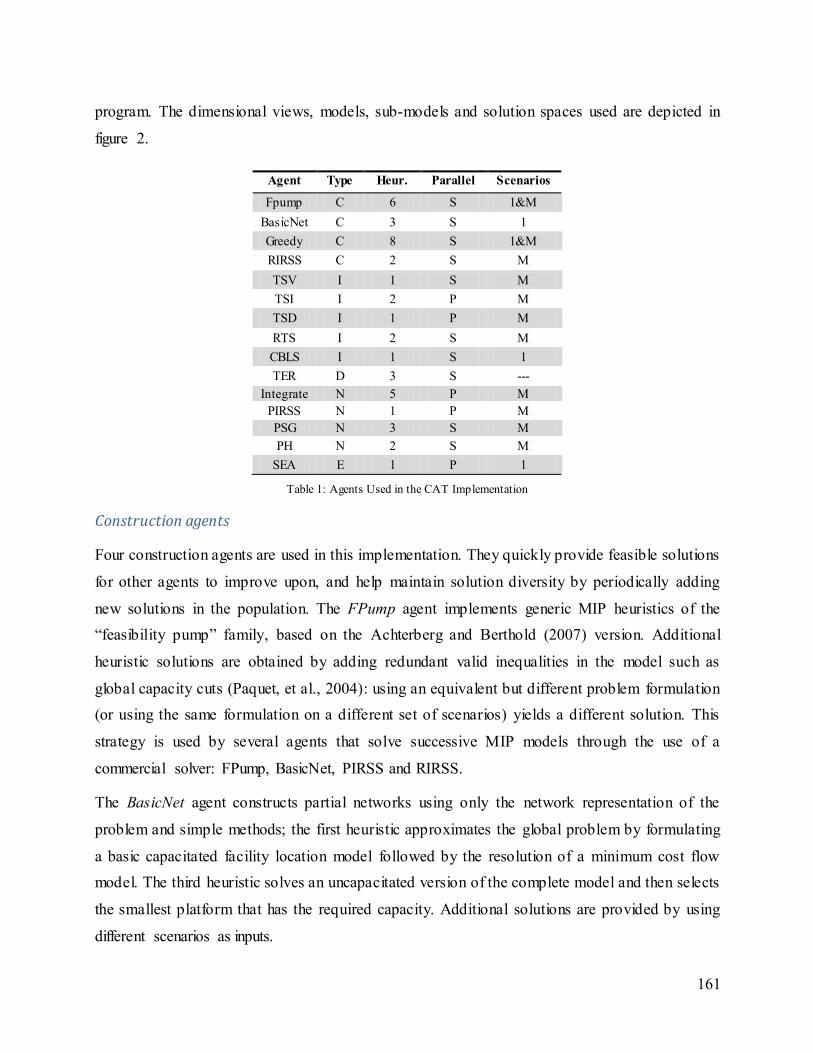
161
program. The dimensional views, models, sub-models and solution spaces used are depicted in
figure 2.
Table 1: Agents Used in the CAT Implementation
Construction agents
Four construction agents are used in this implementation. They quickly provide feasible solutions
for other agents to improve upon, and help maintain solution diversity by periodically adding
new solutions in the population. The FPump agent implements generic MIP heuristics of the
“feasibility pump” family, based on the Achterberg and Berthold (2007) version. Additional
heuristic solutions are obtained by adding redundant valid inequalities in the model such as
global capacity cuts (Paquet, et al., 2004): using an equivalent but different problem formulation
(or using the same formulation on a different set of scenarios) yields a different solution. This
strategy is used by several agents that solve successive MIP models through the use of a
commercial solver: FPump, BasicNet, PIRSS and RIRSS.
The BasicNet agent constructs partial networks using only the network representation of the
problem and simple methods; the first heuristic approximates the global problem by formulating
a basic capacitated facility location model followed by the resolution of a minimum cost flow
model. The third heuristic solves an uncapacitated version of the complete model and then selects
the smallest platform that has the required capacity. Additional solutions are provided by using
different scenarios as inputs.
Agent Type Heur. Parallel Scenarios
Fpump C 6 S 1&M
BasicNet C 3 S 1
Greedy C 8 S 1&M
RIRSS C 2 S M
TSV I 1 S M
TSI I 2 P M
TSD I 1 P M
RTS I 2 S M
CBLS I 1 S 1
TER D 3 S ---
Integrate N 5 P M
PIRSS N 1 P M
PSG N 3 S M
PH N 2 S M
SEA E 1 P 1
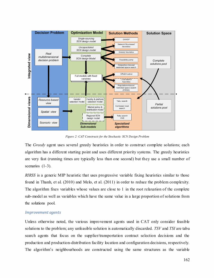
162
Figure 2: CAT Constructs for the Stochastic SCN Design Problem
The Greedy agent uses several greedy heuristics in order to construct complete solutions; each
algorithm has a different starting point and uses different priority systems. The greedy heuristics
are very fast (running times are typically less than one second) but they use a small number of
scenarios (1-3).
RIRSS is a generic MIP heuristic that uses progressive variable fixing heuristics similar to those
found in Thanh, et al. (2010) and Melo, et al. (2011) in order to reduce the problem complexity.
The algorithm fixes variables whose values are close to 1 in the root relaxation of the complete
sub-model as well as variables which have the same value in a large proportion of solutions from
the solutions pool.
Improvement agents
Unless otherwise noted, the various improvement agents used in CAT only consider feasible
solutions to the problem; any unfeasible solution is automatically discarded. TSV and TSI are tabu
search agents that focus on the supplier/transportation contract selection decisions and the
production and production-distribution facility location and configuration decisions, respectively.
The algorithm’s neighbourhoods are constructed using the same structures as the variable
163
neighbourhood search heuristic of Amrani et al. (2011). As advised in Sörensen (2002), a small
sample of scenarios (5-10) are used during the candidate move evaluation phase, in order to
speed up the search process, while the move selected at the end of iteration is evaluated using a
larger sample (25-50) of scenarios. TSD also uses tabu search but focuses its work on distribution
facility location, configuration and marketing policy selection decisions. Since candidate moves
evaluation is significantly longer for stochastic problems than for the deterministic version
presented in Carle, et al. (2012a), two copies of the TSI and TSD agents are run in parallel, each
working to improve a different solution.
RTS uses a local search which operates on all decisions relevant to a small portion of the territory
covered by the company’s supply chain network. While one heuristic uses a static division of the
territory corresponding to national divisions or sales territories, the second heuristic divides the
supply chain dynamically in zones constructed by the agent itself. The size of the zones included
varies according to instance size but typically covers about 20% of the SCN. Diversification is
made by penalizing strategic options that are selected most often, in order to provide incentive to
explore new solution spaces. Candidate move evaluation and selected solution evaluation are
made respectively with smaller and larger scenario sample sizes, with the same parameters as
agents TSI and TSD.
CBLS uses a local search heuristic whose main objective is to explore new solution spaces. As
such, it constructs a special exclusion list which is composed of the strategic options that are used
in the majority of solutions in the population. It also forces the solution to include a small number
of strategic options that are least used in the current population. Although the solutions it yields
are not of exceptional quality, it is very effective for diversification purposes.
Integration agents
Integration agents create new solutions by combining different features from several solutions in
the population, instead of working from a single solution. The Integrate agent integrates either
resource-based or spatial partial solutions from different sub-models to form solutions to the
complete model. To that purpose, it uses six heuristics grouped into two categories. Heuristics of
the first category combine features from solutions to different resource-based sub-models into a
single solution to the complete model. For example, vendor selection options from a solution are
integrated with facility configurations and demand shaping decisions from another solution. The
same strategy is applied to solutions to spatial sub-models. Sequential improvements are then
164
made until a strong local optimum is reached. Since it is trivial to assemble solutions from
different scenarios, a heuristic is not required. The second category of heuristics uses solution
combination heuristics inspired from the crossover operators in genetic and memetic algorithms
(Altiparmak, et al., 2009).
The PIRSS agent integrates one solution to the complete models with one or more partial of
complete solutions. It effectively models the solution space formed by the union of two or more
input solutions as a MIP, and then solves the integration sub-model using CPLEX. Binary
variables equal to 1 in all the input solutions are fixed in the model, while binary variables that
differ in value between input solutions are left unfixed for the model to solve. This effectively
produces a sub-model that is a restriction of the complete optimization model. A computation
time limit is used so the agent doesn’t spend too much time on a single integration. If the time
limit is reached, the best found solution is recorded. The first heuristic used integrates two
solutions to the complete model while the second integrates one solution to the complete model
with two or more solutions from resource-based sub-models.
PSG uses a GRASP metaheuristic to build solutions to the complete model. Each of the three
heuristics starts with a solution of a resource-based sub-model and then completes it through a
multi-start improvement procedure.
PH aims to produce high-quality solutions to a specific sub-model by combining the features of
solutions common to several solutions. It uses a heuristic strategy inspired from progressive
hedging techniques (Rockafellar & Wets, 1991) that was recently proposed to solve stochastic
multi-commodity network design problems (Crainic, et al., 2011). Two variants are applied to the
distribution network design sub-model as well as the regional SCN design sub-models. The
heuristic solves a series of sub-models with a small number of scenarios (5-10) using CPLEX.
The coefficients associated to binary variables in the objective function are iteratively modified
as to reach a consensus design, and the sub-models are solved again. When two iterations are
performed with minimal coefficient modification, the variables that are consensual in all sub-
models are fixed (a strategy called slamming by Badilla-Veliz, et al. (2012)), and a larger number
of scenarios is used (10-20) to improve the solution. This is done repeatedly until all variables
have been fixed.
165
Evaluation agents
Given a number of selected strategic options and a set of scenarios, the SEA agent optimizes the
supply chain network flow model across all scenarios and time periods. In other words, SEA
solves the second-stage program of our stochastic model. Since this model is fully decomposable
by scenario, it effectively solves a series of linear programs. In order to provide a good evaluation
of solution quality, a large sample of scenarios (typically 1000) is used. A SEA agent always
selects the solution that has the best objective function value among those that have not been
through detailed evaluation yet. A precise evaluation of a solution’s quality serves two purposes.
First, optimization agents need feedback on the quality of the solution they yield, as well as on
the quality of estimation provided by the small set of scenarios they use for candidate solution
evaluation. Second, when selecting a new solution to work upon, improvement and integration
agents need an evaluation that is as accurate as possible. In order to spend more resources on
evaluation than on solution generation, only those solutions which are above the median of the
population are evaluated by the SEA agents. In particular, finding the right number of solution
evaluation agents (SEA) to use in parallel is important; in our implementation, two copies of the
agent run in parallel.
Destruction agent
The role of destruction agents is to remove unwanted solutions from the population in order to
keep its size in check. Since deleting solutions is a lot faster than construction or improvement, a
single destruction agent is sufficient. Solutions created by a constructive heuristic are protected
from destruction until they have been improved by at least two improvement agents, as is the best
solution in the population. Three decision rules are used for deletion:
1. Destroy the solution that has the lowest objective function value;
2. Destroy a solution at random that is in the lowest half among all solutions for both
expected value and downside risk;
3. Among the two solutions that are the most similar, destroy the solution that has the lowest
solution quality.
Solutions that have not yet been through detailed evaluation by SEA agents are not available for
deletion through the application of rule #2 since the estimation of downside risk provided by
optimization agents is not precise enough.
166
6.2.5 Computational Results
Solving stochastic SCN design models through CAT yields four potential advantages over the
solution of sample average approximation (SAA) programs with MIP solvers:
1. Superior performance of CAT compared to SAA;
2. The ability to solve larger instances;
3. The capability to take into account nonlinear inventory-throughput functions;
4. The capacity to consider downside risk directly in the solution of models.
In order to validate and assess whether these benefits are real, different benchmark SCN design
problem instances were generated. These instances represent a typical B2B company
manufacturing and selling products through the United States. Product demands and prices,
transportation costs as well as the fixed and variable costs of each platform, vendor offer and
transportation options are based on realistic parameter value ranges found in the Usemore case
(Ballou, 1992). Market demands for each product are assumed to follow a log-normal distribution
in order to generate non-negative values. According to several authors (Kamath & Pakkala, 2002;
Santoso, et al., 2005), log-normal distributions are well suited for modelling product demands.
Other parameters such as costs and product prices are assumed to follow a Normal distribution.
Five different network structures are used, each comprising different cities from among the 100
US largest metropolitan areas. A first set of 20 instances was initially generated to develop and
test the CAT system. In order to avoid the risk of developing algorithms that are over-tuned to
specific instances, this set was discarded and the results reported below are on a new set of
instances; that is, the results reported are those of the first run of CAT on each of these instances.
According to Birattari (2009), this “N-instance, 1 run per instance” approach is particularly well
suited to compare different optimization algorithms. For testing purposes, four sets of 30
instances of increasing size were generated; they are presented in
Table 2. In addition to the increased number of sites considered, instances from SET-3 and SET-4
have three potential upgrade platforms available for each alternative platform considered. This
considerably increases the number of binary variables present in the model. All the experiments
were performed on a dual 2.66 GHz 64-bit Intel Xeon® computer with 64 GB of RAM.
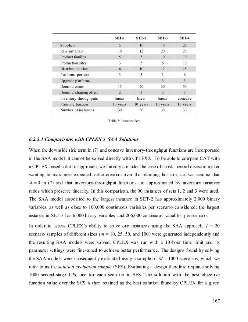
167
Table 2: Instance Sets
6.2.5.1 Comparisons with CPLEX’s SAA Solutions
When the downside risk term in (7) and concave inventory-throughput functions are incorporated
in the SAA model, it cannot be solved directly with CPLEX®. To be able to compare CAT with
a CPLEX-based solution approach, we initially consider the case of a risk-neutral decision maker
wanting to maximize expected value creation over the planning horizon, i.e. we assume that
0 in (7) and that inventory-throughput functions are approximated by inventory turnover
ratios which preserve linearity. In this comparison, the 90 instances of sets 1, 2 and 3 were used.
The SAA model associated to the largest instance in SET-2 has approximately 2,000 binary
variables, as well as close to 100,000 continuous variables per scenario considered; the largest
instance in SET-3 has 6,000 binary variables and 206,000 continuous variables per scenario.
In order to assess CPLEX’s ability to solve our instances using the SAA approach, I = 20
scenario samples of different sizes (m = 10, 25, 50, and 100) were generated independently and
the resulting SAA models were solved. CPLEX was run with a 10-hour time limit and its
parameter settings were fine-tuned to achieve better performance. The designs found by solving
the SAA models were subsequently evaluated using a sample of M = 1000 scenarios, which we
refer to as the solution evaluation sample (SES). Evaluating a design therefore requires solving
1000 second-stage LPs, one for each scenario in SES. The solution with the best objective
function value over the SES is then retained as the best solution found by CPLEX for a given
SET-1 SET-2 SET-3 SET-4
Suppliers 5 10 10 20
Raw materials 10 12 20 20
Product families 5 5 10 10
Production sites 3 5 6 10
Distribution sites 6 10 12 15
Platforms per site 3 3 3 6
Upgrade platforms --- --- 3 3
Demand zones 15 20 30 50
Demand shaping offers 2 3 3 3
Inventory-throughputs linear linear linear concave
Planning horizon 10 years 10 years 10 years 10 years
Number of instances 30 30 30 30
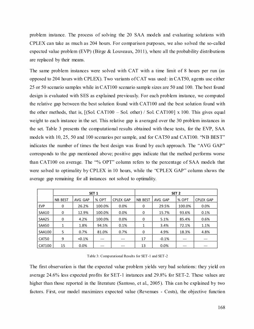
168
problem instance. The process of solving the 20 SAA models and evaluating solutions with
CPLEX can take as much as 204 hours. For comparison purposes, we also solved the so-called
expected value problem (EVP) (Birge & Louveaux, 2011), where all the probability distributions
are replaced by their means.
The same problem instances were solved with CAT with a time limit of 8 hours per run (as
opposed to 204 hours with CPLEX). Two variants of CAT was used: in CAT50, agents use either
25 or 50 scenario samples while in CAT100 scenario sample sizes are 50 and 100. The best found
design is evaluated with SES as explained previously. For each problem instance, we computed
the relative gap between the best solution found with CAT100 and the best solution found with
the other methods, that is, [(Sol. CAT100 – Sol. other) / Sol. CAT100] x 100. This gives equal
weight to each instance in the set. This relative gap is averaged over the 30 problem instances in
the set. Table 3 presents the computational results obtained with these tests, for the EVP, SAA
models with 10, 25, 50 and 100 scenarios per sample, and for CAT50 and CAT100. “NB BEST”
indicates the number of times the best design was found by each approach. The “AVG GAP”
corresponds to the gap mentioned above; positive gaps indicate that the method performs worse
than CAT100 on average. The “% OPT” column refers to the percentage of SAA models that
were solved to optimality by CPLEX in 10 hours, while the “CPLEX GAP” column shows the
average gap remaining for all instances not solved to optimality.
SET 1 SET 2
NB BEST AVG GAP % OPT CPLEX GAP NB BEST AVG GAP % OPT CPLEX GAP
EVP 0 26.2% 100.0% 0.0% 0 29.5% 100.0% 0.0%
SAA10 0 12.9% 100.0% 0.0% 0 15.7% 93.6% 0.1%
SAA25 0 4.2% 100.0% 0.0% 0 5.1% 85.4% 0.6%
SAA50 1 1.8% 94.5% 0.1% 1 3.4% 72.1% 1.1%
SAA100 5 0.7% 81.0% 0.7% 0 4.9% 18.3% 4.8%
CAT50 9 <0.1% --- --- 17 -0.1% --- ---
CAT100 15 0.0% --- --- 13 0.0% --- ---
Table 3: Computational Results for SET-1 and SET-2
The first observation is that the expected value problem yields very bad solutions: they yield on
average 24.6% less expected profits for SET-1 instances and 29.8% for SET-2. These values are
higher than those reported in the literature (Santoso, et al., 2005). This can be explained by two
factors. First, our model maximizes expected value (Revenues - Costs), the objective function
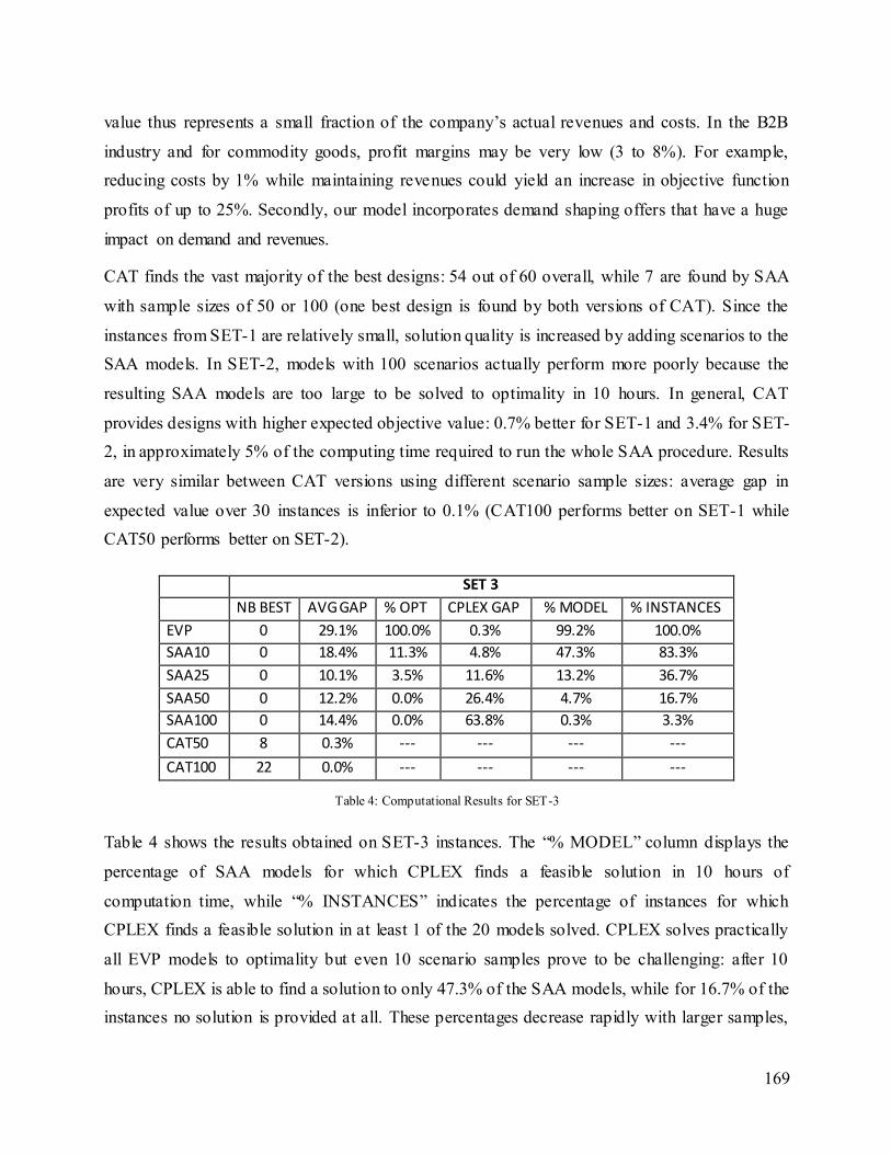
169
value thus represents a small fraction of the company’s actual revenues and costs. In the B2B
industry and for commodity goods, profit margins may be very low (3 to 8%). For example,
reducing costs by 1% while maintaining revenues could yield an increase in objective function
profits of up to 25%. Secondly, our model incorporates demand shaping offers that have a huge
impact on demand and revenues.
CAT finds the vast majority of the best designs: 54 out of 60 overall, while 7 are found by SAA
with sample sizes of 50 or 100 (one best design is found by both versions of CAT). Since the
instances from SET-1 are relatively small, solution quality is increased by adding scenarios to the
SAA models. In SET-2, models with 100 scenarios actually perform more poorly because the
resulting SAA models are too large to be solved to optimality in 10 hours. In general, CAT
provides designs with higher expected objective value: 0.7% better for SET-1 and 3.4% for SET-
2, in approximately 5% of the computing time required to run the whole SAA procedure. Results
are very similar between CAT versions using different scenario sample sizes: average gap in
expected value over 30 instances is inferior to 0.1% (CAT100 performs better on SET-1 while
CAT50 performs better on SET-2).
SET 3
NB BEST AVG GAP % OPT CPLEX GAP % MODEL % INSTANCES
EVP 0 29.1% 100.0% 0.3% 99.2% 100.0%
SAA10 0 18.4% 11.3% 4.8% 47.3% 83.3%
SAA25 0 10.1% 3.5% 11.6% 13.2% 36.7%
SAA50 0 12.2% 0.0% 26.4% 4.7% 16.7%
SAA100 0 14.4% 0.0% 63.8% 0.3% 3.3%
CAT50 8 0.3% --- --- --- ---
CAT100 22 0.0% --- --- --- ---
Table 4: Computational Results for SET-3
Table 4 shows the results obtained on SET-3 instances. The “% MODEL” column displays the
percentage of SAA models for which CPLEX finds a feasible solution in 10 hours of
computation time, while “% INSTANCES” indicates the percentage of instances for which
CPLEX finds a feasible solution in at least 1 of the 20 models solved. CPLEX solves practically
all EVP models to optimality but even 10 scenario samples prove to be challenging: after 10
hours, CPLEX is able to find a solution to only 47.3% of the SAA models, while for 16.7% of the
instances no solution is provided at all. These percentages decrease rapidly with larger samples,
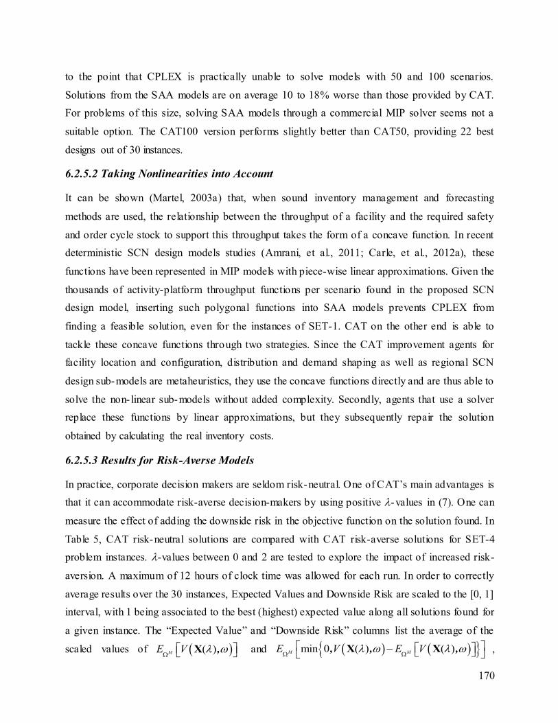
170
to the point that CPLEX is practically unable to solve models with 50 and 100 scenarios.
Solutions from the SAA models are on average 10 to 18% worse than those provided by CAT.
For problems of this size, solving SAA models through a commercial MIP solver seems not a
suitable option. The CAT100 version performs slightly better than CAT50, providing 22 best
designs out of 30 instances.
6.2.5.2 Taking Nonlinearities into Account
It can be shown (Martel, 2003a) that, when sound inventory management and forecasting
methods are used, the relationship between the throughput of a facility and the required safety
and order cycle stock to support this throughput takes the form of a concave function. In recent
deterministic SCN design models studies (Amrani, et al., 2011; Carle, et al., 2012a), these
functions have been represented in MIP models with piece-wise linear approximations. Given the
thousands of activity-platform throughput functions per scenario found in the proposed SCN
design model, inserting such polygonal functions into SAA models prevents CPLEX from
finding a feasible solution, even for the instances of SET-1. CAT on the other end is able to
tackle these concave functions through two strategies. Since the CAT improvement agents for
facility location and configuration, distribution and demand shaping as well as regional SCN
design sub-models are metaheuristics, they use the concave functions directly and are thus able to
solve the non- linear sub-models without added complexity. Secondly, agents that use a solver
replace these functions by linear approximations, but they subsequently repair the solution
obtained by calculating the real inventory costs.
6.2.5.3 Results for Risk-Averse Models
In practice, corporate decision makers are seldom risk-neutral. One of CAT’s main advantages is
that it can accommodate risk-averse decision-makers by using positive -values in (7). One can
measure the effect of adding the downside risk in the objective function on the solution found. In
Table 5, CAT risk-neutral solutions are compared with CAT risk-averse solutions for SET-4
problem instances. -values between 0 and 2 are tested to explore the impact of increased risk-
aversion. A maximum of 12 hours of clock time was allowed for each run. In order to correctly
average results over the 30 instances, Expected Values and Downside Risk are scaled to the [0, 1]
interval, with 1 being associated to the best (highest) expected value along all solutions found for
a given instance. The “Expected Value” and “Downside Risk” columns list the average of the
scaled values of ( ) ME V
X , and min 0 ( ) ( )M ME V E V
X X, , , ,
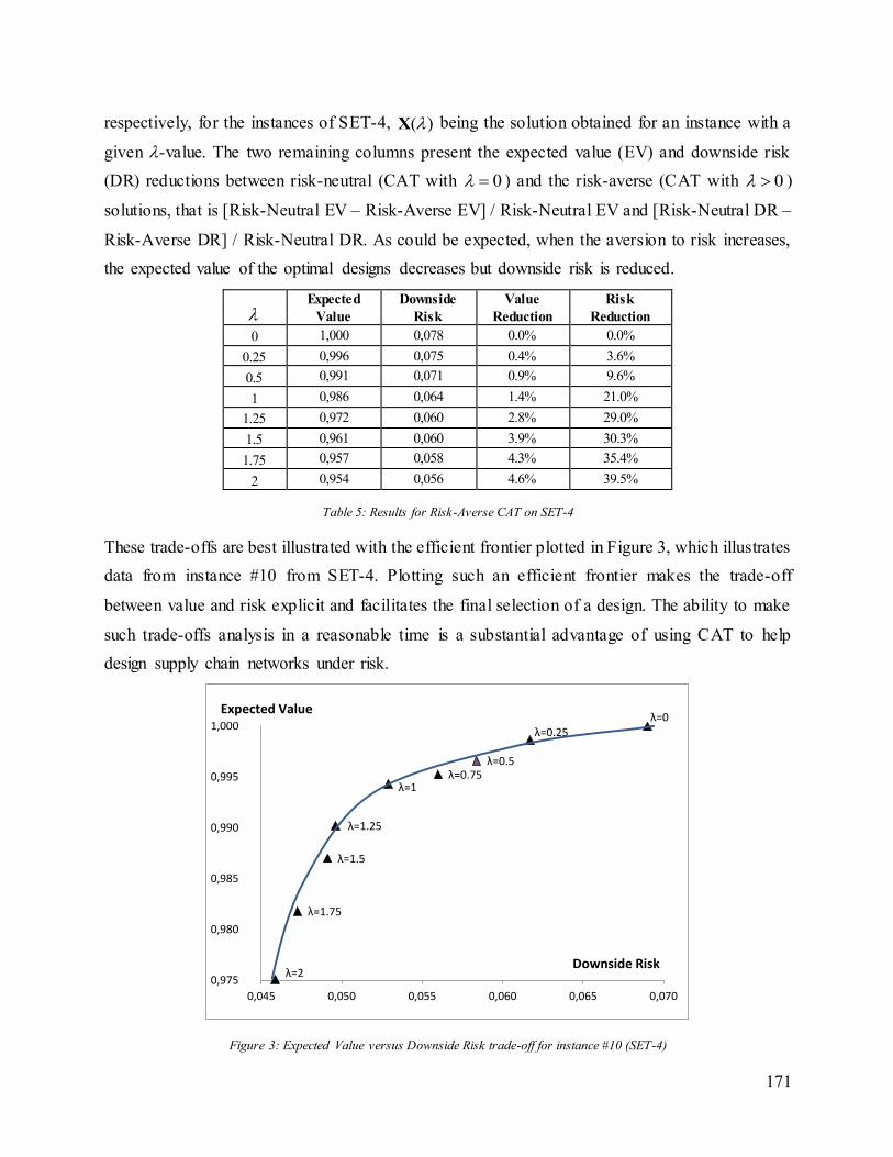
171
respectively, for the instances of SET-4, ( )X being the solution obtained for an instance with a
given -value. The two remaining columns present the expected value (EV) and downside risk
(DR) reductions between risk-neutral (CAT with 0 ) and the risk-averse (CAT with 0 )
solutions, that is [Risk-Neutral EV – Risk-Averse EV] / Risk-Neutral EV and [Risk-Neutral DR –
Risk-Averse DR] / Risk-Neutral DR. As could be expected, when the aversion to risk increases,
the expected value of the optimal designs decreases but downside risk is reduced.
Expected
Value
Downside
Risk
Value
Reduction
Risk
Reduction
0 1,000 0,078 0.0% 0.0%
0.25 0,996 0,075 0.4% 3.6%
0.5 0,991 0,071 0.9% 9.6%
1 0,986 0,064 1.4% 21.0%
1.25 0,972 0,060 2.8% 29.0%
1.5 0,961 0,060 3.9% 30.3%
1.75 0,957 0,058 4.3% 35.4%
2 0,954 0,056 4.6% 39.5%
Table 5: Results for Risk-Averse CAT on SET-4
These trade-offs are best illustrated with the efficient frontier plotted in Figure 3, which illustrates
data from instance #10 from SET-4. Plotting such an efficient frontier makes the trade-off
between value and risk explicit and facilitates the final selection of a design. The ability to make
such trade-offs analysis in a reasonable time is a substantial advantage of using CAT to help
design supply chain networks under risk.
Figure 3: Expected Value versus Downside Risk trade-off for instance #10 (SET-4)
λ=0λ=0.25
λ=0.5λ=0.75
λ=1
λ=1.25
λ=1.5
λ=1.75
λ=2 0,975
0,980
0,985
0,990
0,995
1,000
0,045 0,050 0,055 0,060 0,065 0,070
Expected Value
Downside Risk
172
6.2.6 Conclusion
This paper proposed a modeling approach for stochastic network design problems. The approach
integrates several modeling concepts previously proposed in the literature and adapts them to a
stochastic business environment. We also present a Collaborative Agent-Team (CAT)
metaheuristic that is capable of solving these large and complex stochastic op timization
problems. Required CAT constructs and the algorithms used by the agents were described.
Furthermore, by using a metaheuristic such as CAT, one is not forced to use linear constraints
and objectives (or to approximate nonlinearities by piecewise linear functions). This is especially
important for stochastic models where risk functions are not linear by nature. This opens up new
modeling opportunities. Furthermore, the CAT metaheuristic can easily be extended and
improved by adding new agents as needed.
Computational results made over 4 sets of 30 realistic test problem instances each show that CAT
is able to solve large instances. One run of CAT is usually sufficient to find better designs than a
SAA procedure using 20 scenario samples that takes 25 times longer. CAT is also able to handle
large problem sizes, up to several million variables, while SAA-CPLEX performance decreases
on larger instances. Our approach is also able to assist risk-averse decision makers by
incorporating a Downside Risk component into the objective function, allowing to find the design
that best suits the decision maker’s risk attitude. Furthermore, while using SAA models, selecting
the appropriate sample scenario size is important to reach acceptable designs, while CAT is more
resilient in this matter by yielding comparable results for different sample sizes.
This work could be extended in two ways. First, this model considered only standard fluctuations
in the business environment. Additional effort would be required to incorporate disruption risk
issues (catastrophes, deliberate sabotage, closure of a key supplier, etc.) in the model. Resilient
SCN design methodologies exist (Klibi & Martel, 2012), but so far they have been applied to
simpler SCN design models than the one proposed in this paper. Lastly, even CAT is limited in
its ability to solve very large models (100+ million variables) by the time required to so lve some
sub-models through the use of solvers. Additional effort should be invested to incorporate
decomposition techniques into these agents so that very large supply chain networks can be
optimized.
173
6.2.7 References
Achterberg, T., & Berthold, T. (2007). Improving the Feasibility Pump. Discrete Optimization, 4, 77-86.
Altiparmak, F., Gen, M., Lin, L., & Karaoglan, I. (2009). A steady-state genetic algorithm for multi-product supply chain network design. Computers & Industrial Engineering, 56, 521-537.
Amrani, H., Martel, A., Zufferey, N., & Makeeva, P. (2011). A variable neighborhood search heuristic for the design of multicommodity production-distribution networks with alternative facility configuration. OR Spectrum, 33, 989-1007.
Badilla-Veliz, F., Watson, J.-P., Weintraub, A., Wets, R. J.-B., & Woodruff, D. L. (2012). Stochastic Optimization Models in Forest Planning: A Progressive Hedging Approach. Annals of
Operations Research, In Press.
Ballou, R. H. (1992). Business Logistics Management, 3rd Edition (3rd Edition ed.). New Jersey: Prentice Hall.
Birattari, M. (2009). Tuning Metaheuristics: A Machine Learning Perspective. Berlin: Springer-Verlag.
Birge, J. R., & Louveaux, F. (1997). Introduction to stochastic programming. New York: Springer-Verlag.
Carle, M. A., Martel, A., & Zufferey, N. (2012a). The CAT metaheuristic for the solution of
multi-period activity-based supply chain network design problems. International Journal of Production Economics, 139, 664-677.
Carle, M. A., Martel, A., & Zufferey, N. (2012b). Collaborative Agent Teams (CAT) for distributed multidimensional optimization. In CIRRELT Working Papers. Université Laval.
Crainic, T. G., Fu, X., Gendreau, M., Rei, W., & Wallace, S. W. (2011). Progressive Hedging-
Based Metaheuristics for Stochastic Network Design. Networks, 58, 114-124.
Eppen, G. D., Martin, R. K., & Schrage, L. (1989). A scenario approach to capacity planning.
Operations Research, 37, 517-527.
Geoffrion, A., & Graves, G. (1974). Multicommodity Distribution System Design by Benders Decomposition. Management Science, 20, 822-844.
Kamath, K. R., & Pakkala, T. P. M. (2002). A Bayesian approach to a dynamic inventory model under an unknown demand distribution. Computers and Operations Research, 29, 403-422.
Klibi, W., & Martel, A. (2011). The Design of Robust Value-Creating Supply Chain Networks. In CIRRELT Working Papers (Vol. CIRRELT-2011).
174
Klibi, W., & Martel, A. (2012). Modeling approaches for the design of resilient supply networks under disruptions. International Journal of Production Economics, 135, 882-898.
Klibi, W., Martel, A., & Guitouni, A. (2010). The design of robust value-creating supply chain networks: A critical review. European Journal of Operational Research, 203, 283-293.
Lakhal, S., Martel, A., Oral, M., & Montreuil, B. (1999). Network companies and competitiveness: A framework for analysis. European Journal of Operational Research, 118, 278-294.
Lee, H. L. (2004). The Triple-A Supply Chain. Harvard Business Review, 102-112.
M'Barek, W., Martel, A., & D’Amours, S. (2010). Designing Multinational Value-Creating
Supply Chain Networks for the Process Industry. In Cahiers du CIRRELT. Université Laval.
Martel, A. (2003). Généralisations du modèle d’optimisation d’un réseau de ravitaillement. In Documents de formation. Université Laval: CIRRELT.
Martel, A. (2005). The Desing of Production-Distribution Networks : A Mathematical Programming Approach. In J. Geunes, and Pardalos, P.M. (Ed.), Supply Chain Optimization:
Springer.
Melo, M. T., Nickel, S., & Saldanha-da-Gama, F. (2011). An efficient heuristic approach for a multi-period logistics network redesign problem. TOP, In Press, DOI: 10.1007/s11750-11011-
10235-11753.
Mitra, G., Poojari, C., & Sen, S. (2006). Strategic and tactical planning models for supply chain:
an application of stochastic mixed integer programming. In G. Appa, L. Pitsoulis & H. P. Williams (Eds.), Handbook on Modelling for Discrete Optimization (pp. 227-264): Springer.
Paquet, M., Martel, A., & Desaulniers, G. (2004). Including Technology Selection Decisions in
Manufacturing Network Design Models. International Journal of Computer Integrated Manufacturing, 17, 117-125.
Paquet, M., Martel, A., & Montreuil, B. (2008). A manufacturing network design model based on processor and worker capabilities. International Journal of Production Research, 46, 2009-2030.
Pirkul, H., & Jayaraman, V. (1996). Production, Transportation, and Distribution P lanning in a
Multi-Commodity Tri-Echelon System. Transportation Science, 30, 291-302.
Rockafellar, R. T., & Wets, R. J.-B. (1991). Scenarios and policy aggregation in optimization
under uncertainty. Mathematics of Operations Research, 16, 119-147.
Santoso, T., Ahmed, S., Goetschalckx, M., & Shapiro, A. (2005). A stochastic programming approach for supply chain network design under uncertainty. European Journal of Operational
Research, 167, 96-115.
Schneeweiss, C. (2003). Distributed Decision Making (2nd Edition): Springer.
175
Shapiro, A. (2003). Monte Carlo Sampling Methods. In A. Ruszczynski, Shapiro, A. (Ed.), Stochastic Programming: Elsevier.
Shapiro, A. (2008). Stochastic programming approach to optimization under uncertainty. Mathematical Programming, 112, 183-220.
Shen, Z.-J. M., & Qi, L. (2007). Incorporating inventory and routing costs in strategic location models. European Journal of Operational Research, 179, 372-389.
Thanh, P. N. (2008). Conception et planification stratégique des réseaux logistiques complexes.
École des Mines de Nantes, France.
Thanh, P. N., Péton, O., & Bostel, N. (2010). A linear relaxation-based heuristic approach for
logistics network design. Computers & Industrial Engineering, 59, 964-975.
Verter, V., & Dincer, M. C. (1992). An integrated evaluation of facility location, capacity acquisition and technology selection for designing global manufacturing strategies. European
Journal of Operational Research, 60, 1-18.
Vidal, C. J., & Goetschalckx, M. (2000). Modeling the effect of uncertainties on global logistics
systems. Journal of Business Logistics, 21, 95-122.
Vila, D., Martel, A., & Beauregard, R. (2007). Taking market forces into account in the design of production-distribution networks: A positioning by anticipation approach. The Journal of
Industrial and Management Optimization, 3, 29-51.
176
7 Conclusion
Les entreprises d’ici et d’ailleurs, de tous secteurs confondus font face à une forte pression
provenant de différentes sources. L’accès limité aux capitaux et aux sources de financement,
l’incertitude qui prévaut sur la situation économique et géopolitique depuis la crise financière de
2008, la nervosité des investisseurs et des marchés financiers et la rapidité avec laquelle les
produits existants sont remplacés par de nouvelles versions contribue à rendre l’environnement
d’affaires toujours plus incertain. Bien que les grands groupes multinationaux disposent de
davantage de ressources que les petites et moyennes entreprises, elles font face à davantage de
défis et ont parfois plus de mal à s’adapter rapidement aux multiples opportunités et menaces qui
se présentent à elles.
Dans ce contexte, les entreprises sont amenées à repenser leur modèle d’affaires et redéployer
leur réseau manufacturier et logistique afin de profiter d’opportunités et de contrer différentes
menaces. Ce problème est d’autant plus complexe qu’il touche toutes les activités et les fonctions
de l’entreprise. Au cours des soixante dernières années, bon nombre de chercheurs ont proposé
différentes approches pour la conception et le redéploiement du réseau logistique. Si certaines
s’inspirent de paradigmes de gestion et préconisent une approche qualitative (H. L. Lee, 2004,
2010), d’autres travaux préconisent plutôt une approche quantitative, basé sur la formulation d’un
modèle mathématique et utilisant des méthodes formelles et structurées pour identifier les actions
à entreprendre. Bien que les travaux réalisés dans le cadre de cette thèse soient de nature
quantitative, la sélection des options de déploiement stratégiques considérées dans nos modèles
mathématiques s’inspire des enjeux indentifiés par la recherche qualitative.
Il convient de rappeler que les modèles et outils d’aide à la décision développés dans le cadre de
cette thèse s’inspirent d’une approche d’aide à la décision dans laquelle des modèles sont utilisés
pour soutenir la prise de décision. Résoudre un modèle d’optimisation permet d’identifier les
designs les plus profitables parmi un nombre très élevé de possibilités17, mais en définitive, la
décision revient au(x) gestionnaire(s). Ceci étant dit, nous sommes d’avis que la formulation et la
résolution de modèles de design permet d’identifier des configurations permettant d’obtenir une
augmentation substantielle de la profitabilité d’une entreprise.
17
Un modèle de design incluant 1000 variables binaires comporte pas moins de 3011,07 10 designs potentiels
(réalisables ou non)!
177
Une analyse de la littérature pertinente a permis de montrer d’une part, des progrès significatifs
en termes de capacités de modélisation, et d’autre part, de certaines lacunes persistantes dans les
approches proposées. En particulier, nous avons mis l’accent sur le potentiel associé à
l’intégration de différentes contributions proposées et traitées séparément dans la littérature.
Cependant, d’une telle intégration résulte des modèles d’optimisation de très grande taille ayant
une structure complexe, pour lesquels les méthodes de résolution proposées dans la littérature
s’avèrent insuffisantes ou inadéquates. Qui plus est, la plupart de ces méthodes de résolution
n’ont pas été conçues pour profiter de la disponibilité accrue des processeurs à cœurs multiples,
de l’infonuagique et de la décision distribuée. Il nous est apparu primordial de proposer une
méthode qui tirait profit de ces éléments.
7.1 Contributions principales de la thèse
Les travaux présentés dans cette thèse ajoutent trois contributions principales à la littérature.
Cette section les décrit succintement.
7.1.1 CAT, une métaheuristique basée sur le paradigme agents
Nous avons proposé une approche permettant de résoudre des problèmes de décision complexes
impliquant plusieurs dimensions. Cette approche s’inspire à la fois de la structure du problème de
décision et du modèle mathématique utilisé pour le représenter. Une méthodologie complète,
allant de la formulation du modèle à sa résolution, a été proposée. On débute par la définition
d’un ensemble de vues dimensionnelles, chacune représentant le problème sous différents angles.
Un modèle mathématique représentant la totalité du problème est par la suite développé. Dans un
troisième temps, ce modèle est partitionné en un ensemble de sous-modèles; cette partition
s’appuie sur les vues dimensionnelles identifiées préalablement. Un agent intégrant un ou
plusieurs algorithmes d’optimisation est développé pour résoudre chacun de ces sous-modèles.
Finalement, des agents sont conçus pour combiner les solutions provenant de différents sous-
modèles afin d’obtenir de bonnes solutions au modèle représentant l’ensemble du problème de
décision. Cette division du travail fournie plusieurs avantages : la capacité d’utiliser une méthode
de résolution appropriée pour chaque sous-modèle ainsi que la capacité de tirer parti du calcul
parallèle. Cette approche, appellée CAT (pour Collaborative Agent Teams) a été présentée dans
le premier article inséré dans cette thèse. Bien que nous ayons testé cette approche que sur

178
différents problèmes de design de réseaux logistiques, nous sommes convaincus qu’elle peut
s’appliquer à de nombreux problèmes complexes.
Bien que CAT repose en partie sur des méthodes existantes, et en particulier sur les A-Teams,
elle s’en distingue à plusieurs niveaux. Tout d’abord, l’article #1 inséré dans cette thèse propose
une méthodologie générale permettant de concevoir un système CAT pour un problème de
décision complexe quelconque. Celle-ci va au-delà de la simple suggestion de conseils pratiques.
De plus, nous proposons et décrivons un ensemble de mécanismes (liaison et fusion) permettant
de combiner des solutions de différents sous-modèles en des solutions au modèle global, dans
une étape nommée intégration. Finalement, les concepts nécessaires pour permettre à CAT de
résoudre des modèles stochastiques sont proposés dans l’article #3 : on y explique notamment
comment tirer parti de différents échantillons de scénarios de taille différentes. Les mécanismes
d’évaluation des solutions via des problèmes de deuxième étape y sont également présentés.
7.1.2 Un modèle générique de design de réseaux logistiques basé sur les
activités en contexte déterministe
Le deuxième article inséré dans cette thèse propose un modèle générique de design de réseaux
logistiques intégrant et s’appuyant sur un ensemble de concepts proposés précédemment dans la
littérature : graphes d’activités pour modéliser les processus clés de la chaîne; plates- formes,
options de transport, sélection de fournisseurs, et choix de politiques marketing. Une
modélisation adéquate des stocks y est également présentée, couvrant les stocks requis dû au
lotissement des expéditions et aux risques (risk pooling effects). Ce modèle inclut d’ailleurs deux
types de périodes de temps (les cycles de réingénierie et les périodes de planification) afin de
représenter les décisions stratégiques et les décisions tactiques dans leurs horizons respectifs.
Bien que ces éléments aient déjà été proposés dans des modèles de designs publiés dans la
littérature, ceux-ci ont été publiés après la parution de Martel (2005). Ils ont donc fait l’objet de
publications spécifiques et n’avaient jamais été combinés dans un seul modèle. Une variante de
ce modèle a d’ailleurs été intégrée au logiciel SC Studio, développé par la firme Modellium dans
le cadre du projet DRESNET. L’article #2 montre également que l’approche CAT peut être
exploitée pour résoudre des modèles de cette ampleur.

179
7.1.3 Un modèle générique de design de réseaux logistiques basé sur les
activités en contexte stochastique
Le troisième article inséré dans cette thèse présente la version stochastique du modèle proposé
dans le deuxième article. Une approximation du programme stochastique multi-étapes est réalisée
à l’aide d’un modèle stochastique (multi-périodes) à deux étapes. La représentation de futurs
plausibles pour un horizon de planification de plusieurs années est simplifiée en s’appuyant sur
une projection dans le futur des processus stochastiques définis pour représenter la première
période. Ce concept des « evolutionary paths » (Martel & Klibi, 2011), est exploité pour tenir
compte de l’évolution de différents attributs (tels la croissance économique, les coûts de
l’énergie, l’inflation, et les taux d’intérêt), qui affectent les paramètres des processus
stochastiques. On explique comment ces problèmes extrèmement complexes peuvent être résolus
avec CAT. En comparant la performance de CAT à une procédure classique de type SAA, on
montrer, à l’aide des résultats obtenus sur un grand nombre d’instances réalistes, que CAT
permet d’obtenir de meilleurs designs plus rapidement.
7.2 Extensions et travaux futurs
Cette section présente, parmi les nombreuses possibilités d’extensions, quelques éléments qui
pourraient être explorées au cours de recherches futures.
7.2.1 Design de réseaux logistiques
Parmi toutes les possibilités d’extensions de la recherche en matière de réseaux logistiques,
quelques-unes retiennent l’attention. D’une part, la modélisation des facteurs environnementaux
s’avère tout à fait pertinente et prendra une place de plus en plus grande dans les décisions
stratégiques. Le défi sera d’aller au-delà de la simple incorporation d’une contrainte visant à
limiter les émissions de dioxyde de carbone à leurs niveaux actuels au sein d’un modèle de
design classique.
D’autre part, la méthodologie développée par Martel and Klibi (2011) permet d’évaluer
l’exposition d’un réseau logistique à un éventail de risques plus large que celui envisagé dans
l’article #3 de cette thèse (notamment les risques plus sévères liés aux catastrophes naturelles).
Cependant, cette approche a été testée sur des problèmes de localisation-allocation et de
localisation-transport. L’appliquer à un modèle de design tel que celui présenté à l’article #3

180
permettrait d’évaluer les bénéfices obtenus par l’utilisation de cette méthodologie lorsqu’elle est
appliquée à l’ensemble d’une chaîne logistique.
7.2.2 CAT
Cette section présente les principales opportunités de recherche associées à CAT.
7.2.2.1 Applications de CAT pour la decision distribuée
L’approche CAT peut être adaptée à d’autres problèmes de décision complexes. Parmi les
problèmes potentiels, on peut penser au location routing (Min, Jayaraman, & Srivastava, 1998;
Nagy & Salhi, 2007) ou à la planification intégrée de la production dans des usines comportant
de multiples procédés, comme c’est le cas dans l’industrie forestière (Keskinocak, et al., 2002).
L’approche est particulièrement appropriée pour des problèmes complexes intégrant de multiples
types de décisions. Pour des problèmes de grande taille mais à types de décision uniques, d’autres
méthodes (exactes ou métaheuristiques) apparaissent plus appropriées.
Le véritable potentiel de CAT se trouve toutefois dans la capacité de traiter de façon cohérente
des problèmes de décision distribuée (Schneeweiss, 2003). De multiples projets pourraient être
déployés et testés; les exemples ci-dessous se rapportent uniquement au domaine du design de
réseaux logistiques.
1. Anticipation horizontale. Avec cette approche, on ajoute à CAT des agents dont la fonction
serait de représenter des concurrents ou des partenaires. Ceux-ci pourraient résoudre leurs
propres modèles afin de fournir une réponse optimale (pour eux-mêmes) à l’offre de
l’entreprise. Cette inclusion permettrait à une approche CAT d’anticiper explicitement la
réaction des concurrents ou des partenaires à des offres de contrats ou à un redéploiement
du réseau logistique, et ainsi d’obtenir un modèle plus complet que ce qui peut être intégré
dans un modèle mathématique monolithique résolu à l’aide d’un solveur.
2. Anticipation verticale. Avec cette approche, plutôt que d’évaluer l’utilisation du design à
l’aide de flux annuels, on utilise une représentation plus fine, qui consiste à résoudre une
série de modèles tactiques et/ou opérationnels. Les impacts d’une modificat ion de la
structure du réseau logistique seraient anticipés de façon plus précise (notamment
l’utilisation des capacités ainsi que des coûts de production). Ces approches existent
actuellement (Klibi, et al., 2010b), mais elles souffrent de deux faiblesses importantes. Tout
d’abord, les évaluations se font a posteriori, une fois la génération des designs complétée.

181
Dans CAT, la tâche de résoudre ces modèles pourrait être confiée à des agents spécifiques,
et on pourrait ainsi obtenir une rétroaction sur la qualité des solutions en cours
d’optimisation. Ce mécanisme a déjà été utilisé dans le troisième article pour fournir une
évaluation détaillée dans le cadre d’un modèle stochastique à deux étapes. La deuxième
faiblesse est liée au temps requis pour faire l’optimisation d’une part puis réaliser les
évaluations d’autre part. Avec CAT, l’ensemble du processus est complété rapidement.
C’est un avantage lorsqu’on considère que le premier modèle proposé par un analyste est
souvent modifié de façon itérative avant que le décideur n’accepte le modèle et ses
conclusions. On gagne en efficacité lorsqu’une itération dure quelques heures plutôt que
quelques jours.
3. Contexte multi-entreprises. Dans certains secteurs, notamment le secteur forestier, des
entreprises souhaitent partager certaines infrastructures ou mettre en commun certains de
leurs besoins (au niveau du transport ou même de la capacité de production). Cependant,
ces entreprises ne souhaitent pas révéler l’ensemble de leur structure de coûts à leurs
concurrents. Chaque entreprise pourrait ainsi être représentée par un agent (ou par un
ensemble d’agents) et ceux-ci pourraient négocier par le biais d’échanges de contrats ou de
plans optimaux sans divulguer leurs coûts internes. Un processus de négociation similaire a
déjà été proposé par Dudek (2009), mais celui-ci est limité à un cadre de deux entreprises et
pour une planification de la production à court terme.
7.2.2.2 Librairie générique pour CAT
Une critique soulevée à quelques reprises lorsque nous avons présenté CAT dans des conférences
scientifiques fait référence à la somme de travail requise pour concevoir une approche CAT pour
un problème décisionnel donné. Bien que l’approche soit elle-même relativement efficace, une
implantation CAT requiert le développement de plusieurs agents ainsi qu’un ensemble de
mécanismes de manipulation et d’échange de données. Cela constitue effectivement l’un des
points négatifs associés à la méthode. Deux stratégies peuvent être utilisées afin de diminuer les
efforts requis pour appliquer CAT à de nouveaux problèmes :
1. Développer une version allégée de CAT, ne contenant qu’un petit nombre d’agents
organisés afin de s’insérer dans une structure de métaheuristique hybride. Cela permettrait
de diminuer la quantité de développement informatique pour l’élaboration d’une structure
multi-agents (mécanismes de coordination, tableau noir de solutions, etc.), au prix d’une
182
perte de flexibilité et d’extensibilité. Les impacts potentiels de cette réduction de flexibilité
et de diversité sur la performance mériteraient d’être évalués par rapport à une approche
CAT complète.
2. Développer une version générique de CAT. Plusieurs mécanismes et algorithmes
développés dans le cadre de cette thèse sont indépendants du problème de décision étudié.
Une librairie de composantes logicielles pourrait être développée afin de fournir un
ensemble de fonctionnalités standard pour la lecture, l’écriture et la transmissions des
données du problème et des solutions. Cette librairie pourrait également contenir tous les
algorithmes et heuristiques génériques (feasibility pump, heuristiques de destruction de
solutions, algorithmes de fixation progressive des variables entières, etc.) utilisées par l’un
ou l’autre des agents. Ceci ferait qu’un utilisateur donné consacrerait l’essentiel de son
temps à développer des algorithmes d’optimisation. Plusieurs librairies logicielles existent
pour le développement de systèmes multi-agents, mais nous n’en avons trouvé aucune qui
soit adéquate pour servir de base au développement de CAT. Une autre possibilité serait de
partir d’une librairie appliquée à la recherche opérationnelle (soit des éléments de la suite
COIN-OR ou d’une librairie de métaheuristiques telles ParadisEO) et de lui ajouter les
fonctionnalités agent.
7.2.2.3 Paramétrage et auto-paramétrage des agents
Plusieurs heuristiques CAT présentées dans les articles de cette thèse n’ont pas fait l’objet
d’efforts considérables visant à trouver les valeurs optimales pour leurs paramétrages. Les agents
n’ont d’ailleurs pas de mécanisme d’apprentissage leur permettant d’améliorer la prise de trois
décisions importantes au cours du processus d’optimisation :
Les règles de sélection de solution à tenter d’améliorer (ou la sélection de solutions à
intégrer);
Les règles de sélection d’un algorithme d’optimisation à utiliser;
Les paramètres à utiliser pour l’exécution d’un algorithme d’optimisation donné.
Il existe une littérature scientifique assez abondante au niveau de la conception de mécanismes
d’auto-apprentissage et de fixation automatique des paramètres pour les métaheuristiques
(Birattari, 2009). Différentes approches existent, soit l’exploration de l’espace de solutions du
problème de paramétrage, l’approche par apprentissage automatisé (machine learning) ou

183
l’utilisation de réseaux de neurones. Dans tous les cas, il s’agirait d’entraîner le système CAT sur
un ensemble d’instances, puis de comparer les performances de CAT avec et sans apprentissage.
Cette étude a également une portée pratique, car dans le cadre d’un processus de consultation ou
d’une démarche de redéploiement du réseau logistique, le système CAT pourrait utiliser les
temps morts (le moment où l’analyste et les décideurs étudient des résultats ou travaillent sur
d’autres projets) pour s’entraîner sur les données disponibles.
184
8 Références générales
Cette section présente les références générales utilisées dans la thèse, à l’exception des chapitres
4, 5, et 6. Chaque article inséré dans la thèse contient sa propre liste de références.
Aarts, E. H. L., & Korst, J. (1989). Simulated Annealing and Boltzmann Machines; a Stochastic Approach to Combinatorial Optimization and Neural Computing . Chichester: Wiley.
Aarts, E. H. L., & Lenstra, J. K. (1997). Local Search in Combinatorial Optimization: Wiley.
Achterberg, T., & Berthold, T. (2007). Improving the Feasibility Pump. Discrete Optimization, 4, 77-86.
Achterberg, T., Koch, T., & Martin, A. (2005). Branching rules revisited. Operations Research Letters, 33, 42-54.
Ahmed, S., King, A. J., & Parija, G. (2003). A Multi-Stage Stochastic Integer Programming Approach for Capacity Expansion under Uncertainty. Journal of Global Optimization, 26, 3-24.
Ahmed, S., & Sahinidis, N. V. (2003). An approximation scheme for stochastic integer programs arising in capacity expansion. Operations Research, 51, 461-471.
Al-Sultan, K. S., & Al-Fawzan, M. A. (1999). A tabu search approach to the uncapacitated facility location problem. Annals of Operations Research, 86, 91-103.
Albrecht, M. (2010). Supply Chain Coordination Mechanisms: New Approaches for Collaborative Planning : Springer.
Alonso-Ayuso, A., Escudero, L. F., Garin, A., Ortuno, M. T., & Perez, G. (2003). An Approach for Strategic Supply Chain Planning under Uncertainty based on Stochastic 0-1 Programming. Journal of Global Optimization, 26, 97-124.
Alonso-Ayuso, A., Escudero, L. F., & Ortuno, M. T. (2003). BFC, A branch-and-fix coordination algorithmic framework for solving some types of stochastic pure and mixed 0-1 programs. European Journal of Operational Research, 151, 503-519.
Altiparmak, F., Gen, M., Lin, L., & Karaoglan, I. (2009). A steady-state genetic algorithm for multi-product supply chain network design. Computers & Industrial Engineering, 56, 521-537.
Altiparmak, F., Gen, M., Lin, L., & T.Paksoy. (2006). A genetic algorithm approach for multi -objective optimization of supply chain networks. Computers & Industrial Engineering, 51, 197-216.
Alumur, S. A., Nickel, S., Saldanha-da-Gama, F., & Verter, V. (2012). Multi-period reverse logistics network design. European Journal of Operational Research, In press.
Ambrosino, D., & Scutella, M. G. (2005). Distribution network design : New problems and related models. European Journal of Operational Research, 165, 610-624.
Amini, M., & Li, H. (2011). Supply chain configuration for diffusion of new products: An integrated optimization approach. Omega, 39, 313-322.
Amrani, H., Martel, A., Zufferey, N., & Makeeva, P. (2011). A variable neighborhood search heuristic for the design of multicommodity production-distribution networks with alternative facility configuration. OR Spectrum, 33, 989-1007.
185
Arntzen, B., Brown, G., Harrisson, T., & Trafton, L. (1995). Global supply chain management at Digital Equipment Corporation. Interfaces, 21, 69-93.
Asmussen, S., & Glynn, P. (2007). Stochastic Simulation: Algorithms and Analysis. New York: Springer.
Avella, P., Boccia, M., Sforza, A., & Vasil'ev, I. (2009). An effective heuristic for large-scale capacitated facility location problems. Journal of Heuristics, 15, 597-615.
Aydin, M. E., & Fogarty, T. C. (2004). Teams of autonomous agents for job-shop scheduling problems: An experimental study. Journal of Intelligent Manufacturing, 15, 455-462.
Azaron, A., Brown, K. N., Tarim, S. A., & Modarres, M. (2008). A Multi -Objective Stochastic Programming Approach for Supply Chain Design Considering Risk. International Journal of Production Economics, 116, 129-138.
Badilla-Veliz, F., Watson, J.-P., Weintraub, A., Wets, R. J.-B., & Woodruff, D. L. (2012). Stochastic Optimization Models in Forest Planning: A Progressive Hedging Approach. Annals of Operations Research, In Press.
Baker, B. M. (1982). Linear relaxations of the capacitated warehouse location problem. Journal of the Operational Research Society, 33, 475-479.
Balas, E., Ceria, S., Cornujéols, G., & Natraj, G. (1996). Gomory Cuts Revisited. Operations Research Letters, 19, 1-9.
Balas, E., Schmieta, S., & Wallace, C. (2004). Pivot and shift - a mixed integer programming heuristic. Discrete Optimization, 1, 3-12.
Balinski, M. (1961). Fixed-cost Transportation Problems. Naval Research Logistics Quarterly, 8, 41-54.
Ball, M. O. (2011). Heuristics based on mathematical programming. Surveys in Operations Research and Management Science, 16, 21-38.
Ballou, R. H. (1992). Business Logistics Management, 3rd Edition (3rd Edition ed.). New Jersey: Prentice Hall.
Barahona, F., & Chudak, F. A. (2005). Near-optimal solutions to large-scale facility location problems. Discrete Optimization, 2, 35-50.
Beasley, J. E. (1993). Lagrangean heuristics for location problems. European Journal of Operational Research, 65, 383-399.
Bell, P. C., Anderson, C. K., & Kaiser, S. P. (2003). Strategic Operations research and the Edelman Prize finalist applications 1989-1998. Operations Research, 51, 17-31.
Benders, J. F. (1962). Partitioning Procedures for Solving Mixed Variables Programming Problem. Numerische Mathematik, 4, 238-252.
Bertacco, L., Fischetti, M., & Lodi, A. (2007). A feasibility pump heuristic for general mixed-integer problems. Discrete Optimization, 4, 63-76.
Birattari, M. (2009). Tuning Metaheuristics: A Machine Learning Perspective. Berlin: Springer-Verlag.
Birge, J. R., Donohue, C. J., Holmes, D. F., & Svintsiski, O. G. (1996). A parallel implementation of t he nested decomposition algorithm for multi-stage stochastic linear rograms. Mathematical Programming, 75, 327-352.
186
Birge, J. R., & Louveaux, F. (2011). Introduction to stochastic programming, 2nd Edition. New York: Springer-Verlag.
Bixby, R. E., Fenelon, M., Gu, Z., Rothberg, E., & Wunderling, R. (2000). MIP: Theory and practice - closing the gap. In M. J. D. Powell & S. Scholtes (Eds.), System Modelling and Optimization: Methods, Theory and Applications (pp. 19-49): Kluwer Academic Publishers.
Bixby, R. E., Rothberg, E., & Gu, Z. (2010). The Latest Advances in Mixed-Integer Programming Solvers. In. Spring School on Combinatorial Optimization in Logistics, Montréal, Canada.
Blomvall, J., & Shapiro, A. (2006). Solving multistage asset investment problems by the sample average approximation method. Mathematical Programming, 108, 571-595.
Blum, C., Aguilera, M. J. B., Roli, A., & Sampels, M. (2008). Hybrid Metaheuristics: An emerging Approach to Optimization (Vol. 114): Springer.
Boccia, M., Crainic, T. G., Sforza, A., & Sterle, C. (2010). A Metaheuristic for a Two Echelon Location-Routing Problem. In P. Festa (Ed.), Experimental Algorithms (pp. 288-301): Springer.
Boschetti, M., Maniezzo, V., & Roffilli, M. (2010). Decomposition Techniques as Metaheuristic Frameworks. In V. Maniezzo, T. Stützle & S. Voss (Eds.), Matheuristics; Hybridizing Metaheuristics and Mathematical Programming (pp. 135-158): Springer.
Bouyssou, D., Marchant, T., Pirlot, M., Perny, P., Tsoukias, A., & Vincke, P. (2000). Evaluation and decision models: a critical perspective. Dordrecht: Kluwer Academic.
Burton, R. M., & Obel, B. (1980). The Efficiency of the Price, Budget, and Mixed Approaches under Varying a Priori Information Levels for Decentralized Planning. Management Science, 26, 401-417.
Cachon, G. P. (2003). Supply chain coordination with contracts. In T. G. de Kok & S. Graves (Eds.), Handbooks in Operations Research and Management Science: Supply Chain Management (pp. 223-339). Amsterdam: Elsevier.
Cahon, S., Melab, N., & Talbi, E.-G. (2004). ParadisEO: A Framework for the Reusable Design of Parallel and Distributed Metaheuristics. Journal of Heuristics, 10, 357-380.
Camm, J. D., Chorman, T. E., Dill, F. A., Evans, J. R., Sweeney, D. J., & Wegryn, G. W. (1997). Blending OR/MS, Judgment, and GIS: Restructuring P&G's Supply Chain. Interfaces, 27, 128-142.
Canel, C., & Khumalawa, B. M. (1997). Multi-period international facilities location: An algorithm and application. International Journal of Production Research, 35, 1891-1910.
Carle, M. A. (2008). Caractérisation des paradigmes dominants en matière d’optimisation des designs de réseaux logistiques, ainsi que des modélisations et des méthodes de solutions utilisées pour les résoudre. In Épreuve synthèse d'examen doctoral. Université Laval.
Carle, M. A., Martel, A., & Zufferey, N. (2012a). The CAT metaheuristic for the solution of multi-period activity-based supply chain network design problems. International Journal of Production Economics, 139, 664-677.
Carle, M. A., Martel, A., & Zufferey, N. (2012b). Collaborative Agent Teams (CAT) for distributed multidimensional optimization. In CIRRELT Working Papers. Université Laval.
Cerny, V. (1985). A thermodynamical approach to the traveling salesman problem: An efficient simulation algorithm. Journal of Optimization Theory and Applications, 45.
187
Chaabane, A., Ramudhin, A., & Paquet, M. (2012). Design of sustainable supply chains under the emission trading scheme. International Journal of Production Economics, 135, 2012.
Chopra, S., Reinhardt, G., & Mohan, U. (2007). The Importance of Decoupling Recurrent and Disruption Risks in a Supply Chain. Naval Research Logistics, 54, 544-555.
Chouinard, M., D’Amours, S., & Aït-Kadi, D. (2008). A stochastic programming approach for designing supply loops. International Journal of Production Economics, 113, 657-677.
Christiensen, C. M., Raynor, M. E., & Verlinden, M. (2001). Skate to where the money will be. Harvard Business Review, 79, 72-81.
Chvàtal, V. (1973). Edmonds Polytopes and a Hierarchy of Combinatorial Problems. Discrete Mathematics, 4, 305-337.
Cintron, A., Ravindran, A. R., & Ventura, J. A. (2010). Multi-criteria mathematical model for designing the distribution network of a consumer goods company. Computers & Industrial Engineering, 58, 584-593.
Cohen, M. A., Fisher, M., & Jaikumar, R. (1989). International manufacturing and distribution networks: A normative model framework. In K. Ferdows (Ed.), Managing International Manufacturing (pp. 67-93). Amsterdam: North-Holland.
Cooper, L. (1964). Heuristic methods for location-allocation problems. SIAM Reviews, 6, 37-53.
Cordeau, J.-F., Laporte, G., & Pasin, F. (2008). An Iterated Local Search Heuristic for the Logistics Network Design Problem with Single Assignment. International Journal of Production Economics, 113, 626-640.
Cordeau, J. F., & Laporte, G. (2005). Tabu Search Heuristics for the Vehicle Routing Problem. In R. Sharda, S. Voss, C. Rego & B. Alidaee (Eds.), Metaheuristic optimization via memory and evolution (pp. 145-163).
Cordeau, J. F., Pasin, F., & Solomon, M. M. (2006). An integrated model for logistics network design. Annals of Operations Research, 144, 59-82.
Cornillier, F., Pecora, J. E., & Charles, V. (2012). A variable depth search branching. Operations Research Letters, 40, 265-271.
Cornuejols, G., Fisher, M., & Nemhauser, G. L. (1977). Location of Bank Accounts to Optimize Float: An Analytic Study of Exact and Approximate Algorithms. Management Science, 23, 789-810.
Crainic, T. G., Fu, X., Gendreau, M., Rei, W., & Wallace, S. W. (2011). Progressive Hedging-Based Metaheuristics for Stochastic Network Design. Networks, 58, 114-124.
Danna, E., Rothberg, E., & Le Pape, C. (2005). Exploring relaxation induced neighborhoods to improve mip solutions. Mathematical Programming, Series. A., 102, 71-90.
Dempster, M. A. H., & Thompson, R. (1999). EVPI-based importance sampling solution procedures for multistage stochastic linear programmes on parallel MIMD architecture. Annals of Operations Research, 90, 161-184.
Denton, B. T., Forrest, J., & Milne, R. J. (2006). IBM Solves a Mixed-Integer Program to Optimize Its Semiconductor Supply Chain. Interfaces, 36, 386-399.
188
Ding, H., Benyoucef, L., & Xie, X. (2009). Stochastic multi-objective production-distribution netowkr design using simulation-based optimization. International Journal of Production Research, 47, 479-505.
Dogan, K., & Goetschalckx, M. (1999). A primal decomposition method for the integrated design of multi-period production-distribution systems. IIE Transactions, 31, 1027-1036.
Dorigo, M., & Stützle, T. (2010). Ant Colony Optimization: Overview and Recent Advances. In M. Gendreau & J.-Y. Potvin (Eds.), Handbook of Metaheutistics, 2nd Edition (pp. 227-263): Springer.
Dréo, J., Pétrowski, A., Siarry, P., & Taillard, E. (2006). Metaheuristics for Hard Optimization: Methods and Case Studies. Berlin: Springer.
Dudek, G. (2009). Collaborative Planning in Supply Chains: A Negotiation-based Approach, 2nd Edition: Springer.
Dudek, G., & Stadtler, H. (2005). Negotiation-based collaborative planning between supply chains partners. European Journal of Operational Research, 163, 668-687.
Easwaran, G., & Üster, H. (2010). A closed-loop supply chain network design problem with integrated forward and reverse channel decisions. IIE Transactions, 42, 779-792.
Eckstein, J., & Nediak, M. (2007). Pivot, Cut, and Dive: a heuristic for 0-1 mixed integer programming. Journal of Heuristics, 13, 471-503.
Eppen, G. D., Martin, R. K., & Schrage, L. (1989). A scenario approach to capaci ty planning. Operations Research, 37, 517-527.
Everett, G., Philpott, A., & Cook, G. (2000). Capital Planning Under Uncertainty at Fletcher Challenge Canada. In Proceedings of 32th Conference of ORSNZ.
Fahimnia, B., Luong, L., & Marian, R. (2009). Optimization of a Two-Echelon Supply Network Using Multi-Objective Genetic Algorithms. In 2009 World Congress on Computer Science and Information Engineering.
Fischetti, M., Glover, F., & Lodi, A. (2005). The feasibility pump. Mathematical Programming, 104, 91-104.
Fischetti, M., & Lodi, A. (2003). Local branching. Mathematical Programming, Series. B., 98, 23-47.
Fisk, J. (1978). A solution procedure for a special type of capacitated warehouse location problem. The Logistics and Transportation Review, 13, 305-320.
Fleischmann, B., Ferber, S., & Henrich, P. (2006). Strategic Planning of BMW’s Global Production Network. Interfaces, 36, 194-208.
Fleischmann, B., Meyr, H., & Wagner, M. (2008). Advanced Planning. In H. Stadtler & C. Kilger (Eds.), Supply Chain Management and Advanced Planning, 4th Edition . Berlin: Springer-Verlag.
Fogel, L. J., Owens, A. J., & Walsh, M. J. (1966). Artificial Intelligence Through Simulated Evolution: Wiley.
Frisk, M., Jornsten, K., Gothe-Lundgren, M., & Ronnqvist, M. (2010). Cost allocation in collaborative forest transportation. European Journal of Operational Research, 205, 448-458.
Gao, L.-L., & Robinson, E. P. (1994). Uncapacitated facility location: General solution procedure and computational experience. European Journal of Operational Research, 76, 410-427.
189
Gaudreault, J., Frayret, J.-M., & Pesant, G. (2009). Distributed search for supply chain coordination. Computers in Industry, 60, 441-451.
Geoffrion, A., & Graves, G. (1974). Multicommodity Distribution System Design by Benders Decomposition. Management Science, 20, 822-844.
Geoffrion, A., & Powers, R. (1995). Twenty years of strategic distributon system design: Evolutionary perspective. Interfaces, 25, 105-127.
Georgiadis, M. C., Tsiakis, P., Longinidis, P., & Sofioglou, M. K. (2011). Optimal design of supply chain networks under uncertain transient demand variations. Omega, 254-272.
Glover, F. (1977). Heuristics for integer programming using surrogate constraints. Decision Sciences, 8, 156-166.
Glover, F. (1986). Future paths for integer programming and links to artificial intelligence. Computers & Operations Research, 13, 533-549.
Glover, F. (1989). Tabu Search: Part 1. ORSA Journal on Computing, 1, 190-206.
Glover, F. (1996). Tabu search and adaptive memory programing – Advances, applications and challenges. In R. S. Barr, R. V. Helgason & J. L. Kennington (Eds.), Interfaces in Computer Science and Operations Research (pp. 1-75). Boston: Kluwer.
Glover, F. (2006). Parametric tabu-search for mixed-integer programming. Computers & Operations Research, 33, 2449-2494.
Goetschalckx, M. (2011). Supply Chain Engineering: Springer.
Goetschalckx, M., & Vidal, C. J. (2001). A global supply chain model with transfer pricing and transportation cost allocation. European Journal of Operational Research, 129, 134-158.
Gomory, R. E. (1960). An algorithm for the Mixed Integer Problem. The Rand Corporation, RM-2597.
Gomory, R. E. (1963). An algorithm for Integer Solutions to Linear Programs. In R. Graves & P. Wolfe (Eds.), Recent Advances in Mathematical Programming (pp. 269-302). New York: McGraw-Hill.
Gottlieb, J., Raidl, G. R., Julstrom, B. A., & Rothlauf, F. (2001). Prüfer Numbers: A Poor Representation of Spanning Trees for Evolutionary Search. In (pp. 8). Vienna: University of Vienna.
Gu, Z., Nemhauser, G. L., & Salvesbergh, M. W. P. (1999). Lifted flow cover inequalities for mixed 0-1 integer programs. Mathematical Programming, 85, 439-467.
Gu, Z., Nemhauser, G. L., & Salvesbergh, M. W. P. (2000). Sequence Independent Lifting in Mixed Integer Programming. Journal of Combinatorial Optimization, 4, 109-129.
Gutierrez, G. J., Kouvelis, P., & Kurawala, A. A. (1996). A robustness approach to uncapacitated network design problems. European Journal of Operational Research, 94, 362-376.
Hafsi, T., Séguin, F., & Toulouse, J.-M. (2000). La stratégie des organisations: une synthèse (2e édition). Canada: Éditions transcontinentales.
Hakimi, S. L. (1983). On locating new facilities in a competitive environment. European Journal of Operational Research, 12, 29-35.
Hanafi, S., Lazic, J., & Mladenovic, N. (2010a). Variable Neighbourhood Pump Heuristic for 0-1 Mixed Integer Programming Feasibility. Electronic Notes in Discrete Mathematics, 36, 759-766.
190
Hanafi, S., Lazic, J., Mladenovic, N., Wilbaut, C., & Crévits, I. (2010b). Hybrid Variable Neighbourhood Decomposition Search for 0-1 Mixed Integer Programming Problem. Electronic Notes in Discrete Mathematics, 36, 883-890.
Hansen, P., Brimberg, J., Urosevic, D., & Mladenovic, N. (2007). Primal-Dual Variable Neighborhood Search for the Simple Plant-Location Problem. INFORMS Journal on Computing, 19, 552-564.
Hansen, P., Mladenovic, N., & Moreno Pérez, J. A. (2010). Variable neighbourhood search: methods and applications. Annals of Operations Research, 175, 367-407.
Hax, A. C., & Candea, D. (1984). Production and inventory management. Englewood Cliffs, NJ: Prentice-Hall.
Helgason, T., & Wallace, S. W. (1991). Approximate scenario solutions in the progressive hedging algorithm. Annals of Operations Research, 31, 425-444.
Higle, J., & Sen, S. (1996). Stochastic Decomposition: A Statistical Method for Large Scale Stochastic Linear Programming. Dordrecht: Kluwer Academic Publisher.
Hindi, K. S., & Basta, T. (1994). Computationally Efficient Solution of a Multiproduct, Two-Stage Distribution-Location Problem. Journal of the Operational Research Society, 45, 1316-1323.
Hindi, K. S., Basta, T., & Pienkosz, K. (1998). Efficient Solution of a Multi-commodity, Two-stage Distribution Problem with Constraints on Assignment of Customers to Distribution Centres. International Transactions in Operational Research, 5, 519-527.
Holland, J. H. (1975). Adaptation in Natural and Artificial Systems. Ann Arbor, MI: University of Michigan Press.
Holmberg, K. (1995). Primal and dual decomposition as organizational design: price and/or resource directive decomposition. In R. M. Burton & B. Obel (Eds.), Design Models for Hierarchical Organizations: Compuation, Information and Decomposition . Berlin: Springer.
Hugo, A., & Pistikopoulos, E. N. (2005). Environmentally conscious long-range planning and design of supply chain networks. Journal of Cleaner Production, 13, 1471-1491.
Ilgin, M. A., & Gupta, S. M. (2010). Environmentally conscious manufacturing and product recovery (ECMPRO): A review of the state of the art. Journal of Environmental Management, 91, 563-591.
Jacobsen, S. K. (1983). Heuristics for the capacitated plant location model. European Journal of Operational Research, 12, 253-261.
Jaramillo, J. H., Bhadury, J., & Batta, R. (2002). On the use of genetic algorithms to solve location problems. Computers & Operations Research, 29, 761-779.
Jayaraman, V., & Ross, A. (2003). A simulated annealing methodology to distribution network design and management. European Journal of Operational Research, 144, 629-645.
Johnson, E., Salvesbergh, M. W. P., & Nemhauser, G. L. (2000). Progress in linear programming-based algorithms for integer programming: an exposition. INFORMS Journal on Computing, 12, 2-23.
Jones, D. F., Mirrazavi, S. K., & Tamiz, M. (2002). Multi -objective meta-heuristics: An overview of the current state-of-the-art. European Journal of Operational Research, 137, 1-9.
Kabakaral, N., Günal, A., & Ritchie, W. (2000). Supply-chain Analysis at Volkswagen of America. Interfaces, 30, 46-55.
191
Kamath, K. R., & Pakkala, T. P. M. (2002). A Bayesian approach to a dynamic inventory model under an unknown demand distribution. Computers and Operations Research, 29, 403-422.
Keskinocak, P., Wu, F., Goodwin, R., Murthy, S., Akkiraju, R., Kumaran, S., & Derebail, A. (2002). Scheduling solutions for the paper industry. Operations Research, 50, 249-259.
Kiekintveld, C., Miller, J., Jordan, P. R., & M.P., W. (2006). Controlling a Supply Chain Agent Using Value-Based Decomposition. In Seventh ACM Conference on Electronic Commerce (pp. 208-217). Ann Arbor, MI: ACM.
Kirkpatrick, S., Gelatt, C. D., & Vecchi, M. P. (1983). Optimization by simulated annealing. Science, 220, 671-680.
Klibi, W., & Martel, A. (2009). The Design of Effective and Robust Supply Chain Networks. In Cahiers du CIRRELT. Université Laval.
Klibi, W., & Martel, A. (2011). The Design of Robust Value-Creating Supply Chain Networks. In CIRRELT Working Papers (Vol. CIRRELT-2011).
Klibi, W., & Martel, A. (2012). Modeling approaches for the design of resilient supply networks under disruptions. International Journal of Production Economics, 135, 882-898.
Klibi, W., Martel, A., & Guitouni, A. (2010). The design of robust value-creating supply chain networks: A critical review. European Journal of Operational Research, 203, 283-293.
Klibi, W., Martel, A., & Guitouni, A. (2010a). The design of robust value-creating supply chain networks: A critical review. European Journal of Operational Research, 203, 283-293.
Klibi, W., Martel, A., & Guitouni, A. (2010b). The impact of operations anticipations on the Quality of Supply Chain Network Design Models. In Documents de travail du CIRRELT. Université Laval.
Klose, A. (2000). A Lagrangean relax-and-cut approach for two-stage capacitated facility location problem. European Journal of Operational Research, 126, 408-421.
Klose, A., & Drexl, A. (2005). Facility location models for distribution system design. European Journal of Operational Research, 162, 4-29.
Ko, H. J., Ko, C. S., & Kim, T. (2006). A hybrid optimization/simulation approach for a distribution network design of 3PLS. Computers & Industrial Engineering, 50, 440-449.
Köksalan, M., & Süral, H. (1999). Efes Beverage Group makes location and distribution decisions for its malt plants. Interfaces, 29, 89-103.
Kotler, P., Armstrong, G., & Cunningham, P. H. (2011). Principles of marketing, 8th Canadian Edition. Toronto: Pearson Prentice Hall.
Koza, J. R. (1992). Genetic Programming: MIT Press.
Kratica, J., Tosic, D., Filipovic, V., & Ljubic, I. (2001). Solving the simple plant location problem by genetic algorithm. RAIRO Operations Research, 35, 127-142.
Kremer, M., Schneeweiss, C., & Zimmermann, M. (2006). On the validity of aggregate models in designing supply chain contracts. International Journal of Production Economics, 103, 656-666.
Kuehn, A. A., & Hamburger, M. J. (1963). A heuristic program for locating warehouses. Management Science, 9, 643-666.
192
Lakhal, S., Martel, A., Oral, M., & Montreuil, B. (1999). Network companies and competitiveness: A framework for analysis. European Journal of Operational Research, 118, 278-294.
Laporte, G., & Louveaux, F. (1993). The Integer L-Shaped Method for stochastic integer programs with complete recourse. Operations Research Letters, 13, 133-142.
Lazic, J., Hanafi, S., Mladenovic, N., & Urosevic, D. (2010). Variable neighbourhood decomposition search for 0-1 mixed integer programs. Computers & Operations Research, 37, 1055-1067.
Lee, C. Y. (1991). An optimal algorithm for the multiproduct capacitated facility location problem with a choice of facility type. Computers & Operations Research, 18, 167-182.
Lee, D. H., Dong, M., & Bian, W. (2010). The design of sustainable logistics network under uncertai nty. International Journal of Production Economics, 128, 159-166.
Lee, H. L. (2002). Aligning Supply Chain Strategies with Product Uncertainties. California Management Review, 44, 105-119.
Lee, H. L. (2004). The Triple-A Supply Chain. Harvard Business Review, 102-112.
Lee, H. L. (2010). Don't Tweak your Supply Chain - Rethink it End to End. Harvard Business Review, 63-69.
Levi, R., Shmoys, D. B., & Swamy, C. (2004). LP-based Approximation Algorithms for Capacitated Facility Location. In D. Bienstock & G. L. Nemhauser (Eds.), IPCO 2004 (Vol. LNCS 3064, pp. 206-218). Berlin: Springer-Verlag.
Liang, D., & Wilhelm, W. E. (2008). Decomposition schemes and acceleration techniques in application to production-assembly-distribution system design. Computers & Operations Research, 35, 4010-4026.
Liu, S., & Papageorgiou, L. G. (2012). Multiobjective optimisation of production, distribution and capacity planning of global supply chains in the process industry Omega, In Press, http://dx.doi.org/10.1016/j.omega.2012.1003.1007.
Lokketangen, A., & Woodruff, D. L. (1996). Progressive Hedging and Tabu Search Applied to Mixed Integer (0,1) Multistage Stochastic Programming. Journal of Heuristics, 2, 111-128.
Lourenco, H. R., Martin, O., & Stützle, T. (2002). Iterated local search. In F. Glover & G. A. Kochenberger (Eds.), Handbook of Metaheuristics (pp. 321-353): Kluwer Academic Publishers.
M'Barek, W., Martel, A., & D’Amours, S. (2010). Designing Multinational Value-Creating Supply Chain Networks for the Process Industry. In Cahiers du CIRRELT. Université Laval.
M’Barek, W., Martel, A., & D’Amours, S. (2010). Designing Multinational Value-Creating Supply Chain Networks for the Process Industry. In CIRRELT Research Papers. CIRRELT: Université Laval.
Marin, A. (2007). Lower bounds for the two-stage uncapacitated facility location problem. European Journal of Operational Research, 179, 1126-1142.
Martel, A. (2002). Conception et gestion de chaînes logistiques. In Manuel de formation. Université Laval.
Martel, A. (2003a). Généralisations du modèle d’optimisation d’un réseau de ravitaillement. In Documents de formation. Université Laval: CIRRELT.
Martel, A. (2003b). La logistique d'entreprise. In Documents de formation. Université Laval: CIRRELT.
193
Martel, A. (2005). The Desing of Production-Distribution Networks : A Mathematical Programming Approach. In J. Geunes, and Pardalos, P.M. (Ed.), Supply Chain Optimization: Springer.
Martel, A., & Klibi, W. (2011). A Reengineering Methodology for Supply Chain Networks Operating under Disruptions. In H. Gurnani, A. Mehrotra & S. Ray (Eds.), Supply Chain Disruptions: Theory and Practice of Managing Risk (pp. 241-274): Springer.
Martel, A., & Klibi, W. (2012). La réingénierie des réseaux logistiques de la Supply Chain. In: Université Laval.
Martel, A., & Venkatadri, U. (1999). Optimizing Supply Network Structures Under Economies of Scale. In International Conference on Industrial Engineering and Production Management (pp. 56-65). Glasgow, UK.
Martin, O., Otto, S. W., & Felten, E. W. (1992). Large-step markov chains for the TSP: Incorporating local search heuristics. Operations Research Letters, 11, 219-224.
Masoumi, A. H., Yu, M., & Nagurney, A. (2012). A supply chain generalized network oligopoly model for pharmaceuticals under brand differentiation and perishability. Transportation Research, Part E, 48, 762-780.
Meixell, M. J., & Gargeya, V. B. (2005). Global Supply Chain Design: A Literature Review and Critique. Transportation Research, Part E, 41, 531-550.
Melkote, S., & Daskin, M. S. (2001). Capacity facility location/network design problems. European Journal of Operational Research, 129, 481-495.
Melo, M. T., Nickel, S., & Saldanha-da-Gama, F. (2006). Dynamic multi-commodity capacitated facility location: a mathematical modeling framework for strategic supply chain planning. Computers & Operations Research, 33, 181-208.
Melo, M. T., Nickel, S., & Saldanha-da-Gama, F. (2011). An efficient heuristic approach for a multi-period logistics network redesign problem. TOP, In Press, DOI: 10.1007/s11750-11011-10235-11753.
Melo, M. T., Nickel, S., & Saldanha-da-Gama, F. (2012). A tabu search heuristic for redesigning a multi-echelon supply chain network over a planning horizon. International Journal of Production Economics, 136, 218-230.
Meneses, C. N., Pardalos, P. M., & Ragle, M. (2008). Asynchronous Teams for probe selection problems. Discrete Optimization, 5, 74-87.
Michel, L., & Van Hentenryck, P. (2004). A simple tabu search for warehouse location. European Journal of Operational Research, 157, 576-591.
Min, H., Jayaraman, V., & Srivastava, R. (1998). Combined location-routing problems: A synthesis and future research directions. European Journal of Operational Research, 108, 1-15.
Min, H., Ko, C. S., & Ko, H. J. (2006). A genetic algorithm approach to developing the multi -echelon reverse logistics network for product returns. Omega, 34, 56-69.
Miranda, P. A., Garrido, R. A., & Ceroni, J. A. (2009). e-Work based collaborative optimization approach for strategic logistic network design problem. Computers & Industrial Engineering, 57, 3-13.
MirHassani, S. A., Lucas, C., Mitra, G., Messina, E., & Poojari, C. A. (2000). Computational solution of capacity planning models under uncertainty. Parallel Computing, 26, 511-538.
194
Mitra, G., Poojari, C., & Sen, S. (2006). Strategic and tactical planning models for supply chain: an application of stochastic mixed integer programming. In G. Appa, L. Pitsoulis & H. P. Williams (Eds.), Handbook on Modelling for Discrete Optimization (pp. 227-264): Springer.
Mladenovic, N., & Hansen, P. (1997). Variable Neighborhood Search. Computers & Operations Research, 24, 1097-1100.
Moscato, P., & Cotta, C. (2010). A Modern Introduction to Memetic Algorithms. In M. Gendreau & J.-Y. Potvin (Eds.), Handbook of Metaheuristics, 2nd Edition (pp. 141-183): Springer.
Muhlenbein, H., & Paass, G. (1996). From recombination of genes to the estimation of distributions. In H. M. Voight (Ed.), International Conference on Parallel Problem Solving from Nature (PPSN IV) (Vol. LNCS vol. 1141, pp. 178-187): Springer.
Murthy, S., Akkiraju, R., Goodwin, R., Keskinocak, P., Rachlin, J., Wu, F., Yeh, J., Fuhrer, R., Kumaran, S., Aggarwal, A., Sturzenbecker, M., Jayaraman, R., & Daigle, R. (1999). Cooperative Multiobjective Decision Support for the Paper Industry. Interfaces, 29, 5-30.
Nagurney, A. (2010). Supply chain network design under profit maximization and oligopolistic competition. Transportation Research, Part E, 46, 281-294.
Nagurney, A., & Yu, M. (2012). Sustainable fashion supply chain management under oligopolistic competition and brand differentiation. International Journal of Production Economics, 135, 532-540.
Nagy, G., & Salhi, S. (2007). Location-routing: issues, models and methods. European Journal of Operational Research, 177, 649-672.
Nemhauser, G. L., & Wolsey, L. A. (1990). A recursive procedure to generate all cuts for 0-1 mixed integer programs. Mathematical Programming, 46, 379-390.
Nickel, S., Saldanha-da-Gama, F., & Ziegler, H. P. (2012). A multi-stage stochastic supply network design problem with financial decisions and risk management. Omega, 40, 511-524.
Nielsen, S. S., & Zenios, S. A. (1996). Solving multi-stage stochastic network programs on massively parallel computers. Mathematical Programming, 73, 227-250.
Nikolaev, A. G., & Jacobson, S. H. (2010). Simulated annealing. In M. Gendreau & J. -Y. Potvin (Eds.), Handbook of Metaheuristics, 2nd Edition (2nd Edition ed., Vol. 146, pp. 1-39): Springer.
Ohlemuller, M. (1997). Tabu Search for Large Location-Allocation Problems. Journal of the Operational Research Society, 48, 745-750.
Olavson, T., Lee, H. L., & DeNyse, G. (2010). A Portfolio Approach to Supply Chain Design. Supply Chain Management Review, 20-27.
Olivares-Benitez, E., Gonzalez-Velarde, J. L., & Rios-Mercado, R. Z. (2010). A supply chain design problem with facility location and bi-objective transportation choices. TOP, In Press, DOI 10.1007/s11750-11010-10162-11758.
Oliver, R., & Webber, M. D. (1992). Supply-chain management: Logistics catches up with strategy. In M. Christopher (Ed.), Logistics – The strategic issues. London: Chapman and Hall.
Ormerod, R. J. (2010a). Justifying the methods of OR. Journal of the Operational Research Society, 61, 1694-1708.

195
Ormerod, R. J. (2010b). Rational inference: deductive, inductive and probabilistic thinking. Journal of the Operational Research Society, 61, 1207-1223.
Pan, S., Ballot, E., & Fontane, F. (2010). The reduction of greenhouse gas emissions from freight transport by pooling supply chains. International Journal of Production Economics, In Press, doi:10.1016/j.ijpe.2010.1010.1023.
Papadimitriou, C. H., & Steiglitz, K. (1982). Combinatorial optimization - algorithms
and complexity.: Prentice Hall.
Paquet, M., Martel, A., & Desaulniers, G. (2004). Including Technology Selection Decisions in Manufacturing Network Design Models. International Journal of Computer Integrated Manufacturing, 17, 117-125.
Paquet, M., Martel, A., & Montreuil, B. (2008). A manufacturing network design model based on processor and worker capabilities. International Journal of Production Research, 46, 2009-2030.
Park, S., Lee, T. E., & Sung, C. S. (2010). A three-level supply chain network design model with risk-pooling and lead times. Transportation Research, Part E, 46, 563-581.
Pedersen, M., Crainic, T. G., & Madsen, O. (2009). Models and tabu search metaheuristics for service network design with asset-balance requirements. Transportation Science, 43, 158-177.
Perron, S., Hansen, P., Le Digabel, S., & Mladenovic, N. (2010). Exact and heuristic solutions of the global supply chain problem with transfer pricing. European Journal of Operational Research, 202, 864-879.
Philpott, A., & Everett, G. (2001). Supply Chain Optimization in the Paper Industry. Annals of Operations Research, 108, 225-237.
Pirkul, H., & Jayaraman, V. (1996). Production, Transportation, and Distribution Planning in a Multi-Commodity Tri-Echelon System. Transportation Science, 30, 291-302.
Pishvaee, S., Farahani, R. Z., & Dullaert, W. (2010). A memetic algorithm for bi-objective integrated forward/reverse logistics network design. Computers & Operations Research, 37, 1100-1112.
Plastria, F. (2001). Static competitive facility location: An overview of optimization approaches. European Journal of Operational Research, 129, 461-470.
Pomper, C. (1976). International Investment Planning: An Integrated Approach: North Holland.
Porter, M. E. (1985). Competitive Advantage. New York: The Free Press.
Qi, L., Shen, Z.-J. M., & Snyder, L. V. (2010). The Effect of Supply Disruptions on Supply Chain Design Decisions. Transportation Science, 44, 274-289.
Raidl, G. R. (2006). A Unified view on hybrid metaheuristics. In F. Almeida, M. Blesa, C. Blum, J. M. Moreno, M. Pérez, A. Roli & M. Sampels (Eds.), Hybrid Metaheuristics – Third International Workshop, HM 2006 (Vol. Lecture Notes in Computer Science, vol. 4030): Springer-Verlag.
Raidl, G. R., & Puchinger, J. (2008). Combining (Integer) Linear Programming Techniques and Metaheuristics for Combinatorial Optimization. In C. Blum, M. J. B. Aguilera, A. Roli & M. Sampels (Eds.), Hybrid Metaheuristics (pp. 31-62): Springer.
Ratajczak-Ropel, E. (2010). Experimental Evaluation of the A-Team Solving Instances of the RCPSP/max Problem. In P. Jedrzejowicz (Ed.), KES-AMSTA 2010, Part II (Vol. 6071, pp. 210-219): Springer.
196
Rechenberg, I. (1973). Evolutionstrategie: Optimierung technischer systeme nach prinzipien der biologischen evolution: Frommann-Holzboog.
Resende, M. G. C., Ribeiro, C. C., Glover, F., & Marti, R. (2010). Scatter Search and Path-Relinking: Fundamentals, Advances, and Applications. In M. Gendreau & J.-Y. Potvin (Eds.), Handbook of Metaheuristics, 2nd Edition (Vol. 146): Springer.
ReVelle, C. (1986). The maximum capture or sphere of influence location problem - Hotelling revisited on a network. Journal of Regional Science, 26, 343-358.
Robinson, E. P., Gao, L.-L., & Muggenborg, S. D. (1993). Designing an Integrated Distribution System at DowBrands, inc. Interfaces, 23, 107-117.
Rochat, Y., & Taillard, E. D. (1995). Probabilistic diversification and intensification in local search for vehicle routing. Journal of Heuristics, 1, 147-167.
Rockafellar, R. T., & Wets, R. J.-B. (1991). Scenarios and policy aggregation in optimization under uncertainty. Mathematics of Operations Research, 16, 119-147.
Romeijin, H. E., Shu, J., & Teo, C. P. (2007). Designing two-echelon supply networks. European Journal of Operational Research, 178, 449-462.
Ross, A. (2000). A two-phased approach to the supply network reconfiguration problem. European Journal of Operational Research, 122, 18-30.
Ross, A., & Jayaraman, V. (2008). An evaluation of new heuristics for the location of cross-docks distribution centers in supply chain network design. Computers & Industrial Engineering, 55, 64-79.
Roy, B. (1993). Decision science or decision-aid science? European Journal of Operational Research, 66, 184-203.
Roy, B. (1996). Multicriteria methodology for decision aiding. In Nonconvex optimization and its applications. Dordrecht: Kluwer Academic Publishers.
Ruszczynski, A., & Shapiro, A. (2003). Stochastic Programming: Elsevier.
Salvesbergh, M. W. P. (1994). Preprocessing and probing techniques for mixed integer programming problems. ORSA Journal on Computing, 6, 445-454.
Sankaran, J. K. (2007). On solving large instances of the capacitated facility location problem. European Journal of Operational Research, 178, 663-676.
Santoso, T., Ahmed, S., Goetschalckx, M., & Shapiro, A. (2005). A stochastic programming approach for supply chain network design under uncertainty. European Journal of Operational Research, 167, 96-115.
Schneeweiss, C. (2003). Distributed Decision Making (2nd Edition): Springer.
SCOR. (2012). Supply Chain Operations Reference (SCOR) model. In S. C. Council (Ed.), (pp. 24).
Serra, D., & ReVelle, C. (1994). Market capture by 2 competitors - the preemptive location problem. Journal of Regional Science, 34, 549-561.
Serra, D., & ReVelle, C. (1995). Competitive location in discrete space. In Z. Drezner (Ed.), Facility-Location (pp. 337-356). Berlin: Springer-Verlag.
197
Serra, D., & ReVelle, C. (1999). Competitive location and pricing on networks. Geographical Analysis, 31, 109-129.
Shapiro, A. (2003). Monte Carlo Sampling Methods. In A. Ruszczynski & A. Shapiro (Eds.), Stochastic Programming: Elsevier.
Shapiro, A. (2006). On complexity of multistage stochastic programs. Operations Research Letters, 34, 1-8.
Shapiro, A. (2008). Stochastic programming approach to optimization under uncertainty. Mathematical Programming, 112, 183-220.
Shapiro, J. F. (2007). Modeling the Supply Chain (2nd Edition): Duxbury.
Shapiro, J. F., Singhal, V., & Wagner, S. (1993). Optimizing the Value Chain. Interfaces, 23, 102-117.
Shen, Z.-J. M., & Qi, L. (2007). Incorporating inventory and routing costs in strategic location models. European Journal of Operational Research, 179, 372-389.
Shi, L., Meyer, R. R., Bozbay, M., & Miller, A. J. (2004). A nested partitions framework for solving large-scale multicommodity facility location problems. Journal of Systems Science and System Engineering, 13, 158-179.
Shirodkar, S., & Kempf, K. (2006). Supply Chain Collaboration Through Shared Capacity Models. Interfaces, 36, 420-432.
Shu, J., Li, Z., Shen, H., Wu, T., & Zhong, W. (2012). A logistics network design model with vendor managed inventory. International Journal of Production Economics, 135, 754-761.
Shu, J., Teo, C. P., & Shen, Z.-J. M. (2005). Stochastic Transportation-Inventory Network Design Problem. Operations Research, 53, 48-60.
Silver, E. A. (2004). An overview of heuristic solution methods. Journal of the Operational Research Society, 55, 936-956.
Snyder, L. V. (2006). Facility location under uncertainty: a review. IIE Transactions, 58, 537-554.
Snyder, L. V., & Daskin, M. S. (2006). Stochastic p-robust location problems. IIE Transactions, 38, 9710985.
Snyder, L. V., & Daskin, M. S. (2007). Models for reliable supply chain network design. In A. T. Murray & T. H. Grubesic (Eds.), Critical Infrastructure: Reliability and Vulnerability (pp. 257-289). Berlin: Springer-Verlag.
Snyder, L. V., Daskin, M. S., & Teo, C. P. (2007). The stochastic location model with risk pooling. European Journal of Operational Research, 179, 1221-1238.
Sörensen, K. (2002). A framework for robust and flexible optimization using metaheuristics. Universiteit Antwerpen, Belgium.
Sourirajan, K., Ozsen, L., & Uzsoy, R. (2007). A single-product network design model with lead time and safety stock considerations. IIE Transactions, 39, 411-424.
Stadtler, H. (2008). Supply Chain Management - An Overview. In H. Stadtler, Kilger, C. (Ed.), Supply Chain Management and Advanced Planning: Concepts, Models, Software and Case Studies (4th Edition): Springer.
Stadtler, H. (2009). A framework for collaborative planning and state-of-the-art. OR Spectrum, 31, 5-30.
198
Storn, R., & Price, K. (1997). Differential evolution: a simple evolution strategy for fast optimization. Dr Dobb's Journal, 22, 18-24.
Syarif, A., Yun, Y., & Gen, M. (2002). Study on multi-stage logistic chain network: a spanning tree-based genetic algorithm approach. Computers & Industrial Engineering, 43, 299-314.
Taillard, E., Gambardella, L. M., Gendreau, M., & Potvin, J.-Y. (2001). Adaptive memory programming: A unified view of metaheuristics. European Journal of Operational Research, 135, 1-16.
Talbi, E.-G. (2002). A Taxonomy of Hybrid Metaheuristics. Journal of Heuristics, 8, 541-564.
Talbi, E.-G. (2009). Metaheuristics: From Design to Implementation. Hoboken: Wiley.
Talukdar, S., Murthy, S., & Akkiraju, R. (2003). Asynchronous teams. In F. Glover & G. A. Kochenberger (Eds.), Handbook of Metaheuristics: Kluwer Academic Publishers.
Tcha, D. W., & Lee, B. I. (1984). A branch-and-bound algorithm for the multi-level uncapacitated facility location problem. European Journal of Operational Research, 18, 35-43.
Thanh, P. N. (2008). Conception et planification stratégique des réseaux logistiques complexes. École des Mines de Nantes, France.
Thanh, P. N., Péton, O., & Bostel, N. (2010). A linear relaxation-based heuristic approach for logistics network design. Computers & Industrial Engineering, 59, 964-975.
Tind, G. (1995). General Mathematical programming models in multi-level planning. In R. M. Burton & B. Obel (Eds.), Design Models for Hierarchical Organizations: Computation, Information, and Decomposition. Berlin: Springer.
Tsoukias, A. (2007). On the concept of decision aiding process: an operational perspective. Annals of Operations Research, 154, 3-27.
Ulstein, N. L., Christiansen, M., Grønhaug, R., Magnussen, M., & Solomon, M. M. (2006). Elkem Uses Optimization in Redesigning Its Supply Chain. Interfaces, 36, 314-325.
Van Roy, T. J. (1983). Cross Decomposition for mixed integer programming. Mathematical Programming, 25, 46-63.
Van Roy, T. J. (1986). A cross decomposition algorithm for capacitated facility location. Operations Research, 34, 145-163.
Van Slyke, R., & Wets, R. J.-B. (1969). L-shaped linear programs with applications to optimal control and stochastic programming. SIAM Journal on Applied Mathematics, 17, 638-663.
Venkatadri, U., Bose, S., & Azaron, A. (2012). A Metaheuristic Approach for Supply Chain Network Design Problems. In K. J. Engemann, A. M. Gil Lafuente & J. M. Merigó (Eds.), MS 2012 (Vol. 115, pp. 114-122). Berlin: Springer Verlag.
Verter, V., & Dincer, M. C. (1992). An integrated evaluation of facility location, capacity acquisition and technology selection for designing global manufacturing strategies. European Journal of Operational Research, 60, 1-18.
Vidal, C. J., & Goetschalckx, M. (2000). Modeling the effect of uncertainties on global logistics systems. Journal of Business Logistics, 21, 95-122.
Vidal, C. J., & Goetschalckx, M. (2001). A global supply chain model with transfer pricing and transportation cost allocation. European Journal of Operational Research, 129, 134-158.
199
Vila, D., Martel, A., & Beauregard, R. (2006). Designing Logistics Networks in Divergent Process Industries: A Methodology and its Application to the Lumber Industry. International Journal of Production Economics, 102, 358-378.
Vila, D., Martel, A., & Beauregard, R. (2007). Taking market forces into account in the design of production-distribution networks: A positioning by anticipation approach. The Journal of Industrial and Management Optimization, 3, 29-51.
Wang, G., Huang, S. H., & Dismukes, J. P. (2005). Manufacturing supply chain design and evaluation. International Journal of Advanced Manufacturing Technology, 25, 93-100.
Watson, J.-P., & Woodruff, D. L. (2011). Progressive hedging innovations for a class of stochastic mixed-integer resource allocation problems. Computational Management Science, 8, 355-370.
Wilbaut, C., & Hanafi, S. (2009). New convergent heuristics for 0-1 mixed integer programming. European Journal of Operational Research, 195, 62-74.
Winston, W. L., & Venkataramanan, M. (2003). Introduction to Mathematical Programming, 4th Edition. Pacific Grove, CA: Thomson Learning.
Wolsey, L. A. (1998). Integer Programming. New York: Wiley-Interscience.
Zhou, G., Min, H., & Gen, M. (2002). The balanced allocation of customers to multiple distribution centers in the supply chain network: a genetic algorithm approach. Computers & Industrial Engineering, 43, 251-261.
Zhou, G., Min, H., & Gen, M. (2003). A genetic algorithm approach to the bi -criteria allocation of customers to warehouses. International Journal of Production Economics, 86, 35-45.
Recommended