Operating System
Lecture 4 CPU Scheduling
Erick Pranata© Sekolah Tinggi Teknik Surabaya
1
Chapter 5: CPU Scheduling» Basic Concepts» Scheduling Criteria » Scheduling Algorithms» Thread Scheduling» Multiple-Processor Scheduling» Operating Systems Examples» Algorithm Evaluation
2
© Sekolah Tinggi Teknik Surabaya
Objectives» To introduce CPU scheduling, which is
the basis for multiprogrammed operating systems
» To describe various CPU-scheduling algorithms
» To discuss evaluation criteria for selecting a CPU-scheduling algorithm for a particular system
3
© Sekolah Tinggi Teknik Surabaya
Basic Concepts© Sekolah Tinggi Teknik Surabaya
4

Basic Concepts» Maximum CPU utilization obtained with
multiprogramming» CPU–I/O Burst Cycle – Process
execution consists of a cycle of CPU execution and I/O wait
» CPU burst distribution
5
© Sekolah Tinggi Teknik Surabaya
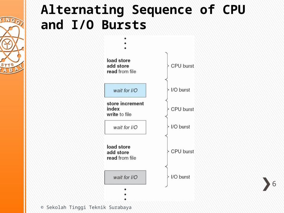
Alternating Sequence of CPU and I/O Bursts
6
© Sekolah Tinggi Teknik Surabaya
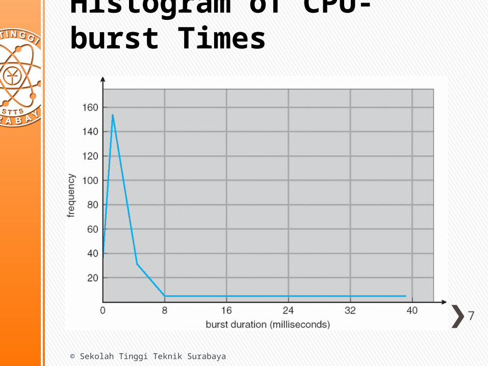
Histogram of CPU-burst Times
7
© Sekolah Tinggi Teknik Surabaya
CPU Scheduler» Selects from among the processes in ready queue,
and allocates the CPU to one of them˃ Queue may be ordered in various ways
» CPU scheduling decisions may take place when a process:
1. Switches from running to waiting state2. Switches from running to ready state3. Switches from waiting to ready4. Terminates
» Scheduling under 1 and 4 is nonpreemptive» All other scheduling is preemptive
˃ Consider access to shared data˃ Consider preemption while in kernel mode˃ Consider interrupts occurring during crucial OS activities
8
© Sekolah Tinggi Teknik Surabaya
Dispatcher» Dispatcher module gives control of the
CPU to the process selected by the short-term scheduler; this involves:˃ switching context˃ switching to user mode˃ jumping to the proper location in the user
program to restart that program» Dispatch latency – time it takes for the
dispatcher to stop one process and start another running 9
© Sekolah Tinggi Teknik Surabaya
Scheduling Criteria© Sekolah Tinggi Teknik Surabaya
10
Scheduling Criteria» CPU utilization – keep the CPU as busy as
possible» Throughput – # of processes that complete
their execution per time unit» Turnaround time – amount of time to execute
a particular process» Waiting time – amount of time a process has
been waiting in the ready queue» Response time – amount of time it takes from
when a request was submitted until the first response is produced, not output (for time-sharing environment)
11
© Sekolah Tinggi Teknik Surabaya
Scheduling Algorithm© Sekolah Tinggi Teknik Surabaya
12
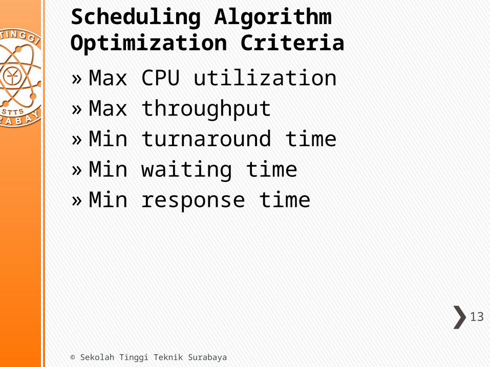
Scheduling Algorithm Optimization Criteria
» Max CPU utilization» Max throughput» Min turnaround time » Min waiting time » Min response time
13
© Sekolah Tinggi Teknik Surabaya

First-Come, First-Served (FCFS) Scheduling
Process Burst TimeP1 24 P2 3 P3 3
» Suppose that the processes arrive in the order: P1 , P2 , P3
The Gantt Chart for the schedule is:
» Waiting time for P1 = 0; P2 = 24; P3 = 27» Average waiting time: (0 + 24 + 27)/3 = 17
14
© Sekolah Tinggi Teknik Surabaya
P1 P2 P3
24 27 300
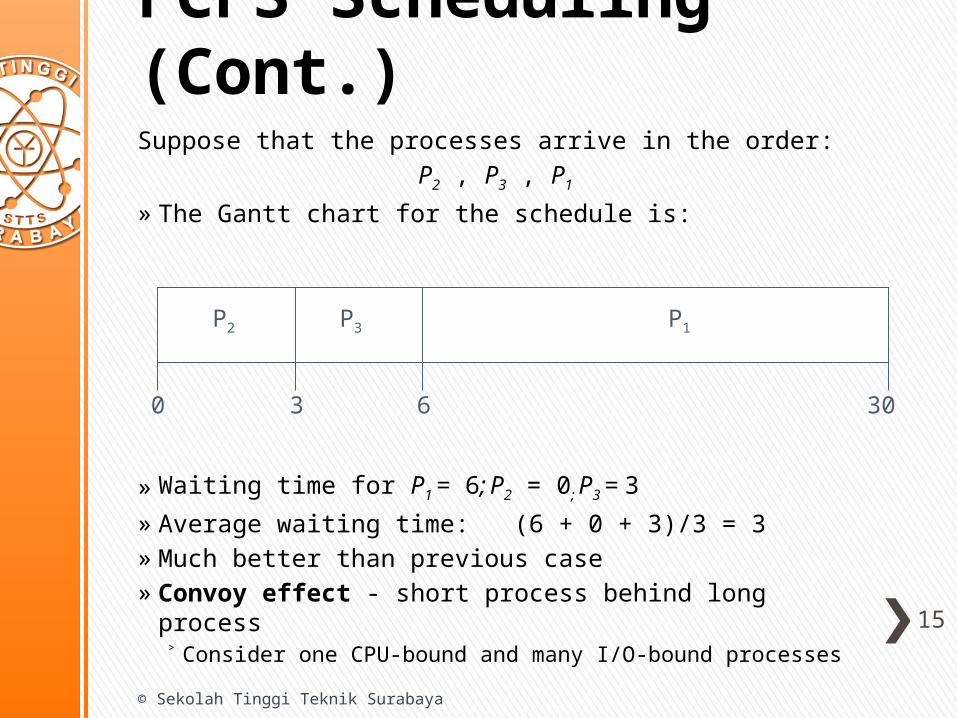
FCFS Scheduling (Cont.)Suppose that the processes arrive in the order:
P2 , P3 , P1 » The Gantt chart for the schedule is:
» Waiting time for P1 = 6; P2 = 0; P3 = 3» Average waiting time: (6 + 0 + 3)/3 = 3» Much better than previous case» Convoy effect - short process behind long process
˃ Consider one CPU-bound and many I/O-bound processes
15
© Sekolah Tinggi Teknik Surabaya
P1P3P2
63 300
Shortest-Job-First (SJF) Scheduling» Associate with each process the length
of its next CPU burst˃ Use these lengths to schedule the process
with the shortest time» SJF is optimal – gives minimum average
waiting time for a given set of processes˃ The difficulty is knowing the length of the
next CPU request˃ Could ask the user
16
© Sekolah Tinggi Teknik Surabaya
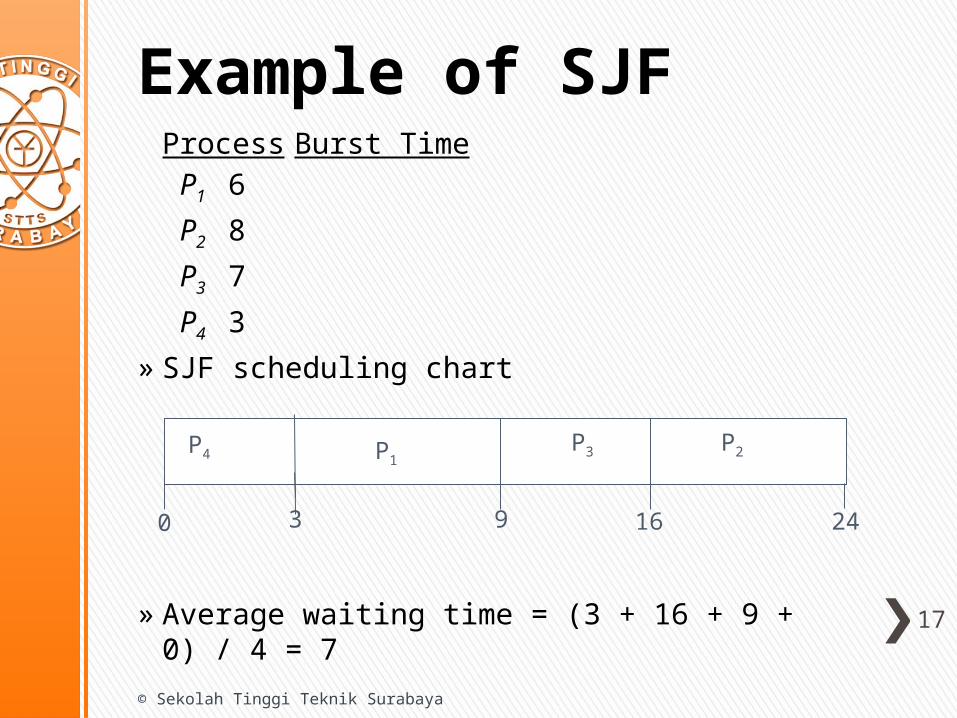
Example of SJFProcess Burst Time P1 6
P2 8
P3 7
P4 3» SJF scheduling chart
» Average waiting time = (3 + 16 + 9 + 0) / 4 = 7
17
© Sekolah Tinggi Teknik Surabaya
P4P3P1
3 160 9
P2
24
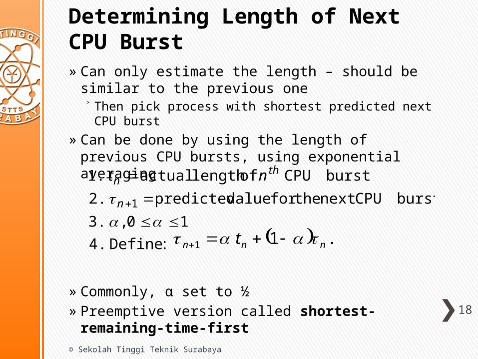
Determining Length of Next CPU Burst» Can only estimate the length – should be similar to
the previous one˃ Then pick process with shortest predicted next CPU burst
» Can be done by using the length of previous CPU bursts, using exponential averaging
» Commonly, α set to ½» Preemptive version called shortest-remaining-time-
first18
© Sekolah Tinggi Teknik Surabaya
:Define 4.
10 , 3.
burst CPU next the for value predicted 2.
burst CPU of length actual 1.
1n
thn nt
.1 1 nnn t
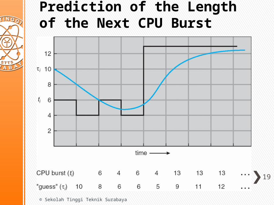
Prediction of the Length of the Next CPU Burst
19
© Sekolah Tinggi Teknik Surabaya
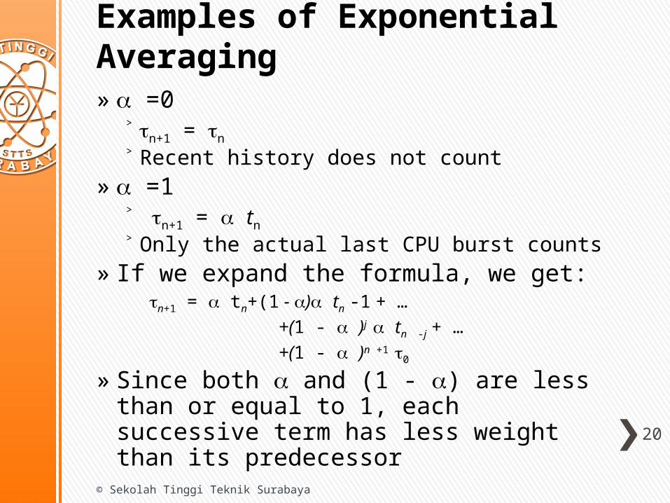
Examples of Exponential Averaging» =0
˃ n+1 = n
˃ Recent history does not count» =1
˃ n+1 = tn
˃ Only the actual last CPU burst counts» If we expand the formula, we get:
n+1 = tn+(1 - ) tn -1 + … +(1 - )j tn -j + … +(1 - )n +1 0
» Since both and (1 - ) are less than or equal to 1, each successive term has less weight than its predecessor
20
© Sekolah Tinggi Teknik Surabaya
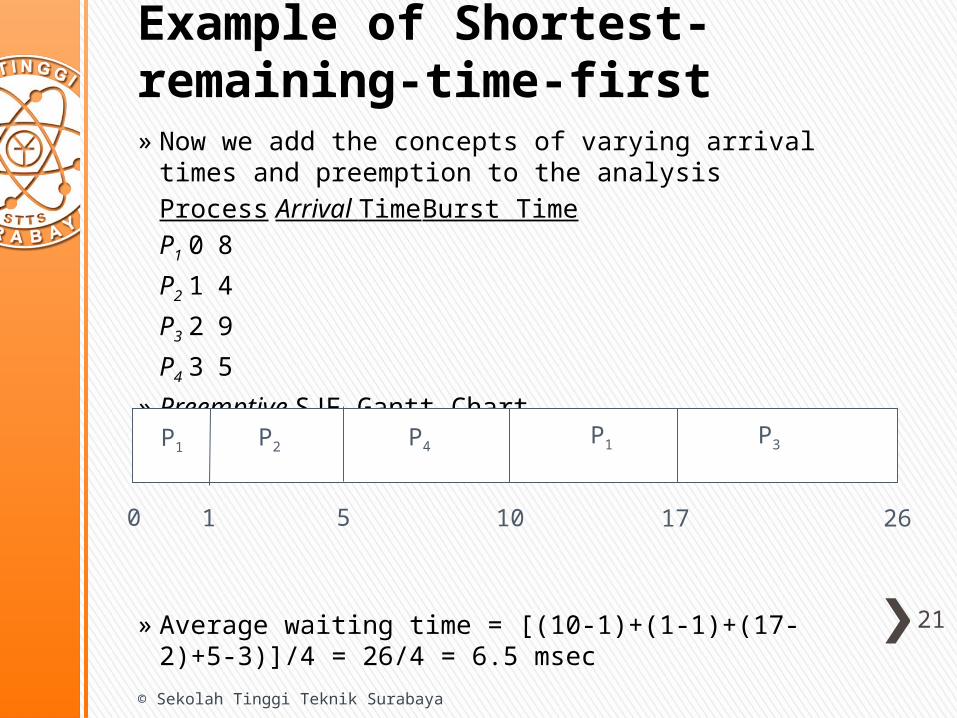
Example of Shortest-remaining-time-first» Now we add the concepts of varying arrival times and
preemption to the analysisProcess Arrival Time Burst TimeP1 0 8
P2 1 4
P3 2 9
P4 3 5» Preemptive SJF Gantt Chart
» Average waiting time = [(10-1)+(1-1)+(17-2)+5-3)]/4 = 26/4 = 6.5 msec
21
© Sekolah Tinggi Teknik Surabaya
P1P1P2
1 170 10
P3
265
P4
Priority Scheduling» A priority number (integer) is associated with
each process» The CPU is allocated to the process with the
highest priority (smallest integer highest priority)˃ Preemptive˃ Nonpreemptive
» SJF is priority scheduling where priority is the inverse of predicted next CPU burst time
» Problem Starvation – low priority processes may never execute
» Solution Aging – as time progresses increase the priority of the process
22
© Sekolah Tinggi Teknik Surabaya
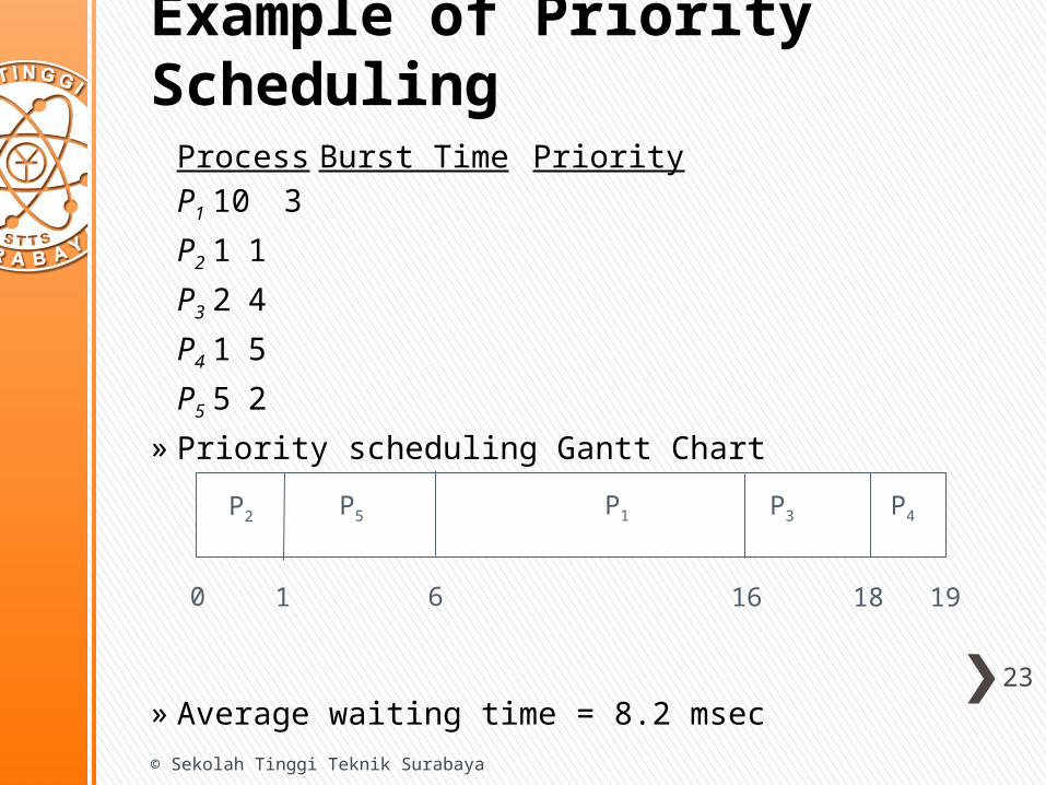
Example of Priority SchedulingProcess Burst Time PriorityP1 10 3
P2 1 1
P3 2 4
P4 1 5
P5 5 2» Priority scheduling Gantt Chart
» Average waiting time = 8.2 msec
23
© Sekolah Tinggi Teknik Surabaya
P2 P3P5
1 180 16
P4
196
P1
Round Robin (RR)» Each process gets a small unit of CPU time (time
quantum q), usually 10-100 milliseconds. After this time has elapsed, the process is preempted and added to the end of the ready queue.
» If there are n processes in the ready queue and the time quantum is q, then each process gets 1/n of the CPU time in chunks of at most q time units at once. No process waits more than (n-1)q time units.
» Timer interrupts every quantum to schedule next process
» Performance˃ q large FIFO˃ q small q must be large with respect to context switch,
otherwise overhead is too high
24
© Sekolah Tinggi Teknik Surabaya
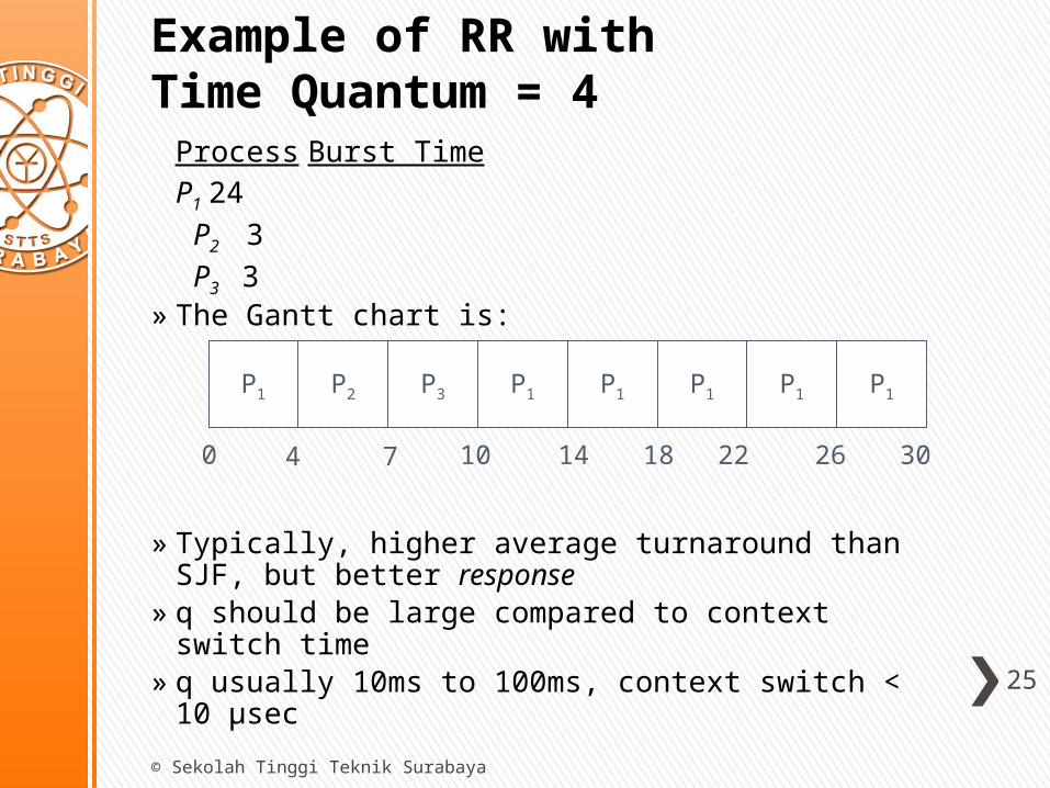
Example of RR withTime Quantum = 4
Process Burst TimeP1 24 P2 3 P3 3
» The Gantt chart is:
» Typically, higher average turnaround than SJF, but better response
» q should be large compared to context switch time» q usually 10ms to 100ms, context switch < 10 μsec
25
© Sekolah Tinggi Teknik Surabaya
P1 P2 P3 P1 P1 P1 P1 P1
0 4 7 10 14 18 22 26 30
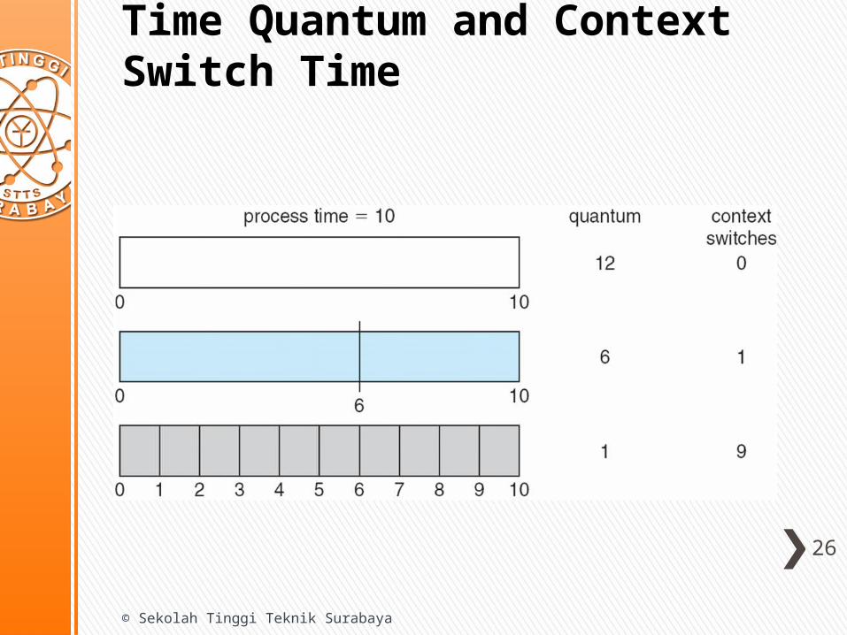
Time Quantum and Context Switch Time
26
© Sekolah Tinggi Teknik Surabaya

Turnaround Time Varies With The Time Quantum
27
© Sekolah Tinggi Teknik Surabaya
80% of CPU bursts should be shorter than q

Multilevel Queue» Ready queue is partitioned into separate queues, e.g.:
˃ foreground (interactive)˃ background (batch)
» Process permanently in a given queue» Each queue has its own scheduling algorithm:
˃ foreground – RR˃ background – FCFS
» Scheduling must be done between the queues:˃ Fixed priority scheduling; (i.e., serve all from foreground
then from background). Possibility of starvation.˃ Time slice – each queue gets a certain amount of CPU
time which it can schedule amongst its processes; i.e., 80% to foreground in RR
˃ 20% to background in FCFS 28
© Sekolah Tinggi Teknik Surabaya
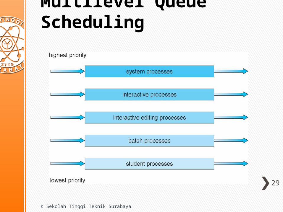
Multilevel Queue Scheduling
29
© Sekolah Tinggi Teknik Surabaya
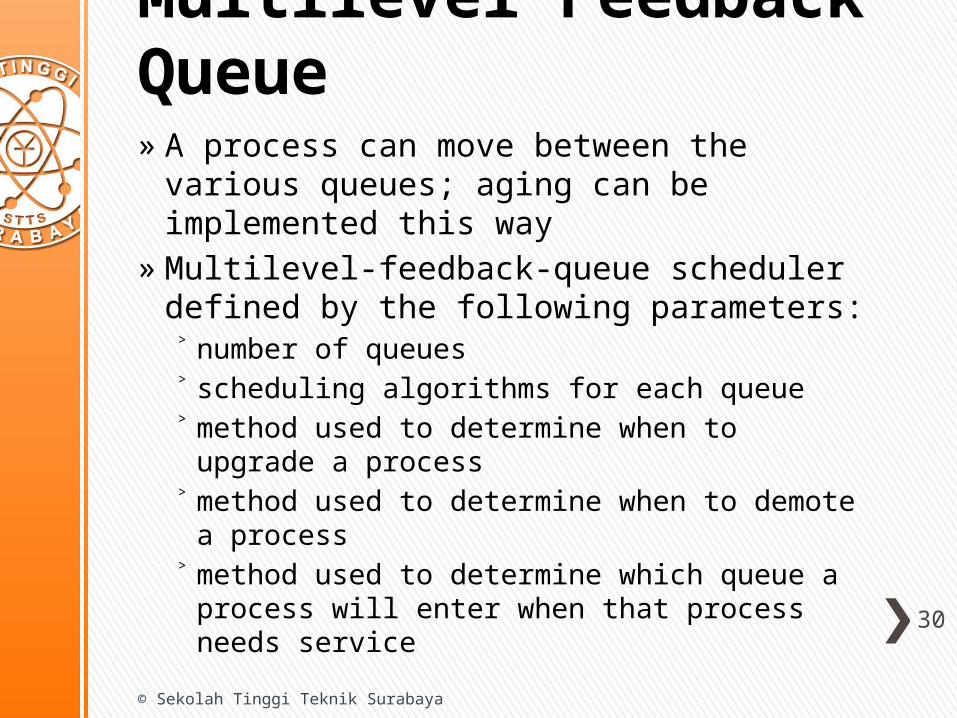
Multilevel Feedback Queue» A process can move between the various
queues; aging can be implemented this way» Multilevel-feedback-queue scheduler defined
by the following parameters:˃ number of queues˃ scheduling algorithms for each queue˃ method used to determine when to upgrade a
process˃ method used to determine when to demote a
process˃ method used to determine which queue a process
will enter when that process needs service 30
© Sekolah Tinggi Teknik Surabaya
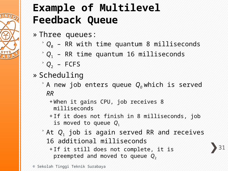
Example of Multilevel Feedback Queue» Three queues:
˃ Q0 – RR with time quantum 8 milliseconds
˃ Q1 – RR time quantum 16 milliseconds
˃ Q2 – FCFS
» Scheduling˃ A new job enters queue Q0 which is served RR
+ When it gains CPU, job receives 8 milliseconds+ If it does not finish in 8 milliseconds, job is moved to
queue Q1
˃ At Q1 job is again served RR and receives 16 additional milliseconds
+ If it still does not complete, it is preempted and moved to queue Q2
31
© Sekolah Tinggi Teknik Surabaya
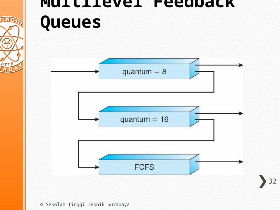
Multilevel Feedback Queues
32
© Sekolah Tinggi Teknik Surabaya
© Sekolah Tinggi Teknik Surabaya
33Thread Scheduling
Thread Scheduling» Distinction between user-level and kernel-level
threads» When threads supported, threads scheduled, not
processes» Many-to-one and many-to-many models, thread
library schedules user-level threads to run on LWP˃ Known as process-contention scope (PCS) since
scheduling competition is within the process˃ Typically done via priority set by programmer
» Kernel thread scheduled onto available CPU is system-contention scope (SCS) – competition among all threads in system
34
© Sekolah Tinggi Teknik Surabaya
Multiple Processor Scheduling© Sekolah Tinggi Teknik Surabaya
35
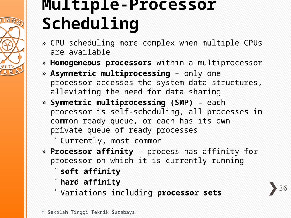
Multiple-Processor Scheduling» CPU scheduling more complex when multiple CPUs are
available» Homogeneous processors within a multiprocessor» Asymmetric multiprocessing – only one processor
accesses the system data structures, alleviating the need for data sharing
» Symmetric multiprocessing (SMP) – each processor is self-scheduling, all processes in common ready queue, or each has its own private queue of ready processes˃ Currently, most common
» Processor affinity – process has affinity for processor on which it is currently running˃ soft affinity˃ hard affinity˃ Variations including processor sets
36
© Sekolah Tinggi Teknik Surabaya
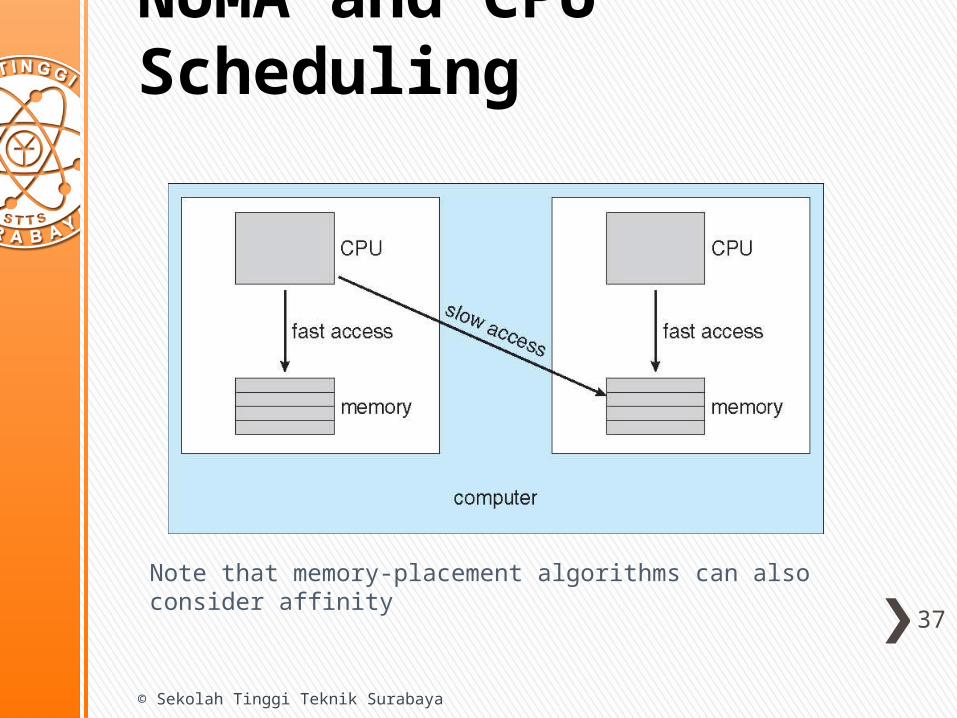
NUMA and CPU Scheduling
37
© Sekolah Tinggi Teknik Surabaya
Note that memory-placement algorithms can also consider affinity
Multicore Processors» Recent trend to place multiple
processor cores on same physical chip» Faster and consumes less power» Multiple threads per core also growing
˃ Takes advantage of memory stall to make progress on another thread while memory retrieve happens
38
© Sekolah Tinggi Teknik Surabaya
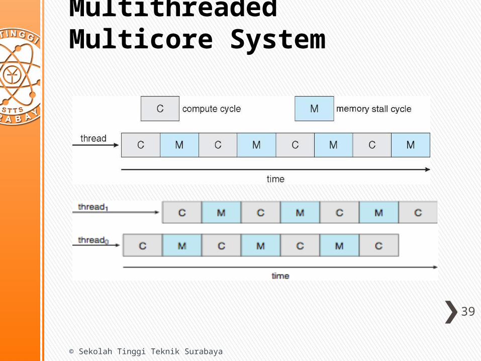
Multithreaded Multicore System
39
© Sekolah Tinggi Teknik Surabaya
Virtualization and Scheduling» Virtualization software schedules
multiple guests onto CPU(s)» Each guest doing its own scheduling
˃ Not knowing it doesn’t own the CPUs˃ Can result in poor response time˃ Can effect time-of-day clocks in guests
» Can undo good scheduling algorithm efforts of guests
40
© Sekolah Tinggi Teknik Surabaya
Algorithm Evaluation© Sekolah Tinggi Teknik Surabaya
41
Algorithm Evaluation» How to select CPU-scheduling algorithm
for an OS?» Determine criteria, then evaluate
algorithms
42
© Sekolah Tinggi Teknik Surabaya
Deterministic Modeling» Type of analytic evaluation» Takes a particular predetermined
workload and defines the performance of each algorithm for that workload
43
© Sekolah Tinggi Teknik Surabaya
Queueing Models» Describes the arrival of processes, and CPU
and I/O bursts probabilistically˃ Commonly exponential, and described by
mean˃ Computes average throughput, utilization,
waiting time, etc» Computer system described as network of
servers, each with queue of waiting processes˃ Knowing arrival rates and service rates˃ Computes utilization, average queue length,
average wait time, etc44
© Sekolah Tinggi Teknik Surabaya
Little’s Formula» n = average queue length» W = average waiting time in queue» λ = average arrival rate into queue» Little’s law – in steady state, processes leaving
queue must equal processes arriving, thusn = λ x W˃ Valid for any scheduling algorithm and arrival
distribution» For example, if on average 7 processes arrive
per second, and normally 14 processes in queue, then average wait time per process = 2 seconds
45
© Sekolah Tinggi Teknik Surabaya
Simulations» Queueing models limited» Simulations more accurate
˃ Programmed model of computer system˃ Clock is a variable˃ Gather statistics indicating algorithm
performance˃ Data to drive simulation gathered via
+ Random number generator according to probabilities
+ Distributions defined mathematically or empirically+ Trace tapes record sequences of real events in real
systems 46
© Sekolah Tinggi Teknik Surabaya

Simulations
47
© Sekolah Tinggi Teknik Surabaya
End ofLecture 4© Sekolah Tinggi Teknik Surabaya
48
Recommended