Lecture 9:Advanced DFT concepts: The
Exchange-correlation functional and time-dependent DFT
Marie Curie Tutorial Series: Modeling BiomoleculesDecember 6-11, 2004
Mark TuckermanDept. of Chemistry
and Courant Institute of Mathematical Science100 Washington Square East
New York University, New York, NY 10003
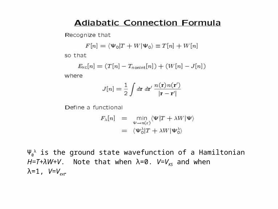
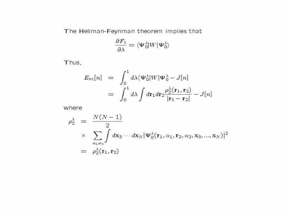
Ψ0λ is the ground state wavefunction of a Hamiltonian
H=T+λW+V. Note that when λ=0. V=VKS and when λ=1, V=Vext.
λ λ
λ λ
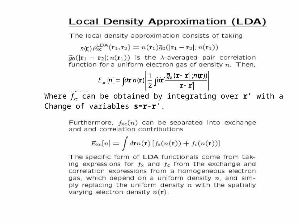
0 ( ; ( ))1[ ] ( )
2xc
g nE n d n d
r r r
r r rr r
1( )n r
Where fxc can be obtained by integrating over r’ with aChange of variables s=r-r’.
2
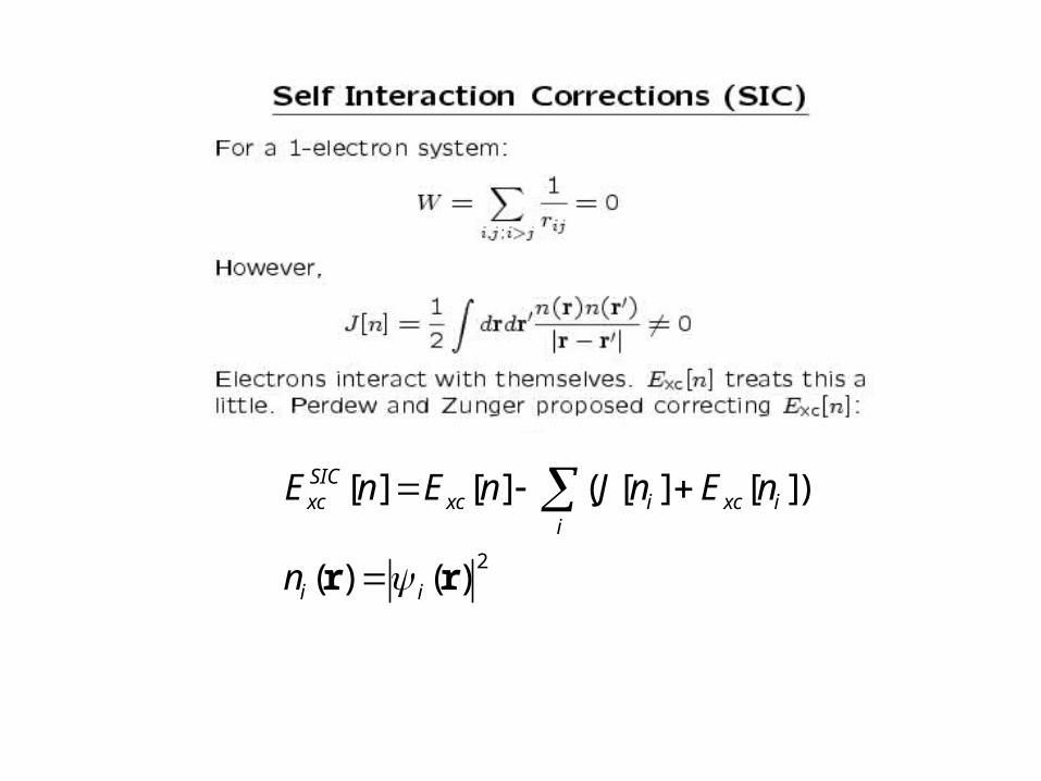
[ ] [ ] ( [ ] [ ])
( ) ( )
SICxc xc i xc i
i
i i
E n E n J n E n
n
r r
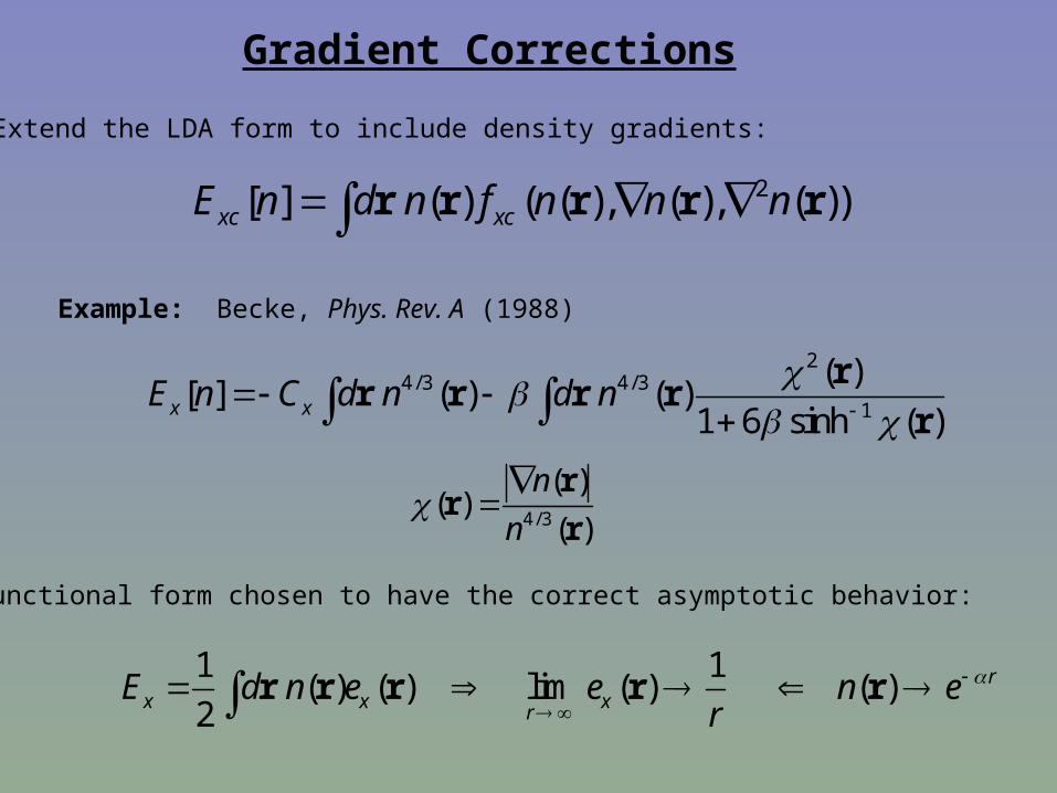
Gradient Corrections
Extend the LDA form to include density gradients:
2[ ] ( ) ( ( ), ( ), ( ))xc xcE n d n f n n n r r r r r
Example: Becke, Phys. Rev. A (1988)
24/3 4 /3
1
( )[ ] ( ) ( )
1 6 sinh ( )x xE n C d n d n
rr r r r
r
4/3
( )( )
( )
n
n
rr
r
Functional form chosen to have the correct asymptotic behavior:
1 1 ( ) ( ) lim ( ) ( )
2r
x x xrE d n e e n e
r
r r r r r
Motivation for TDDFT
• Photoexcitation processes• Atomic and nuclear scattering• Dynamical response of inhomogeneous metallic systems.
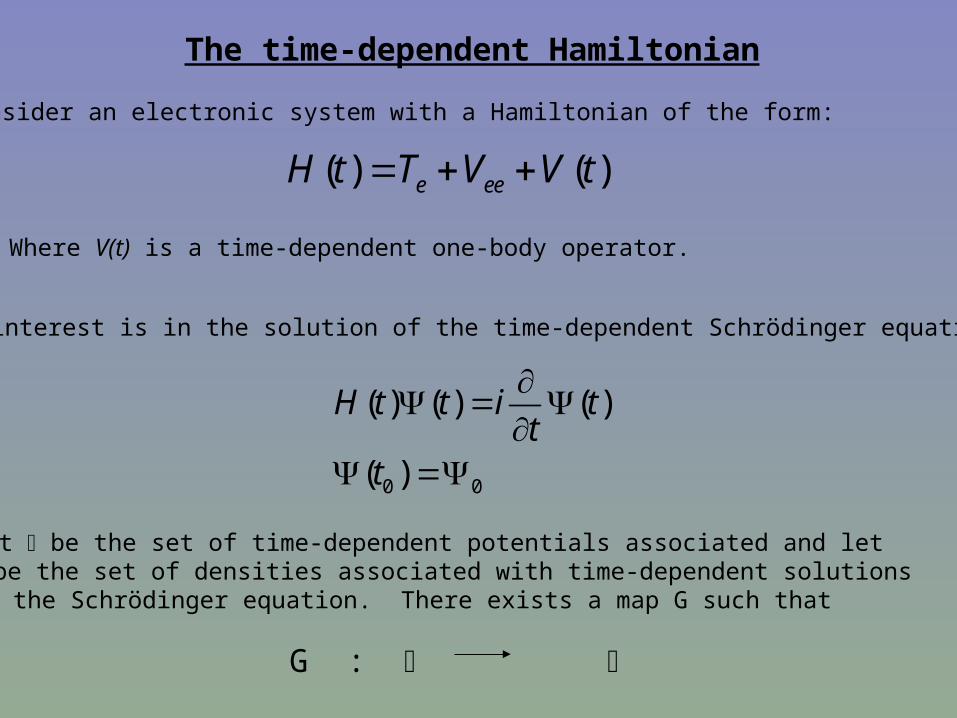
The time-dependent Hamiltonian
Consider an electronic system with a Hamiltonian of the form:
( ) ( )e eeH t T V V t
Where V(t) is a time-dependent one-body operator.
Our interest is in the solution of the time-dependent Schrödinger equation:
0 0
( ) ( ) ( )
( )
H t t i tt
t
Let be the set of time-dependent potentials associated and let be the set of densities associated with time-dependent solutionsof the Schrödinger equation. There exists a map G such that
G :
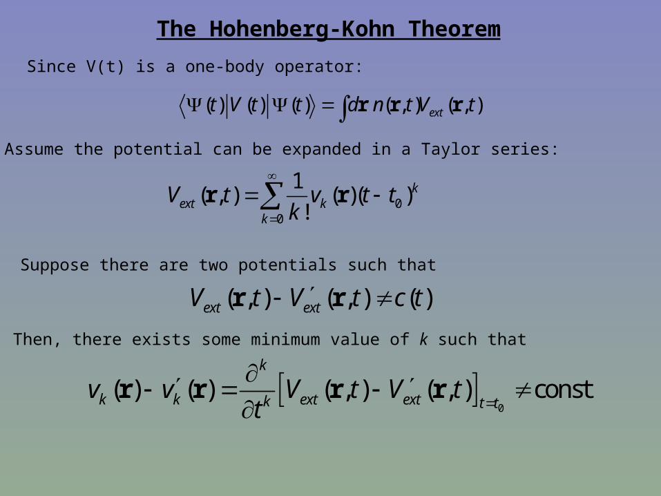
The Hohenberg-Kohn Theorem
Since V(t) is a one-body operator:
( ) ( ) ( ) ( , ) ( , )extt V t t d n t V t r r r
Assume the potential can be expanded in a Taylor series:
00
1( , ) ( )( )
!k
ext kk
V t v t tk
r r
Suppose there are two potentials such that
( , ) ( , ) ( )ext extV t V t c t r r
Then, there exists some minimum value of k such that
0
( ) ( ) ( , ) ( , ) constk
k k ext extk t tv v V t V t
t
r r r r
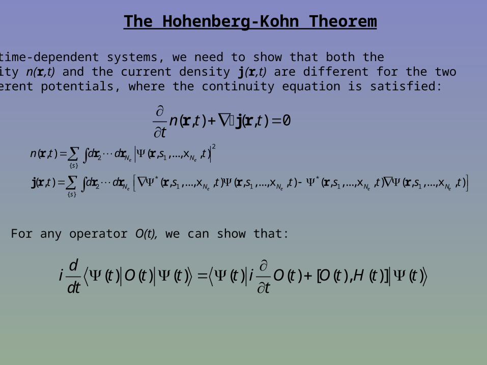
The Hohenberg-Kohn Theorem
For time-dependent systems, we need to show that both thedensity n(r,t) and the current density j(r,t) are different for the twodifferent potentials, where the continuity equation is satisfied:
( , ) ( , ) 0n t tt
r j r
For any operator O(t), we can show that:
( ) ( ) ( ) ( ) ( ) [ ( ), ( )] ( )d
i t O t t t i O t O t H t tdt t
2
2 1{ }
* *2 1 1 1 1
{ }
( , ) ( , ,..., x , )
( , ) ( , ,..., x , ) ( , ,..., x , ) ( , ,..., x , ) ( , ,..., x , )
e e
e e e e e
N Ns
N N N N Ns
n t d d s t
t d d s t s t s t s t
r r r r
j r r r r r r r
The Hohenberg-Kohn Theorem
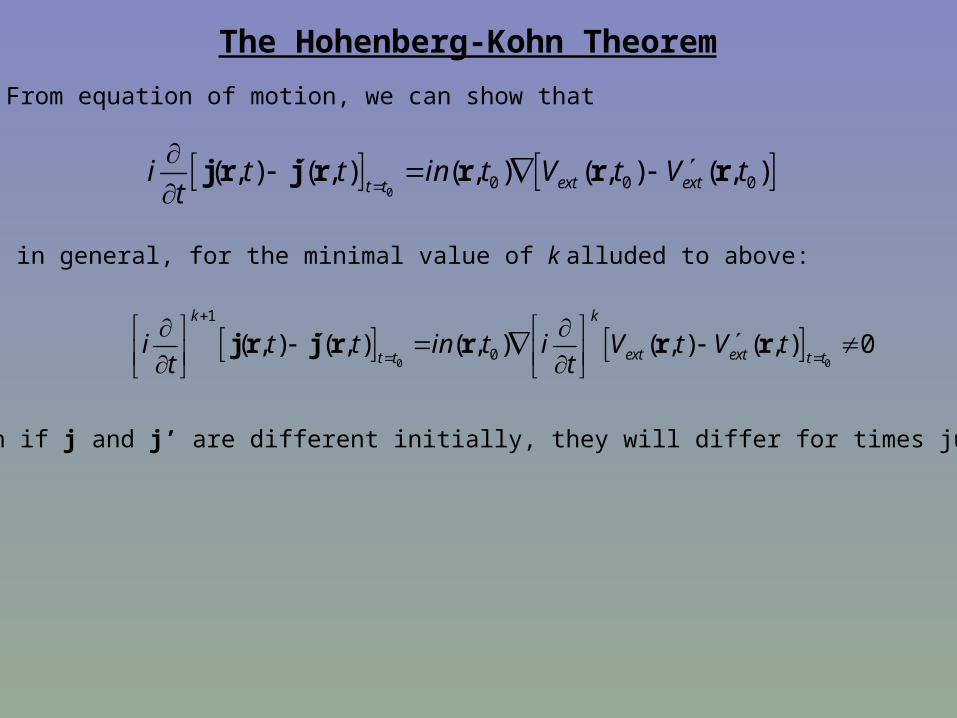
From equation of motion, we can show that
0
0 0 0( , ) ( , ) ( , ) ( , ) ( , )ext extt ti t t in t V t V t
t
j r j r r r r
And, in general, for the minimal value of k alluded to above:
0 0
1
0( , ) ( , ) ( , ) ( , ) ( , ) 0k k
ext extt t t ti t t in t i V t V t
t t
j r j r r r r
Hence, even if j and j’ are different initially, they will differ for times just laterthan t0.
The Hohenberg-Kohn Theorem
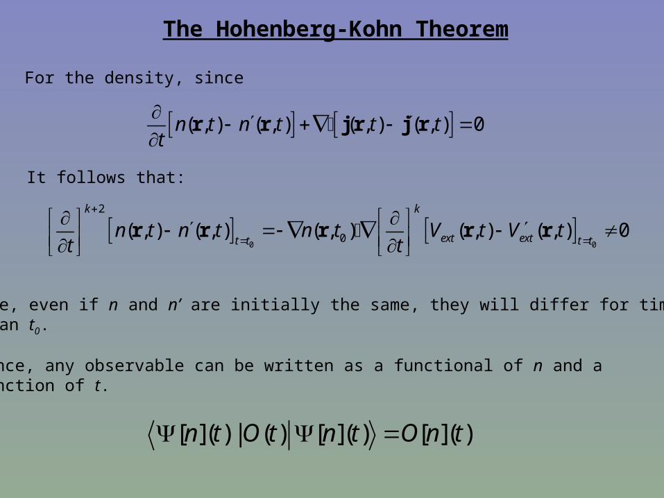
For the density, since
( , ) ( , ) ( , ) ( , ) 0n t n t t tt
r r j r j r
0 0
2
0( , ) ( , ) ( , ) ( , ) ( , ) 0k k
ext extt t t tn t n t n t V t V t
t t
r r r r r
It follows that:
Therefore, even if n and n’ are initially the same, they will differ for times justlater than t0.
[ ]( ) | ( ) [ ]( ) [ ]( )n t O t n t O n t
Hence, any observable can be written as a functional of n and afunction of t.
Actions in quantum mechanics and DFT
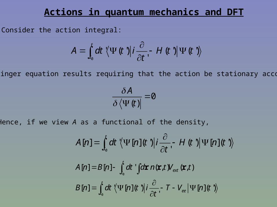
Consider the action integral:
0
' ( ') ( ') ( ')'
t
tA dt t i H t t
t
Schrödinger equation results requiring that the action be stationary according to:
0( )
A
t
Hence, if we view A as a functional of the density,
0
[ ] ' [ ]( ') ( ') [ ]( ')'
t
tA n dt n t i H t n t
t
0
0
[ ] [ ] ' ( , ) ( , )
[ ] ' [ ]( ') [ ]( ')'
t
extt
t
eet
A n B n dt d n t V t
B n dt n t i T V n tt
r r r
Hohenberg-Kohn and KS schemes
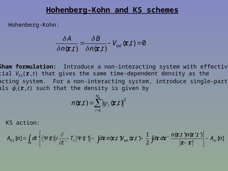
Hohenberg-Kohn:
( , ) 0( , ) ( , ) ext
A BV t
n t n t
rr r
Kohn-Sham formulation: Introduce a non-interacting system with effectivepotential VKS(r,t) that gives the same time-dependent density as theinteracting system. For a non-interacting system, introduce single-particleorbitals ψi(r,t) such that the density is given by
2
1
( , ) ( , )eN
ii
n t t
r r
KS action:
0
1 ( , ') ( ', ')[ ] ' ( ) ( ') ( , ') ( , ') ' [ ]
' 2 '
t
KS s ext xct
n t n tA n dt t i T t d n t V t d d A n
t
r rr r r r r
r r
21( , ) ( , ) ( , )
2
( ', )( , ) ( , ) '
' ( , )
i KS i
xcKS ext
i t V t tt
An tV t V t d
n t
r r r
rr r r
r r r
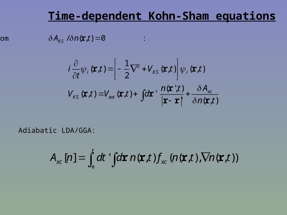
Time-dependent Kohn-Sham equations
From :/ ( , ) 0KSA n t r
Adiabatic LDA/GGA:
0
[ ] ' ( , ) ( ( , ), ( , ))t
xc xctA n dt d n t f n t n t r r r r
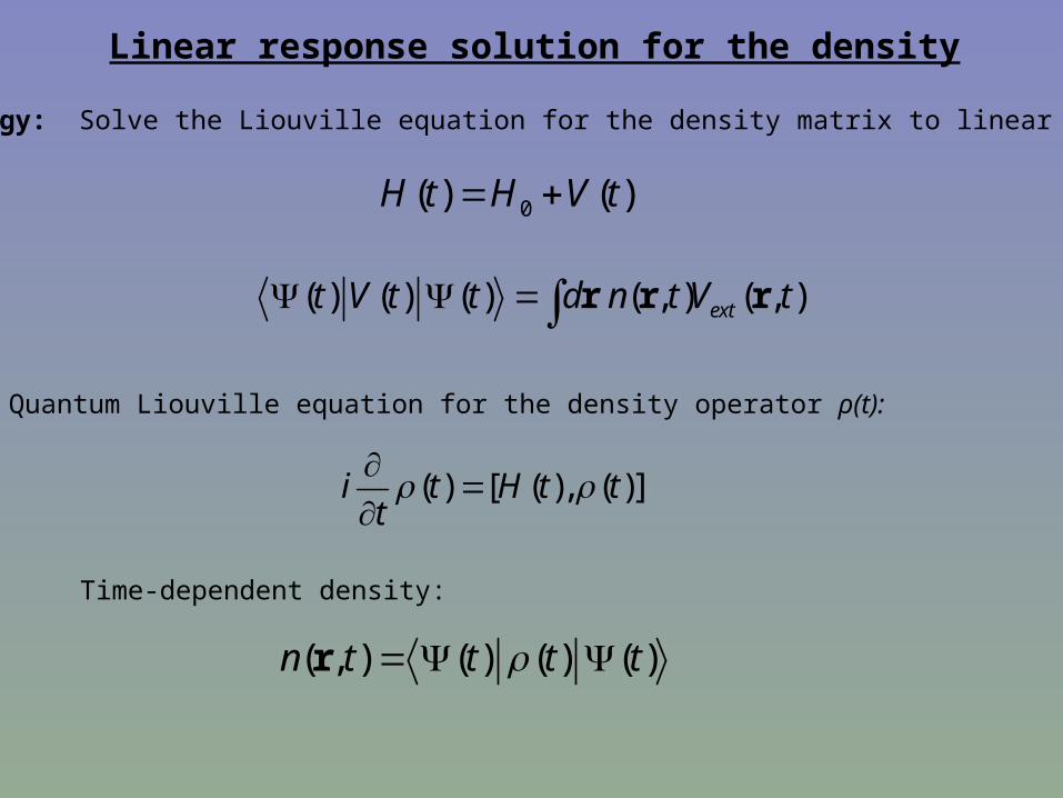
Linear response solution for the density
Strategy: Solve the Liouville equation for the density matrix to linear order.
0( ) ( )H t H V t
Quantum Liouville equation for the density operator ρ(t):
( ) [ ( ), ( )]i t H t tt
Time-dependent density:
( , ) ( ) ( ) ( )n t t t t r
( ) ( ) ( ) ( , ) ( , )extt V t t d n t V t r r r
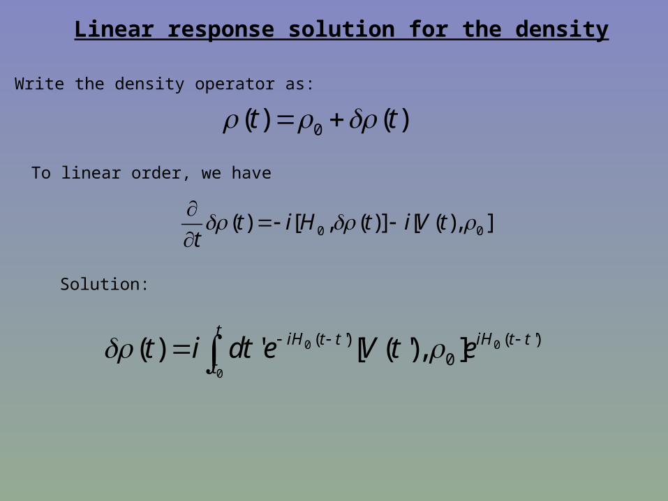
Linear response solution for the density
Write the density operator as:
0( ) ( )t t
To linear order, we have
0 0( ) [ , ( )] [ ( ), ]t i H t i V tt
Solution:
0 0
0
( ') ( ')0( ) ' [ ( '), ]
t iH t t iH t t
tt i dt e V t e
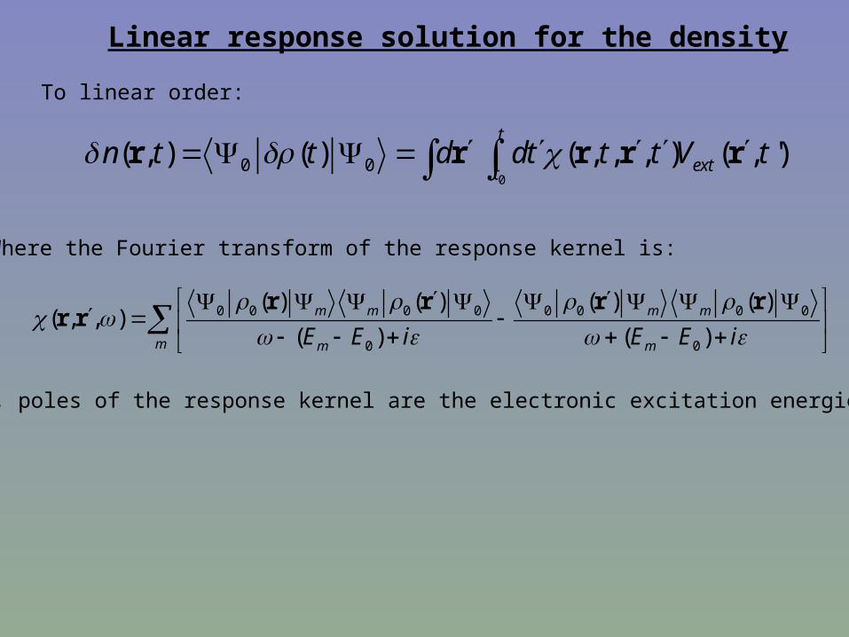
Linear response solution for the density
To linear order:
00 0( , ) ( ) ( , , , ) ( , ')
t
exttn t t d dt t t V t r r r r r
Where the Fourier transform of the response kernel is:
0 0 0 0 0 0 0 0
0 0
( ) ( ) ( ) ( )( , , )
( ) ( )m m m m
m m mE E i E E i
r r r rr r
Hence, poles of the response kernel are the electronic excitation energies.
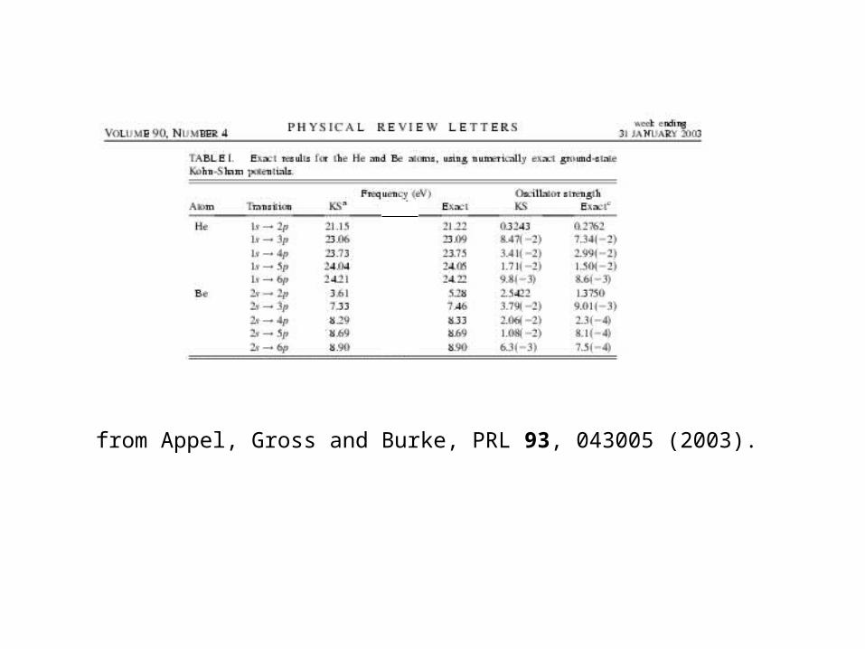
from Appel, Gross and Burke, PRL 93, 043005 (2003).
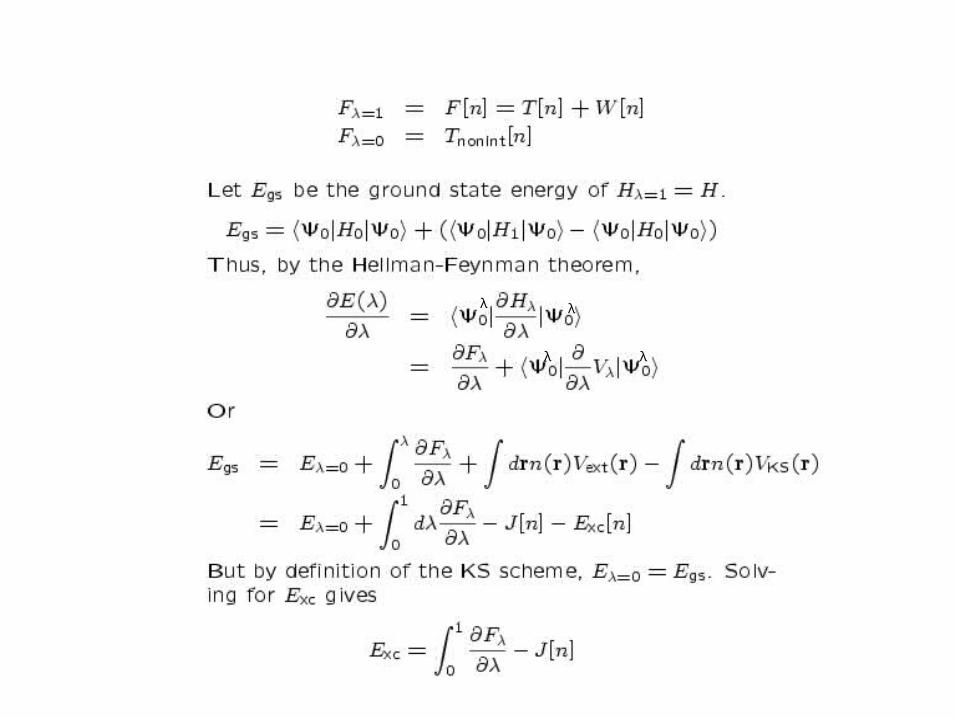
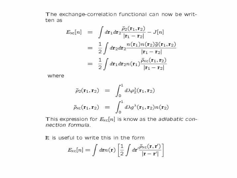
Lecture Summary• Adiabatic connection formula provides a rigorous theory of the
exchange-correlation functional and is the starting point of many approximations.
• Generalization of density functional theory to time-dependent systems is possible through generalization of the Hohenberg-Kohn theorem.
• In linear response theory, the response kernel (or its poles) is the object of interest as it yields the excitation energies.
Recommended