Measuring and Predicting Liquidity
in the
Stock Market
DISSERTATION
der Universitat St. Gallen,
Hochschule fur Wirtschafts-,
Rechts- und Sozialwissenschaften (HSG)
zur Erlangung der Wurde eines
Doktors der Wirtschaftswissenschaften
vorgelegt von
Rico von Wyssvon
Zurich
Genehmigt auf Antrag der Herren
Prof. Dr. Heinz Zimmermann
und
Prof. Dr. Alex Keel
Dissertation Nr. 2899
Novidea di Luigi Hofmann, Riazzino 2004

Die Universitat St. Gallen, Hochschule fur Wirtschafts-, Rechts- und Sozialwissenschaften
(HSG), gestattet hiermit die Drucklegung der vorliegenden Dissertation, ohne damit zu den
darin ausgesprochenen Anschauungen Stellung zu nehmen.
St. Gallen, den 13. Januar 2004
Der Rektor:
Prof. Dr. Peter Gomez

To Anna


Acknowledgements
During the last three years, I spent a marvellous time as teaching and research assistant
at the Swiss Institute of Banking and Finance of the University of St. Gallen. Each of my
superiors Heinz Zimmermann, Andreas Grunbichler and Manuel Ammann provided me with
valuable insights in the academic life and stimulated my research interests. My thanks are
also due to my colleagues at the institute who encouraged me during my thesis project. I
shared many fruitful discussions with them.
I am very indebted to my academic advisor Heinz Zimmermann and my co-advisor Alex
Keel for their ongoing support and their helpful hints which made this thesis possible.
My thanks go also to Charlie Beckwith for carefully proof-reading my English. I ac-
knowledge financial support from the Forderervereinigung des Schweizerischen Institutes fur
Banken und Finanzen der Universitat St. Gallen.
My parents supported me wherever possible during my whole life and enabled me to
pursue my education. They deserve my sincere gratitude.
Finally, my thanks go to my wife Nadja Germann who finishes her thesis just at the same
time. Her parents had to bear our frequent absences from home and took great care of our
daughter Anna.
St. Gallen, January 2004
Rico von Wyss
v

Contents
List of Figures xi
List of Tables xiii
Introduction xvii
I Liquidity – Definition and Measurement 1
1 Liquidity in an Economic Framework 5
1.1 Properties of Liquidity . . . . . . . . . . . . . . . . . . . . . . . . . . . . . . 5
1.2 Liquidity Measures . . . . . . . . . . . . . . . . . . . . . . . . . . . . . . . . 9
1.2.1 One-dimensional Liquidity Measures . . . . . . . . . . . . . . . . . . 9
1.2.2 Multi-dimensional Liquidity Measures . . . . . . . . . . . . . . . . . . 16
2 Data and Institutional Setting 23
2.1 The Limit Order Book of the Swiss Exchange . . . . . . . . . . . . . . . . . 23
2.2 Data . . . . . . . . . . . . . . . . . . . . . . . . . . . . . . . . . . . . . . . . 27
3 Summary Statistics and Correlations 31
3.1 Summary Statistics of the Liquidity Measures . . . . . . . . . . . . . . . . . 32
3.1.1 Summary Statistics of Adecco . . . . . . . . . . . . . . . . . . . . . . 32
3.1.2 Summary Statistics of Baer . . . . . . . . . . . . . . . . . . . . . . . 33
3.1.3 Summary Statistics of Richemont . . . . . . . . . . . . . . . . . . . . 35
3.1.4 Summary Statistics of Ciba . . . . . . . . . . . . . . . . . . . . . . . 36
3.1.5 Summary Statistics of Clariant . . . . . . . . . . . . . . . . . . . . . 37
3.1.6 Summary Statistics of Givaudan . . . . . . . . . . . . . . . . . . . . . 38
3.1.7 Summary Statistics of Holcim . . . . . . . . . . . . . . . . . . . . . . 40
3.1.8 Summary Statistics of Kudelski . . . . . . . . . . . . . . . . . . . . . 41
3.1.9 Summary Statistics of Lonza . . . . . . . . . . . . . . . . . . . . . . . 42
3.1.10 Summary Statistics of Swiss Re . . . . . . . . . . . . . . . . . . . . . 43
3.1.11 Summary Statistics of Swisscom . . . . . . . . . . . . . . . . . . . . . 44
3.1.12 Summary Statistics of Serono . . . . . . . . . . . . . . . . . . . . . . 45
3.1.13 Summary Statistics of Surveillance . . . . . . . . . . . . . . . . . . . 46
3.1.14 Summary Statistics of Sulzer . . . . . . . . . . . . . . . . . . . . . . . 48
3.1.15 Summary Statistics of Syngenta . . . . . . . . . . . . . . . . . . . . . 49
3.1.16 Summary Statistics of Swatch Bearer Share . . . . . . . . . . . . . . 50
vii
viii CONTENTS
3.1.17 Summary Statistics of Swatch Registered Share . . . . . . . . . . . . 50
3.1.18 Summary Statistics of Unaxis . . . . . . . . . . . . . . . . . . . . . . 52
3.1.19 General Remarks about the Summary Statistics . . . . . . . . . . . . 53
3.2 Stock Ranking according to Liquidity . . . . . . . . . . . . . . . . . . . . . . 54
3.3 Correlations of the Liquidity Measures . . . . . . . . . . . . . . . . . . . . . 57
4 Principal Component Analysis 59
4.1 Principal Component Analysis . . . . . . . . . . . . . . . . . . . . . . . . . . 59
4.2 Principal Component Analysis of Adecco . . . . . . . . . . . . . . . . . . . . 60
4.3 Principal Component Analysis of Baer . . . . . . . . . . . . . . . . . . . . . 62
4.4 Principal Component Analysis of Richemont . . . . . . . . . . . . . . . . . . 63
4.5 Principal Component Analysis of Ciba . . . . . . . . . . . . . . . . . . . . . 65
4.6 Principal Component Analysis of Clariant . . . . . . . . . . . . . . . . . . . 66
4.7 Principal Component Analysis of Givaudan . . . . . . . . . . . . . . . . . . . 68
4.8 Principal Component Analysis of Holcim . . . . . . . . . . . . . . . . . . . . 69
4.9 Principal Component Analysis of Kudelski . . . . . . . . . . . . . . . . . . . 71
4.10 Principal Component Analysis of Lonza . . . . . . . . . . . . . . . . . . . . . 72
4.11 Principal Component Analysis of Swiss Re . . . . . . . . . . . . . . . . . . . 74
4.12 Principal Component Analysis of Swisscom . . . . . . . . . . . . . . . . . . . 75
4.13 Principal Component Analysis of Serono . . . . . . . . . . . . . . . . . . . . 76
4.14 Principal Component Analysis of Surveillance . . . . . . . . . . . . . . . . . 77
4.15 Principal Component Analysis of Sulzer . . . . . . . . . . . . . . . . . . . . 79
4.16 Principal Component Analysis of Syngenta . . . . . . . . . . . . . . . . . . . 80
4.17 Principal Component Analysis of Swatch Bearer Share . . . . . . . . . . . . 82
4.18 Principal Component Analysis of Swatch Registered Share . . . . . . . . . . 83
4.19 Principal Component Analysis of Unaxis . . . . . . . . . . . . . . . . . . . . 83
4.20 General Results of the Principal Component Analysis . . . . . . . . . . . . . 85
II Predicting Liquidity 87
5 The Lead-Lag Behavior 91
5.1 Autocorrelation in Liquidity Measures and Returns . . . . . . . . . . . . . . 91
5.2 The Vector Autoregressive Model . . . . . . . . . . . . . . . . . . . . . . . . 92
5.3 Results of the VAR model for Adecco . . . . . . . . . . . . . . . . . . . . . . 93
5.4 Results of the VAR model for Baer . . . . . . . . . . . . . . . . . . . . . . . 96
5.5 Results of the VAR model for Richemont . . . . . . . . . . . . . . . . . . . . 98
5.6 Results of the VAR Model for Ciba . . . . . . . . . . . . . . . . . . . . . . . 101
5.7 Results of the VAR Model for Clariant . . . . . . . . . . . . . . . . . . . . . 103
5.8 Results of the VAR Model for Givaudan . . . . . . . . . . . . . . . . . . . . 105
5.9 Results of the VAR Model for Holcim . . . . . . . . . . . . . . . . . . . . . . 107
5.10 Results of the VAR Model for Kudelski . . . . . . . . . . . . . . . . . . . . . 110
5.11 Results of the VAR Model for Lonza . . . . . . . . . . . . . . . . . . . . . . 112
5.12 Results of the VAR Model for Swiss Re . . . . . . . . . . . . . . . . . . . . . 114
5.13 Results of the VAR Model for Swisscom . . . . . . . . . . . . . . . . . . . . 116
CONTENTS ix
5.14 Results of the VAR Model for Serono . . . . . . . . . . . . . . . . . . . . . . 118
5.15 Results of the VAR Model for Surveillance . . . . . . . . . . . . . . . . . . . 121
5.16 Results of the VAR Model for Sulzer . . . . . . . . . . . . . . . . . . . . . . 123
5.17 Results of the VAR Model for Syngenta . . . . . . . . . . . . . . . . . . . . . 125
5.18 Results of the VAR Model for Swatch Bearer Share . . . . . . . . . . . . . . 127
5.19 Results of the VAR Model for Swatch Registered Share . . . . . . . . . . . . 129
5.20 Results of the VAR Model for Unaxis . . . . . . . . . . . . . . . . . . . . . . 131
5.21 General Results of the VAR Model . . . . . . . . . . . . . . . . . . . . . . . 133
6 Prediction Models for Liquidity 137
6.1 Predicting the Relative Spread . . . . . . . . . . . . . . . . . . . . . . . . . . 137
6.2 Predicting Turnover . . . . . . . . . . . . . . . . . . . . . . . . . . . . . . . . 139
6.3 Predicting Dollar Depth . . . . . . . . . . . . . . . . . . . . . . . . . . . . . 139
6.4 Predicting Market Impact on the Ask-Side . . . . . . . . . . . . . . . . . . . 141
6.5 Predicting Market Impact on the Bid-Side . . . . . . . . . . . . . . . . . . . 143
6.6 Predicting the Liquidity Ratio 3 . . . . . . . . . . . . . . . . . . . . . . . . . 144
7 Summary and Outlook 147
A Liquidity Measures Not Used 149
A.1 Size of the Firm . . . . . . . . . . . . . . . . . . . . . . . . . . . . . . . . . . 149
A.2 Net Directional Volume . . . . . . . . . . . . . . . . . . . . . . . . . . . . . . 150
A.3 Variance Ratio . . . . . . . . . . . . . . . . . . . . . . . . . . . . . . . . . . 150
B Overview of Intraday Studies 151
C Correlation Matrices 155
Abbreviations 175
Ticker Symbols 177
Notation 179
Bibliography 182

x CONTENTS

List of Figures
1.1 Liquidity in the static limit order book . . . . . . . . . . . . . . . . . . . . . 6
1.2 Supply and demand in the limit order book . . . . . . . . . . . . . . . . . . 7
1.3 Development of the limit order book through time . . . . . . . . . . . . . . . 8
1.4 Levels of liquidity . . . . . . . . . . . . . . . . . . . . . . . . . . . . . . . . . 8
1.5 Quote slope . . . . . . . . . . . . . . . . . . . . . . . . . . . . . . . . . . . . 17
4.1 Eigenvectors of the PCA for Adecco . . . . . . . . . . . . . . . . . . . . . . . 61
4.2 Eigenvectors of the PCA for Baer . . . . . . . . . . . . . . . . . . . . . . . . 62
4.3 Eigenvectors of the PCA for Richemont . . . . . . . . . . . . . . . . . . . . . 64
4.4 Eigenvectors of the PCA for Ciba . . . . . . . . . . . . . . . . . . . . . . . . 65
4.5 Eigenvectors of the PCA for Clariant . . . . . . . . . . . . . . . . . . . . . . 67
4.6 Eigenvectors of the PCA for Givaudan . . . . . . . . . . . . . . . . . . . . . 68
4.7 Eigenvectors of the PCA for Holcim . . . . . . . . . . . . . . . . . . . . . . . 70
4.8 Eigenvectors of the PCA for Kudelski . . . . . . . . . . . . . . . . . . . . . . 71
4.9 Eigenvectors of the PCA for Lonza . . . . . . . . . . . . . . . . . . . . . . . 73
4.10 Eigenvectors of the PCA for Swiss Re . . . . . . . . . . . . . . . . . . . . . . 74
4.11 Eigenvectors of the PCA for Swisscom . . . . . . . . . . . . . . . . . . . . . 76
4.12 Eigenvectors of the PCA for Serono . . . . . . . . . . . . . . . . . . . . . . . 77
4.13 Eigenvectors of the PCA for Surveillance . . . . . . . . . . . . . . . . . . . . 78
4.14 Eigenvectors of the PCA for Sulzer . . . . . . . . . . . . . . . . . . . . . . . 80
4.15 Eigenvectors of the PCA for Syngenta . . . . . . . . . . . . . . . . . . . . . 81
4.16 Eigenvectors of the PCA for Swatch bearer share . . . . . . . . . . . . . . . 82
4.17 Eigenvectors of the PCA for Swatch registered share . . . . . . . . . . . . . . 84
4.18 Eigenvectors of the PCA for Unaxis . . . . . . . . . . . . . . . . . . . . . . . 85
xi

xii LIST OF FIGURES
List of Tables
2.1 Order history report . . . . . . . . . . . . . . . . . . . . . . . . . . . . . . . 24
2.2 Minimum tick size for stocks on the Swiss Exchange . . . . . . . . . . . . . . 27
2.3 List of stocks used in the empirical part . . . . . . . . . . . . . . . . . . . . . 28
3.1 Summary statistics of the liquidity measures of Adecco . . . . . . . . . . . . 33
3.2 Summary statistics of the liquidity measures of Baer . . . . . . . . . . . . . 34
3.3 Summary statistics of the liquidity measures of Richemont . . . . . . . . . . 35
3.4 Summary statistics of the liquidity measures of Ciba . . . . . . . . . . . . . 37
3.5 Summary statistics of the liquidity measures of Clariant . . . . . . . . . . . . 38
3.6 Summary statistics of the liquidity measures of Givaudan . . . . . . . . . . . 39
3.7 Summary statistics of the liquidity measures of Holcim . . . . . . . . . . . . 40
3.8 Summary statistics of the liquidity measures of Kudelski . . . . . . . . . . . 41
3.9 Summary statistics of the liquidity measures of Lonza . . . . . . . . . . . . . 42
3.10 Summary statistics of the liquidity measures of Swiss Re . . . . . . . . . . . 43
3.11 Summary statistics of the liquidity measures of Swisscom . . . . . . . . . . . 44
3.12 Summary statistics of the liquidity measures of Serono . . . . . . . . . . . . 46
3.13 Summary statistics of the liquidity measures of Surveillance . . . . . . . . . 47
3.14 Summary statistics of the liquidity measures of Sulzer . . . . . . . . . . . . . 48
3.15 Summary statistics of the liquidity measures of Syngenta . . . . . . . . . . . 49
3.16 Summary statistics of the liquidity measures of Swatch bearer share . . . . . 51
3.17 Summary statistics of the liquidity measures of Swatch registered share . . . 52
3.18 Summary statistics of the liquidity measures of Unaxis . . . . . . . . . . . . 53
3.19 Ranking of the 18 stocks according to the liquidity measures . . . . . . . . . 55
3.20 Spearman rank correlations after different liquidity measures . . . . . . . . . 56
3.21 Average correlations of the liquidity measures . . . . . . . . . . . . . . . . . 58
4.1 Principal component analysis of Adecco . . . . . . . . . . . . . . . . . . . . . 60
4.2 Principal component analysis of Baer . . . . . . . . . . . . . . . . . . . . . . 62
4.3 Principal component analysis of Richemont . . . . . . . . . . . . . . . . . . . 63
4.4 Principal component analysis of Ciba . . . . . . . . . . . . . . . . . . . . . . 65
4.5 Principal component analysis of Clariant . . . . . . . . . . . . . . . . . . . . 66
4.6 Principal component analysis of Givaudan . . . . . . . . . . . . . . . . . . . 68
4.7 Principal component analysis of Holcim . . . . . . . . . . . . . . . . . . . . . 69
4.8 Principal component analysis of Kudelski . . . . . . . . . . . . . . . . . . . . 71
4.9 Principal component analysis of Lonza . . . . . . . . . . . . . . . . . . . . . 72
4.10 Principal component analysis of Swiss Re . . . . . . . . . . . . . . . . . . . . 74
xiii
xiv LIST OF TABLES
4.11 Principal component analysis of Swisscom . . . . . . . . . . . . . . . . . . . 75
4.12 Principal component analysis of Serono . . . . . . . . . . . . . . . . . . . . . 76
4.13 Principal component analysis of Surveillance . . . . . . . . . . . . . . . . . . 78
4.14 Principal component analysis of Sulzer . . . . . . . . . . . . . . . . . . . . . 79
4.15 Principal component analysis of Syngenta . . . . . . . . . . . . . . . . . . . 80
4.16 Principal component analysis of Swatch bearer share . . . . . . . . . . . . . 82
4.17 Principal component analysis of Swatch registered share . . . . . . . . . . . 83
4.18 Principal component analysis of Unaxis . . . . . . . . . . . . . . . . . . . . . 84
5.1 VAR model of Adecco . . . . . . . . . . . . . . . . . . . . . . . . . . . . . . 94
5.2 VAR model of Baer . . . . . . . . . . . . . . . . . . . . . . . . . . . . . . . . 97
5.3 VAR model of Richemont . . . . . . . . . . . . . . . . . . . . . . . . . . . . 99
5.4 VAR model of Ciba . . . . . . . . . . . . . . . . . . . . . . . . . . . . . . . . 101
5.5 VAR model of Clariant . . . . . . . . . . . . . . . . . . . . . . . . . . . . . . 104
5.6 VAR model of Givaudan . . . . . . . . . . . . . . . . . . . . . . . . . . . . . 106
5.7 VAR model of Holcim . . . . . . . . . . . . . . . . . . . . . . . . . . . . . . 108
5.8 VAR model of Kudelski . . . . . . . . . . . . . . . . . . . . . . . . . . . . . . 110
5.9 VAR model of Lonza . . . . . . . . . . . . . . . . . . . . . . . . . . . . . . . 113
5.10 VAR model of Swiss Re . . . . . . . . . . . . . . . . . . . . . . . . . . . . . 115
5.11 VAR model of Swisscom . . . . . . . . . . . . . . . . . . . . . . . . . . . . . 117
5.12 VAR model of Serono . . . . . . . . . . . . . . . . . . . . . . . . . . . . . . . 119
5.13 VAR model of Surveillance . . . . . . . . . . . . . . . . . . . . . . . . . . . . 121
5.14 VAR model of Sulzer . . . . . . . . . . . . . . . . . . . . . . . . . . . . . . . 123
5.15 VAR model of Syngenta . . . . . . . . . . . . . . . . . . . . . . . . . . . . . 126
5.16 VAR model of Swatch bearer share . . . . . . . . . . . . . . . . . . . . . . . 128
5.17 VAR model of Swatch registered share . . . . . . . . . . . . . . . . . . . . . 130
5.18 VAR model of Unaxis . . . . . . . . . . . . . . . . . . . . . . . . . . . . . . . 132
6.1 Results of the forecast of the relative spread . . . . . . . . . . . . . . . . . . 138
6.2 Results of the forecast of turnover . . . . . . . . . . . . . . . . . . . . . . . . 140
6.3 Results of the forecast of dollar depth . . . . . . . . . . . . . . . . . . . . . . 141
6.4 Results of the forecast of market impact on the ask-side . . . . . . . . . . . . 142
6.5 Results of the forecast of market impact on the bid-side . . . . . . . . . . . . 144
6.6 Results of the forecast of the liquidity ratio 3 . . . . . . . . . . . . . . . . . . 145
B.1 Overview of intraday studies . . . . . . . . . . . . . . . . . . . . . . . . . . 153
C.1 Correlation matrix of the liquidity measures for Adecco . . . . . . . . . . . . 156
C.2 Correlation matrix of the liquidity measures for Baer . . . . . . . . . . . . . 157
C.3 Correlation matrix of the liquidity measures for Richemont . . . . . . . . . . 158
C.4 Correlation matrix of the liquidity measures for Ciba . . . . . . . . . . . . . 159
C.5 Correlation matrix of the liquidity measures for Clariant . . . . . . . . . . . 160
C.6 Correlation matrix of the liquidity measures for Givaudan . . . . . . . . . . 161
C.7 Correlation matrix of the liquidity measures for Holcim . . . . . . . . . . . . 162
C.8 Correlation matrix of the liquidity measures for Kudelski . . . . . . . . . . . 163
C.9 Correlation matrix of the liquidity measures for Lonza . . . . . . . . . . . . 164

LIST OF TABLES xv
C.10 Correlation matrix of the liquidity measures for Swiss Re . . . . . . . . . . . 165
C.11 Correlation matrix of the liquidity measures for Swisscom . . . . . . . . . . . 166
C.12 Correlation matrix of the liquidity measures for Serono . . . . . . . . . . . . 167
C.13 Correlation matrix of the liquidity measures for Surveillance . . . . . . . . . 168
C.14 Correlation matrix of the liquidity measures for Sulzer . . . . . . . . . . . . 169
C.15 Correlation matrix of the liquidity measures for Syngenta . . . . . . . . . . . 170
C.16 Correlation matrix of the liquidity measures for Swatch bearer share . . . . . 171
C.17 Correlation matrix of the liquidity measures for Swatch registered share . . . 172
C.18 Correlation matrix of the liquidity measures for Unaxis . . . . . . . . . . . . 173

xvi LIST OF TABLES
Introduction
“Liquidity is the lifeblood of financial markets. Its adequate provision is critical for the
smooth operation of an economy. Its sudden erosion in even a single market segment or in an
individual instrument can stimulate disruptions that are transmitted through increasingly
interdependent and interconnected financial markets worldwide. Despite its importance,
problems in measuring and monitoring liquidity risk persist.”1
In recent years a huge amount of literature has emerged that deals in a certain way
with liquidity. The security exchanges have also recognized the importance of liquidity
and plan the introduction and public communication of liquidity measures, as Gomber &
Schweickert (2002), p. 489 state. But in all the literature there are very few descriptions of
what liquidity really is, and a consistent summary of liquidity measures with a quantitative
comparison is completely missing. We know a lot about the behavior of daily returns and
daily volatility, and we can forecast them, but there are few studies about the feasibility of
predicting liquidity of markets out of sample. In an intraday context the daily seasonality of
liquidity measures and their co-movement is well known and described for the Swiss market
in Ranaldo (2001). Aside from the seasonality issue, the common movement of intraday
liquidity measures is unknown and not compared to the price changes. There are very few
studies such as Ranaldo (2003) that explain what happens in an intraday context to liquidity
and returns if new information reaches the market. As Fernandez (1999) stresses, there is
also a lack of knowledge among practitioners of how liquidity can be measured and how
liquidity risk can be built into the risk management process.
A recent paper in the intraday context is Chordia, Roll & Subrahmanyam (2001), which
investigates a huge sample of eleven years (about 2800 trading days) that yield 3.5 billion
transactions. This study describes the market-wide variability of liquidity and searches for
patterns in liquidity and trading activity. I would like to approach this subject on a more
general basis with respect to two aspects:
• How can liquidity be measured?
• How can liquidity be predicted?
Those two general questions will be examined empirically with a sample of eighteen stocks
from the Swiss Market Index using three months of intraday data. Bond and derivatives
markets are left out.
The first part of this thesis about liquidity measurement in stock markets looks more
closely at the following questions:
1Fernandez (1999), p. 1.
xvii
xviii INTRODUCTION
• What is liquidity in an economic sense? What are the different aspects of liquidity
and how do they show up in the limit order book of the Swiss Exchange? Liquidity
is not a one-dimensional variable, but may be looked at from different points of view,
such as time, tightness, depth, or resiliency. The first chapter investigates liquidity in
an intuitive manner to delineate the fields of research.
• How can these aspects be incorporated into liquidity measures? Due to the different
aspects, there is no single liquidity measure. A vast variety of liquidity measures exists
that will be summarized and described with their advantages and shortcomings in the
context of a limit order book in chapter 1.
• What are the special problems that arise if liquidity is measured on an intraday basis
in contrast to daily data? The organization of trading at the Swiss Exchange will be
described in chapter 2.2, which is necessary to understand the empirical part. The
intraday data has to be cleaned from irregular data and certain filters have to be
applied. It is necessary to produce out of the inhomogeneous time series homogenous
(equally spaced) ones by interpolation.
• How do the different liquidity measures behave with respect to each other? The sum-
mary statistics of the different liquidity measures are presented and the most liquid
stock of the sample is determined in chapter 3. The correlations among the liquidity
measures are investigated to sort out some liquidity measures that are redundant.
• Can the number of liquidity measures be reduced without loss of information? To de-
termine the common behavior of the liquidity measures a principal component analysis
is carried out in chapter 4. This will answer the question how many liquidity measures
are essential.
In the second part the changes in liquidity over time will be investigated.
• Do changes in some liquidity measures lead to changes in other ones? Is there an
impact of returns on liquidity? With the liquidity measures from the first part that
are necessary to capture the different dimensions of liquidity, I will investigate the
lead-lag patterns in liquidity using a vector autoregressive model. In this model, the
stock returns are also included to determine their influence on liquidity.
• Finally, I will look into the question whether liquidity can be predicted. A model to
predict the liquidity measures determined at the end of part I is empirically tested in
chapter 6.
While the market microstructure certainly plays an important role in determining liquid-
ity, the present thesis does not attempt to build another model of different types of traders
who interact at the stock exchange.2 On the contrary, liquidity will be investigated as a
general measure which does not depend on any particular market microstructure model.
2Madhavan (2000) gives an excellent overview of the market microstructure literature. He groups thislarge area of research into: (1) price formation, (2) market structure and design, (3) transparency, and (4)applications to other areas of finance. All types of market microstructure models have a reference to liquiditybut none seems to dominate the others.

xix
As Andersen & Bollerslev (1998) stress, there are many studies that look at one of
the above subjects in isolation. The goal of this dissertation is to combine the different
approaches to liquidity measurement and present new insights about their interrelation.

xx INTRODUCTION
Part I
Liquidity – Definition and
Measurement
1


3
The first part gives an overview of the aspects of liquidity and its measurement. The first
chapter introduces different dimensions and definitions of liquidity in an economic setting. I
show that liquidity is not easily defined and measured. A thorough analysis must incorporate
different points of view. Also, the different liquidity measures are summarized and described
in section 1.2 with respect to the different aspects of liquidity. Chapter 2 presents the
data. The properties of the limit order book at the Swiss Exchange are described and
special attention is focused on the use of intraday data and the problems that may arise
in this context. In chapter 3, I describe the summary statistics for the different liquidity
measures and their interrelation. I demonstrate that different liquidity measures do not
necessarily display the same highs and lows if they capture different dimensions of liquidity.
The principal component analysis at the end of part I will provide a set of liquidity measures
that is able to capture the liquidity of an asset with probably all of its dimensions.

4
Chapter 1
Liquidity in an Economic Framework
1.1 Properties of Liquidity
Liquidity is not easily defined and no common definition of liquidity exists. Usually, sim-
ple definitions in one sentence like “Liquidity in a financial market – the ability to absorb
smoothly the flow of buying and selling orders – ...” as in Shen & Starr (2002), p. 1 are not
able to capture the phenomenon “liquidity”, because liquidity is not a one-dimensional vari-
able but includes several dimensions.1 Earlier work focused almost uniquely on the spread.
Lee, Mucklow & Ready (1993) stress the necessity to include the quantity dimension of depth
to the price dimension of the spread. Usually the following four aspects or dimensions are
distinguished:2
1. Trading Time: The ability to execute a transaction immediately at the prevailing price.
The waiting time between subsequent trades or the inverse, the number of trades per
time unit are measures for trading time.
2. Tightness: The ability to buy and to sell an asset at about the same price at the same
time.
Tightness shows in the clearest way the cost associated with transacting or the cost of
immediacy.3 Measures for tightness are the different versions of the spread.
3. Depth: The ability to buy or to sell a certain amount of an asset without influence on
the quoted price.
A sign of illiquidity is an adverse market impact for the investor when trading. Market
depth can be measured, aside from the depth itself, by the order ratio, the trading
volume or the flow ratio.
4. Resiliency: The ability to buy or to sell a certain amount of an asset with little influence
on the quoted price.
1See also Brunner (1996), p. 3: “Liquiditat ist die Leichtigkeit, mit der Wertpapiere zu angemessenenPreisen gehandelt werden konnen. Anleger sind daran interessiert, sofort und zu angemessenen Kursenhandeln zu konnen.”
2See e.g. Brunner (1996), p. 6ff., Campbell, Lo & MacKinlay (1997) , p. 99f., Irvine, Benston & Kandel(2000), Kluger & Stephan (1997) or Ranaldo (2001), p. 311f.
3See e.g. Engle & Lange (2001) or Hasbrouck (2003).
5
6 CHAPTER 1. LIQUIDITY IN AN ECONOMIC FRAMEWORK
While the aspect of market depth regards only the volume at the best bid and ask
prices, the resiliency dimension takes the elasticity of supply and demand into account.
This aspect of liquidity can be described by the intraday returns, the variance ratio or
the liquidity ratio.
The terminology of the attributes of liquidity is not always used in the same way: Baker
(1996) e.g., relates “depth” to the size of the spread, whereas the above depth is captured
by an aspect called “breadth”.
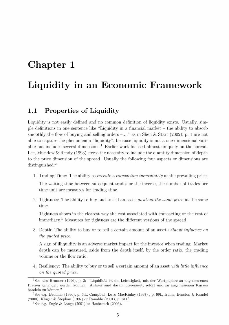
Figure 1.1 shows a static picture of the limit order book. On the horizontal axis the bid
and ask volumes are depicted to the left and to the right, respectively. These volumes may
be different and the sum of the two is a measure for market depth. On the vertical axis the
price is shown. There exist two different prices: the ask price, at which shares are offered,
and the bid price, at which shares are demanded. The price of a trade may lie at the bid or
at the ask price; under certain circumstances also inside the quote. The difference between
bid and ask price is the measure of tightness but it may be expressed in different terms. The
horizontal dimension is the depth and finally the elasticities of the supply and demand curve
capture the resiliency dimension.
hUi
t! hUi
_ hUi
4*@|i_t! VL*4i
4*@|i__ VL*4i t! #iT|_ #iT|
#iT|
A|?itt
5TT*)+it*i?U)
#i4@?_+it*i?U)
Figure 1.1: Different aspects of liquidity in a static image of the limit order book. Based onRanaldo (2001), p. 312.
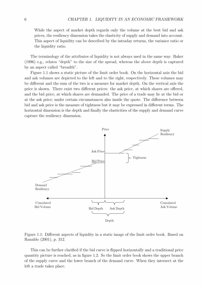
This can be further clarified if the bid curve is flipped horizontally and a traditional price
quantity picture is reached, as in figure 1.2. So the limit order book shows the upper branch
of the supply curve and the lower branch of the demand curve. When they intersect at the
left a trade takes place.
1.1. PROPERTIES OF LIQUIDITY 7
t! hUi
hUi
_ hUi
VL*4i
A|?itt
5TT*)+it*i?U)
#i4@?_+it*i?U)
Figure 1.2: Supply and demand in the limit order book. Based on Ranaldo (2001), p. 312.
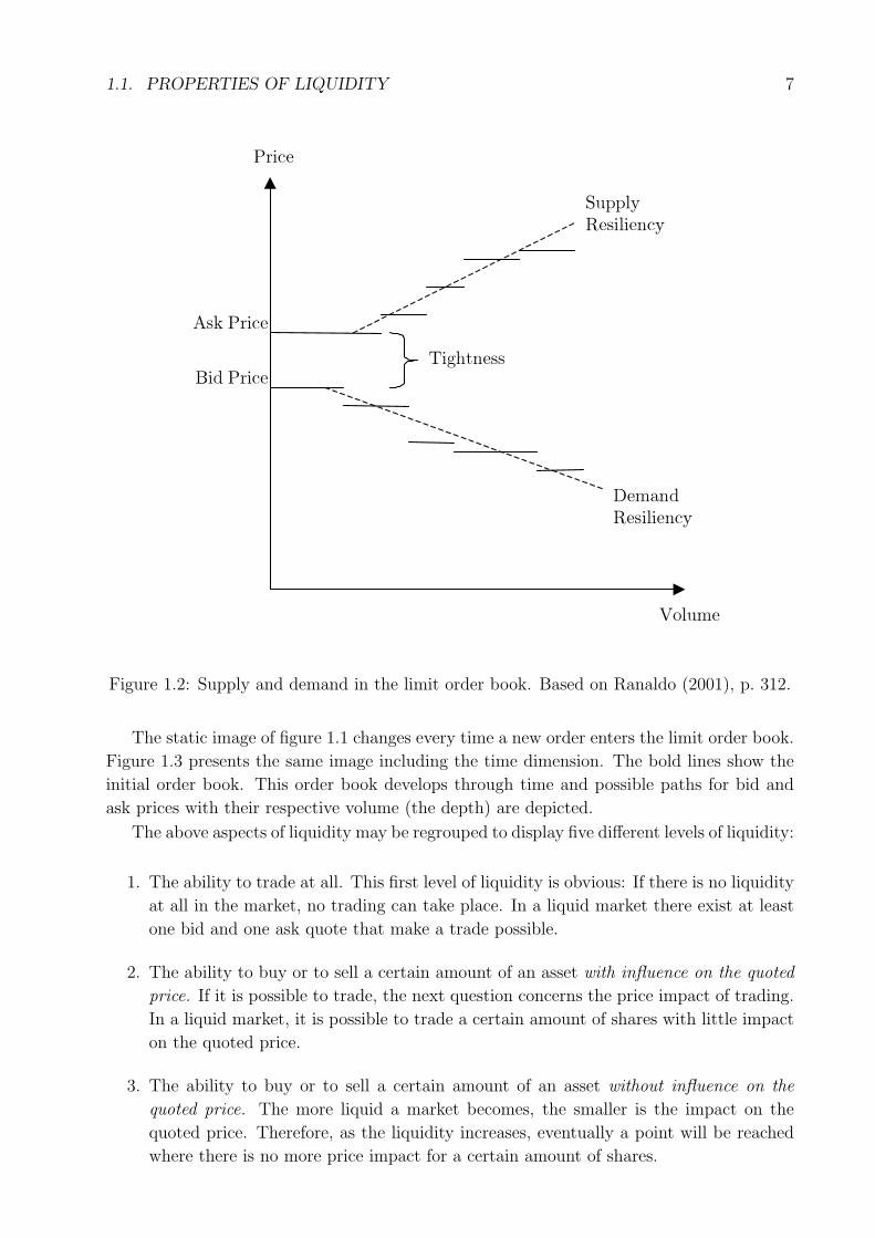
The static image of figure 1.1 changes every time a new order enters the limit order book.
Figure 1.3 presents the same image including the time dimension. The bold lines show the
initial order book. This order book develops through time and possible paths for bid and
ask prices with their respective volume (the depth) are depicted.
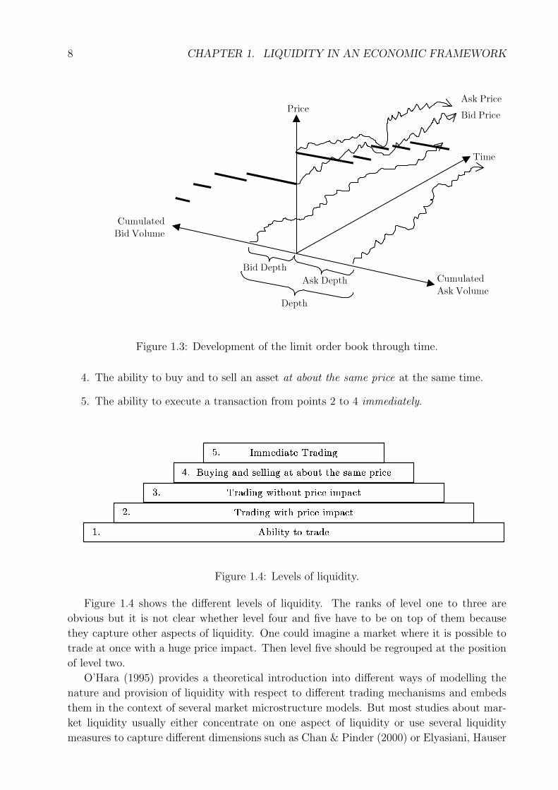
The above aspects of liquidity may be regrouped to display five different levels of liquidity:
1. The ability to trade at all. This first level of liquidity is obvious: If there is no liquidity
at all in the market, no trading can take place. In a liquid market there exist at least
one bid and one ask quote that make a trade possible.
2. The ability to buy or to sell a certain amount of an asset with influence on the quoted
price. If it is possible to trade, the next question concerns the price impact of trading.
In a liquid market, it is possible to trade a certain amount of shares with little impact
on the quoted price.
3. The ability to buy or to sell a certain amount of an asset without influence on the
quoted price. The more liquid a market becomes, the smaller is the impact on the
quoted price. Therefore, as the liquidity increases, eventually a point will be reached
where there is no more price impact for a certain amount of shares.
8 CHAPTER 1. LIQUIDITY IN AN ECONOMIC FRAMEWORK
hUit! hUi_ hUi
4*@|i_t! VL*4i
4*@|i__ VL*4i
t! #iT|_ #iT|
#iT|
A4i
Figure 1.3: Development of the limit order book through time.
4. The ability to buy and to sell an asset at about the same price at the same time.
5. The ability to execute a transaction from points 2 to 4 immediately.
Figure 1.4: Levels of liquidity.
Figure 1.4 shows the different levels of liquidity. The ranks of level one to three are
obvious but it is not clear whether level four and five have to be on top of them because
they capture other aspects of liquidity. One could imagine a market where it is possible to
trade at once with a huge price impact. Then level five should be regrouped at the position
of level two.
O’Hara (1995) provides a theoretical introduction into different ways of modelling the
nature and provision of liquidity with respect to different trading mechanisms and embeds
them in the context of several market microstructure models. But most studies about mar-
ket liquidity usually either concentrate on one aspect of liquidity or use several liquidity
measures to capture different dimensions such as Chan & Pinder (2000) or Elyasiani, Hauser
1.2. LIQUIDITY MEASURES 9
& Lauterbach (2000). Fernandez (1999), p. 1 stresses the need to use different liquidity
measures to capture the different aspects of liquidity. Another possibility is to use multidi-
mensional liquidity measures.
The following section 1.2 gives a summary of the liquidity measures used in literature
that is certainly not complete but should provide an overview of how the problem can be
addressed.
1.2 Liquidity Measures
Liquidity itself is not observable and therefore, has to be proxied by different liquidity mea-
sures. As Baker (1996) states, different liquidity measures lead to conflicting results when
evaluating the liquidity of a financial market.
To get an overview, liquidity measures are separated into one-dimensional and multi-
dimensional ones: One-dimensional liquidity measures take only one variable into account,
whereas the multi-dimensional liquidity measures try to capture different variables in one
measure.
1.2.1 One-dimensional Liquidity Measures
The one-dimensional liquidity measures may be roughly separated into four groups: They
may capture the size of the firm, the volume traded, the time between subsequent trades
or the spread. The liquidity measures related to the firm size are not investigated further
because, in the intraday context, they do not show enough variation to get reasonable results.
They are listed in appendix A.1.
Volume-related Liquidity Measures
The volume-related liquidity measures may be calculated as a certain volume, or quantity of
shares, per time unit. Usually they are used to capture the depth dimension of liquidity, but
there is also a relation to the time dimension since a higher volume in the market leads to a
shorter time needed for trading a predefined amount of shares. Trading volume is carefully
investigated by Lee & Swaminathan (2000) in the context of momentum and value strategies.
If the volume-related liquidity measures are high, this is a sign of high liquidity.
• Trading volume:
Trading volume per time interval (Qt) is incorporated in a lot of liquidity studies4.
Trading volume for time t− 1 until time t is calculated as follows:
Qt =Nt∑i=1
qi (1.1)
4Examples are: Chordia, Roll & Subrahmanyam (2001), Chordia, Subrahmanyam & Anshuman (2001),Elyasiani et al. (2000), George & Hwang (1998), Gervais, Kaniel & Mingelgrin (2001), Greene & Smart(1999), Hasbrouck & Saar (2002), Hasbrouck & Seppi (2001), Kamara & Koski (2001), Karagozoglu (2000),Lee et al. (1993), Lee, Fok & Liu (2001), Lin, Sanger & Booth (1995), Van Ness, Van Ness & Pruitt (2000),and Yang, Li & Liu (2001).
10 CHAPTER 1. LIQUIDITY IN AN ECONOMIC FRAMEWORK
Nt denotes the number of trades between t−1 and t, qi is the number of shares of trade
i. The average trade size is strongly influenced by the institutional frameset. Barclay,
Christie, Harris, Kandel & Schultz (1999) show how the reduction of the minimum
quote size on the NASDAQ reduces average trade size. But, in their paper, they stress
that in line with the smaller trade sizes “the total quoted size in close proximity to
the bid-ask midpoint increases.”5 This discrepancy between the depth at the best bid
and ask quotes and the depth deeper in the order book can be overcome with more
sophisticated liquidity measures described further below.
Gourieroux, Jasiak & Le Fol (1999) calculate the reverse of the volume per time unit,
the volume duration (DurQQ∗t ). This extended duration measure indicates the time
that is needed to trade a certain number of shares Q∗:
DurQQ∗t = inf (DurQ : Qt+DurQ ≥ Qt + Q∗)
= inf
DurQ :
Nt+DurQ∑i=1
qi ≥Nt∑i=1
qi + Q∗
Qt denotes the cumulative number of shares traded until time t, Nt is the number of
trades.
• Turnover6:
Like the trading volume, turnover (Vt) has to be calculated for a specific time interval:
Vt =Nt∑i=1
pi · qi (1.2)
pi denotes the price of trade i. Nt is the number of trades between t − 1 and t. An
example of the turnover per time unit in use is the article by Chan, Chung & Fong
(2002) who investigate the volume of options and stocks to filter out its informational
contents. They refine the turnover to “net-trade volume” , which is calculated as
buyer-initiated volume minus seller-initiated volume. Sometimes turnover is refined to
a so called “relative turnover” which relates turnover to the free float of a stock as in
Brunner (1996), p. 17.
Gourieroux et al. (1999) propose the reverse of the turnover, the turnover duration
(DurV V ∗t ) to take the time into account that is needed to trade a certain turnover
V ∗:7
5Barclay et al. (1999), p. 3.6As well as the trading volume, turnover is frequently used as in Chordia, Roll & Subrahmanyam (2001),
Chordia, Subrahmanyam & Anshuman (2001), Chordia & Swaminathan (2000) , Gervais et al. (2001),Fleming & Remolona (1999), Hasbrouck & Saar (2002), Hasbrouck & Seppi (2001), Jones & Lipson (1999),Kamara & Koski (2001), Lee & Swaminathan (2000), and Lin et al. (1995).
7In Gourieroux et al. (1999), p. 207 the turnover duration is called “capital duration”.
1.2. LIQUIDITY MEASURES 11
DurV V ∗t = inf (DurV : Vt+DurV ≥ Vt + V ∗)
= inf
(DurV :
Nt+DurV∑pi·
i=1
qi ≥Nt∑
pi·i=1
qi + V ∗)
Trading volume and turnover only need trades as data input which makes them easy to
calculate. The turnover per time unit has the advantage that it makes different shares
comparable to each other. It is not biased by the absolute share price as e.g. Irvine et al.
(2000) point out.
The following three liquidity measures exist at any point in time, even if no transaction
takes place. Only the first level of liquidity – the existence of a bid and an ask quote – has
to be reached. Therefore, it is not necessary to calculate these liquidity proxies for a specific
period.
• Depth:
Dt = qAt + qB
t (1.3)
The market depth in time t, Dt, which is also referred to as “quantity depth” as in
Huberman & Halka (2001) or “volume depth” as in Brockman & Chung (2000) is
calculated as the sum of bid and ask volume in time t. qAt and qB
t refer to the best bid
and the best ask volume in the order book. Corwin (1999) shows that market depth
differs significantly among the NYSE specialist firms, and Corwin & Lipson (2000)
investigate depth around trading halts. Greene & Smart (1999) look at abnormal
depth due to liquidity trading.8
The market depth may be divided by two and, therefore, modified to an average depth
of the bid and the ask depth as in Chordia, Roll & Subrahmanyam (2001), Goldstein
& Kavajecz (2000), or Sarin, Shastri & Shastri (1996).
The depth of the bid- and the ask-sides of the limit order book do not necessarily move
in common and may therefore be investigated separately as in Kavajecz (1999) and
Kavajecz & Odders-White (2001).
• Log depth:
To improve the distributional properties of the depth the log depth (Dlog t) may be
used, as in Butler, Grullon & Weston (2002).
Dlogt = ln(qAt ) + ln(qB
t ) = ln(qAt · qB
t ) (1.4)
Log depth is simply the sum of the logarithms of the best bid and ask volume in the
order book.
8Besides the articles mentioned, depth is also used in Lee et al. (1993) and Van Ness et al. (2000).
12 CHAPTER 1. LIQUIDITY IN AN ECONOMIC FRAMEWORK
• Dollar depth:
Dollar depth (D$t) is usually calculated as the average of the quoted bid and ask
depths in currency terms, analogously to the average depth.9
D$t =qAt · pA
t + qBt · pB
t
2(1.5)
pAt refers to best ask price at time t and pB
t to the best bid price at time t. Like turnover,
dollar depth has the advantage that it makes liquidity of different stocks comparable
to each other. It is important not to intermingle the number of shares that can be
traded at a certain price with their respective amount of money. But turnover is not
a priori the better liquidity measure than volume. For a retail investor, the turnover
of one share at 20’000 CHF may be less liquid than the turnover of 20 shares at 1’000
CHF.
All these depth measures only take the depth at the best bid and ask quotes into con-
sideration. Larger orders10 cannot completely be executed at the best bid and ask prices
and therefore have to “walk the book”. This issue is considered in the more sophisticated
liquidity measures below.
Time-related Liquidity Measures
Time-related liquidity measures indicate how often transactions or orders take place. There-
fore, high values of these measures indicate high liquidity.
• Number of transactions per time unit:
Like the trading volume, the number of trades is a widely used liquidity measure.11
Nt (1.6)
It counts the number of trades between t− 1 and t. The number of transactions may
be reversed to waiting time between trades
WTt =1
N − 1
N∑i=2
tri − tri−1.
tri denotes the time of the trade and tri−1 the time of the trade before.12 Therefore,
waiting time for a specific time space has to be calculated as an average time be-
tween two trades. Waiting time is, for example, investigated by Peng (2001). Since it
9See e.g. Brockman & Chung (2000), Chordia, Roll & Subrahmanyam (2001), p. 505 or Hasbrouck &Seppi (2001).
10Bacidore, Battalio & Jennings (2002) estimate the fraction of NYSE system market orders to be greaterthan the quoted depth at 16% which equals about 23% of the order’s value. This sample does not includeorders handled by floor brokers.
11Bacidore (1997), Chordia, Roll & Subrahmanyam (2001), Christie & Schultz (1998), Jones & Lipson(1999), Kamara & Koski (2001), or Kavajecz & Odders-White (2001) count the number of trades per day,Hasbrouck & Seppi (2001) for a 15 minute interval and daily.
12See e.g. Gourieroux et al. (1999) or Ranaldo (2003).
1.2. LIQUIDITY MEASURES 13
yields essentially the same information as the number of trades, waiting time between
trades will not be investigated further. Instead of the waiting time between trades, the
waiting time between subsequent orders may be calculated as in Ranaldo (2004). For
consistency, this is calculated as the number of orders per time unit.
The number of transactions and the waiting time show the difference of trading taking
place in a few large trades or in a huge number of small trades. But these measures are
unable to compare liquidity of stocks whose prices differ significantly from each other.
• Number of orders per time unit:
Similar to the number of transactions per time unit, the number of orders (NOt) counts
the orders inserted into the limit order book within the time interval from t− 1 until
t:
NOt (1.7)
The impact of the number of orders on return volatility is investigated by Walsh (1998).
Spread-related Liquidity Measures
The difference between the ask and the bid price and its related measures gives an approxi-
mation of the cost incurred when trading. In addition to fees and taxes, the trader has to pay
the spread as cost for the immediate execution of a trade. Most studies investigate spreads
on a daily basis: Acker, Stalker & Tonks (2002) e.g. examine the determinants of bid-ask
spreads and their behavior around corporate earning announcement dates. The spread is
used to determine where price discovery takes place in Harris, McInish & Wood (2002), a
study that compares trading at different stock exchanges.
The smaller all the spread-related liquidity measures are, the more liquid is the market.
• Absolute spread, dollar spread or quoted spread:
Sabst = pAt − pB
t (1.8)
The absolute spread is the difference between the lowest ask price and the highest bid
price. This measure is always positive and its lower limit is the minimum tick size.
Chordia, Roll & Subrahmanyam (2001) use this measure in their study of the NYSE
and Grammig, Schiereck & Theissen (2001) with data of the German stock market.13
A somewhat different approach is used by Hasbrouck (1999): He models the spread
out of different stochastic variables for the bid and the ask price.
The expression “quoted spread” is ambiguous and refers not only to the difference of the
best bid and the best ask price but also to the quoted spread of a single market maker,
who quotes bid and ask prices. It is intensively investigated for the whole market
and for single market makers in Barclay et al. (1999) who analyze the impact of the
NASDAQ market reforms of 1997, which ended the collusion among market makers
13Other articles incorporating the spread are Bacidore (1997), Breedon & Holland (1997), Brockman &Chung (2000), Chung & Van Ness (2001), Clyman, Allen & Jaycobs (1997), Clyman & Jaycobs (1998),Greene & Smart (1999), Hasbrouck & Saar (2002), Hasbrouck & Seppi (2001), Kavajecz & Odders-White(2001), Lee et al. (1993), Lin et al. (1995), Ranaldo (2002), or Van Ness et al. (2000).
14 CHAPTER 1. LIQUIDITY IN AN ECONOMIC FRAMEWORK
to artificially inflate the spreads. The quoted spread differs also across the NYSE
specialist firms as Corwin (1999) shows. Another study using individual dealer’s data
is Christie & Schultz (1998) who investigate the liquidity provision during the 1991
market break, when the index fell over 4%. Furthermore, it is possible to compare the
quotes of the specialists at the NYSE or the limit order book quotes of a single market
maker as it has been done for the NYSE14 or the London Stock Exchange.15 In the
present dissertation it is not possible to compare the quoted spreads of different market
participants because the SWX is not allowed to publicly release this sort of data.
Karagozoglu (2000) divides the quoted spread by two but has to calculate it out of the
average price reversals because quote data is not available in the futures market. The
quoted spread is largely determined by the minimum tick size, which is investigated in
Ball & Chordia (2001). Since the minimum tick size is not constant at the SWX but
depends on the stock price, stock prices influence the absolute spread.
• Log absolute spread:
LogSabst = ln(Sabst) = ln(pAt − pB
t ) (1.9)
Like the log depth, the absolute spread may be logarithmized to improve its distribu-
tional properties. It is used in Hamao & Hasbrouck (1995) because its distribution is
closer to a normal than the absolute spread and, therefore, mathematically easier to
use.
• Relative spread or proportional spread calculated with mid price:
SrelMt =pA
t − pBt
pMt
=2 · (pA
t − pBt
)
pAt + pB
t
(1.10)
pMt denotes the mid price which is calculated as
pAt +pB
t
2. The relative spread is the
liquidity measure most extensively studied because it is easy to calculate and because it
makes spreads of different stocks comparable to each other.16 Sometimes this measure
is also referred to as “inside spread” as in Levin & Wright (1999). Another advantage
is that it may be calculated even if no trade takes place, in contrast to the relative
spread calculated with the last trade (see below).
• Relative spread calculated with last trade:
Srelpt =pA
t − pBt
pt
(1.11)
14Studies about the NYSE are Battalio, Greene & Jennings (1998), Chung, Van Ness & Van Ness (1999),Goldstein & Kavajecz (2000), and Kavajecz (1999).
15Studies using data from the London Stock Exchange are Levin & Wright (1999) and Menyah & Paudyal(2000).
16Acker et al. (2002), Brockman & Chung (2000), Chordia, Roll & Subrahmanyam (2001), Chung & VanNess (2001) Corwin (1999), Elyasiani et al. (2000), Gervais et al. (2001), Goldstein & Kavajecz (2000),Greene & Smart (1999), Hasbrouck & Saar (2002), Jones & Lipson (1999), Kavajecz (1999), Kluger &Stephan (1997), Lin et al. (1995), Menyah & Paudyal (2000), Ranaldo (2003), Sarin et al. (1996), Van Nesset al. (2000), or Yang et al. (2001) use the relative spread.
1.2. LIQUIDITY MEASURES 15
pt denotes the last paid price of the asset before time t. This liquidity measure is
used e.g. in Fleming & Remolona (1999). On the one hand, this second version of the
relative spread has the advantage of taking a moving market into account, because pt
may be at the ask price in an upward moving market, whereas it will be at the bid price
in a downward moving market. On the other hand, the paid price pt has to be known
before pAt or pB
t are quoted. If the last trade has occurred long before the current
absolute spread is measured, the traded price as well as Srelpt may be irrelevant for
the actual market situation.
The relative spread is calculated with the bid price in the denominator in Loderer &
Roth (2001). The authors state that this spread measure is arbitrarily chosen and
that they could have equally selected the relative spread with the mid price in the
denominator. Therefore, the relative spread with the bid price in the denominator
is not investigated further. Amihud & Mendelson (1991) add to the bid price in the
denominator the accrued interest to measure liquidity of Treasury bills and notes. This
is done in order to account for the realizable liquidation price of these fixed income
securities.
• Relative spread of log prices:
Srellogt = ln(pAt )− ln(pB
t ) = ln(pA
t
pBt
) (1.12)
Srellogt is calculated analogously to the log return of an asset. It is compared to other
liquidity measures in Hasbrouck & Seppi (2001) who find only modest common factors
in liquidity after removing the time-of-day effects.
• Log relative spread of log prices:
LogSrellogt = ln (Srellogt) = ln(ln(pA
t
pBt
)) (1.13)
LogSrellogt is used to generate “better” distributions of the spread measure. All the
previous spread measures have a strongly skewed distribution which complicates cal-
culations. The log relative spread of log prices is much more symmetrically distributed
and is therefore easier to approximate by a normal distribution.17
• Effective spread:
Seff t=∣∣pt − pM
t
∣∣ (1.14)
pt denotes the last traded price before time t and the mid price pMt is calculated
as above. The effective spread is a different spread concept: If the effective spread
is smaller than half the absolute spread, this reflects trading within the quotes.18
Sometimes the effective spread and all the following related measures may be multiplied
by two to make them better comparable to the other spread measures, as in Barclay
17See Dacorogna, Gencay, Muller, Olsen & Pictet (2001), p. 45.18See Chordia, Roll & Subrahmanyam (2000), Chordia, Roll & Subrahmanyam (2001), p. 506, Christie &
Schultz (1998), or Hasbrouck & Seppi (2001).
16 CHAPTER 1. LIQUIDITY IN AN ECONOMIC FRAMEWORK
et al. (1999), p. 14, Bacidore (1997), Bacidore et al. (2002), Breedon & Holland (1997),
Jones & Lipson (1999), or Lin et al. (1995). In Lee et al. (1993) this doubled effective
spread is weighted with the trade size to get an average effective spread for a certain
period. This yields similar results as weighting with the number of trades does. With
the use of the effective spread, Battalio et al. (1998) calculate a liquidity premium:
LPt = I · (pt − pMt
)where I is the direction of trade indicator. I equals 1 for buyer
initiated trades and -1 for seller initiated trades. This liquidity premium is positive if
the buyer pays more or if the seller pays less than the spread midpoint.
• Relative effective spread calculated with last trade:
Seffrelpt=
∣∣pt − pMt
∣∣pt
(1.15)
Again, the relative measure allows comparability across different stocks.19 Also the
relative effective spread may be doubled to compare it to other relative spread mea-
sures.20
• Relative effective spread calculated with mid price:
SeffrelM t=
∣∣pt − pMt
∣∣pMt
(1.16)
As with the relative spread, the relative effective spread can be calculated with the
mid price in the denominator as in Grammig et al. (2001) or Ranaldo (2003). Corwin
(1999) uses this measure multiplied by 200.
To make data of different stocks comparable to each other it is always useful to rely on
relative spread measures. All the spread measures take only the best bid and ask prices
into consideration. But in the market there are usually multiple spreads, each relating to a
different volume of shares. Out of the limit order book of the Swiss Exchange it is possible
to construct supply and demand curves, which give additional insights into the liquidity of
the stock market.21
1.2.2 Multi-dimensional Liquidity Measures
Multi-dimensional liquidity measures combine properties of different one-dimensional liquid-
ity measures. Fifteen measures shall be explained in this section. The first four combine
spread in the numerator and volume in the denominator. Therefore, a high liquidity mea-
sures denotes low liquidity.
• Quote slope:
QSt =Sabst
Dlogt
=pA
t − pBt
ln (qAt ) + ln (qB
t )(1.17)
19The relative effective spread is used in Chordia et al. (2000) and Chordia, Roll & Subrahmanyam (2001).20See Barclay et al. (1999), Goldstein & Kavajecz (2000), Lin et al. (1995), Schultz (2000), or Theissen
(2002).21See e.g. Chan & Pinder (2000), p. 485 or Corwin & Lipson (2000).
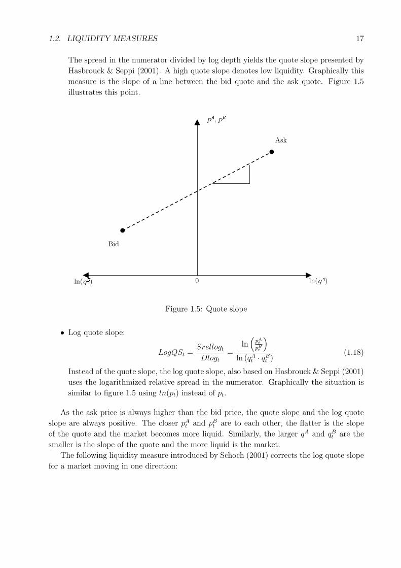
1.2. LIQUIDITY MEASURES 17
The spread in the numerator divided by log depth yields the quote slope presented by
Hasbrouck & Seppi (2001). A high quote slope denotes low liquidity. Graphically this
measure is the slope of a line between the bid quote and the ask quote. Figure 1.5
illustrates this point.
*?E^
Tc T
*?E^
t!
_
f
Figure 1.5: Quote slope
• Log quote slope:
LogQSt =Srellogt
Dlogt
=ln
(pA
t
pBt
)
ln (qAt · qB
t )(1.18)
Instead of the quote slope, the log quote slope, also based on Hasbrouck & Seppi (2001)
uses the logarithmized relative spread in the numerator. Graphically the situation is
similar to figure 1.5 using ln(pt) instead of pt.
As the ask price is always higher than the bid price, the quote slope and the log quote
slope are always positive. The closer pAt and pB
t are to each other, the flatter is the slope
of the quote and the market becomes more liquid. Similarly, the larger qA and qBt are the
smaller is the slope of the quote and the more liquid is the market.
The following liquidity measure introduced by Schoch (2001) corrects the log quote slope
for a market moving in one direction:
18 CHAPTER 1. LIQUIDITY IN AN ECONOMIC FRAMEWORK
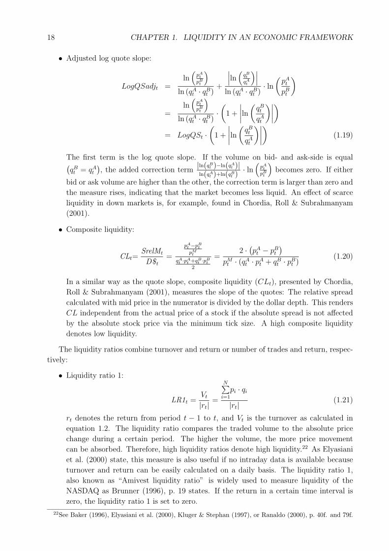
• Adjusted log quote slope:
LogQSadjt =ln
(pA
t
pBt
)
ln (qAt · qB
t )+
∣∣∣ln(
qBt
qAt
)∣∣∣ln (qA
t · qBt )· ln
(pA
t
pBt
)
=ln
(pA
t
pBt
)
ln (qAt · qB
t )·(
1 +
∣∣∣∣ln(
qBt
qAt
)∣∣∣∣)
= LogQSt ·(
1 +
∣∣∣∣ln(
qBt
qAt
)∣∣∣∣)
(1.19)
The first term is the log quote slope. If the volume on bid- and ask-side is equal(qBt = qA
t
), the added correction term
|ln(qBt )−ln(qA
t )|ln(qA
t )+ln(qBt )
· ln(
pAt
pBt
)becomes zero. If either
bid or ask volume are higher than the other, the correction term is larger than zero and
the measure rises, indicating that the market becomes less liquid. An effect of scarce
liquidity in down markets is, for example, found in Chordia, Roll & Subrahmanyam
(2001).
• Composite liquidity:
CLt=SrelMt
D$t
=
pAt −pB
t
pMt
qAt ·pA
t +qBt ·pB
t
2
=2 · (pA
t − pBt
)
pMt · (qA
t · pAt + qB
t · pBt )
(1.20)
In a similar way as the quote slope, composite liquidity (CLt), presented by Chordia,
Roll & Subrahmanyam (2001), measures the slope of the quotes: The relative spread
calculated with mid price in the numerator is divided by the dollar depth. This renders
CL independent from the actual price of a stock if the absolute spread is not affected
by the absolute stock price via the minimum tick size. A high composite liquidity
denotes low liquidity.
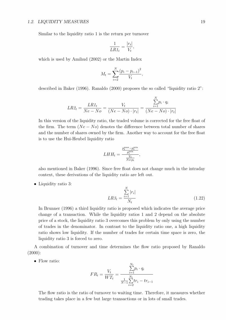
The liquidity ratios combine turnover and return or number of trades and return, respec-
tively:
• Liquidity ratio 1:
LR1t =Vt
|rt| =
N∑i=1
pi · qi
|rt| (1.21)
rt denotes the return from period t − 1 to t, and Vt is the turnover as calculated in
equation 1.2. The liquidity ratio compares the traded volume to the absolute price
change during a certain period. The higher the volume, the more price movement
can be absorbed. Therefore, high liquidity ratios denote high liquidity.22 As Elyasiani
et al. (2000) state, this measure is also useful if no intraday data is available because
turnover and return can be easily calculated on a daily basis. The liquidity ratio 1,
also known as “Amivest liquidity ratio” is widely used to measure liquidity of the
NASDAQ as Brunner (1996), p. 19 states. If the return in a certain time interval is
zero, the liquidity ratio 1 is set to zero.
22See Baker (1996), Elyasiani et al. (2000), Kluger & Stephan (1997), or Ranaldo (2000), p. 40f. and 79f.
1.2. LIQUIDITY MEASURES 19
Similar to the liquidity ratio 1 is the return per turnover
1
LR1t
=|rt|Vt
,
which is used by Amihud (2002) or the Martin Index
Mt =N∑
i=2
(pi − pi−1)2
Vt
,
described in Baker (1996). Ranaldo (2000) proposes the so called “liquidity ratio 2”:
LR2t =LR1t
Ne−No=
Vt
(Ne−No) · |rt| =
N∑i=1
pi · qi
(Ne−No) · |rt|
In this version of the liquidity ratio, the traded volume is corrected for the free float of
the firm. The term (Ne−No) denotes the difference between total number of shares
and the number of shares owned by the firm. Another way to account for the free float
is to use the Hui-Heubel liquidity ratio
LHHt =
pmaxt −pmin
t
pmint
Vt
No·pt
,
also mentioned in Baker (1996). Since free float does not change much in the intraday
context, these derivations of the liquidity ratio are left out.
• Liquidity ratio 3:
LR3t =
N∑i=1
|ri|Nt
(1.22)
In Brunner (1996) a third liquidity ratio is proposed which indicates the average price
change of a transaction. While the liquidity ratios 1 and 2 depend on the absolute
price of a stock, the liquidity ratio 3 overcomes this problem by only using the number
of trades in the denominator. In contrast to the liquidity ratio one, a high liquidity
ratio shows low liquidity. If the number of trades for certain time space is zero, the
liquidity ratio 3 is forced to zero.
A combination of turnover and time determines the flow ratio proposed by Ranaldo
(2000):
• Flow ratio:
FRt =Vt
WTt
=
Nt∑i=1
pi · qi
1N−1
Nt∑i=2
tri − tri−1
The flow ratio is the ratio of turnover to waiting time. Therefore, it measures whether
trading takes place in a few but large transactions or in lots of small trades.
20 CHAPTER 1. LIQUIDITY IN AN ECONOMIC FRAMEWORK
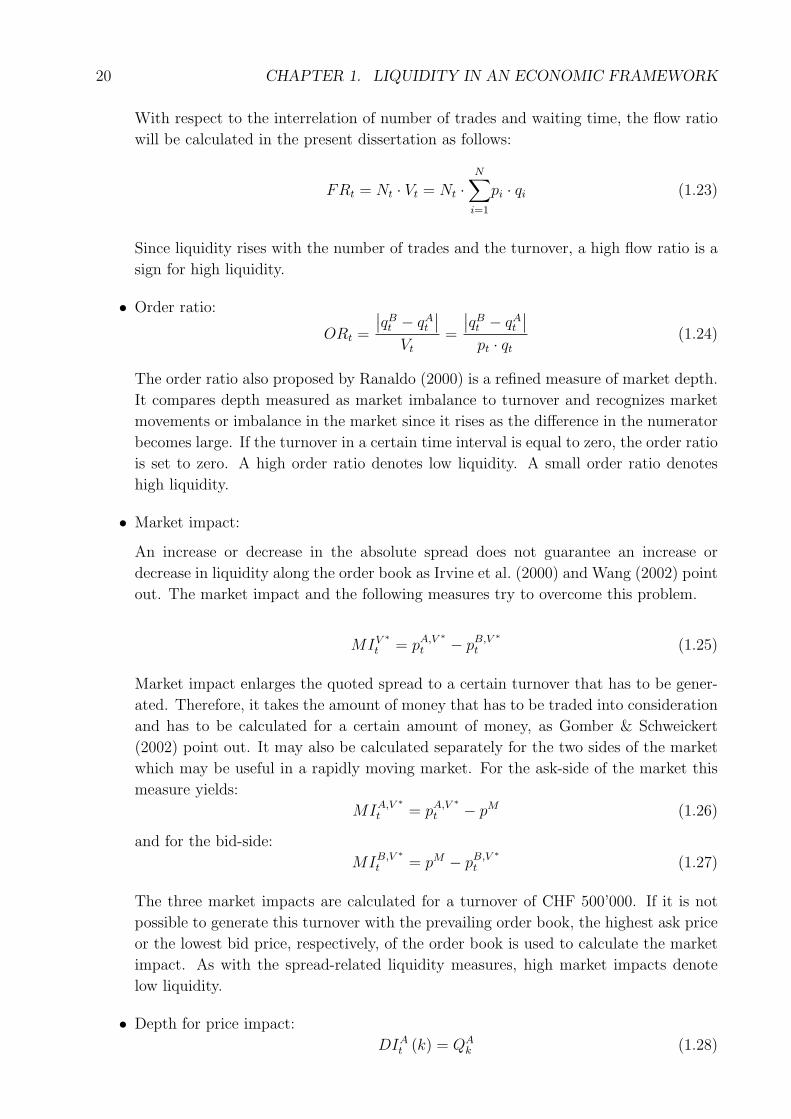
With respect to the interrelation of number of trades and waiting time, the flow ratio
will be calculated in the present dissertation as follows:
FRt = Nt · Vt = Nt ·N∑
i=1
pi · qi (1.23)
Since liquidity rises with the number of trades and the turnover, a high flow ratio is a
sign for high liquidity.
• Order ratio:
ORt =
∣∣qBt − qA
t
∣∣Vt
=
∣∣qBt − qA
t
∣∣pt · qt
(1.24)
The order ratio also proposed by Ranaldo (2000) is a refined measure of market depth.
It compares depth measured as market imbalance to turnover and recognizes market
movements or imbalance in the market since it rises as the difference in the numerator
becomes large. If the turnover in a certain time interval is equal to zero, the order ratio
is set to zero. A high order ratio denotes low liquidity. A small order ratio denotes
high liquidity.
• Market impact:
An increase or decrease in the absolute spread does not guarantee an increase or
decrease in liquidity along the order book as Irvine et al. (2000) and Wang (2002) point
out. The market impact and the following measures try to overcome this problem.
MIV ∗t = pA,V ∗
t − pB,V ∗t (1.25)
Market impact enlarges the quoted spread to a certain turnover that has to be gener-
ated. Therefore, it takes the amount of money that has to be traded into consideration
and has to be calculated for a certain amount of money, as Gomber & Schweickert
(2002) point out. It may also be calculated separately for the two sides of the market
which may be useful in a rapidly moving market. For the ask-side of the market this
measure yields:
MIA,V ∗t = pA,V ∗
t − pM (1.26)
and for the bid-side:
MIB,V ∗t = pM − pB,V ∗
t (1.27)
The three market impacts are calculated for a turnover of CHF 500’000. If it is not
possible to generate this turnover with the prevailing order book, the highest ask price
or the lowest bid price, respectively, of the order book is used to calculate the market
impact. As with the spread-related liquidity measures, high market impacts denote
low liquidity.
• Depth for price impact:
DIAt (k) = QA
k (1.28)
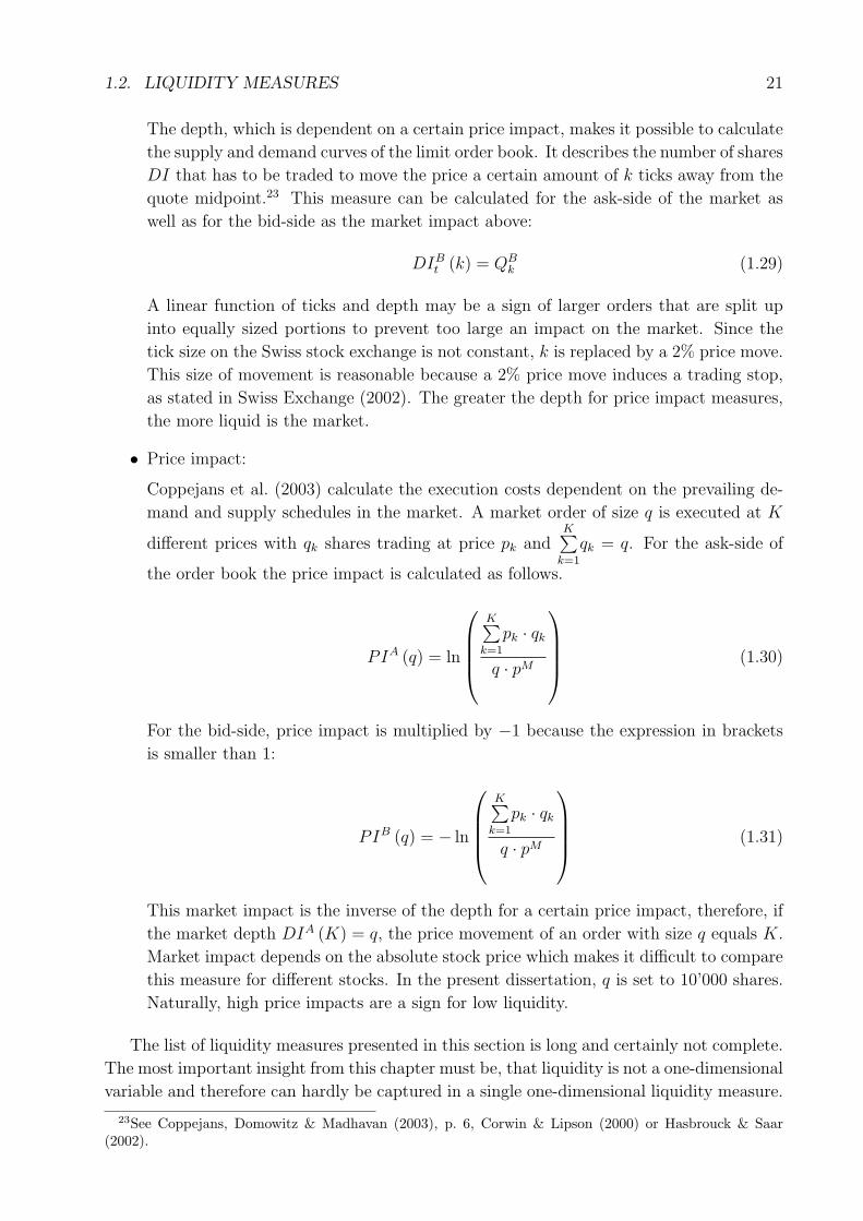
1.2. LIQUIDITY MEASURES 21
The depth, which is dependent on a certain price impact, makes it possible to calculate
the supply and demand curves of the limit order book. It describes the number of shares
DI that has to be traded to move the price a certain amount of k ticks away from the
quote midpoint.23 This measure can be calculated for the ask-side of the market as
well as for the bid-side as the market impact above:
DIBt (k) = QB
k (1.29)
A linear function of ticks and depth may be a sign of larger orders that are split up
into equally sized portions to prevent too large an impact on the market. Since the
tick size on the Swiss stock exchange is not constant, k is replaced by a 2% price move.
This size of movement is reasonable because a 2% price move induces a trading stop,
as stated in Swiss Exchange (2002). The greater the depth for price impact measures,
the more liquid is the market.
• Price impact:
Coppejans et al. (2003) calculate the execution costs dependent on the prevailing de-
mand and supply schedules in the market. A market order of size q is executed at K
different prices with qk shares trading at price pk andK∑
k=1
qk = q. For the ask-side of
the order book the price impact is calculated as follows.
PIA (q) = ln
K∑k=1
pk · qk
q · pM
(1.30)
For the bid-side, price impact is multiplied by −1 because the expression in brackets
is smaller than 1:
PIB (q) = − ln
K∑k=1
pk · qk
q · pM
(1.31)
This market impact is the inverse of the depth for a certain price impact, therefore, if
the market depth DIA (K) = q, the price movement of an order with size q equals K.
Market impact depends on the absolute stock price which makes it difficult to compare
this measure for different stocks. In the present dissertation, q is set to 10’000 shares.
Naturally, high price impacts are a sign for low liquidity.
The list of liquidity measures presented in this section is long and certainly not complete.
The most important insight from this chapter must be, that liquidity is not a one-dimensional
variable and therefore can hardly be captured in a single one-dimensional liquidity measure.
23See Coppejans, Domowitz & Madhavan (2003), p. 6, Corwin & Lipson (2000) or Hasbrouck & Saar(2002).
22 CHAPTER 1. LIQUIDITY IN AN ECONOMIC FRAMEWORK
For a global liquidity measure, certainly one of the multi-dimensional liquidity measures has
to be used. According to Amihud (2002), it is doubtful whether there is one single measure
that captures all aspects of liquidity. On the other hand, the one-dimensional measures may
give insight into specific questions of market liquidity which more complicated measures are
unable to furnish.
For the empirical part, the 31 liquidity measures from the numbered equations will be
used. Some more liquidity measures left out can be found in appendix A.
Chapter 2
Data and Institutional Setting
A brief description of the institutional setting of the Swiss Exchange is necessary to under-
stand the trading mechanism and how liquidity is provided. It takes place in the following
section. In section 2.2, I describe the data used throughout the dissertation, and how it had
to be preprocessed.
2.1 The Limit Order Book of the Swiss Exchange1
The Swiss Exchange is organized as a limit order book. For the trading of ordinary shares
no market makers provide liquidity. The market is purely order driven which means that
liquidity in this market is entirely dependent on public limit orders.
The Swiss Exchange provides so-called “order history reports” (OHR), which makes it
possible to reconstruct the order book for every point in time. Kavajecz (1999) describes,
in a clear and consistent way, how the limit order book may be constructed out of order
history reports. Using an autoregressive conditional duration (ACD) model, Coppejans &
Domowitz (2002) give an interesting insight into the mechanisms at work in a limit order
book. They use data from the OMX futures contract on the Swedish stock index. In this
market, the trading organization is simpler than the Swiss Exchange because neither opening
nor closing auctions exist.
Every single event is entered into the order book and appears, therefore, in the order
history report. An order that is matched against several other orders appears several times
in the OHR which means that the number of events in the OHR is much larger than the
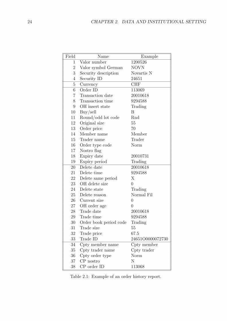
number of orders. Table 2.1 summarizes the information provided by the OHR and gives an
example.
Fields 1 to 4 describe the security. They contain the same information and, therefore,
three of them are redundant. In this case it is the Novartis registered share.
Field five denotes the currency in which the asset is traded. Throughout the sample the
currency is CHF.
The following fields 6 to 19 concern the insertion of the order:
1The main sources for this section are the General Conditions and the Directives which concretize theGeneral Conditions of the Swiss Exchange. They are available via the homepage www.swx.com. See SwissExchange (2001a), Swiss Exchange (2001b), Swiss Exchange (2001c), and Swiss Exchange (2002).
23
24 CHAPTER 2. DATA AND INSTITUTIONAL SETTING
Field Name Example1 Valor number 12005262 Valor symbol German NOVN3 Security description Novartis N4 Security ID 246515 Currency CHF6 Order ID 1130697 Transaction date 200106188 Transaction time 92945889 OH insert state Trading
10 Buy/sell B11 Round/odd lot code Rnd12 Original size 5513 Order price 7014 Member name Member15 Trader name Trader16 Order type code Norm17 Nostro flag18 Expiry date 2001073119 Expiry period Trading20 Delete date 2001061821 Delete time 929458822 Delete same period X23 OH delete size 024 Delete state Trading25 Delete reason Normal Fil26 Current size 027 OH order age 028 Trade date 2001061829 Trade time 929458830 Order book period code Trading31 Trade size 5532 Trade price 67.533 Trade ID 24651O000007273034 Cpty member name Cpty member35 Cpty trader name Cpty trader36 Cpty order type Norm37 CP nostro N38 CP order ID 113068
Table 2.1: Example of an order history report.
2.1. THE LIMIT ORDER BOOK OF THE SWISS EXCHANGE 25
Field 7 shows the order insertion date: June 18, 2001. Field 8 is the order insertion time:
9:29 a.m., 45.88 seconds.
Field 9 gives the state of the exchange when the order was entered. Possible states of
the exchange are pre-opening, pre-opening auction and trading. The pre-opening starts at 6
a.m. and lasts until 9 a.m. In this period orders can be inserted but no trades are executed.
The pre-opening auction takes place after 9 a.m. Afterwards, there is continuous trading
until 5.20 p.m when the exchange switches again to the pre-opening state before the closing
auction takes place at 5.30 p.m. After the closing auction there is again a pre-opening period
until 10 p.m. where orders may be inserted or modified. During continuous trading there is
an automatic interruption of trading for 15 minutes if the potential follow-up price deviates
by 2% or more from the reference price. During this break the exchange is again in the
pre-opening state and it ends with a pre-opening auction. The example order was inserted
during the trading state.
Field 11 indicates whether the size inserted is a round or an odd lot. Since the size of
a round lot in equity trading is one share and it is impossible to trade fractions of shares,
there are no odd lots.
Field 10, 12, and 13 indicate that it is an order to buy 55 shares at CHF 70 or cheaper.
Field 14 and 15 are left blank for data protection reasons. The SWX has access to these
fields to investigate cases of insider trading. In this paper, the deletion of the member name
as well as the counterparty in fields 34 and 35 prevents comparison of quotes or other market
variables across market participants as it is, for example, done in Barclay et al. (1999).
In field 16 the following different orders may be inserted into the order book:
• Normal Order: A normal order is an order to buy or to sell a certain number of shares.
Two types of normal orders exist:
– Market Order: No price is indicated and the order is executed at the prevailing
market price.
– Limit Order: The price is indicated and the order has to be executed at or better
than the indicated price.
• Hidden Size Order: A larger order may be placed as hidden size order. Only part of
it is visible to the other market participants but it is marked as a hidden size order.
The whole order must exceed CHF 3 mio. for SMI shares and CHF 1 mio. for other
stocks. The hidden part of the order has the same time priority as the visible part. The
minimum visible size of a hidden size order is 100 round lots – therefore, 100 shares.
• Accept Order: The accept order immediately accepts all orders in the order book that
correspond to its attributes. If the accept order is not (or only partially) executed, the
whole order (or the remaining part) is cancelled.
• Fill or Kill Order: The fill or kill order must be executed as a whole. Otherwise it is
cancelled.
• Conditional Order: This sort of order remains invisible for other market participants
unless a so called “trigger price” is reached and the order appears in the order book.
Three forms of conditional order can be distinguished:
26 CHAPTER 2. DATA AND INSTITUTIONAL SETTING
– On Stop Order: When the trigger price is reached, the trading system creates a
market order to buy.
– Stop Loss Order: When the trigger price is reached, the trading system creates a
market order to sell.
– Stop Limit Order: When the trigger price is reached, the trading system creates
a limit order to buy or to sell.
Field 17 indicates whether the trade is for a bank’s own position (nostro) or not. Field
18 and 19 show the expiration of an order if it is not cancelled before.
The fields 20 to 33 describe the disappearance of the order from the order book:
Field 20 to 22 indicate the moment when the order disappeared from the order book.
Field 22 shows an X if it is deleted in the same period. This means immediately if during the
trading state of the exchange or in the same pre-opening period. As the order was traded in
the same moment as it was inserted, it was a “marketable limit order”. Field 23 shows the
size of the order that was deleted and not traded.
Every order has to disappear from the order book, which may take place due to several
reasons, as field 25 shows:
• Full match with another order: If an order can be fully matched with another order,
it disappears from the order book. The order book may also indicate “Normal Fil”
which means that the order was merged with other orders to be executed.
• Partial match with another order: If an order can only be partially matched with
another order, the remaining part usually stays in the order book. Only in the case of
an accept order is the remaining part cleared.
• Cancellation of an order: Any order may be cancelled from the order book by request
of the member who inserted it.
• Expiration of an order: To any order an expiration time and date may be added when
the order is inserted.
Trading takes only place in the first two possibilities. But one should keep in mind that
even if no trading takes place, orders may affect the liquidity of the market.
From field 34 onwards, the counterparty of the trade is identified.
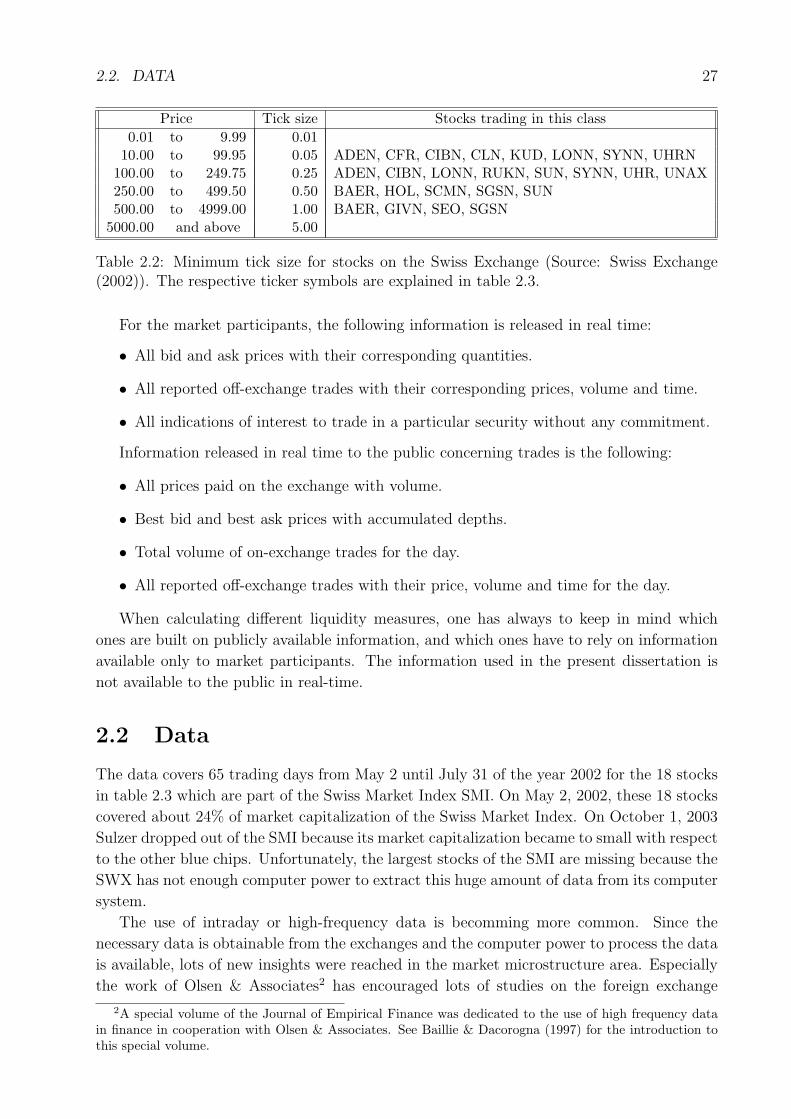
One important determinant of the size of the absolute spread is the minimum tick size
which depends, on the Swiss Exchange, on the absolute stock price. In table 2.2 the minimum
price increments for the Swiss Exchange are shown with there respective price ranges. The
stocks which are used in the present dissertation are listed that trade in each class.
Of the 18 sample stocks, seven traded during the sample period in different classes. This
was the case for Adecco, Baer, Ciba, Lonza, Surveillance, Sulzer and Syngenta.
Trading off-exchange is allowed for a value larger than 200’000 CHF, but these trades
have to be reported to the order book within 30 minutes. All other trades have to be
processed through the limit order book during exchange hours.
2.2. DATA 27
Price Tick size Stocks trading in this class0.01 to 9.99 0.01
10.00 to 99.95 0.05 ADEN, CFR, CIBN, CLN, KUD, LONN, SYNN, UHRN100.00 to 249.75 0.25 ADEN, CIBN, LONN, RUKN, SUN, SYNN, UHR, UNAX250.00 to 499.50 0.50 BAER, HOL, SCMN, SGSN, SUN500.00 to 4999.00 1.00 BAER, GIVN, SEO, SGSN
5000.00 and above 5.00
Table 2.2: Minimum tick size for stocks on the Swiss Exchange (Source: Swiss Exchange(2002)). The respective ticker symbols are explained in table 2.3.
For the market participants, the following information is released in real time:
• All bid and ask prices with their corresponding quantities.
• All reported off-exchange trades with their corresponding prices, volume and time.
• All indications of interest to trade in a particular security without any commitment.
Information released in real time to the public concerning trades is the following:
• All prices paid on the exchange with volume.
• Best bid and best ask prices with accumulated depths.
• Total volume of on-exchange trades for the day.
• All reported off-exchange trades with their price, volume and time for the day.
When calculating different liquidity measures, one has always to keep in mind which
ones are built on publicly available information, and which ones have to rely on information
available only to market participants. The information used in the present dissertation is
not available to the public in real-time.
2.2 Data
The data covers 65 trading days from May 2 until July 31 of the year 2002 for the 18 stocks
in table 2.3 which are part of the Swiss Market Index SMI. On May 2, 2002, these 18 stocks
covered about 24% of market capitalization of the Swiss Market Index. On October 1, 2003
Sulzer dropped out of the SMI because its market capitalization became to small with respect
to the other blue chips. Unfortunately, the largest stocks of the SMI are missing because the
SWX has not enough computer power to extract this huge amount of data from its computer
system.
The use of intraday or high-frequency data is becomming more common. Since the
necessary data is obtainable from the exchanges and the computer power to process the data
is available, lots of new insights were reached in the market microstructure area. Especially
the work of Olsen & Associates2 has encouraged lots of studies on the foreign exchange
2A special volume of the Journal of Empirical Finance was dedicated to the use of high frequency datain finance in cooperation with Olsen & Associates. See Baillie & Dacorogna (1997) for the introduction tothis special volume.
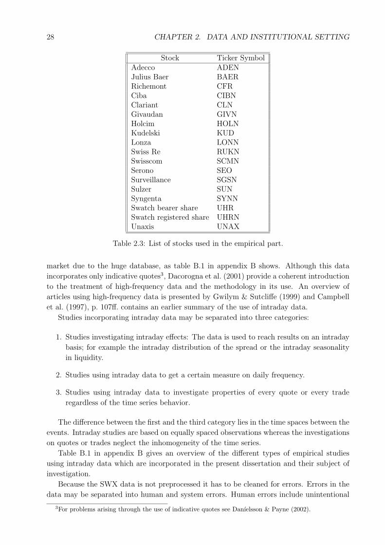
28 CHAPTER 2. DATA AND INSTITUTIONAL SETTING
Stock Ticker SymbolAdecco ADENJulius Baer BAERRichemont CFRCiba CIBNClariant CLNGivaudan GIVNHolcim HOLNKudelski KUDLonza LONNSwiss Re RUKNSwisscom SCMNSerono SEOSurveillance SGSNSulzer SUNSyngenta SYNNSwatch bearer share UHRSwatch registered share UHRNUnaxis UNAX
Table 2.3: List of stocks used in the empirical part.
market due to the huge database, as table B.1 in appendix B shows. Although this data
incorporates only indicative quotes3, Dacorogna et al. (2001) provide a coherent introduction
to the treatment of high-frequency data and the methodology in its use. An overview of
articles using high-frequency data is presented by Gwilym & Sutcliffe (1999) and Campbell
et al. (1997), p. 107ff. contains an earlier summary of the use of intraday data.
Studies incorporating intraday data may be separated into three categories:
1. Studies investigating intraday effects: The data is used to reach results on an intraday
basis; for example the intraday distribution of the spread or the intraday seasonality
in liquidity.
2. Studies using intraday data to get a certain measure on daily frequency.
3. Studies using intraday data to investigate properties of every quote or every trade
regardless of the time series behavior.
The difference between the first and the third category lies in the time spaces between the
events. Intraday studies are based on equally spaced observations whereas the investigations
on quotes or trades neglect the inhomogeneity of the time series.
Table B.1 in appendix B gives an overview of the different types of empirical studies
using intraday data which are incorporated in the present dissertation and their subject of
investigation.
Because the SWX data is not preprocessed it has to be cleaned for errors. Errors in the
data may be separated into human and system errors. Human errors include unintentional
3For problems arising through the use of indicative quotes see Danıelsson & Payne (2002).
2.2. DATA 29
errors, such as typing errors and intentional errors, such as dummy ticks, produced just
for technical testing of the computer system. System errors are caused by failures of the
computer system. In this data cleaning process, negative spreads were sorted out, as well
as negative depths. Furthermore, spreads larger than 10% of the actual stock price were
eliminated.
Bid, ask and transaction prices arrive in the limit order book in an irregular sequence
neither in pairs nor synchronous. Therefore, the original data set is inhomogeneous. A
regular time spacing has to be imposed to make the data mathematically tractable. Over
the inhomogeneous time series a five minute grid was imposed to get homogeneous ones with
a regular spacing. This five minute grid is used for example by Wang (2002) and Andersen &
Bollerslev (1997) and it is narrower than the 15 minutes time space used by Ranaldo (2001)
for the Swiss market and, therefore, more accurate. On the other hand, it leaves the market
participants time to react to the liquidity information provided. The first time space in the
morning lasts from 9.00 until 9.05 a.m. Trading goes on until 5.20 p.m. The closing auction
is left out because the spreads become too large and distort the data series. At the five
minute time interval, one day has 100 data points, yielding for one stock 6500 data points.
There are two interpolation methods that may be used:
• linear interpolation
• previous-tick interpolation
Usually, the difference between the two methods leads to apparently the same results. In
the present dissertation the previous-tick interpolation will be used because it incorporates
only available information at the point of the interpolation, whereas linear interpolation has
to rely on future information.

30 CHAPTER 2. DATA AND INSTITUTIONAL SETTING
Chapter 3
Summary Statistics and Correlations
In this chapter I present the summary statistics and correlations of the 31 liquidity measures.
Correlations among liquidity measures are looked at in a variety of studies, but a complete
overview in literature is missing to date.
The empirical findings to date about co-movement of liquidity measures yield a variety of
results, which are partially contradictive. One of the few stylized facts is that large spreads
are associated with low depth.1
The interrelation of trading volume and spread is ambiguous: In Lee et al. (1993) high
trading volume leads to larger spreads and lower depth, but Chan & Pinder (2000) as
well as Chordia, Roll & Subrahmanyam (2001) document a negative correlation of spreads
and trading volume. Acker et al. (2002) show how trading volume is related to spreads
around earnings announcements, but their study is based on daily closing bid and ask prices
which may not be indicative for liquidity during the day. Additionally, they show in a
regression-based approach that the average spread during the day is, in general, an unbiased
predictor for the closing spread. With the present sample this finding could not be confirmed.
Corwin (1999) describes a negative relationship of the number of trades, trade size and
market capitalization to quoted and effective spreads, but the relationship to quoted depth
is positive. For the Chinese stock market, Yang et al. (2001) report a negative relation
of volume to spread. Karagozoglu (2000) explains the liquidity in the futures market using
trading volume and spread as liquidity measures and the trading volume is negatively related
to the spread.
Kluger & Stephan (1997) document, in an article using daily data, a high rank correlation
for firm size, liquidity ratio, spread, and relative odds ratio. The relative odds ratio was not
presented in the liquidity measures in chapter 1, because it is only able to express liquidity
of one stock relative to another. The co-movement of five liquidity measures is thoroughly
investigated in Chordia et al. (2000).
Commonality in liquidity measures across different stocks is investigated by Hasbrouck
& Seppi (2001). They found, for the log quote slope, 13% of the total variation can be
attributed to the first common factor, but for other liquidity measures this part is smaller
and for the effective spread it does practically not exist. Chordia, Roll & Subrahmanyam
(2001) estimate a “market model” of liquidity: Liquidity of a single stock is explained via
liquidity of the market. Lin et al. (1995) investigate the relation of the components of the
1See e.g. Lee et al. (1993).
31
32 CHAPTER 3. SUMMARY STATISTICS AND CORRELATIONS
spread and trade size and show their intraday variation.
An aspect not considered in this dissertation will be the seasonality in the measures. Daily
seasonality is well documented in the literature (see e.g. Andersen & Bollerslev (1997)) and
leads usually to an U-shape or an L-shape of liquidity. For the FX market also the weekly
patterns are well described.
For the American market, liquidity seems to be highest on Tuesdays and lowest on
Fridays, as Chordia, Roll & Subrahmanyam (2001) state.
At the end of this chapter it should be possible to determine a set of liquidity measures
that are able to capture the dimensions of liquidity presented in section 1.1.
With the averages of the liquidity measures, the stocks are ranked and the most liquid
stock is determined. I also investigate which liquidity measures generate the same rankings
and which ones generate rankings that differ from each other.
3.1 Summary Statistics of the Liquidity Measures
For all liquidity measures mean, median, maximum, minimum, standard deviation, skewness,
kurtosis and the result of the Jarque-Bera test for normality are shown. The test statistic is
calculated as follows:
Jarque−Bera =N
6·(
S2 +(Ku− 3)2
4
)(3.1)
N denotes the number of observations, in our case 6500. S is the skewness and Ku the
kurtosis of the liquidity measure. Since the normal distribution has a skewness of 0 and a
kurtosis of 3, the Jarque-Bera test statistic for a normal distribution becomes zero. Under
the null hypothesis of a normal distribution the test statistic is χ2-distributed with 2 degrees
of freedom. The p-value is the probability that the Jarque-Bera test statistic exceeds the
observed value under the null hypothesis.
3.1.1 Summary Statistics of Adecco
Table 3.1 presents the summary statistics of the 31 liquidity measures for Adecco.
The average number of shares traded in each five minute interval is 8’209 shares which
generates an average turnover of 708’964 CHF. These two liquidity measures have a minimum
of zero and are strongly right-skewed. Average depth is 6’158 shares with a skewness of 66.
There are about 13 trades per five minute interval generated by 31 orders. The average
absolute spread is 0.19 CHF. The relative spreads are around 0.22%. The effective spreads
are a little smaller than half the absolute and relative spreads. The average quote slope is
0.0131. Composite liquidity is very small since dollar depth is much larger than the relative
spread. The liquidity ratio 1 shows that, on average, a turnover of 3.37 mio. CHF has to be
generated to move the price one percent. The liquidity ratio 3 on the other hand indicates
that each trade leads to an absolute price move of 0.07%. Since turnover and number of
trades may fall to zero in a five minute time space, so does the flow ratio. On average, it is
17.4 mio. CHF. The order ratio as a measure of market imbalance is around 0.0324 shares
per CHF. Average composite liquidity is 2.22 · 10−8. The average market impact for a trade
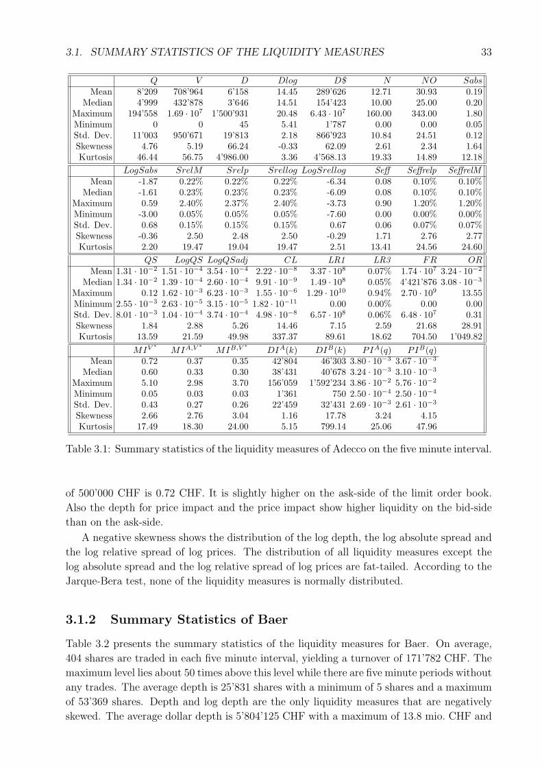
3.1. SUMMARY STATISTICS OF THE LIQUIDITY MEASURES 33
Q V D Dlog D$ N NO SabsMean 8’209 708’964 6’158 14.45 289’626 12.71 30.93 0.19
Median 4’999 432’878 3’646 14.51 154’423 10.00 25.00 0.20Maximum 194’558 1.69 · 107 1’500’931 20.48 6.43 · 107 160.00 343.00 1.80Minimum 0 0 45 5.41 1’787 0.00 0.00 0.05Std. Dev. 11’003 950’671 19’813 2.18 866’923 10.84 24.51 0.12Skewness 4.76 5.19 66.24 -0.33 62.09 2.61 2.34 1.64Kurtosis 46.44 56.75 4’986.00 3.36 4’568.13 19.33 14.89 12.18
LogSabs SrelM Srelp Srellog LogSrellog Seff Seffrelp SeffrelMMean -1.87 0.22% 0.22% 0.22% -6.34 0.08 0.10% 0.10%
Median -1.61 0.23% 0.23% 0.23% -6.09 0.08 0.10% 0.10%Maximum 0.59 2.40% 2.37% 2.40% -3.73 0.90 1.20% 1.20%Minimum -3.00 0.05% 0.05% 0.05% -7.60 0.00 0.00% 0.00%Std. Dev. 0.68 0.15% 0.15% 0.15% 0.67 0.06 0.07% 0.07%Skewness -0.36 2.50 2.48 2.50 -0.29 1.71 2.76 2.77Kurtosis 2.20 19.47 19.04 19.47 2.51 13.41 24.56 24.60
QS LogQS LogQSadj CL LR1 LR3 FR ORMean 1.31 · 10−2 1.51 · 10−4 3.54 · 10−4 2.22 · 10−8 3.37 · 108 0.07% 1.74 · 107 3.24 · 10−2
Median 1.34 · 10−2 1.39 · 10−4 2.60 · 10−4 9.91 · 10−9 1.49 · 108 0.05% 4’421’876 3.08 · 10−3
Maximum 0.12 1.62 · 10−3 6.23 · 10−3 1.55 · 10−6 1.29 · 1010 0.94% 2.70 · 109 13.55Minimum 2.55 · 10−3 2.63 · 10−5 3.15 · 10−5 1.82 · 10−11 0.00 0.00% 0.00 0.00Std. Dev. 8.01 · 10−3 1.04 · 10−4 3.74 · 10−4 4.98 · 10−8 6.57 · 108 0.06% 6.48 · 107 0.31Skewness 1.84 2.88 5.26 14.46 7.15 2.59 21.68 28.91Kurtosis 13.59 21.59 49.98 337.37 89.61 18.62 704.50 1’049.82
MIV ∗ MIA,V ∗ MIB,V ∗ DIA(k) DIB(k) PIA(q) PIB(q)Mean 0.72 0.37 0.35 42’804 46’303 3.80 · 10−3 3.67 · 10−3
Median 0.60 0.33 0.30 38’431 40’678 3.24 · 10−3 3.10 · 10−3
Maximum 5.10 2.98 3.70 156’059 1’592’234 3.86 · 10−2 5.76 · 10−2
Minimum 0.05 0.03 0.03 1’361 750 2.50 · 10−4 2.50 · 10−4
Std. Dev. 0.43 0.27 0.26 22’459 32’431 2.69 · 10−3 2.61 · 10−3
Skewness 2.66 2.76 3.04 1.16 17.78 3.24 4.15Kurtosis 17.49 18.30 24.00 5.15 799.14 25.06 47.96
Table 3.1: Summary statistics of the liquidity measures of Adecco on the five minute interval.
of 500’000 CHF is 0.72 CHF. It is slightly higher on the ask-side of the limit order book.
Also the depth for price impact and the price impact show higher liquidity on the bid-side
than on the ask-side.
A negative skewness shows the distribution of the log depth, the log absolute spread and
the log relative spread of log prices. The distribution of all liquidity measures except the
log absolute spread and the log relative spread of log prices are fat-tailed. According to the
Jarque-Bera test, none of the liquidity measures is normally distributed.
3.1.2 Summary Statistics of Baer
Table 3.2 presents the summary statistics of the liquidity measures for Baer. On average,
404 shares are traded in each five minute interval, yielding a turnover of 171’782 CHF. The
maximum level lies about 50 times above this level while there are five minute periods without
any trades. The average depth is 25’831 shares with a minimum of 5 shares and a maximum
of 53’369 shares. Depth and log depth are the only liquidity measures that are negatively
skewed. The average dollar depth is 5’804’125 CHF with a maximum of 13.8 mio. CHF and
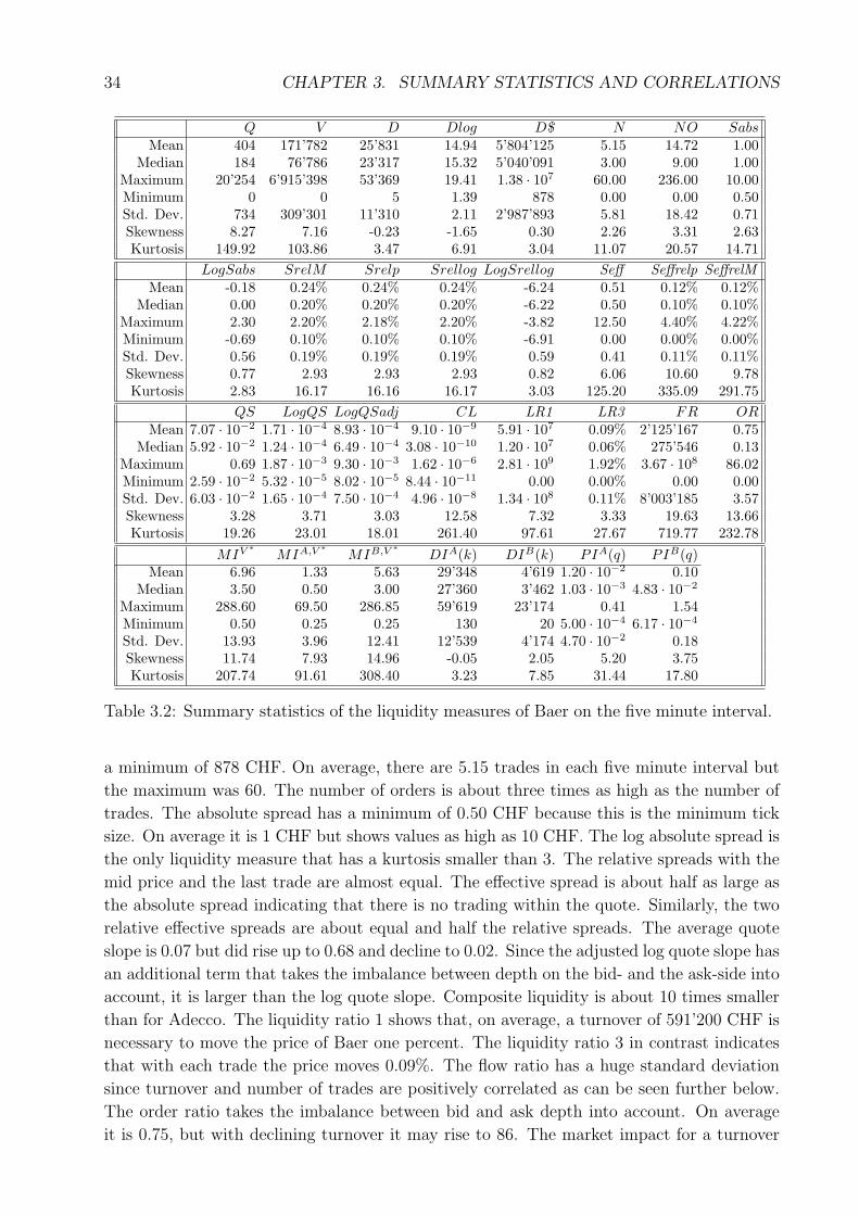
34 CHAPTER 3. SUMMARY STATISTICS AND CORRELATIONS
Q V D Dlog D$ N NO SabsMean 404 171’782 25’831 14.94 5’804’125 5.15 14.72 1.00
Median 184 76’786 23’317 15.32 5’040’091 3.00 9.00 1.00Maximum 20’254 6’915’398 53’369 19.41 1.38 · 107 60.00 236.00 10.00Minimum 0 0 5 1.39 878 0.00 0.00 0.50Std. Dev. 734 309’301 11’310 2.11 2’987’893 5.81 18.42 0.71Skewness 8.27 7.16 -0.23 -1.65 0.30 2.26 3.31 2.63Kurtosis 149.92 103.86 3.47 6.91 3.04 11.07 20.57 14.71
LogSabs SrelM Srelp Srellog LogSrellog Seff Seffrelp SeffrelMMean -0.18 0.24% 0.24% 0.24% -6.24 0.51 0.12% 0.12%
Median 0.00 0.20% 0.20% 0.20% -6.22 0.50 0.10% 0.10%Maximum 2.30 2.20% 2.18% 2.20% -3.82 12.50 4.40% 4.22%Minimum -0.69 0.10% 0.10% 0.10% -6.91 0.00 0.00% 0.00%Std. Dev. 0.56 0.19% 0.19% 0.19% 0.59 0.41 0.11% 0.11%Skewness 0.77 2.93 2.93 2.93 0.82 6.06 10.60 9.78Kurtosis 2.83 16.17 16.16 16.17 3.03 125.20 335.09 291.75
QS LogQS LogQSadj CL LR1 LR3 FR ORMean 7.07 · 10−2 1.71 · 10−4 8.93 · 10−4 9.10 · 10−9 5.91 · 107 0.09% 2’125’167 0.75
Median 5.92 · 10−2 1.24 · 10−4 6.49 · 10−4 3.08 · 10−10 1.20 · 107 0.06% 275’546 0.13Maximum 0.69 1.87 · 10−3 9.30 · 10−3 1.62 · 10−6 2.81 · 109 1.92% 3.67 · 108 86.02Minimum 2.59 · 10−2 5.32 · 10−5 8.02 · 10−5 8.44 · 10−11 0.00 0.00% 0.00 0.00Std. Dev. 6.03 · 10−2 1.65 · 10−4 7.50 · 10−4 4.96 · 10−8 1.34 · 108 0.11% 8’003’185 3.57Skewness 3.28 3.71 3.03 12.58 7.32 3.33 19.63 13.66Kurtosis 19.26 23.01 18.01 261.40 97.61 27.67 719.77 232.78
MIV ∗ MIA,V ∗ MIB,V ∗ DIA(k) DIB(k) PIA(q) PIB(q)Mean 6.96 1.33 5.63 29’348 4’619 1.20 · 10−2 0.10
Median 3.50 0.50 3.00 27’360 3’462 1.03 · 10−3 4.83 · 10−2
Maximum 288.60 69.50 286.85 59’619 23’174 0.41 1.54Minimum 0.50 0.25 0.25 130 20 5.00 · 10−4 6.17 · 10−4
Std. Dev. 13.93 3.96 12.41 12’539 4’174 4.70 · 10−2 0.18Skewness 11.74 7.93 14.96 -0.05 2.05 5.20 3.75Kurtosis 207.74 91.61 308.40 3.23 7.85 31.44 17.80
Table 3.2: Summary statistics of the liquidity measures of Baer on the five minute interval.
a minimum of 878 CHF. On average, there are 5.15 trades in each five minute interval but
the maximum was 60. The number of orders is about three times as high as the number of
trades. The absolute spread has a minimum of 0.50 CHF because this is the minimum tick
size. On average it is 1 CHF but shows values as high as 10 CHF. The log absolute spread is
the only liquidity measure that has a kurtosis smaller than 3. The relative spreads with the
mid price and the last trade are almost equal. The effective spread is about half as large as
the absolute spread indicating that there is no trading within the quote. Similarly, the two
relative effective spreads are about equal and half the relative spreads. The average quote
slope is 0.07 but did rise up to 0.68 and decline to 0.02. Since the adjusted log quote slope has
an additional term that takes the imbalance between depth on the bid- and the ask-side into
account, it is larger than the log quote slope. Composite liquidity is about 10 times smaller
than for Adecco. The liquidity ratio 1 shows that, on average, a turnover of 591’200 CHF is
necessary to move the price of Baer one percent. The liquidity ratio 3 in contrast indicates
that with each trade the price moves 0.09%. The flow ratio has a huge standard deviation
since turnover and number of trades are positively correlated as can be seen further below.
The order ratio takes the imbalance between bid and ask depth into account. On average
it is 0.75, but with declining turnover it may rise to 86. The market impact for a turnover
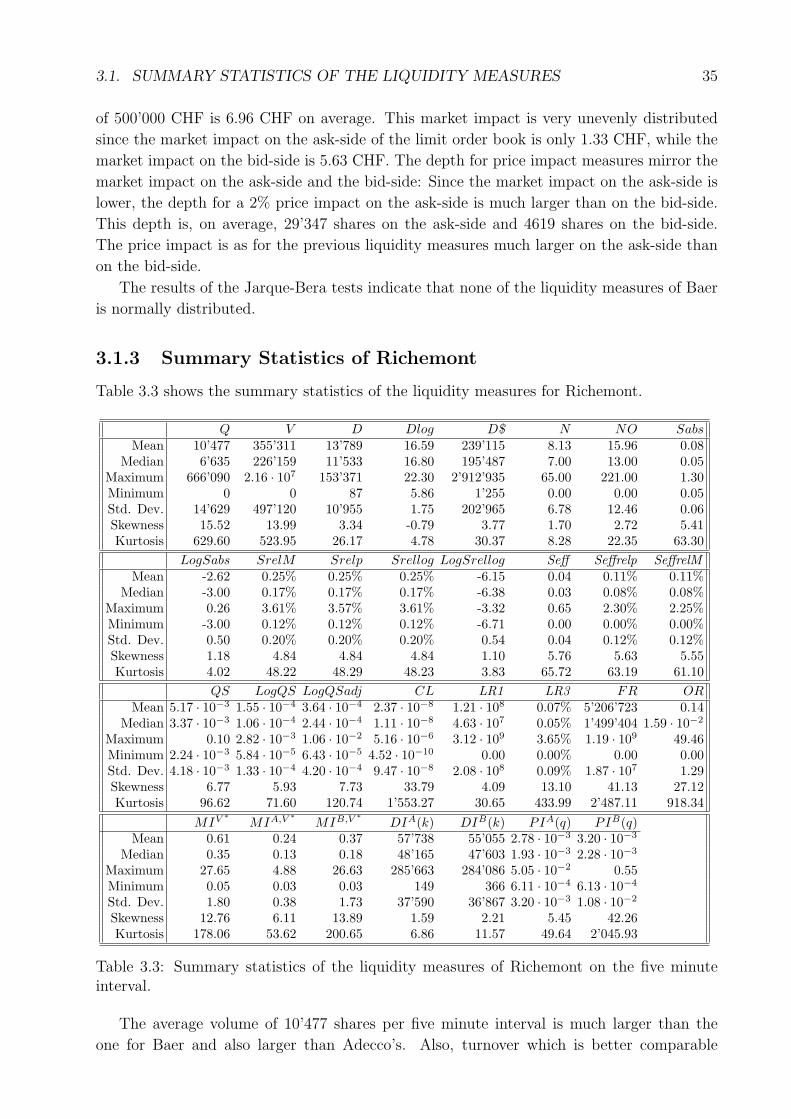
3.1. SUMMARY STATISTICS OF THE LIQUIDITY MEASURES 35
of 500’000 CHF is 6.96 CHF on average. This market impact is very unevenly distributed
since the market impact on the ask-side of the limit order book is only 1.33 CHF, while the
market impact on the bid-side is 5.63 CHF. The depth for price impact measures mirror the
market impact on the ask-side and the bid-side: Since the market impact on the ask-side is
lower, the depth for a 2% price impact on the ask-side is much larger than on the bid-side.
This depth is, on average, 29’347 shares on the ask-side and 4619 shares on the bid-side.
The price impact is as for the previous liquidity measures much larger on the ask-side than
on the bid-side.
The results of the Jarque-Bera tests indicate that none of the liquidity measures of Baer
is normally distributed.
3.1.3 Summary Statistics of Richemont
Table 3.3 shows the summary statistics of the liquidity measures for Richemont.
Q V D Dlog D$ N NO SabsMean 10’477 355’311 13’789 16.59 239’115 8.13 15.96 0.08
Median 6’635 226’159 11’533 16.80 195’487 7.00 13.00 0.05Maximum 666’090 2.16 · 107 153’371 22.30 2’912’935 65.00 221.00 1.30Minimum 0 0 87 5.86 1’255 0.00 0.00 0.05Std. Dev. 14’629 497’120 10’955 1.75 202’965 6.78 12.46 0.06Skewness 15.52 13.99 3.34 -0.79 3.77 1.70 2.72 5.41Kurtosis 629.60 523.95 26.17 4.78 30.37 8.28 22.35 63.30
LogSabs SrelM Srelp Srellog LogSrellog Seff Seffrelp SeffrelMMean -2.62 0.25% 0.25% 0.25% -6.15 0.04 0.11% 0.11%
Median -3.00 0.17% 0.17% 0.17% -6.38 0.03 0.08% 0.08%Maximum 0.26 3.61% 3.57% 3.61% -3.32 0.65 2.30% 2.25%Minimum -3.00 0.12% 0.12% 0.12% -6.71 0.00 0.00% 0.00%Std. Dev. 0.50 0.20% 0.20% 0.20% 0.54 0.04 0.12% 0.12%Skewness 1.18 4.84 4.84 4.84 1.10 5.76 5.63 5.55Kurtosis 4.02 48.22 48.29 48.23 3.83 65.72 63.19 61.10
QS LogQS LogQSadj CL LR1 LR3 FR ORMean 5.17 · 10−3 1.55 · 10−4 3.64 · 10−4 2.37 · 10−8 1.21 · 108 0.07% 5’206’723 0.14
Median 3.37 · 10−3 1.06 · 10−4 2.44 · 10−4 1.11 · 10−8 4.63 · 107 0.05% 1’499’404 1.59 · 10−2
Maximum 0.10 2.82 · 10−3 1.06 · 10−2 5.16 · 10−6 3.12 · 109 3.65% 1.19 · 109 49.46Minimum 2.24 · 10−3 5.84 · 10−5 6.43 · 10−5 4.52 · 10−10 0.00 0.00% 0.00 0.00Std. Dev. 4.18 · 10−3 1.33 · 10−4 4.20 · 10−4 9.47 · 10−8 2.08 · 108 0.09% 1.87 · 107 1.29Skewness 6.77 5.93 7.73 33.79 4.09 13.10 41.13 27.12Kurtosis 96.62 71.60 120.74 1’553.27 30.65 433.99 2’487.11 918.34
MIV ∗ MIA,V ∗ MIB,V ∗ DIA(k) DIB(k) PIA(q) PIB(q)Mean 0.61 0.24 0.37 57’738 55’055 2.78 · 10−3 3.20 · 10−3
Median 0.35 0.13 0.18 48’165 47’603 1.93 · 10−3 2.28 · 10−3
Maximum 27.65 4.88 26.63 285’663 284’086 5.05 · 10−2 0.55Minimum 0.05 0.03 0.03 149 366 6.11 · 10−4 6.13 · 10−4
Std. Dev. 1.80 0.38 1.73 37’590 36’867 3.20 · 10−3 1.08 · 10−2
Skewness 12.76 6.11 13.89 1.59 2.21 5.45 42.26Kurtosis 178.06 53.62 200.65 6.86 11.57 49.64 2’045.93
Table 3.3: Summary statistics of the liquidity measures of Richemont on the five minuteinterval.
The average volume of 10’477 shares per five minute interval is much larger than the
one for Baer and also larger than Adecco’s. Also, turnover which is better comparable
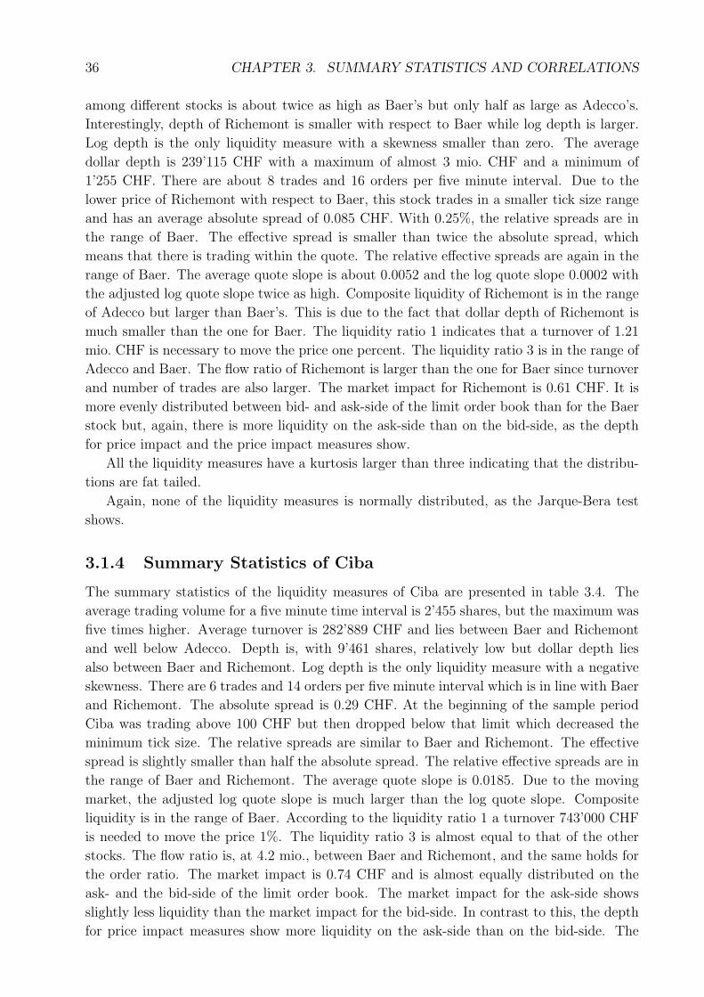
36 CHAPTER 3. SUMMARY STATISTICS AND CORRELATIONS
among different stocks is about twice as high as Baer’s but only half as large as Adecco’s.
Interestingly, depth of Richemont is smaller with respect to Baer while log depth is larger.
Log depth is the only liquidity measure with a skewness smaller than zero. The average
dollar depth is 239’115 CHF with a maximum of almost 3 mio. CHF and a minimum of
1’255 CHF. There are about 8 trades and 16 orders per five minute interval. Due to the
lower price of Richemont with respect to Baer, this stock trades in a smaller tick size range
and has an average absolute spread of 0.085 CHF. With 0.25%, the relative spreads are in
the range of Baer. The effective spread is smaller than twice the absolute spread, which
means that there is trading within the quote. The relative effective spreads are again in the
range of Baer. The average quote slope is about 0.0052 and the log quote slope 0.0002 with
the adjusted log quote slope twice as high. Composite liquidity of Richemont is in the range
of Adecco but larger than Baer’s. This is due to the fact that dollar depth of Richemont is
much smaller than the one for Baer. The liquidity ratio 1 indicates that a turnover of 1.21
mio. CHF is necessary to move the price one percent. The liquidity ratio 3 is in the range of
Adecco and Baer. The flow ratio of Richemont is larger than the one for Baer since turnover
and number of trades are also larger. The market impact for Richemont is 0.61 CHF. It is
more evenly distributed between bid- and ask-side of the limit order book than for the Baer
stock but, again, there is more liquidity on the ask-side than on the bid-side, as the depth
for price impact and the price impact measures show.
All the liquidity measures have a kurtosis larger than three indicating that the distribu-
tions are fat tailed.
Again, none of the liquidity measures is normally distributed, as the Jarque-Bera test
shows.
3.1.4 Summary Statistics of Ciba
The summary statistics of the liquidity measures of Ciba are presented in table 3.4. The
average trading volume for a five minute time interval is 2’455 shares, but the maximum was
five times higher. Average turnover is 282’889 CHF and lies between Baer and Richemont
and well below Adecco. Depth is, with 9’461 shares, relatively low but dollar depth lies
also between Baer and Richemont. Log depth is the only liquidity measure with a negative
skewness. There are 6 trades and 14 orders per five minute interval which is in line with Baer
and Richemont. The absolute spread is 0.29 CHF. At the beginning of the sample period
Ciba was trading above 100 CHF but then dropped below that limit which decreased the
minimum tick size. The relative spreads are similar to Baer and Richemont. The effective
spread is slightly smaller than half the absolute spread. The relative effective spreads are in
the range of Baer and Richemont. The average quote slope is 0.0185. Due to the moving
market, the adjusted log quote slope is much larger than the log quote slope. Composite
liquidity is in the range of Baer. According to the liquidity ratio 1 a turnover 743’000 CHF
is needed to move the price 1%. The liquidity ratio 3 is almost equal to that of the other
stocks. The flow ratio is, at 4.2 mio., between Baer and Richemont, and the same holds for
the order ratio. The market impact is 0.74 CHF and is almost equally distributed on the
ask- and the bid-side of the limit order book. The market impact for the ask-side shows
slightly less liquidity than the market impact for the bid-side. In contrast to this, the depth
for price impact measures show more liquidity on the ask-side than on the bid-side. The
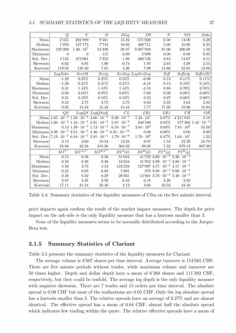
3.1. SUMMARY STATISTICS OF THE LIQUIDITY MEASURES 37
Q V D Dlog D$ N NO SabsMean 2’455 282’889 9’461 15.82 571’026 6.50 14.00 0.29
Median 1’076 127’173 7’745 16.03 460’711 5.00 10.00 0.25Maximum 120’269 1.40 · 107 54’236 20.37 3’367’948 91.00 206.00 1.50Minimum 0 0 115 6.09 5’699 0.00 0.00 0.05Std. Dev. 4’135 472’061 7’352 1.86 460’126 6.84 14.67 0.11Skewness 6.62 6.85 1.90 -0.74 1.95 2.64 3.38 2.55Kurtosis 119.02 128.20 7.81 4.36 7.99 15.86 22.65 13.80
LogSabs SrelM Srelp Srellog LogSrellog Seff Seffrelp SeffrelMMean -1.29 0.25% 0.25% 0.25% -6.06 0.13 0.11% 0.11%
Median -1.39 0.21% 0.21% 0.21% -6.18 0.13 0.10% 0.10%Maximum 0.41 1.44% 1.44% 1.44% -4.24 0.88 0.76% 0.76%Minimum -3.00 0.05% 0.05% 0.05% -7.60 0.00 0.00% 0.00%Std. Dev. 0.31 0.10% 0.10% 0.10% 0.32 0.07 0.06% 0.06%Skewness 0.24 2.75 2.75 2.75 0.83 2.32 2.62 2.62Kurtosis 9.95 15.43 15.43 15.44 7.77 17.30 18.96 18.94
QS LogQS LogQSadj CL LR1 LR3 FR ORMean 1.85 · 10−2 1.58 · 10−4 3.60 · 10−4 9.29 · 10−9 7.43 · 107 0.07% 4’211’835 0.18
Median 1.60 · 10−2 1.34 · 10−4 2.91 · 10−4 5.07 · 10−9 240’100 0.05% 577’363 1.42 · 10−2
Maximum 0.13 1.39 · 10−3 1.13 · 10−2 6.10 · 10−7 3.84 · 109 0.69% 7.85 · 108 53.50Minimum 3.39 · 10−3 3.51 · 10−5 4.46 · 10−5 6.31 · 10−10 0.00 0.00% 0.00 0.00Std. Dev. 7.13 · 10−3 6.84 · 10−5 2.91 · 10−4 1.79 · 10−8 1.78 · 108 0.07% 1.64 · 107 1.22Skewness 3.14 3.60 10.54 12.94 6.87 1.54 22.39 24.78Kurtosis 24.80 32.38 318.30 304.02 89.08 7.32 879.13 887.98
MIV ∗ MIA,V ∗ MIB,V ∗ DIA(k) DIB(k) PIA(q) PIB(q)Mean 0.74 0.38 0.36 51’044 41’570 3.60 · 10−3 3.36 · 10−3
Median 0.50 0.38 0.38 44’644 41’952 2.89 · 10−3 2.80 · 10−3
Maximum 5.50 3.75 4.13 123’258 127’097 4.71 · 10−2 4.17 · 10−2
Minimum 0.25 0.05 0.03 1’601 879 9.89 · 10−4 9.90 · 10−4
Std. Dev. 0.48 0.32 0.28 26’931 14’801 2.78 · 10−3 2.49 · 10−3
Skewness 2.87 3.28 3.50 0.43 0.18 3.26 3.92Kurtosis 17.11 21.24 28.40 2.13 3.60 23.53 34.48
Table 3.4: Summary statistics of the liquidity measures of Ciba on the five minute interval.
price impacts again confirm the result of the market impact measures. The depth for price
impact on the ask-side is the only liquidity measure that has a kurtosis smaller than 3.
None of the liquidity measures seems to be normally distributed according to the Jarque-
Bera test.
3.1.5 Summary Statistics of Clariant
Table 3.5 presents the summary statistics of the liquidity measures for Clariant.
The average volume is 4’607 shares per time interval. Average turnover is 154’065 CHF.
There are five minute periods without trades, while maximum volume and turnover are
50 times higher. Depth and dollar depth have a mean of 6’368 shares and 111’392 CHF,
respectively, but they could be tenfold. The average log depth is the only liquidity measure
with negative skewness. There are 7 trades and 15 orders per time interval. The absolute
spread is 0.09 CHF but most of the realizations are 0.05 CHF. Only the log absolute spread
has a kurtosis smaller than 3. The relative spreads have an average of 0.27% and are almost
identical. The effective spread has a mean of 0.04 CHF, almost half the absolute spread
which indicates few trading within the quote. The relative effective spreads have a mean of
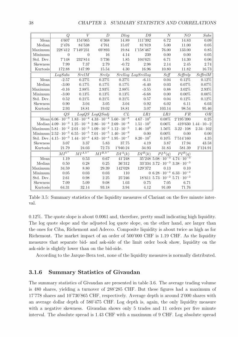
38 CHAPTER 3. SUMMARY STATISTICS AND CORRELATIONS
Q V D Dlog D$ N NO SabsMean 4’607 154’065 6’368 14.89 111’392 6.72 14.83 0.09
Median 2’476 84’538 4’761 15.07 81’819 5.00 11.00 0.05Maximum 228’412 7’149’231 69’893 19.84 1’158’467 76.00 133.00 0.85Minimum 0 0 16 4.14 239 0.00 0.00 0.05Std. Dev. 7’148 232’814 5’736 1.85 104’621 6.71 14.30 0.06Skewness 7.99 7.37 2.79 -0.72 2.98 2.14 2.45 2.74Kurtosis 172.88 147.99 15.54 4.30 16.96 10.80 11.82 16.73
LogSabs SrelM Srelp Srellog LogSrellog Seff Seffrelp SeffrelMMean -2.57 0.27% 0.27% 0.27% -6.11 0.04 0.12% 0.12%
Median -3.00 0.17% 0.17% 0.17% -6.40 0.03 0.07% 0.07%Maximum -0.16 2.88% 2.93% 2.88% -3.55 0.88 3.02% 2.93%Minimum -3.00 0.13% 0.13% 0.13% -6.68 0.00 0.00% 0.00%Std. Dev. 0.52 0.21% 0.21% 0.21% 0.57 0.04 0.12% 0.12%Skewness 0.90 3.04 3.05 3.04 0.92 6.02 6.11 6.03Kurtosis 2.93 18.81 19.02 18.81 3.07 103.14 98.54 95.46
QS LogQS LogQSadj CL LR1 LR3 FR ORMean 6.06 · 10−3 1.83 · 10−4 4.33 · 10−4 5.60 · 10−8 4.67 · 107 0.08% 2’195’390 0.25
Median 4.09 · 10−3 1.25 · 10−4 2.86 · 10−4 2.69 · 10−8 1.51 · 107 0.06% 419’630 1.44 · 10−2Maximum 5.81 · 10−2 2.01 · 10−3 1.09 · 10−2 1.12 · 10−5 1.46 · 109 1.56% 3.22 · 108 2.34 · 102Minimum 2.52 · 10−3 6.55 · 10−5 7.01 · 10−5 1.40 · 10−9 0.00 0.00% 0.00 0.00Std. Dev. 4.15 · 10−3 1.44 · 10−4 4.83 · 10−4 1.95 · 10−7 8.20 · 107 0.10% 7’514’160 4.35Skewness 3.07 3.37 5.83 37.75 4.19 3.87 17.94 43.58Kurtosis 21.79 24.03 72.73 1’940.24 34.93 31.83 581.39 2’124.91
MIV ∗ MIA,V ∗ MIB,V ∗ DIA(k) DIB(k) PIA(q) PIB(q)Mean 1.19 0.53 0.67 41’248 35’248 5.08 · 10−3 4.74 · 10−3
Median 0.50 0.28 0.25 36’312 33’334 3.72 · 10−3 3.38 · 10−3
Maximum 34.59 8.80 29.39 142’028 129’372 0.13 0.10Minimum 0.05 0.03 0.03 110 0 6.28 · 10−4 6.33 · 10−4
Std. Dev. 2.61 0.98 2.25 25’246 18’611 5.73 · 10−3 5.71 · 10−3
Skewness 7.09 5.09 9.08 1.03 0.75 7.05 6.71Kurtosis 64.31 32.14 93.18 3.94 4.12 91.09 71.76
Table 3.5: Summary statistics of the liquidity measures of Clariant on the five minute inter-val.
0.12%. The quote slope is about 0.0061 and, therefore, pretty small indicating high liquidity.
The log quote slope and the adjusted log quote slope, on the other hand, are larger than
the ones for Ciba, Richemont and Adecco. Composite liquidity is about twice as high as for
Richemont. The market impact of an order of 500’000 CHF is 1.19 CHF. As the liquidity
measures that separate bid- and ask-side of the limit order book show, liquidity on the
ask-side is slightly lower than on the bid-side.
According to the Jarque-Bera test, none of the liquidity measures is normally distributed.
3.1.6 Summary Statistics of Givaudan
The summary statistics of Givaudan are presented in table 3.6. The average trading volume
is 480 shares, yielding a turnover of 288’285 CHF. But these figures had a maximum of
17’778 shares and 10’730’865 CHF, respectively. Average depth is around 2’000 shares with
an average dollar depth of 580’475 CHF. Log depth is, again, the only liquidity measure
with a negative skewness. Givaudan shows only 5 trades and 11 orders per five minute
interval. The absolute spread is 1.43 CHF with a maximum of 9 CHF. Log absolute spread
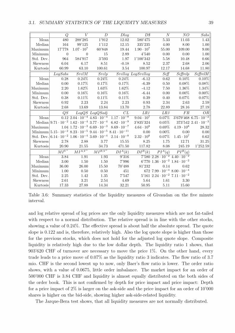
3.1. SUMMARY STATISTICS OF THE LIQUIDITY MEASURES 39
Q V D Dlog D$ N NO SabsMean 480 288’285 1’912 12.02 580’475 5.33 11.03 1.43
Median 164 99’125 1’112 12.15 335’235 4.00 8.00 1.00Maximum 17’778 1.07 · 107 60’848 19.44 1.90 · 107 55.00 109.00 9.00Minimum 0 0 15 2.89 4’540 0.00 0.00 1.00Std. Dev. 964 584’917 3’593 1.97 1’100’342 5.58 10.48 0.66Skewness 6.04 6.17 8.51 -0.18 8.52 2.37 2.68 2.06Kurtosis 60.99 63.10 100.61 3.54 100.97 12.17 14.68 11.80
LogSabs SrelM Srelp Srellog LogSrellog Seff Seffrelp SeffrelMMean 0.28 0.24% 0.24% 0.24% -6.12 0.62 0.10% 0.10%
Median 0.00 0.17% 0.17% 0.17% -6.39 0.50 0.08% 0.08%Maximum 2.20 1.62% 1.63% 1.62% -4.12 7.50 1.36% 1.34%Minimum 0.00 0.16% 0.16% 0.16% -6.44 0.00 0.00% 0.00%Std. Dev. 0.38 0.11% 0.11% 0.11% 0.39 0.40 0.07% 0.07%Skewness 0.92 2.23 2.24 2.23 0.93 2.34 2.63 2.59Kurtosis 2.68 13.69 13.84 13.70 2.78 22.89 28.16 27.19
QS LogQS LogQSadj CL LR1 LR3 FR ORMean 0.12 2.04 · 10−4 4.83 · 10−4 1.17 · 10−8 9.04 · 107 0.07% 3’679’468 6.75 · 10−2
Median 9.71 · 10−2 1.62 · 10−4 3.77 · 10−4 6.82 · 10−9 3’835’324 0.05% 373’542 2.41 · 10−3
Maximum 1.04 1.72 · 10−3 6.69 · 10−3 8.69 · 10−7 4.64 · 109 0.69% 4.19 · 108 28.32Minimum 5.15 · 10−2 8.23 · 10−5 9.44 · 10−5 8.41 · 10−11 0.00 0.00% 0.00 0.00Std. Dev. 6.14 · 10−2 1.06 · 10−4 3.69 · 10−4 2.14 · 10−8 2.32 · 108 0.07% 1.45 · 107 0.62Skewness 2.78 2.88 3.77 15.55 8.25 1.75 12.71 31.25Kurtosis 20.90 21.55 34.73 471.50 117.82 8.08 245.19 1’252.59
MIV ∗ MIA,V ∗ MIB,V ∗ DIA(k) DIB(k) PIA(q) PIB(q)Mean 3.84 1.91 1.93 9’316 7’580 2.28 · 10−2 4.40 · 10−2
Median 3.00 1.50 1.50 7’996 6’770 1.36 · 10−2 1.84 · 10−2
Maximum 36.00 26.00 15.50 70’488 81’232 0.14 0.62Minimum 1.00 0.50 0.50 451 672 7.99 · 10−4 8.00 · 10−4
Std. Dev. 2.25 1.42 1.35 7’547 5’161 2.24 · 10−2 7.11 · 10−2
Skewness 2.61 3.21 2.54 4.69 5.64 1.61 3.30Kurtosis 17.33 27.88 14.34 32.21 50.95 5.11 15.60
Table 3.6: Summary statistics of the liquidity measures of Givaudan on the five minuteinterval.
and log relative spread of log prices are the only liquidity measures which are not fat-tailed
with respect to a normal distribution. The relative spread is in line with the other stocks,
showing a value of 0.24%. The effective spread is about half the absolute spread. The quote
slope is 0.122 and is, therefore, relatively high. Also the log quote slope is higher than those
for the previous stocks, which does not hold for the adjusted log quote slope. Composite
liquidity is relatively high due to the low dollar depth. The liquidity ratio 1 shows, that
903’620 CHF of turnover are necessary to move the price 1%. On the other hand, every
trade leads to a price move of 0.07% as the liquidity ratio 3 indicates. The flow ratio of 3.7
mio. CHF is the second lowest up to now, only Baer’s flow ratio is lower. The order ratio
shows, with a value of 0.0675, little order imbalance. The market impact for an order of
500’000 CHF is 3.84 CHF and liquidity is almost equally distributed on the both sides of
the order book. This is not confirmed by depth for price impact and price impact: Depth
for a price impact of 2% is larger on the ask-side and the price impact for an order of 10’000
shares is higher on the bid-side, showing higher ask-side-related liquidity.
The Jarque-Bera test shows, that all liquidity measures are not normally distributed.
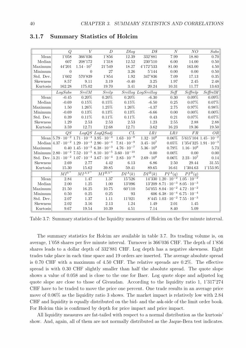
40 CHAPTER 3. SUMMARY STATISTICS AND CORRELATIONS
3.1.7 Summary Statistics of Holcim
Q V D Dlog D$ N NO SabsMean 1’058 366’036 1’856 12.39 332’881 7.99 18.80 0.70
Median 607 208’172 1’318 12.52 230’510 6.00 14.00 0.50Maximum 44’201 1.54 · 107 21’549 18.27 4’172’533 81.00 163.00 4.50Minimum 0 0 27 3.26 5’144 0.00 0.00 0.50Std. Dev. 1’602 570’839 1’854 1.92 347’836 7.09 17.13 0.35Skewness 8.57 9.11 3.19 -0.40 3.25 1.97 2.45 2.48Kurtosis 162.28 175.02 19.70 3.41 20.24 10.31 11.77 13.63
LogSabs SrelM Srelp Srellog LogSrellog Seff Seffrelp SeffrelMMean -0.45 0.20% 0.20% 0.20% -6.30 0.30 0.09% 0.09%
Median -0.69 0.15% 0.15% 0.15% -6.50 0.25 0.07% 0.07%Maximum 1.50 1.26% 1.25% 1.26% -4.37 2.75 0.97% 0.98%Minimum -0.69 0.13% 0.13% 0.13% -6.66 0.00 0.00% 0.00%Std. Dev. 0.39 0.11% 0.11% 0.11% 0.43 0.21 0.07% 0.07%Skewness 1.29 2.53 2.53 2.53 1.23 2.55 2.88 2.88Kurtosis 3.59 12.71 12.68 12.71 3.62 16.23 19.36 19.50
QS LogQS LogQSadj CL LR1 LR3 FR ORMean 5.79 · 10−2 1.71 · 10−4 3.95 · 10−4 1.63 · 10−8 1.32 · 108 0.06% 5’615’104 1.45 · 10−2
Median 4.37 · 10−2 1.29 · 10−4 2.90 · 10−4 7.81 · 10−9 3.45 · 107 0.05% 1’354’325 1.91 · 10−3
Maximum 0.40 1.45 · 10−3 6.38 · 10−3 4.76 · 10−7 5.36 · 109 0.79% 1.16 · 109 5.73Minimum 2.80 · 10−2 7.52 · 10−5 8.10 · 10−5 3.60 · 10−10 0.00 0.00% 0.00 0.00Std. Dev. 3.21 · 10−2 1.07 · 10−4 3.67 · 10−4 2.83 · 10−8 2.69 · 108 0.06% 2.23 · 107 0.14Skewness 2.69 2.77 4.42 6.13 6.86 2.50 29.44 31.55Kurtosis 15.30 15.62 39.85 59.41 89.65 16.61 1’304.63 1’153.95
MIV ∗ MIA,V ∗ MIB,V ∗ DIA(k) DIB(k) PIA(q) PIB(q)Mean 2.84 1.47 1.37 15’526 14’330 1.20 · 10−2 1.05 · 10−2
Median 2.00 1.25 1.00 13’096 13’209 8.71 · 10−3 8.05 · 10−3
Maximum 21.50 16.25 10.75 60’110 54’055 8.04 · 10−2 4.72 · 10−2
Minimum 0.50 0.25 0.25 93 606 6.38 · 10−4 6.75 · 10−4
Std. Dev. 2.07 1.37 1.11 11’021 8’445 1.03 · 10−2 7.55 · 10−3
Skewness 2.02 3.16 2.13 1.24 1.49 2.01 1.45Kurtosis 9.67 19.54 10.39 4.51 7.14 8.40 5.09
Table 3.7: Summary statistics of the liquidity measures of Holcim on the five minute interval.
The summary statistics for Holcim are available in table 3.7. Its trading volume is, on
average, 1’058 shares per five minute interval. Turnover is 366’036 CHF. The depth of 1’856
shares leads to a dollar depth of 332’881 CHF. Log depth has a negative skewness. Eight
trades take place in each time space and 19 orders are inserted. The average absolute spread
is 0.70 CHF with a maximum of 4.50 CHF. The relative spreads are 0.2%. The effective
spread is with 0.30 CHF slightly smaller than half the absolute spread. The quote slope
shows a value of 0.058 and is close to the one for Baer. Log quote slope and adjusted log
quote slope are close to those of Givaudan. According to the liquidity ratio 1, 1’317’274
CHF have to be traded to move the price one percent. One trade results in an average price
move of 0.06% as the liquidity ratio 3 shows. The market impact is relatively low with 2.84
CHF and liquidity is equally distributed on the bid- and the ask-side of the limit order book.
For Holcim this is confirmed by depth for price impact and price impact.
All liquidity measures are fat-tailed with respect to a normal distribution as the kurtosis’
show. And, again, all of them are not normally distributed as the Jaque-Bera test indicates.
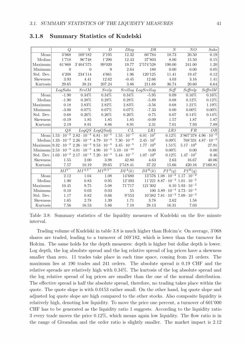
3.1. SUMMARY STATISTICS OF THE LIQUIDITY MEASURES 41
3.1.8 Summary Statistics of Kudelski
Q V D Dlog D$ N NO SabsMean 3’068 169’182 2’195 12.32 60’784 10.73 20.50 0.19
Median 1’718 96’748 1’290 12.43 37’803 8.00 15.50 0.15Maximum 61’868 3’404’575 99’020 19.77 2’574’528 190.00 241.00 1.20Minimum 0 0 9 2.64 180 0.00 0.00 0.05Std. Dev. 4’208 234’114 4’661 1.96 120’125 11.41 19.47 0.12Skewness 3.93 4.41 12.62 -0.45 12.66 4.03 3.16 1.41Kurtosis 29.65 38.24 207.24 3.86 211.68 36.74 20.60 6.64
LogSabs SrelM Srelp Srellog LogSrellog Seff Seffrelp SeffrelMMean -1.90 0.34% 0.34% 0.34% -5.95 0.09 0.16% 0.16%
Median -1.90 0.28% 0.28% 0.28% -5.89 0.08 0.12% 0.12%Maximum 0.18 2.83% 2.82% 2.83% -3.56 0.68 1.21% 1.19%Minimum -3.00 0.07% 0.07% 0.07% -7.33 0.00 0.00% 0.00%Std. Dev. 0.68 0.26% 0.26% 0.26% 0.75 0.07 0.14% 0.14%Skewness -0.19 1.85 1.85 1.85 -0.09 1.57 1.87 1.87Kurtosis 2.19 8.91 8.86 8.91 2.31 7.01 7.93 7.89
QS LogQS LogQSadj CL LR1 LR3 FR ORMean 1.53 · 10−2 2.82 · 10−4 6.81 · 10−4 1.55 · 10−7 6.01 · 107 0.12% 3’867’378 4.96 · 10−2
Median 1.33 · 10−2 2.26 · 10−4 4.79 · 10−4 7.30 · 10−8 2.45 · 107 0.09% 768’331 4.87 · 10−3
Maximum 9.32 · 10−2 2.26 · 10−3 9.53 · 10−3 3.45 · 10−5 1.77 · 109 1.51% 5.17 · 108 27.91Minimum 2.53 · 10−3 4.01 · 10−5 4.90 · 10−5 5.10 · 10−10 0.00 0.00% 0.00 0.00Std. Dev. 1.03 · 10−2 2.17 · 10−4 7.20 · 10−4 5.44 · 10−7 1.07 · 108 0.12% 1.47 · 107 0.46Skewness 1.55 2.00 3.98 42.80 4.63 2.63 16.67 40.06Kurtosis 7.57 10.19 29.65 2’518.41 37.22 15.66 420.16 2’160.81
MIV ∗ MIA,V ∗ MIB,V ∗ DIA(k) DIB(k) PIA(q) PIB(q)Mean 2.12 1.04 1.08 14’680 13’576 1.08 · 10−2 1.17 · 10−2
Median 1.90 0.83 0.95 12’493 11’221 8.87 · 10−3 1.01 · 10−2
Maximum 10.45 9.75 5.08 71’717 121’302 0.10 5.93 · 10−2
Minimum 0.10 0.03 0.03 55 100 3.89 · 10−4 3.73 · 10−4
Std. Dev. 1.17 0.82 0.66 9’553 10’382 7.81 · 10−3 7.09 · 10−3
Skewness 1.65 2.78 1.39 1.71 3.78 2.62 1.58Kurtosis 7.56 16.53 5.86 7.10 28.13 16.31 7.03
Table 3.8: Summary statistics of the liquidity measures of Kudelski on the five minuteinterval.
Trading volume of Kudelski in table 3.8 is much higher than Holcim’s: On average, 3’068
shares are traded, leading to a turnover of 169’182, which is lower than the turnover for
Holcim. The same holds for the depth measures: depth is higher but dollar depth is lower.
Log depth, the log absolute spread and the log relative spread of log prices have a skewness
smaller than zero. 11 trades take place in each time space, coming from 21 orders. The
maximum lies at 190 trades and 241 orders. The absolute spread is 0.19 CHF and the
relative spreads are relatively high with 0.34%. The kurtosis of the log absolute spread and
the log relative spread of log prices are smaller than the one of the normal distribution.
The effective spread is half the absolute spread, therefore, no trading takes place within the
quote. The quote slope is with 0.0153 rather small. On the other hand, log quote slope and
adjusted log quote slope are high compared to the other stocks. Also composite liquidity is
relatively high, denoting low liquidity. To move the price one percent, a turnover of 601’000
CHF has to be generated as the liquidity ratio 1 suggests. According to the liquidity ratio
3 every trade moves the price 0.12%, which means again low liquidity. The flow ratio is in
the range of Givaudan and the order ratio is slightly smaller. The market impact is 2.12
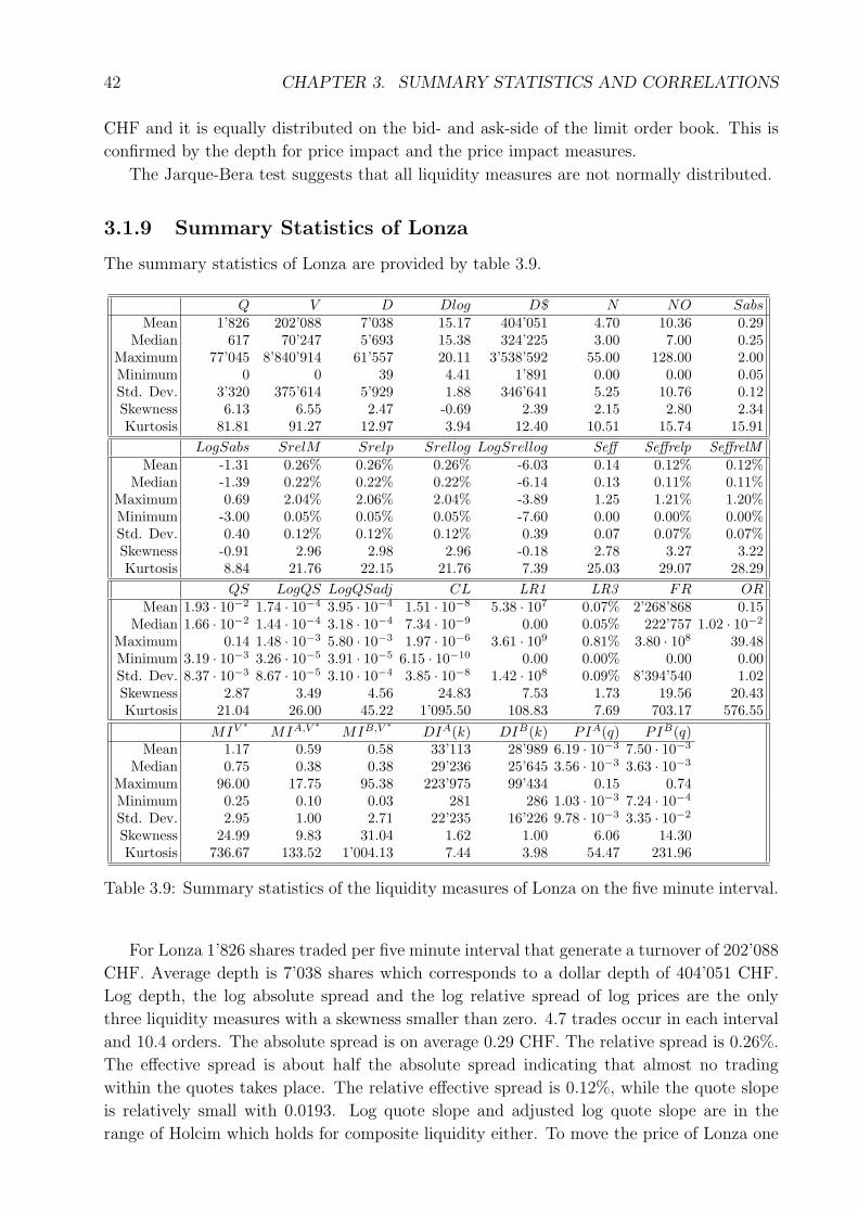
42 CHAPTER 3. SUMMARY STATISTICS AND CORRELATIONS
CHF and it is equally distributed on the bid- and ask-side of the limit order book. This is
confirmed by the depth for price impact and the price impact measures.
The Jarque-Bera test suggests that all liquidity measures are not normally distributed.
3.1.9 Summary Statistics of Lonza
The summary statistics of Lonza are provided by table 3.9.
Q V D Dlog D$ N NO SabsMean 1’826 202’088 7’038 15.17 404’051 4.70 10.36 0.29
Median 617 70’247 5’693 15.38 324’225 3.00 7.00 0.25Maximum 77’045 8’840’914 61’557 20.11 3’538’592 55.00 128.00 2.00Minimum 0 0 39 4.41 1’891 0.00 0.00 0.05Std. Dev. 3’320 375’614 5’929 1.88 346’641 5.25 10.76 0.12Skewness 6.13 6.55 2.47 -0.69 2.39 2.15 2.80 2.34Kurtosis 81.81 91.27 12.97 3.94 12.40 10.51 15.74 15.91
LogSabs SrelM Srelp Srellog LogSrellog Seff Seffrelp SeffrelMMean -1.31 0.26% 0.26% 0.26% -6.03 0.14 0.12% 0.12%
Median -1.39 0.22% 0.22% 0.22% -6.14 0.13 0.11% 0.11%Maximum 0.69 2.04% 2.06% 2.04% -3.89 1.25 1.21% 1.20%Minimum -3.00 0.05% 0.05% 0.05% -7.60 0.00 0.00% 0.00%Std. Dev. 0.40 0.12% 0.12% 0.12% 0.39 0.07 0.07% 0.07%Skewness -0.91 2.96 2.98 2.96 -0.18 2.78 3.27 3.22Kurtosis 8.84 21.76 22.15 21.76 7.39 25.03 29.07 28.29
QS LogQS LogQSadj CL LR1 LR3 FR ORMean 1.93 · 10−2 1.74 · 10−4 3.95 · 10−4 1.51 · 10−8 5.38 · 107 0.07% 2’268’868 0.15
Median 1.66 · 10−2 1.44 · 10−4 3.18 · 10−4 7.34 · 10−9 0.00 0.05% 222’757 1.02 · 10−2
Maximum 0.14 1.48 · 10−3 5.80 · 10−3 1.97 · 10−6 3.61 · 109 0.81% 3.80 · 108 39.48Minimum 3.19 · 10−3 3.26 · 10−5 3.91 · 10−5 6.15 · 10−10 0.00 0.00% 0.00 0.00Std. Dev. 8.37 · 10−3 8.67 · 10−5 3.10 · 10−4 3.85 · 10−8 1.42 · 108 0.09% 8’394’540 1.02Skewness 2.87 3.49 4.56 24.83 7.53 1.73 19.56 20.43Kurtosis 21.04 26.00 45.22 1’095.50 108.83 7.69 703.17 576.55
MIV ∗ MIA,V ∗ MIB,V ∗ DIA(k) DIB(k) PIA(q) PIB(q)Mean 1.17 0.59 0.58 33’113 28’989 6.19 · 10−3 7.50 · 10−3
Median 0.75 0.38 0.38 29’236 25’645 3.56 · 10−3 3.63 · 10−3
Maximum 96.00 17.75 95.38 223’975 99’434 0.15 0.74Minimum 0.25 0.10 0.03 281 286 1.03 · 10−3 7.24 · 10−4
Std. Dev. 2.95 1.00 2.71 22’235 16’226 9.78 · 10−3 3.35 · 10−2
Skewness 24.99 9.83 31.04 1.62 1.00 6.06 14.30Kurtosis 736.67 133.52 1’004.13 7.44 3.98 54.47 231.96
Table 3.9: Summary statistics of the liquidity measures of Lonza on the five minute interval.
For Lonza 1’826 shares traded per five minute interval that generate a turnover of 202’088
CHF. Average depth is 7’038 shares which corresponds to a dollar depth of 404’051 CHF.
Log depth, the log absolute spread and the log relative spread of log prices are the only
three liquidity measures with a skewness smaller than zero. 4.7 trades occur in each interval
and 10.4 orders. The absolute spread is on average 0.29 CHF. The relative spread is 0.26%.
The effective spread is about half the absolute spread indicating that almost no trading
within the quotes takes place. The relative effective spread is 0.12%, while the quote slope
is relatively small with 0.0193. Log quote slope and adjusted log quote slope are in the
range of Holcim which holds for composite liquidity either. To move the price of Lonza one
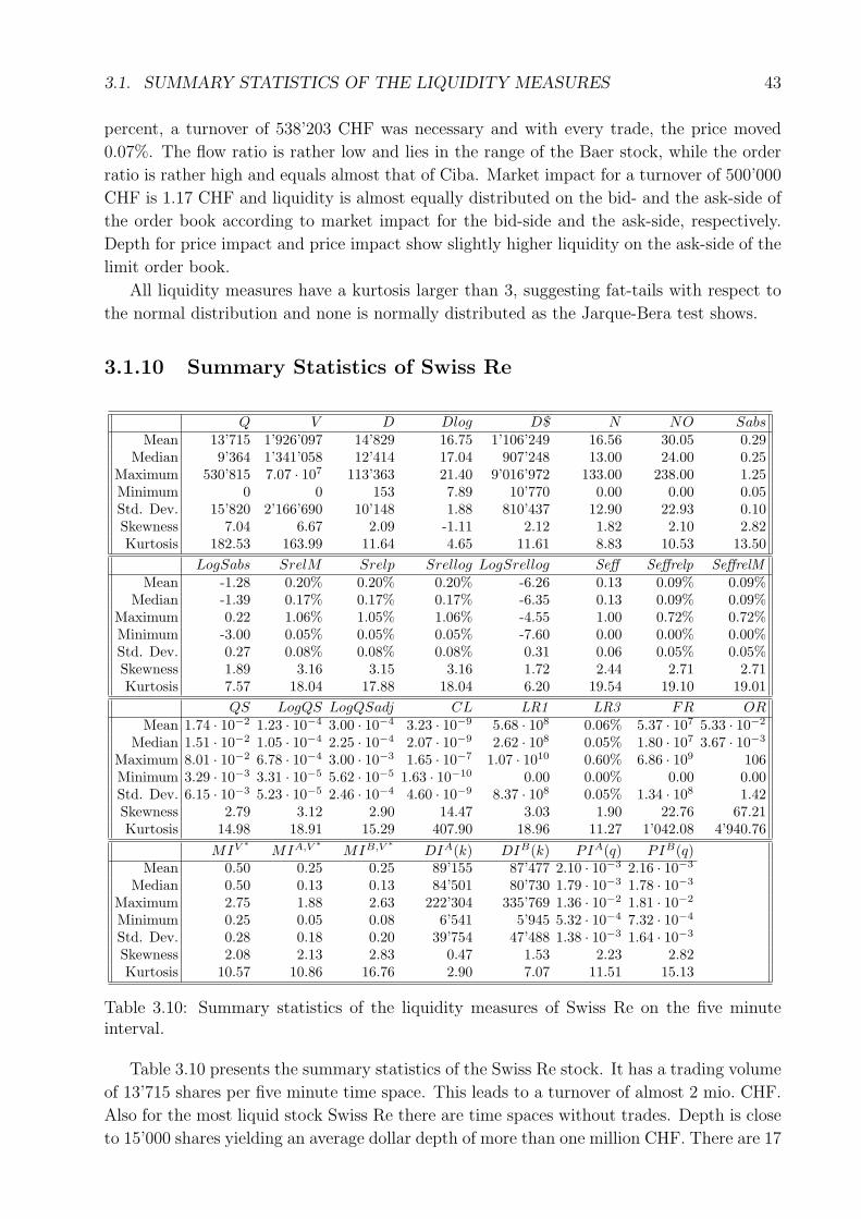
3.1. SUMMARY STATISTICS OF THE LIQUIDITY MEASURES 43
percent, a turnover of 538’203 CHF was necessary and with every trade, the price moved
0.07%. The flow ratio is rather low and lies in the range of the Baer stock, while the order
ratio is rather high and equals almost that of Ciba. Market impact for a turnover of 500’000
CHF is 1.17 CHF and liquidity is almost equally distributed on the bid- and the ask-side of
the order book according to market impact for the bid-side and the ask-side, respectively.
Depth for price impact and price impact show slightly higher liquidity on the ask-side of the
limit order book.
All liquidity measures have a kurtosis larger than 3, suggesting fat-tails with respect to
the normal distribution and none is normally distributed as the Jarque-Bera test shows.
3.1.10 Summary Statistics of Swiss Re
Q V D Dlog D$ N NO SabsMean 13’715 1’926’097 14’829 16.75 1’106’249 16.56 30.05 0.29
Median 9’364 1’341’058 12’414 17.04 907’248 13.00 24.00 0.25Maximum 530’815 7.07 · 107 113’363 21.40 9’016’972 133.00 238.00 1.25Minimum 0 0 153 7.89 10’770 0.00 0.00 0.05Std. Dev. 15’820 2’166’690 10’148 1.88 810’437 12.90 22.93 0.10Skewness 7.04 6.67 2.09 -1.11 2.12 1.82 2.10 2.82Kurtosis 182.53 163.99 11.64 4.65 11.61 8.83 10.53 13.50
LogSabs SrelM Srelp Srellog LogSrellog Seff Seffrelp SeffrelMMean -1.28 0.20% 0.20% 0.20% -6.26 0.13 0.09% 0.09%
Median -1.39 0.17% 0.17% 0.17% -6.35 0.13 0.09% 0.09%Maximum 0.22 1.06% 1.05% 1.06% -4.55 1.00 0.72% 0.72%Minimum -3.00 0.05% 0.05% 0.05% -7.60 0.00 0.00% 0.00%Std. Dev. 0.27 0.08% 0.08% 0.08% 0.31 0.06 0.05% 0.05%Skewness 1.89 3.16 3.15 3.16 1.72 2.44 2.71 2.71Kurtosis 7.57 18.04 17.88 18.04 6.20 19.54 19.10 19.01
QS LogQS LogQSadj CL LR1 LR3 FR ORMean 1.74 · 10−2 1.23 · 10−4 3.00 · 10−4 3.23 · 10−9 5.68 · 108 0.06% 5.37 · 107 5.33 · 10−2
Median 1.51 · 10−2 1.05 · 10−4 2.25 · 10−4 2.07 · 10−9 2.62 · 108 0.05% 1.80 · 107 3.67 · 10−3
Maximum 8.01 · 10−2 6.78 · 10−4 3.00 · 10−3 1.65 · 10−7 1.07 · 1010 0.60% 6.86 · 109 106Minimum 3.29 · 10−3 3.31 · 10−5 5.62 · 10−5 1.63 · 10−10 0.00 0.00% 0.00 0.00Std. Dev. 6.15 · 10−3 5.23 · 10−5 2.46 · 10−4 4.60 · 10−9 8.37 · 108 0.05% 1.34 · 108 1.42Skewness 2.79 3.12 2.90 14.47 3.03 1.90 22.76 67.21Kurtosis 14.98 18.91 15.29 407.90 18.96 11.27 1’042.08 4’940.76
MIV ∗ MIA,V ∗ MIB,V ∗ DIA(k) DIB(k) PIA(q) PIB(q)Mean 0.50 0.25 0.25 89’155 87’477 2.10 · 10−3 2.16 · 10−3
Median 0.50 0.13 0.13 84’501 80’730 1.79 · 10−3 1.78 · 10−3
Maximum 2.75 1.88 2.63 222’304 335’769 1.36 · 10−2 1.81 · 10−2
Minimum 0.25 0.05 0.08 6’541 5’945 5.32 · 10−4 7.32 · 10−4
Std. Dev. 0.28 0.18 0.20 39’754 47’488 1.38 · 10−3 1.64 · 10−3
Skewness 2.08 2.13 2.83 0.47 1.53 2.23 2.82Kurtosis 10.57 10.86 16.76 2.90 7.07 11.51 15.13
Table 3.10: Summary statistics of the liquidity measures of Swiss Re on the five minuteinterval.
Table 3.10 presents the summary statistics of the Swiss Re stock. It has a trading volume
of 13’715 shares per five minute time space. This leads to a turnover of almost 2 mio. CHF.
Also for the most liquid stock Swiss Re there are time spaces without trades. Depth is close
to 15’000 shares yielding an average dollar depth of more than one million CHF. There are 17
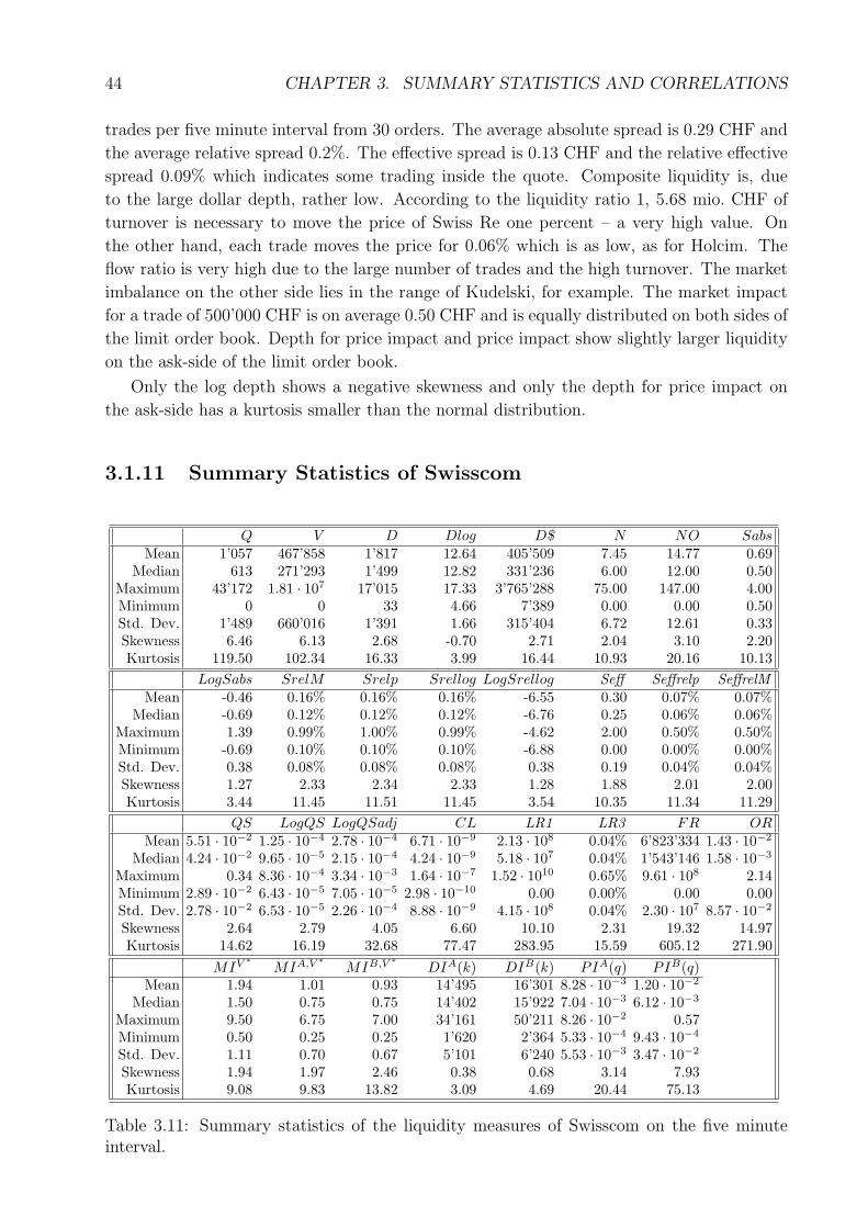
44 CHAPTER 3. SUMMARY STATISTICS AND CORRELATIONS
trades per five minute interval from 30 orders. The average absolute spread is 0.29 CHF and
the average relative spread 0.2%. The effective spread is 0.13 CHF and the relative effective
spread 0.09% which indicates some trading inside the quote. Composite liquidity is, due
to the large dollar depth, rather low. According to the liquidity ratio 1, 5.68 mio. CHF of
turnover is necessary to move the price of Swiss Re one percent – a very high value. On
the other hand, each trade moves the price for 0.06% which is as low, as for Holcim. The
flow ratio is very high due to the large number of trades and the high turnover. The market
imbalance on the other side lies in the range of Kudelski, for example. The market impact
for a trade of 500’000 CHF is on average 0.50 CHF and is equally distributed on both sides of
the limit order book. Depth for price impact and price impact show slightly larger liquidity
on the ask-side of the limit order book.
Only the log depth shows a negative skewness and only the depth for price impact on
the ask-side has a kurtosis smaller than the normal distribution.
3.1.11 Summary Statistics of Swisscom
Q V D Dlog D$ N NO SabsMean 1’057 467’858 1’817 12.64 405’509 7.45 14.77 0.69
Median 613 271’293 1’499 12.82 331’236 6.00 12.00 0.50Maximum 43’172 1.81 · 107 17’015 17.33 3’765’288 75.00 147.00 4.00Minimum 0 0 33 4.66 7’389 0.00 0.00 0.50Std. Dev. 1’489 660’016 1’391 1.66 315’404 6.72 12.61 0.33Skewness 6.46 6.13 2.68 -0.70 2.71 2.04 3.10 2.20Kurtosis 119.50 102.34 16.33 3.99 16.44 10.93 20.16 10.13
LogSabs SrelM Srelp Srellog LogSrellog Seff Seffrelp SeffrelMMean -0.46 0.16% 0.16% 0.16% -6.55 0.30 0.07% 0.07%
Median -0.69 0.12% 0.12% 0.12% -6.76 0.25 0.06% 0.06%Maximum 1.39 0.99% 1.00% 0.99% -4.62 2.00 0.50% 0.50%Minimum -0.69 0.10% 0.10% 0.10% -6.88 0.00 0.00% 0.00%Std. Dev. 0.38 0.08% 0.08% 0.08% 0.38 0.19 0.04% 0.04%Skewness 1.27 2.33 2.34 2.33 1.28 1.88 2.01 2.00Kurtosis 3.44 11.45 11.51 11.45 3.54 10.35 11.34 11.29
QS LogQS LogQSadj CL LR1 LR3 FR ORMean 5.51 · 10−2 1.25 · 10−4 2.78 · 10−4 6.71 · 10−9 2.13 · 108 0.04% 6’823’334 1.43 · 10−2
Median 4.24 · 10−2 9.65 · 10−5 2.15 · 10−4 4.24 · 10−9 5.18 · 107 0.04% 1’543’146 1.58 · 10−3
Maximum 0.34 8.36 · 10−4 3.34 · 10−3 1.64 · 10−7 1.52 · 1010 0.65% 9.61 · 108 2.14Minimum 2.89 · 10−2 6.43 · 10−5 7.05 · 10−5 2.98 · 10−10 0.00 0.00% 0.00 0.00Std. Dev. 2.78 · 10−2 6.53 · 10−5 2.26 · 10−4 8.88 · 10−9 4.15 · 108 0.04% 2.30 · 107 8.57 · 10−2
Skewness 2.64 2.79 4.05 6.60 10.10 2.31 19.32 14.97Kurtosis 14.62 16.19 32.68 77.47 283.95 15.59 605.12 271.90
MIV ∗ MIA,V ∗ MIB,V ∗ DIA(k) DIB(k) PIA(q) PIB(q)Mean 1.94 1.01 0.93 14’495 16’301 8.28 · 10−3 1.20 · 10−2
Median 1.50 0.75 0.75 14’402 15’922 7.04 · 10−3 6.12 · 10−3
Maximum 9.50 6.75 7.00 34’161 50’211 8.26 · 10−2 0.57Minimum 0.50 0.25 0.25 1’620 2’364 5.33 · 10−4 9.43 · 10−4
Std. Dev. 1.11 0.70 0.67 5’101 6’240 5.53 · 10−3 3.47 · 10−2
Skewness 1.94 1.97 2.46 0.38 0.68 3.14 7.93Kurtosis 9.08 9.83 13.82 3.09 4.69 20.44 75.13
Table 3.11: Summary statistics of the liquidity measures of Swisscom on the five minuteinterval.
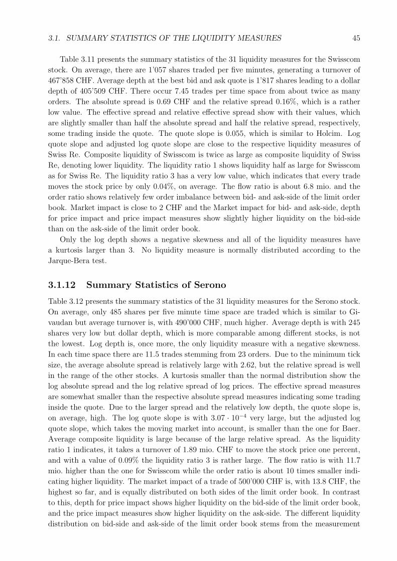
3.1. SUMMARY STATISTICS OF THE LIQUIDITY MEASURES 45
Table 3.11 presents the summary statistics of the 31 liquidity measures for the Swisscom
stock. On average, there are 1’057 shares traded per five minutes, generating a turnover of
467’858 CHF. Average depth at the best bid and ask quote is 1’817 shares leading to a dollar
depth of 405’509 CHF. There occur 7.45 trades per time space from about twice as many
orders. The absolute spread is 0.69 CHF and the relative spread 0.16%, which is a rather
low value. The effective spread and relative effective spread show with their values, which
are slightly smaller than half the absolute spread and half the relative spread, respectively,
some trading inside the quote. The quote slope is 0.055, which is similar to Holcim. Log
quote slope and adjusted log quote slope are close to the respective liquidity measures of
Swiss Re. Composite liquidity of Swisscom is twice as large as composite liquidity of Swiss
Re, denoting lower liquidity. The liquidity ratio 1 shows liquidity half as large for Swisscom
as for Swiss Re. The liquidity ratio 3 has a very low value, which indicates that every trade
moves the stock price by only 0.04%, on average. The flow ratio is about 6.8 mio. and the
order ratio shows relatively few order imbalance between bid- and ask-side of the limit order
book. Market impact is close to 2 CHF and the Market impact for bid- and ask-side, depth
for price impact and price impact measures show slightly higher liquidity on the bid-side
than on the ask-side of the limit order book.
Only the log depth shows a negative skewness and all of the liquidity measures have
a kurtosis larger than 3. No liquidity measure is normally distributed according to the
Jarque-Bera test.
3.1.12 Summary Statistics of Serono
Table 3.12 presents the summary statistics of the 31 liquidity measures for the Serono stock.
On average, only 485 shares per five minute time space are traded which is similar to Gi-
vaudan but average turnover is, with 490’000 CHF, much higher. Average depth is with 245
shares very low but dollar depth, which is more comparable among different stocks, is not
the lowest. Log depth is, once more, the only liquidity measure with a negative skewness.
In each time space there are 11.5 trades stemming from 23 orders. Due to the minimum tick
size, the average absolute spread is relatively large with 2.62, but the relative spread is well
in the range of the other stocks. A kurtosis smaller than the normal distribution show the
log absolute spread and the log relative spread of log prices. The effective spread measures
are somewhat smaller than the respective absolute spread measures indicating some trading
inside the quote. Due to the larger spread and the relatively low depth, the quote slope is,
on average, high. The log quote slope is with 3.07 · 10−4 very large, but the adjusted log
quote slope, which takes the moving market into account, is smaller than the one for Baer.
Average composite liquidity is large because of the large relative spread. As the liquidity
ratio 1 indicates, it takes a turnover of 1.89 mio. CHF to move the stock price one percent,
and with a value of 0.09% the liquidity ratio 3 is rather large. The flow ratio is with 11.7
mio. higher than the one for Swisscom while the order ratio is about 10 times smaller indi-
cating higher liquidity. The market impact of a trade of 500’000 CHF is, with 13.8 CHF, the
highest so far, and is equally distributed on both sides of the limit order book. In contrast
to this, depth for price impact shows higher liquidity on the bid-side of the limit order book,
and the price impact measures show higher liquidity on the ask-side. The different liquidity
distribution on bid-side and ask-side of the limit order book stems from the measurement
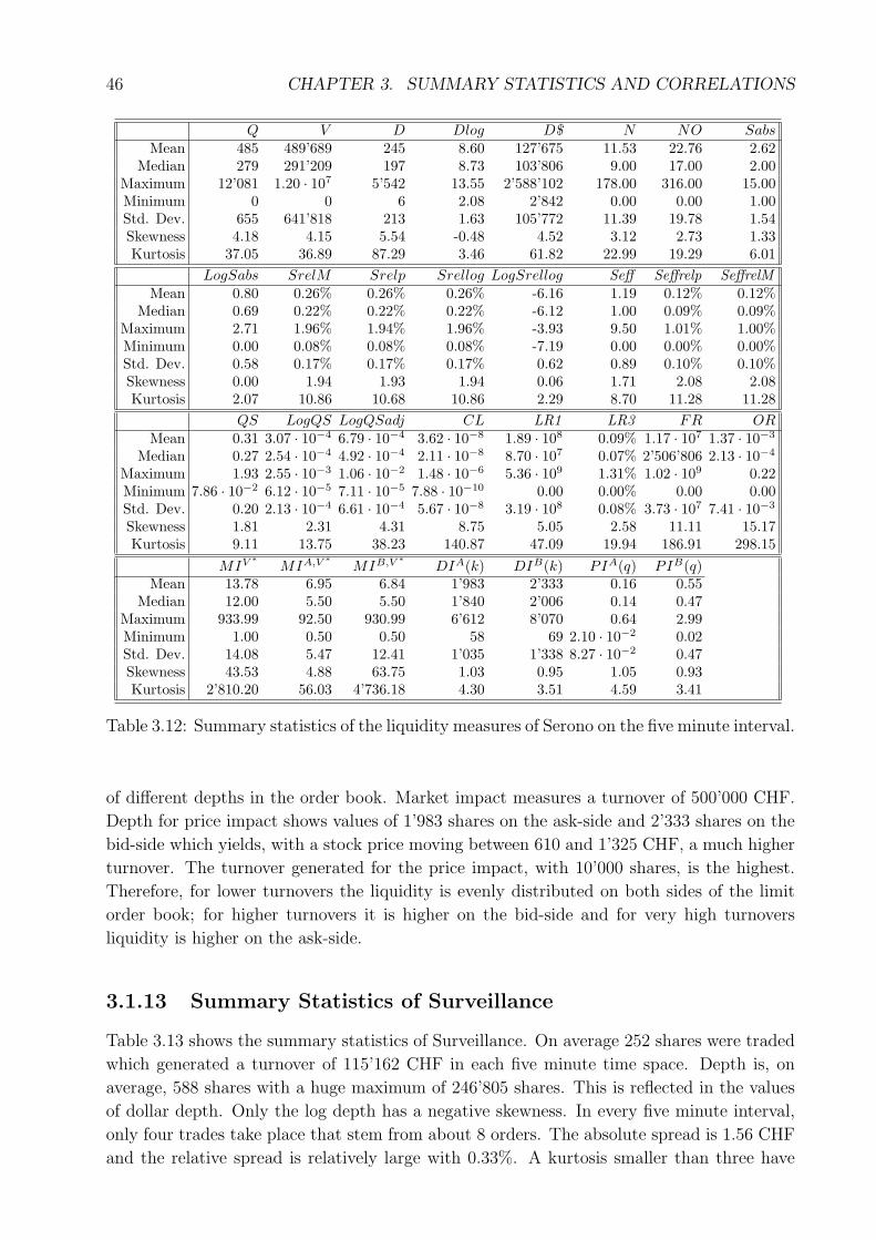
46 CHAPTER 3. SUMMARY STATISTICS AND CORRELATIONS
Q V D Dlog D$ N NO SabsMean 485 489’689 245 8.60 127’675 11.53 22.76 2.62
Median 279 291’209 197 8.73 103’806 9.00 17.00 2.00Maximum 12’081 1.20 · 107 5’542 13.55 2’588’102 178.00 316.00 15.00Minimum 0 0 6 2.08 2’842 0.00 0.00 1.00Std. Dev. 655 641’818 213 1.63 105’772 11.39 19.78 1.54Skewness 4.18 4.15 5.54 -0.48 4.52 3.12 2.73 1.33Kurtosis 37.05 36.89 87.29 3.46 61.82 22.99 19.29 6.01
LogSabs SrelM Srelp Srellog LogSrellog Seff Seffrelp SeffrelMMean 0.80 0.26% 0.26% 0.26% -6.16 1.19 0.12% 0.12%
Median 0.69 0.22% 0.22% 0.22% -6.12 1.00 0.09% 0.09%Maximum 2.71 1.96% 1.94% 1.96% -3.93 9.50 1.01% 1.00%Minimum 0.00 0.08% 0.08% 0.08% -7.19 0.00 0.00% 0.00%Std. Dev. 0.58 0.17% 0.17% 0.17% 0.62 0.89 0.10% 0.10%Skewness 0.00 1.94 1.93 1.94 0.06 1.71 2.08 2.08Kurtosis 2.07 10.86 10.68 10.86 2.29 8.70 11.28 11.28
QS LogQS LogQSadj CL LR1 LR3 FR ORMean 0.31 3.07 · 10−4 6.79 · 10−4 3.62 · 10−8 1.89 · 108 0.09% 1.17 · 107 1.37 · 10−3
Median 0.27 2.54 · 10−4 4.92 · 10−4 2.11 · 10−8 8.70 · 107 0.07% 2’506’806 2.13 · 10−4
Maximum 1.93 2.55 · 10−3 1.06 · 10−2 1.48 · 10−6 5.36 · 109 1.31% 1.02 · 109 0.22Minimum 7.86 · 10−2 6.12 · 10−5 7.11 · 10−5 7.88 · 10−10 0.00 0.00% 0.00 0.00Std. Dev. 0.20 2.13 · 10−4 6.61 · 10−4 5.67 · 10−8 3.19 · 108 0.08% 3.73 · 107 7.41 · 10−3
Skewness 1.81 2.31 4.31 8.75 5.05 2.58 11.11 15.17Kurtosis 9.11 13.75 38.23 140.87 47.09 19.94 186.91 298.15
MIV ∗ MIA,V ∗ MIB,V ∗ DIA(k) DIB(k) PIA(q) PIB(q)Mean 13.78 6.95 6.84 1’983 2’333 0.16 0.55
Median 12.00 5.50 5.50 1’840 2’006 0.14 0.47Maximum 933.99 92.50 930.99 6’612 8’070 0.64 2.99Minimum 1.00 0.50 0.50 58 69 2.10 · 10−2 0.02Std. Dev. 14.08 5.47 12.41 1’035 1’338 8.27 · 10−2 0.47Skewness 43.53 4.88 63.75 1.03 0.95 1.05 0.93Kurtosis 2’810.20 56.03 4’736.18 4.30 3.51 4.59 3.41
Table 3.12: Summary statistics of the liquidity measures of Serono on the five minute interval.
of different depths in the order book. Market impact measures a turnover of 500’000 CHF.
Depth for price impact shows values of 1’983 shares on the ask-side and 2’333 shares on the
bid-side which yields, with a stock price moving between 610 and 1’325 CHF, a much higher
turnover. The turnover generated for the price impact, with 10’000 shares, is the highest.
Therefore, for lower turnovers the liquidity is evenly distributed on both sides of the limit
order book; for higher turnovers it is higher on the bid-side and for very high turnovers
liquidity is higher on the ask-side.
3.1.13 Summary Statistics of Surveillance
Table 3.13 shows the summary statistics of Surveillance. On average 252 shares were traded
which generated a turnover of 115’162 CHF in each five minute time space. Depth is, on
average, 588 shares with a huge maximum of 246’805 shares. This is reflected in the values
of dollar depth. Only the log depth has a negative skewness. In every five minute interval,
only four trades take place that stem from about 8 orders. The absolute spread is 1.56 CHF
and the relative spread is relatively large with 0.33%. A kurtosis smaller than three have
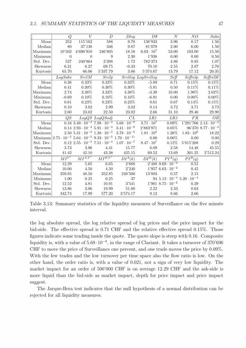
3.1. SUMMARY STATISTICS OF THE LIQUIDITY MEASURES 47
Q V D Dlog D$ N NO SabsMean 252 115’162 588 9.78 138’933 3.96 8.17 1.56
Median 80 37’138 346 9.87 81’079 2.00 6.00 1.50Maximum 10’502 4’696’910 246’805 18.16 6.03 · 107 53.00 103.00 15.50Minimum 0 0 9 2.30 1’938 0.00 0.00 0.50Std. Dev. 527 240’864 3’208 1.72 782’373 4.86 8.85 1.07Skewness 6.21 6.27 69.75 -0.33 70.10 2.55 2.87 2.76Kurtosis 65.70 66.06 5’337.79 3.86 5’374.67 13.79 17.12 20.35
LogSabs SrelM Srelp Srellog LogSrellog Seff Seffrelp SeffrelMMean 0.26 0.33% 0.33% 0.33% -5.89 0.71 0.15% 0.15%
Median 0.41 0.30% 0.30% 0.30% -5.81 0.50 0.11% 0.11%Maximum 2.74 3.38% 3.33% 3.38% -3.39 10.00 1.98% 2.02%Minimum -0.69 0.10% 0.10% 0.10% -6.91 0.00 0.00% 0.00%Std. Dev. 0.61 0.23% 0.23% 0.23% 0.61 0.67 0.14% 0.15%Skewness 0.10 3.02 2.99 3.02 0.14 3.72 3.71 3.73Kurtosis 2.60 23.02 22.50 23.02 2.66 31.10 29.46 29.90
QS LogQS LogQSadj CL LR1 LR3 FR ORMean 0.16 3.49 · 10−4 7.98 · 10−4 5.68 · 10−8 3.71 · 107 0.09% 1’291’766 2.13 · 10−2
Median 0.14 2.93 · 10−4 5.91 · 10−4 3.41 · 10−8 2’883’971 0.05% 96’370 9.77 · 10−4
Maximum 2.50 5.31 · 10−3 1.38 · 10−2 3.78 · 10−6 1.81 · 109 1.26% 1.83 · 108 18.22Minimum 2.75 · 10−2 5.64 · 10−5 9.33 · 10−5 1.70 · 10−11 0.00 0.00% 0.00 0.00Std. Dev. 0.12 2.55 · 10−4 7.51 · 10−4 1.07 · 10−7 8.47 · 107 0.12% 5’815’208 0.29Skewness 3.73 3.96 4.41 15.77 6.09 2.58 14.48 45.55Kurtosis 41.42 42.10 43.38 425.15 69.52 13.69 301.25 2’512.24
MIV ∗ MIA,V ∗ MIB,V ∗ DIA(k) DIB(k) PIA(q) PIB(q)Mean 12.29 5.65 6.65 2’688 2’488 9.69 · 10−2 0.51
Median 10.00 4.50 4.50 2’240 1’957 6.63 · 10−2 0.45Maximum 359.85 48.50 352.85 248’500 13’803 0.57 2.15Minimum 1.00 0.25 0.25 37 94 5.12 · 10−4 5.20 · 10−4
Std. Dev. 12.52 4.81 10.91 3’541 1’901 8.75 · 10−2 0.39Skewness 13.86 3.06 19.99 51.80 2.22 2.33 0.63Kurtosis 342.74 17.99 577.20 3’574.17 9.12 8.66 2.66
Table 3.13: Summary statistics of the liquidity measures of Surveillance on the five minuteinterval.
the log absolute spread, the log relative spread of log prices and the price impact for the
bid-side. The effective spread is 0.71 CHF and the relative effective spread 0.15%. Those
figures indicate some trading inside the quote. The quote slope is steep with 0.16. Composite
liquidity is, with a value of 5.68 ·10−8, in the range of Clariant. It takes a turnover of 370’696
CHF to move the price of Surveillance one percent, and one trade moves the price by 0.09%.
With the few trades and the low turnover per time space also the flow ratio is low. On the
other hand, the order ratio is, with a value of 0.021, not a sign of very low liquidity. The
market impact for an order of 500’000 CHF is on average 12.29 CHF and the ask-side is
more liquid than the bid-side as market impact, depth for price impact and price impact
suggest.
The Jarque-Bera test indicates that the null hypothesis of a normal distribution can be
rejected for all liquidity measures.
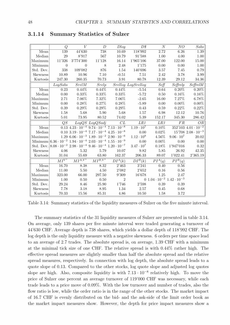
48 CHAPTER 3. SUMMARY STATISTICS AND CORRELATIONS
3.1.14 Summary Statistics of Sulzer
Q V D Dlog D$ N NO SabsMean 139 44’630 738 10.69 118’992 2.72 6.26 1.39
Median 29 8’917 567 10.79 91’588 1.00 4.00 1.00Maximum 11’326 3’774’300 11’128 16.14 1’965’106 37.00 122.00 15.00Minimum 0 0 8 2.48 1’175 0.00 0.00 1.00Std. Dev. 338 109’082 876 1.54 140’696 3.57 7.45 0.79Skewness 10.89 10.96 7.10 -0.51 7.51 2.42 3.78 3.99Kurtosis 247.30 260.35 70.73 3.91 80.78 12.39 29.12 34.36
LogSabs SrelM Srelp Srellog LogSrellog Seff Seffrelp SeffrelMMean 0.23 0.44% 0.44% 0.44% -5.54 0.64 0.20% 0.20%
Median 0.00 0.33% 0.33% 0.33% -5.72 0.50 0.16% 0.16%Maximum 2.71 7.06% 7.32% 7.06% -2.65 16.00 7.27% 6.78%Minimum 0.00 0.28% 0.27% 0.28% -5.89 0.00 0.00% 0.00%Std. Dev. 0.39 0.29% 0.29% 0.29% 0.43 0.59 0.22% 0.22%Skewness 1.58 5.68 5.90 5.68 1.57 6.98 12.12 10.76Kurtosis 5.01 73.95 80.52 74.02 5.39 152.17 345.30 286.42
QS LogQS LogQSadj CL LR1 LR3 FR ORMean 0.13 4.23 · 10−4 9.74 · 10−4 7.13 · 10−8 1.19 · 107 0.10% 352’103 4.01 · 10−2
Median 0.10 3.19 · 10−4 7.17 · 10−4 4.25 · 10−8 0.00 0.02% 15’708 2.08 · 10−3
Maximum 1.29 6.06 · 10−3 1.89 · 10−2 2.90 · 10−6 1.12 · 109 4.56% 9.06 · 107 20.02Minimum 6.36 · 10−2 1.94 · 10−4 2.03 · 10−4 1.55 · 10−9 0.00 0.00% 0.00 0.00Std. Dev. 8.08 · 10−2 2.98 · 10−4 9.46 · 10−4 1.20 · 10−7 3.47 · 107 0.18% 1’947’016 0.32Skewness 4.06 5.32 5.79 10.07 9.82 5.85 26.92 42.35Kurtosis 31.04 55.69 63.80 162.37 206.33 89.07 1’022.41 2’365.19
MIV ∗ MIA,V ∗ MIB,V ∗ DIA(k) DIB(k) PIA(q) PIB(q)Mean 16.70 8.38 8.32 2’463 3’241 0.40 0.56
Median 11.00 5.50 4.50 2’082 2’652 0.16 0.56Maximum 323.00 66.00 297.50 9’309 16’678 1.25 2.47Minimum 1.00 0.50 0.50 2 0 1.04 · 10−2 1.42 · 10−3
Std. Dev. 29.24 8.46 25.90 1’746 2’598 0.39 0.39Skewness 7.78 3.18 8.95 1.34 2.57 0.45 0.68Kurtosis 70.33 15.56 85.31 4.86 10.50 1.58 3.72
Table 3.14: Summary statistics of the liquidity measures of Sulzer on the five minute interval.
The summary statistics of the 31 liquidity measures of Sulzer are presented in table 3.14.
On average, only 139 shares per five minute interval were traded generating a turnover of
44’630 CHF. Average depth is 738 shares, which yields a dollar depth of 118’992 CHF. The
log depth is the only liquidity measure with a negative skewness. 6 orders per time space lead
to an average of 2.7 trades. The absolute spread is, on average, 1.39 CHF with a minimum
at the minimal tick size of one CHF. The relative spread is with 0.44% rather high. The
effective spread measures are slightly smaller than half the absolute spread and the relative
spread measures, respectively. In connection with log depth, the absolute spread leads to a
quote slope of 0.13. Compared to the other stocks, log quote slope and adjusted log quotes
slope are high. Also, composite liquidity is with 7.13 · 10−8 relatively high. To move the
price of Sulzer one percent an average turnover of 119’000 CHF was necessary, while each
trade leads to a price move of 0.09%. With the low turnover and number of trades, also the
flow ratio is low, while the order ratio is in the range of the other stocks. The market impact
of 16.7 CHF is evenly distributed on the bid- and the ask-side of the limit order book as
the market impact measures show. However, the depth for price impact measures show a
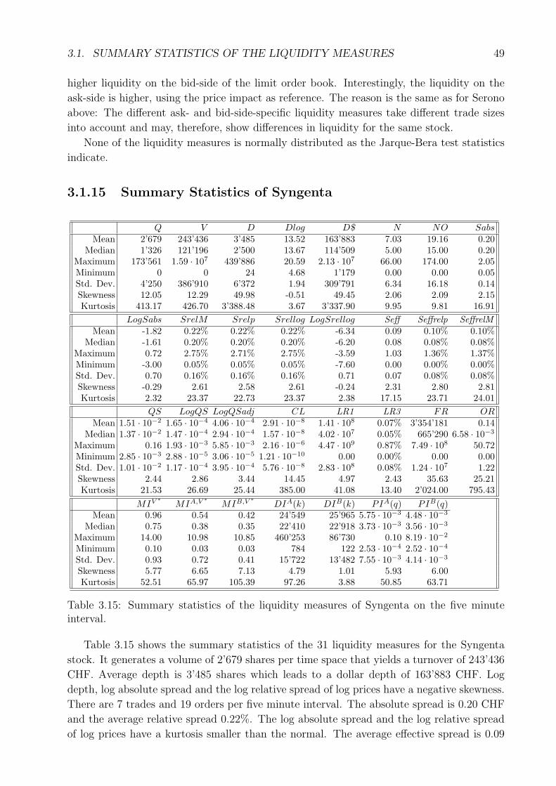
3.1. SUMMARY STATISTICS OF THE LIQUIDITY MEASURES 49
higher liquidity on the bid-side of the limit order book. Interestingly, the liquidity on the
ask-side is higher, using the price impact as reference. The reason is the same as for Serono
above: The different ask- and bid-side-specific liquidity measures take different trade sizes
into account and may, therefore, show differences in liquidity for the same stock.
None of the liquidity measures is normally distributed as the Jarque-Bera test statistics
indicate.
3.1.15 Summary Statistics of Syngenta
Q V D Dlog D$ N NO SabsMean 2’679 243’436 3’485 13.52 163’883 7.03 19.16 0.20
Median 1’326 121’196 2’500 13.67 114’509 5.00 15.00 0.20Maximum 173’561 1.59 · 107 439’886 20.59 2.13 · 107 66.00 174.00 2.05Minimum 0 0 24 4.68 1’179 0.00 0.00 0.05Std. Dev. 4’250 386’910 6’372 1.94 309’791 6.34 16.18 0.14Skewness 12.05 12.29 49.98 -0.51 49.45 2.06 2.09 2.15Kurtosis 413.17 426.70 3’388.48 3.67 3’337.90 9.95 9.81 16.91
LogSabs SrelM Srelp Srellog LogSrellog Seff Seffrelp SeffrelMMean -1.82 0.22% 0.22% 0.22% -6.34 0.09 0.10% 0.10%
Median -1.61 0.20% 0.20% 0.20% -6.20 0.08 0.08% 0.08%Maximum 0.72 2.75% 2.71% 2.75% -3.59 1.03 1.36% 1.37%Minimum -3.00 0.05% 0.05% 0.05% -7.60 0.00 0.00% 0.00%Std. Dev. 0.70 0.16% 0.16% 0.16% 0.71 0.07 0.08% 0.08%Skewness -0.29 2.61 2.58 2.61 -0.24 2.31 2.80 2.81Kurtosis 2.32 23.37 22.73 23.37 2.38 17.15 23.71 24.01
QS LogQS LogQSadj CL LR1 LR3 FR ORMean 1.51 · 10−2 1.65 · 10−4 4.06 · 10−4 2.91 · 10−8 1.41 · 108 0.07% 3’354’181 0.14
Median 1.37 · 10−2 1.47 · 10−4 2.94 · 10−4 1.57 · 10−8 4.02 · 107 0.05% 665’290 6.58 · 10−3
Maximum 0.16 1.93 · 10−3 5.85 · 10−3 2.16 · 10−6 4.47 · 109 0.87% 7.49 · 108 50.72Minimum 2.85 · 10−3 2.88 · 10−5 3.06 · 10−5 1.21 · 10−10 0.00 0.00% 0.00 0.00Std. Dev. 1.01 · 10−2 1.17 · 10−4 3.95 · 10−4 5.76 · 10−8 2.83 · 108 0.08% 1.24 · 107 1.22Skewness 2.44 2.86 3.44 14.45 4.97 2.43 35.63 25.21Kurtosis 21.53 26.69 25.44 385.00 41.08 13.40 2’024.00 795.43
MIV ∗ MIA,V ∗ MIB,V ∗ DIA(k) DIB(k) PIA(q) PIB(q)Mean 0.96 0.54 0.42 24’549 25’965 5.75 · 10−3 4.48 · 10−3
Median 0.75 0.38 0.35 22’410 22’918 3.73 · 10−3 3.56 · 10−3
Maximum 14.00 10.98 10.85 460’253 86’730 0.10 8.19 · 10−2
Minimum 0.10 0.03 0.03 784 122 2.53 · 10−4 2.52 · 10−4
Std. Dev. 0.93 0.72 0.41 15’722 13’482 7.55 · 10−3 4.14 · 10−3
Skewness 5.77 6.65 7.13 4.79 1.01 5.93 6.00Kurtosis 52.51 65.97 105.39 97.26 3.88 50.85 63.71
Table 3.15: Summary statistics of the liquidity measures of Syngenta on the five minuteinterval.
Table 3.15 shows the summary statistics of the 31 liquidity measures for the Syngenta
stock. It generates a volume of 2’679 shares per time space that yields a turnover of 243’436
CHF. Average depth is 3’485 shares which leads to a dollar depth of 163’883 CHF. Log
depth, log absolute spread and the log relative spread of log prices have a negative skewness.
There are 7 trades and 19 orders per five minute interval. The absolute spread is 0.20 CHF
and the average relative spread 0.22%. The log absolute spread and the log relative spread
of log prices have a kurtosis smaller than the normal. The average effective spread is 0.09
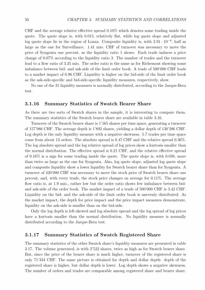
50 CHAPTER 3. SUMMARY STATISTICS AND CORRELATIONS
CHF and the average relative effective spread 0.10% which denotes some trading inside the
quote. The quote slope is, with 0.015, relatively flat, while log quote slope and adjusted
log quote slope lie in the region of Lonza. Composite liquidity is, with 2.91 · 10−8, half as
large as the one for Surveillance. 1.41 mio. CHF of turnover was necessary to move the
price of Syngenta one percent, as the liquidity ratio 1 shows. Each trade induces a price
change of 0.07% according to the liquidity ratio 3. The number of trades and the turnover
lead to a flow ratio of 3.35 mio. The order ratio is the same as for Richemont showing some
imbalance between bid- and ask-side of the limit order book. A trade of 500’000 CHF leads
to a market impact of 0.96 CHF. Liquidity is higher on the bid-side of the limit order book
as the ask-side-specific and bid-side-specific liquidity measures, respectively, show.
No one of the 31 liquidity measures is normally distributed, according to the Jarque-Bera
test.
3.1.16 Summary Statistics of Swatch Bearer Share
As there are two sorts of Swatch shares in the sample, it is interesting to compare them.
The summary statistics of the Swatch bearer share are available in table 3.16.
Turnover of the Swatch bearer share is 1’165 shares per time space, generating a turnover
of 157’986 CHF. The average depth is 1’892 shares, yielding a dollar depth of 130’286 CHF.
Log depth is the only liquidity measure with a negative skewness. 5.7 trades per time space
come from about 13 orders. The absolute spread is 0.47 CHF and the relative spread 0.36%.
The log absolute spread and the log relative spread of log prices show a kurtosis smaller than
the normal distribution. The effective spread is 0.21 CHF, and the relative effective spread
of 0.16% is a sign for some trading inside the quote. The quote slope is, with 0.038, more
than twice as large as the one for Syngenta. Also, log quote slope, adjusted log quote slope
and composite liquidity show a lower liquidity for Swatch bearer share than for Syngenta. A
turnover of 420’000 CHF was necessary to move the stock price of Swatch bearer share one
percent, and, with every trade, the stock price changes on average for 0.11%. The average
flow ratio is, at 1.9 mio., rather low but the order ratio shows few imbalance between bid-
and ask-side of the order book. The market impact of a trade of 500’000 CHF is 3.42 CHF.
Liquidity on the bid- and the ask-side of the limit order book is unevenly distributed: As
the market impact, the depth for price impact and the price impact measures demonstrate,
liquidity on the ask-side is smaller than on the bid-side.
Only the log depth is left-skewed and log absolute spread and the log spread of log prices
have a kurtosis smaller than the normal distribution. No liquidity measure is normally
distributed according to the Jarque-Bera test.
3.1.17 Summary Statistics of Swatch Registered Share
The summary statistics of the other Swatch share’s liquidity measures are presented in table
3.17. The volume generated, is with 2’522 shares, twice as high as for Swatch bearer share.
But, since the price of the bearer share is much higher, turnover of the registered share is
only 71’334 CHF. The same picture is obtained for depth and dollar depth: depth of the
registered share is higher, but dollar depth is lower. Log depth shows a negative skewness.
The number of orders and trades are comparable among registered share and bearer share.
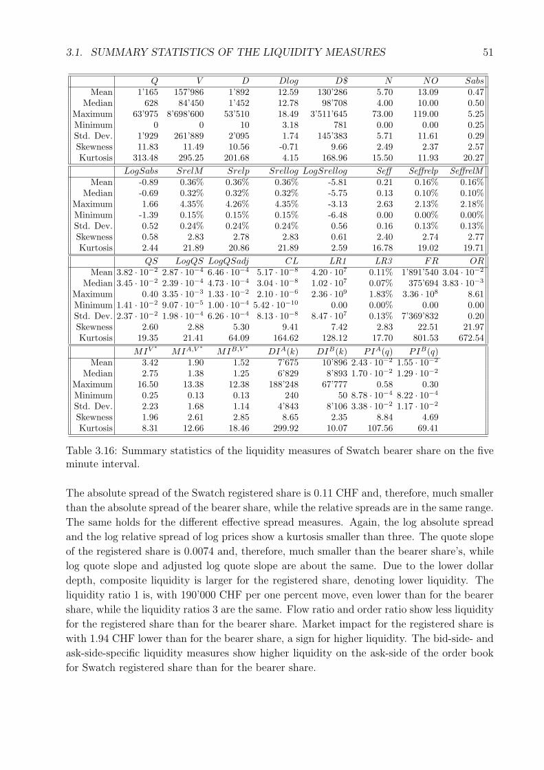
3.1. SUMMARY STATISTICS OF THE LIQUIDITY MEASURES 51
Q V D Dlog D$ N NO SabsMean 1’165 157’986 1’892 12.59 130’286 5.70 13.09 0.47
Median 628 84’450 1’452 12.78 98’708 4.00 10.00 0.50Maximum 63’975 8’698’600 53’510 18.49 3’511’645 73.00 119.00 5.25Minimum 0 0 10 3.18 781 0.00 0.00 0.25Std. Dev. 1’929 261’889 2’095 1.74 145’383 5.71 11.61 0.29Skewness 11.83 11.49 10.56 -0.71 9.66 2.49 2.37 2.57Kurtosis 313.48 295.25 201.68 4.15 168.96 15.50 11.93 20.27
LogSabs SrelM Srelp Srellog LogSrellog Seff Seffrelp SeffrelMMean -0.89 0.36% 0.36% 0.36% -5.81 0.21 0.16% 0.16%
Median -0.69 0.32% 0.32% 0.32% -5.75 0.13 0.10% 0.10%Maximum 1.66 4.35% 4.26% 4.35% -3.13 2.63 2.13% 2.18%Minimum -1.39 0.15% 0.15% 0.15% -6.48 0.00 0.00% 0.00%Std. Dev. 0.52 0.24% 0.24% 0.24% 0.56 0.16 0.13% 0.13%Skewness 0.58 2.83 2.78 2.83 0.61 2.40 2.74 2.77Kurtosis 2.44 21.89 20.86 21.89 2.59 16.78 19.02 19.71
QS LogQS LogQSadj CL LR1 LR3 FR ORMean 3.82 · 10−2 2.87 · 10−4 6.46 · 10−4 5.17 · 10−8 4.20 · 107 0.11% 1’891’540 3.04 · 10−2
Median 3.45 · 10−2 2.39 · 10−4 4.73 · 10−4 3.04 · 10−8 1.02 · 107 0.07% 375’694 3.83 · 10−3
Maximum 0.40 3.35 · 10−3 1.33 · 10−2 2.10 · 10−6 2.36 · 109 1.83% 3.36 · 108 8.61Minimum 1.41 · 10−2 9.07 · 10−5 1.00 · 10−4 5.42 · 10−10 0.00 0.00% 0.00 0.00Std. Dev. 2.37 · 10−2 1.98 · 10−4 6.26 · 10−4 8.13 · 10−8 8.47 · 107 0.13% 7’369’832 0.20Skewness 2.60 2.88 5.30 9.41 7.42 2.83 22.51 21.97Kurtosis 19.35 21.41 64.09 164.62 128.12 17.70 801.53 672.54
MIV ∗ MIA,V ∗ MIB,V ∗ DIA(k) DIB(k) PIA(q) PIB(q)Mean 3.42 1.90 1.52 7’675 10’896 2.43 · 10−2 1.55 · 10−2
Median 2.75 1.38 1.25 6’829 8’893 1.70 · 10−2 1.29 · 10−2
Maximum 16.50 13.38 12.38 188’248 67’777 0.58 0.30Minimum 0.25 0.13 0.13 240 50 8.78 · 10−4 8.22 · 10−4
Std. Dev. 2.23 1.68 1.14 4’843 8’106 3.38 · 10−2 1.17 · 10−2
Skewness 1.96 2.61 2.85 8.65 2.35 8.84 4.69Kurtosis 8.31 12.66 18.46 299.92 10.07 107.56 69.41
Table 3.16: Summary statistics of the liquidity measures of Swatch bearer share on the fiveminute interval.
The absolute spread of the Swatch registered share is 0.11 CHF and, therefore, much smaller
than the absolute spread of the bearer share, while the relative spreads are in the same range.
The same holds for the different effective spread measures. Again, the log absolute spread
and the log relative spread of log prices show a kurtosis smaller than three. The quote slope
of the registered share is 0.0074 and, therefore, much smaller than the bearer share’s, while
log quote slope and adjusted log quote slope are about the same. Due to the lower dollar
depth, composite liquidity is larger for the registered share, denoting lower liquidity. The
liquidity ratio 1 is, with 190’000 CHF per one percent move, even lower than for the bearer
share, while the liquidity ratios 3 are the same. Flow ratio and order ratio show less liquidity
for the registered share than for the bearer share. Market impact for the registered share is
with 1.94 CHF lower than for the bearer share, a sign for higher liquidity. The bid-side- and
ask-side-specific liquidity measures show higher liquidity on the ask-side of the order book
for Swatch registered share than for the bearer share.
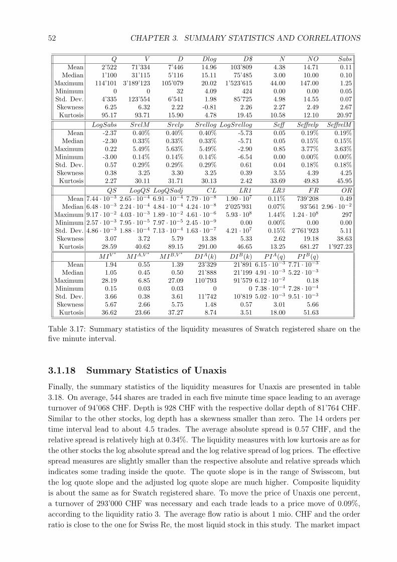
52 CHAPTER 3. SUMMARY STATISTICS AND CORRELATIONS
Q V D Dlog D$ N NO SabsMean 2’522 71’334 7’446 14.96 103’809 4.38 14.71 0.11
Median 1’100 31’115 5’116 15.11 75’485 3.00 10.00 0.10Maximum 114’101 3’189’123 105’079 20.02 1’523’615 44.00 147.00 1.25Minimum 0 0 32 4.09 424 0.00 0.00 0.05Std. Dev. 4’335 123’554 6’541 1.98 85’725 4.98 14.55 0.07Skewness 6.25 6.32 2.22 -0.81 2.26 2.27 2.49 2.67Kurtosis 95.17 93.71 15.90 4.78 19.45 10.58 12.10 20.97
LogSabs SrelM Srelp Srellog LogSrellog Seff Seffrelp SeffrelMMean -2.37 0.40% 0.40% 0.40% -5.73 0.05 0.19% 0.19%
Median -2.30 0.33% 0.33% 0.33% -5.71 0.05 0.15% 0.15%Maximum 0.22 5.49% 5.63% 5.49% -2.90 0.85 3.77% 3.63%Minimum -3.00 0.14% 0.14% 0.14% -6.54 0.00 0.00% 0.00%Std. Dev. 0.57 0.29% 0.29% 0.29% 0.61 0.04 0.18% 0.18%Skewness 0.38 3.25 3.30 3.25 0.39 3.55 4.39 4.25Kurtosis 2.27 30.11 31.71 30.13 2.42 33.69 49.83 45.95
QS LogQS LogQSadj CL LR1 LR3 FR ORMean 7.44 · 10−3 2.65 · 10−4 6.91 · 10−4 7.79 · 10−8 1.90 · 107 0.11% 739’208 0.49
Median 6.48 · 10−3 2.24 · 10−4 4.84 · 10−4 4.24 · 10−8 2’025’931 0.07% 93’561 2.96 · 10−2
Maximum 9.17 · 10−2 4.03 · 10−3 1.89 · 10−2 4.61 · 10−6 5.93 · 108 1.44% 1.24 · 108 297Minimum 2.57 · 10−3 7.95 · 10−5 7.97 · 10−5 2.45 · 10−9 0.00 0.00% 0.00 0.00Std. Dev. 4.86 · 10−3 1.88 · 10−4 7.13 · 10−4 1.63 · 10−7 4.21 · 107 0.15% 2’761’923 5.11Skewness 3.07 3.72 5.79 13.38 5.33 2.62 19.18 38.63Kurtosis 28.59 40.62 89.15 291.00 46.65 13.25 681.27 1’927.23
MIV ∗ MIA,V ∗ MIB,V ∗ DIA(k) DIB(k) PIA(q) PIB(q)Mean 1.94 0.55 1.39 23’329 21’891 6.15 · 10−3 7.71 · 10−3
Median 1.05 0.45 0.50 21’888 21’199 4.91 · 10−3 5.22 · 10−3
Maximum 28.19 6.85 27.09 110’793 91’579 6.12 · 10−2 0.18Minimum 0.15 0.03 0.03 0 0 7.38 · 10−4 7.28 · 10−4
Std. Dev. 3.66 0.38 3.61 11’742 10’819 5.02 · 10−3 9.51 · 10−3
Skewness 5.67 2.66 5.75 1.48 0.57 3.01 5.66Kurtosis 36.62 23.66 37.27 8.74 3.51 18.00 51.63
Table 3.17: Summary statistics of the liquidity measures of Swatch registered share on thefive minute interval.
3.1.18 Summary Statistics of Unaxis
Finally, the summary statistics of the liquidity measures for Unaxis are presented in table
3.18. On average, 544 shares are traded in each five minute time space leading to an average
turnover of 94’068 CHF. Depth is 928 CHF with the respective dollar depth of 81’764 CHF.
Similar to the other stocks, log depth has a skewness smaller than zero. The 14 orders per
time interval lead to about 4.5 trades. The average absolute spread is 0.57 CHF, and the
relative spread is relatively high at 0.34%. The liquidity measures with low kurtosis are as for
the other stocks the log absolute spread and the log relative spread of log prices. The effective
spread measures are slightly smaller than the respective absolute and relative spreads which
indicates some trading inside the quote. The quote slope is in the range of Swisscom, but
the log quote slope and the adjusted log quote slope are much higher. Composite liquidity
is about the same as for Swatch registered share. To move the price of Unaxis one percent,
a turnover of 293’000 CHF was necessary and each trade leads to a price move of 0.09%,
according to the liquidity ratio 3. The average flow ratio is about 1 mio. CHF and the order
ratio is close to the one for Swiss Re, the most liquid stock in this study. The market impact
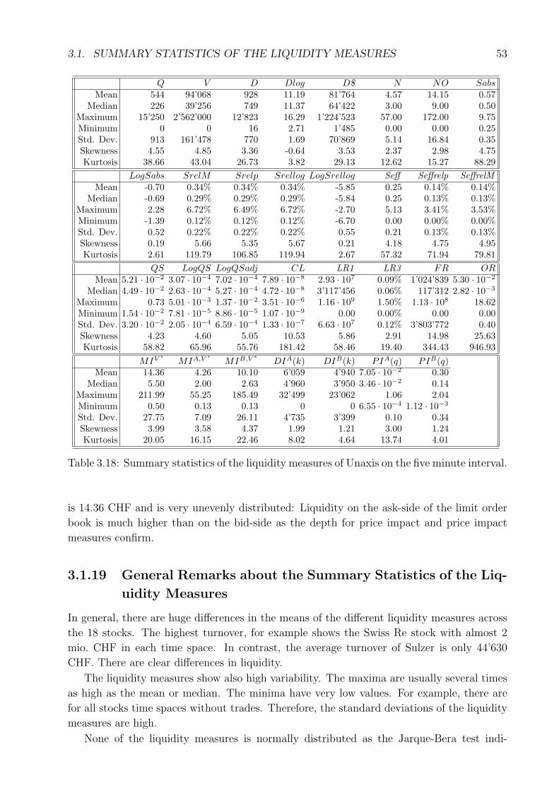
3.1. SUMMARY STATISTICS OF THE LIQUIDITY MEASURES 53
Q V D Dlog D$ N NO SabsMean 544 94’068 928 11.19 81’764 4.57 14.15 0.57
Median 226 39’256 749 11.37 64’422 3.00 9.00 0.50Maximum 15’250 2’562’000 12’823 16.29 1’224’523 57.00 172.00 9.75Minimum 0 0 16 2.71 1’485 0.00 0.00 0.25Std. Dev. 913 161’478 770 1.69 70’869 5.14 16.84 0.35Skewness 4.55 4.85 3.36 -0.64 3.53 2.37 2.98 4.75Kurtosis 38.66 43.04 26.73 3.82 29.13 12.62 15.27 88.29
LogSabs SrelM Srelp Srellog LogSrellog Seff Seffrelp SeffrelMMean -0.70 0.34% 0.34% 0.34% -5.85 0.25 0.14% 0.14%
Median -0.69 0.29% 0.29% 0.29% -5.84 0.25 0.13% 0.13%Maximum 2.28 6.72% 6.49% 6.72% -2.70 5.13 3.41% 3.53%Minimum -1.39 0.12% 0.12% 0.12% -6.70 0.00 0.00% 0.00%Std. Dev. 0.52 0.22% 0.22% 0.22% 0.55 0.21 0.13% 0.13%Skewness 0.19 5.66 5.35 5.67 0.21 4.18 4.75 4.95Kurtosis 2.61 119.79 106.85 119.94 2.67 57.32 71.94 79.81
QS LogQS LogQSadj CL LR1 LR3 FR ORMean 5.21 · 10−2 3.07 · 10−4 7.02 · 10−4 7.89 · 10−8 2.93 · 107 0.09% 1’024’839 5.30 · 10−2
Median 4.49 · 10−2 2.63 · 10−4 5.27 · 10−4 4.72 · 10−8 3’117’456 0.06% 117’312 2.82 · 10−3
Maximum 0.73 5.01 · 10−3 1.37 · 10−2 3.51 · 10−6 1.16 · 109 1.50% 1.13 · 108 18.62Minimum 1.54 · 10−2 7.81 · 10−5 8.86 · 10−5 1.07 · 10−9 0.00 0.00% 0.00 0.00Std. Dev. 3.20 · 10−2 2.05 · 10−4 6.59 · 10−4 1.33 · 10−7 6.63 · 107 0.12% 3’803’772 0.40Skewness 4.23 4.60 5.05 10.53 5.86 2.91 14.98 25.63Kurtosis 58.82 65.96 55.76 181.42 58.46 19.40 344.43 946.93
MIV ∗ MIA,V ∗ MIB,V ∗ DIA(k) DIB(k) PIA(q) PIB(q)Mean 14.36 4.26 10.10 6’059 4’940 7.05 · 10−2 0.30
Median 5.50 2.00 2.63 4’960 3’950 3.46 · 10−2 0.14Maximum 211.99 55.25 185.49 32’499 23’062 1.06 2.04Minimum 0.50 0.13 0.13 0 0 6.55 · 10−4 1.12 · 10−3
Std. Dev. 27.75 7.09 26.11 4’735 3’399 0.10 0.34Skewness 3.99 3.58 4.37 1.99 1.21 3.00 1.24Kurtosis 20.05 16.15 22.46 8.02 4.64 13.74 4.01
Table 3.18: Summary statistics of the liquidity measures of Unaxis on the five minute interval.
is 14.36 CHF and is very unevenly distributed: Liquidity on the ask-side of the limit order
book is much higher than on the bid-side as the depth for price impact and price impact
measures confirm.
3.1.19 General Remarks about the Summary Statistics of the Liq-
uidity Measures
In general, there are huge differences in the means of the different liquidity measures across
the 18 stocks. The highest turnover, for example shows the Swiss Re stock with almost 2
mio. CHF in each time space. In contrast, the average turnover of Sulzer is only 44’630
CHF. There are clear differences in liquidity.
The liquidity measures show also high variability. The maxima are usually several times
as high as the mean or median. The minima have very low values. For example, there are
for all stocks time spaces without trades. Therefore, the standard deviations of the liquidity
measures are high.
None of the liquidity measures is normally distributed as the Jarque-Bera test indi-
54 CHAPTER 3. SUMMARY STATISTICS AND CORRELATIONS
cates. In general, the mean is higher than median and the liquidity measures are, therefore,
right-skewed. With respect to the normal distribution they show fat-tails. To improve the
distributional properties of the liquidity measures I calculated the first differences from the
time series and calculated the principal component analysis and the vector autoregressive
model in the following chapters with these changes in liquidity.
3.2 Stock Ranking according to the Different Liquidity
Measures
Out of the liquidity measures, rankings are produced for the different stocks for each of the
31 liquidity measures. Table 3.19 shows these rankings. An entry of “1” in the table denotes,
that this stock is the most liquid according to the specific liquidity measure. If it has an
“18” it is the least liquid.
According to the rankings, Swiss Re is, on average, the most liquid stock as the last line
of table 3.19 shows. Its average rank is 2.81. Swiss Re is followed by Adecco with an average
rank of 4.00 and Richemont with 4.90. Swisscom, Ciba, Syngenta, Holcim, Clariant, Lonza,
Baer, Givaudan, Kudelski, Swatch registered share, Serono and Swatch bearer share are set
in the middle with average ranks between 6.35 and 12.65. Finally, Unaxis, Surveillance and
Sulzer are the least liquid stocks, on average.
The different rankings of the 31 liquidity measures are investigated for their correlation
using the Spearman rank correlation, rk:
rk = 1− 6 ·Rn · (n2 − 1)
(3.2)
R denotes the sum of the squared differences in ranks: R =n∑
i=1
di2i . n is the number
of observations which is eighteen in our case. To determine whether the correlations are
different from zero, they are compared to a special table of critical values for the Spearman
rank correlation test which can be found e.g. in Kanji (1999), p. 199. The methodology is
similar to Wang (2002) for different market impacts along the book.
Table 3.20 shows the rank correlations produced by the 31 liquidity measures for the
18 stocks. There seem to be two different groups of liquidity measures that produce high
correlations among the rankings of the different stocks:
Group one consists of: volume, depth and log depth, the number of orders and the
number of trades, the absolute and the log absolute spread, the effective spread, the quote
slope, the log quote slope and the adjusted log quote slope, the market impact, the depth
for price impact and the price impact measures. In general, these are the liquidity measures
that depend on the absolute stock price.
The second group which leads to similar rankings of the stocks consists of: turnover,
dollar depth, all the relative spread measures, composite liquidity, the liquidity ratio 1, the
liquidity ratio 3 and the flow ratio. This group of liquidity measures contains all the relative
spread measures. In general, these measures are independent of the stock price.
The ranking based on the order ratio is negatively correlated to about half of the other
rankings. With depth, log depth and the depth for price impact on the ask-side, those
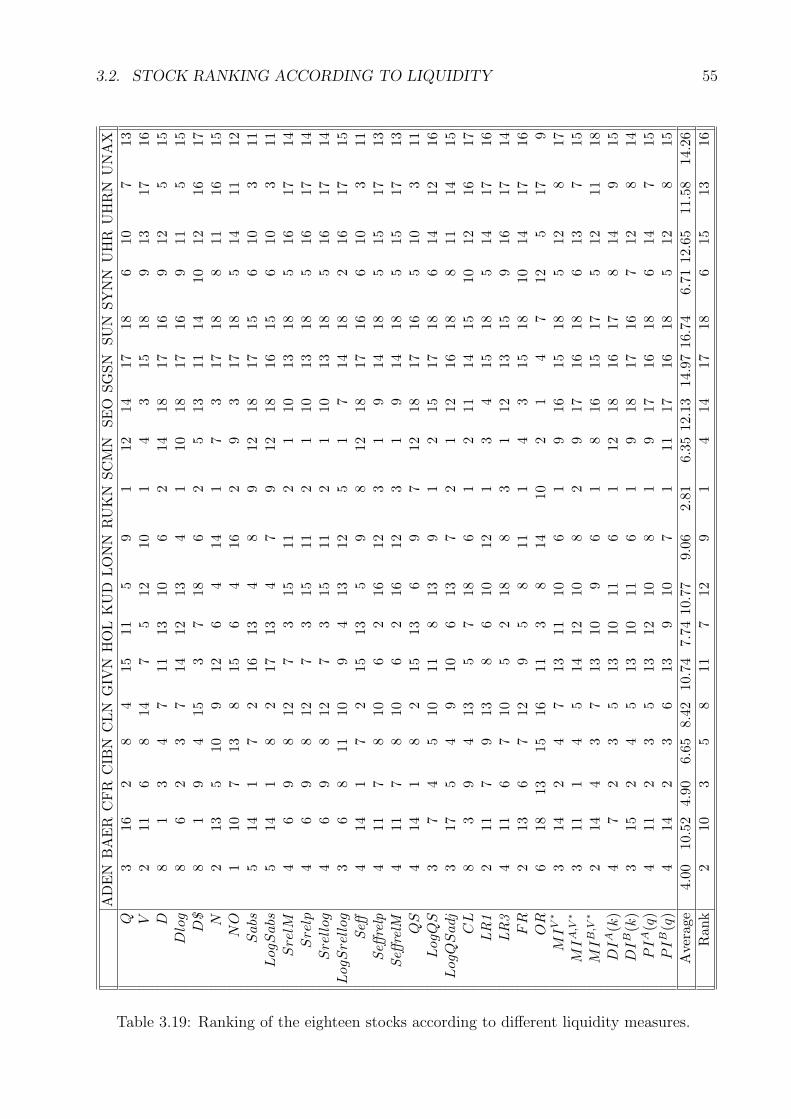
3.2. STOCK RANKING ACCORDING TO LIQUIDITY 55
AD
EN
BA
ER
CFR
CIB
NC
LN
GIV
NH
OL
KU
DLO
NN
RU
KN
SCM
NSE
OSG
SNSU
NSY
NN
UH
RU
HR
NU
NA
XQ
316
28
415
115
91
1214
1718
610
713
V2
116
814
75
1210
14
315
189
1317
16D
81
34
711
1310
62
1418
1716
912
515
Dlo
g8
62
37
1412
134
110
1817
169
115
15D
$8
19
415
37
186
25
1311
1410
1216
17N
213
510
912
64
141
73
1718
811
1615
NO
110
713
815
64
162
93
1718
514
1112
Sabs
514
17
216
134
89
1218
1715
610
311
Log
Sabs
514
18
217
134
79
1218
1615
610
311
Sre
lM4
69
812
73
1511
21
1013
185
1617
14S
relp
46
98
127
315
112
110
1318
516
1714
Sre
llog
46
98
127
315
112
110
1318
516
1714
Log
Sre
llog
36
811
109
413
125
17
1418
216
1715
Seff
414
17
215
135
98
1218
1716
610
311
Seffre
lp4
117
810
62
1612
31
914
185
1517
13Se
ffre
lM4
117
810
62
1612
31
914
185
1517
13Q
S4
141
82
1513
69
712
1817
165
103
11L
ogQ
S3
74
510
118
139
12
1517
186
1412
16L
ogQ
Sadj
317
54
910
613
72
112
1618
811
1415
CL
83
94
135
718
61
211
1415
1012
1617
LR
12
117
913
86
1012
13
415
185
1417
16LR
34
116
710
52
188
31
1213
159
1617
14F
R2
136
712
95
811
14
315
1810
1417
16O
R6
1813
1516
113
814
102
14
712
517
9M
IV∗
314
24
713
1110
61
916
1518
512
817
MI
A,V∗
311
14
514
1210
82
917
1618
613
715
MI
B,V∗
214
43
713
109
61
816
1517
512
1118
DI
A(k
)4
72
35
1310
116
112
1816
178
149
15D
IB
(k)
315
24
513
1011
61
918
1716
712
814
PI
A(q
)4
112
35
1312
108
19
1716
186
147
15P
IB
(q)
414
23
613
910
71
1117
1618
512
815
Ave
rage
4.00
10.5
24.
906.
658.
4210
.74
7.74
10.7
79.
062.
816.
3512
.13
14.9
716
.74
6.71
12.6
511
.58
14.2
6R
ank
210
35
811
712
91
414
1718
615
1316
Table 3.19: Ranking of the eighteen stocks according to different liquidity measures.
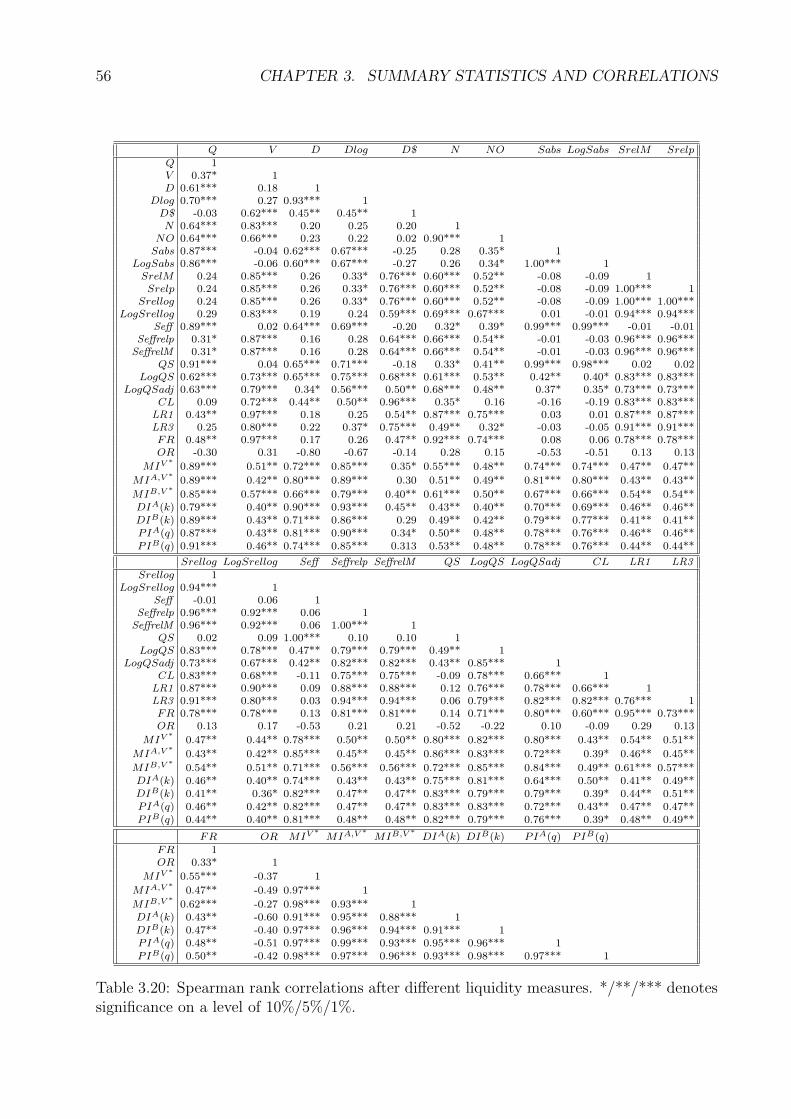
56 CHAPTER 3. SUMMARY STATISTICS AND CORRELATIONS
Q V D Dlog D$ N NO Sabs LogSabs SrelM SrelpQ 1V 0.37* 1D 0.61*** 0.18 1
Dlog 0.70*** 0.27 0.93*** 1D$ -0.03 0.62*** 0.45** 0.45** 1N 0.64*** 0.83*** 0.20 0.25 0.20 1
NO 0.64*** 0.66*** 0.23 0.22 0.02 0.90*** 1Sabs 0.87*** -0.04 0.62*** 0.67*** -0.25 0.28 0.35* 1
LogSabs 0.86*** -0.06 0.60*** 0.67*** -0.27 0.26 0.34* 1.00*** 1SrelM 0.24 0.85*** 0.26 0.33* 0.76*** 0.60*** 0.52** -0.08 -0.09 1Srelp 0.24 0.85*** 0.26 0.33* 0.76*** 0.60*** 0.52** -0.08 -0.09 1.00*** 1
Srellog 0.24 0.85*** 0.26 0.33* 0.76*** 0.60*** 0.52** -0.08 -0.09 1.00*** 1.00***LogSrellog 0.29 0.83*** 0.19 0.24 0.59*** 0.69*** 0.67*** 0.01 -0.01 0.94*** 0.94***
Seff 0.89*** 0.02 0.64*** 0.69*** -0.20 0.32* 0.39* 0.99*** 0.99*** -0.01 -0.01Seffrelp 0.31* 0.87*** 0.16 0.28 0.64*** 0.66*** 0.54** -0.01 -0.03 0.96*** 0.96***
SeffrelM 0.31* 0.87*** 0.16 0.28 0.64*** 0.66*** 0.54** -0.01 -0.03 0.96*** 0.96***QS 0.91*** 0.04 0.65*** 0.71*** -0.18 0.33* 0.41** 0.99*** 0.98*** 0.02 0.02
LogQS 0.62*** 0.73*** 0.65*** 0.75*** 0.68*** 0.61*** 0.53** 0.42** 0.40* 0.83*** 0.83***LogQSadj 0.63*** 0.79*** 0.34* 0.56*** 0.50** 0.68*** 0.48** 0.37* 0.35* 0.73*** 0.73***
CL 0.09 0.72*** 0.44** 0.50** 0.96*** 0.35* 0.16 -0.16 -0.19 0.83*** 0.83***LR1 0.43** 0.97*** 0.18 0.25 0.54** 0.87*** 0.75*** 0.03 0.01 0.87*** 0.87***LR3 0.25 0.80*** 0.22 0.37* 0.75*** 0.49** 0.32* -0.03 -0.05 0.91*** 0.91***FR 0.48** 0.97*** 0.17 0.26 0.47** 0.92*** 0.74*** 0.08 0.06 0.78*** 0.78***OR -0.30 0.31 -0.80 -0.67 -0.14 0.28 0.15 -0.53 -0.51 0.13 0.13
MIV ∗ 0.89*** 0.51** 0.72*** 0.85*** 0.35* 0.55*** 0.48** 0.74*** 0.74*** 0.47** 0.47**
MIA,V ∗ 0.89*** 0.42** 0.80*** 0.89*** 0.30 0.51** 0.49** 0.81*** 0.80*** 0.43** 0.43**
MIB,V ∗ 0.85*** 0.57*** 0.66*** 0.79*** 0.40** 0.61*** 0.50** 0.67*** 0.66*** 0.54** 0.54**DIA(k) 0.79*** 0.40** 0.90*** 0.93*** 0.45** 0.43** 0.40** 0.70*** 0.69*** 0.46** 0.46**DIB(k) 0.89*** 0.43** 0.71*** 0.86*** 0.29 0.49** 0.42** 0.79*** 0.77*** 0.41** 0.41**PIA(q) 0.87*** 0.43** 0.81*** 0.90*** 0.34* 0.50** 0.48** 0.78*** 0.76*** 0.46** 0.46**PIB(q) 0.91*** 0.46** 0.74*** 0.85*** 0.313 0.53** 0.48** 0.78*** 0.76*** 0.44** 0.44**
Srellog LogSrellog Seff Seffrelp SeffrelM QS LogQS LogQSadj CL LR1 LR3Srellog 1
LogSrellog 0.94*** 1Seff -0.01 0.06 1
Seffrelp 0.96*** 0.92*** 0.06 1SeffrelM 0.96*** 0.92*** 0.06 1.00*** 1
QS 0.02 0.09 1.00*** 0.10 0.10 1LogQS 0.83*** 0.78*** 0.47** 0.79*** 0.79*** 0.49** 1
LogQSadj 0.73*** 0.67*** 0.42** 0.82*** 0.82*** 0.43** 0.85*** 1CL 0.83*** 0.68*** -0.11 0.75*** 0.75*** -0.09 0.78*** 0.66*** 1
LR1 0.87*** 0.90*** 0.09 0.88*** 0.88*** 0.12 0.76*** 0.78*** 0.66*** 1LR3 0.91*** 0.80*** 0.03 0.94*** 0.94*** 0.06 0.79*** 0.82*** 0.82*** 0.76*** 1FR 0.78*** 0.78*** 0.13 0.81*** 0.81*** 0.14 0.71*** 0.80*** 0.60*** 0.95*** 0.73***OR 0.13 0.17 -0.53 0.21 0.21 -0.52 -0.22 0.10 -0.09 0.29 0.13
MIV ∗ 0.47** 0.44** 0.78*** 0.50** 0.50** 0.80*** 0.82*** 0.80*** 0.43** 0.54** 0.51**
MIA,V ∗ 0.43** 0.42** 0.85*** 0.45** 0.45** 0.86*** 0.83*** 0.72*** 0.39* 0.46** 0.45**
MIB,V ∗ 0.54** 0.51** 0.71*** 0.56*** 0.56*** 0.72*** 0.85*** 0.84*** 0.49** 0.61*** 0.57***DIA(k) 0.46** 0.40** 0.74*** 0.43** 0.43** 0.75*** 0.81*** 0.64*** 0.50** 0.41** 0.49**DIB(k) 0.41** 0.36* 0.82*** 0.47** 0.47** 0.83*** 0.79*** 0.79*** 0.39* 0.44** 0.51**PIA(q) 0.46** 0.42** 0.82*** 0.47** 0.47** 0.83*** 0.83*** 0.72*** 0.43** 0.47** 0.47**PIB(q) 0.44** 0.40** 0.81*** 0.48** 0.48** 0.82*** 0.79*** 0.76*** 0.39* 0.48** 0.49**
FR OR MIV ∗ MIA,V ∗ MIB,V ∗ DIA(k) DIB(k) PIA(q) PIB(q)FR 1OR 0.33* 1
MIV ∗ 0.55*** -0.37 1
MIA,V ∗ 0.47** -0.49 0.97*** 1
MIB,V ∗ 0.62*** -0.27 0.98*** 0.93*** 1DIA(k) 0.43** -0.60 0.91*** 0.95*** 0.88*** 1DIB(k) 0.47** -0.40 0.97*** 0.96*** 0.94*** 0.91*** 1PIA(q) 0.48** -0.51 0.97*** 0.99*** 0.93*** 0.95*** 0.96*** 1PIB(q) 0.50** -0.42 0.98*** 0.97*** 0.96*** 0.93*** 0.98*** 0.97*** 1
Table 3.20: Spearman rank correlations after different liquidity measures. */**/*** denotessignificance on a level of 10%/5%/1%.
3.3. CORRELATIONS OF THE LIQUIDITY MEASURES 57
negative correlations are even significant, at least, at a 5% level.
3.3 Correlations of the Liquidity Measures
For each stock, the correlations of the liquidity measures were calculated. They can be found
in appendix C. The average correlations of the liquidity measures for the eighteen stocks are
presented in table 3.21. Liquidity measures that are highly correlated to others and from
the analysis are listed below.
• Volume: It is highly correlated with turnover. Turnover is comparable across stocks
with different share prices, while volume is not.
• Depth: It has an average correlation of 0.99 to dollar depth and, once again, dollar
depth is comparable across different stocks: Therefore, depth is dropped.
• Absolute spread: It is correlated with a variety of liquidity measures. Its correlation
to the relative spreads is 0.98, and, therefore, the absolute spread is dropped from the
sample.
• Relative spread with last trade: The correlation of the relative spread with the mid
price and the last trade is unity. Because the relative spread with the mid price always
can be calculated it is retained.
• Relative spread of log prices: It has a correlation of 0.93 to the log relative spread of
log prices and to the quote slope. The average correlation to the log quote slope is
even higher. The relative spread of log prices is, therefore, dropped from the liquidity
measures.
• Effective spread: It is highly correlated with the relative effective spreads and elimi-
nated.
• Relative effective spread with last trade: The relative effective spread with last trade
and the mid price have a correlation of unity. The relative effective spread with last
trade is dropped.
• Quote slope and log quote slope are correlated with 0.98 and the log quote slope is
dropped.
The results are in line with Irvine et al. (2000) which report negative correlations between
the market impact measures and depth, too. Also the correlation between the market impact
measures and the relative effective spread is confirmed. On the other hand, the correlation
between the relative spread and the market impact measures is higher in their paper.
After this section, I conclude that only the following 23 liquidity measures are needed:
turnover, log depth, dollar depth, number of trades and number of orders, the log absolute
spread, the relative spread with the mid price, the log relative spread of log prices, the relative
spread with the mid price, quote slope, adjusted log quote slope, composite liquidity, the
liquidity ratios 1 and 3, the flow ratio, order ratio, the market impact measures, the depth
for price impact measures and finally, the price impact measures. With these measures I
continue.
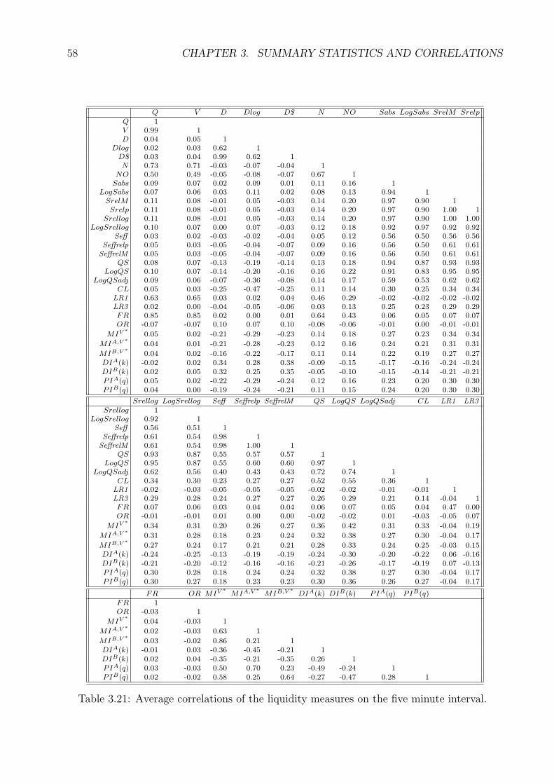
58 CHAPTER 3. SUMMARY STATISTICS AND CORRELATIONS
Q V D Dlog D$ N NO Sabs LogSabs SrelM SrelpQ 1V 0.99 1D 0.04 0.05 1
Dlog 0.02 0.03 0.62 1D$ 0.03 0.04 0.99 0.62 1N 0.73 0.71 -0.03 -0.07 -0.04 1
NO 0.50 0.49 -0.05 -0.08 -0.07 0.67 1Sabs 0.09 0.07 0.02 0.09 0.01 0.11 0.16 1
LogSabs 0.07 0.06 0.03 0.11 0.02 0.08 0.13 0.94 1SrelM 0.11 0.08 -0.01 0.05 -0.03 0.14 0.20 0.97 0.90 1Srelp 0.11 0.08 -0.01 0.05 -0.03 0.14 0.20 0.97 0.90 1.00 1
Srellog 0.11 0.08 -0.01 0.05 -0.03 0.14 0.20 0.97 0.90 1.00 1.00LogSrellog 0.10 0.07 0.00 0.07 -0.03 0.12 0.18 0.92 0.97 0.92 0.92
Seff 0.03 0.02 -0.03 -0.02 -0.04 0.05 0.12 0.56 0.50 0.56 0.56Seffrelp 0.05 0.03 -0.05 -0.04 -0.07 0.09 0.16 0.56 0.50 0.61 0.61
SeffrelM 0.05 0.03 -0.05 -0.04 -0.07 0.09 0.16 0.56 0.50 0.61 0.61QS 0.08 0.07 -0.13 -0.19 -0.14 0.13 0.18 0.94 0.87 0.93 0.93
LogQS 0.10 0.07 -0.14 -0.20 -0.16 0.16 0.22 0.91 0.83 0.95 0.95LogQSadj 0.09 0.06 -0.07 -0.36 -0.08 0.14 0.17 0.59 0.53 0.62 0.62
CL 0.05 0.03 -0.25 -0.47 -0.25 0.11 0.14 0.30 0.25 0.34 0.34LR1 0.63 0.65 0.03 0.02 0.04 0.46 0.29 -0.02 -0.02 -0.02 -0.02LR3 0.02 0.00 -0.04 -0.05 -0.06 0.03 0.13 0.25 0.23 0.29 0.29FR 0.85 0.85 0.02 0.00 0.01 0.64 0.43 0.06 0.05 0.07 0.07OR -0.07 -0.07 0.10 0.07 0.10 -0.08 -0.06 -0.01 0.00 -0.01 -0.01
MIV ∗ 0.05 0.02 -0.21 -0.29 -0.23 0.14 0.18 0.27 0.23 0.34 0.34
MIA,V ∗ 0.04 0.01 -0.21 -0.28 -0.23 0.12 0.16 0.24 0.21 0.31 0.31
MIB,V ∗ 0.04 0.02 -0.16 -0.22 -0.17 0.11 0.14 0.22 0.19 0.27 0.27DIA(k) -0.02 0.02 0.34 0.28 0.38 -0.09 -0.15 -0.17 -0.16 -0.24 -0.24DIB(k) 0.02 0.05 0.32 0.25 0.35 -0.05 -0.10 -0.15 -0.14 -0.21 -0.21PIA(q) 0.05 0.02 -0.22 -0.29 -0.24 0.12 0.16 0.23 0.20 0.30 0.30PIB(q) 0.04 0.00 -0.19 -0.24 -0.21 0.11 0.15 0.24 0.20 0.30 0.30
Srellog LogSrellog Seff Seffrelp SeffrelM QS LogQS LogQSadj CL LR1 LR3Srellog 1
LogSrellog 0.92 1Seff 0.56 0.51 1
Seffrelp 0.61 0.54 0.98 1SeffrelM 0.61 0.54 0.98 1.00 1
QS 0.93 0.87 0.55 0.57 0.57 1LogQS 0.95 0.87 0.55 0.60 0.60 0.97 1
LogQSadj 0.62 0.56 0.40 0.43 0.43 0.72 0.74 1CL 0.34 0.30 0.23 0.27 0.27 0.52 0.55 0.36 1
LR1 -0.02 -0.03 -0.05 -0.05 -0.05 -0.02 -0.02 -0.01 -0.01 1LR3 0.29 0.28 0.24 0.27 0.27 0.26 0.29 0.21 0.14 -0.04 1FR 0.07 0.06 0.03 0.04 0.04 0.06 0.07 0.05 0.04 0.47 0.00OR -0.01 -0.01 0.01 0.00 0.00 -0.02 -0.02 0.01 -0.03 -0.05 0.07
MIV ∗ 0.34 0.31 0.20 0.26 0.27 0.36 0.42 0.31 0.33 -0.04 0.19
MIA,V ∗ 0.31 0.28 0.18 0.23 0.24 0.32 0.38 0.27 0.30 -0.04 0.17
MIB,V ∗ 0.27 0.24 0.17 0.21 0.21 0.28 0.33 0.24 0.25 -0.03 0.15DIA(k) -0.24 -0.25 -0.13 -0.19 -0.19 -0.24 -0.30 -0.20 -0.22 0.06 -0.16DIB(k) -0.21 -0.20 -0.12 -0.16 -0.16 -0.21 -0.26 -0.17 -0.19 0.07 -0.13PIA(q) 0.30 0.28 0.18 0.24 0.24 0.32 0.38 0.27 0.30 -0.04 0.17PIB(q) 0.30 0.27 0.18 0.23 0.23 0.30 0.36 0.26 0.27 -0.04 0.17
FR OR MIV ∗ MIA,V ∗ MIB,V ∗ DIA(k) DIB(k) PIA(q) PIB(q)FR 1OR -0.03 1
MIV ∗ 0.04 -0.03 1
MIA,V ∗ 0.02 -0.03 0.63 1
MIB,V ∗ 0.03 -0.02 0.86 0.21 1DIA(k) -0.01 0.03 -0.36 -0.45 -0.21 1DIB(k) 0.02 0.04 -0.35 -0.21 -0.35 0.26 1PIA(q) 0.03 -0.03 0.50 0.70 0.23 -0.49 -0.24 1PIB(q) 0.02 -0.02 0.58 0.25 0.64 -0.27 -0.47 0.28 1
Table 3.21: Average correlations of the liquidity measures on the five minute interval.
Chapter 4
Principal Component Analysis of
Liquidity Measures
To extract common factors from the 23 remaining liquidity measures, in this chapter a
principal component analysis is carried out. Section 4.1 describes briefly the methodology,
while the sections 4.2 to 4.19 present the results of the principal component analysis for each
of the 18 stocks. Section 4.20 draws some conclusions and determines the liquidity measures
necessary to capture all the dimensions of liquidity.
4.1 Principal Component Analysis
Principal component analysis dates back to Pearson (1901) and Hotelling (1933). It is
used to examine the relationships among several variables and to reduce the complexity.
The number of variables is reduced to a set of a few factors that are able to explain the
dynamics of the liquidity measures. It detects linear relationships. The complete factor
solution is calculated; this means that the n liquidity measures are explained by n principal
components. The principal components are the factors. The first principal component is
calculated as the linear combination of the liquidity measures:
F1 = b11 ·m1 + b12 ·m2 + ... + b1n ·mn (4.1)
F1 must have maximal variance. Because variance rises with rising b, it is limited by the
following constraint:
b211 + b2
12 + ... + b21n = 1 (4.2)
F is called factor scores. The solution for b1 equals the eigenvector with the largest
eigenvalue of the variance-covariance matrix. This means that the first principal component
accounts for the greatest possible variance. When the first principal component is found,
the calculation is repeated for the second principal component with the additional constraint
that it is orthogonal to the first principal component. The solution for b2 now equals the
eigenvector with the second largest eigenvalue, which has again the greatest possible vari-
ance. This procedure is repeated until the nth principal component is found. Basically, the
eigenvectors of the variance-covariance-matrix of the liquidity measures have to be found.
59
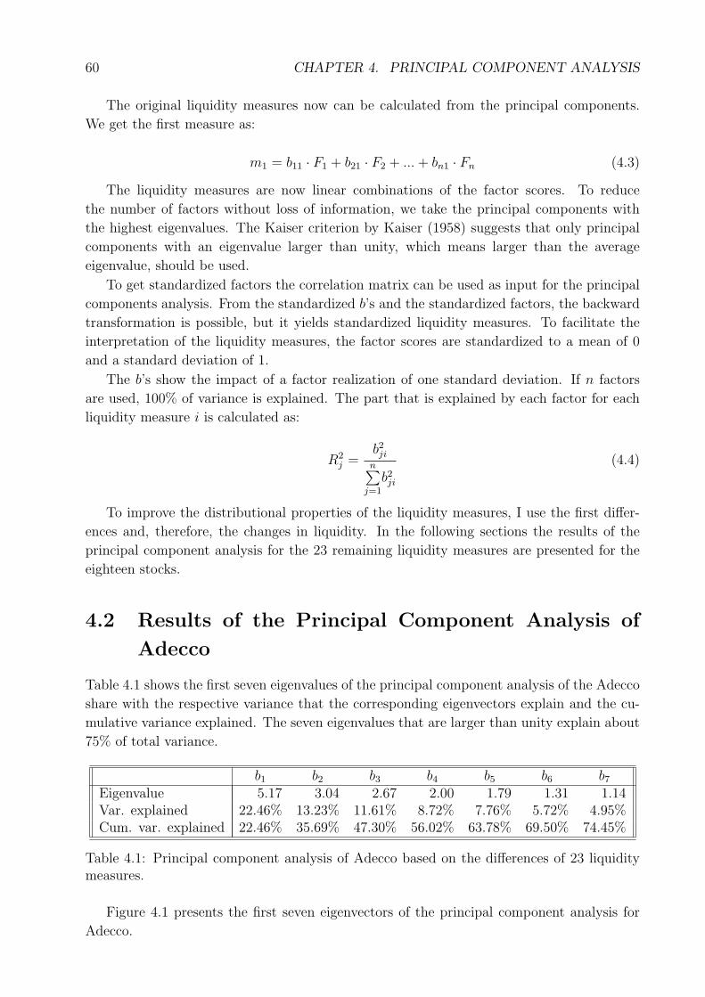
60 CHAPTER 4. PRINCIPAL COMPONENT ANALYSIS
The original liquidity measures now can be calculated from the principal components.
We get the first measure as:
m1 = b11 · F1 + b21 · F2 + ... + bn1 · Fn (4.3)
The liquidity measures are now linear combinations of the factor scores. To reduce
the number of factors without loss of information, we take the principal components with
the highest eigenvalues. The Kaiser criterion by Kaiser (1958) suggests that only principal
components with an eigenvalue larger than unity, which means larger than the average
eigenvalue, should be used.
To get standardized factors the correlation matrix can be used as input for the principal
components analysis. From the standardized b’s and the standardized factors, the backward
transformation is possible, but it yields standardized liquidity measures. To facilitate the
interpretation of the liquidity measures, the factor scores are standardized to a mean of 0
and a standard deviation of 1.
The b’s show the impact of a factor realization of one standard deviation. If n factors
are used, 100% of variance is explained. The part that is explained by each factor for each
liquidity measure i is calculated as:
R2j =
b2ji
n∑j=1
b2ji
(4.4)
To improve the distributional properties of the liquidity measures, I use the first differ-
ences and, therefore, the changes in liquidity. In the following sections the results of the
principal component analysis for the 23 remaining liquidity measures are presented for the
eighteen stocks.
4.2 Results of the Principal Component Analysis of
Adecco
Table 4.1 shows the first seven eigenvalues of the principal component analysis of the Adecco
share with the respective variance that the corresponding eigenvectors explain and the cu-
mulative variance explained. The seven eigenvalues that are larger than unity explain about
75% of total variance.
b1 b2 b3 b4 b5 b6 b7
Eigenvalue 5.17 3.04 2.67 2.00 1.79 1.31 1.14Var. explained 22.46% 13.23% 11.61% 8.72% 7.76% 5.72% 4.95%Cum. var. explained 22.46% 35.69% 47.30% 56.02% 63.78% 69.50% 74.45%
Table 4.1: Principal component analysis of Adecco based on the differences of 23 liquiditymeasures.
Figure 4.1 presents the first seven eigenvectors of the principal component analysis for
Adecco.
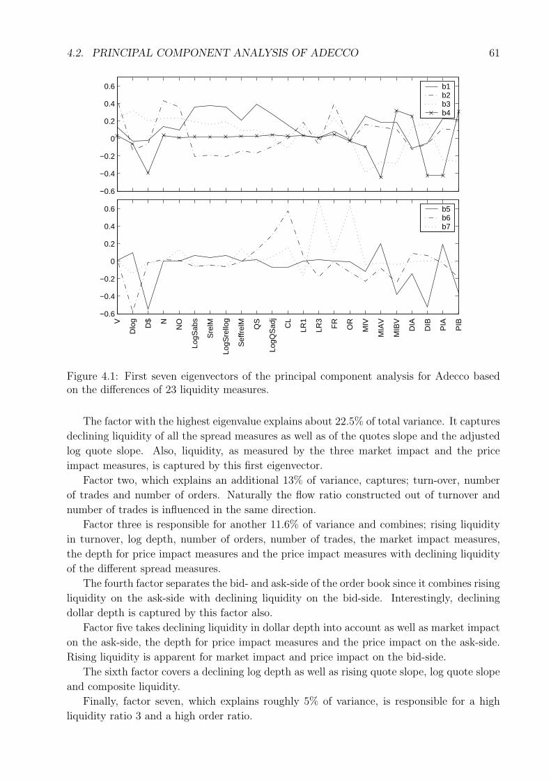
4.2. PRINCIPAL COMPONENT ANALYSIS OF ADECCO 61
−0.6
−0.4
−0.2
0
0.2
0.4
0.6 b1b2b3b4
−0.6
−0.4
−0.2
0
0.2
0.4
0.6
V
Dlo
g
D$ N
NO
LogS
abs
Sre
lM
LogS
rello
g
Sef
frel
M
QS
LogQ
Sad
j
CL
LR1
LR3
FR
OR
MIV
MIA
V
MIB
V
DIA
DIB
PIA
PIB
b5b6b7
Figure 4.1: First seven eigenvectors of the principal component analysis for Adecco basedon the differences of 23 liquidity measures.
The factor with the highest eigenvalue explains about 22.5% of total variance. It captures
declining liquidity of all the spread measures as well as of the quotes slope and the adjusted
log quote slope. Also, liquidity, as measured by the three market impact and the price
impact measures, is captured by this first eigenvector.
Factor two, which explains an additional 13% of variance, captures; turn-over, number
of trades and number of orders. Naturally the flow ratio constructed out of turnover and
number of trades is influenced in the same direction.
Factor three is responsible for another 11.6% of variance and combines; rising liquidity
in turnover, log depth, number of orders, number of trades, the market impact measures,
the depth for price impact measures and the price impact measures with declining liquidity
of the different spread measures.
The fourth factor separates the bid- and ask-side of the order book since it combines rising
liquidity on the ask-side with declining liquidity on the bid-side. Interestingly, declining
dollar depth is captured by this factor also.
Factor five takes declining liquidity in dollar depth into account as well as market impact
on the ask-side, the depth for price impact measures and the price impact on the ask-side.
Rising liquidity is apparent for market impact and price impact on the bid-side.
The sixth factor covers a declining log depth as well as rising quote slope, log quote slope
and composite liquidity.
Finally, factor seven, which explains roughly 5% of variance, is responsible for a high
liquidity ratio 3 and a high order ratio.
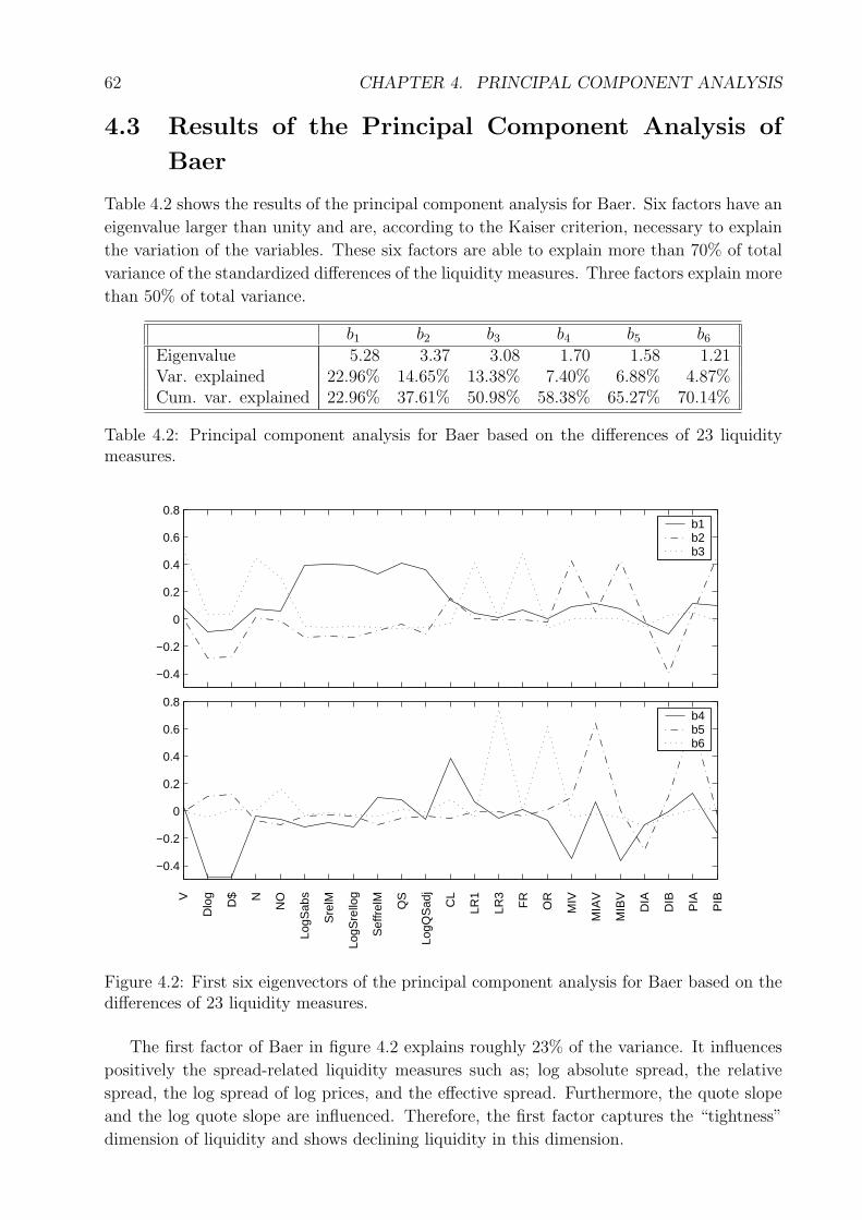
62 CHAPTER 4. PRINCIPAL COMPONENT ANALYSIS
4.3 Results of the Principal Component Analysis of
Baer
Table 4.2 shows the results of the principal component analysis for Baer. Six factors have an
eigenvalue larger than unity and are, according to the Kaiser criterion, necessary to explain
the variation of the variables. These six factors are able to explain more than 70% of total
variance of the standardized differences of the liquidity measures. Three factors explain more
than 50% of total variance.
b1 b2 b3 b4 b5 b6
Eigenvalue 5.28 3.37 3.08 1.70 1.58 1.21Var. explained 22.96% 14.65% 13.38% 7.40% 6.88% 4.87%Cum. var. explained 22.96% 37.61% 50.98% 58.38% 65.27% 70.14%
Table 4.2: Principal component analysis for Baer based on the differences of 23 liquiditymeasures.
−0.4
−0.2
0
0.2
0.4
0.6
0.8b1b2b3
−0.4
−0.2
0
0.2
0.4
0.6
0.8
V
Dlo
g
D$ N
NO
LogS
abs
Sre
lM
LogS
rello
g
Sef
frel
M
QS
LogQ
Sad
j
CL
LR1
LR3
FR
OR
MIV
MIA
V
MIB
V
DIA
DIB
PIA
PIB
b4b5b6
Figure 4.2: First six eigenvectors of the principal component analysis for Baer based on thedifferences of 23 liquidity measures.
The first factor of Baer in figure 4.2 explains roughly 23% of the variance. It influences
positively the spread-related liquidity measures such as; log absolute spread, the relative
spread, the log spread of log prices, and the effective spread. Furthermore, the quote slope
and the log quote slope are influenced. Therefore, the first factor captures the “tightness”
dimension of liquidity and shows declining liquidity in this dimension.
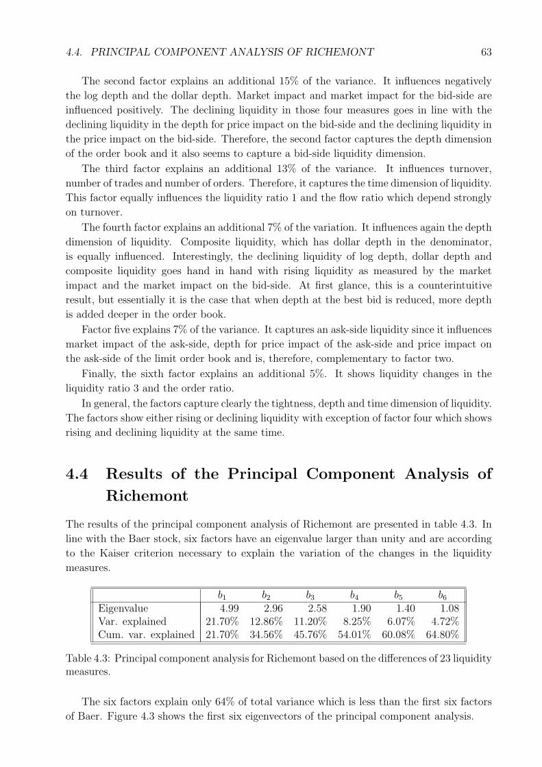
4.4. PRINCIPAL COMPONENT ANALYSIS OF RICHEMONT 63
The second factor explains an additional 15% of the variance. It influences negatively
the log depth and the dollar depth. Market impact and market impact for the bid-side are
influenced positively. The declining liquidity in those four measures goes in line with the
declining liquidity in the depth for price impact on the bid-side and the declining liquidity in
the price impact on the bid-side. Therefore, the second factor captures the depth dimension
of the order book and it also seems to capture a bid-side liquidity dimension.
The third factor explains an additional 13% of the variance. It influences turnover,
number of trades and number of orders. Therefore, it captures the time dimension of liquidity.
This factor equally influences the liquidity ratio 1 and the flow ratio which depend strongly
on turnover.
The fourth factor explains an additional 7% of the variation. It influences again the depth
dimension of liquidity. Composite liquidity, which has dollar depth in the denominator,
is equally influenced. Interestingly, the declining liquidity of log depth, dollar depth and
composite liquidity goes hand in hand with rising liquidity as measured by the market
impact and the market impact on the bid-side. At first glance, this is a counterintuitive
result, but essentially it is the case that when depth at the best bid is reduced, more depth
is added deeper in the order book.
Factor five explains 7% of the variance. It captures an ask-side liquidity since it influences
market impact of the ask-side, depth for price impact of the ask-side and price impact on
the ask-side of the limit order book and is, therefore, complementary to factor two.
Finally, the sixth factor explains an additional 5%. It shows liquidity changes in the
liquidity ratio 3 and the order ratio.
In general, the factors capture clearly the tightness, depth and time dimension of liquidity.
The factors show either rising or declining liquidity with exception of factor four which shows
rising and declining liquidity at the same time.
4.4 Results of the Principal Component Analysis of
Richemont
The results of the principal component analysis of Richemont are presented in table 4.3. In
line with the Baer stock, six factors have an eigenvalue larger than unity and are according
to the Kaiser criterion necessary to explain the variation of the changes in the liquidity
measures.
b1 b2 b3 b4 b5 b6
Eigenvalue 4.99 2.96 2.58 1.90 1.40 1.08Var. explained 21.70% 12.86% 11.20% 8.25% 6.07% 4.72%Cum. var. explained 21.70% 34.56% 45.76% 54.01% 60.08% 64.80%
Table 4.3: Principal component analysis for Richemont based on the differences of 23 liquiditymeasures.
The six factors explain only 64% of total variance which is less than the first six factors
of Baer. Figure 4.3 shows the first six eigenvectors of the principal component analysis.
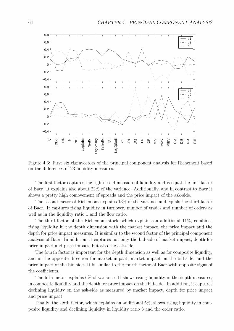
64 CHAPTER 4. PRINCIPAL COMPONENT ANALYSIS
−0.4
−0.2
0
0.2
0.4
0.6
0.8b1b2b3
−0.4
−0.2
0
0.2
0.4
0.6
0.8
V
Dlo
g
D$ N
NO
LogS
abs
Sre
lM
LogS
rello
g
Sef
frel
M
QS
LogQ
Sad
j
CL
LR1
LR3
FR
OR
MIV
MIA
V
MIB
V
DIA
DIB
PIA
PIB
b4b5b6
Figure 4.3: First six eigenvectors of the principal component analysis for Richemont basedon the differences of 23 liquidity measures.
The first factor captures the tightness dimension of liquidity and is equal the first factor
of Baer. It explains also about 22% of the variance. Additionally, and in contrast to Baer it
shows a pretty high comovement of spreads and the price impact of the ask-side.
The second factor of Richemont explains 13% of the variance and equals the third factor
of Baer. It captures rising liquidity in turnover, number of trades and number of orders as
well as in the liquidity ratio 1 and the flow ratio.
The third factor of the Richemont stock, which explains an additional 11%, combines
rising liquidity in the depth dimension with the market impact, the price impact and the
depth for price impact measures. It is similar to the second factor of the principal component
analysis of Baer. In addition, it captures not only the bid-side of market impact, depth for
price impact and price impact, but also the ask-side.
The fourth factor is important for the depth dimension as well as for composite liquidity,
and in the opposite direction for market impact, market impact on the bid-side, and the
price impact of the bid-side. It is similar to the fourth factor of Baer with opposite signs of
the coefficients.
The fifth factor explains 6% of variance. It shows rising liquidity in the depth measures,
in composite liquidity and the depth for price impact on the bid-side. In addition, it captures
declining liquidity on the ask-side as measured by market impact, depth for price impact
and price impact.
Finally, the sixth factor, which explains an additional 5%, shows rising liquidity in com-
posite liquidity and declining liquidity in liquidity ratio 3 and the order ratio.
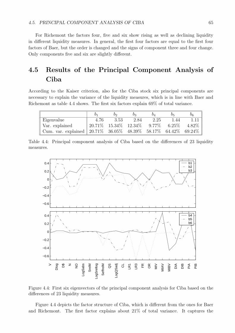
4.5. PRINCIPAL COMPONENT ANALYSIS OF CIBA 65
For Richemont the factors four, five and six show rising as well as declining liquidity
in different liquidity measures. In general, the first four factors are equal to the first four
factors of Baer, but the order is changed and the signs of component three and four change.
Only components five and six are slightly different.
4.5 Results of the Principal Component Analysis of
Ciba
According to the Kaiser criterion, also for the Ciba stock six principal components are
necessary to explain the variance of the liquidity measures, which is in line with Baer and
Richemont as table 4.4 shows. The first six factors explain 69% of total variance.
b1 b2 b3 b4 b5 b6
Eigenvalue 4.76 3.53 2.84 2.25 1.44 1.11Var. explained 20.71% 15.34% 12.34% 9.77% 6.25% 4.82%Cum. var. explained 20.71% 36.05% 48.39% 58.17% 64.42% 69.24%
Table 4.4: Principal component analysis of Ciba based on the differences of 23 liquiditymeasures.
−0.6
−0.4
−0.2
0
0.2
0.4 b1b2b3
−0.6
−0.4
−0.2
0
0.2
0.4
V
Dlo
g
D$ N
NO
LogS
abs
Sre
lM
LogS
rello
g
Sef
frel
M
QS
LogQ
Sad
j
CL
LR1
LR3
FR
OR
MIV
MIA
V
MIB
V
DIA
DIB
PIA
PIB
b4b5b6
Figure 4.4: First six eigenvectors of the principal component analysis for Ciba based on thedifferences of 23 liquidity measures.
Figure 4.4 depicts the factor structure of Ciba, which is different from the ones for Baer
and Richemont. The first factor explains about 21% of total variance. It captures the
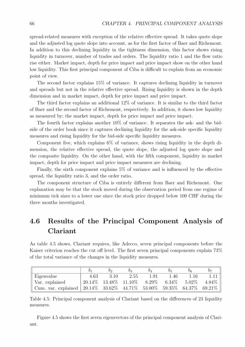
66 CHAPTER 4. PRINCIPAL COMPONENT ANALYSIS
spread-related measures with exception of the relative effective spread. It takes quote slope
and the adjusted log quote slope into account, as for the first factor of Baer and Richemont.
In addition to this declining liquidity in the tightness dimension, this factor shows rising
liquidity in turnover, number of trades and orders. The liquidity ratio 1 and the flow ratio
rise either. Market impact, depth for price impact and price impact show on the other hand
low liquidity. This first principal component of Ciba is difficult to explain from an economic
point of view.
The second factor explains 15% of variance. It captures declining liquidity in turnover
and spreads but not in the relative effective spread. Rising liquidity is shown in the depth
dimension and in market impact, depth for price impact and price impact.
The third factor explains an additional 12% of variance. It is similar to the third factor
of Baer and the second factor of Richemont, respectively. In addition, it shows low liquidity
as measured by; the market impact, depth for price impact and price impact.
The fourth factor explains another 10% of variance. It separates the ask- and the bid-
side of the order book since it captures declining liquidity for the ask-side specific liquidity
measures and rising liquidity for the bid-side specific liquidity measures.
Component five, which explains 6% of variance, shows rising liquidity in the depth di-
mension, the relative effective spread, the quote slope, the adjusted log quote slope and
the composite liquidity. On the other hand, with the fifth component, liquidity in market
impact, depth for price impact and price impact measures are declining.
Finally, the sixth component explains 5% of variance and is influenced by the effective
spread, the liquidity ratio 3, and the order ratio.
The component structure of Ciba is entirely different from Baer and Richemont. One
explanation may be that the stock moved during the observation period from one regime of
minimum tick sizes to a lower one since the stock price dropped below 100 CHF during the
three months investigated.
4.6 Results of the Principal Component Analysis of
Clariant
As table 4.5 shows, Clariant requires, like Adecco, seven principal components before the
Kaiser criterion reaches the cut off level. The first seven principal components explain 73%
of the total variance of the changes in the liquidity measures.
b1 b2 b3 b4 b5 b6 b7
Eigenvalue 4.63 3.10 2.55 1.91 1.46 1.16 1.11Var. explained 20.14% 13.48% 11.10% 8.29% 6.34% 5.02% 4.84%Cum. var. explained 20.14% 33.62% 44.71% 53.00% 59.35% 64.37% 69.21%
Table 4.5: Principal component analysis of Clariant based on the differences of 23 liquiditymeasures.
Figure 4.5 shows the first seven eigenvectors of the principal component analysis of Clari-
ant.
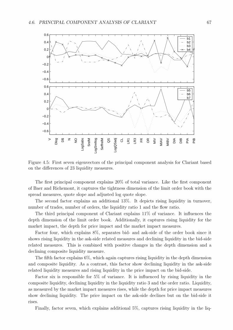
4.6. PRINCIPAL COMPONENT ANALYSIS OF CLARIANT 67
−0.6
−0.4
−0.2
0
0.2
0.4
0.6b1b2b3b4
−0.6
−0.4
−0.2
0
0.2
0.4
0.6
V
Dlo
g
D$ N
NO
LogS
abs
Sre
lM
LogS
rello
g
Sef
frel
M
QS
LogQ
Sad
j
CL
LR1
LR3
FR
OR
MIV
MIA
V
MIB
V
DIA
DIB
PIA
PIB
b5b6b7
Figure 4.5: First seven eigenvectors of the principal component analysis for Clariant basedon the differences of 23 liquidity measures.
The first principal component explains 20% of total variance. Like the first component
of Baer and Richemont, it captures the tightness dimension of the limit order book with the
spread measures, quote slope and adjusted log quote slope.
The second factor explains an additional 13%. It depicts rising liquidity in turnover,
number of trades, number of orders, the liquidity ratio 1 and the flow ratio.
The third principal component of Clariant explains 11% of variance. It influences the
depth dimension of the limit order book. Additionally, it captures rising liquidity for the
market impact, the depth for price impact and the market impact measures.
Factor four, which explains 8%, separates bid- and ask-side of the order book since it
shows rising liquidity in the ask-side related measures and declining liquidity in the bid-side
related measures. This is combined with positive changes in the depth dimension and a
declining composite liquidity measure.
The fifth factor explains 6%, which again captures rising liquidity in the depth dimension
and composite liquidity. As a contrast, this factor show declining liquidity in the ask-side
related liquidity measures and rising liquidity in the price impact on the bid-side.
Factor six is responsible for 5% of variance. It is influenced by rising liquidity in the
composite liquidity, declining liquidity in the liquidity ratio 3 and the order ratio. Liquidity,
as measured by the market impact measures rises, while the depth for price impact measures
show declining liquidity. The price impact on the ask-side declines but on the bid-side it
rises.
Finally, factor seven, which explains additional 5%, captures rising liquidity in the liq-
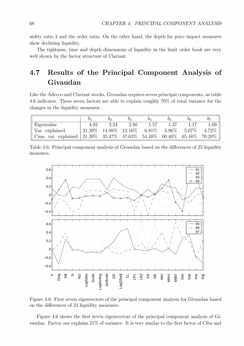
68 CHAPTER 4. PRINCIPAL COMPONENT ANALYSIS
uidity ratio 3 and the order ratio. On the other hand, the depth for price impact measures
show declining liquidity.
The tightness, time and depth dimensions of liquidity in the limit order book are very
well shown by the factor structure of Clariant.
4.7 Results of the Principal Component Analysis of
Givaudan
Like the Adecco and Clariant stocks, Givaudan requires seven principal components, as table
4.6 indicates. These seven factors are able to explain roughly 70% of total variance for the
changes in the liquidity measures.
b1 b2 b3 b4 b5 b6 b7
Eigenvalue 4.92 3.24 2.80 1.57 1.37 1.17 1.09Var. explained 21.39% 14.08% 12.16% 6.81% 5.96% 5.07% 4.72%Cum. var. explained 21.39% 35.47% 47.63% 54.48% 60.40% 65.48% 70.20%
Table 4.6: Principal component analysis of Givaudan based on the differences of 23 liquiditymeasures.
−0.4
−0.2
0
0.2
0.4
0.6 b1b2b3b4
−0.4
−0.2
0
0.2
0.4
0.6
V
Dlo
g
D$ N
NO
LogS
abs
Sre
lM
LogS
rello
g
Sef
frel
M
QS
LogQ
Sad
j
CL
LR1
LR3
FR
OR
MIV
MIA
V
MIB
V
DIA
DIB
PIA
PIB
b5b6b7
Figure 4.6: First seven eigenvectors of the principal component analysis for Givaudan basedon the differences of 23 liquidity measures.
Figure 4.6 shows the first seven eigenvectors of the principal component analysis of Gi-
vaudan. Factor one explains 21% of variance. It is very similar to the first factor of Ciba and
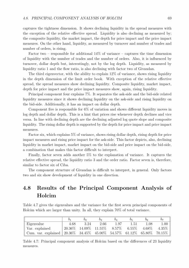
4.8. PRINCIPAL COMPONENT ANALYSIS OF HOLCIM 69
captures the tightness dimension. It shows declining liquidity in the spread measures with
the exception of the relative effective spread. Liquidity is also declining as measured by;
the composite liquidity, the market impact, the depth for price impact and the price impact
measures. On the other hand, liquidity, as measured by turnover and number of trades and
number of orders, is rising.
Factor two – responsible for additional 14% of variance – captures the time dimension
of liquidity with the number of trades and the number of orders. Also, it is influenced by
turnover, dollar depth but, interestingly, not by the log depth. Liquidity, as measured by
liquidity ratio 1 and the flow ratio, is also declining with factor two of Givaudan.
The third eigenvector, with the ability to explain 12% of variance, shows rising liquidity
in the depth dimension of the limit order book. With exception of the relative effective
spread, the spread measures show declining liquidity. Composite liquidity, market impact,
depth for price impact and the price impact measures show, again, rising liquidity.
Principal component four explains 7%. It separates the ask-side and the bid-side related
liquidity measures since it shows declining liquidity on the ask-side and rising liquidity on
the bid-side. Additionally, it has an impact on dollar depth.
Component five is responsible for 6% of variation and shows different liquidity moves in
log depth and dollar depth. This is a hint that prices rise whenever depth declines and vice
versa. In line with declining depth are the declining adjusted log quote slope and composite
liquidity. The rising dollar depth is supported by the depth for price impact and price impact
measures.
Factor six, which explains 5% of variance, shows rising dollar depth, rising depth for price
impact measures and rising price impact for the ask-side. This factor depicts, also, declining
liquidity in market impact, market impact on the bid-side and price impact on the bid-side,
a combination that makes this factor difficult to interpret.
Finally, factor seven adds another 5% to the explanation of variance. It captures the
relative effective spread, the liquidity ratio 3 and the order ratio. Factor seven is, therefore,
similar to factor six of Ciba.
The component structure of Givaudan is difficult to interpret, in general. Only factors
two and six show development of liquidity in one direction.
4.8 Results of the Principal Component Analysis of
Holcim
Table 4.7 gives the eigenvalues and the variance for the first seven principal components of
Holcim which are larger than unity. In all, they explain 70% of total variance.
b1 b2 b3 b4 b5 b6 b7
Eigenvalue 4.68 3.24 2.66 1.97 1.51 1.08 1.00Var. explained 20.36% 14.09% 11.55% 8.57% 6.55% 4.68% 4.35%Cum. var. explained 20.36% 34.45% 45.00% 54.57% 61.12% 65.80% 70.15%
Table 4.7: Principal component analysis of Holcim based on the differences of 23 liquiditymeasures.
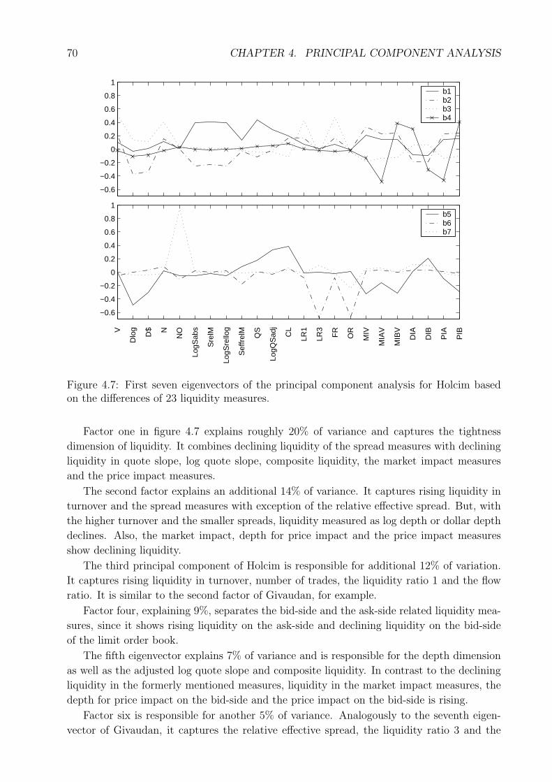
70 CHAPTER 4. PRINCIPAL COMPONENT ANALYSIS
−0.6
−0.4
−0.2
0
0.2
0.4
0.6
0.8
1b1b2b3b4
−0.6
−0.4
−0.2
0
0.2
0.4
0.6
0.8
1
V
Dlo
g
D$ N
NO
LogS
abs
Sre
lM
LogS
rello
g
Sef
frel
M
QS
LogQ
Sad
j
CL
LR1
LR3
FR
OR
MIV
MIA
V
MIB
V
DIA
DIB
PIA
PIB
b5b6b7
Figure 4.7: First seven eigenvectors of the principal component analysis for Holcim basedon the differences of 23 liquidity measures.
Factor one in figure 4.7 explains roughly 20% of variance and captures the tightness
dimension of liquidity. It combines declining liquidity of the spread measures with declining
liquidity in quote slope, log quote slope, composite liquidity, the market impact measures
and the price impact measures.
The second factor explains an additional 14% of variance. It captures rising liquidity in
turnover and the spread measures with exception of the relative effective spread. But, with
the higher turnover and the smaller spreads, liquidity measured as log depth or dollar depth
declines. Also, the market impact, depth for price impact and the price impact measures
show declining liquidity.
The third principal component of Holcim is responsible for additional 12% of variation.
It captures rising liquidity in turnover, number of trades, the liquidity ratio 1 and the flow
ratio. It is similar to the second factor of Givaudan, for example.
Factor four, explaining 9%, separates the bid-side and the ask-side related liquidity mea-
sures, since it shows rising liquidity on the ask-side and declining liquidity on the bid-side
of the limit order book.
The fifth eigenvector explains 7% of variance and is responsible for the depth dimension
as well as the adjusted log quote slope and composite liquidity. In contrast to the declining
liquidity in the formerly mentioned measures, liquidity in the market impact measures, the
depth for price impact on the bid-side and the price impact on the bid-side is rising.
Factor six is responsible for another 5% of variance. Analogously to the seventh eigen-
vector of Givaudan, it captures the relative effective spread, the liquidity ratio 3 and the
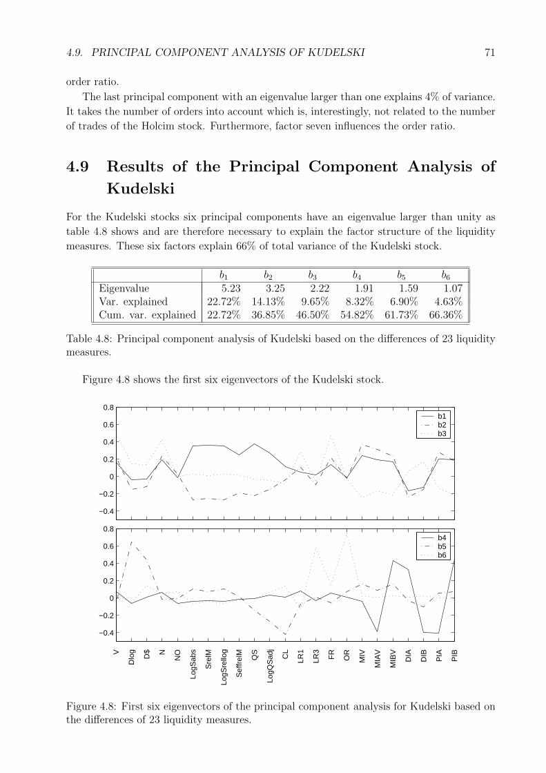
4.9. PRINCIPAL COMPONENT ANALYSIS OF KUDELSKI 71
order ratio.
The last principal component with an eigenvalue larger than one explains 4% of variance.
It takes the number of orders into account which is, interestingly, not related to the number
of trades of the Holcim stock. Furthermore, factor seven influences the order ratio.
4.9 Results of the Principal Component Analysis of
Kudelski
For the Kudelski stocks six principal components have an eigenvalue larger than unity as
table 4.8 shows and are therefore necessary to explain the factor structure of the liquidity
measures. These six factors explain 66% of total variance of the Kudelski stock.
b1 b2 b3 b4 b5 b6
Eigenvalue 5.23 3.25 2.22 1.91 1.59 1.07Var. explained 22.72% 14.13% 9.65% 8.32% 6.90% 4.63%Cum. var. explained 22.72% 36.85% 46.50% 54.82% 61.73% 66.36%
Table 4.8: Principal component analysis of Kudelski based on the differences of 23 liquiditymeasures.
Figure 4.8 shows the first six eigenvectors of the Kudelski stock.
−0.4
−0.2
0
0.2
0.4
0.6
0.8b1b2b3
−0.4
−0.2
0
0.2
0.4
0.6
0.8
V
Dlo
g
D$ N
NO
LogS
abs
Sre
lM
LogS
rello
g
Sef
frel
M
QS
LogQ
Sad
j
CL
LR1
LR3
FR
OR
MIV
MIA
V
MIB
V
DIA
DIB
PIA
PIB
b4b5b6
Figure 4.8: First six eigenvectors of the principal component analysis for Kudelski based onthe differences of 23 liquidity measures.
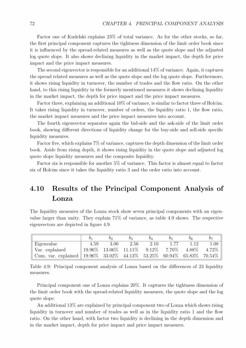
72 CHAPTER 4. PRINCIPAL COMPONENT ANALYSIS
Factor one of Kudelski explains 23% of total variance. As for the other stocks, so far,
the first principal component captures the tightness dimension of the limit order book since
it is influenced by the spread-related measures as well as the quote slope and the adjusted
log quote slope. It also shows declining liquidity in the market impact, the depth for price
impact and the price impact measures.
The second eigenvector is responsible for an additional 14% of variance. Again, it captures
the spread related measures as well as the quote slope and the log quote slope. Furthermore,
it shows rising liquidity in turnover, the number of trades and the flow ratio. On the other
hand, to this rising liquidity in the formerly mentioned measures it shows declining liquidity
in the market impact, the depth for price impact and the price impact measures.
Factor three, explaining an additional 10% of variance, is similar to factor three of Holcim.
It takes rising liquidity in turnover, number of orders, the liquidity ratio 1, the flow ratio,
the market impact measures and the price impact measures into account.
The fourth eigenvector separates again the bid-side and the ask-side of the limit order
book, showing different directions of liquidity change for the buy-side and sell-side specific
liquidity measures.
Factor five, which explains 7% of variance, captures the depth dimension of the limit order
book. Aside from rising depth, it shows rising liquidity in the quote slope and adjusted log
quote slope liquidity measures and the composite liquidity.
Factor six is responsible for another 5% of variance. This factor is almost equal to factor
six of Holcim since it takes the liquidity ratio 3 and the order ratio into account.
4.10 Results of the Principal Component Analysis of
Lonza
The liquidity measures of the Lonza stock show seven principal components with an eigen-
value larger than unity. They explain 71% of variance, as table 4.9 shows. The respective
eigenvectors are depicted in figure 4.9.
b1 b2 b3 b4 b5 b6 b7
Eigenvalue 4.59 3.00 2.56 2.10 1.77 1.12 1.08Var. explained 19.96% 13.06% 11.11% 9.12% 7.70% 4.88% 4.72%Cum. var. explained 19.96% 33.02% 44.13% 53.25% 60.94% 65.83% 70.54%
Table 4.9: Principal component analysis of Lonza based on the differences of 23 liquiditymeasures.
Principal component one of Lonza explains 20%. It captures the tightness dimension of
the limit order book with the spread-related liquidity measures, the quote slope and the log
quote slope.
An additional 13% are explained by principal component two of Lonza which shows rising
liquidity in turnover and number of trades as well as in the liquidity ratio 1 and the flow
ratio. On the other hand, with factor two liquidity is declining in the depth dimension and
in the market impact, depth for price impact and price impact measures.
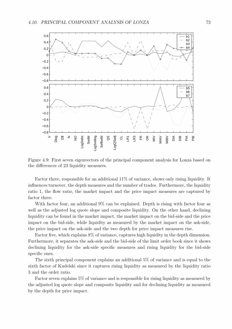
4.10. PRINCIPAL COMPONENT ANALYSIS OF LONZA 73
−0.8
−0.6
−0.4
−0.2
0
0.2
0.4
0.6 b1b2b3b4
−0.8
−0.6
−0.4
−0.2
0
0.2
0.4
0.6
V
Dlo
g
D$ N
NO
LogS
abs
Sre
lM
LogS
rello
g
Sef
frel
M
QS
LogQ
Sad
j
CL
LR1
LR3
FR
OR
MIV
MIA
V
MIB
V
DIA
DIB
PIA
PIB
b5b6b7
Figure 4.9: First seven eigenvectors of the principal component analysis for Lonza based onthe differences of 23 liquidity measures.
Factor three, responsible for an additional 11% of variance, shows only rising liquidity. It
influences turnover, the depth measures and the number of trades. Furthermore, the liquidity
ratio 1, the flow ratio, the market impact and the price impact measures are captured by
factor three.
With factor four, an additional 9% can be explained. Depth is rising with factor four as
well as the adjusted log quote slope and composite liquidity. On the other hand, declining
liquidity can be found in the market impact, the market impact on the bid-side and the price
impact on the bid-side, while liquidity as measured by the market impact on the ask-side,
the price impact on the ask-side and the two depth for price impact measures rise.
Factor five, which explains 8% of variance, captures high liquidity in the depth dimension.
Furthermore, it separates the ask-side and the bid-side of the limit order book since it shows
declining liquidity for the ask-side specific measures and rising liquidity for the bid-side
specific ones.
The sixth principal component explains an additional 5% of variance and is equal to the
sixth factor of Kudelski since it captures rising liquidity as measured by the liquidity ratio
3 and the order ratio.
Factor seven explains 5% of variance and is responsible for rising liquidity as measured by
the adjusted log quote slope and composite liquidity and for declining liquidity as measured
by the depth for price impact.
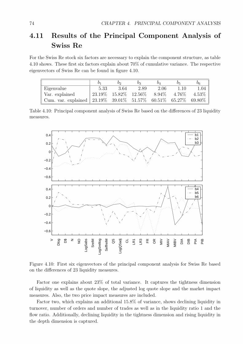
74 CHAPTER 4. PRINCIPAL COMPONENT ANALYSIS
4.11 Results of the Principal Component Analysis of
Swiss Re
For the Swiss Re stock six factors are necessary to explain the component structure, as table
4.10 shows. These first six factors explain about 70% of cumulative variance. The respective
eigenvectors of Swiss Re can be found in figure 4.10.
b1 b2 b3 b4 b5 b6
Eigenvalue 5.33 3.64 2.89 2.06 1.10 1.04Var. explained 23.19% 15.82% 12.56% 8.94% 4.76% 4.53%Cum. var. explained 23.19% 39.01% 51.57% 60.51% 65.27% 69.80%
Table 4.10: Principal component analysis of Swiss Re based on the differences of 23 liquiditymeasures.
−0.6
−0.4
−0.2
0
0.2
0.4 b1b2b3
−0.6
−0.4
−0.2
0
0.2
0.4
V
Dlo
g
D$ N
NO
LogS
abs
Sre
lM
LogS
rello
g
Sef
frel
M
QS
LogQ
Sad
j
CL
LR1
LR3
FR
OR
MIV
MIA
V
MIB
V
DIA
DIB
PIA
PIB
b4b5b6
Figure 4.10: First six eigenvectors of the principal component analysis for Swiss Re basedon the differences of 23 liquidity measures.
Factor one explains about 23% of total variance. It captures the tightness dimension
of liquidity as well as the quote slope, the adjusted log quote slope and the market impact
measures. Also, the two price impact measures are included.
Factor two, which explains an additional 15.8% of variance, shows declining liquidity in
turnover, number of orders and number of trades as well as in the liquidity ratio 1 and the
flow ratio. Additionally, declining liquidity in the tightness dimension and rising liquidity in
the depth dimension is captured.
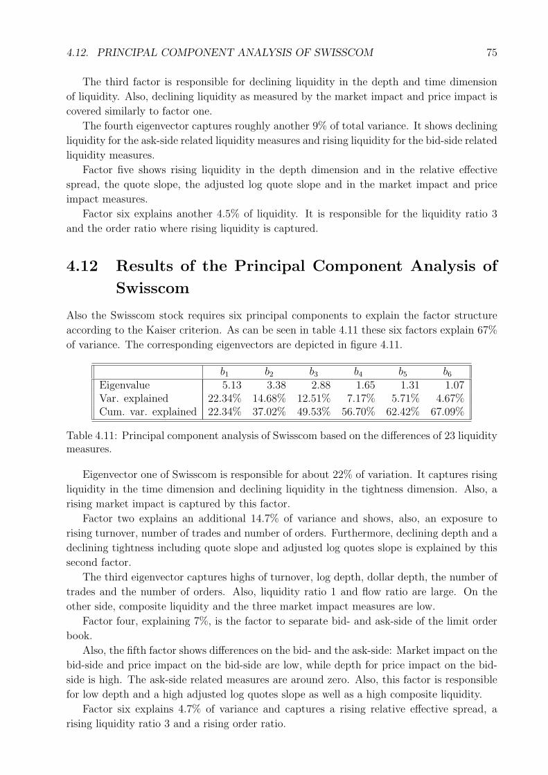
4.12. PRINCIPAL COMPONENT ANALYSIS OF SWISSCOM 75
The third factor is responsible for declining liquidity in the depth and time dimension
of liquidity. Also, declining liquidity as measured by the market impact and price impact is
covered similarly to factor one.
The fourth eigenvector captures roughly another 9% of total variance. It shows declining
liquidity for the ask-side related liquidity measures and rising liquidity for the bid-side related
liquidity measures.
Factor five shows rising liquidity in the depth dimension and in the relative effective
spread, the quote slope, the adjusted log quote slope and in the market impact and price
impact measures.
Factor six explains another 4.5% of liquidity. It is responsible for the liquidity ratio 3
and the order ratio where rising liquidity is captured.
4.12 Results of the Principal Component Analysis of
Swisscom
Also the Swisscom stock requires six principal components to explain the factor structure
according to the Kaiser criterion. As can be seen in table 4.11 these six factors explain 67%
of variance. The corresponding eigenvectors are depicted in figure 4.11.
b1 b2 b3 b4 b5 b6
Eigenvalue 5.13 3.38 2.88 1.65 1.31 1.07Var. explained 22.34% 14.68% 12.51% 7.17% 5.71% 4.67%Cum. var. explained 22.34% 37.02% 49.53% 56.70% 62.42% 67.09%
Table 4.11: Principal component analysis of Swisscom based on the differences of 23 liquiditymeasures.
Eigenvector one of Swisscom is responsible for about 22% of variation. It captures rising
liquidity in the time dimension and declining liquidity in the tightness dimension. Also, a
rising market impact is captured by this factor.
Factor two explains an additional 14.7% of variance and shows, also, an exposure to
rising turnover, number of trades and number of orders. Furthermore, declining depth and a
declining tightness including quote slope and adjusted log quotes slope is explained by this
second factor.
The third eigenvector captures highs of turnover, log depth, dollar depth, the number of
trades and the number of orders. Also, liquidity ratio 1 and flow ratio are large. On the
other side, composite liquidity and the three market impact measures are low.
Factor four, explaining 7%, is the factor to separate bid- and ask-side of the limit order
book.
Also, the fifth factor shows differences on the bid- and the ask-side: Market impact on the
bid-side and price impact on the bid-side are low, while depth for price impact on the bid-
side is high. The ask-side related measures are around zero. Also, this factor is responsible
for low depth and a high adjusted log quotes slope as well as a high composite liquidity.
Factor six explains 4.7% of variance and captures a rising relative effective spread, a
rising liquidity ratio 3 and a rising order ratio.
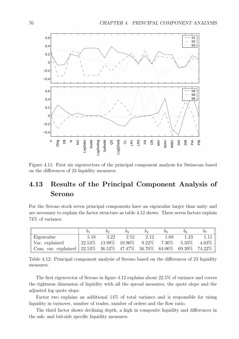
76 CHAPTER 4. PRINCIPAL COMPONENT ANALYSIS
−0.4
−0.2
0
0.2
0.4
0.6 b1b2b3
−0.4
−0.2
0
0.2
0.4
0.6
V
Dlo
g
D$ N
NO
LogS
abs
Sre
lM
LogS
rello
g
Sef
frel
M
QS
LogQ
Sad
j
CL
LR1
LR3
FR
OR
MIV
MIA
V
MIB
V
DIA
DIB
PIA
PIB
b4b5b6
Figure 4.11: First six eigenvectors of the principal component analysis for Swisscom basedon the differences of 23 liquidity measures.
4.13 Results of the Principal Component Analysis of
Serono
For the Serono stock seven principal components have an eigenvalue larger than unity and
are necessary to explain the factor structure as table 4.12 shows. These seven factors explain
74% of variance.
b1 b2 b3 b4 b5 b6 b7
Eigenvalue 5.18 3.22 2.52 2.12 1.69 1.23 1.11Var. explained 22.53% 13.98% 10.96% 9.22% 7.36% 5.33% 4.83%Cum. var. explained 22.53% 36.52% 47.47% 56.70% 64.06% 69.39% 74.22%
Table 4.12: Principal component analysis of Serono based on the differences of 23 liquiditymeasures.
The first eigenvector of Serono in figure 4.12 explains about 22.5% of variance and covers
the tightness dimension of liquidity with all the spread measures, the quote slope and the
adjusted log quote slope.
Factor two explains an additional 14% of total variance and is responsible for rising
liquidity in turnover, number of trades, number of orders and the flow ratio.
The third factor shows declining depth, a high in composite liquidity and differences in
the ask- and bid-side specific liquidity measures.
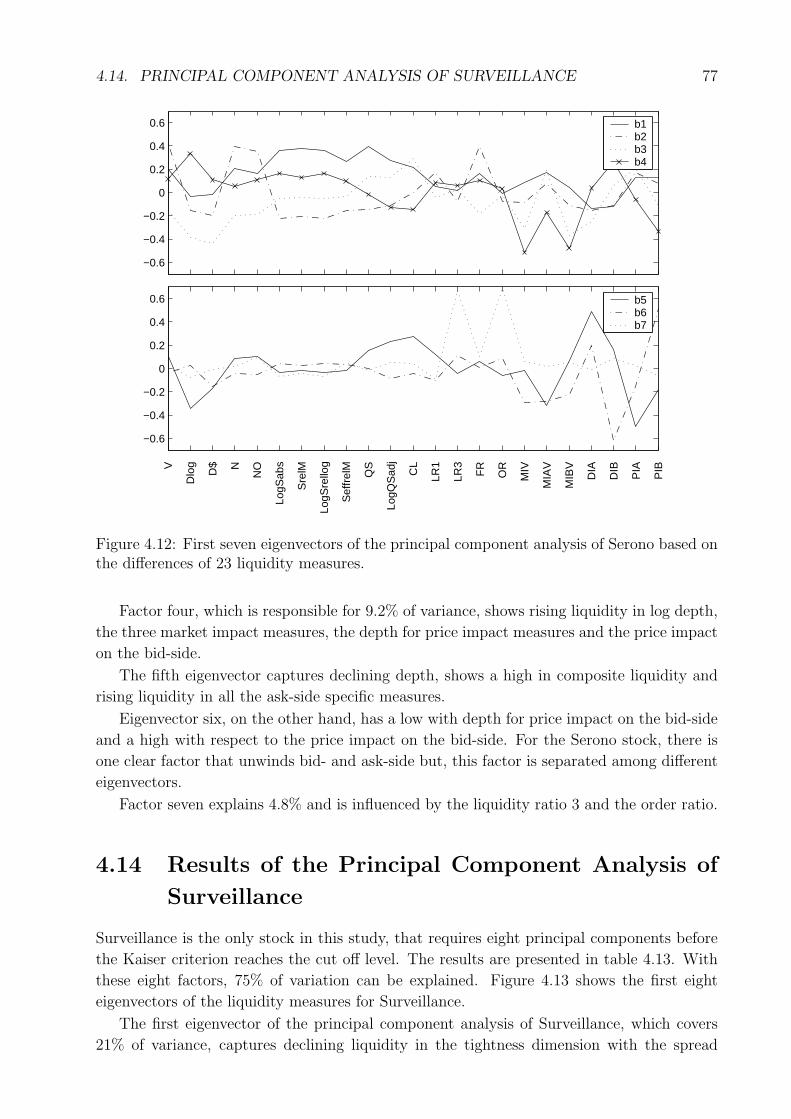
4.14. PRINCIPAL COMPONENT ANALYSIS OF SURVEILLANCE 77
−0.6
−0.4
−0.2
0
0.2
0.4
0.6 b1b2b3b4
−0.6
−0.4
−0.2
0
0.2
0.4
0.6
V
Dlo
g
D$ N
NO
LogS
abs
Sre
lM
LogS
rello
g
Sef
frel
M
QS
LogQ
Sad
j
CL
LR1
LR3
FR
OR
MIV
MIA
V
MIB
V
DIA
DIB
PIA
PIB
b5b6b7
Figure 4.12: First seven eigenvectors of the principal component analysis of Serono based onthe differences of 23 liquidity measures.
Factor four, which is responsible for 9.2% of variance, shows rising liquidity in log depth,
the three market impact measures, the depth for price impact measures and the price impact
on the bid-side.
The fifth eigenvector captures declining depth, shows a high in composite liquidity and
rising liquidity in all the ask-side specific measures.
Eigenvector six, on the other hand, has a low with depth for price impact on the bid-side
and a high with respect to the price impact on the bid-side. For the Serono stock, there is
one clear factor that unwinds bid- and ask-side but, this factor is separated among different
eigenvectors.
Factor seven explains 4.8% and is influenced by the liquidity ratio 3 and the order ratio.
4.14 Results of the Principal Component Analysis of
Surveillance
Surveillance is the only stock in this study, that requires eight principal components before
the Kaiser criterion reaches the cut off level. The results are presented in table 4.13. With
these eight factors, 75% of variation can be explained. Figure 4.13 shows the first eight
eigenvectors of the liquidity measures for Surveillance.
The first eigenvector of the principal component analysis of Surveillance, which covers
21% of variance, captures declining liquidity in the tightness dimension with the spread
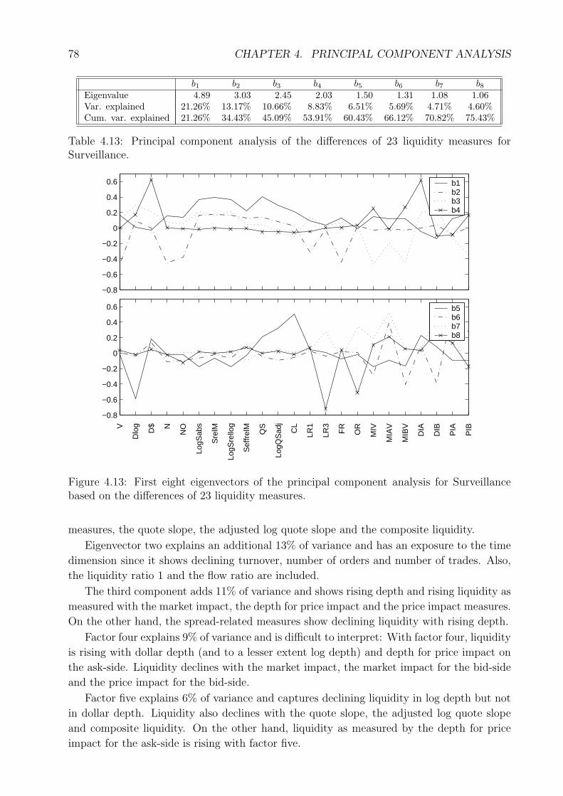
78 CHAPTER 4. PRINCIPAL COMPONENT ANALYSIS
b1 b2 b3 b4 b5 b6 b7 b8
Eigenvalue 4.89 3.03 2.45 2.03 1.50 1.31 1.08 1.06Var. explained 21.26% 13.17% 10.66% 8.83% 6.51% 5.69% 4.71% 4.60%Cum. var. explained 21.26% 34.43% 45.09% 53.91% 60.43% 66.12% 70.82% 75.43%
Table 4.13: Principal component analysis of the differences of 23 liquidity measures forSurveillance.
−0.8
−0.6
−0.4
−0.2
0
0.2
0.4
0.6 b1b2b3b4
−0.8
−0.6
−0.4
−0.2
0
0.2
0.4
0.6
V
Dlo
g
D$ N
NO
LogS
abs
Sre
lM
LogS
rello
g
Sef
frel
M
QS
LogQ
Sad
j
CL
LR1
LR3
FR
OR
MIV
MIA
V
MIB
V
DIA
DIB
PIA
PIB
b5b6b7b8
Figure 4.13: First eight eigenvectors of the principal component analysis for Surveillancebased on the differences of 23 liquidity measures.
measures, the quote slope, the adjusted log quote slope and the composite liquidity.
Eigenvector two explains an additional 13% of variance and has an exposure to the time
dimension since it shows declining turnover, number of orders and number of trades. Also,
the liquidity ratio 1 and the flow ratio are included.
The third component adds 11% of variance and shows rising depth and rising liquidity as
measured with the market impact, the depth for price impact and the price impact measures.
On the other hand, the spread-related measures show declining liquidity with rising depth.
Factor four explains 9% of variance and is difficult to interpret: With factor four, liquidity
is rising with dollar depth (and to a lesser extent log depth) and depth for price impact on
the ask-side. Liquidity declines with the market impact, the market impact for the bid-side
and the price impact for the bid-side.
Factor five explains 6% of variance and captures declining liquidity in log depth but not
in dollar depth. Liquidity also declines with the quote slope, the adjusted log quote slope
and composite liquidity. On the other hand, liquidity as measured by the depth for price
impact for the ask-side is rising with factor five.
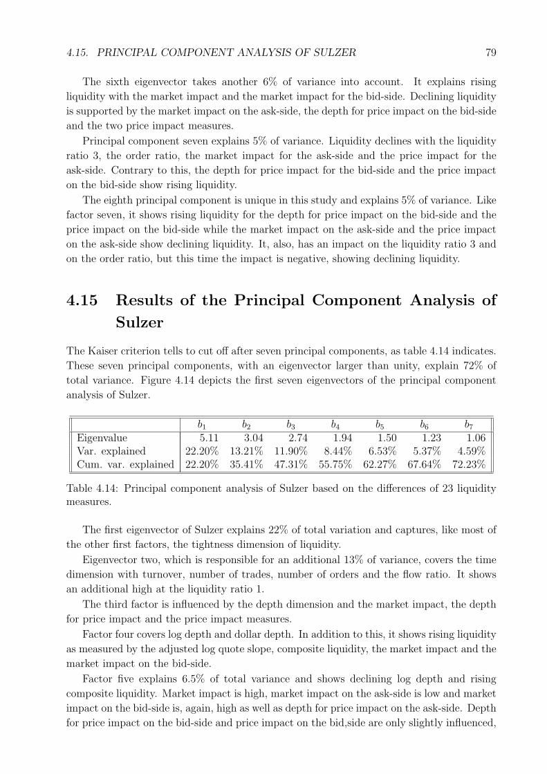
4.15. PRINCIPAL COMPONENT ANALYSIS OF SULZER 79
The sixth eigenvector takes another 6% of variance into account. It explains rising
liquidity with the market impact and the market impact for the bid-side. Declining liquidity
is supported by the market impact on the ask-side, the depth for price impact on the bid-side
and the two price impact measures.
Principal component seven explains 5% of variance. Liquidity declines with the liquidity
ratio 3, the order ratio, the market impact for the ask-side and the price impact for the
ask-side. Contrary to this, the depth for price impact for the bid-side and the price impact
on the bid-side show rising liquidity.
The eighth principal component is unique in this study and explains 5% of variance. Like
factor seven, it shows rising liquidity for the depth for price impact on the bid-side and the
price impact on the bid-side while the market impact on the ask-side and the price impact
on the ask-side show declining liquidity. It, also, has an impact on the liquidity ratio 3 and
on the order ratio, but this time the impact is negative, showing declining liquidity.
4.15 Results of the Principal Component Analysis of
Sulzer
The Kaiser criterion tells to cut off after seven principal components, as table 4.14 indicates.
These seven principal components, with an eigenvector larger than unity, explain 72% of
total variance. Figure 4.14 depicts the first seven eigenvectors of the principal component
analysis of Sulzer.
b1 b2 b3 b4 b5 b6 b7
Eigenvalue 5.11 3.04 2.74 1.94 1.50 1.23 1.06Var. explained 22.20% 13.21% 11.90% 8.44% 6.53% 5.37% 4.59%Cum. var. explained 22.20% 35.41% 47.31% 55.75% 62.27% 67.64% 72.23%
Table 4.14: Principal component analysis of Sulzer based on the differences of 23 liquiditymeasures.
The first eigenvector of Sulzer explains 22% of total variation and captures, like most of
the other first factors, the tightness dimension of liquidity.
Eigenvector two, which is responsible for an additional 13% of variance, covers the time
dimension with turnover, number of trades, number of orders and the flow ratio. It shows
an additional high at the liquidity ratio 1.
The third factor is influenced by the depth dimension and the market impact, the depth
for price impact and the price impact measures.
Factor four covers log depth and dollar depth. In addition to this, it shows rising liquidity
as measured by the adjusted log quote slope, composite liquidity, the market impact and the
market impact on the bid-side.
Factor five explains 6.5% of total variance and shows declining log depth and rising
composite liquidity. Market impact is high, market impact on the ask-side is low and market
impact on the bid-side is, again, high as well as depth for price impact on the ask-side. Depth
for price impact on the bid-side and price impact on the bid,side are only slightly influenced,
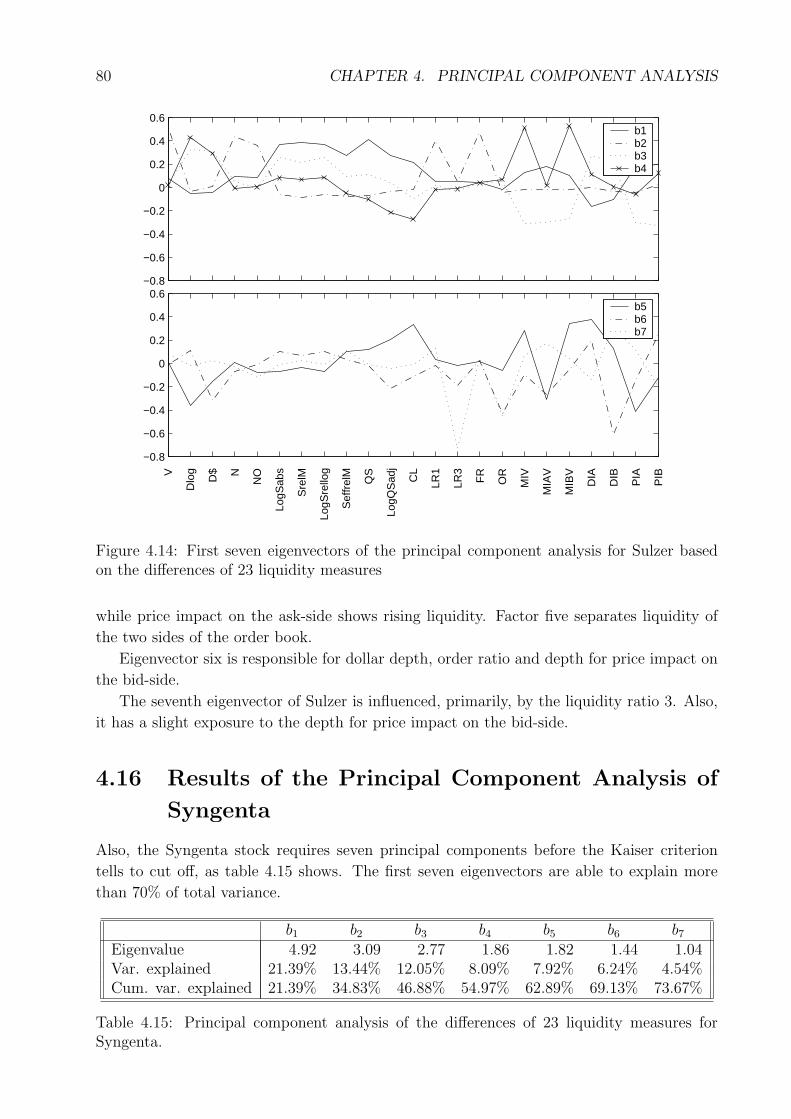
80 CHAPTER 4. PRINCIPAL COMPONENT ANALYSIS
−0.8
−0.6
−0.4
−0.2
0
0.2
0.4
0.6b1b2b3b4
−0.8
−0.6
−0.4
−0.2
0
0.2
0.4
0.6
V
Dlo
g
D$ N
NO
LogS
abs
Sre
lM
LogS
rello
g
Sef
frel
M
QS
LogQ
Sad
j
CL
LR1
LR3
FR
OR
MIV
MIA
V
MIB
V
DIA
DIB
PIA
PIB
b5b6b7
Figure 4.14: First seven eigenvectors of the principal component analysis for Sulzer basedon the differences of 23 liquidity measures
while price impact on the ask-side shows rising liquidity. Factor five separates liquidity of
the two sides of the order book.
Eigenvector six is responsible for dollar depth, order ratio and depth for price impact on
the bid-side.
The seventh eigenvector of Sulzer is influenced, primarily, by the liquidity ratio 3. Also,
it has a slight exposure to the depth for price impact on the bid-side.
4.16 Results of the Principal Component Analysis of
Syngenta
Also, the Syngenta stock requires seven principal components before the Kaiser criterion
tells to cut off, as table 4.15 shows. The first seven eigenvectors are able to explain more
than 70% of total variance.
b1 b2 b3 b4 b5 b6 b7
Eigenvalue 4.92 3.09 2.77 1.86 1.82 1.44 1.04Var. explained 21.39% 13.44% 12.05% 8.09% 7.92% 6.24% 4.54%Cum. var. explained 21.39% 34.83% 46.88% 54.97% 62.89% 69.13% 73.67%
Table 4.15: Principal component analysis of the differences of 23 liquidity measures forSyngenta.
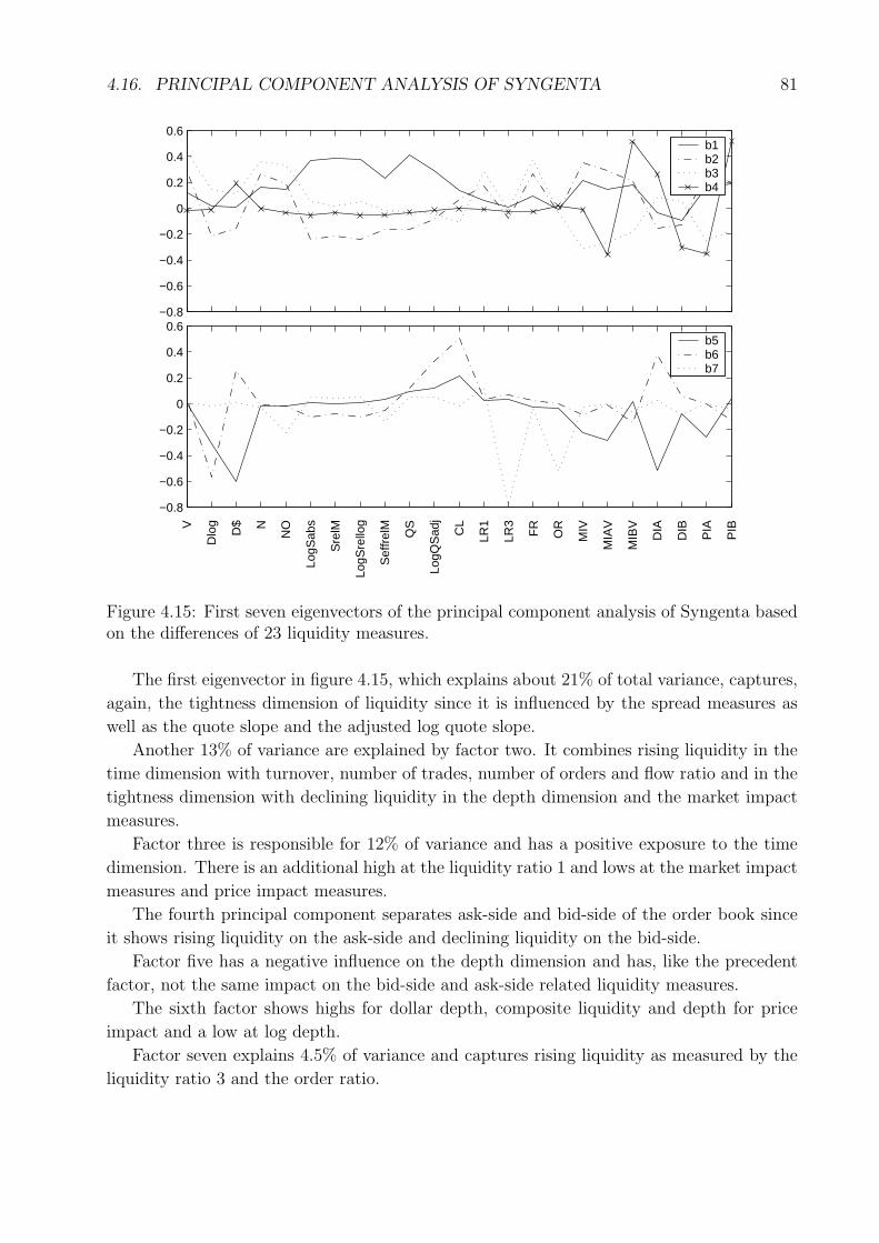
4.16. PRINCIPAL COMPONENT ANALYSIS OF SYNGENTA 81
−0.8
−0.6
−0.4
−0.2
0
0.2
0.4
0.6b1b2b3b4
−0.8
−0.6
−0.4
−0.2
0
0.2
0.4
0.6
V
Dlo
g
D$ N
NO
LogS
abs
Sre
lM
LogS
rello
g
Sef
frel
M
QS
LogQ
Sad
j
CL
LR1
LR3
FR
OR
MIV
MIA
V
MIB
V
DIA
DIB
PIA
PIB
b5b6b7
Figure 4.15: First seven eigenvectors of the principal component analysis of Syngenta basedon the differences of 23 liquidity measures.
The first eigenvector in figure 4.15, which explains about 21% of total variance, captures,
again, the tightness dimension of liquidity since it is influenced by the spread measures as
well as the quote slope and the adjusted log quote slope.
Another 13% of variance are explained by factor two. It combines rising liquidity in the
time dimension with turnover, number of trades, number of orders and flow ratio and in the
tightness dimension with declining liquidity in the depth dimension and the market impact
measures.
Factor three is responsible for 12% of variance and has a positive exposure to the time
dimension. There is an additional high at the liquidity ratio 1 and lows at the market impact
measures and price impact measures.
The fourth principal component separates ask-side and bid-side of the order book since
it shows rising liquidity on the ask-side and declining liquidity on the bid-side.
Factor five has a negative influence on the depth dimension and has, like the precedent
factor, not the same impact on the bid-side and ask-side related liquidity measures.
The sixth factor shows highs for dollar depth, composite liquidity and depth for price
impact and a low at log depth.
Factor seven explains 4.5% of variance and captures rising liquidity as measured by the
liquidity ratio 3 and the order ratio.
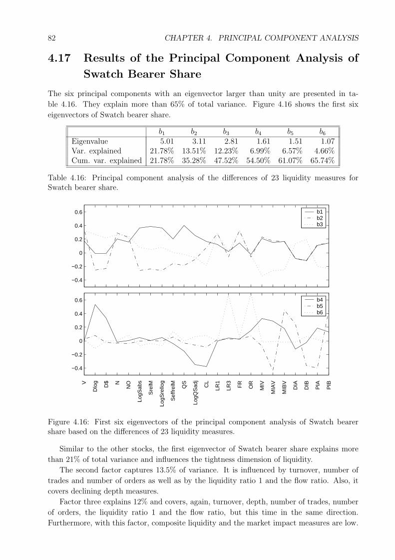
82 CHAPTER 4. PRINCIPAL COMPONENT ANALYSIS
4.17 Results of the Principal Component Analysis of
Swatch Bearer Share
The six principal components with an eigenvector larger than unity are presented in ta-
ble 4.16. They explain more than 65% of total variance. Figure 4.16 shows the first six
eigenvectors of Swatch bearer share.
b1 b2 b3 b4 b5 b6
Eigenvalue 5.01 3.11 2.81 1.61 1.51 1.07Var. explained 21.78% 13.51% 12.23% 6.99% 6.57% 4.66%Cum. var. explained 21.78% 35.28% 47.52% 54.50% 61.07% 65.74%
Table 4.16: Principal component analysis of the differences of 23 liquidity measures forSwatch bearer share.
−0.4
−0.2
0
0.2
0.4
0.6 b1b2b3
−0.4
−0.2
0
0.2
0.4
0.6
V
Dlo
g
D$ N
NO
LogS
abs
Sre
lM
LogS
rello
g
Sef
frel
M
QS
LogQ
Sad
j
CL
LR1
LR3
FR
OR
MIV
MIA
V
MIB
V
DIA
DIB
PIA
PIB
b4b5b6
Figure 4.16: First six eigenvectors of the principal component analysis of Swatch bearershare based on the differences of 23 liquidity measures.
Similar to the other stocks, the first eigenvector of Swatch bearer share explains more
than 21% of total variance and influences the tightness dimension of liquidity.
The second factor captures 13.5% of variance. It is influenced by turnover, number of
trades and number of orders as well as by the liquidity ratio 1 and the flow ratio. Also, it
covers declining depth measures.
Factor three explains 12% and covers, again, turnover, depth, number of trades, number
of orders, the liquidity ratio 1 and the flow ratio, but this time in the same direction.
Furthermore, with this factor, composite liquidity and the market impact measures are low.
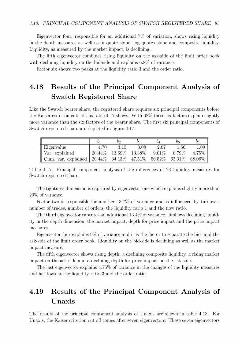
4.18. PRINCIPAL COMPONENT ANALYSIS OF SWATCH REGISTERED SHARE 83
Eigenvector four, responsible for an additional 7% of variation, shows rising liquidity
in the depth measures as well as in quote slope, log quotes slope and composite liquidity.
Liquidity, as measured by the market impact, is declining.
The fifth eigenvector combines rising liquidity on the ask-side of the limit order book
with declining liquidity on the bid-side and explains 6.8% of variance.
Factor six shows two peaks at the liquidity ratio 3 and the order ratio.
4.18 Results of the Principal Component Analysis of
Swatch Registered Share
Like the Swatch bearer share, the registered share requires six principal components before
the Kaiser criterion cuts off, as table 4.17 shows. With 68% these six factors explain slightly
more variance than the six factors of the bearer share. The first six principal components of
Swatch registered share are depicted in figure 4.17.
b1 b2 b3 b4 b5 b6
Eigenvalue 4.70 3.15 3.08 2.07 1.56 1.09Var. explained 20.44% 13.69% 13.38% 9.01% 6.79% 4.75%Cum. var. explained 20.44% 34.13% 47.51% 56.52% 63.31% 68.06%
Table 4.17: Principal component analysis of the differences of 23 liquidity measures forSwatch registered share.
The tightness dimension is captured by eigenvector one which explains slightly more than
20% of variance.
Factor two is responsible for another 13.7% of variance and is influenced by turnover,
number of trades, number of orders, the liquidity ratio 1 and the flow ratio.
The third eigenvector captures an additional 13.4% of variance. It shows declining liquid-
ity in the depth dimension, the market impact, depth for price impact and the price impact
measures.
Eigenvector four explains 9% of variance and it is the factor to separate the bid- and the
ask-side of the limit order book. Liquidity on the bid-side is declining as well as the market
impact measure.
The fifth eigenvector shows rising depth, a declining composite liquidity, a rising market
impact on the ask-side and a declining depth for price impact on the ask-side.
The last eigenvector explains 4.75% of variance in the changes of the liquidity measures
and has lows at the liquidity ratio 3 and the order ratio.
4.19 Results of the Principal Component Analysis of
Unaxis
The results of the principal component analysis of Unaxis are shown in table 4.18. For
Unaxis, the Kaiser criterion cut off comes after seven eigenvectors. These seven eigenvectors
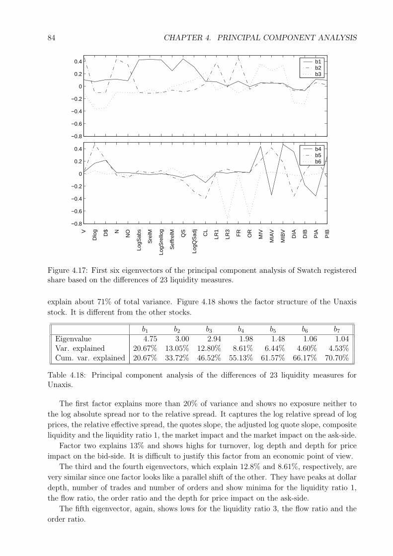
84 CHAPTER 4. PRINCIPAL COMPONENT ANALYSIS
−0.8
−0.6
−0.4
−0.2
0
0.2
0.4 b1b2b3
−0.8
−0.6
−0.4
−0.2
0
0.2
0.4
V
Dlo
g
D$ N
NO
LogS
abs
Sre
lM
LogS
rello
g
Sef
frel
M
QS
LogQ
Sad
j
CL
LR1
LR3
FR
OR
MIV
MIA
V
MIB
V
DIA
DIB
PIA
PIB
b4b5b6
Figure 4.17: First six eigenvectors of the principal component analysis of Swatch registeredshare based on the differences of 23 liquidity measures.
explain about 71% of total variance. Figure 4.18 shows the factor structure of the Unaxis
stock. It is different from the other stocks.
b1 b2 b3 b4 b5 b6 b7
Eigenvalue 4.75 3.00 2.94 1.98 1.48 1.06 1.04Var. explained 20.67% 13.05% 12.80% 8.61% 6.44% 4.60% 4.53%Cum. var. explained 20.67% 33.72% 46.52% 55.13% 61.57% 66.17% 70.70%
Table 4.18: Principal component analysis of the differences of 23 liquidity measures forUnaxis.
The first factor explains more than 20% of variance and shows no exposure neither to
the log absolute spread nor to the relative spread. It captures the log relative spread of log
prices, the relative effective spread, the quotes slope, the adjusted log quote slope, composite
liquidity and the liquidity ratio 1, the market impact and the market impact on the ask-side.
Factor two explains 13% and shows highs for turnover, log depth and depth for price
impact on the bid-side. It is difficult to justify this factor from an economic point of view.
The third and the fourth eigenvectors, which explain 12.8% and 8.61%, respectively, are
very similar since one factor looks like a parallel shift of the other. They have peaks at dollar
depth, number of trades and number of orders and show minima for the liquidity ratio 1,
the flow ratio, the order ratio and the depth for price impact on the ask-side.
The fifth eigenvector, again, shows lows for the liquidity ratio 3, the flow ratio and the
order ratio.
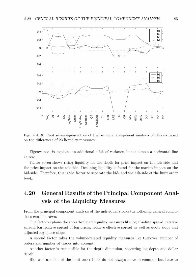
4.20. GENERAL RESULTS OF THE PRINCIPAL COMPONENT ANALYSIS 85
−0.4
−0.2
0
0.2
0.4 b1b2b3b4
−0.4
−0.2
0
0.2
0.4
V
Dlo
g
D$ N
NO
LogS
abs
Sre
lM
LogS
rello
g
Sef
frel
M
QS
LogQ
Sad
j
CL
LR1
LR3
FR
OR
MIV
MIA
V
MIB
V
DIA
DIB
PIA
PIB
b5b6b7
Figure 4.18: First seven eigenvectors of the principal component analysis of Unaxis basedon the differences of 23 liquidity measures.
Eigenvector six explains an additional 4.6% of variance, but is almost a horizontal line
at zero.
Factor seven shows rising liquidity for the depth for price impact on the ask-side and
the price impact on the ask-side. Declining liquidity is found for the market impact on the
bid-side. Therefore, this is the factor to separate the bid- and the ask-side of the limit order
book.
4.20 General Results of the Principal Component Anal-
ysis of the Liquidity Measures
From the principal component analysis of the individual stocks the following general conclu-
sions can be drawn:
One factor explains the spread-related liquidity measures like log absolute spread, relative
spread, log relative spread of log prices, relative effective spread as well as quote slope and
adjusted log quote slope.
A second factor takes the volume-related liquidity measures like turnover, number of
orders and number of trades into account.
Another factor is responsible for the depth dimension, capturing log depth and dollar
depth.
Bid- and ask-side of the limit order book do not always move in common but have to
86 CHAPTER 4. PRINCIPAL COMPONENT ANALYSIS
be split up in an ask-side specific and a bid-side specific liquidity. This finding is in line
with Irvine et al. (2000). In the principal component analysis this phenomenon may show
up either in one factor, covering rising liquidity on the ask-side and declining liquidity on
the bid-side or in two factors, influencing only the bid- or ask-side.
Somehow on their own stand the liquidity ratio 3 and the order ratio.
The results of the principal component analysis, therefore, suggest six dimensions of
liquidity which will be captured in the following chapters by the following liquidity measures:
1. Tightness
The tightness dimension can be described by the different spread measures. I chose
the relative spread with the mid-price in the denominator since it is comparable among
different stocks.
2. Time
The time dimension will be captured by the turnover since it is highly correlated with
the number of trades and is, again, comparable across different stocks.
3. Depth
For the same reason as above, dollar depth will describe the depth dimension of liq-
uidity.
4. Bid-side
The market impact for the bid-side is used to measure bid-side related liquidity since
it is easy to interpret and may be compared across different stocks.
5. Ask-side
Ask-side specific liquidity is measured by the market impact for the ask-side.
6. Resiliency
The resiliency dimension will be measured by the liquidity ratio 3 since it is easier to
interpret than the order ratio.
The dimensions of liquidity proposed in chapter 1 show up clearly in the results of the
principal component analysis. New is the separation of the bid-side and the ask-side of the
limit order book.

Part II
Predicting Liquidity
87


89
In the second part some ways to predict liquidity are investigated. Starting with the
sample of six liquidity measures determined at the end of part I, the next chapter will be
devoted to the lead-lag behavior of liquidity. In a vector autoregressive model the six liquidity
measures and returns will be included and the structure of these variables is analyzed for the
eighteen stocks. The last chapter 6 builds prediction models for the six liquidity measures
mentioned above which yield promising results.

90
Chapter 5
The Lead-Lag Behavior of Liquidity
Measures
In this chapter, the question is addressed whether there is a “normal” level of liquidity, and
whether there is mean-reversion in liquidity measures. This will yield possibilities to predict
liquidity, since a long term mean would be an estimate for liquidity. Coppejans et al. (2003)
detect mean-reversion in the measures “depth for price impact” which may be a general
result and could be adapted for other liquidity measures.
There may also be persistence in liquidity: A period of high liquidity tends to be followed
by another of high liquidity and the same holds for low liquidity. Chan et al. (2002) describe
positive autocorrelation among net-trade volumes in the stock market.
Engle & Lange (2001) show the net-directional-volume to be a function of magnitude
and timing of current and lagged transaction flows. The spread preceding a price-duration
is negatively related to V NET .
The lead-lag behavior of liquidity measures is investigated further using a vector au-
toregressive model as described, for example in Stier (2001). This will yield estimates for
the influence of lagged liquidity measures on the liquidity in time t, and is, therefore, an
approach that may lead to promising results in predicting liquidity.
5.1 Autocorrelation in Liquidity Measures and Returns
For the theory of autocorrelations see e.g. Hamilton (1994). The autocorrelation τ of the
change in the liquidity measure dm at lag k is estimated as
τk =
T∑t=k+1
(dmt − dm) · (dmt−k − dm)
T∑t=1
(dmt − dm)2
. (5.1)
91
92 CHAPTER 5. THE LEAD-LAG BEHAVIOR
With the Ljung-Box test, the autocorrelations are tested for their significance. The
Q-statistic for lag k is calculated as
Qk = T · (T + 2) ·k∑
j=1
τ 2j
T − j. (5.2)
Under the null hypothesis of no autocorrelation up to lag k, Q is asymptotically distributed
as a χ2 with k degrees of freedom, according to Ljung & Box (1978).
All the differences in liquidity measures show negative and significant autocorrelation at
lag 1. Afterwards the autocorrelation drops sharply to about zero which is a sign that the
differences in liquidity measures obey a moving-average process of order 1.
The partial autocorrelation ρ at lag k is approximated recursively, in line with Box &
Jenkins (1976), by
ρk =
τ1 for k = 1
τk−k−1∑j=1
ρk−1,j ·τk−j
1−k−1∑j=1
ρk−1,j ·τk−j
for k > 1. (5.3)
and
ρk,j = ρk−1,j − ρk · ρk−1,k−j. (5.4)
Since the partial autocorrelations of the differences for all liquidity measures gradually ap-
proach zero, they follow a moving average process.
For the returns, the picture is similar: seventeen stocks show slightly negative but signifi-
cant autocorrelations at lag one. The partial autocorrelations are dying out, and the returns
follow a moving average process. Only for Adecco is no autocorrelation in returns observed.
5.2 The Vector Autoregressive Model
There are several studies employing the vector autoregressive model in the context of market
microstructure: George & Hwang (1998) e.g. use a vector autoregressive model to evaluate
daytime and overnight order flows with its respective returns, and Trapletti, Geyer & Leisch
(2002) try to forecast exchange rates using a vector autoregressive model. Chung, Han &
Tse (1996) examine the interrelation between NYSE, AMEX and NASDAQ markets with a
VAR model and describe the methodology extensively.
An n-dimensional vector-autoregressive model of order p (VAR(p)-process) is defined
according to Hamilton (1994) or Stier (2001) as:
xt = c + Φ1 · xt−1 + Φ2 · xt−2 + ... + Φp · xt−p + εt (5.5)
In our case, the vector xt consists of the changes in the six liquidity measures and returns
in time t. n is therefore equal to seven. xt is regressed upon its own lagged variables.
Φi(i = 1, 2, ..., p) denotes the (n×n)-parameter matrices with Φp 6= 0. c is an (n× 1) vector
of constants which may be a vector of zeros. εt is a vector of white noise.
To determine the appropriate number of lags (p) to include, the Schwarz information
5.3. RESULTS OF THE VAR MODEL FOR ADECCO 93
criterion (SIC) by Schwarz (1978) was employed. It is given by:
SIC = −2 · ( l
T) + k · log(T )
T(5.6)
l is the value of the log likelihood function with the k parameters estimated from the T
observations. l is given by
l = −T ·M2
· (1 + ln(2 · π))− T
2· ln |Ω| (5.7)
M is the number of equations and
|Ω| = det(∑
i
εε′
T). (5.8)
The Schwarz information criterion reaches its maximum for all stocks at seven lags. There-
fore, seven lags are included in the vector autoregressive model.
5.3 Results of the VAR model for Adecco
Table 5.1 presents the results of the vector autoregressive model for Adecco. As described
above, the first differences of six liquidity measures are included as well as returns. The model
includes seven lags since there the Schwarz information criterion reaches its maximum.
The relative spread depends on all its own lagged expressions negatively and the coeffi-
cients are highly significant. Therefore, rising spreads are followed by declining ones. This
result holds for all liquidity measures: The vector autoregressive model shows a significantly
negative impact of the changes in t− 7 until t− 1 on the liquidity measure in t. The relative
spread is positively influenced by changes in turnover. There is significance for lags one to
three, and seven. Rising liquidity, as measured by turnover, leads to lower liquidity measured
by the spread. Between dollar depth and the spread there is no significant relation. The
relative spread is positively influenced by the market impacts on the bid- and the ask-side.
For the ask-side the impact is significant up to lag five (at a level of at least 5%), whereas on
the bid-side only the first two lags are significant. The liquidity ratio 3 has only a slightly
significant impact on the lag seven which is negative. The first lag of the returns influences
the relative spread significantly: A declining stock price inflates the spread. At the lag seven
this relation is significantly positive. The constant is not significantly different from zero
which holds for the whole VAR system.
Turnover is not significantly influenced by the relative spread. For dollar depth there is
a slightly positive relation for the first lag. Turnover depends strongly on the lagged market
impacts: A negative significance on a level of at least 5% is recognized for lags up to five
on the ask-side and up to six on the bid-side. The liquidity ratio 3 influences only slightly
turnover on lag two. The returns are negatively related on lags one to five but significant
are only the values for lag two and five on a level of 10% and 5%, respectively.
Dollar depth in time t is not influenced by the lagged relative spreads. Therefore, there
is no interrelation between the tightness and the depth dimension of liquidity. Turnover
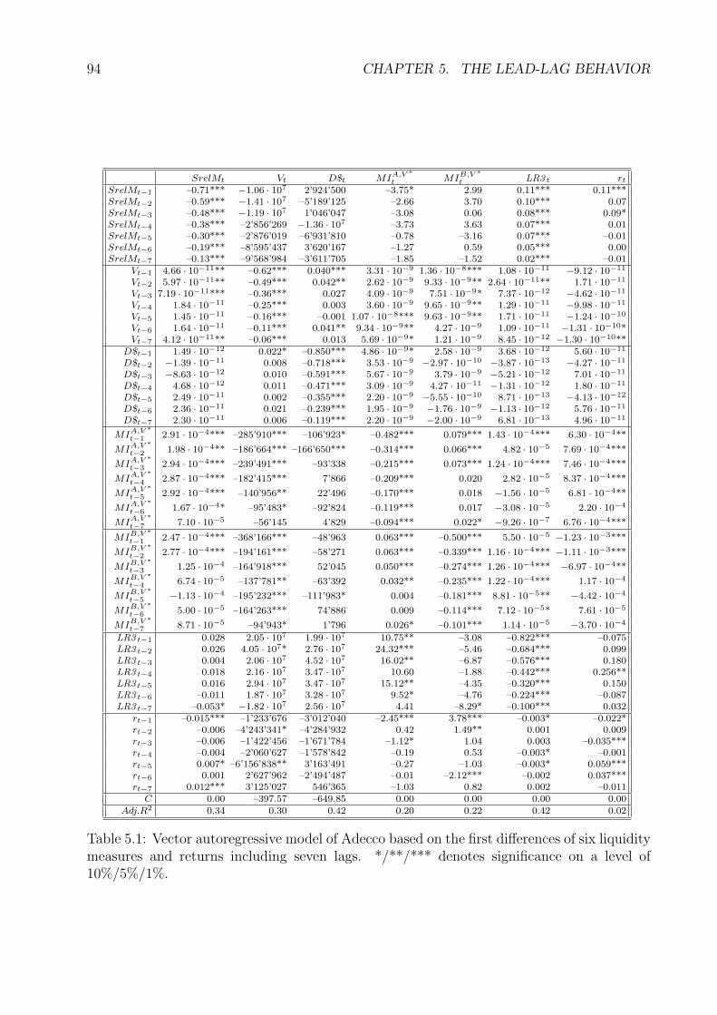
94 CHAPTER 5. THE LEAD-LAG BEHAVIOR
SrelMt Vt D$t MIA,V ∗t MIB,V ∗
t LR3 t rt
SrelMt−1 –0.71*** −1.06 · 107 2’924’500 –3.75* 2.99 0.11*** 0.11***SrelMt−2 –0.59*** −1.41 · 107 –5’189’125 –2.66 3.70 0.10*** 0.07SrelMt−3 –0.48*** −1.19 · 107 1’046’047 –3.08 0.06 0.08*** 0.09*SrelMt−4 –0.38*** –2’856’269 −1.36 · 107 –3.73 3.63 0.07*** 0.01SrelMt−5 –0.30*** –2’876’019 –6’931’810 –0.78 –3.16 0.07*** –0.01SrelMt−6 –0.19*** –8’595’437 3’620’167 –1.27 0.59 0.05*** 0.00SrelMt−7 –0.13*** –9’568’984 –3’611’705 –1.85 –1.52 0.02*** –0.01
Vt−1 4.66 · 10−11** –0.62*** 0.040*** 3.31 · 10−9 1.36 · 10−8*** 1.08 · 10−11 −9.12 · 10−11
Vt−2 5.97 · 10−11** –0.49*** 0.042** 2.62 · 10−9 9.33 · 10−9** 2.64 · 10−11** 1.71 · 10−11
Vt−3 7.19 · 10−11*** –0.36*** 0.027 4.09 · 10−9 7.51 · 10−9* 7.37 · 10−12 −4.62 · 10−11
Vt−4 1.84 · 10−11 –0.25*** 0.003 3.60 · 10−9 9.65 · 10−9** 1.29 · 10−11 −9.98 · 10−11
Vt−5 1.45 · 10−11 –0.16*** –0.001 1.07 · 10−8*** 9.63 · 10−9** 1.71 · 10−11 −1.24 · 10−10
Vt−6 1.64 · 10−11 –0.11*** 0.041** 9.34 · 10−9** 4.27 · 10−9 1.09 · 10−11 −1.31 · 10−10*Vt−7 4.12 · 10−11** –0.06*** 0.013 5.69 · 10−9* 1.21 · 10−9 8.45 · 10−12 −1.30 · 10−10**
D$t−1 1.49 · 10−12 0.022* –0.850*** 4.86 · 10−9* 2.58 · 10−9 3.68 · 10−12 5.60 · 10−11
D$t−2 −1.39 · 10−11 0.008 –0.718*** 3.53 · 10−9 −2.97 · 10−10 −3.87 · 10−13 −4.27 · 10−11
D$t−3 −8.63 · 10−12 0.010 –0.591*** 5.67 · 10−9 3.79 · 10−9 −5.21 · 10−12 7.01 · 10−11
D$t−4 4.68 · 10−12 0.011 –0.471*** 3.09 · 10−9 4.27 · 10−11 −1.31 · 10−12 1.80 · 10−11
D$t−5 2.49 · 10−11 0.002 –0.355*** 2.20 · 10−9 −5.55 · 10−10 8.71 · 10−13 −4.13 · 10−12
D$t−6 2.36 · 10−11 0.021 –0.239*** 1.95 · 10−9 −1.76 · 10−9 −1.13 · 10−12 5.76 · 10−11
D$t−7 2.30 · 10−11 0.006 –0.119*** 2.20 · 10−9 −2.00 · 10−9 6.81 · 10−13 4.96 · 10−11
MIA,V ∗t−1 2.91 · 10−4*** –285’910*** –106’923* –0.482*** 0.079*** 1.43 · 10−4*** 6.30 · 10−4**
MIA,V ∗t−2 1.98 · 10−4** –186’664*** –166’650*** –0.314*** 0.066*** 4.82 · 10−5 7.69 · 10−4***
MIA,V ∗t−3 2.94 · 10−4*** –239’491*** –93’338 –0.215*** 0.073*** 1.24 · 10−4*** 7.46 · 10−4***
MIA,V ∗t−4 2.87 · 10−4*** –182’415*** 7’866 –0.209*** 0.020 2.82 · 10−5 8.37 · 10−4***
MIA,V ∗t−5 2.92 · 10−4*** –140’956** 22’496 –0.170*** 0.018 −1.56 · 10−5 6.81 · 10−4**
MIA,V ∗t−6 1.67 · 10−4* –95’483* –92’824 –0.119*** 0.017 −3.08 · 10−5 2.20 · 10−4
MIA,V ∗t−7 7.10 · 10−5 –56’145 4’829 –0.094*** 0.022* −9.26 · 10−7 6.76 · 10−4***
MIB,V ∗t−1 2.47 · 10−4*** –368’166*** –48’963 0.063*** –0.500*** 5.50 · 10−5 −1.23 · 10−3***
MIB,V ∗t−2 2.77 · 10−4*** –194’161*** –58’271 0.063*** –0.339*** 1.16 · 10−4*** −1.11 · 10−3***
MIB,V ∗t−3 1.25 · 10−4 –164’918*** 52’045 0.050*** –0.274*** 1.26 · 10−4*** −6.97 · 10−4**
MIB,V ∗t−4 6.74 · 10−5 –137’781** –63’392 0.032** –0.235*** 1.22 · 10−4*** 1.17 · 10−4
MIB,V ∗t−5 −1.13 · 10−4 –195’232*** –111’983* 0.004 –0.181*** 8.81 · 10−5** −4.42 · 10−4
MIB,V ∗t−6 5.00 · 10−5 –164’263*** 74’886 0.009 –0.114*** 7.12 · 10−5* 7.61 · 10−5
MIB,V ∗t−7 8.71 · 10−5 –94’943* 1’796 0.026* –0.101*** 1.14 · 10−5 −3.70 · 10−4
LR3 t−1 0.028 2.05 · 107 1.99 · 107 10.75** –3.08 –0.822*** –0.075LR3 t−2 0.026 4.05 · 107* 2.76 · 107 24.32*** –5.46 –0.684*** 0.099LR3 t−3 0.004 2.06 · 107 4.52 · 107 16.02** –6.87 –0.576*** 0.180LR3 t−4 0.018 2.16 · 107 3.47 · 107 10.60 –1.88 –0.442*** 0.256**LR3 t−5 0.016 2.94 · 107 3.47 · 107 15.12** –4.35 –0.320*** 0.150LR3 t−6 –0.011 1.87 · 107 3.28 · 107 9.52* –4.76 –0.224*** –0.087LR3 t−7 –0.053* −1.82 · 107 2.56 · 107 4.41 –8.29* –0.100*** 0.032
rt−1 –0.015*** –1’233’676 –3’012’040 –2.45*** 3.78*** –0.003* –0.022*rt−2 –0.006 –4’243’341* –4’284’932 0.42 1.49** 0.001 0.009rt−3 –0.006 –1’422’456 –1’671’784 –1.12* 1.04 0.003 –0.035***rt−4 –0.004 –2’060’627 –1’578’842 –0.19 0.53 –0.003* –0.001rt−5 0.007* –6’156’838** 3’163’491 –0.27 –1.03 –0.003* 0.059***rt−6 0.001 2’627’962 –2’494’487 –0.01 –2.12*** –0.002 0.037***rt−7 0.012*** 3’125’027 546’365 –1.03 0.82 0.002 –0.011
C 0.00 –397.57 –649.85 0.00 0.00 0.00 0.00Adj.R2 0.34 0.30 0.42 0.20 0.22 0.42 0.02
Table 5.1: Vector autoregressive model of Adecco based on the first differences of six liquiditymeasures and returns including seven lags. */**/*** denotes significance on a level of10%/5%/1%.
5.3. RESULTS OF THE VAR MODEL FOR ADECCO 95
influences dollar depth significantly positively on lags one, two and six. Most of the market
impact measures are negatively related to dollar depth which is an intuitive result. When
market impact declines the order book becomes thicker and depth rises. On a 1% significance
level the effect shows up for the market impact on the ask-side on lag two and on a 10%
significance level for the ask-side on lag one and on the bid-side on lag five. The lagged
liquidity ratio 3 and the lagged returns show no explanatory power with respect to dollar
depth.
The relative spread on lag 1 influences the market impact on the ask-side only slightly
negatively. Turnover and market impact on the ask-side are positively related as for turnover
and spread. Higher liquidity as measured by turnover is followed by lower liquidity as
measured by market impact, but the effect is only significant for lags five to seven. Dollar
depth shows only a positive lagged influence on market impact on the ask-side for lag one.
Market impact on the bid-side seems to have a large positive effect on market impact on the
ask-side: On a significance level of at least 5% the first four lags are able to predict liquidity
on the other side of the order book. Lagged liquidity as measured by the liquidity ratio 3
and market impact are also positively correlated. Significant values show up for lags one to
three, five and six. Rising stock prices are mostly followed by declining market impacts as
lags one and three show.
The relative spread has no predictive power to market impact on the bid-side. Rising
turnover influences the market impact on the bid-side positively. The effect seems to be
complementary to the relation of lagged turnover and market impact on the ask-side: The
first five lags of turnover have an effect on market impact on the bid-side, while the effect on
market impact on the ask-side is significant for lags five to seven. There is no effect of lagged
dollar depth on market impact on the bid-side. Market impact on the ask-side on lags one
to three influences market impact on the bid-side significantly. The lagged liquidity ratio
3 shows almost no predictive power with respect to market impact on the bid-side. While
the impact of returns on market impact on the ask-side was mostly negative, it is mostly
positive for market impact on the bid-side. Significantly positive values show up for lags one
and two while lag six is significantly negative.
The liquidity ratio 3 is positively influenced by the relative spread for all lags. Turnover
has only predictive power on lag two; it is also positive. There is no influence of lagged dollar
depth on the liquidity ratio 3. Market impact on the ask-side shows for lags one and three a
significantly positive relation to the liquidity ratio 3. In contrast to this, significant lags for
the effect to market impact on the bid-side on the liquidity ratio 3 are from two to six. The
effect of lagged returns to the liquidity ratio 3 is almost zero. It is only slightly significant
on lags one, four and five.
A high spread is usually followed by a high return as the relation between relative spread
and log returns show. The impact of turnover on returns is mostly negative, and is significant
for lags six and seven. There is no impact of dollar depth on returns. The relation of market
impact on the ask-side on returns is always positive and significant for almost all lags. In
contrast to this, market impact on the bid-side is negatively related to returns; significantly
for lags one to three. This means that low liquidity on the ask-side is usually followed by
rising stock prices while low liquidity on the bid-side is followed by declining stock prices
– an economically intuitive result. Finally, the interrelation of lagged returns on return in
96 CHAPTER 5. THE LEAD-LAG BEHAVIOR
time t is ambiguous: It is significantly negative on lags one and three while it is significantly
positive on lags five and six.
The adjusted R2 values vary between 42% for the explanation of the dollar depth and
the liquidity ratio 3 and 2% for the regression of returns.
5.4 Results of the VAR model for Baer
Table 5.2 presents the results of the vector autoregressive model of Baer.
As for the Adecco stock, all the liquidity measures of Baer are strongly negatively influ-
enced by its own changes at all lags.
For the Baer stock the relative spread depends significantly positively on turnover for lags
three to five and seven. Turnover on other lags yields no prediction for the relative spread.
Dollar depth has a significantly positive impact on the relative spread on lags from two to
seven, which is a different result compared to the Adecco stock. The first lag of market
impact on the ask-side has a slightly positive impact on the relative spread. Lags four and
five have a significantly negative impact on the spread. All the lags of market impact on the
bid-side have a positive influence on the relative spread. There is significance for lags one and
three to six. Lags one to three of the liquidity ratio 3 have a significantly positive influence
on the relative spread while the impact of the seventh lag is significantly negative. The
lagged returns are mostly negatively related to the relative spread. The impact is significant
for lags three, five and six.
Only the relative spread of lag two influences turnover slightly. Lagged dollar depth is
positively related to turnover and is significant on lags two, three, five and six. Similar to
the Adecco stock, lagged market impact on the ask-side has a negative impact on turnover;
significantly for lags one to three. However, market impact on the bid-side is different: Only
the coefficient of lag six of market impact on the bid-side is slightly significant. There is no
impact of the lagged liquidity ratio 3 and of lagged returns on turnover.
The first two lags of the relative spread influence dollar depth significantly negatively.
Therefore, rising depth leads to higher spreads but, in turn, this effects again lower depth.
Higher turnover leads to lower depth, sometimes significantly, as the results in table 5.2 show.
Of the lagged differences of the market impact measures, only market impact on the ask-side
for lag five and market impact on the bid-side for lag four influence dollar depth significantly
negatively. The liquidity ratio 3 shows no impact on dollar depth at all. The significant
coefficients of lagged returns all show a positive relation to depth, while for Adecco there
was no significance.
As for the Adecco stock, the relative spread for Baer influences market impact on the ask-
side negatively. The effect is significant for lags one, three, four and six. Lagged turnover and
dollar depth are not related to market impact on the ask-side. Lagged market impact on the
bid-side has an ambiguous influence on market impact on the ask-side: For the first two lags
it is negative and significant while for lags four to seven it is positive and significant. There
is almost no impact of the liquidity ratio 3 on market impact on the ask-side. Lagged returns
are negatively correlated to market impact on the ask-side. For Baer there is significance for
lags two to five and seven.
While the effect of the lagged spreads was negative on the market impact on the ask-side
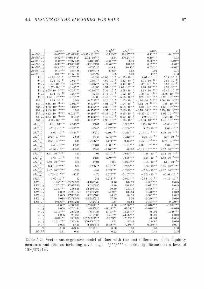
5.4. RESULTS OF THE VAR MODEL FOR BAER 97
SrelMt Vt D$t MIA,V ∗t MIB,V ∗
t LR3 t rt
SrelMt−1 –0.65*** –2’401’633 −3.47 · 107*** –35.45** 314.97*** 0.12*** –0.12***SrelMt−2 –0.52*** 5’086’341* −2.02 · 106** –2.34 336.24*** 0.10*** –0.03SrelMt−3 –0.41*** –3’827’538 −1.10 · 106 –61.83*** 11.79 0.09*** –0.10**SrelMt−4 –0.33*** –4’760’847 –9’816’197 –58.69*** 101.02 0.07*** –0.07*SrelMt−5 –0.24*** –579’185 –774’423 –19.11 180.85* 0.05*** –0.07*SrelMt−6 –0.14*** –983’488 –4’407’978 –29.66* –5.68 0.02 0.04SrelMt−7 –0.08*** 1’347’119 –653’227 1.68 –14.00 0.02** 0.03
Vt−1 −4.01 · 10−11 –0.75*** –0.054 −6.06 · 10−8 −1.15 · 10−7 6.07 · 10−11 5.18 · 10−11
Vt−2 7.25 · 10−11 –0.61*** –0.104** 4.69 · 10−8 3.32 · 10−7 1.03 · 10−10* 2.61 · 10−11
Vt−3 1.54 · 10−10* –0.53*** –0.107** 2.74 · 10−8 4.43 · 10−7 1.38 · 10−10** 8.87 · 10−11
Vt−4 1.57 · 10−10* –0.42*** –0.08* 8.97 · 10−8 9.61 · 10−7* 1.18 · 10−10* 4.98 · 10−11
Vt−5 2.55 · 10−10*** –0.27*** –0.105** 7.34 · 10−8 2.58 · 10−7 1.13 · 10−10* −2.40 · 10−10
Vt−6 1.14 · 10−10 –0.20*** –0.055 −1.74 · 10−9 1.92 · 10−7 1.34 · 10−10** −3.78 · 10−10*Vt−7 1.55 · 10−10** –0.12*** –0.008 −4.43 · 10−8 −5.06 · 10−8 9.29 · 10−11** −3.95 · 10−10**
D$t−1 1.84 · 10−11 0.006 –0.702*** 9.16 · 10−9 1.65 · 10−7 −6.10 · 10−11*** 3.56 · 10−10***D$t−2 9.88 · 10−11*** 0.013** –0.575*** 4.01 · 10−8 −1.04 · 10−7 −7.12 · 10−11*** 1.35 · 10−10*D$t−3 9.33 · 10−11*** 0.013** –0.405*** 2.39 · 10−8 −6.58 · 10−8 −5.01 · 10−11** 1.63 · 10−10**D$t−4 9.83 · 10−11*** 0.010 –0.358*** 2.37 · 10−8 2.80 · 10−7 −6.74 · 10−11*** 2.15 · 10−10***D$t−5 9.12 · 10−11*** 0.016*** –0.280*** −5.33 · 10−9 8.15 · 10−8 −5.27 · 10−11** 1.93 · 10−10**D$t−6 8.63 · 10−11*** 0.010* –0.202*** 4.40 · 10−8 8.50 · 10−8 −2.08 · 10−11 1.25 · 10−10*D$t−7 4.20 · 10−11* 0.002 –0.104*** 2.98 · 10−8 1.26 · 10−7 −2.83 · 10−11* 1.48 · 10−10**
MIA,V ∗t−1 4.01 · 10−6* –4’943** 1’187 –0.401*** –0.362*** 1.49 · 10−5** −3.43 · 10−5
MIA,V ∗t−2 −7.19 · 10−6 –4’877** –6’845 –0.375*** –0.209*** 5.07 · 10−6 9.09 · 10−6
MIA,V ∗t−3 −8.65 · 10−6 –4’544** –8’719 –0.109*** –0.248*** −2.16 · 10−5*** 8.79 · 10−5***
MIA,V ∗t−4 −2.63 · 10−5** –2’868 –9’343 –0.045*** –0.342*** −1.36 · 10−5* 5.47 · 10−5*
MIA,V ∗t−5 −2.55 · 10−5** –635 –12’937** –0.171*** –0.155** −4.47 · 10−5*** 6.76 · 10−5**
MIA,V ∗t−6 4.48 · 10−6 1’599 –2’104 –0.088*** –0.191*** −2.30 · 10−5*** −9.37 · 10−6
MIA,V ∗t−7 −1.59 · 10−5 –1’010 3’949 –0.106*** –0.092 −3.19 · 10−5*** 8.32 · 10−5***
MIB,V ∗t−1 8.51 · 10−6*** –453 –403 –0.010*** –0.615*** −1.38 · 10−7 −2.73 · 10−5***
MIB,V ∗t−2 1.65 · 10−6 –585 1’125 –0.008*** –0.678*** −4.15 · 10−7 −1.58 · 10−5***
MIB,V ∗t−3 7.59 · 10−6*** –370 –1’801 –0.001 –0.274*** −1.05 · 10−6 −1.11 · 10−5*
MIB,V ∗t−4 6.43 · 10−6** –681 –2’697** 0.016*** –0.292*** 1.55 · 10−6 −3.05 · 10−5***
MIB,V ∗t−5 9.47 · 10−6*** –700 –252 0.021*** –0.283*** −2.74 · 10−6 −2.07 · 10−5***
MIB,V ∗t−6 4.76 · 10−6** –822* –476 0.013*** –0.107*** −2.61 · 10−6 −2.98 · 10−6
MIB,V ∗t−7 1.69 · 10−6 12 281 0.011*** –0.073*** −2.58 · 10−6* −4.17 · 10−6
LR3 t−1 0.055*** –3’424’323 –3’405’868 3.76 162.76 –0.802*** 0.045LR3 t−2 0.074*** –4’067’550 5’630’355 –3.30 260.30* –0.671*** 0.045LR3 t−3 0.089*** 238’646 12’191’050 –19.60 239.18 –0.566*** 0.101LR3 t−4 0.032 –2’028’177 17’179’725 –54.95* 133.64 –0.440*** 0.012LR3 t−5 0.023 –1’503’998 8’328’166 –26.92 –89.29 –0.322*** 0.022LR3 t−6 0.018 –5’478’076 –14’546’619 27.29 7.08 –0.236*** 0.016LR3 t−7 –0.036** –4’883’236 944’011 1.67 84.83 –0.131*** 0.100**
rt−1 –0.007 –897’918 4’790’081* 4.36 –107.30*** –0.016*** –0.104***rt−2 0.008 –274’434 –482’820 –19.21*** 67.52** –0.010*** –0.016rt−3 –0.016*** 224’218 –1’359’923 –27.45*** –93.28*** 0.002 –0.048***rt−4 –0.006 28’061 1’746’888 –15.07** 173.26*** 0.001 0.018rt−5 –0.011** 380’678 9’209’289*** –15.53** –70.72** –0.004 –0.004rt−6 –0.014*** 220’484 5’362’879** –3.21 40.46 0.006* 0.010rt−7 0.005 1’431 2’601’376 –15.88*** 72.98** 0.008** 0.007
C 0.00 423.94 –6’192.18 0.00 0.00 0.00 0.00Adj.R2 0.31 0.37 0.34 0.22 0.42 0.41 0.05
Table 5.2: Vector autoregressive model of Baer with the first differences of six liquiditymeasures and returns including seven lags. */**/*** denotes significance on a level of10%/5%/1%.
98 CHAPTER 5. THE LEAD-LAG BEHAVIOR
it is positive on the market impact on the bid-side. There is significance for lags one, two and
five. Turnover shows almost no influence on market impact on the bid-side and the impact
of lagged dollar depth cannot be distinguished from zero. Market impact on the ask-side has
a significantly negative influence on market impact on the bid-side for lags one to six. This
effect was positive for the Adecco stock. The influence of the liquidity ratio 3 on market
impact on the bid-side is negligible. The impact of lagged returns on the market impact on
the bid-side is difficult to interpret: It is significantly negative for lags one, three and five
while it is significantly positive for lags two and seven.
The impact of the lagged relative spread on the liquidity ratio 3 is similar to Adecco and
significantly positive on almost all lags. Also, turnover has a positive impact on the liquidity
ratio 3, and is significant for lags two to seven. While there was no impact of dollar depth
on the liquidity ratio 3 for Adecco, it is clearly negative for Baer. There is significance for
lags one to five and seven. Market impact on the ask-side leads to a larger liquidity ratio 3
in the next five minute time space while there is negative significance on lags three to seven.
There is almost no influence of the market impact on the bid-side on the liquidity ratio 3.
Lagged returns have a negative impact on the liquidity ratio 3; the effect is for Baer more
pronounced than for Adecco.
There is a negative and significant influence of lagged spreads on returns on lags one and
three to five for the Baer stock. As for Adecco, the influence of lagged turnover on returns
only shows up significantly for lags six and seven. The effect is again negative. For Baer the
effect of lagged dollar depth on returns is positive and significant on all lags. The effect of
the lagged market impact measures on returns shows the same pattern as for Adecco. The
significant values are positive for the market impact on the ask-side and negative for the
market impact on the bid-side. The liquidity ratio 3 shows significant impact on return on
lag seven. Finally, lagged returns show significantly negative impacts on the return in time
t on lags one and three.
All the constants of the model are not significantly different from zero. The adjusted R2
value is lowest for the explanation of the returns with 5% and highest for the market impact
on the bid-side with 42%.
5.5 Results of the VAR model for Richemont
The results of the vector autoregressive model for the Richemont stocks are presented in
table 5.3. It shows again significantly negative impacts of all liquidity measures on its own
changes in time t.
As for the previous stocks, lagged turnovers lead to higher spreads. For Richemont the
effect is significant on all lags. On the other hand, smaller dollar depth leads to higher
relative spreads with significance for lags one, three, five and seven. The significant lagged
impacts of the market impact measures are all positive: For the ask-side related liquidity
there is significance for lags one, two, five and seven, while on the bid-side lags one and
five to seven are important. The liquidity ratio 3 shows only an impact of lag seven on the
relative spread. The return in t − 2 leads to a smaller relative spread while the return in
t − 3 leads to a higher spread. This result is difficult to justify from an economic point of
view.
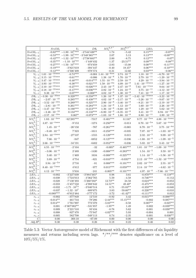
5.5. RESULTS OF THE VAR MODEL FOR RICHEMONT 99
SrelMt Vt D$t MIA,V ∗t MIB,V ∗
t LR3 t rt
SrelMt−1 –0.62*** −1.80 · 107*** –2’544’426** 1.74 –5.42 0.15*** –0.07**SrelMt−2 –0.53*** −1.99 · 107*** –3’548’365*** 2.07 5.13 0.13*** –0.09***SrelMt−3 –0.42*** −1.32 · 107*** –2’738’683** 2.00 –8.75 0.12*** –0.07*SrelMt−4 –0.35*** −1.10 · 107** –1’449’432 –1.37 –23.51** 0.09*** –0.08**SrelMt−5 –0.27*** −1.50 · 107*** –974’659 –2.83 –15.08 0.08*** –0.11***SrelMt−6 –0.19*** –3’821’619 –394’447 –0.40 18.45* 0.06*** –0.10***SrelMt−7 –0.12*** –4’506’499 –978’574 –0.31 12.60 0.03*** –0.06**
Vt−1 1.61 · 10−10*** –0.74*** –0.004 1.44 · 10−8** 2.74 · 10−8 1.18 · 10−11 −6.70 · 10−11
Vt−2 3.15 · 10−10*** –0.61*** –0.006 1.38 · 10−8 1.70 · 10−8 2.79 · 10−11 −1.29 · 10−10
Vt−3 3.47 · 10−10*** –0.48*** –0.014*** 1.55 · 10−8* 2.59 · 10−8 4.29 · 10−11 −3.94 · 10−11
Vt−4 3.93 · 10−10*** –0.38*** –0.021*** 1.58 · 10−8* 4.09 · 10−8 1.41 · 10−10*** −1.27 · 10−10
Vt−5 2.10 · 10−10*** –0.27*** –0.026*** 2.43 · 10−9 2.47 · 10−8 7.61 · 10−11** 9.64 · 10−11
Vt−6 2.18 · 10−10*** –0.17*** –0.036*** 2.82 · 10−9 1.24 · 10−8 3.75 · 10−11 −4.12 · 10−12
Vt−7 9.38 · 10−11* –0.07*** –0.008** 4.02 · 10−9 1.30 · 10−8 7.41 · 10−12 1.17 · 10−11
D$t−1 −3.30 · 10−10** 0.329*** –0.558*** 1.26 · 10−8 1.37 · 10−7 −2.42 · 10−10*** −3.22 · 10−10
D$t−2 −2.07 · 10−10 0.285*** –0.438*** 4.02 · 10−8 −2.17 · 10−8 −5.26 · 10−11 −9.67 · 10−11
D$t−3 −3.52 · 10−10* 0.289*** –0.325*** 2.90 · 10−8 −3.46 · 10−9 −8.21 · 10−11 −2.19 · 10−10
D$t−4 −2.81 · 10−10 0.261*** –0.284*** 1.24 · 10−8 1.12 · 10−7 1.60 · 10−11 2.26 · 10−10
D$t−5 −3.47 · 10−10* 0.190*** –0.213*** 1.36 · 10−8 −6.68 · 10−8 1.29 · 10−12 5.62 · 10−10
D$t−6 −2.46 · 10−10 0.134*** –0.132*** −6.80 · 10−9 −6.35 · 10−8 3.41 · 10−11 6.94 · 10−10*D$t−7 −2.57 · 10−10* 0.067* –0.073*** −1.03 · 10−8 1.66 · 10−8 8.80 · 10−11 4.89 · 10−10
MIA,V ∗t−1 1.83 · 10−4** –62’285*** –7317 –0.401*** 0.116* 9.77 · 10−5** 4.88 · 10−4***
MIA,V ∗t−2 4.87 · 10−4*** –9’153 –1274 –0.250*** –0.014 8.70 · 10−5* 5.67 · 10−4***
MIA,V ∗t−3 1.45 · 10−4 –26’150 –767 –0.261*** –0.065 6.70 · 10−5 3.75 · 10−4*
MIA,V ∗t−4 −9.48 · 10−5 7’323 –1611 –0.258*** –0.035 7.07 · 10−6 −1.03 · 10−4
MIA,V ∗t−5 2.84 · 10−4*** –27’537 –1555 –0.129*** 0.015 2.32 · 10−5 9.09 · 10−5
MIA,V ∗t−6 7.66 · 10−5 –847 –6852 –0.127*** –0.036 −1.68 · 10−6 −1.09 · 10−5
MIA,V ∗t−7 2.66 · 10−4*** –34’191 –6482 –0.052*** –0.036 5.02 · 10−5 3.43 · 10−4*
MIB,V ∗t−1 4.55 · 10−5** –2’104 –32 –0.005* –0.465*** 1.81 · 10−5** −1.09 · 10−4***
MIB,V ∗t−2 −3.06 · 10−6 2’489 –1430 –0.008*** –0.283*** 1.54 · 10−5 3.59 · 10−5
MIB,V ∗t−3 3.40 · 10−5 1’469 1634 –0.008*** –0.225*** 1.14 · 10−5 −5.56 · 10−6
MIB,V ∗t−4 3.89 · 10−6 4’754 –821 –0.010*** –0.035** 2.12 · 10−5** −1.32 · 10−4***
MIB,V ∗t−5 3.94 · 10−5* 2’716 –81 0.008*** –0.101*** 2.02 · 10−5** 2.55 · 10−5
MIB,V ∗t−6 8.40 · 10−5*** 4’812 –977 0.015*** –0.059*** 2.14 · 10−5** −4.62 · 10−5
MIB,V ∗t−7 4.12 · 10−5** 5’916 –241 –0.005** –0.101*** 4.97 · 10−6 −7.66 · 10−5**
LR3 t−1 –0.002 –3’227’039 –3’884’565* 0.98 3.61 –0.870*** –0.118**LR3 t−2 –0.038 1’724’013 –3’362’765 5.59 –4.58 –0.746*** –0.112LR3 t−3 –0.028 –7’130’493 –5’260’592* 12.73** 24.58 –0.624*** –0.053LR3 t−4 –0.033 –5’457’532 –4’988’842 14.51** 49.40* –0.475*** –0.053LR3 t−5 –0.032 −1.71 · 107* –3’040’514 8.71 –55.83** –0.359*** –0.048LR3 t−6 –0.037 −1.32 · 107 –889’675 3.83 –59.60** –0.220*** –0.010LR3 t−7 –0.089*** –6’912’484 –3’77’172 –3.72 –41.42** –0.111*** 0.012
rt−1 –0.002 –377’849 12’510 –0.92 3.42 –0.015*** –0.088***rt−2 –0.014** –461’744 –78’286 –2.44*** 15.15*** –0.002 –0.087***rt−3 0.014** 1’761’997 773’379 –3.83*** –0.58 0.007** –0.027**rt−4 0.001 –3’367’082** –531’857 –1.95** 1.49 0.002 –0.039***rt−5 0.009 2’221’510 93’434 –0.78 5.62 0.001 –0.030***rt−6 0.008 –927’470 –75’947 –4.02*** 5.93 –0.004 0.001rt−7 0.005 582’708 –349’113 0.74 –2.35 0.001 0.030**
C 0.00 369.10 –67.09 0.00 0.00 0.00 0.00Adj.R2 0.30 0.38 0.26 0.18 0.22 0.46 0.02
Table 5.3: Vector Autoregressive model of Richemont with the first differences of six liquiditymeasures and returns including seven lags. */**/*** denotes significance on a level of10%/5%/1%.
100 CHAPTER 5. THE LEAD-LAG BEHAVIOR
A lower liquidity in the tightness dimension leads to lower turnover for the Richemont
stock. The effect is significant for lags one to five. As for Adecco and Baer, a high lagged
dollar depth leads to higher turnover. This time there is significance for all lags. A declining
market impact on the ask-side leads to a lower turnover in the next five minute time space.
There is no interrelation between market impact on the bid-side and turnover. This result
holds for the Richemont stock also in the other direction. Similar to the previous stocks,
there is almost no impact of the lagged liquidity ratio 3 on turnover. The impact of return
on turnover is only significant for lag four; it is negative.
The lagged relative spread has a negative impact on dollar depth which is significant
for lags one to three. Also, rising turnover leads to smaller depth but only for lags larger
than two. There is no influence of the market impact measures on dollar depth and, vice
versa, dollar depth does not influence the market impact measures. Declining liquidity as
measured by the liquidity ratio 3 leads to declining depth with slight significance for lags
one and three. The lagged returns have no influence on dollar depth.
Market impact on the ask-side is not influenced by the lagged relative spread. Rising
turnover leads to lower liquidity on the ask-side with significance for lags one, three and four.
All the lags of market impact on the bid-side have a significant influence on market impact
on the ask-side, but with different signs: The effect is negative for lags one to four and seven
and positive for lags five and six. A rising liquidity ratio 3 leads to declining liquidity as
measured by the market impact on the ask-side on lags two and three. As for the Adecco
and the Baer stocks, rising stock prices tend to be followed by smaller market impact on the
ask-side with significance for lags two, three, four and six.
A rising relative spread leads to a declining market impact on the bid-side on lag four
and a rising one on lag six. Market impact on the ask-side shows only a slight impact on
market impact on the bid-side on lag one. The lagged liquidity ratio 3 induces lower market
impacts on the bid-side on the lags five to seven while the impact of lag four is slightly
positive. Rising stock prices lead to lower liquidity on the bid-side since the impact of lag
two for the lagged returns is significantly positive.
Similar to the previous two stocks, all the lags of the relative spread influence the liquidity
ratio 3 positively. Higher turnovers lead to larger price moves per trade as the relation of
lagged turnover to the liquidity ratio 3 on lags four and five suggests. Rising depth leads
to a smaller liquidity ratio 3. The lagged market impact measures suggest a rising liquidity
ratio 3 for lags one and two on the ask-side and for lags one and four to six on the bid-side.
A rising stock price on lag one leads to a lower liquidity ratio 3, but for lag three the effect
is reversed.
Higher spreads lead to lower returns on all lags, similar to Adecco and Baer. Lagged
turnovers do not influence returns at all. Dollar depth has only a slight impact on lag six.
The lagged market impact on the ask-side leads to higher returns on lags one to three and
seven while the lagged market impact on the bid-side is followed by lower returns. Here,
significance shows up for lags one, four and seven. The liquidity ratio 3 on lag one leads to
lower returns. The impact of lagged returns on the return itself is significantly negative for
lags one to five and shows on the other hand positive significance for lag seven.
None of the constants can be distinguished from zero. The adjusted R2 values range from
46% for the liquidity ratio 3 regression to 2% for the return regression.
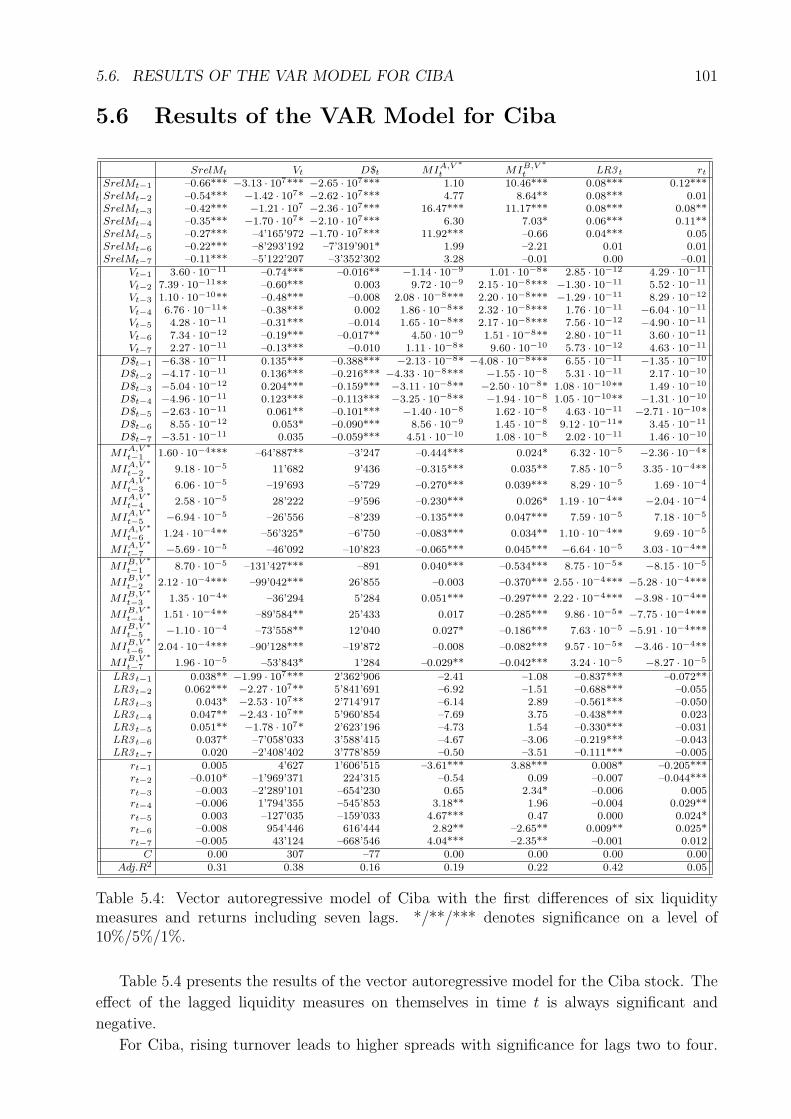
5.6. RESULTS OF THE VAR MODEL FOR CIBA 101
5.6 Results of the VAR Model for Ciba
SrelMt Vt D$t MIA,V ∗t MIB,V ∗
t LR3 t rt
SrelMt−1 –0.66*** −3.13 · 107*** −2.65 · 107*** 1.10 10.46*** 0.08*** 0.12***SrelMt−2 –0.54*** −1.42 · 107* −2.62 · 107*** 4.77 8.64** 0.08*** 0.01SrelMt−3 –0.42*** −1.21 · 107 −2.36 · 107*** 16.47*** 11.17*** 0.08*** 0.08**SrelMt−4 –0.35*** −1.70 · 107* −2.10 · 107*** 6.30 7.03* 0.06*** 0.11**SrelMt−5 –0.27*** –4’165’972 −1.70 · 107*** 11.92*** –0.66 0.04*** 0.05SrelMt−6 –0.22*** –8’293’192 –7’319’901* 1.99 –2.21 0.01 0.01SrelMt−7 –0.11*** –5’122’207 –3’352’302 3.28 –0.01 0.00 –0.01
Vt−1 3.60 · 10−11 –0.74*** –0.016** −1.14 · 10−9 1.01 · 10−8* 2.85 · 10−12 4.29 · 10−11
Vt−2 7.39 · 10−11** –0.60*** 0.003 9.72 · 10−9 2.15 · 10−8*** −1.30 · 10−11 5.52 · 10−11
Vt−3 1.10 · 10−10** –0.48*** –0.008 2.08 · 10−8*** 2.20 · 10−8*** −1.29 · 10−11 8.29 · 10−12
Vt−4 6.76 · 10−11* –0.38*** 0.002 1.86 · 10−8** 2.32 · 10−8*** 1.76 · 10−11 −6.04 · 10−11
Vt−5 4.28 · 10−11 –0.31*** –0.014 1.65 · 10−8** 2.17 · 10−8*** 7.56 · 10−12 −4.90 · 10−11
Vt−6 7.34 · 10−12 –0.19*** –0.017** 4.50 · 10−9 1.51 · 10−8** 2.80 · 10−11 3.60 · 10−11
Vt−7 2.27 · 10−11 –0.13*** –0.010 1.11 · 10−8* 9.60 · 10−10 5.73 · 10−12 4.63 · 10−11
D$t−1 −6.38 · 10−11 0.135*** –0.388*** −2.13 · 10−8* −4.08 · 10−8*** 6.55 · 10−11 −1.35 · 10−10
D$t−2 −4.17 · 10−11 0.136*** –0.216*** −4.33 · 10−8*** −1.55 · 10−8 5.31 · 10−11 2.17 · 10−10
D$t−3 −5.04 · 10−12 0.204*** –0.159*** −3.11 · 10−8** −2.50 · 10−8* 1.08 · 10−10** 1.49 · 10−10
D$t−4 −4.96 · 10−11 0.123*** –0.113*** −3.25 · 10−8** −1.94 · 10−8 1.05 · 10−10** −1.31 · 10−10
D$t−5 −2.63 · 10−11 0.061** –0.101*** −1.40 · 10−8 1.62 · 10−8 4.63 · 10−11 −2.71 · 10−10*D$t−6 8.55 · 10−12 0.053* –0.090*** 8.56 · 10−9 1.45 · 10−8 9.12 · 10−11* 3.45 · 10−11
D$t−7 −3.51 · 10−11 0.035 –0.059*** 4.51 · 10−10 1.08 · 10−8 2.02 · 10−11 1.46 · 10−10
MIA,V ∗t−1 1.60 · 10−4*** –64’887** –3’247 –0.444*** 0.024* 6.32 · 10−5 −2.36 · 10−4*
MIA,V ∗t−2 9.18 · 10−5 11’682 9’436 –0.315*** 0.035** 7.85 · 10−5 3.35 · 10−4**
MIA,V ∗t−3 6.06 · 10−5 –19’693 –5’729 –0.270*** 0.039*** 8.29 · 10−5 1.69 · 10−4
MIA,V ∗t−4 2.58 · 10−5 28’222 –9’596 –0.230*** 0.026* 1.19 · 10−4** −2.04 · 10−4
MIA,V ∗t−5 −6.94 · 10−5 –26’556 –8’239 –0.135*** 0.047*** 7.59 · 10−5 7.18 · 10−5
MIA,V ∗t−6 1.24 · 10−4** –56’325* –6’750 –0.083*** 0.034** 1.10 · 10−4** 9.69 · 10−5
MIA,V ∗t−7 −5.69 · 10−5 –46’092 –10’823 –0.065*** 0.045*** −6.64 · 10−5 3.03 · 10−4**
MIB,V ∗t−1 8.70 · 10−5 –131’427*** –891 0.040*** –0.534*** 8.75 · 10−5* −8.15 · 10−5
MIB,V ∗t−2 2.12 · 10−4*** –99’042*** 26’855 –0.003 –0.370*** 2.55 · 10−4*** −5.28 · 10−4***
MIB,V ∗t−3 1.35 · 10−4* –36’294 5’284 0.051*** –0.297*** 2.22 · 10−4*** −3.98 · 10−4**
MIB,V ∗t−4 1.51 · 10−4** –89’584** 25’433 0.017 –0.285*** 9.86 · 10−5* −7.75 · 10−4***
MIB,V ∗t−5 −1.10 · 10−4 –73’558** 12’040 0.027* –0.186*** 7.63 · 10−5 −5.91 · 10−4***
MIB,V ∗t−6 2.04 · 10−4*** –90’128*** –19’872 –0.008 –0.082*** 9.57 · 10−5* −3.46 · 10−4**
MIB,V ∗t−7 1.96 · 10−5 –53’843* 1’284 –0.029** –0.042*** 3.24 · 10−5 −8.27 · 10−5
LR3 t−1 0.038** −1.99 · 107*** 2’362’906 –2.41 –1.08 –0.837*** –0.072**LR3 t−2 0.062*** −2.27 · 107** 5’841’691 –6.92 –1.51 –0.688*** –0.055LR3 t−3 0.043* −2.53 · 107** 2’714’917 –6.14 2.89 –0.561*** –0.050LR3 t−4 0.047** −2.43 · 107** 5’960’854 –7.69 3.75 –0.438*** 0.023LR3 t−5 0.051** −1.78 · 107* 2’623’196 –4.73 1.54 –0.330*** –0.031LR3 t−6 0.037* –7’058’033 3’588’415 –4.67 –3.06 –0.219*** –0.043LR3 t−7 0.020 –2’408’402 3’778’859 –0.50 –3.51 –0.111*** –0.005
rt−1 0.005 4’627 1’606’515 –3.61*** 3.88*** 0.008* –0.205***rt−2 –0.010* –1’969’371 224’315 –0.54 0.09 –0.007 –0.044***rt−3 –0.003 –2’289’101 –654’230 0.65 2.34* –0.006 0.005rt−4 –0.006 1’794’355 –545’853 3.18** 1.96 –0.004 0.029**rt−5 0.003 –127’035 –159’033 4.67*** 0.47 0.000 0.024*rt−6 –0.008 954’446 616’444 2.82** –2.65** 0.009** 0.025*rt−7 –0.005 43’124 –668’546 4.04*** –2.35** –0.001 0.012
C 0.00 307 –77 0.00 0.00 0.00 0.00Adj.R2 0.31 0.38 0.16 0.19 0.22 0.42 0.05
Table 5.4: Vector autoregressive model of Ciba with the first differences of six liquiditymeasures and returns including seven lags. */**/*** denotes significance on a level of10%/5%/1%.
Table 5.4 presents the results of the vector autoregressive model for the Ciba stock. The
effect of the lagged liquidity measures on themselves in time t is always significant and
negative.
For Ciba, rising turnover leads to higher spreads with significance for lags two to four.
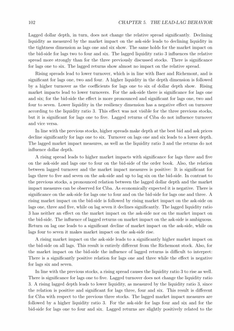
102 CHAPTER 5. THE LEAD-LAG BEHAVIOR
Lagged dollar depth, in turn, does not change the relative spread significantly. Declining
liquidity as measured by the market impact on the ask-side leads to declining liquidity in
the tightness dimension as lags one and six show. The same holds for the market impact on
the bid-side for lags two to four and six. The lagged liquidity ratio 3 influences the relative
spread more strongly than for the three previously discussed stocks. There is significance
for lags one to six. The lagged returns show almost no impact on the relative spread.
Rising spreads lead to lower turnover, which is in line with Baer and Richemont, and is
significant for lags one, two and four. A higher liquidity in the depth dimension is followed
by a higher turnover as the coefficients for lags one to six of dollar depth show. Rising
market impacts lead to lower turnovers. For the ask-side there is significance for lags one
and six; for the bid-side the effect is more pronounced and significant for lags one, two and
four to seven. Lower liquidity in the resiliency dimension has a negative effect on turnover
according to the liquidity ratio 3. This effect was not visible for the three previous stocks,
but it is significant for lags one to five. Lagged returns of Ciba do not influence turnover
and vice versa.
In line with the previous stocks, higher spreads make depth at the best bid and ask prices
decline significantly for lags one to six. Turnover on lags one and six leads to a lower depth.
The lagged market impact measures, as well as the liquidity ratio 3 and the returns do not
influence dollar depth.
A rising spread leads to higher market impacts with significance for lags three and five
on the ask-side and lags one to four on the bid-side of the order book. Also, the relation
between lagged turnover and the market impact measures is positive: It is significant for
lags three to five and seven on the ask-side and up to lag six on the bid-side. In contrast to
the previous stocks, a pronounced relation between the lagged dollar depth and the market
impact measures can be observed for Ciba. As economically expected it is negative. There is
significance on the ask-side for lags one to four and on the bid-side for lags one and three. A
rising market impact on the bid-side is followed by rising market impact on the ask-side on
lags one, three and five, while on lag seven it declines significantly. The lagged liquidity ratio
3 has neither an effect on the market impact on the ask-side nor on the market impact on
the bid-side. The influence of lagged returns on market impact on the ask-side is ambiguous.
Return on lag one leads to a significant decline of market impact on the ask-side, while on
lags four to seven it makes market impact on the ask-side rise.
A rising market impact on the ask-side leads to a significantly higher market impact on
the bid-side on all lags. This result is entirely different from the Richemont stock. Also, for
the market impact on the bid-side the influence of lagged returns is difficult to interpret:
There is a significantly positive relation for lags one and three while the effect is negative
for lags six and seven.
In line with the previous stocks, a rising spread causes the liquidity ratio 3 to rise as well.
There is significance for lags one to five. Lagged turnover does not change the liquidity ratio
3. A rising lagged depth leads to lower liquidity, as measured by the liquidity ratio 3, since
the relation is positive and significant for lags three, four and six. This result is different
for Ciba with respect to the previous three stocks. The lagged market impact measures are
followed by a higher liquidity ratio 3. For the ask-side for lags four and six and for the
bid-side for lags one to four and six. Lagged returns are slightly positively related to the
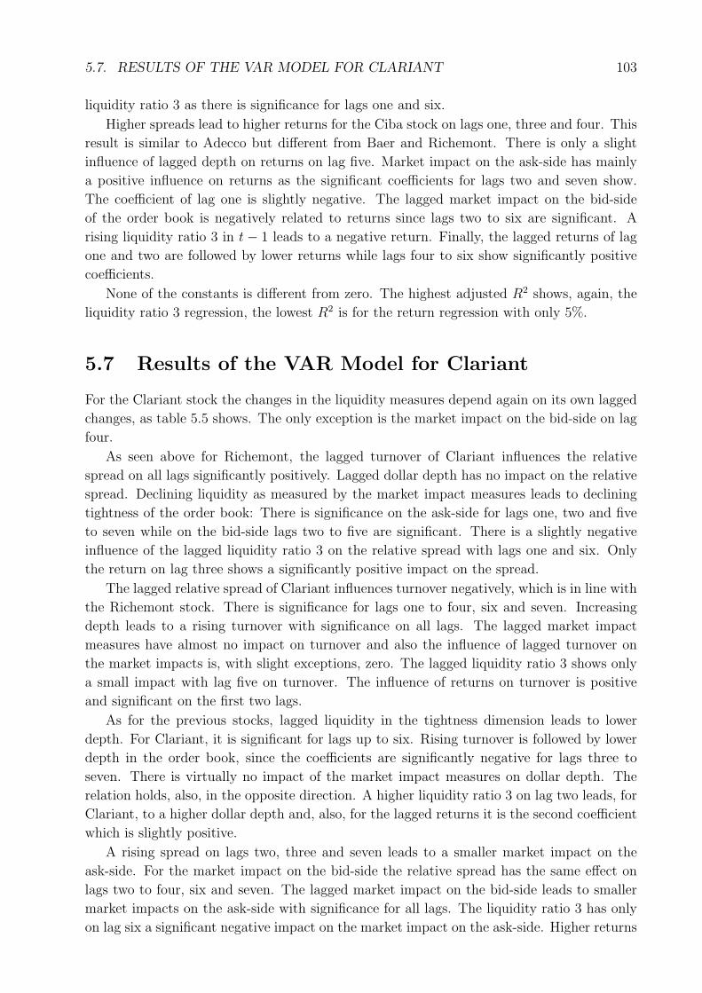
5.7. RESULTS OF THE VAR MODEL FOR CLARIANT 103
liquidity ratio 3 as there is significance for lags one and six.
Higher spreads lead to higher returns for the Ciba stock on lags one, three and four. This
result is similar to Adecco but different from Baer and Richemont. There is only a slight
influence of lagged depth on returns on lag five. Market impact on the ask-side has mainly
a positive influence on returns as the significant coefficients for lags two and seven show.
The coefficient of lag one is slightly negative. The lagged market impact on the bid-side
of the order book is negatively related to returns since lags two to six are significant. A
rising liquidity ratio 3 in t− 1 leads to a negative return. Finally, the lagged returns of lag
one and two are followed by lower returns while lags four to six show significantly positive
coefficients.
None of the constants is different from zero. The highest adjusted R2 shows, again, the
liquidity ratio 3 regression, the lowest R2 is for the return regression with only 5%.
5.7 Results of the VAR Model for Clariant
For the Clariant stock the changes in the liquidity measures depend again on its own lagged
changes, as table 5.5 shows. The only exception is the market impact on the bid-side on lag
four.
As seen above for Richemont, the lagged turnover of Clariant influences the relative
spread on all lags significantly positively. Lagged dollar depth has no impact on the relative
spread. Declining liquidity as measured by the market impact measures leads to declining
tightness of the order book: There is significance on the ask-side for lags one, two and five
to seven while on the bid-side lags two to five are significant. There is a slightly negative
influence of the lagged liquidity ratio 3 on the relative spread with lags one and six. Only
the return on lag three shows a significantly positive impact on the spread.
The lagged relative spread of Clariant influences turnover negatively, which is in line with
the Richemont stock. There is significance for lags one to four, six and seven. Increasing
depth leads to a rising turnover with significance on all lags. The lagged market impact
measures have almost no impact on turnover and also the influence of lagged turnover on
the market impacts is, with slight exceptions, zero. The lagged liquidity ratio 3 shows only
a small impact with lag five on turnover. The influence of returns on turnover is positive
and significant on the first two lags.
As for the previous stocks, lagged liquidity in the tightness dimension leads to lower
depth. For Clariant, it is significant for lags up to six. Rising turnover is followed by lower
depth in the order book, since the coefficients are significantly negative for lags three to
seven. There is virtually no impact of the market impact measures on dollar depth. The
relation holds, also, in the opposite direction. A higher liquidity ratio 3 on lag two leads, for
Clariant, to a higher dollar depth and, also, for the lagged returns it is the second coefficient
which is slightly positive.
A rising spread on lags two, three and seven leads to a smaller market impact on the
ask-side. For the market impact on the bid-side the relative spread has the same effect on
lags two to four, six and seven. The lagged market impact on the bid-side leads to smaller
market impacts on the ask-side with significance for all lags. The liquidity ratio 3 has only
on lag six a significant negative impact on the market impact on the ask-side. Higher returns
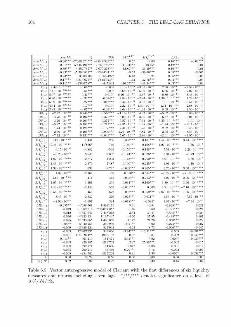
104 CHAPTER 5. THE LEAD-LAG BEHAVIOR
SrelMt Vt D$t MIA,V ∗t MIB,V ∗
t LR3 t rt
SrelMt−1 –0.66*** –7’069’374*** –2’012’339*** 0.57 2.00 0.10*** –0.08***SrelMt−2 –0.51*** –5’445’191*** –2’760’742*** –11.94*** –18.45* 0.12*** –0.01SrelMt−3 –0.39*** –4’552’762** –2’070’278*** –12.89*** –31.49*** 0.10*** –0.01SrelMt−4 –0.33*** –5’394’821** –1’834’441** –5.63 –39.66*** 0.08*** –0.06*SrelMt−5 –0.23*** –3’003’786 –1’358’422* –6.43 –15.27 0.06*** –0.05SrelMt−6 –0.17*** –4’816’675** –1’645’523** –1.42 –32.76*** 0.04*** 0.05SrelMt−7 –0.11*** –2’960’587* –447’833 –16.67*** –41.44*** 0.03*** 0.04
Vt−1 2.44 · 10−10** –0.66*** –0.005 8.13 · 10−9 −3.05 · 10−8 2.38 · 10−11 −2.54 · 10−10
Vt−2 7.41 · 10−10*** –0.51*** –0.007 3.68 · 10−8 −6.50 · 10−8 6.36 · 10−11 −2.07 · 10−10
Vt−3 5.97 · 10−10*** –0.42*** –0.010* 6.16 · 10−8* −3.37 · 10−8 6.89 · 10−11 3.43 · 10−10
Vt−4 6.20 · 10−10*** –0.32*** –0.014** 4.54 · 10−8 −2.84 · 10−9 1.36 · 10−10** 1.24 · 10−10
Vt−5 5.09 · 10−10*** –0.27*** –0.017*** 3.42 · 10−8 4.07 · 10−8 1.01 · 10−10 −8.51 · 10−12
Vt−6 4.54 · 10−10*** –0.17*** –0.010* 2.22 · 10−8 1.59 · 10−7* 1.11 · 10−10* 2.68 · 10−10
Vt−7 2.82 · 10−10*** –0.07*** –0.011** 3.68 · 10−8 −1.22 · 10−8 8.69 · 10−11 2.50 · 10−10
D$t−1 −2.22 · 10−10 0.240*** –0.510*** −1.16 · 10−8 4.87 · 10−8 −5.07 · 10−11 6.86 · 10−11
D$t−2 −4.78 · 10−10 0.192*** –0.375*** 8.00 · 10−8 3.56 · 10−8 −6.87 · 10−11 −5.01 · 10−10
D$t−3 −3.29 · 10−10 0.203*** –0.272*** 5.57 · 10−8 7.64 · 10−8 −3.35 · 10−10** −1.01 · 10−9
D$t−4 −5.27 · 10−10 0.152*** –0.219*** −2.95 · 10−8 1.48 · 10−7 −1.24 · 10−10 −3.11 · 10−10
D$t−5 −1.74 · 10−10 0.120*** –0.168*** 2.41 · 10−8 −1.28 · 10−7 −2.02 · 10−10 −6.48 · 10−10
D$t−6 −2.56 · 10−10 0.106*** –0.099*** −4.20 · 10−10 7.82 · 10−8 −2.98 · 10−11 −8.55 · 10−10
D$t−7 −7.12 · 10−11 0.133*** –0.041*** 5.65 · 10−8 2.86 · 10−7 −2.01 · 10−10 −1.95 · 10−10
MIA,V ∗t−1 1.12 · 10−4** –7’441 –286 –0.363*** 0.101*** 1.47 · 10−4*** 3.44 · 10−4***
MIA,V ∗t−2 2.45 · 10−4*** –11’866* –749 –0.160*** 0.168*** 1.07 · 10−4*** 7.66 · 10−5
MIA,V ∗t−3 6.15 · 10−6 –4’882 –599 –0.159*** 0.158*** 7.51 · 10−6 2.28 · 10−4**
MIA,V ∗t−4 −6.20 · 10−5 3’843 2’067 –0.174*** 0.326*** 3.91 · 10−5 −1.23 · 10−4
MIA,V ∗t−5 1.82 · 10−4*** –2’877 1’203 –0.113*** 0.260*** 5.07 · 10−5* −4.88 · 10−5
MIA,V ∗t−6 1.43 · 10−4*** 2’370 2’487 –0.100*** 0.225*** 1.01 · 10−5 1.10 · 10−5
MIA,V ∗t−7 1.38 · 10−4*** 336 4’074* –0.042*** 0.205*** 3.75 · 10−5 3.60 · 10−4***
MIB,V ∗t−1 1.89 · 10−5 –2’164 –59 –0.010** –0.584*** −6.72 · 10−6 −7.19 · 10−5**
MIB,V ∗t−2 4.16 · 10−5** 411 442 –0.035*** –0.213*** −1.07 · 10−6 −2.06 · 10−4***
MIB,V ∗t−3 1.05 · 10−4*** 1’401 291 –0.034*** –0.160*** 1.89 · 10−5* −3.00 · 10−4***
MIB,V ∗t−4 7.40 · 10−5*** –2’440 552 –0.045*** 0.003 1.91 · 10−5* −2.16 · 10−4***
MIB,V ∗t−5 8.56 · 10−5*** 450 672 –0.037*** –0.059*** 2.87 · 10−5*** −1.06 · 10−4***
MIB,V ∗t−6 8.45 · 10−6 –2’332 270 –0.025*** –0.031** 1.56 · 10−5 −7.62 · 10−5*
MIB,V ∗t−7 −2.06 · 10−5 –1’997 324 –0.018*** –0.024* 1.87 · 10−6 −7.44 · 10−6
LR3t−1 –0.055** –4’096’761 1’462’171 5.21 –0.94 –0.869*** 0.027LR3t−2 –0.049 –1’562’316 2’970’608** –1.48 16.60 –0.721*** 0.024LR3t−3 –0.012 –4’657’542 2’418’213 –3.34 39.47 –0.565*** –0.024LR3t−4 0.026 –4’323’134 1’165’447 –4.60 37.95 –0.438*** 0.107LR3t−5 –0.025 –7’153’495* 1’400’059 –11.72 21.26 –0.350*** 0.029LR3t−6 –0.058* –5’940’254 340’966 –16.21** –3.02 –0.224*** –0.007LR3t−7 –0.009 –3’380’424 821’043 –4.63 8.73 –0.096*** –0.045
rt−1 –0.003 1’290’733* 349’666 –3.94*** –13.31*** 0.005 –0.091***rt−2 0.001 1’716’914** 499’210* –0.07 –5.81 –0.002 –0.043***rt−3 0.013** –561’119 184’471 –5.62*** –3.92 0.006* –0.030***rt−4 –0.003 820’155 –219’762 2.27 25.98*** –0.002 –0.015rt−5 0.008 –692’771 114’680 –2.84* 4.03 –0.001 0.014rt−6 0.005 200’210 47’446 –6.29*** 3.76 –0.002 –0.009rt−7 –0.005 –954’783 –215’263 0.81 1.36 –0.005* 0.038***
C 0.00 38.22 8.56 0.00 0.00 0.00 0.00Adj.R2 0.32 0.32 0.22 0.15 0.30 0.44 0.02
Table 5.5: Vector autoregressive model of Clariant with the first differences of six liquiditymeasures and returns including seven lags. */**/*** denotes significance on a level of10%/5%/1%.
5.8. RESULTS OF THE VAR MODEL FOR GIVAUDAN 105
are followed by smaller market impacts on the ask-side with significance for lags one, three,
five and six.
The market impact on the bid-side is significantly positively influenced by the lagged
market impact on the ask-side for all lags, while the liquidity ratio 3 has no influence at
all. Rising returns in lag one are followed by declining market impacts on the bid-side. In
contrast to this, the returns of lag four lead to higher market impacts on the bid-side.
Higher relative spreads lead to higher liquidity ratios 3 with significance for all lags.
Lagged turnover has only little influence on the liquidity ratio 3 for the Clariant stock on
lags four and six. This in contrast to Baer, for example. Higher dollar depth on lag three
is followed by a smaller liquidity ratio 3. The significant lagged values of the market impact
measures on the ask- and on the bid-side lead to rising liquidity ratios 3. There is significance
on the ask-side for lags one, two and five while on the bid-side lags three to five are significant.
There is only a slight impact of returns at lags three and seven on the liquidity ratio 3.
The lagged relative spread has a significantly negative impact on returns with lags one
and four. Lagged turnover and lagged depth do not influence returns. The market impact
on the ask-side leads to higher returns on lags one, three and seven. The market impact on
the bid-side is followed by lower returns. There is significance for lags one to six. The lagged
liquidity ratio 3 does not influence returns. Finally, rising returns on lags one to three lead
to smaller returns in time t while on lag seven the effect is reversed.
The constants of the vector autoregressions are all zero and the adjusted R2 is again
highest for the liquidity ratio 3 regression and lowest for the returns regression.
5.8 Results of the VAR Model for Givaudan
The results of the vector autoregressive model for Givaudan are presented in table 5.6. As for
the previous stocks, Givaudan shows significantly negative impacts of the liquidity measures’
own lags on the respective liquidity measures in time t.
Rising turnover on lags two and three leads to a rising relative spread. Dollar depth has
for the Givaudan stock no influence on the spread. All the significant values of the market
impact measures are followed by rising relative spreads. For the market impact on the ask-
side there is significance for all lags, for the market impact on the bid-side lags one to four
are significant. The lagged liquidity ratio 3 has only a slight impact on the relative spread
on lags six and seven. The return on lag three has a negative effect on the spread.
A rising spread leads to a declining turnover. Lags one to four and six show a signifi-
cantly negative relation of lagged relative spread to turnover. Also, rising depth leads to a
rising turnover for lags one and two. Declining liquidity as measured by the market impact
measures leads, in general, to a declining turnover. On the ask-side there is significance for
lags one to six and on the bid-side for lags one and two. Only the market impact on the
bid-side shows a slightly negative impact on returns. The lagged liquidity ratio 3 has no
impact at all on turnover. A higher return in time t − 1 leads to a higher turnover in time
t. On the other hand, on lags four, five and seven this interrelation is reversed.
There is no significant impact of lagged relative spread on dollar depth. Neither does
lagged turnover influence dollar depth. Market impact on the ask-side shows some positive
significance on lag seven for an impact on dollar depth, while the market impact on the bid-
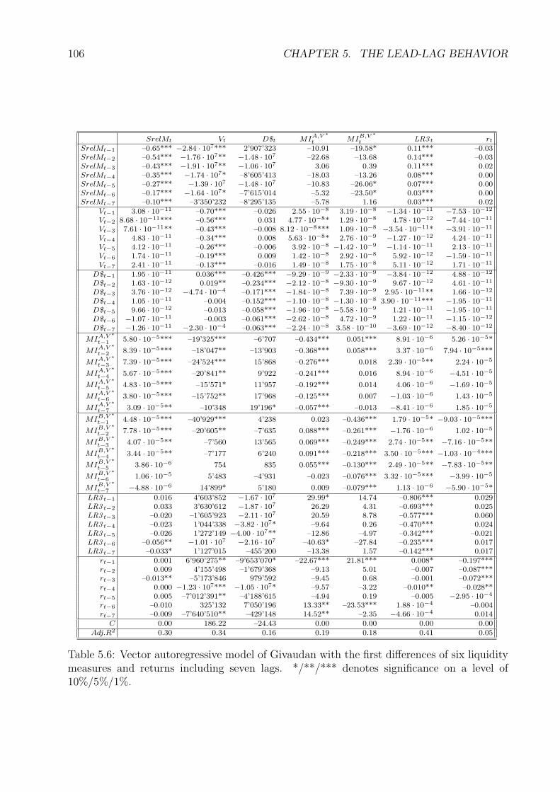
106 CHAPTER 5. THE LEAD-LAG BEHAVIOR
SrelMt Vt D$t MIA,V ∗t MIB,V ∗
t LR3 t rt
SrelMt−1 –0.65*** −2.84 · 107*** 2’907’323 –10.91 –19.58* 0.11*** –0.03SrelMt−2 –0.54*** −1.76 · 107** −1.48 · 107 –22.68 –13.68 0.14*** –0.03SrelMt−3 –0.43*** −1.91 · 107** −1.06 · 107 3.06 0.39 0.11*** 0.02SrelMt−4 –0.35*** −1.74 · 107* –8’605’413 –18.03 –13.26 0.08*** 0.00SrelMt−5 –0.27*** −1.39 · 107 −1.48 · 107 –10.83 –26.06* 0.07*** 0.00SrelMt−6 –0.17*** −1.64 · 107* –7’615’014 –5.32 –23.50* 0.03*** 0.00SrelMt−7 –0.10*** –3’350’232 –8’295’135 –5.78 1.16 0.03*** 0.02
Vt−1 3.08 · 10−11 –0.70*** –0.026 2.55 · 10−8 3.19 · 10−8 −1.34 · 10−11 −7.53 · 10−12
Vt−2 8.68 · 10−11*** –0.56*** 0.031 4.77 · 10−8* 1.29 · 10−8 4.78 · 10−12 −7.44 · 10−11
Vt−3 7.61 · 10−11** –0.43*** –0.008 8.12 · 10−8*** 1.09 · 10−8 −3.54 · 10−11* −3.91 · 10−11
Vt−4 4.83 · 10−11 –0.34*** 0.008 5.63 · 10−8* 2.76 · 10−9 −1.27 · 10−12 4.24 · 10−11
Vt−5 4.12 · 10−11 –0.26*** –0.006 3.92 · 10−8 −1.42 · 10−9 −1.14 · 10−11 2.13 · 10−11
Vt−6 1.74 · 10−11 –0.19*** 0.009 1.42 · 10−8 2.92 · 10−8 5.92 · 10−12 −1.59 · 10−11
Vt−7 2.41 · 10−11 –0.13*** –0.016 1.49 · 10−8 1.75 · 10−8 5.11 · 10−12 1.71 · 10−11
D$t−1 1.95 · 10−11 0.036*** –0.426*** −9.29 · 10−9 −2.33 · 10−9 −3.84 · 10−12 4.88 · 10−12
D$t−2 1.63 · 10−12 0.019** –0.234*** −2.12 · 10−8 −9.30 · 10−9 9.67 · 10−12 4.61 · 10−11
D$t−3 3.76 · 10−12 −4.74 · 10−4 –0.171*** −1.84 · 10−8 7.39 · 10−9 2.95 · 10−11** 1.66 · 10−12
D$t−4 1.05 · 10−11 –0.004 –0.152*** −1.10 · 10−8 −1.30 · 10−8 3.90 · 10−11*** −1.95 · 10−11
D$t−5 9.66 · 10−12 –0.013 –0.058*** −1.96 · 10−8 −5.58 · 10−9 1.21 · 10−11 −1.95 · 10−11
D$t−6 −1.07 · 10−11 –0.003 –0.061*** −2.62 · 10−8 4.72 · 10−9 1.22 · 10−11 −1.15 · 10−12
D$t−7 −1.26 · 10−11 −2.30 · 10−4 –0.063*** −2.24 · 10−8 3.58 · 10−10 −3.69 · 10−12 −8.40 · 10−12
MIA,V ∗t−1 5.80 · 10−5*** –19’325*** –6’707 –0.434*** 0.051*** 8.91 · 10−6 5.26 · 10−5*
MIA,V ∗t−2 8.39 · 10−5*** –18’047** –13’903 –0.368*** 0.058*** 3.37 · 10−6 7.94 · 10−5***
MIA,V ∗t−3 7.39 · 10−5*** –24’524*** 15’868 –0.276*** 0.018 2.39 · 10−5** 2.24 · 10−5
MIA,V ∗t−4 5.67 · 10−5*** –20’841** 9’922 –0.241*** 0.016 8.94 · 10−6 −4.51 · 10−5
MIA,V ∗t−5 4.83 · 10−5*** –15’571* 11’957 –0.192*** 0.014 4.06 · 10−6 −1.69 · 10−5
MIA,V ∗t−6 3.80 · 10−5*** –15’752** 17’968 –0.125*** 0.007 −1.03 · 10−6 1.43 · 10−5
MIA,V ∗t−7 3.09 · 10−5** –10’348 19’196* –0.057*** –0.013 −8.41 · 10−6 1.85 · 10−5
MIB,V ∗t−1 4.48 · 10−5*** –40’929*** 4’238 0.023 –0.436*** 1.79 · 10−5* −9.03 · 10−5***
MIB,V ∗t−2 7.78 · 10−5*** –20’605** –7’635 0.088*** –0.261*** −1.76 · 10−6 1.02 · 10−5
MIB,V ∗t−3 4.07 · 10−5** –7’560 13’565 0.069*** –0.249*** 2.74 · 10−5** −7.16 · 10−5**
MIB,V ∗t−4 3.44 · 10−5** –7’177 6’240 0.091*** –0.218*** 3.50 · 10−5*** −1.03 · 10−4***
MIB,V ∗t−5 3.86 · 10−6 754 835 0.055*** –0.130*** 2.49 · 10−5** −7.83 · 10−5**
MIB,V ∗t−6 1.06 · 10−5 5’483 –4’931 –0.023 –0.076*** 3.32 · 10−5*** −3.99 · 10−5
MIB,V ∗t−7 −4.88 · 10−6 14’899* 5’180 0.009 –0.079*** 1.13 · 10−6 −5.90 · 10−5*
LR3 t−1 0.016 4’603’852 −1.67 · 107 29.99* 14.74 –0.806*** 0.029LR3 t−2 0.033 3’630’612 −1.87 · 107 26.29 4.31 –0.693*** 0.025LR3 t−3 –0.020 –1’605’923 −2.11 · 107 20.59 8.78 –0.577*** 0.060LR3 t−4 –0.023 1’044’338 −3.82 · 107* –9.64 0.26 –0.470*** 0.024LR3 t−5 –0.026 1’272’149 −4.00 · 107** –12.86 –4.97 –0.342*** –0.021LR3 t−6 –0.056** −1.01 · 107 −2.16 · 107 –40.63* –27.84 –0.235*** 0.017LR3 t−7 –0.033* 1’127’015 –455’200 –13.38 1.57 –0.142*** 0.017
rt−1 0.001 6’960’275** –9’653’070* –22.67*** 21.81*** 0.008* –0.197***rt−2 0.009 4’155’498 –1’679’368 –9.13 5.01 –0.007 –0.087***rt−3 –0.013** –5’173’846 979’592 –9.45 0.68 –0.001 –0.072***rt−4 0.000 −1.23 · 107*** −1.05 · 107* –9.57 –3.22 –0.010** –0.028**rt−5 0.005 –7’012’391** –4’188’615 –4.94 0.19 –0.005 −2.95 · 10−4
rt−6 –0.010 325’132 7’050’196 13.33** –23.53*** 1.88 · 10−4 –0.004rt−7 –0.009 –7’640’510** –429’148 14.52** –2.35 −4.66 · 10−4 0.014
C 0.00 186.22 –24.43 0.00 0.00 0.00 0.00Adj.R2 0.30 0.34 0.16 0.19 0.18 0.41 0.05
Table 5.6: Vector autoregressive model of Givaudan with the first differences of six liquiditymeasures and returns including seven lags. */**/*** denotes significance on a level of10%/5%/1%.
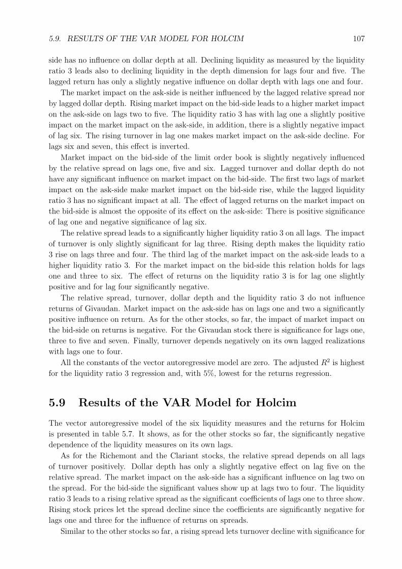
5.9. RESULTS OF THE VAR MODEL FOR HOLCIM 107
side has no influence on dollar depth at all. Declining liquidity as measured by the liquidity
ratio 3 leads also to declining liquidity in the depth dimension for lags four and five. The
lagged return has only a slightly negative influence on dollar depth with lags one and four.
The market impact on the ask-side is neither influenced by the lagged relative spread nor
by lagged dollar depth. Rising market impact on the bid-side leads to a higher market impact
on the ask-side on lags two to five. The liquidity ratio 3 has with lag one a slightly positive
impact on the market impact on the ask-side, in addition, there is a slightly negative impact
of lag six. The rising turnover in lag one makes market impact on the ask-side decline. For
lags six and seven, this effect is inverted.
Market impact on the bid-side of the limit order book is slightly negatively influenced
by the relative spread on lags one, five and six. Lagged turnover and dollar depth do not
have any significant influence on market impact on the bid-side. The first two lags of market
impact on the ask-side make market impact on the bid-side rise, while the lagged liquidity
ratio 3 has no significant impact at all. The effect of lagged returns on the market impact on
the bid-side is almost the opposite of its effect on the ask-side: There is positive significance
of lag one and negative significance of lag six.
The relative spread leads to a significantly higher liquidity ratio 3 on all lags. The impact
of turnover is only slightly significant for lag three. Rising depth makes the liquidity ratio
3 rise on lags three and four. The third lag of the market impact on the ask-side leads to a
higher liquidity ratio 3. For the market impact on the bid-side this relation holds for lags
one and three to six. The effect of returns on the liquidity ratio 3 is for lag one slightly
positive and for lag four significantly negative.
The relative spread, turnover, dollar depth and the liquidity ratio 3 do not influence
returns of Givaudan. Market impact on the ask-side has on lags one and two a significantly
positive influence on return. As for the other stocks, so far, the impact of market impact on
the bid-side on returns is negative. For the Givaudan stock there is significance for lags one,
three to five and seven. Finally, turnover depends negatively on its own lagged realizations
with lags one to four.
All the constants of the vector autoregressive model are zero. The adjusted R2 is highest
for the liquidity ratio 3 regression and, with 5%, lowest for the returns regression.
5.9 Results of the VAR Model for Holcim
The vector autoregressive model of the six liquidity measures and the returns for Holcim
is presented in table 5.7. It shows, as for the other stocks so far, the significantly negative
dependence of the liquidity measures on its own lags.
As for the Richemont and the Clariant stocks, the relative spread depends on all lags
of turnover positively. Dollar depth has only a slightly negative effect on lag five on the
relative spread. The market impact on the ask-side has a significant influence on lag two on
the spread. For the bid-side the significant values show up at lags two to four. The liquidity
ratio 3 leads to a rising relative spread as the significant coefficients of lags one to three show.
Rising stock prices let the spread decline since the coefficients are significantly negative for
lags one and three for the influence of returns on spreads.
Similar to the other stocks so far, a rising spread lets turnover decline with significance for
108 CHAPTER 5. THE LEAD-LAG BEHAVIOR
SrelMt Vt D$t MIA,V ∗t MIB,V ∗
t LR3 t rt
SrelMt−1 –0.71*** −2.64 · 107*** −1.78 · 107*** 1.86 –6.89 0.10*** –0.06**SrelMt−2 –0.59*** −3.17 · 107*** −1.95 · 107*** 28.07*** –5.57 0.12*** –0.10***SrelMt−3 –0.50*** −1.78 · 107* −1.44 · 107*** 23.23* –17.63 0.11*** –0.14***SrelMt−4 –0.41*** −2.39 · 107** –9’991’002** 6.92 –10.78 0.09*** –0.08*SrelMt−5 –0.30*** −1.23 · 107 −1.03 · 107*** –5.94 –22.10* 0.06*** –0.09**SrelMt−6 –0.22*** –5’316’281 –4’480’681 –16.51 –1.12 0.03*** 0.01SrelMt−7 –0.14*** 899’583 –2’172’127 –16.00 8.55 0.02*** –0.03
Vt−1 6.43 · 10−11*** –0.68*** –0.005 1.65 · 10−8 3.10 · 10−8** 3.54 · 10−11*** −3.03 · 10−11
Vt−2 1.01 · 10−10*** –0.57*** 0.005 4.70 · 10−8** 3.70 · 10−8** 3.87 · 10−11** −1.39 · 10−11
Vt−3 8.03 · 10−11*** –0.47*** –0.011 5.07 · 10−8** 3.14 · 10−8 3.22 · 10−11* 1.01 · 10−12
Vt−4 1.01 · 10−10*** –0.31*** –0.006 4.56 · 10−8* 4.30 · 10−8** 2.67 · 10−11 7.35 · 10−12
Vt−5 6.59 · 10−11** –0.25*** –0.009 4.61 · 10−8* 2.28 · 10−8 2.17 · 10−11 3.55 · 10−11
Vt−6 8.52 · 10−11*** –0.17*** –0.003 3.06 · 10−8 2.74 · 10−8 2.69 · 10−11* 4.70 · 10−12
Vt−7 7.15 · 10−11*** –0.09*** –0.006 3.02 · 10−8 3.08 · 10−8** 1.55 · 10−11 2.26 · 10−11
D$t−1 −8.61 · 10−11 0.194*** –0.422*** −5.18 · 10−8 4.65 · 10−8 1.67 · 10−11 1.60 · 10−10
D$t−2 −7.35 · 10−11 0.235*** –0.293*** −1.69 · 10−8 −5.76 · 10−8 1.80 · 10−11 1.29 · 10−10
D$t−3 −9.03 · 10−11 0.146*** –0.245*** −9.34 · 10−9 1.49 · 10−8 −2.21 · 10−11 4.59 · 10−11
D$t−4 −8.91 · 10−11 0.095*** –0.172*** −1.70 · 10−8 −1.05 · 10−8 −5.35 · 10−12 5.02 · 10−11
D$t−5 −1.67 · 10−10** 0.175*** –0.104*** −3.83 · 10−8 −3.22 · 10−8 5.31 · 10−11 1.38 · 10−10
D$t−6 −3.81 · 10−11 0.032 –0.097*** −4.88 · 10−8 −5.87 · 10−8 2.78 · 10−11 −4.95 · 10−11
D$t−7 −9.35 · 10−11 –0.071** –0.044*** −6.07 · 10−8 −5.47 · 10−8 −1.44 · 10−11 1.00 · 10−10
MIA,V ∗t−1 1.15 · 10−5 –25’981*** –6’991* –0.430*** 0.020* 2.69 · 10−5*** 2.86 · 10−6
MIA,V ∗t−2 4.33 · 10−5** –19’154** –3’132 –0.311*** 0.027** 5.45 · 10−5*** 7.85 · 10−5**
MIA,V ∗t−3 1.12 · 10−5 –12’967 –1’991 –0.251*** 0.010 2.34 · 10−5** 1.34 · 10−4***
MIA,V ∗t−4 −6.76 · 10−6 –15’694 –3’094 –0.168*** 0.002 2.03 · 10−5** 6.80 · 10−5*
MIA,V ∗t−5 1.14 · 10−5 –13’884 –370 –0.156*** –0.004 1.79 · 10−5* 1.55 · 10−4***
MIA,V ∗t−6 1.52 · 10−5 –12’157 –4’358 –0.115*** 0.010 2.18 · 10−5** 7.84 · 10−5*
MIA,V ∗t−7 −1.15 · 10−5 –25’184*** 149 –0.054*** –0.006 5.43 · 10−6 8.55 · 10−5*
MIB,V ∗t−1 9.82 · 10−6 –47’544*** 467 0.023 –0.449*** 4.49 · 10−5*** −3.07 · 10−5
MIB,V ∗t−2 8.59 · 10−5*** –28’267** –1’934 0.014 –0.342*** 4.53 · 10−5*** −9.02 · 10−6
MIB,V ∗t−3 7.93 · 10−5*** –27’561** –2’597 0.025 –0.209*** 2.73 · 10−5** −6.97 · 10−5
MIB,V ∗t−4 4.64 · 10−5** –7’423 2’884 –0.002 –0.184*** 2.98 · 10−5** −1.01 · 10−4**
MIB,V ∗t−5 −3.87 · 10−6 12’434 1’635 0.013 –0.157*** 2.24 · 10−5* −2.78 · 10−5
MIB,V ∗t−6 −2.46 · 10−6 –154 2’258 0.014 –0.118*** 1.40 · 10−5 −1.02 · 10−4**
MIB,V ∗t−7 −2.85 · 10−5 –14’435 1’717 –0.011 –0.063*** −1.38 · 10−6 1.77 · 10−6
LR3 t−1 0.088*** 1.62 · 107 2’930’593 4.88 –6.47 –0.857*** –0.012LR3 t−2 0.075*** 1.43 · 107 691’185 –32.27 22.89 –0.716*** 0.014LR3 t−3 0.072** 662’465 –418’773 –14.77 41.14** –0.613*** –0.008LR3 t−4 0.050 991’834 –1’714’004 –0.88 48.08** –0.514*** 0.036LR3 t−5 0.014 5’170’802 –3’329’099 25.75 14.30 –0.365*** 0.026LR3 t−6 0.024 –8’842’102 –4’822’882 33.61 2.35 –0.239*** 0.066LR3 t−7 –0.023 –8’488’475 –4’795’353 –5.41 10.72 –0.134*** –0.015
rt−1 –0.017*** 3’169’054 –2’479’149* –9.86** 24.65*** –0.003 –0.168***rt−2 –0.009 –2’132’963 –142’965 –10.80** 10.07** –0.002 –0.067***rt−3 –0.015** 1’489’101 911’206 –18.44*** 16.24*** 0.001 –0.042***rt−4 –0.009 5’607’410* –430’241 –3.47 –2.35 0.001 –0.041***rt−5 0.002 –551’572 382’552 –2.86 12.05*** –0.001 0.024*rt−6 0.001 –2’427’816 –677’678 –6.17 –3.64 0.001 –0.009rt−7 0.009 –398’041 –169’139 9.53** 0.34 −1.52 · 10−4 0.031**
C 0.00 –209.59 –462.88 0.00 0.00 0.00 0.00*Adj.R2 0.34 0.34 0.17 0.17 0.19 0.43 0.04
Table 5.7: Vector autoregressive model of Holcim with the first differences of six liquiditymeasures and returns including seven lags. */**/*** denotes significance on a level of10%/5%/1%.
5.9. RESULTS OF THE VAR MODEL FOR HOLCIM 109
lags one to four. Rising depth leads in general to a higher turnover. A rising market impact
is related to lower turnover with significance for lags one, two and seven on the ask-side and
one to three on the bid-side. The lagged liquidity ratio 3 does not influence turnover and
the stock price has only a very slight positive impact on turnover.
Declining liquidity in the tightness dimension of the order book leads to declining depth.
There is significance for lags one to five. On the other hand, there is no impact of turnover
on depth. Market impact on the ask-side has only a slightly significant effect on depth with
lag one while market impact on the bid-side shows no significance at all. Also the opposite
holds: Dollar depth does not influence market impact on the bid-side on any lag. The lagged
liquidity ratio 3 has no impact on dollar depth and vice versa. A rising stock price leads
to lower dollar depth but this effect shows up only at lag one with significance on the 10%
level.
A higher relative spread leads to a significantly higher market impact on the ask-side on
lags two and three. Also rising turnover is related to a higher market impact on the ask-side
with significance for lags two to five. Lagged dollar depth, lagged market impact on the
bid-side and the lagged liquidity ratio 3 do not have any impact on the market impact on
the ask-side. For the first three lags, rising stock prices lead to a lower market impact on
the ask-side. On lag seven, the effect is positive.
There is only a slightly negative relation of the relative spread to the market impact on
the bid-side on lag five. Also, rising turnover leads to higher market impacts on the bid-side,
with significance for lags one, two, four and seven. The market impact on the ask-side makes
the market impact on the bid-side rise on the first two lags. While the liquidity ratio 3 had
no impact on the market impact on the ask-side, it makes the market impact on the bid-side
rise significantly on lags three and four. Lagged returns lead to a higher market impact on
the bid-side on lags one to three and five.
As for the previous stocks, a rising spread makes the liquidity ratio 3 rise as well with
significance on all lags. Also, the turnover leads to a higher liquidity ratio three with signif-
icance on the lags one to three and six. The lagged market impact on the ask-side, as well
as on the bid-side, is related to a higher liquidity ratio 3. For the ask-side lags up to six and
for the bid-side up to five are significant. Price changes do not influence the liquidity ratio
3 and also in the other direction there is no significant connection.
Higher relative spreads lead to lower returns. There is significance for lags one to five.
Turnover and dollar depth have no significant impact on returns. The market impact on the
ask-side is followed by rising stock prices with significance for lags two to seven. The market
impact on the bid-side has a significantly negative impact on lags four and six . Finally, the
first four lagged returns make stock prices in time t decline while on lag seven it leads to
higher stock prices.
In contrast to the previous stocks so far, the constant for the return regression is not
zero on the 10% significance level; it is slightly negative. The other constants cannot be
distinguished from zero. The liquidity ratio 3 regression shows with 43% the highest adjusted
R2 while the lowest R2 is for the return regression.
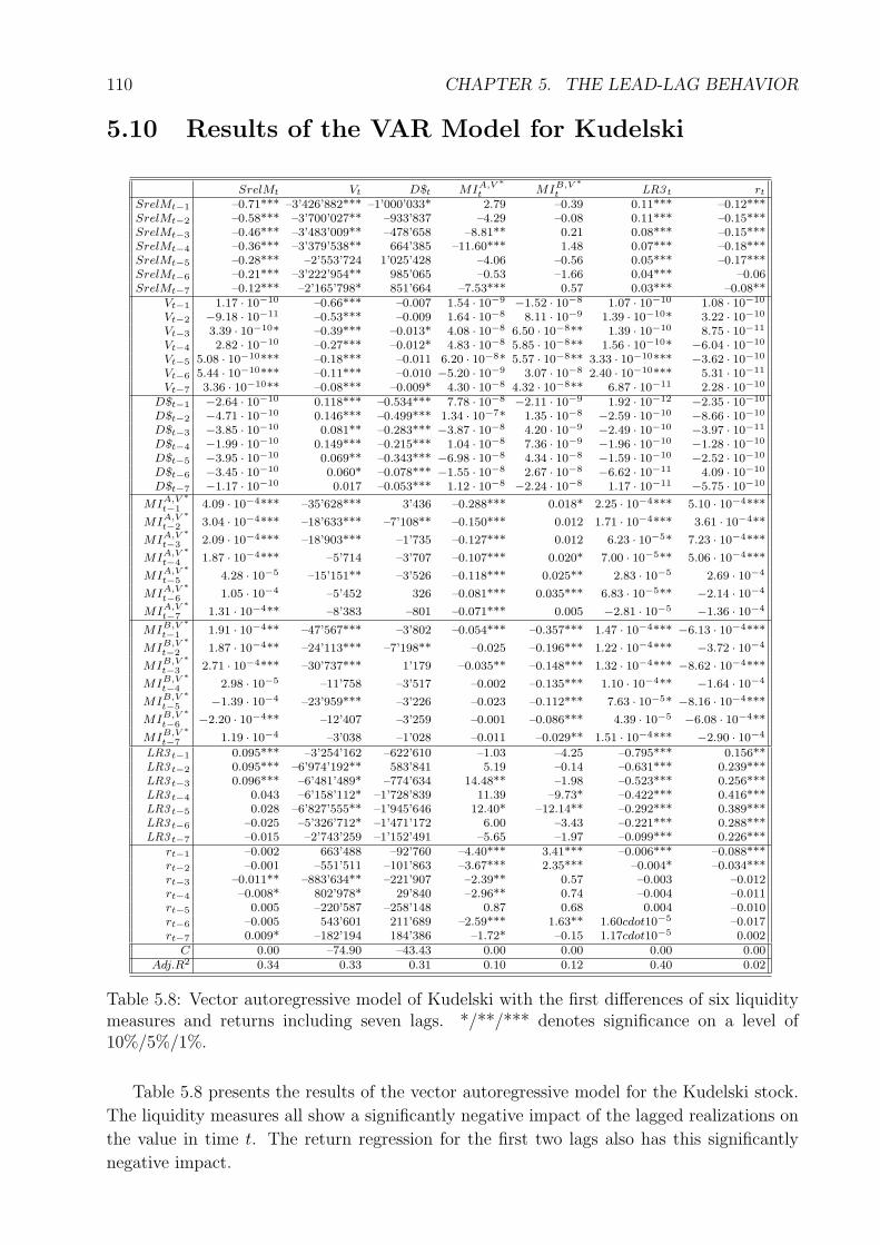
110 CHAPTER 5. THE LEAD-LAG BEHAVIOR
5.10 Results of the VAR Model for Kudelski
SrelMt Vt D$t MIA,V ∗t MIB,V ∗
t LR3 t rt
SrelMt−1 –0.71*** –3’426’882*** –1’000’033* 2.79 –0.39 0.11*** –0.12***SrelMt−2 –0.58*** –3’700’027** –933’837 –4.29 –0.08 0.11*** –0.15***SrelMt−3 –0.46*** –3’483’009** –478’658 –8.81** 0.21 0.08*** –0.15***SrelMt−4 –0.36*** –3’379’538** 664’385 –11.60*** 1.48 0.07*** –0.18***SrelMt−5 –0.28*** –2’553’724 1’025’428 –4.06 –0.56 0.05*** –0.17***SrelMt−6 –0.21*** –3’222’954** 985’065 –0.53 –1.66 0.04*** –0.06SrelMt−7 –0.12*** –2’165’798* 851’664 –7.53*** 0.57 0.03*** –0.08**
Vt−1 1.17 · 10−10 –0.66*** –0.007 1.54 · 10−9 −1.52 · 10−8 1.07 · 10−10 1.08 · 10−10
Vt−2 −9.18 · 10−11 –0.53*** –0.009 1.64 · 10−8 8.11 · 10−9 1.39 · 10−10* 3.22 · 10−10
Vt−3 3.39 · 10−10* –0.39*** –0.013* 4.08 · 10−8 6.50 · 10−8** 1.39 · 10−10 8.75 · 10−11
Vt−4 2.82 · 10−10 –0.27*** –0.012* 4.83 · 10−8 5.85 · 10−8** 1.56 · 10−10* −6.04 · 10−10
Vt−5 5.08 · 10−10*** –0.18*** –0.011 6.20 · 10−8* 5.57 · 10−8** 3.33 · 10−10*** −3.62 · 10−10
Vt−6 5.44 · 10−10*** –0.11*** –0.010 −5.20 · 10−9 3.07 · 10−8 2.40 · 10−10*** 5.31 · 10−11
Vt−7 3.36 · 10−10** –0.08*** –0.009* 4.30 · 10−8 4.32 · 10−8** 6.87 · 10−11 2.28 · 10−10
D$t−1 −2.64 · 10−10 0.118*** –0.534*** 7.78 · 10−8 −2.11 · 10−9 1.92 · 10−12 −2.35 · 10−10
D$t−2 −4.71 · 10−10 0.146*** –0.499*** 1.34 · 10−7* 1.35 · 10−8 −2.59 · 10−10 −8.66 · 10−10
D$t−3 −3.85 · 10−10 0.081** –0.283*** −3.87 · 10−8 4.20 · 10−9 −2.49 · 10−10 −3.97 · 10−11
D$t−4 −1.99 · 10−10 0.149*** –0.215*** 1.04 · 10−8 7.36 · 10−9 −1.96 · 10−10 −1.28 · 10−10
D$t−5 −3.95 · 10−10 0.069** –0.343*** −6.98 · 10−8 4.34 · 10−8 −1.59 · 10−10 −2.52 · 10−10
D$t−6 −3.45 · 10−10 0.060* –0.078*** −1.55 · 10−8 2.67 · 10−8 −6.62 · 10−11 4.09 · 10−10
D$t−7 −1.17 · 10−10 0.017 –0.053*** 1.12 · 10−8 −2.24 · 10−8 1.17 · 10−11 −5.75 · 10−10
MIA,V ∗t−1 4.09 · 10−4*** –35’628*** 3’436 –0.288*** 0.018* 2.25 · 10−4*** 5.10 · 10−4***
MIA,V ∗t−2 3.04 · 10−4*** –18’633*** –7’108** –0.150*** 0.012 1.71 · 10−4*** 3.61 · 10−4**
MIA,V ∗t−3 2.09 · 10−4*** –18’903*** –1’735 –0.127*** 0.012 6.23 · 10−5* 7.23 · 10−4***
MIA,V ∗t−4 1.87 · 10−4*** –5’714 –3’707 –0.107*** 0.020* 7.00 · 10−5** 5.06 · 10−4***
MIA,V ∗t−5 4.28 · 10−5 –15’151** –3’526 –0.118*** 0.025** 2.83 · 10−5 2.69 · 10−4
MIA,V ∗t−6 1.05 · 10−4 –5’452 326 –0.081*** 0.035*** 6.83 · 10−5** −2.14 · 10−4
MIA,V ∗t−7 1.31 · 10−4** –8’383 –801 –0.071*** 0.005 −2.81 · 10−5 −1.36 · 10−4
MIB,V ∗t−1 1.91 · 10−4** –47’567*** –3’802 –0.054*** –0.357*** 1.47 · 10−4*** −6.13 · 10−4***
MIB,V ∗t−2 1.87 · 10−4** –24’113*** –7’198** –0.025 –0.196*** 1.22 · 10−4*** −3.72 · 10−4
MIB,V ∗t−3 2.71 · 10−4*** –30’737*** 1’179 –0.035** –0.148*** 1.32 · 10−4*** −8.62 · 10−4***
MIB,V ∗t−4 2.98 · 10−5 –11’758 –3’517 –0.002 –0.135*** 1.10 · 10−4** −1.64 · 10−4
MIB,V ∗t−5 −1.39 · 10−4 –23’959*** –3’226 –0.023 –0.112*** 7.63 · 10−5* −8.16 · 10−4***
MIB,V ∗t−6 −2.20 · 10−4** –12’407 –3’259 –0.001 –0.086*** 4.39 · 10−5 −6.08 · 10−4**
MIB,V ∗t−7 1.19 · 10−4 –3’038 –1’028 –0.011 –0.029** 1.51 · 10−4*** −2.90 · 10−4
LR3 t−1 0.095*** –3’254’162 –622’610 –1.03 –4.25 –0.795*** 0.156**LR3 t−2 0.095*** –6’974’192** 583’841 5.19 –0.14 –0.631*** 0.239***LR3 t−3 0.096*** –6’481’489* –774’634 14.48** –1.98 –0.523*** 0.256***LR3 t−4 0.043 –6’158’112* –1’728’839 11.39 –9.73* –0.422*** 0.416***LR3 t−5 0.028 –6’827’555** –1’945’646 12.40* –12.14** –0.292*** 0.389***LR3 t−6 –0.025 –5’326’712* –1’471’172 6.00 –3.43 –0.221*** 0.288***LR3 t−7 –0.015 –2’743’259 –1’152’491 –5.65 –1.97 –0.099*** 0.226***
rt−1 –0.002 663’488 –92’760 –4.40*** 3.41*** –0.006*** –0.088***rt−2 –0.001 –551’511 –101’863 –3.67*** 2.35*** –0.004* –0.034***rt−3 –0.011** –883’634** –221’907 –2.39** 0.57 –0.003 –0.012rt−4 –0.008* 802’978* 29’840 –2.96** 0.74 –0.004 –0.011rt−5 0.005 –220’587 –258’148 0.87 0.68 0.004 –0.010rt−6 –0.005 543’601 211’689 –2.59*** 1.63** 1.60cdot10−5 –0.017rt−7 0.009* –182’194 184’386 –1.72* –0.15 1.17cdot10−5 0.002
C 0.00 –74.90 –43.43 0.00 0.00 0.00 0.00Adj.R2 0.34 0.33 0.31 0.10 0.12 0.40 0.02
Table 5.8: Vector autoregressive model of Kudelski with the first differences of six liquiditymeasures and returns including seven lags. */**/*** denotes significance on a level of10%/5%/1%.
Table 5.8 presents the results of the vector autoregressive model for the Kudelski stock.
The liquidity measures all show a significantly negative impact of the lagged realizations on
the value in time t. The return regression for the first two lags also has this significantly
negative impact.
5.10. RESULTS OF THE VAR MODEL FOR KUDELSKI 111
The interrelation of lagged turnover and the relative spread is positive but only significant
for lags three and five to seven. Lagged dollar depth does not influence the relative spread,
and the opposite regression of dollar depth on lagged spreads shows a slightly negative
significance at lag one. The relative spread is positively influenced by the market impact on
the ask-side on lags one to four and seven. For lags up to three the market impact on the
bid-side has a positive impact on the relative spread. Also the coefficient of lag six is negative
and significant. As for the Holcim stock, Kudelski shows a significantly positive impact of
the first three lagged liquidity ratios 3 on the relative spread. The impact of lagged returns
on the relative spread is negative and significant for lags three and four. There is a slightly
positive impact of the coefficient at lag seven.
Rising spreads lead to smaller turnovers with significance on all lags, with exception of
lag five which cannot be distinguished from zero. Dollar depth of lags up to six is followed
by rising turnover. The market impact measures let turnover decline with significance for
lags one to three and five. Also, declining liquidity, as measured by the liquidity ratio 3,
leads to a declining turnover. There is significance for lags two to six. The impact of returns
on turnover is ambiguous: return in t − 3 has a significantly negative impact on turnover
while on lag four the connection is positive and significant on the 10% level.
Dollar depth is slightly negatively influenced by turnovers of lags three, four and seven.
The market impact measures (both on lag two) have a negative impact on dollar depth.
The lagged liquidity ratios 3 and the lagged returns do not influence dollar depth. The
opposite also holds: Lagged dollar depth does not significantly change the liquidity ratio 3
and returns.
The lagged relative spread is followed by a declining market impact on the ask-side. The
significantly negative coefficients show up at lags three, four and seven. Turnover and depth
lead to positive changes of the market impact on the ask-side with only slight significance
on lags five and two. The significant coefficients of market impact on the bid-side have a
negative effect on market impact on the ask-side. Lags three and five of the liquidity ratio 3
lead to a rise in the market impact on the ask-side. Almost all lagged returns significantly
reduce the market impact on the ask-side.
Market impact on the bid-side is not changed by the lagged relative spread. As for the
ask-side, turnover leads to a rising market impact on the bid-side, since the coefficients of
lags three to five and seven are significantly different from zero. Dollar depth has no influence
on market impact on the ask-side. The market impact on the ask-side of the order book
leads to a declining market impact on the bid-side as lags one and four to six show. The
impact of the liquidity ratio 3 with respect to the market impact on the bid-side is negative
for Kudelski on lags four and five. The lagged returns lead to higher market impacts on the
bid-side, as expected, with significance on lags one, two and six.
The liquidity ratio 3 is significantly positively influenced by the relative spread on all
lags. Turnover leads to a higher liquidity ratio 3 on lags two and four to six. Market impact
on the ask-side and market impact on the bid-side lead both to a higher liquidity ratio 3
with significance for almost all lags. Declining stock prices of lags one and two are followed
by a rising liquidity ratio 3.
Almost all lags of the relative spread lead to lower stock prices, while lagged turnover
does not influence returns. The significant market impact on the ask-side coefficients are
112 CHAPTER 5. THE LEAD-LAG BEHAVIOR
followed by higher returns, while the market impact on the bid-side leads to smaller returns.
In contrast to the other stocks so far, all the lagged coefficients of the liquidity ratio 3 are
significantly positive.
None of the constants of the model is significantly different from zero and the adjusted
R2-values are in the range of the previous stocks.
5.11 Results of the VAR Model for Lonza
Table 5.9 presents the results of the vector autoregressive model for Lonza. Also for this
stock, the liquidity measures depend on all their own lags significantly negatively.
Rising turnover of lags up to six lead to larger relative spreads. Lagged dollar depth does
not influence the relative spread. The influence of lagged market impacts on the ask-side on
returns is ambiguous: for lags one and two it is significantly positive while for lags five to
seven it is significantly negative. The market impact on the bid-side is followed on lags two,
four and five by a rising relative spread. The liquidity ratio 3 has a positive impact on the
relative spread. The first two lags are significant. Rising stock prices in t− 1 and t− 2 lead
to a rising relative spread. On lags four and seven the impact is significantly negative.
The relative spread on lags up to three makes turnover decline. Rising dollar depth
leads to higher turnover with significance for all lags. The influence of the market impact
measures on turnover is negative, but only lags one and two on the ask-side and lag seven
on the bid-side are significantly different from zero. The lagged liquidity ratio 3 does not
change turnover significantly and, also, in the other direction from lagged turnovers to the
liquidity ratio 3 no interrelation is found. Lagged returns on lag three and seven lead to
significantly lower turnovers.
A rising spread of lags up to six leads to a significantly lower dollar depth. Lagged
turnover does not influence dollar depth. For the market impact measures there is no con-
nection to dollar depth and, also, the opposite holds: lagged dollar depth does not influence
the market impact measures. The lagged liquidity ratio 3 and lagged return do not have any
impact on dollar depth. Again, dollar depth neither influences the liquidity ratio 3 nor the
return.
The market impact on the ask-side is positively influenced by the lagged relative spread.
Almost all coefficients are significant. Turnover does not influence the market impact mea-
sures, neither on the bid- nor on the ask-side. The market impact on the bid-side leads to a
higher market impact on the ask-side with significance for lags four and five. This in contrast
to the Kudelski stock, for example. The lagged liquidity ratio 3 in time t− 1 and t− 2 leads
to a significantly lower market impact on the ask-side. Rising stock prices of lags one, five
and six are followed by a declining market impact on the ask-side while on lag three there
is a slightly positive impact.
The significant coefficients of the lagged relative spread show a negative relation to mar-
ket impact on the bid-side. Market impact on the ask-side does not lead to any significant
changes in market impact on the bid-side. Lag five of the liquidity ratio 3 shows a signifi-
cantly positive impact on the market impact on the bid-side. The coefficients of the lagged
returns are significantly positive on lags three to five. The return of lag two is negative on
a significance level of 10%.
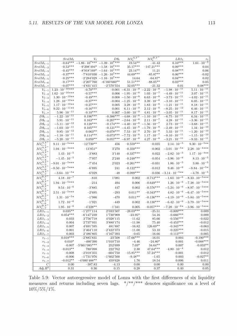
5.11. RESULTS OF THE VAR MODEL FOR LONZA 113
SrelMt Vt D$t MIA,V ∗t MIB,V ∗
t LR3 t rt
SrelMt−1 –0.64*** −1.86 · 107*** −1.39 · 107*** 19.54** –41.42 0.10*** 1.61 · 10−3
SrelMt−2 –0.53*** –9’298’494* −1.58 · 107*** 35.17*** –147.21*** 0.09*** 0.04SrelMt−3 –0.45*** –8’918’169* −1.64 · 107*** 23.14** 11.21 0.08*** 0.06SrelMt−4 –0.37*** –7’810’030 −1.26 · 107*** 44.69*** –85.87** 0.06*** –0.02SrelMt−5 –0.25*** –2’284’029 −1.16 · 107*** 14.64 –64.87* 0.04*** 0.02SrelMt−6 –0.17*** –2’207’760 –6’160’660** 51.51*** –88.05** 0.03*** 0.05SrelMt−7 –0.07*** –4’831’415 –2’570’554 32.05*** –21.32 0.01 0.08***
Vt−1 1.23 · 10−10*** –0.70*** –0.001 −6.31 · 10−9 −2.22 · 10−8 −1.98 · 10−11 5.11 · 10−11
Vt−2 1.62 · 10−10*** –0.57*** 0.006 −1.95 · 10−8 1.03 · 10−7 −4.49 · 10−11 3.07 · 10−11
Vt−3 1.30 · 10−10** –0.49*** 0.008 −1.50 · 10−8 6.63 · 10−8 −3.73 · 10−11 −4.02 · 10−11
Vt−4 1.28 · 10−10** –0.37*** –0.004 −1.25 · 10−8 3.39 · 10−8 −3.10 · 10−11 6.05 · 10−11
Vt−5 1.17 · 10−10** –0.27*** 0.005 3.28 · 10−9 1.83 · 10−8 −1.21 · 10−11 8.18 · 10−11
Vt−6 9.22 · 10−11** –0.16*** 0.001 6.11 · 10−9 2.12 · 10−8 −8.25 · 10−12 6.46 · 10−11
Vt−7 5.96 · 10−11 –0.10*** 0.007 −3.60 · 10−9 4.81 · 10−8 −3.05 · 10−11 8.17 · 10−11
D$t−1 −1.22 · 10−11 0.196*** –0.386*** −4.68 · 10−8 −1.10 · 10−7 −6.75 · 10−11 6.34 · 10−11
D$t−2 5.91 · 10−11 0.163*** –0.207*** −2.64 · 10−8 2.11 · 10−7 4.28 · 10−11 −3.36 · 10−11
D$t−3 −5.11 · 10−12 0.128*** –0.174*** −4.40 · 10−8 −1.56 · 10−7 2.73 · 10−11 −3.68 · 10−11
D$t−4 −1.03 · 10−11 0.105*** –0.121*** −4.45 · 10−8 −1.79 · 10−8 −2.49 · 10−11 1.34 · 10−10
D$t−5 9.85 · 10−12 0.063** –0.078*** 7.53 · 10−9 2.70 · 10−8 5.33 · 10−11 −1.20 · 10−10
D$t−6 −1.18 · 10−11 0.114*** –0.073*** −7.72 · 10−8 1.17 · 10−7 −8.10 · 10−11 −1.15 · 10−10
D$t−7 −5.20 · 10−11 0.059** –0.057*** −6.97 · 10−8 4.27 · 10−8 −3.21 · 10−11 −9.33 · 10−11
MIA,V ∗t−1 9.11 · 10−5*** –12’739** 456 –0.559*** –0.035 2.14 · 10−5 9.30 · 10−5**
MIA,V ∗t−2 1.04 · 10−4*** –13’851* 3’270 –0.350*** –0.002 −3.01 · 10−5* 2.28 · 10−4***
MIA,V ∗t−3 1.43 · 10−5 –3’883 3’140 –0.337*** 0.022 −2.82 · 10−5 1.17 · 10−4**
MIA,V ∗t−4 −1.45 · 10−5 –7’957 2’240 –0.248*** –0.054 −3.96 · 10−6 8.13 · 10−5
MIA,V ∗t−5 −9.01 · 10−5*** –7’454 2’023 –0.261*** –0.031 1.86 · 10−5 3.88 · 10−5
MIA,V ∗t−6 −8.50 · 10−5*** –6’895 241 –0.122*** –0.012 9.46 · 10−6 −8.84 · 10−5*
MIA,V ∗t−7 −3.64 · 10−5* –6’029 –48 –0.099*** –0.036 −3.14 · 10−5** −4.78 · 10−5
MIB,V ∗t−1 4.18 · 10−7 –810 1’081 0.002 –0.712*** −1.63 · 10−6 −8.33 · 10−5***
MIB,V ∗t−2 1.94 · 10−5*** –214 494 0.006 –0.649*** 1.26 · 10−6 −7.38 · 10−5***
MIB,V ∗t−3 9.54 · 10−6 –3’885 447 0.002 –0.576*** −5.24 · 10−6 −8.97 · 10−5***
MIB,V ∗t−4 2.51 · 10−5*** –2’695 –293 0.011** –0.343*** 4.82 · 10−6 −6.47 · 10−5***
MIB,V ∗t−5 1.31 · 10−5* –1’986 –470 0.011** –0.136*** −4.19 · 10−6 −5.84 · 10−5***
MIB,V ∗t−6 1.72 · 10−6 –1’921 –449 0.002 –0.130*** −6.42 · 10−6 −3.79 · 10−5***
MIB,V ∗t−7 1.95 · 10−6 –4’228** –1’341 0.005 –0.057*** −7.28 · 10−6* −3.96 · 10−5***
LR3 t−1 0.035** –1’277’114 2’033’507 –28.03*** –25.51 –0.809*** 0.009LR3 t−2 0.054*** –6’147’239 1’730’909 –23.95* 54.16 –0.666*** 0.009LR3 t−3 0.033 3’756’718 4’028’115 –11.62 85.66 –0.556*** –0.022LR3 t−4 0.004 2’737’931 3’880’174 –11.98 75.40 –0.453*** –0.012LR3 t−5 0.007 4’691’595 481’887 –16.82 126.69** –0.345*** –0.063LR3 t−6 0.001 2’464’110 –2’422’373 –11.00 53.10 –0.225*** –0.015LR3 t−7 0.003 2’486’805 –4’167’393 –0.65 –16.66 –0.113*** –0.005
rt−1 0.018*** –2’885’831 –23’508 –17.66*** –16.01 0.004 –0.190***rt−2 0.010* –490’390 1’010’710 –4.46 –24.80* 0.001 –0.088***rt−3 –0.007 –5’661’085*** 252’699 7.03* 34.64** 0.007 –0.033**rt−4 –0.013** 788’098 222’762 2.30 47.64*** –4.80 · 10−4 0.012rt−5 –0.008 –2’018’355 –604’750 –15.85*** 57.24*** –0.001 –0.012rt−6 –0.006 –1’731’976 –1’602’500 –9.48** –1.65 0.003 –0.027**rt−7 –0.012** –4’000’488** 459’628 1.76 18.54 0.006 0.011
C 0.00 –387.83 –4.13 0.00 0.00 0.00 0.00Adj.R2 0.31 0.36 0.15 0.28 0.37 0.40 0.05
Table 5.9: Vector autoregressive model of Lonza with the first differences of six liquiditymeasures and returns including seven lags. */**/*** denotes significance on a level of10%/5%/1%.
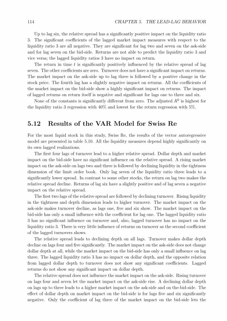
114 CHAPTER 5. THE LEAD-LAG BEHAVIOR
Up to lag six, the relative spread has a significantly positive impact on the liquidity ratio
3. The significant coefficients of the lagged market impact measures with respect to the
liquidity ratio 3 are all negative. They are significant for lag two and seven on the ask-side
and for lag seven on the bid-side. Returns are not able to predict the liquidity ratio 3 and
vice versa; the lagged liquidity ratios 3 have no impact on return.
The return in time t is significantly positively influenced by the relative spread of lag
seven. The other coefficients are zero. Turnover does not have a significant impact on returns.
The market impact on the ask-side up to lag three is followed by a positive change in the
stock price. The fourth lag has a slightly negative impact on returns. All the coefficients of
the market impact on the bid-side show a highly significant impact on returns. The impact
of lagged returns on return itself is negative and significant for lags one to three and six.
None of the constants is significantly different from zero. The adjusted R2 is highest for
the liquidity ratio 3 regression with 40% and lowest for the return regression with 5%.
5.12 Results of the VAR Model for Swiss Re
For the most liquid stock in this study, Swiss Re, the results of the vector autoregressive
model are presented in table 5.10. All the liquidity measures depend highly significantly on
its own lagged realizations.
The first four lags of turnover lead to a higher relative spread. Dollar depth and market
impact on the bid-side have no significant influence on the relative spread. A rising market
impact on the ask-side on lags two and three is followed by declining liquidity in the tightness
dimension of the limit order book. Only lag seven of the liquidity ratio three leads to a
significantly lower spread. In contrast to some other stocks, the return on lag two makes the
relative spread decline. Returns of lag six have a slightly positive and of lag seven a negative
impact on the relative spread.
The first two lags of the relative spread are followed by declining turnover. Rising liquidity
in the tightness and depth dimension leads to higher turnover. The market impact on the
ask-side makes turnover decline, as lags one, five and six show. The market impact on the
bid-side has only a small influence with the coefficient for lag one. The lagged liquidity ratio
3 has no significant influence on turnover and, also, lagged turnover has no impact on the
liquidity ratio 3. There is very little influence of returns on turnover as the second coefficient
of the lagged turnovers shows.
The relative spread leads to declining depth on all lags. Turnover makes dollar depth
decline on lags four and five significantly. The market impact on the ask-side does not change
dollar depth at all, while the market impact on the bid-side has only a small influence on lag
three. The lagged liquidity ratio 3 has no impact on dollar depth, and the opposite relation
from lagged dollar depth to turnover does not show any significant coefficients. Lagged
returns do not show any significant impact on dollar depth.
The relative spread does not influence the market impact on the ask-side. Rising turnover
on lags four and seven let the market impact on the ask-side rise. A declining dollar depth
on lags up to three leads to a higher market impact on the ask-side and on the-bid-side. The
effect of dollar depth on market impact on the bid-side is for lags five and six significantly
negative. Only the coefficient of lag three of the market impact on the bid-side lets the
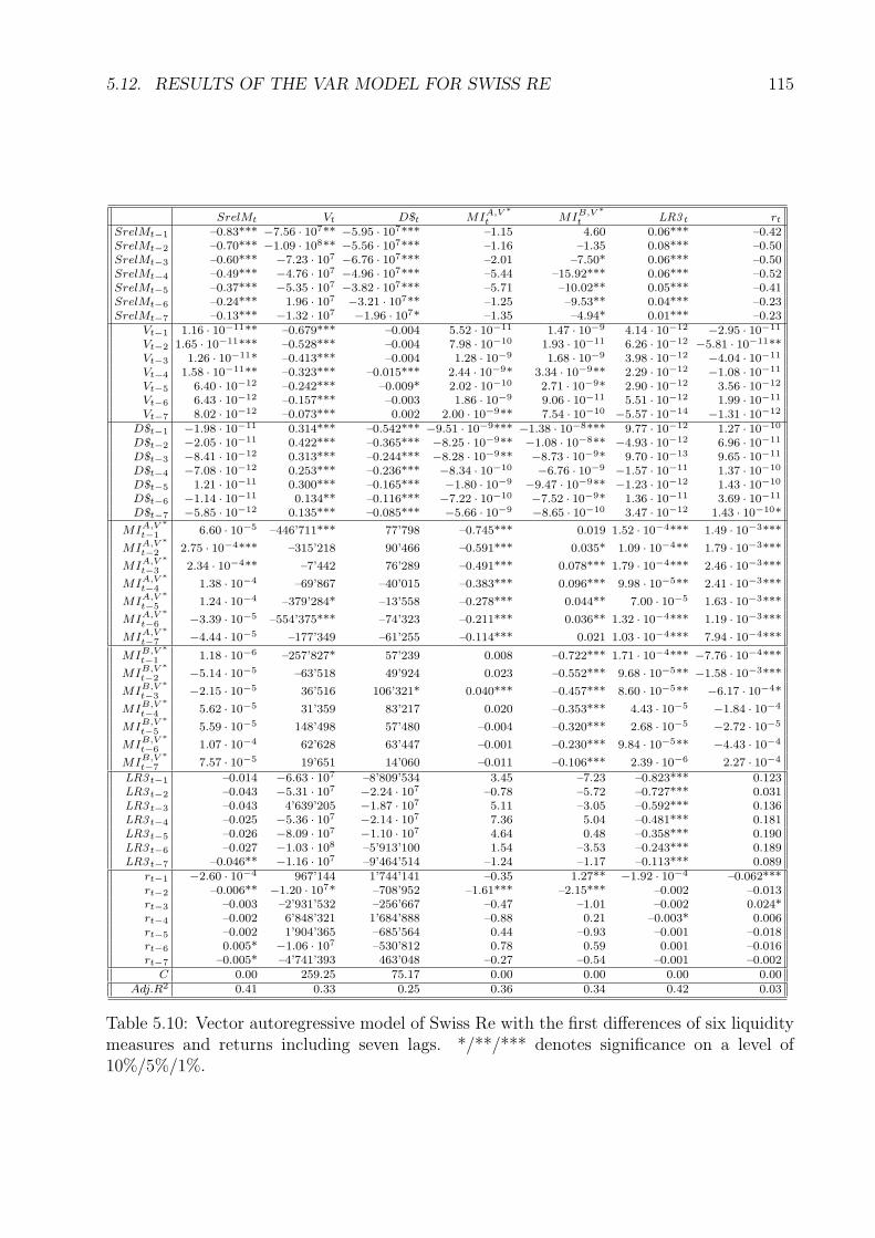
5.12. RESULTS OF THE VAR MODEL FOR SWISS RE 115
SrelMt Vt D$t MIA,V ∗t MIB,V ∗
t LR3 t rt
SrelMt−1 –0.83*** −7.56 · 107** −5.95 · 107*** –1.15 4.60 0.06*** –0.42SrelMt−2 –0.70*** −1.09 · 108** −5.56 · 107*** –1.16 –1.35 0.08*** –0.50SrelMt−3 –0.60*** −7.23 · 107 −6.76 · 107*** –2.01 –7.50* 0.06*** –0.50SrelMt−4 –0.49*** −4.76 · 107 −4.96 · 107*** –5.44 –15.92*** 0.06*** –0.52SrelMt−5 –0.37*** −5.35 · 107 −3.82 · 107*** –5.71 –10.02** 0.05*** –0.41SrelMt−6 –0.24*** 1.96 · 107 −3.21 · 107** –1.25 –9.53** 0.04*** –0.23SrelMt−7 –0.13*** −1.32 · 107 −1.96 · 107* –1.35 –4.94* 0.01*** –0.23
Vt−1 1.16 · 10−11** –0.679*** –0.004 5.52 · 10−11 1.47 · 10−9 4.14 · 10−12 −2.95 · 10−11
Vt−2 1.65 · 10−11*** –0.528*** –0.004 7.98 · 10−10 1.93 · 10−11 6.26 · 10−12 −5.81 · 10−11**Vt−3 1.26 · 10−11* –0.413*** –0.004 1.28 · 10−9 1.68 · 10−9 3.98 · 10−12 −4.04 · 10−11
Vt−4 1.58 · 10−11** –0.323*** –0.015*** 2.44 · 10−9* 3.34 · 10−9** 2.29 · 10−12 −1.08 · 10−11
Vt−5 6.40 · 10−12 –0.242*** –0.009* 2.02 · 10−10 2.71 · 10−9* 2.90 · 10−12 3.56 · 10−12
Vt−6 6.43 · 10−12 –0.157*** –0.003 1.86 · 10−9 9.06 · 10−11 5.51 · 10−12 1.99 · 10−11
Vt−7 8.02 · 10−12 –0.073*** 0.002 2.00 · 10−9** 7.54 · 10−10 −5.57 · 10−14 −1.31 · 10−12
D$t−1 −1.98 · 10−11 0.314*** –0.542*** −9.51 · 10−9*** −1.38 · 10−8*** 9.77 · 10−12 1.27 · 10−10
D$t−2 −2.05 · 10−11 0.422*** –0.365*** −8.25 · 10−9** −1.08 · 10−8** −4.93 · 10−12 6.96 · 10−11
D$t−3 −8.41 · 10−12 0.313*** –0.244*** −8.28 · 10−9** −8.73 · 10−9* 9.70 · 10−13 9.65 · 10−11
D$t−4 −7.08 · 10−12 0.253*** –0.236*** −8.34 · 10−10 −6.76 · 10−9 −1.57 · 10−11 1.37 · 10−10
D$t−5 1.21 · 10−11 0.300*** –0.165*** −1.80 · 10−9 −9.47 · 10−9** −1.23 · 10−12 1.43 · 10−10
D$t−6 −1.14 · 10−11 0.134** –0.116*** −7.22 · 10−10 −7.52 · 10−9* 1.36 · 10−11 3.69 · 10−11
D$t−7 −5.85 · 10−12 0.135*** –0.085*** −5.66 · 10−9 −8.65 · 10−10 3.47 · 10−12 1.43 · 10−10*
MIA,V ∗t−1 6.60 · 10−5 –446’711*** 77’798 –0.745*** 0.019 1.52 · 10−4*** 1.49 · 10−3***
MIA,V ∗t−2 2.75 · 10−4*** –315’218 90’466 –0.591*** 0.035* 1.09 · 10−4** 1.79 · 10−3***
MIA,V ∗t−3 2.34 · 10−4** –7’442 76’289 –0.491*** 0.078*** 1.79 · 10−4*** 2.46 · 10−3***
MIA,V ∗t−4 1.38 · 10−4 –69’867 –40’015 –0.383*** 0.096*** 9.98 · 10−5** 2.41 · 10−3***
MIA,V ∗t−5 1.24 · 10−4 –379’284* –13’558 –0.278*** 0.044** 7.00 · 10−5 1.63 · 10−3***
MIA,V ∗t−6 −3.39 · 10−5 –554’375*** –74’323 –0.211*** 0.036** 1.32 · 10−4*** 1.19 · 10−3***
MIA,V ∗t−7 −4.44 · 10−5 –177’349 –61’255 –0.114*** 0.021 1.03 · 10−4*** 7.94 · 10−4***
MIB,V ∗t−1 1.18 · 10−6 –257’827* 57’239 0.008 –0.722*** 1.71 · 10−4*** −7.76 · 10−4***
MIB,V ∗t−2 −5.14 · 10−5 –63’518 49’924 0.023 –0.552*** 9.68 · 10−5** −1.58 · 10−3***
MIB,V ∗t−3 −2.15 · 10−5 36’516 106’321* 0.040*** –0.457*** 8.60 · 10−5** −6.17 · 10−4*
MIB,V ∗t−4 5.62 · 10−5 31’359 83’217 0.020 –0.353*** 4.43 · 10−5 −1.84 · 10−4
MIB,V ∗t−5 5.59 · 10−5 148’498 57’480 –0.004 –0.320*** 2.68 · 10−5 −2.72 · 10−5
MIB,V ∗t−6 1.07 · 10−4 62’628 63’447 –0.001 –0.230*** 9.84 · 10−5** −4.43 · 10−4
MIB,V ∗t−7 7.57 · 10−5 19’651 14’060 –0.011 –0.106*** 2.39 · 10−6 2.27 · 10−4
LR3 t−1 –0.014 −6.63 · 107 –8’809’534 3.45 –7.23 –0.823*** 0.123LR3 t−2 –0.043 −5.31 · 107 −2.24 · 107 –0.78 –5.72 –0.727*** 0.031LR3 t−3 –0.043 4’639’205 −1.87 · 107 5.11 –3.05 –0.592*** 0.136LR3 t−4 –0.025 −5.36 · 107 −2.14 · 107 7.36 5.04 –0.481*** 0.181LR3 t−5 –0.026 −8.09 · 107 −1.10 · 107 4.64 0.48 –0.358*** 0.190LR3 t−6 –0.027 −1.03 · 108 –5’913’100 1.54 –3.53 –0.243*** 0.189LR3 t−7 –0.046** −1.16 · 107 –9’464’514 –1.24 –1.17 –0.113*** 0.089
rt−1 −2.60 · 10−4 967’144 1’744’141 –0.35 1.27** −1.92 · 10−4 –0.062***rt−2 –0.006** −1.20 · 107* –708’952 –1.61*** –2.15*** –0.002 –0.013rt−3 –0.003 –2’931’532 –256’667 –0.47 –1.01 –0.002 0.024*rt−4 –0.002 6’848’321 1’684’888 –0.88 0.21 –0.003* 0.006rt−5 –0.002 1’904’365 –685’564 0.44 –0.93 –0.001 –0.018rt−6 0.005* −1.06 · 107 –530’812 0.78 0.59 0.001 –0.016rt−7 –0.005* –4’741’393 463’048 –0.27 –0.54 –0.001 –0.002
C 0.00 259.25 75.17 0.00 0.00 0.00 0.00Adj.R2 0.41 0.33 0.25 0.36 0.34 0.42 0.03
Table 5.10: Vector autoregressive model of Swiss Re with the first differences of six liquiditymeasures and returns including seven lags. */**/*** denotes significance on a level of10%/5%/1%.
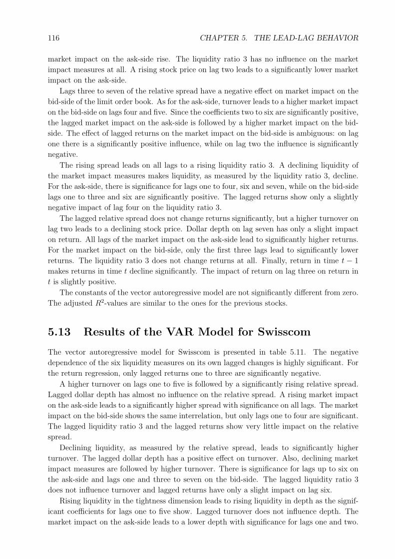
116 CHAPTER 5. THE LEAD-LAG BEHAVIOR
market impact on the ask-side rise. The liquidity ratio 3 has no influence on the market
impact measures at all. A rising stock price on lag two leads to a significantly lower market
impact on the ask-side.
Lags three to seven of the relative spread have a negative effect on market impact on the
bid-side of the limit order book. As for the ask-side, turnover leads to a higher market impact
on the bid-side on lags four and five. Since the coefficients two to six are significantly positive,
the lagged market impact on the ask-side is followed by a higher market impact on the bid-
side. The effect of lagged returns on the market impact on the bid-side is ambiguous: on lag
one there is a significantly positive influence, while on lag two the influence is significantly
negative.
The rising spread leads on all lags to a rising liquidity ratio 3. A declining liquidity of
the market impact measures makes liquidity, as measured by the liquidity ratio 3, decline.
For the ask-side, there is significance for lags one to four, six and seven, while on the bid-side
lags one to three and six are significantly positive. The lagged returns show only a slightly
negative impact of lag four on the liquidity ratio 3.
The lagged relative spread does not change returns significantly, but a higher turnover on
lag two leads to a declining stock price. Dollar depth on lag seven has only a slight impact
on return. All lags of the market impact on the ask-side lead to significantly higher returns.
For the market impact on the bid-side, only the first three lags lead to significantly lower
returns. The liquidity ratio 3 does not change returns at all. Finally, return in time t − 1
makes returns in time t decline significantly. The impact of return on lag three on return in
t is slightly positive.
The constants of the vector autoregressive model are not significantly different from zero.
The adjusted R2-values are similar to the ones for the previous stocks.
5.13 Results of the VAR Model for Swisscom
The vector autoregressive model for Swisscom is presented in table 5.11. The negative
dependence of the six liquidity measures on its own lagged changes is highly significant. For
the return regression, only lagged returns one to three are significantly negative.
A higher turnover on lags one to five is followed by a significantly rising relative spread.
Lagged dollar depth has almost no influence on the relative spread. A rising market impact
on the ask-side leads to a significantly higher spread with significance on all lags. The market
impact on the bid-side shows the same interrelation, but only lags one to four are significant.
The lagged liquidity ratio 3 and the lagged returns show very little impact on the relative
spread.
Declining liquidity, as measured by the relative spread, leads to significantly higher
turnover. The lagged dollar depth has a positive effect on turnover. Also, declining market
impact measures are followed by higher turnover. There is significance for lags up to six on
the ask-side and lags one and three to seven on the bid-side. The lagged liquidity ratio 3
does not influence turnover and lagged returns have only a slight impact on lag six.
Rising liquidity in the tightness dimension leads to rising liquidity in depth as the signif-
icant coefficients for lags one to five show. Lagged turnover does not influence depth. The
market impact on the ask-side leads to a lower depth with significance for lags one and two.
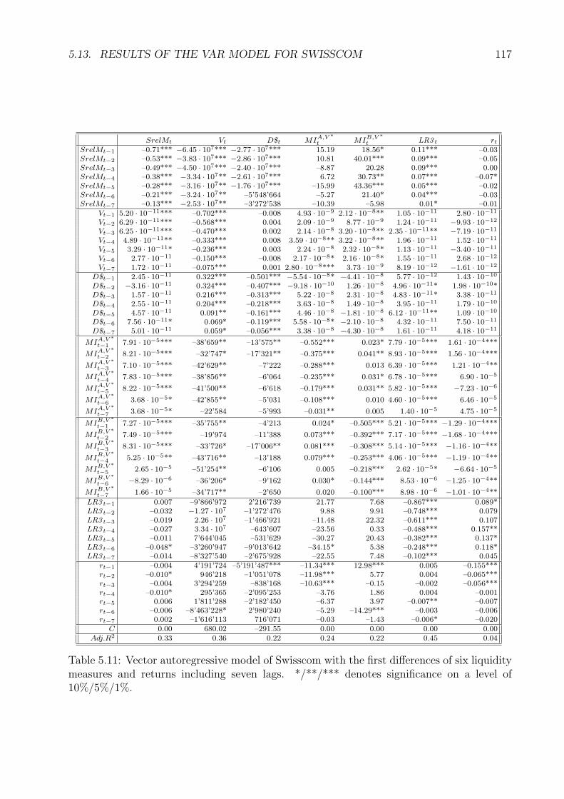
5.13. RESULTS OF THE VAR MODEL FOR SWISSCOM 117
SrelMt Vt D$t MIA,V ∗t MIB,V ∗
t LR3 t rt
SrelMt−1 –0.71*** −6.45 · 107*** −2.77 · 107*** 15.19 18.56* 0.11*** –0.03SrelMt−2 –0.53*** −3.83 · 107*** −2.86 · 107*** 10.81 40.01*** 0.09*** –0.05SrelMt−3 –0.49*** −4.50 · 107*** −2.40 · 107*** –8.87 20.28 0.09*** 0.00SrelMt−4 –0.38*** −3.34 · 107** −2.61 · 107*** 6.72 30.73** 0.07*** –0.07*SrelMt−5 –0.28*** −3.16 · 107** −1.76 · 107*** –15.99 43.36*** 0.05*** –0.02SrelMt−6 –0.21*** −3.24 · 107** –5’548’664 –5.27 21.40* 0.04*** –0.03SrelMt−7 –0.13*** −2.53 · 107** –3’272’538 –10.39 –5.98 0.01* –0.01
Vt−1 5.20 · 10−11*** –0.702*** –0.008 4.93 · 10−9 2.12 · 10−8** 1.05 · 10−11 2.80 · 10−11
Vt−2 6.29 · 10−11*** –0.568*** 0.004 2.09 · 10−9 8.77 · 10−9 1.24 · 10−11 −9.93 · 10−12
Vt−3 6.25 · 10−11*** –0.470*** 0.002 2.14 · 10−8 3.20 · 10−8** 2.35 · 10−11** −7.19 · 10−11
Vt−4 4.89 · 10−11** –0.333*** 0.008 3.59 · 10−8** 3.22 · 10−8** 1.96 · 10−11 1.52 · 10−11
Vt−5 3.29 · 10−11* –0.236*** 0.003 2.24 · 10−8 2.32 · 10−8* 1.13 · 10−11 −3.40 · 10−11
Vt−6 2.77 · 10−11 –0.150*** –0.008 2.17 · 10−8* 2.16 · 10−8* 1.55 · 10−11 2.68 · 10−12
Vt−7 1.72 · 10−11 –0.075*** 0.001 2.80 · 10−8*** 3.73 · 10−9 8.19 · 10−12 −1.61 · 10−12
D$t−1 2.45 · 10−11 0.322*** –0.501*** −5.54 · 10−8* −4.41 · 10−8 5.77 · 10−12 1.43 · 10−10
D$t−2 −3.16 · 10−11 0.324*** –0.407*** −9.18 · 10−10 1.26 · 10−8 4.96 · 10−11* 1.98 · 10−10*D$t−3 1.57 · 10−11 0.216*** –0.313*** 5.22 · 10−8 2.31 · 10−8 4.83 · 10−11* 3.38 · 10−11
D$t−4 2.55 · 10−11 0.204*** –0.218*** 3.63 · 10−8 1.49 · 10−8 3.95 · 10−11 1.79 · 10−10
D$t−5 4.57 · 10−11 0.091** –0.161*** 4.46 · 10−8 −1.81 · 10−8 6.12 · 10−11** 1.09 · 10−10
D$t−6 7.56 · 10−11* 0.069* –0.119*** 5.58 · 10−8* −2.10 · 10−8 4.32 · 10−11 7.50 · 10−11
D$t−7 5.01 · 10−11 0.059* –0.056*** 3.38 · 10−8 −4.30 · 10−8 1.61 · 10−11 4.18 · 10−11
MIA,V ∗t−1 7.91 · 10−5*** –38’659** –13’575** –0.552*** 0.023* 7.79 · 10−5*** 1.61 · 10−4***
MIA,V ∗t−2 8.21 · 10−5*** –32’747* –17’321** –0.375*** 0.041** 8.93 · 10−5*** 1.56 · 10−4***
MIA,V ∗t−3 7.10 · 10−5*** –42’629** –7’222 –0.288*** 0.013 6.39 · 10−5*** 1.21 · 10−4**
MIA,V ∗t−4 7.83 · 10−5*** –38’856** –6’064 –0.235*** 0.031* 6.78 · 10−5*** 6.90 · 10−5
MIA,V ∗t−5 8.22 · 10−5*** –41’500** –6’618 –0.179*** 0.031** 5.82 · 10−5*** −7.23 · 10−6
MIA,V ∗t−6 3.68 · 10−5* –42’855** –5’031 –0.108*** 0.010 4.60 · 10−5*** 6.46 · 10−5
MIA,V ∗t−7 3.68 · 10−5* –22’584 –5’993 –0.031** 0.005 1.40 · 10−5 4.75 · 10−5
MIB,V ∗t−1 7.27 · 10−5*** –35’755** –4’213 0.024* –0.505*** 5.21 · 10−5*** −1.29 · 10−4***
MIB,V ∗t−2 7.49 · 10−5*** –19’974 –11’388 0.073*** –0.392*** 7.17 · 10−5*** −1.68 · 10−4***
MIB,V ∗t−3 8.31 · 10−5*** –33’726* –17’006** 0.081*** –0.308*** 5.14 · 10−5*** −1.16 · 10−4**
MIB,V ∗t−4 5.25 · 10−5** –43’716** –13’188 0.079*** –0.253*** 4.06 · 10−5*** −1.19 · 10−4**
MIB,V ∗t−5 2.65 · 10−5 –51’254** –6’106 0.005 –0.218*** 2.62 · 10−5* −6.64 · 10−5
MIB,V ∗t−6 −8.29 · 10−6 –36’206* –9’162 0.030* –0.144*** 8.53 · 10−6 −1.25 · 10−4**
MIB,V ∗t−7 1.66 · 10−5 –34’717** –2’650 0.020 –0.100*** 8.98 · 10−6 −1.01 · 10−4**
LR3 t−1 0.007 –9’866’972 2’216’739 21.77 7.68 –0.867*** 0.089*LR3 t−2 –0.032 −1.27 · 107 –1’272’476 9.88 9.91 –0.748*** 0.079LR3 t−3 –0.019 2.26 · 107 –1’466’921 –11.48 22.32 –0.611*** 0.107LR3 t−4 –0.027 3.34 · 107 –643’607 –23.56 0.33 –0.488*** 0.157**LR3 t−5 –0.011 7’644’045 –531’629 –30.27 20.43 –0.382*** 0.137*LR3 t−6 –0.048* –3’260’947 –9’013’642 –34.15* 5.38 –0.248*** 0.118*LR3 t−7 –0.014 –8’327’540 –2’675’928 –22.55 7.48 –0.102*** 0.045
rt−1 –0.004 4’191’724 –5’191’487*** –11.34*** 12.98*** 0.005 –0.155***rt−2 –0.010* 946’218 –1’051’078 –11.98*** 5.77 0.004 –0.065***rt−3 –0.004 3’294’259 –838’168 –10.63*** –0.15 –0.002 –0.056***rt−4 –0.010* 295’365 –2’095’253 –3.76 1.86 0.004 –0.001rt−5 0.006 1’811’288 –2’182’450 –6.37 3.97 –0.007** –0.007rt−6 –0.006 –8’463’228* 2’980’240 –5.29 –14.29*** –0.003 –0.006rt−7 0.002 –1’616’113 716’071 –0.03 –1.43 –0.006* –0.020
C 0.00 680.02 –291.55 0.00 0.00 0.00 0.00Adj.R2 0.33 0.36 0.22 0.24 0.22 0.45 0.04
Table 5.11: Vector autoregressive model of Swisscom with the first differences of six liquiditymeasures and returns including seven lags. */**/*** denotes significance on a level of10%/5%/1%.
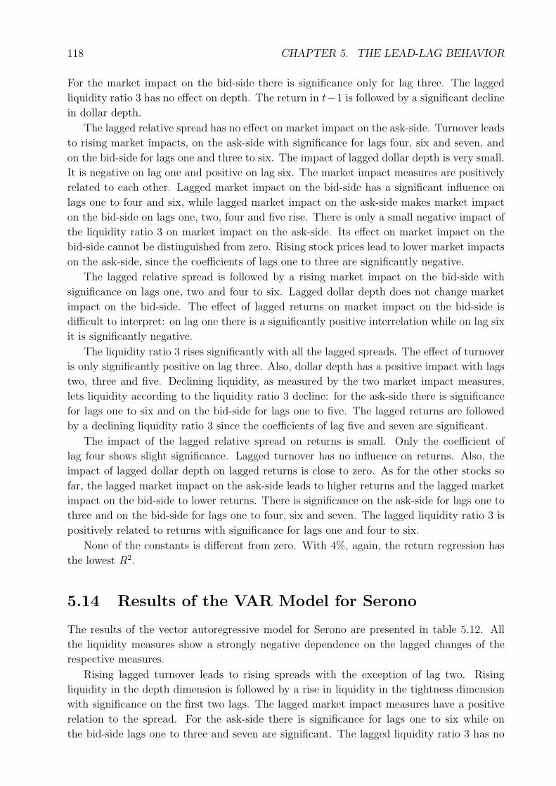
118 CHAPTER 5. THE LEAD-LAG BEHAVIOR
For the market impact on the bid-side there is significance only for lag three. The lagged
liquidity ratio 3 has no effect on depth. The return in t−1 is followed by a significant decline
in dollar depth.
The lagged relative spread has no effect on market impact on the ask-side. Turnover leads
to rising market impacts, on the ask-side with significance for lags four, six and seven, and
on the bid-side for lags one and three to six. The impact of lagged dollar depth is very small.
It is negative on lag one and positive on lag six. The market impact measures are positively
related to each other. Lagged market impact on the bid-side has a significant influence on
lags one to four and six, while lagged market impact on the ask-side makes market impact
on the bid-side on lags one, two, four and five rise. There is only a small negative impact of
the liquidity ratio 3 on market impact on the ask-side. Its effect on market impact on the
bid-side cannot be distinguished from zero. Rising stock prices lead to lower market impacts
on the ask-side, since the coefficients of lags one to three are significantly negative.
The lagged relative spread is followed by a rising market impact on the bid-side with
significance on lags one, two and four to six. Lagged dollar depth does not change market
impact on the bid-side. The effect of lagged returns on market impact on the bid-side is
difficult to interpret: on lag one there is a significantly positive interrelation while on lag six
it is significantly negative.
The liquidity ratio 3 rises significantly with all the lagged spreads. The effect of turnover
is only significantly positive on lag three. Also, dollar depth has a positive impact with lags
two, three and five. Declining liquidity, as measured by the two market impact measures,
lets liquidity according to the liquidity ratio 3 decline: for the ask-side there is significance
for lags one to six and on the bid-side for lags one to five. The lagged returns are followed
by a declining liquidity ratio 3 since the coefficients of lag five and seven are significant.
The impact of the lagged relative spread on returns is small. Only the coefficient of
lag four shows slight significance. Lagged turnover has no influence on returns. Also, the
impact of lagged dollar depth on lagged returns is close to zero. As for the other stocks so
far, the lagged market impact on the ask-side leads to higher returns and the lagged market
impact on the bid-side to lower returns. There is significance on the ask-side for lags one to
three and on the bid-side for lags one to four, six and seven. The lagged liquidity ratio 3 is
positively related to returns with significance for lags one and four to six.
None of the constants is different from zero. With 4%, again, the return regression has
the lowest R2.
5.14 Results of the VAR Model for Serono
The results of the vector autoregressive model for Serono are presented in table 5.12. All
the liquidity measures show a strongly negative dependence on the lagged changes of the
respective measures.
Rising lagged turnover leads to rising spreads with the exception of lag two. Rising
liquidity in the depth dimension is followed by a rise in liquidity in the tightness dimension
with significance on the first two lags. The lagged market impact measures have a positive
relation to the spread. For the ask-side there is significance for lags one to six while on
the bid-side lags one to three and seven are significant. The lagged liquidity ratio 3 has no
5.14. RESULTS OF THE VAR MODEL FOR SERONO 119
SrelMt Vt D$t MIA,V ∗t MIB,V ∗
t LR3 t rt
SrelMt−1 –0.70*** −4.08 · 107*** –1’828’409** –108.23*** –141.72 0.10*** –0.09**SrelMt−2 –0.59*** −4.06 · 107*** –1’273’651 –182.19*** –108.05 0.09*** 4.09 · 10−3
SrelMt−3 –0.47*** −3.14 · 107*** –1’411’740 –141.52*** 186.75 0.06*** –0.06SrelMt−4 –0.37*** −2.44 · 107*** –2’277’502* –110.12** 32.77 0.06*** –0.08SrelMt−5 –0.31*** −2.69 · 107*** –1’694’439 –133.47*** 125.83 0.05*** –0.09SrelMt−6 –0.20*** −1.30 · 107** –7’016 –142.26*** 42.29 0.02*** –0.13***SrelMt−7 –0.10*** –6’650’092 –188’542 –103.22*** 22.80 0.01** –0.16***
Vt−1 4.55 · 10−11*** –0.694*** 3.94 · 10−5 −1.38 · 10−8 3.89 · 10−7 2.21 · 10−11 −2.17 · 10−10**Vt−2 5.07 · 10−11 –0.512*** –0.002 −3.51 · 10−8 3.02 · 10−7 7.19 · 10−12 −1.58 · 10−10
Vt−3 8.42 · 10−11* –0.382*** –0.002 −1.28 · 10−7 1.60 · 10−7 1.40 · 10−11 8.97 · 10−11
Vt−4 9.68 · 10−11** –0.293*** –0.002 6.72 · 10−8 1.67 · 10−7 2.71 · 10−11 −1.24 · 10−10
Vt−5 8.37 · 10−11* –0.196*** –0.005* 7.65 · 10−8 1.99 · 10−7 3.12 · 10−11 3.74 · 10−11
Vt−6 9.87 · 10−11** –0.113*** –0.005* 1.02 · 10−7 2.94 · 10−8 3.64 · 10−11* −1.52 · 10−10
Vt−7 7.41 · 10−11** –0.072*** –0.004 2.50 · 10−8 −2.73 · 10−7 2.80 · 10−12 −1.01 · 10−10
D$t−1 −4.88 · 10−10** 0.833*** –0.673*** 4.94 · 10−7 −4.68 · 10−6*** −3.08 · 10−10*** 5.32 · 10−11
D$t−2 −6.07 · 10−10*** 0.635*** –0.545*** 6.63 · 10−7 −5.41 · 10−6*** −2.56 · 10−10** 1.23 · 10−9*D$t−3 −3.36 · 10−10 0.425*** –0.428*** 6.90 · 10−7 −1.65 · 10−6 −2.14 · 10−10* 2.20 · 10−9***D$t−4 −3.69 · 10−10 0.297*** –0.325*** 7.07 · 10−9 −1.65 · 10−6 −1.50 · 10−10 2.27 · 10−9***D$t−5 −3.15 · 10−11 0.327*** –0.230*** −1.41 · 10−7 −2.25 · 10−6 5.81 · 10−11 1.61 · 10−9**D$t−6 −2.18 · 10−10 0.167** –0.135*** −3.57 · 10−7 −2.62 · 10−6 3.51 · 10−11 1.05 · 10−9
D$t−7 8.79 · 10−11 0.250*** –0.075*** 1.60 · 10−7 −1.54 · 10−6 9.08 · 10−11 1.14 · 10−9*
MIA,V ∗t−1 1.99 · 10−5*** –3’001 –490 –0.448*** 0.146*** 9.49 · 10−6*** 4.25 · 10−5***
MIA,V ∗t−2 2.07 · 10−5*** –3’764 –967*** –0.336*** 0.141*** 1.17 · 10−5*** 4.84 · 10−5***
MIA,V ∗t−3 1.41 · 10−5** –1’896 –391 –0.225*** 0.095** 7.29 · 10−6*** 2.53 · 10−5
MIA,V ∗t−4 2.19 · 10−5*** –3’170 –166 –0.177*** 0.065 7.21 · 10−6*** 5.79 · 10−5***
MIA,V ∗t−5 1.34 · 10−5** –1’545 97 –0.144*** 0.016 6.40 · 10−6** 2.96 · 10−5*
MIA,V ∗t−6 2.20 · 10−5*** –1’377 339 –0.091*** 0.039 9.03 · 10−6*** 4.97 · 10−5***
MIA,V ∗t−7 1.22 · 10−6 580 216 –0.052*** 0.011 4.58 · 10−6** 4.67 · 10−5***
MIB,V ∗t−1 7.07 · 10−6*** 3’495*** –527*** 0.022*** –0.801*** 2.74 · 10−6*** −1.50 · 10−5***
MIB,V ∗t−2 5.90 · 10−6*** 2’803*** –553*** 0.009* –0.670*** 2.55 · 10−6*** −1.21 · 10−5**
MIB,V ∗t−3 3.96 · 10−6* 1’382* –549*** 0.010* –0.559*** 2.05 · 10−6** −1.18 · 10−5*
MIB,V ∗t−4 2.07 · 10−6 1’000 –555*** 0.008 –0.443*** 2.21 · 10−6** −1.62 · 10−5**
MIB,V ∗t−5 2.82 · 10−6 355 –517*** 0.004 –0.330*** 2.53 · 10−7 −1.10 · 10−5*
MIB,V ∗t−6 6.71 · 10−7 134 –379*** 0.005 –0.222*** 1.40 · 10−6 −1.10 · 10−5*
MIB,V ∗t−7 3.16 · 10−6** –762 –55 1.02 · 10−4 –0.115*** 1.81 · 10−6** −1.66 · 10−6
LR3 t−1 –0.001 8’771’788 583’031 8.89 88.30 –0.836*** 0.026LR3 t−2 0.009 –1’882’473 1’616’861 1.04 233.75 –0.696*** –0.195*LR3 t−3 0.037 −1.14 · 107 4’506’386* –42.88 607.90* –0.553*** –0.044LR3 t−4 0.056 –9’635’283 3’216’576 39.25 290.75 –0.453*** –0.028LR3 t−5 0.040 –8’032’515 656’227 122.61 147.18 –0.363*** 0.108LR3 t−6 0.010 –7’873’800 –809’519 44.90 –8.20 –0.240*** 0.130LR3 t−7 –0.011 –5’953’380 1’515’496 42.41 –123.94 –0.123*** 0.108
rt−1 0.003 –1’643’115 352’043 –35.13*** 44.60 –0.005** –0.089***rt−2 –0.007* –2’623’905* 268’110 –54.62*** 72.16** –0.002 –0.028**rt−3 –0.002 –567’919 302’115 –19.42* 47.01 –0.001 –0.020rt−4 –0.003 258’735 –670’605** –27.10** 70.23** –0.005*** 0.053***rt−5 0.003 1’323’578 67’616 –22.20** 53.91 0.001 0.018rt−6 0.008* –1’425’909 448’645 –5.96 50.45 0.003 0.018rt−7 0.000 –3’430’840** –417’005 –2.95 42.99 0.002 0.025**
C 0.00 –500.28 22.10 –0.01 0.03 0.00 0.00Adj.R2 0.33 0.37 0.33 0.20 0.40 0.42 0.02
Table 5.12: Vector autoregressive model of Serono with the first differences of six liquiditymeasures and returns including seven lags. */**/*** denotes significance on a level of10%/5%/1%.
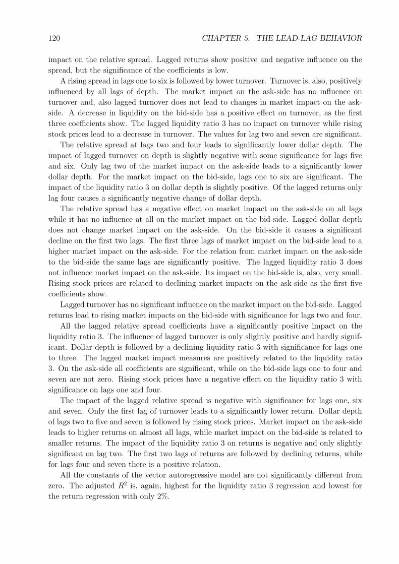
120 CHAPTER 5. THE LEAD-LAG BEHAVIOR
impact on the relative spread. Lagged returns show positive and negative influence on the
spread, but the significance of the coefficients is low.
A rising spread in lags one to six is followed by lower turnover. Turnover is, also, positively
influenced by all lags of depth. The market impact on the ask-side has no influence on
turnover and, also lagged turnover does not lead to changes in market impact on the ask-
side. A decrease in liquidity on the bid-side has a positive effect on turnover, as the first
three coefficients show. The lagged liquidity ratio 3 has no impact on turnover while rising
stock prices lead to a decrease in turnover. The values for lag two and seven are significant.
The relative spread at lags two and four leads to significantly lower dollar depth. The
impact of lagged turnover on depth is slightly negative with some significance for lags five
and six. Only lag two of the market impact on the ask-side leads to a significantly lower
dollar depth. For the market impact on the bid-side, lags one to six are significant. The
impact of the liquidity ratio 3 on dollar depth is slightly positive. Of the lagged returns only
lag four causes a significantly negative change of dollar depth.
The relative spread has a negative effect on market impact on the ask-side on all lags
while it has no influence at all on the market impact on the bid-side. Lagged dollar depth
does not change market impact on the ask-side. On the bid-side it causes a significant
decline on the first two lags. The first three lags of market impact on the bid-side lead to a
higher market impact on the ask-side. For the relation from market impact on the ask-side
to the bid-side the same lags are significantly positive. The lagged liquidity ratio 3 does
not influence market impact on the ask-side. Its impact on the bid-side is, also, very small.
Rising stock prices are related to declining market impacts on the ask-side as the first five
coefficients show.
Lagged turnover has no significant influence on the market impact on the bid-side. Lagged
returns lead to rising market impacts on the bid-side with significance for lags two and four.
All the lagged relative spread coefficients have a significantly positive impact on the
liquidity ratio 3. The influence of lagged turnover is only slightly positive and hardly signif-
icant. Dollar depth is followed by a declining liquidity ratio 3 with significance for lags one
to three. The lagged market impact measures are positively related to the liquidity ratio
3. On the ask-side all coefficients are significant, while on the bid-side lags one to four and
seven are not zero. Rising stock prices have a negative effect on the liquidity ratio 3 with
significance on lags one and four.
The impact of the lagged relative spread is negative with significance for lags one, six
and seven. Only the first lag of turnover leads to a significantly lower return. Dollar depth
of lags two to five and seven is followed by rising stock prices. Market impact on the ask-side
leads to higher returns on almost all lags, while market impact on the bid-side is related to
smaller returns. The impact of the liquidity ratio 3 on returns is negative and only slightly
significant on lag two. The first two lags of returns are followed by declining returns, while
for lags four and seven there is a positive relation.
All the constants of the vector autoregressive model are not significantly different from
zero. The adjusted R2 is, again, highest for the liquidity ratio 3 regression and lowest for
the return regression with only 2%.
5.15. RESULTS OF THE VAR MODEL FOR SURVEILLANCE 121
5.15 Results of the VAR Model for Surveillance
SrelMt Vt D$t MIA,V ∗t MIB,V ∗
t LR3 t rt
SrelMt−1 –0.55*** –9’961’203*** 1’376’086 38.68** –87.65 0.06*** –0.05**SrelMt−2 –0.46*** –5’484’717*** 2’460’961 38.14** –122.46** 0.08*** –0.10***SrelMt−3 –0.39*** –7’709’147*** –1’096’366 25.97 –364.31*** 0.08*** –0.06**SrelMt−4 –0.32*** –6’527’961*** –2’321’158 15.94 –368.19*** 0.05*** –0.05*SrelMt−5 –0.24*** –6’512’604*** –2’033’057 59.43*** –291.69*** 0.04*** –0.03SrelMt−6 –0.15*** –5’850’836*** –1’566’869 71.24*** –16.64 0.04*** –0.06**SrelMt−7 –0.08*** –2’326’076* –1’540’745 49.28*** –54.12 0.02*** –0.02
Vt−1 6.44 · 10−10*** –0.72*** –0.003 1.18 · 10−7 1.30 · 10−6*** 2.28 · 10−10*** 3.86 · 10−10*Vt−2 8.13 · 10−10*** –0.54*** –0.018 3.43 · 10−7* 7.24 · 10−7 1.98 · 10−10** −4.17 · 10−10
Vt−3 8.14 · 10−10*** –0.44*** –0.033 2.69 · 10−7 9.86 · 10−7 2.65 · 10−10*** −5.84 · 10−10**Vt−4 6.03 · 10−10*** –0.35*** –0.089 4.81 · 10−7** 1.30 · 10−6** 3.31 · 10−10*** −4.66 · 10−10
Vt−5 5.59 · 10−10*** –0.26*** 0.063 2.23 · 10−7 1.73 · 10−6*** 3.43 · 10−10*** −3.82 · 10−10
Vt−6 4.26 · 10−10*** –0.16*** 0.035 1.62 · 10−7 1.47 · 10−6** 1.84 · 10−10** −1.23 · 10−10
Vt−7 1.91 · 10−10* –0.07*** 0.005 −7.20 · 10−8 7.69 · 10−7 1.43 · 10−10** −2.67 · 10−12
D$t−1 1.33 · 10−11 0.003 –0.854*** 6.88 · 10−8* −1.34 · 10−9 4.81 · 10−13 1.11 · 10−11
D$t−2 7.38 · 10−12 0.001 –0.724*** 4.43 · 10−8 1.00 · 10−9 1.11 · 10−11 −4.20 · 10−12
D$t−3 −5.39 · 10−12 0.009* –0.595*** 6.06 · 10−8 2.73 · 10−8 1.39 · 10−11 −1.35 · 10−11
D$t−4 −6.89 · 10−12 0.018*** –0.469*** 5.73 · 10−8 −3.69 · 10−9 1.55 · 10−11 −3.54 · 10−11
D$t−5 2.84 · 10−12 0.011** –0.347*** 3.26 · 10−8 −1.04 · 10−8 9.14 · 10−12 −2.37 · 10−11
D$t−6 1.01 · 10−11 0.005 –0.226*** 1.65 · 10−8 −1.76 · 10−8 1.27 · 10−11 −1.47 · 10−11
D$t−7 2.95 · 10−12 0.001 –0.111*** 1.13 · 10−8 9.59 · 10−9 3.97 · 10−12 4.07 · 10−13
MIA,V ∗t−1 8.65 · 10−6 –3’656*** –1’683 –0.304*** 0.008 9.21 · 10−6 9.54 · 10−5***
MIA,V ∗t−2 4.57 · 10−6 –4’022*** –1’372 –0.215*** –0.034 2.18 · 10−5*** 1.07 · 10−4***
MIA,V ∗t−3 9.49 · 10−6 –3’491*** 22 –0.152*** 0.074* 2.07 · 10−5*** 1.11 · 10−4***
MIA,V ∗t−4 2.85 · 10−5*** –4’316*** –107 –0.118*** 0.067 1.07 · 10−5 1.30 · 10−4***
MIA,V ∗t−5 2.26 · 10−5** –1’462 5’784 –0.114*** 0.018 −4.06 · 10−6 5.54 · 10−5***
MIA,V ∗t−6 9.69 · 10−6 –2’442** –775 –0.087*** –0.061 8.68 · 10−6 3.85 · 10−5**
MIA,V ∗t−7 1.55 · 10−5 –1’642 –798 –0.037*** 0.042 −5.41 · 10−6 2.81 · 10−5
MIB,V ∗t−1 1.52 · 10−5*** 523 –450 –0.002 –0.572*** 5.90 · 10−6*** −8.50 · 10−7
MIB,V ∗t−2 6.02 · 10−6* 931** –511 0.005 –0.178*** 3.19 · 10−6 −1.40 · 10−5**
MIB,V ∗t−3 2.43 · 10−5*** 991*** 134 0.005 –0.137*** 4.07 · 10−6* −2.70 · 10−5***
MIB,V ∗t−4 2.14 · 10−5*** 991*** 398 0.012*** –0.008 1.53 · 10−6 −4.95 · 10−5***
MIB,V ∗t−5 1.91 · 10−5*** 1’013*** 208 –0.002 0.042*** −2.01 · 10−6 −4.30 · 10−5***
MIB,V ∗t−6 6.22 · 10−6* 157 298 –0.007 –0.191*** 7.22 · 10−7 −1.88 · 10−5***
MIB,V ∗t−7 3.68 · 10−6 –372 219 –0.002 –0.210*** 1.39 · 10−6 −5.69 · 10−6
LR3 t−1 0.018 –1’698’619 –2’829’382 –60.93** –147.47* –0.841*** 0.076**LR3 t−2 0.023 36’652 –2’369’765 –46.32 –201.77* –0.694*** 0.081*LR3 t−3 –0.012 –3’489’346 –2’154’874 –55.56 –295.78** –0.549*** 0.091*LR3 t−4 0.006 –7’355’803** –5’531’381 –50.43 –221.77* –0.433*** 0.035LR3 t−5 –0.016 –7’102’558** –5’925’316 –21.62 –262.08** –0.333*** –0.028LR3 t−6 –0.060** –7’904’589*** –4’461’456 18.23 –194.32* –0.230*** –0.054LR3 t−7 –0.018 –6’307’993*** –4’184’608 20.11 –178.57** –0.120*** 0.014
rt−1 –0.020*** 1’155’684 –488’186 –3.35 51.89* 0.001 –0.215***rt−2 0.002 1’181’806 469’039 –28.22*** 125.66*** –0.002 –0.109***rt−3 0.007 –800’279 937’074 –13.27 145.11*** 0.008* –0.082***rt−4 0.009 –1’957’724** 799’585 1.50 35.68 –0.005 –0.034***rt−5 –0.007 –1’865’891** 2’788’393 7.85 8.20 –0.005 –0.024*rt−6 –0.006 –1’816’902** –95’374 –9.84 18.20 0.012 0.005rt−7 –0.004 –1’696’025** 350’726 –18.77** 3.01 –0.007 0.031**
C 0.00 42.13 65.52 0.00 0.00 0.00 0.00Adj.R2 0.25 0.36 0.42 0.10 0.31 0.42 0.07
Table 5.13: Vector autoregressive model of Surveillance with the first differences of sixliquidity measures and returns including seven lags. */**/*** denotes significance on a levelof 10%/5%/1%.
Table 5.13 presents the results of the vector autoregressive model for Surveillance. Almost
all the lagged changes in liquidity measures are significantly negatively related to the changes
of the respective liquidity measures in time t. Only the coefficient of market impact on the
bid-side on lag four is not significantly different from zero.
122 CHAPTER 5. THE LEAD-LAG BEHAVIOR
Lagged turnover leads to a rising spread with significance on all lags. Lagged dollar depth
has no impact on the relative spread. The market impact on the ask-side has, with its lags
four and five, a positive effect on the relative spread. Also the market impact on the bid-side
has a significant influence on the relative spread. It is significant for lags one to six. The
liquidity ratio 3 on lag six is followed by a declining relative spread. The return in time t−1
has a positive relation to liquidity in the tightness dimension.
All the lagged relative spreads decrease turnover. Dollar depth is, with its lags three
to five, positively related to turnover. This is the only influence of dollar depth on the
other variables of the vector autoregressive model, with the exception of a slightly positive
impact on the market impact on the ask-side. The market impact on the ask-side leads to
significantly lower turnover on lags one to four and six. On the other hand, market impact
on the bid-side leads to significantly higher turnover with lags two to five. The lags four to
seven of the liquidity ratio 3 decrease turnover. Rising stock prices of lags four to seven are
followed by declining turnover.
What is new for Surveillance with respect to the previous stocks is that dollar depth
depends only on lagged dollar depth itself. The other five liquidity measures and returns do
not have any significant impact.
A rising lagged spread has a positive influence on market impact on the ask-side on lags
one, two and five to seven. Also, turnover on lags two and four leads to a higher market
impact on the ask-side. Only lag four of the market impact on the bid-side has a significant
influence on market impact on the ask-side. The liquidity ratio 3 has a significantly negative
impact with lag one on market impact on the ask-side. Also, rising stock prices lead to
smaller market impacts on the ask-side, with significance for lags two and seven.
The rising relative spread reduces the market impact on the bid-side, significantly on lags
two to five. Rising turnover leads to a rising market impact on the bid-side, with significance
for lags one and four to six. There is only a small impact of lagged market impact on the
ask-side with respect to market impact on the bid-side. All lags of the liquidity ratio 3 are
followed by a declining market impact on the bid-side. A rising stock price leads to higher
market impacts on the bid-side, with significance for lags one to three.
All the lagged relative spreads are related to a rising liquidity ratio 3. All the lagged
turnovers have the same impact. The market impact measures lead to a higher liquidity
ratio 3. For the ask-side there is significance for lags two and three and for the bid-side for
lags one and three. The lagged returns only have a slightly positive impact on lag three.
Return reacts negatively on changes in the lagged relative spread with significance for
lags one to four and six. Turnover on lag one is related to rising returns, while turnover on
lag three is followed by declining returns. The market impact on the ask-side leads, with lags
one to six, to larger returns. The lags two to six of market impact on the bid-side are related
to smaller returns. The liquidity ratio 3 is positively related to returns with significance for
lags one to three. Return depends negatively on the lagged returns for the first five lags.
The interrelation of lag seven and return in time t is significantly positive.
All the constants of the model are close to zero. The adjusted R2-values are in the range
of the previous stocks.
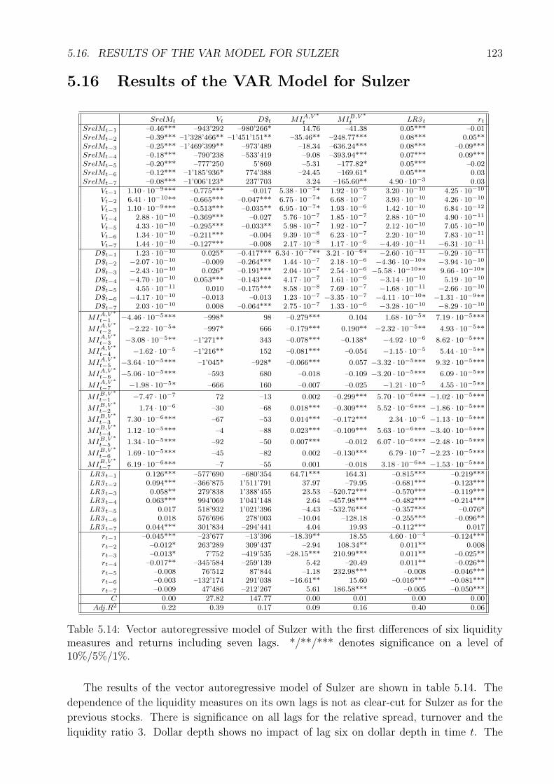
5.16. RESULTS OF THE VAR MODEL FOR SULZER 123
5.16 Results of the VAR Model for Sulzer
SrelMt Vt D$t MIA,V ∗t MIB,V ∗
t LR3 t rt
SrelMt−1 –0.46*** –943’292 –980’266* 14.76 –41.38 0.05*** –0.01SrelMt−2 –0.39*** –1’328’466** –1’451’151** –35.46** –248.77*** 0.08*** 0.05**SrelMt−3 –0.25*** –1’469’399** –973’489 –18.34 –636.24*** 0.08*** –0.09***SrelMt−4 –0.18*** –790’238 –533’419 –9.08 –393.94*** 0.07*** 0.09***SrelMt−5 –0.20*** –777’250 5’869 –5.31 –177.82* 0.05*** –0.02SrelMt−6 –0.12*** –1’185’936* 774’388 –24.45 –169.61* 0.05*** 0.03SrelMt−7 –0.08*** –1’006’123* 237’703 3.24 –165.60** 4.90 · 10−3 0.03
Vt−1 1.10 · 10−9*** –0.775*** –0.017 5.38 · 10−7* 1.92 · 10−6 3.20 · 10−10 4.25 · 10−10
Vt−2 6.41 · 10−10** –0.665*** –0.047*** 6.75 · 10−7* 6.68 · 10−7 3.93 · 10−10 4.26 · 10−10
Vt−3 1.10 · 10−9*** –0.513*** –0.035** 6.95 · 10−7* 1.93 · 10−6 1.42 · 10−10 6.84 · 10−12
Vt−4 2.88 · 10−10 –0.369*** –0.027 5.76 · 10−7 1.85 · 10−7 2.88 · 10−10 4.90 · 10−11
Vt−5 4.33 · 10−10 –0.295*** –0.033** 5.98 · 10−7 1.92 · 10−7 2.12 · 10−10 7.05 · 10−10
Vt−6 1.34 · 10−10 –0.211*** –0.004 9.39 · 10−8 6.23 · 10−7 2.20 · 10−10 7.83 · 10−11
Vt−7 1.44 · 10−10 –0.127*** –0.008 2.17 · 10−8 1.17 · 10−6 −4.49 · 10−11 −6.31 · 10−11
D$t−1 1.23 · 10−10 0.025* –0.417*** 6.34 · 10−7** 3.21 · 10−6* −2.60 · 10−11 −9.29 · 10−11
D$t−2 −2.07 · 10−10 –0.009 –0.264*** 1.44 · 10−7 2.18 · 10−6 −4.36 · 10−10* −3.94 · 10−10
D$t−3 −2.43 · 10−10 0.026* –0.191*** 2.04 · 10−7 2.54 · 10−6 −5.58 · 10−10** 9.66 · 10−10*D$t−4 −4.70 · 10−10 0.053*** –0.143*** 4.17 · 10−7 1.61 · 10−6 −3.14 · 10−10 5.19 · 10−10
D$t−5 4.55 · 10−11 0.010 –0.175*** 8.58 · 10−8 7.69 · 10−7 −1.68 · 10−11 −2.66 · 10−10
D$t−6 −4.17 · 10−10 –0.013 –0.013 1.23 · 10−7 −3.35 · 10−7 −4.11 · 10−10* −1.31 · 10−9**D$t−7 2.03 · 10−10 0.008 –0.064*** 2.75 · 10−7 1.33 · 10−6 −3.28 · 10−10 −8.29 · 10−10
MIA,V ∗t−1 −4.46 · 10−5*** –998* 98 –0.279*** 0.104 1.68 · 10−5* 7.19 · 10−5***
MIA,V ∗t−2 −2.22 · 10−5* –997* 666 –0.179*** 0.190** −2.32 · 10−5** 4.93 · 10−5**
MIA,V ∗t−3 −3.08 · 10−5** –1’271** 343 –0.078*** –0.138* −4.92 · 10−6 8.62 · 10−5***
MIA,V ∗t−4 −1.62 · 10−5 –1’216** 152 –0.081*** –0.054 −1.15 · 10−5 5.44 · 10−5**
MIA,V ∗t−5 −3.64 · 10−5*** –1’045* –928* –0.066*** 0.057 −3.32 · 10−5*** 9.32 · 10−5***
MIA,V ∗t−6 −5.06 · 10−5*** –593 680 –0.018 –0.109 −3.20 · 10−5*** 6.09 · 10−5**
MIA,V ∗t−7 −1.98 · 10−5* –666 160 –0.007 –0.025 −1.21 · 10−5 4.55 · 10−5**
MIB,V ∗t−1 −7.47 · 10−7 72 –13 0.002 –0.299*** 5.70 · 10−6*** −1.02 · 10−5***
MIB,V ∗t−2 1.74 · 10−6 –30 –68 0.018*** –0.309*** 5.52 · 10−6*** −1.86 · 10−5***
MIB,V ∗t−3 7.30 · 10−6*** –67 –53 0.014*** –0.172*** 2.34 · 10−6 −1.13 · 10−5***
MIB,V ∗t−4 1.12 · 10−5*** –4 –88 0.023*** –0.109*** 5.63 · 10−6*** −3.40 · 10−5***
MIB,V ∗t−5 1.34 · 10−5*** –92 –50 0.007*** –0.012 6.07 · 10−6*** −2.48 · 10−5***
MIB,V ∗t−6 1.69 · 10−5*** –45 –82 0.002 –0.130*** 6.79 · 10−7 −2.23 · 10−5***
MIB,V ∗t−7 6.19 · 10−6*** –7 –55 0.001 –0.018 3.18 · 10−6** −1.53 · 10−5***
LR3 t−1 0.126*** –577’690 –680’354 64.71*** 164.31 –0.815*** –0.219***LR3 t−2 0.094*** –366’875 1’511’791 37.97 –79.95 –0.681*** –0.123***LR3 t−3 0.058** 279’838 1’388’455 23.53 –520.72*** –0.570*** –0.119***LR3 t−4 0.063*** 994’069 1’041’148 2.64 –457.98*** –0.482*** –0.214***LR3 t−5 0.017 518’932 1’021’396 –4.43 –532.76*** –0.357*** –0.076*LR3 t−6 0.018 576’696 278’003 –10.04 –128.18 –0.255*** –0.096**LR3 t−7 0.044*** 301’834 –294’441 4.04 19.93 –0.112*** 0.017
rt−1 –0.045*** –23’677 –13’396 –18.39** 18.55 4.60 · 10−4 –0.124***rt−2 –0.012* 263’289 309’437 –2.94 108.34** 0.011** 0.008rt−3 –0.013* 7’752 –419’535 –28.15*** 210.99*** 0.011** –0.025**rt−4 –0.017** –345’584 –259’139 5.42 –20.49 0.011** –0.026**rt−5 –0.008 76’512 87’844 –1.18 232.98*** –0.008 –0.046***rt−6 –0.003 –132’174 291’038 –16.61** 15.60 –0.016*** –0.081***rt−7 –0.009 47’486 –212’267 5.61 186.58*** –0.005 –0.050***
C 0.00 27.82 147.77 0.00 0.01 0.00 0.00Adj.R2 0.22 0.39 0.17 0.09 0.16 0.40 0.06
Table 5.14: Vector autoregressive model of Sulzer with the first differences of six liquiditymeasures and returns including seven lags. */**/*** denotes significance on a level of10%/5%/1%.
The results of the vector autoregressive model of Sulzer are shown in table 5.14. The
dependence of the liquidity measures on its own lags is not as clear-cut for Sulzer as for the
previous stocks. There is significance on all lags for the relative spread, turnover and the
liquidity ratio 3. Dollar depth shows no impact of lag six on dollar depth in time t. The
124 CHAPTER 5. THE LEAD-LAG BEHAVIOR
lags six and seven of market impact on the ask-side do not influence market impact on the
ask-side in time t. Market impact on the bid-side on lags five and seven do not lead to any
significant changes of the market impact on the bid-side.
The lags one to three of turnover lead to a significantly higher relative spread, while dollar
depth has no significant impact on the spread. Market impact on the ask-side is related to
a declining spread, with significance on almost all lags; this in contrast to some of the other
stocks. Market impact on the bid-side leads to a significantly higher spread for lags three to
seven. The liquidity ratio 3 has a significantly positive impact on the relative spread on lags
one to four and seven. Rising stock prices tend to decrease the spread, as the coefficients of
the first four lags show.
The lagged relative spread reduces turnover significantly on lags two, three, six and seven.
Increasing dollar depth leads to higher turnover on lags one, three and four. The market
impact on the ask-side reduces turnover with its lags one to five, while the market impact on
the bid-side does not change turnover significantly. In the other direction, lagged turnover
has no impact on market impact on the bid-side. The lagged liquidity ratio 3 and the lagged
returns have no significant impact on turnover and lagged turnover does not change either
the liquidity ratio 3 or returns.
A rising spread in lags one and two leads to a significantly declining dollar depth.
Turnover has a significantly negative impact on dollar depth on lags two, three and five.
The influence of the market impact on dollar depth is almost not distinguishable from zero.
The lagged liquidity ratio 3 and lagged returns do not have any significant impact on dollar
depth.
Only the second lag of the relative spread makes the market impact on the ask-side
decrease significantly. Turnover leads to a higher market impact on the ask-side, as slightly
significant lags one to three show. A rise in dollar depth is followed by a rise in market
impact on the ask-side. Rising market impact on the bid-side is positively related to market
impact on the ask-side on lags two to five. The first lag of the liquidity ratio 3 has a positive
effect on market impact on the ask-side. The lagged returns have a negative influence on
the market impact on the ask-side on lags one, three and six.
The lagged relative spread leads to a decrease in market impact on the bid-side with
significance at almost all lags. Only the first lag of dollar depth is slightly positively related
to market impact on the bid-side. Market impact on the ask-side leads with lag two to a
significantly higher market impact on the bid-side. In contrast to this, lag three is signifi-
cantly negative on the 10% level. The liquidity ratio 3 leads to a lower market impact on
the bid-side since lags three to five are significantly different from zero. Rising stock prices
are followed by a larger market impact on the bid-side with significance for lags two, three,
five and seven.
The liquidity ratio 3 is positively affected by the relative spread on lags one to six. Dollar
depth has a significantly negative effect on the liquidity ratio 3 on lags two, three and six.
The market impact on the ask-side leads to a significantly lower liquidity ratio 3 on lags two,
five and six, while on lag one there is a slightly negative significance. The market impact
on the bid-side affects the liquidity ratio 3 positively on lags one, two, four, five and seven.
The returns on lag two to four make the liquidity ratio 3 rise while the lag six decreases it.
The impact of the relative spread on returns is ambiguous: on lag three it is significantly
5.17. RESULTS OF THE VAR MODEL FOR SYNGENTA 125
negative while on lags two and four it is positive. Dollar depth also shows positive and
negative influence on returns. Positive significance is found for lag three and a negative one
for lag six. All the lagged market impacts on the ask-side lead to higher returns, while all
the market impacts on the bid-side are related to lower returns. The liquidity ratio 3 leads
on lags one to six to lower returns. The return depends on its own lags negatively. There is
significance for lags one and three to seven.
None of the constants of the model is significantly different from zero. The adjusted R2
is, with 6% for the returns regression, so far relatively high. The other R2-values are in line
with the ones of the other stocks.
5.17 Results of the VAR Model for Syngenta
The results of the vector autoregressive model for Syngenta are presented in table 5.15.
Again, we have the clear negative dependence of the liquidity measures on its own lagged
realizations. The coefficients are all highly significant.
The relative spread is strongly positively influenced by turnover up to lag six. Lagged
dollar depth does not influence the relative spread significantly. The lagged spread shows
only a very small impact on dollar depth. Market impact on the ask-side leads on lags one
to three and six to a significantly higher spread. The seventh lag is negatively related to
the relative spread. Lags one to four of market impact on the bid-side increase the spread.
The impact of the lagged liquidity ratio 3 on the relative spread is only slightly significant
on lag seven. The coefficient is negative. Lagged returns do not influence the spread of the
Syngenta stock at all.
All the lags of the relative spread have a highly significant negative impact on turnover.
Dollar depth is positively related to turnover on the first three lags. The market impact
measures lead to decreasing turnover. On the ask-side the first lag is significant while on
the bid-side the first two coefficients are significantly different from zero. The impact of the
liquidity ratio 3 on turnover is negative but there is only significance at the 10% level. The
lagged returns have no impact on turnover at all.
Dollar depth is neither changed by lagged turnover nor by the market impact on the
ask-side. The market impact on the bid-side has a significantly negative influence on lags
one, two and five. The lagged liquidity ratio 3 and the lagged returns do not change dollar
depth significantly.
The relative spread on lags five and six decreases market impact on the ask-side. The
impact of lagged turnover on the market impact on the ask-side is only slightly significant on
lag four. Also, lagged dollar depth has only a very small positive influence on market impact
on the ask-side. The first four lags of market impact on the bid-side lead to a significant
rise in market impact on the ask-side. The liquidity ratio 3 has no influence on the market
impact measures. Increasing stock prices lead to a decrease in market impact on the ask-side
with significance on almost all lags.
Decreasing liquidity in the tightness dimension increases the market impact on the bid-
side with significance for lags one to five. For lag seven there is a slightly negative effect. The
influence of lagged turnover on market impact on the bid-side is negative but only slightly
significant. Dollar depth does not change market impact on the bid-side at all. The lagged
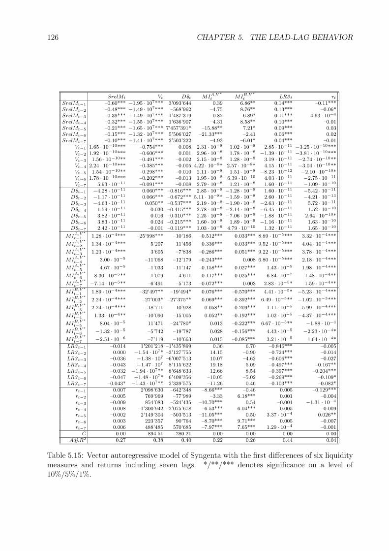
126 CHAPTER 5. THE LEAD-LAG BEHAVIOR
SrelMt Vt D$t MIA,V ∗t MIB,V ∗
t LR3 t rt
SrelMt−1 –0.60*** −1.95 · 107*** 3’093’644 0.39 6.86** 0.14*** –0.11***SrelMt−2 –0.48*** −1.49 · 107*** –568’962 –4.75 8.76** 0.13*** –0.06*SrelMt−3 –0.39*** −1.49 · 107*** –1’487’319 –0.82 6.89* 0.11*** 4.63 · 10−4
SrelMt−4 –0.32*** −1.55 · 107*** 1’636’907 –4.31 8.58** 0.10*** –0.01SrelMt−5 –0.21*** −1.65 · 107*** 7’457’391* –15.88** 7.21* 0.09*** 0.03SrelMt−6 –0.15*** −1.32 · 107*** 5’506’027 –21.33*** –2.41 0.06*** 0.02SrelMt−7 –0.10*** −1.41 · 107*** 2’503’222 –4.93 –6.01* 0.04*** –0.01
Vt−1 1.65 · 10−10*** –0.754*** 0.008 2.31 · 10−8 1.02 · 10−8 2.85 · 10−11 −3.25 · 10−10***Vt−2 1.92 · 10−10*** –0.606*** 0.001 2.96 · 10−8 1.78 · 10−8 −1.39 · 10−11 −3.81 · 10−10***Vt−3 1.56 · 10−10** –0.491*** –0.002 2.15 · 10−8 1.28 · 10−8 3.19 · 10−11 −2.74 · 10−10**Vt−4 2.24 · 10−10*** –0.385*** –0.005 4.22 · 10−8* 2.57 · 10−8* 4.15 · 10−11 −3.04 · 10−10**Vt−5 1.54 · 10−10** –0.298*** –0.010 2.11 · 10−8 1.51 · 10−8 −8.23 · 10−12 −2.10 · 10−10*Vt−6 1.78 · 10−10*** –0.202*** –0.013 1.95 · 10−8 6.39 · 10−10 4.03 · 10−11 −2.75 · 10−11
Vt−7 5.93 · 10−11 –0.091*** –0.008 2.79 · 10−8 1.21 · 10−8 1.60 · 10−11 −1.09 · 10−10
D$t−1 −4.28 · 10−11 0.060*** –0.816*** 2.85 · 10−8 −1.28 · 10−8 1.60 · 10−11 −5.42 · 10−11
D$t−2 −1.17 · 10−11 0.066*** –0.672*** 5.11 · 10−8* −1.59 · 10−8 2.60 · 10−11 −4.21 · 10−13
D$t−3 −4.63 · 10−11 0.050** –0.537*** 2.19 · 10−8 −1.90 · 10−8 −2.63 · 10−11 5.72 · 10−11
D$t−4 1.59 · 10−11 0.030 –0.415*** 2.78 · 10−8 −2.14 · 10−8 −6.45 · 10−11 1.52 · 10−10
D$t−5 3.82 · 10−11 0.016 –0.310*** 2.25 · 10−8 −7.06 · 10−9 −1.88 · 10−11 2.64 · 10−10*D$t−6 3.83 · 10−11 0.024 –0.215*** 1.60 · 10−8 1.89 · 10−9 −1.16 · 10−11 1.63 · 10−10
D$t−7 2.42 · 10−11 –0.001 –0.119*** 1.03 · 10−9 4.79 · 10−10 1.32 · 10−11 1.65 · 10−10
MIA,V ∗t−1 1.28 · 10−4*** –25’998*** –10’186 –0.512*** 0.033*** 8.89 · 10−5*** 3.32 · 10−4***
MIA,V ∗t−2 1.34 · 10−4*** –5’207 –11’456 –0.336*** 0.033*** 9.52 · 10−5*** 4.04 · 10−4***
MIA,V ∗t−3 1.23 · 10−4*** 3’605 –7’838 –0.286*** 0.051*** 9.22 · 10−5*** 3.78 · 10−4***
MIA,V ∗t−4 3.00 · 10−5 –11’068 –12’179 –0.243*** 0.008 6.80 · 10−5*** 2.18 · 10−4***
MIA,V ∗t−5 4.67 · 10−5 –1’033 –11’147 –0.158*** 0.027*** 1.43 · 10−5 1.98 · 10−4***
MIA,V ∗t−6 8.30 · 10−5** 1’079 –4’611 –0.117*** 0.025*** 6.84 · 10−7 1.48 · 10−4**
MIA,V ∗t−7 −7.14 · 10−5** –6’491 –5’173 –0.072*** 0.003 2.83 · 10−5* 1.59 · 10−4**
MIB,V ∗t−1 1.89 · 10−4*** –32’497** –19’494* 0.076*** –0.570*** 4.41 · 10−5* −5.23 · 10−4***
MIB,V ∗t−2 2.24 · 10−4*** –27’003* –27’375** 0.069*** –0.392*** 6.49 · 10−5** −1.02 · 10−3***
MIB,V ∗t−3 2.24 · 10−4*** –18’711 –10’928 0.058** –0.209*** 1.11 · 10−5 −5.99 · 10−4***
MIB,V ∗t−4 1.33 · 10−4** –10’090 –15’005 0.052** –0.192*** 1.02 · 10−5 −4.37 · 10−4***
MIB,V ∗t−5 8.04 · 10−5 11’471 –24’780* 0.013 –0.222*** 6.67 · 10−5** −1.88 · 10−4
MIB,V ∗t−6 −1.32 · 10−5 –5’742 –19’787 0.028 –0.156*** 4.43 · 10−5 −2.23 · 10−4*
MIB,V ∗t−7 −2.51 · 10−6 –7’119 –10’663 0.015 –0.085*** 3.21 · 10−5 1.64 · 10−4*
LR3 t−1 –0.014 1’201’218 –1’435’899 0.36 6.70 –0.846*** –0.005LR3 t−2 0.000 −1.54 · 107* –3’127’755 14.15 –0.90 –0.724*** –0.014LR3 t−3 –0.036 −1.38 · 107 –6’007’513 10.07 –4.62 –0.606*** –0.027LR3 t−4 –0.043 −1.47 · 107 8’115’622 19.18 5.09 –0.497*** –0.167**LR3 t−5 –0.032 −1.94 · 107** 8’648’633 12.66 8.54 –0.397*** –0.204***LR3 t−6 –0.047 −1.48 · 107* 6’409’356 –10.05 –5.02 –0.269*** –0.109*LR3 t−7 –0.043* −1.43 · 107** 2’339’575 –11.26 0.46 –0.103*** –0.082*
rt−1 0.007 2’098’630 –642’348 –8.66*** –0.46 0.005 –0.129***rt−2 –0.005 769’969 –77’989 –3.33 6.18*** 0.001 –0.004rt−3 –0.009 854’083 –524’435 –10.70*** 0.54 –0.001 −1.31 · 10−4
rt−4 0.008 –1’300’942 –2’075’678 –6.53*** 6.04*** 0.005 –0.009rt−5 –0.002 2’149’304 –503’513 –11.05*** 0.50 3.37 · 10−4 0.026**rt−6 0.003 223’357 90’764 –8.70*** 9.71*** 0.005 –0.007rt−7 0.006 488’485 570’685 –7.97*** 7.65*** 1.29 · 10−4 –0.001
C 0.00 894.51 –280.21 0.00 0.00 0.00 0.00Adj.R2 0.27 0.38 0.40 0.22 0.26 0.44 0.04
Table 5.15: Vector autoregressive model of Syngenta with the first differences of six liquiditymeasures and returns including seven lags. */**/*** denotes significance on a level of10%/5%/1%.
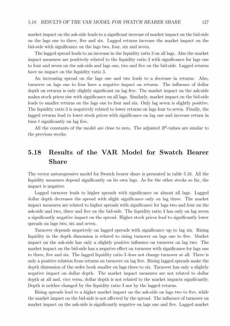
5.18. RESULTS OF THE VAR MODEL FOR SWATCH BEARER SHARE 127
market impact on the ask-side leads to a significant increase of market impact on the bid-side
on the lags one to three, five and six. Lagged returns increase the market impact on the
bid-side with significance on the lags two, four, six and seven.
The lagged spread leads to an increase in the liquidity ratio 3 on all lags. Also the market
impact measures are positively related to the liquidity ratio 3 with significance for lags one
to four and seven on the ask-side and lags one, two and five on the bid-side. Lagged returns
have no impact on the liquidity ratio 3.
An increasing spread on the lags one and two leads to a decrease in returns. Also,
turnover on lags one to four have a negative impact on returns. The influence of dollar
depth on returns is only slightly significant on lag five. The market impact on the ask-side
makes stock prices rise with significance on all lags. Similarly, market impact on the bid-side
leads to smaller returns on the lags one to four and six. Only lag seven is slightly positive.
The liquidity ratio 3 is negatively related to lower returns on lags four to seven. Finally, the
lagged returns lead to lower stock prices with significance on lag one and increase return in
time t significantly on lag five.
All the constants of the model are close to zero. The adjusted R2-values are similar to
the previous stocks.
5.18 Results of the VAR Model for Swatch Bearer
Share
The vector autoregressive model for Swatch bearer share is presented in table 5.16. All the
liquidity measures depend significantly on its own lags. As for the other stocks so far, the
impact is negative.
Lagged turnover leads to higher spreads with significance on almost all lags. Lagged
dollar depth decreases the spread with slight significance only on lag three. The market
impact measures are related to higher spreads with significance for lags two and four on the
ask-side and two, three and five on the bid-side. The liquidity ratio 3 has only on lag seven
a significantly negative impact on the spread. Higher stock prices lead to significantly lower
spreads on lags two, six and seven.
Turnover depends negatively on lagged spreads with significance up to lag six. Rising
liquidity in the depth dimension is related to rising turnover on lags one to five. Market
impact on the ask-side has only a slightly positive influence on turnover on lag two. The
market impact on the bid-side has a negative effect on turnover with significance for lags one
to three, five and six. The lagged liquidity ratio 3 does not change turnover at all. There is
only a positive relation from returns on turnover on lag five. Rising lagged spreads make the
depth dimension of the order book smaller on lags three to six. Turnover has only a slightly
negative impact on dollar depth. The market impact measures are not related to dollar
depth at all and, vice versa, dollar depth is not related to the market impacts significantly.
Depth is neither changed by the liquidity ratio 3 nor by the lagged returns.
Rising spreads lead to a higher market impact on the ask-side on lags two to five, while
the market impact on the bid-side is not affected by the spread. The influence of turnover on
market impact on the ask-side is significantly negative on lags one and five. Lagged market
128 CHAPTER 5. THE LEAD-LAG BEHAVIOR
SrelMt Vt D$t MIA,V ∗t MIB,V ∗
t LR3 t rt
SrelMt−1 –0.65*** −1.22 · 107*** –1’234’742 3.44 –0.43 0.13*** –0.04*SrelMt−2 –0.50*** −1.08 · 107*** –1’527’133 15.66** 5.53 0.15*** –0.03SrelMt−3 –0.40*** –5’816’168*** –1’882’606* 16.48** 2.36 0.13*** –0.09***SrelMt−4 –0.33*** –7’064’369*** –2’870’308*** 22.01*** 4.47 0.10*** –0.02SrelMt−5 –0.27*** –5’557’226*** –2’434’233** 14.19* –2.92 0.07*** –0.09***SrelMt−6 –0.17*** –3’312’377* –1’961’828** 6.80 4.68 0.06*** –0.05*SrelMt−7 –0.11*** –986’704 –889’287 7.30 1.31 0.03*** –0.03
Vt−1 5.01 · 10−10*** –0.792*** −5.84 · 10−5 −1.21 · 10−7*** 4.63 · 10−8 −2.01 · 10−11 3.48 · 10−11
Vt−2 5.57 · 10−10*** –0.626*** –0.013* −4.90 · 10−8 9.26 · 10−8** −7.40 · 10−11 −1.11 · 10−10
Vt−3 4.35 · 10−10*** –0.495*** –0.013 −6.66 · 10−8 3.91 · 10−8 −8.45 · 10−11 −3.16 · 10−10
Vt−4 2.11 · 10−10 –0.380*** –0.008 −9.81 · 10−8 7.52 · 10−9 −1.04 · 10−10 −5.58 · 10−10*Vt−5 2.75 · 10−10* –0.287*** –0.003 −1.11 · 10−7* 1.15 · 10−8 −1.14 · 10−10 −3.15 · 10−10
Vt−6 2.93 · 10−10** –0.180*** –0.007 2.47 · 10−9 2.42 · 10−8 −4.29 · 10−11 −4.02 · 10−11
Vt−7 3.35 · 10−10*** –0.086*** –0.001 5.63 · 10−8 −6.84 · 10−9 5.17 · 10−11 −1.83 · 10−11
D$t−1 −1.51 · 10−11 0.234*** –0.464*** 1.09 · 10−7 3.10 · 10−8 −9.54 · 10−11 3.52 · 10−10
D$t−2 −2.41 · 10−10 0.352*** –0.396*** 4.09 · 10−9 5.00 · 10−8 −2.77 · 10−12 −2.78 · 10−10
D$t−3 −4.10 · 10−10* 0.242*** –0.267*** 1.71 · 10−7 3.96 · 10−8 −1.55 · 10−10 −5.02 · 10−11
D$t−4 −6.48 · 10−11 0.184*** –0.157*** −2.74 · 10−8 2.77 · 10−8 −9.36 · 10−11 1.30 · 10−10
D$t−5 −2.53 · 10−11 0.143*** –0.161*** 3.31 · 10−8 2.51 · 10−8 5.36 · 10−11 4.97 · 10−11
D$t−6 −2.47 · 10−10 0.047 –0.137*** 7.67 · 10−8 7.59 · 10−8 1.74 · 10−11 5.00 · 10−10
D$t−7 −1.45 · 10−11 0.028 –0.133*** 1.31 · 10−7 −3.29 · 10−8 2.27 · 10−10* −9.54 · 10−11
MIA,V ∗t−1 4.83 · 10−5 758 –563 –0.394*** 0.011 2.27 · 10−5 2.59 · 10−4***
MIA,V ∗t−2 1.24 · 10−4*** 7’559* –2’196 –0.239*** 0.015 1.27 · 10−5 2.77 · 10−4***
MIA,V ∗t−3 1.78 · 10−5 –2’238 –1’292 –0.220*** 0.013 5.25 · 10−6 2.14 · 10−4***
MIA,V ∗t−4 5.97 · 10−5* –3’598 256 –0.125*** –0.005 −1.00 · 10−5 −4.91 · 10−5
MIA,V ∗t−5 4.24 · 10−5 –2’980 –2’389 –0.079*** 0.009 2.85 · 10−5 1.54 · 10−4**
MIA,V ∗t−6 2.45 · 10−5 –2’753 –1’006 –0.062*** –0.006 −2.04 · 10−5 2.39 · 10−4***
MIA,V ∗t−7 −2.62 · 10−5 –683 –2’153 –0.054*** –0.015 −5.92 · 10−5*** 3.71 · 10−5
MIB,V ∗t−1 6.50 · 10−5 –25’307*** –508 –0.026 –0.486*** 8.27 · 10−5*** −7.43 · 10−5
MIB,V ∗t−2 2.13 · 10−4*** –18’677*** –2’310 –0.023 –0.297*** 7.09 · 10−5** −2.55 · 10−4***
MIB,V ∗t−3 1.69 · 10−4*** –16’239*** –3’863 0.026 –0.152*** 3.43 · 10−5 −4.25 · 10−4***
MIB,V ∗t−4 6.38 · 10−5 –4’874 –3’951 0.011 –0.098*** 1.89 · 10−5 −3.22 · 10−4***
MIB,V ∗t−5 1.84 · 10−4*** –14’482** –2’596 –0.001 –0.096*** 6.01 · 10−5** −3.45 · 10−4***
MIB,V ∗t−6 4.96 · 10−5 –12’883** –1’666 0.003 –0.055*** 2.26 · 10−5 −2.86 · 10−4***
MIB,V ∗t−7 1.35 · 10−5 –4’852 –1’466 0.003 –0.030*** 1.81 · 10−5 −1.87 · 10−4**
LR3 t−1 0.020 –2’990’525 –660’970 23.62*** –11.65* –0.865*** 0.050LR3 t−2 0.041 –1’500’410 –390’676 38.41*** –11.37 –0.710*** 0.055LR3 t−3 0.041 –2’056’364 –779’375 38.45*** –22.90** –0.596*** 0.027LR3 t−4 0.019 –3’215’621 –920’951 20.89 –21.54** –0.478*** 0.040LR3 t−5 0.015 –1’541’643 –52’599 16.98 –22.24** –0.353*** 0.127**LR3 t−6 –0.036 1’407’783 –615’747 9.84 –19.42** –0.235*** 0.023LR3 t−7 –0.051** –845’172 –927’658 20.63** –3.19 –0.113*** –0.002
rt−1 0.005 1’118’252 519’887 –11.51*** 11.76*** –0.002 –0.170***rt−2 –0.012** –442’237 212’176 –9.10*** 10.45*** –0.005 –0.084***rt−3 0.004 1’219’430 147’799 –7.27** 2.44 –0.011*** –0.030**rt−4 –0.010 1’186’958 505’083 –5.69** –4.03* –0.001 –0.013rt−5 –0.003 1’941’156** 107’650 1.51 1.68 1.04 · 10−4 0.015rt−6 –0.016** 658’704 132’111 –14.97*** –1.40 –0.013*** 0.026**rt−7 –0.020*** 37’599 174’732 –12.05*** 0.03 –0.011*** 0.022*
C 0.00 281.60 58.78 0.00 0.00 0.00 0.00Adj.R2 0.30 0.41 0.21 0.16 0.19 0.43 0.04
Table 5.16: Vector autoregressive model of Swatch bearer share with the first differences ofsix liquidity measures and returns including seven lags. */**/*** denotes significance on alevel of 10%/5%/1%.
5.19. RESULTS OF THE VAR MODEL FOR SWATCH REGISTERED SHARE 129
impact on the bid-side does not affect market impact on the ask-side. Also, from the ask-side
to the bid-side there is no significant interrelation. The liquidity ratio 3 leads to a higher
market impact on the ask-side with significance for lags one to three and seven. Rising stock
prices are followed by a smaller market impact on the ask-side with significance on almost
all lags.
Turnover on lag two leads to a significantly higher market impact on the bid-side. The
liquidity ratio 3 is related to a declining market impact on the bid-side with significance for
lags one and three to six. The first two lags of return increase the market impact on the
bid-side while lag four leads to a slight decrease.
The relative spread has a significantly positive impact on the liquidity ratio 3 on all lags.
Turnover does not affect the liquidity ratio 3 and lagged dollar depth has only a slightly
positive impact on lag seven. Market impact on the ask-side leads to a lower liquidity ratio
3 on lag seven while the coefficients one, two and five of the market impact on the bid-side
influence the liquidity ratio 3 positively. The lagged returns show a negative relation to the
liquidity ratio three with significance for lags three, six and seven.
Lagged spreads are related to lower returns with significance for lags one, three, five and
six. Turnover has almost no impact on returns and dollar depth shows no influence at all.
Market impact on the ask-side increases returns significantly on lags one to three, five and
six. Market impact on the bid-side is followed by smaller returns with significance on almost
all lags. The liquidity ratio 3 shows only a significantly positive effect on returns on lag five.
Finally, lags one to three of returns lead to decreasing returns in time t. On the other hand,
the coefficients of lags six and seven are significantly negative.
None of the constants is significantly different from zero. The adjusted R2-values show
the same picture as for the previous stocks.
5.19 Results of the VAR Model for Swatch Registered
Share
The results of the vector autoregressive model for Swatch registered share are presented in
table 5.17. All the liquidity measures depend negatively on its own lagged values with high
significance. Also, for the return regression there is negative significance but only for lags
one to four and six.
The relative spread depends positively on lagged turnover with significance on almost all
lags. Only lag four of dollar depth leads to a significantly higher spread. Market impact on
the ask-side has a positive influence on spread with significant lags two, five and seven. The
influence of market impact on the bid-side is slightly positive on lag four and negative on
lag seven. The liquidity ratio 3 leads to higher spreads with significance for lags one, two,
four and five. Only lag two of returns is followed by a significantly smaller spread.
All the lagged relative spreads leads to significantly smaller turnover. Lagged dollar
depth increases turnover significantly. The market impact on the ask-side has only a slightly
negative influence on turnover, while market impact on the bid-side does not change turnover
at all. The interrelation of the liquidity ratio 3 and turnover shows no significance in both
directions. Nor do the returns have impact on turnover.
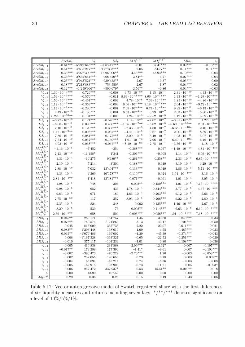
130 CHAPTER 5. THE LEAD-LAG BEHAVIOR
SrelMt Vt D$t MIA,V ∗t MIB,V ∗
t LR3 t rt
SrelMt−1 –0.61*** –5’242’645*** –908’417*** –0.01 37.41*** 0.09*** –0.13***SrelMt−2 –0.51*** –4’605’217*** –1’177’303*** 2.05 34.77** 0.11*** –0.11***SrelMt−3 –0.36*** –4’027’390*** –1’096’006** 4.45*** 43.94*** 0.10*** –0.04SrelMt−4 –0.33*** –2’832’844*** –968’529** 3.84** 4.27 0.07*** –0.04SrelMt−5 –0.25*** –2’943’521*** –939’458** 2.07 19.37 0.05*** 0.00SrelMt−6 –0.18*** –2’218’883*** –753’550* 2.67 1.87 0.04*** –0.02SrelMt−7 –0.12*** –1’259’966** –590’679* 2.56** –0.86 0.04*** –0.03
Vt−1 1.30 · 10−9*** -0.729*** –0.008 4.73 · 10−8* 1.15 · 10−7 2.31 · 10−10 4.43 · 10−10
Vt−2 1.53 · 10−9*** –0.570*** –0.011 8.69 · 10−8*** 8.66 · 10−7*** 1.43 · 10−10 −1.29 · 10−9**Vt−3 1.50 · 10−9*** –0.461*** 0.003 4.78 · 10−8 7.39 · 10−7** 1.85 · 10−10 −4.86 · 10−10
Vt−4 1.12 · 10−9*** –0.369*** –0.003 6.66 · 10−8** 9.18 · 10−7*** 2.04 · 10−10 −9.72 · 10−10*Vt−5 1.14 · 10−9*** –0.280*** –0.007 7.65 · 10−8** 6.74 · 10−7** 9.92 · 10−11 −6.13 · 10−10
Vt−6 4.49 · 10−10 –0.186*** 0.001 6.53 · 10−8** 3.29 · 10−7 2.03 · 10−10 5.80 · 10−11
Vt−7 6.22 · 10−10** –0.101*** 0.006 1.24 · 10−8 −9.52 · 10−8 1.12 · 10−10 5.89 · 10−10
D$t−1 −3.77 · 10−10 0.121*** –0.576*** 1.14 · 10−8 −7.07 · 10−7 −3.81 · 10−10 1.22 · 10−9
D$t−2 −8.08 · 10−11 0.098*** –0.406*** −1.06 · 10−7** −5.02 · 10−8 −6.69 · 10−10** 2.03 · 10−9**D$t−3 7.10 · 10−11 0.120*** –0.308*** −7.33 · 10−8 4.60 · 10−7 −6.38 · 10−10* 2.40 · 10−10
D$t−4 1.47 · 10−9** 0.093*** –0.237*** −4.41 · 10−8 9.67 · 10−7 2.00 · 10−10 8.39 · 10−10
D$t−5 7.86 · 10−10 0.081*** –0.175*** −3.29 · 10−8 3.49 · 10−7 −1.93 · 10−11 5.07 · 10−10
D$t−6 −7.54 · 10−10 0.057*** –0.130*** −1.01 · 10−7* 2.96 · 10−7 −6.40 · 10−10* 6.46 · 10−10
D$t−7 4.93 · 10−10 0.058*** –0.057*** −8.19 · 10−8* −2.75 · 10−7 −3.36 · 10−10 1.18 · 10−9
MIA,V ∗t−1 −1.16 · 10−5 –6’452 –354 –0.368*** 0.057 −1.40 · 10−4* 4.81 · 10−4**
MIA,V ∗t−2 2.43 · 10−4* –11’458* 4’341 –0.303*** –0.005 1.14 · 10−4 6.09 · 10−4**
MIA,V ∗t−3 1.31 · 10−4 –10’275 9’689** –0.261*** 0.358** 2.33 · 10−5 6.85 · 10−4***
MIA,V ∗t−4 2.19 · 10−4 –5’214 3’300 –0.188*** 0.019 3.19 · 10−5 4.20 · 10−4*
MIA,V ∗t−5 2.88 · 10−4* –5’032 13’404*** –0.133*** –0.019 −1.86 · 10−5 5.71 · 10−4**
MIA,V ∗t−6 1.33 · 10−4 –4’369 10’178*** –0.119*** –0.024 1.64 · 10−4** 3.16 · 10−4
MIA,V ∗t−7 2.81 · 10−4** –1’418 13’181*** –0.071*** –0.091 1.01 · 10−4 3.05 · 10−4
MIB,V ∗t−1 1.98 · 10−5 748 –306 0.003** –0.450*** 1.01 · 10−6 −7.13 · 10−5***
MIB,V ∗t−2 9.98 · 10−6 652 –433 4.78 · 10−4 –0.344*** 3.77 · 10−6 −4.67 · 10−5**
MIB,V ∗t−3 −9.83 · 10−6 671 –189 −4.86 · 10−4 –0.263*** 9.12 · 10−6 −5.66 · 10−6
MIB,V ∗t−4 2.75 · 10−5* –117 –352 −8.93 · 10−5 –0.266*** 9.22 · 10−6 −2.80 · 10−5
MIB,V ∗t−5 2.35 · 10−5 –824 –348 –0.002 –0.135*** 1.46 · 10−5* −2.67 · 10−5
MIB,V ∗t−6 8.29 · 10−6 –539 –76 –0.003** –0.114*** 6.63 · 10−6 −6.19 · 10−5***
MIB,V ∗t−7 −2.59 · 10−5** 658 509 –0.003*** –0.056*** 1.91 · 10−5*** −7.18 · 10−5***
LR3 t−1 0.045** 289’171 164’757 –1.45 –33.80 –0.849*** 0.033LR3 t−2 0.072** –760’574 1’121’860 –3.13 –43.17 –0.704*** 0.050LR3 t−3 0.045 –815’099 365’735 –2.22 –20.07 –0.611*** 0.021LR3 t−4 0.083** –1’203’448 –168’619 –1.09 4.55 –0.485*** –0.033LR3 t−5 0.065** –1’079’486 169’002 –1.29 –45.39 –0.374*** –0.043LR3 t−6 0.008 –1’167’328 –363’327 –0.65 –22.52 –0.251*** –0.029LR3 t−7 –0.010 375’117 –101’239 –1.01 0.80 –0.108*** 0.036
rt−1 –0.005 410’838 231’868 –2.09*** –12.62* –0.007 –0.197***rt−2 –0.017** 179’288 177’390 –1.41* –9.61 0.007 –0.103***rt−3 –0.002 –390’473 –70’272 –2.70*** 1.26 –0.003 –0.058***rt−4 –0.002 232’055 –196’656 –0.73 –8.78 0.003 –0.032**rt−5 –0.004 65’894 –45’214 0.74 –5.36 –0.003 –0.008rt−6 –0.005 –62’915 193’900 –0.73 11.21 0.005 –0.023*rt−7 0.006 252’472 332’937* –0.53 15.51** –0.010** 0.018
C 0.00 43.90 107.59 0.00 0.00 0.00 0.00Adj.R2 0.29 0.36 0.26 0.15 0.19 0.43 0.06
Table 5.17: Vector autoregressive model of Swatch registered share with the first differencesof six liquidity measures and returns including seven lags. */**/*** denotes significance ona level of 10%/5%/1%.
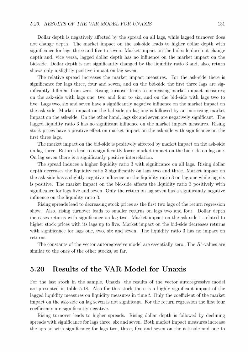
5.20. RESULTS OF THE VAR MODEL FOR UNAXIS 131
Dollar depth is negatively affected by the spread on all lags, while lagged turnover does
not change depth. The market impact on the ask-side leads to higher dollar depth with
significance for lags three and five to seven. Market impact on the bid-side does not change
depth and, vice versa, lagged dollar depth has no influence on the market impact on the
bid-side. Dollar depth is not significantly changed by the liquidity ratio 3 and, also, return
shows only a slightly positive impact on lag seven.
The relative spread increases the market impact measures. For the ask-side there is
significance for lags three, four and seven, and on the bid-side the first three lags are sig-
nificantly different from zero. Rising turnover leads to increasing market impact measures;
on the ask-side with lags one, two and four to six, and on the bid-side with lags two to
five. Lags two, six and seven have a significantly negative influence on the market impact on
the ask-side. Market impact on the bid-side on lag one is followed by an increasing market
impact on the ask-side. On the other hand, lags six and seven are negatively significant. The
lagged liquidity ratio 3 has no significant influence on the market impact measures. Rising
stock prices have a positive effect on market impact on the ask-side with significance on the
first three lags.
The market impact on the bid-side is positively affected by market impact on the ask-side
on lag three. Returns lead to a significantly lower market impact on the bid-side on lag one.
On lag seven there is a significantly positive interrelation.
The spread induces a higher liquidity ratio 3 with significance on all lags. Rising dollar
depth decreases the liquidity ratio 3 significantly on lags two and three. Market impact on
the ask-side has a slightly negative influence on the liquidity ratio 3 on lag one while lag six
is positive. The market impact on the bid-side affects the liquidity ratio 3 positively with
significance for lags five and seven. Only the return on lag seven has a significantly negative
influence on the liquidity ratio 3.
Rising spreads lead to decreasing stock prices as the first two lags of the return regression
show. Also, rising turnover leads to smaller returns on lags two and four. Dollar depth
increases returns with significance on lag two. Market impact on the ask-side is related to
higher stock prices with its lags up to five. Market impact on the bid-side decreases returns
with significance for lags one, two, six and seven. The liquidity ratio 3 has no impact on
returns.
The constants of the vector autoregressive model are essentially zero. The R2-values are
similar to the ones of the other stocks, so far.
5.20 Results of the VAR Model for Unaxis
For the last stock in the sample, Unaxis, the results of the vector autoregressive model
are presented in table 5.18. Also for this stock there is a highly significant impact of the
lagged liquidity measures on liquidity measures in time t. Only the coefficient of the market
impact on the ask-side on lag seven is not significant. For the return regression the first four
coefficients are significantly negative.
Rising turnover leads to higher spreads. Rising dollar depth is followed by declining
spreads with significance for lags three, six and seven. Both market impact measures increase
the spread with significance for lags two, three, five and seven on the ask-side and one to
132 CHAPTER 5. THE LEAD-LAG BEHAVIOR
SrelMt Vt D$t MIA,V ∗t MIB,V ∗
t LR3 t rt
SrelMt−1 –0.64*** –7’834’366*** –523’871 –37.71** 92.61 0.07*** –0.02SrelMt−2 –0.50*** –5’234’656*** –1’338’317** –23.56 –145.86 0.06*** –0.03SrelMt−3 –0.37*** –4’556’078*** –1’459’049*** 4.98 –129.03 0.07*** –0.04SrelMt−4 –0.32*** –3’706’820*** –1’524’205*** 39.19* 365.84*** 0.06*** –0.03SrelMt−5 –0.24*** –3’651’670*** –469’981 29.89 77.65 0.06*** –0.07**SrelMt−6 –0.17*** –2’600’022** –105’217 39.65* 128.38 0.04*** –0.01SrelMt−7 –0.08*** –1’193’057 –28’006 30.39* 347.91*** 0.03*** 0.01
Vt−1 5.41 · 10−10*** –0.716*** 0.009* −2.00 · 10−8 9.53 · 10−7 2.18 · 10−10** −3.43 · 10−10
Vt−2 8.34 · 10−10*** –0.587*** 0.007 −1.29 · 10−7 1.55 · 10−6 2.78 · 10−10** −3.28 · 10−10
Vt−3 7.91 · 10−10*** –0.447*** –0.003 5.58 · 10−8 8.52 · 10−7 3.88 · 10−10*** 6.93 · 10−11
Vt−4 6.58 · 10−10*** –0.347*** –0.004 3.74 · 10−7 9.71 · 10−8 4.24 · 10−10*** 1.14 · 10−10
Vt−5 6.33 · 10−10*** –0.282*** 0.006 5.54 · 10−7* 1.98 · 10−7 2.14 · 10−10* −2.16 · 10−10
Vt−6 5.99 · 10−10*** –0.219*** –0.001 2.74 · 10−7 −7.19 · 10−7 2.17 · 10−10* −4.29 · 10−10
Vt−7 4.81 · 10−10*** –0.112*** –0.002 1.84 · 10−7 −3.70 · 10−7 1.64 · 10−10* −1.35 · 10−10
D$t−1 −3.07 · 10−10 0.239*** –0.583*** 1.37 · 10−6** −7.76 · 10−7 −3.51 · 10−10 1.07 · 10−9
D$t−2 −6.30 · 10−10 0.184*** –0.410*** 1.55 · 10−6** −7.05 · 10−7 −4.48 · 10−10 8.26 · 10−10
D$t−3 −1.19 · 10−9** 0.169*** –0.350*** 1.01 · 10−6 −6.09 · 10−7 −5.29 · 10−10* 5.78 · 10−10
D$t−4 −6.38 · 10−10 0.143*** –0.298*** 7.44 · 10−7 −3.72 · 10−6 −5.08 · 10−10* −3.35 · 10−10
D$t−5 −7.59 · 10−10 0.191*** –0.220*** 1.21 · 10−7 −5.59 · 10−6 −3.98 · 10−10 4.62 · 10−10
D$t−6 −9.84 · 10−10** 0.123*** –0.177*** 4.68 · 10−8 −6.76 · 10−6* −5.94 · 10−10** 6.72 · 10−10
D$t−7 −1.53 · 10−9*** 0.047 –0.118*** −3.70 · 10−7 −1.05 · 10−5*** −7.05 · 10−10*** 9.40 · 10−10
MIA,V ∗t−1 1.34 · 10−6 –878 –173 –0.353*** –0.008 2.39 · 10−5*** 9.25 · 10−6
MIA,V ∗t−2 2.29 · 10−5** –590 –50 –0.180*** –0.047 1.67 · 10−5*** 2.60 · 10−5
MIA,V ∗t−3 2.12 · 10−5** –35 –107 –0.133*** 0.065 2.83 · 10−6 1.57 · 10−5
MIA,V ∗t−4 1.60 · 10−5 –1’223 –7 –0.079*** 0.130 4.98 · 10−6 2.77 · 10−5
MIA,V ∗t−5 2.90 · 10−5*** –694 –230 –0.053*** –0.088 1.03 · 10−5* 3.40 · 10−5**
MIA,V ∗t−6 5.50 · 10−6 –59 –528* –0.034** 0.003 2.66 · 10−6 1.25 · 10−5
MIA,V ∗t−7 2.46 · 10−5*** –1’015 –217 –0.009 0.030 4.06 · 10−6 3.50 · 10−5**
MIB,V ∗t−1 5.27 · 10−6*** –56 –2 0.001 –0.362*** 9.66 · 10−7 −6.27 · 10−6**
MIB,V ∗t−2 4.76 · 10−6*** 47 –9 –0.002 –0.176*** 1.61 · 10−6 −6.20 · 10−6**
MIB,V ∗t−3 3.88 · 10−6** –67 6 0.001 –0.138*** 5.36 · 10−7 −1.96 · 10−6
MIB,V ∗t−4 2.52 · 10−6 –51 9 –0.002 –0.069*** 4.05 · 10−7 −4.99 · 10−6*
MIB,V ∗t−5 7.01 · 10−7 –21 –45 –0.001 –0.039*** 1.37 · 10−6 −4.78 · 10−7
MIB,V ∗t−6 3.39 · 10−6** –33 58 –0.007*** –0.076*** 1.55 · 10−7 −2.85 · 10−7
MIB,V ∗t−7 1.89 · 10−6 65 1 −2.61 · 10−4 –0.059*** −1.12 · 10−6 −2.39 · 10−6
LR3 t−1 –0.004 –913’725 –1’141’430* –63.76** 33.16 –0.816*** 0.007LR3 t−2 0.009 –704’756 –488’864 –59.95 242.48 –0.660*** 0.013LR3 t−3 0.004 –2’412’198 –61’228 –31.84 –55.22 –0.547*** –0.016LR3 t−4 –0.006 1’210’456 –1’355’956 –46.68 165.59 –0.448*** –0.062LR3 t−5 –0.036 129’350 –1’977’427** –60.77 –30.51 –0.318*** –0.023LR3 t−6 –0.008 –154’874 –1’605’420* –76.54** –95.19 –0.236*** –0.044LR3 t−7 0.012 –408’235 –767’422 –44.59 35.71 –0.122*** –0.009
rt−1 –0.003 1’269’623** 166’531 –11.23 –83.70 0.002 –0.165***rt−2 –0.008 715’702 106’104 –28.44*** –11.71 0.004 –0.044***rt−3 –0.008 –38’810 328’718 –7.80 83.23 0.008* –0.038***rt−4 –0.001 195’042 –70’173 –16.24 125.79** –0.005 –0.040***rt−5 –0.008 108’410 –172’222 29.38*** 288.73*** –0.002 –0.016rt−6 –0.014* –367’570 –175’209 1.92 65.26 –0.003 0.001rt−7 0.011 –538’348 68’664 4.38 –14.06 –0.007* 0.006
C 0.00 142.06 –7.40 0.00 0.01 0.00 0.00Adj.R2 0.29 0.36 0.27 0.12 0.13 0.40 0.03
Table 5.18: Vector autoregressive model of Unaxis with the first differences of six liquiditymeasures and returns including seven lags. */**/*** denotes significance on a level of10%/5%/1%.
5.21. GENERAL RESULTS OF THE VAR MODEL 133
three and six on the bid-side. The liquidity ratio 3 has no significant impact on the relative
spread, while all lags of the relative spread are highly significant with respect to the liquidity
ratio 3. Only returns on lag six have a slightly negative impact on the relative spread.
Turnover depends heavily on relative spreads up to lag six. The same holds for the effect
of lagged dollar depth on turnover. The market impact measures do not influence turnover
significantly. In the other direction from lagged turnover to the market impacts, there is only
a slightly positive significance on the ask-side. The lagged liquidity ratio 3 has no impact
on turnover. Return on lag one leads to a significantly higher turnover in time t.
The relative spread is related to lower dollar depth on lags two to four. Turnover has only
a slightly positive influence on depth with lag one. Depth, almost, does not depend on the
market impact measures. There is only a small significance for lag six of the market impact
on the ask-side. The liquidity ratio 3 is followed by a declining dollar depth, with significance
for lags one, five and six. Between dollar depth and returns there is no interrelation in either
direction.
The first lag of the relative spread decreases market impact on the ask-side, while lags
four, six and seven show a slightly positive significance. Market impact depends positively
on the first two lags of dollar depth. Lag six of the market impact on the bid-side is related
to a declining market impact on the ask-side. The liquidity ratio 3 decreases market impact
on the ask-side, with significance for lags one and six. Return has a negative influence on
lag two with respect to market impact on the ask-side, while lag five is significantly positive.
Lags four and seven of the relative spread are related to a rising market impact on the
bid-side. Rising dollar depth leads to a decrease in market impact on the bid-side, as lags
six and seven show. Market impact on the ask-side has no significant influence on market
impact on the bid-side. There is no interrelation of market impact on the bid-side and the
liquidity ratio 3 in both directions. Rising stock prices lead to a rise in market impact on
the bid-side as lags four and five show.
Rising turnover is followed by a rising liquidity ratio 3 with significance on all lags. An
increase in dollar depth is related to a smaller liquidity ratio 3, with significance for lags
three, four, six and seven. Market impact on the ask-side has a positive effect on the liquidity
ratio 3, as lags one, two and five show. There is only slight significance for the impact of
returns on the liquidity ratio 3.
The relative spread is related to negative returns with significance on lag five. Lagged
turnover does not influence returns. Market impact on the ask-side leads to rising stock
prices on lags five and seven. Similarly, market impact on the bid-side leads to declining
returns with significance for lags one, two and four. The liquidity ratio 3 does not affect
returns significantly.
All the constants of the vector autoregressive model are virtually zero and the adjusted
R2-values are in line with the other stocks.
5.21 General Results of the Vector Autoregressive Model
The following interrelations among the seven variables of the vector autoregressive model
hold more or less across all the eighteen stocks:
• All the changes in liquidity measures depend negatively on their own lags.
134 CHAPTER 5. THE LEAD-LAG BEHAVIOR
Since there is high autocorrelation among the variables, they do not follow a random
walk but tend to return to their long range mean.
• The relative spread is positively influenced by turnover.
Increasing trading activity due to market orders (or marketable limit orders) cancels
the best bid and ask quotes and leads, therefore, to a higher spread.
• The market impact measures increase the spread.
Due to a thin order book on one or the other side of the order book, trades delete the
best bid or ask quote more rapidly and the spread rises.
• Turnover depends negatively on the relative spread.
A higher spread makes trading more costly and causes, therefore, less turnover.
• Dollar depth increases turnover.
The same argument as above holds: a high depth makes trading cheaper and causes,
therefore, higher turnover.
• The market impact on the ask-side decreases turnover.
If the market impact is high, larger trades become more expensive because they have
to walk the book to be executed. Therefore, market impact induces less turnover. For
market impact on the bid-side the effect is not that clear.
• A rising spread decreases dollar depth.
This effect is more difficult to justify from an economic point of view. One explana-
tion may be that, since a large spread is a sign of uncertainty in the market, market
participants may be more prudent and reduce there positions at the best bid and ask
quotes.
• Rising turnover increases the market impact on the bid- and the ask-side.
Higher turnover, due to market orders, takes depth away and leads, therefore, to higher
market impacts.
• Rising Market impact on the ask-side increases market impact on the bid-side.
In the other direction, the effect is not very pronounced. The asymmetry of this
empirical finding is difficult to explain. Increased trading activity in the market may
lead to a thinner order book on both sides of the market, but there is no reason for
the one side of the market to react first.
• A rising relative spread leads to a larger liquidity ratio 3.
Since the rising spread decreases turnover the liquidity ratio 3 must rise.
• Market impact on the bid-side leads to a larger liquidity ratio 3.
Fewer stocks show this effect for the market impact on the ask-side. Since the liquidity
ratio 3 is calculated with the absolute return in the numerator it is difficult to justify
why the effect is different for the bid- and the ask-side of the order book.

5.21. GENERAL RESULTS OF THE VAR MODEL 135
• Market impact on the ask-side leads to higher stock prices; market impact on the
bid-side makes stock prices decline.
If liquidity on the ask-side of the order book is already scarce, subsequent market
orders lead to higher stock prices. For the bid-side the opposite holds.
• All of the constants of the vector autoregressive model are zero.
Since the model is built with the differences of the liquidity measures and there is no
trend in liquidity the constants must be zero.

136 CHAPTER 5. THE LEAD-LAG BEHAVIOR
Chapter 6
Prediction Models for the Liquidity
Measures
From the vector autoregressive model we have hints which variables are leading indicators
for the liquidity measures. In this chapter linear models are built to predict the liquidity
measures. First, the parameters are estimated using a sliding window of 300 data points
which corresponds to an estimation period of three days. Then the prediction of the changes
in the liquidity measure is calculated with the estimated coefficients. The methodology is
similar to Wang (2002). To determine the fit of the models I calculate the mean squared
errors of the prediction, as described in Hamilton (1994), instead of the adjusted R2-values.
The models are compared to two benchmarks: I calculate the mean squared error of an
adaptive expectation which takes the change of the liquidity measures in time t as prediction
for time t + 1. Since the first differences of the liquidity measures show negative autocorre-
lation, I additionally calculate the mean squared error between the negative change of the
liquidity measure in time t and the change in t + 1.
6.1 Predicting the Relative Spread
The results from the vector autoregressive model across the 18 stocks show that the relative
spread depends negatively on the lagged spread itself. The dependence on turnover and
the market impact measures is mainly positive, while the return has a negative impact.
Therefore, these five variables are included in the model. I propose three different models
which use a different number of lags to estimate the regression parameters.
Model 1, which is shown in equation 6.1, includes the spread, turnover, market impact
on the ask- and on the bid-side and returns of the first lag:
dSrelMt = c + β1 · dSrelMt−1 + β2 · dVt−1 + β3 · dMIA,V ∗t−1
+ β4 · dMIB,V ∗t−1 + β5 · rt−1 + ε (6.1)
In addition to model 1, the second model in equation 6.2 includes the second lag of the
relative spread and of turnover.
137
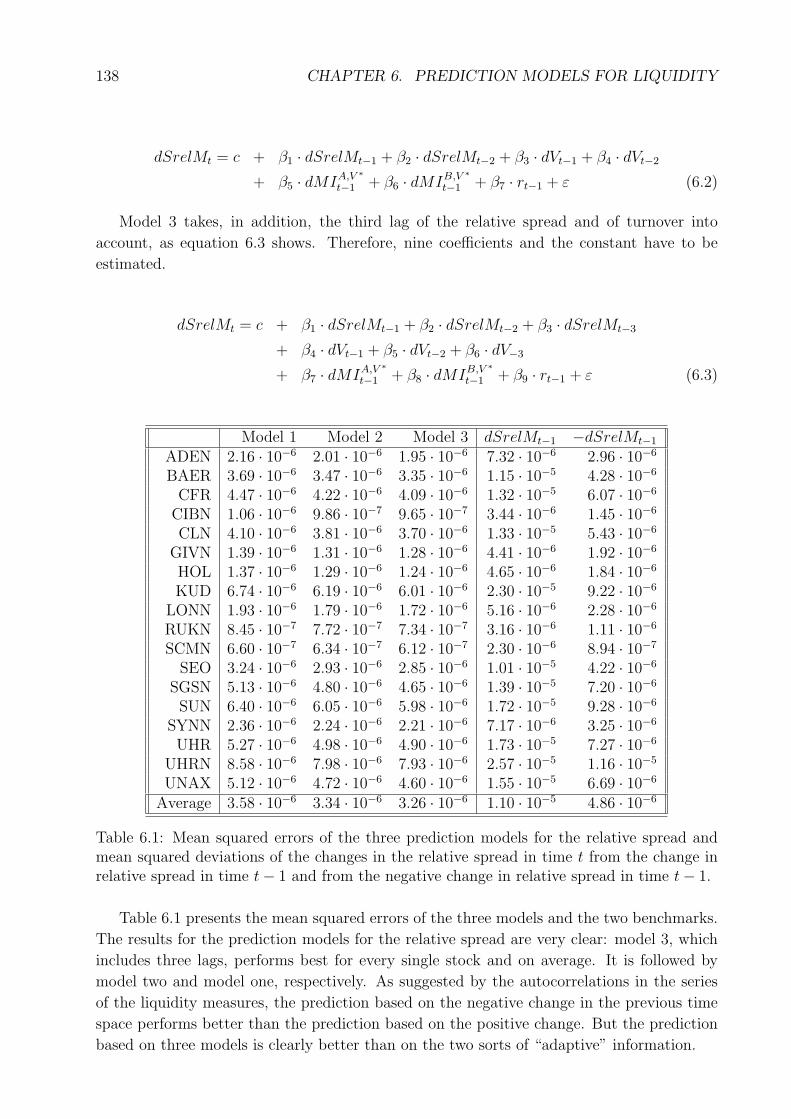
138 CHAPTER 6. PREDICTION MODELS FOR LIQUIDITY
dSrelMt = c + β1 · dSrelMt−1 + β2 · dSrelMt−2 + β3 · dVt−1 + β4 · dVt−2
+ β5 · dMIA,V ∗t−1 + β6 · dMIB,V ∗
t−1 + β7 · rt−1 + ε (6.2)
Model 3 takes, in addition, the third lag of the relative spread and of turnover into
account, as equation 6.3 shows. Therefore, nine coefficients and the constant have to be
estimated.
dSrelMt = c + β1 · dSrelMt−1 + β2 · dSrelMt−2 + β3 · dSrelMt−3
+ β4 · dVt−1 + β5 · dVt−2 + β6 · dV−3
+ β7 · dMIA,V ∗t−1 + β8 · dMIB,V ∗
t−1 + β9 · rt−1 + ε (6.3)
Model 1 Model 2 Model 3 dSrelMt−1 −dSrelMt−1
ADEN 2.16 · 10−6 2.01 · 10−6 1.95 · 10−6 7.32 · 10−6 2.96 · 10−6
BAER 3.69 · 10−6 3.47 · 10−6 3.35 · 10−6 1.15 · 10−5 4.28 · 10−6
CFR 4.47 · 10−6 4.22 · 10−6 4.09 · 10−6 1.32 · 10−5 6.07 · 10−6
CIBN 1.06 · 10−6 9.86 · 10−7 9.65 · 10−7 3.44 · 10−6 1.45 · 10−6
CLN 4.10 · 10−6 3.81 · 10−6 3.70 · 10−6 1.33 · 10−5 5.43 · 10−6
GIVN 1.39 · 10−6 1.31 · 10−6 1.28 · 10−6 4.41 · 10−6 1.92 · 10−6
HOL 1.37 · 10−6 1.29 · 10−6 1.24 · 10−6 4.65 · 10−6 1.84 · 10−6
KUD 6.74 · 10−6 6.19 · 10−6 6.01 · 10−6 2.30 · 10−5 9.22 · 10−6
LONN 1.93 · 10−6 1.79 · 10−6 1.72 · 10−6 5.16 · 10−6 2.28 · 10−6
RUKN 8.45 · 10−7 7.72 · 10−7 7.34 · 10−7 3.16 · 10−6 1.11 · 10−6
SCMN 6.60 · 10−7 6.34 · 10−7 6.12 · 10−7 2.30 · 10−6 8.94 · 10−7
SEO 3.24 · 10−6 2.93 · 10−6 2.85 · 10−6 1.01 · 10−5 4.22 · 10−6
SGSN 5.13 · 10−6 4.80 · 10−6 4.65 · 10−6 1.39 · 10−5 7.20 · 10−6
SUN 6.40 · 10−6 6.05 · 10−6 5.98 · 10−6 1.72 · 10−5 9.28 · 10−6
SYNN 2.36 · 10−6 2.24 · 10−6 2.21 · 10−6 7.17 · 10−6 3.25 · 10−6
UHR 5.27 · 10−6 4.98 · 10−6 4.90 · 10−6 1.73 · 10−5 7.27 · 10−6
UHRN 8.58 · 10−6 7.98 · 10−6 7.93 · 10−6 2.57 · 10−5 1.16 · 10−5
UNAX 5.12 · 10−6 4.72 · 10−6 4.60 · 10−6 1.55 · 10−5 6.69 · 10−6
Average 3.58 · 10−6 3.34 · 10−6 3.26 · 10−6 1.10 · 10−5 4.86 · 10−6
Table 6.1: Mean squared errors of the three prediction models for the relative spread andmean squared deviations of the changes in the relative spread in time t from the change inrelative spread in time t− 1 and from the negative change in relative spread in time t− 1.
Table 6.1 presents the mean squared errors of the three models and the two benchmarks.
The results for the prediction models for the relative spread are very clear: model 3, which
includes three lags, performs best for every single stock and on average. It is followed by
model two and model one, respectively. As suggested by the autocorrelations in the series
of the liquidity measures, the prediction based on the negative change in the previous time
space performs better than the prediction based on the positive change. But the prediction
based on three models is clearly better than on the two sorts of “adaptive” information.
6.2. PREDICTING TURNOVER 139
6.2 Predicting Turnover
As well as for the relative spread, three models are built for turnover and compared against
each other and against turnover in the preceding time space. From the vector autoregressive
model we know that turnover depends primarily on lagged turnover and relative spread
negatively, and on dollar depth positively. The influence of the market impact measures is
predominantly negative but not so clear-cut.
These five liquidity measures are used to predict turnover and model 1 includes the first
lags:
dVt = c + β1 · dVt−1 + β2 · dSrelMt−1 + β3 · dD$t−1
+ β4 · dMIA,V ∗t−1 + β5 · dMIB,V ∗
t−1 + ε (6.4)
In model 2 the second lags of turnover, relative spread and dollar depth are included.
Since the influence of the market impact measures is not always clear, their second lags are
left out. Therefore, model 2 includes eight variables:
dVt = c + β1 · dVt−1 + β2 · dVt−2 + β3 · dSrelMt−1 + β4 · dSrelMt−2
+ β5 · dD$t−1 + β6 · dD$t−2
+ β7dMIA,V ∗t−1 + β8 · dMIB,V ∗
t−1 + ε (6.5)
In addition to model 2, model 3 includes the third lags of turnover, relative spread and
dollar depth:
dVt = c + β1 · dVt−1 + β2 · dVt−2 + β3 · dVt−3
+ β4 · dSrelMt−1 + β5 · dSrelMt−2 + β6 · dSrelMt−3
+ β7 · dD$t−1 + β8 · dD$t−2 + β9 · dD$t−3
+ β10 · dMIA,V ∗t−1 + β11 · dMIB,V ∗
t−1 + ε (6.6)
Table 6.2 presents the mean squared errors of the prediction models for turnover with
the respective benchmarks.
For sixteen of the eighteen stocks, model 3 performs best and has the smallest mean
squared errors, on average. For Adecco, model 2, with only two lags included, shows the
best results. For Surveillance it is the negative turnover in time t that is the best predictor
for turnover in t + 1.
6.3 Predicting Dollar Depth
The results of the vector autoregressive model for dollar depth show a clearly negative
dependence on dollar depth itself as well as on the relative spread. The influence of the
other liquidity measures and returns is ambiguous across the 18 stocks. Therefore, only two
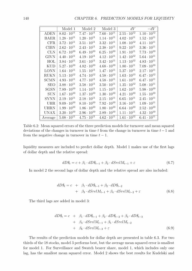
140 CHAPTER 6. PREDICTION MODELS FOR LIQUIDITY
Model 1 Model 2 Model 3 dV −dVADEN 8.02 · 1011 7.47 · 1011 7.60 · 1011 2.55 · 1012 1.10 · 1012
BAER 1.28 · 1011 1.20 · 1011 1.14 · 1011 4.02 · 1011 1.52 · 1011
CFR 3.72 · 1011 3.51 · 1011 3.32 · 1011 1.08 · 1012 4.11 · 1011
CIBN 2.62 · 1011 2.43 · 1011 2.38 · 1011 9.22 · 1011 3.36 · 1011
CLN 6.72 · 1010 6.49 · 1010 6.25 · 1010 1.91 · 1011 7.73 · 1010
GIVN 4.40 · 1011 4.19 · 1011 4.12 · 1011 1.42 · 1012 5.64 · 1011
HOL 3.84 · 1011 3.61 · 1011 3.42 · 1011 1.13 · 1012 4.83 · 1011
KUD 5.27 · 1010 4.82 · 1010 4.68 · 1010 1.80 · 1011 7.09 · 1010
LONN 1.64 · 1011 1.55 · 1011 1.47 · 1011 5.37 · 1011 2.17 · 1011
RUKN 5.13 · 1012 4.74 · 1012 4.58 · 1012 1.63 · 1013 6.47 · 1012
SCMN 4.93 · 1011 4.77 · 1011 4.58 · 1011 1.61 · 1012 6.47 · 1011
SEO 3.88 · 1011 3.58 · 1011 3.50 · 1011 1.35 · 1012 5.08 · 1011
SGSN 7.89 · 1010 1.14 · 1011 1.15 · 1011 1.62 · 1011 5.98 · 1010
SUN 1.67 · 1010 1.37 · 1010 1.30 · 1010 4.21 · 1010 1.55 · 1010
SYNN 2.19 · 1011 2.18 · 1011 2.15 · 1011 6.65 · 1011 2.45 · 1011
UHR 9.09 · 1010 8.10 · 1010 7.92 · 1010 3.16 · 1011 1.09 · 1011
UHRN 1.99 · 1010 1.86 · 1010 1.80 · 1010 6.64 · 1010 2.52 · 1010
UNAX 3.20 · 1010 2.96 · 1010 2.89 · 1010 1.11 · 1011 4.32 · 1010
Average 5.08 · 1011 4.75 · 1011 4.62 · 1011 1.61 · 1012 6.41 · 1011
Table 6.2: Mean squared errors of the three prediction models for turnover and mean squareddeviations of the changes in turnover in time t from the change in turnover in time t− 1 andfrom the negative change in turnover in time t− 1.
liquidity measures are included to predict dollar depth. Model 1 makes use of the first lags
of dollar depth and the relative spread:
dD$t = c + β1 · dD$t−1 + β2 · dSrelMt−1 + ε (6.7)
In model 2 the second lags of dollar depth and the relative spread are also included:
dD$t = c + β1 · dD$t−1 + β2 · dD$t−2
+ β3 · dSrelMt−1 + β4 · dSrelMt−2 + ε (6.8)
The third lags are added in model 3:
dD$t = c + β1 · dD$t−1 + β2 · dD$t−2 + β3 · dD$t−3
+ β4 · dSrelMt−1 + β5 · dSrelMt−2
+ β6 · dSrelMt−3 + ε (6.9)
The results of the prediction models for dollar depth are presented in table 6.3. For two
thirds of the 18 stocks, model 3 performs best, but the average mean squared error is smallest
for model 1. For Surveillance and Swatch bearer share, model 1, which includes only one
lag, has the smallest mean squared error. Model 2 shows the best results for Kudelski and
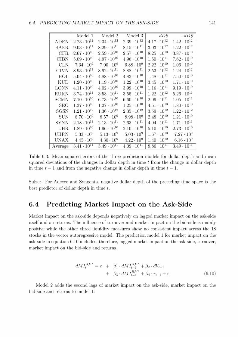
6.4. PREDICTING MARKET IMPACT ON THE ASK-SIDE 141
Model 1 Model 2 Model 3 dD$ −dD$ADEN 2.23 · 1012 2.34 · 1012 2.39 · 1012 4.17 · 1012 1.42 · 1012
BAER 9.03 · 1011 8.29 · 1011 8.15 · 1011 3.03 · 1012 1.22 · 1012
CFR 2.67 · 1010 2.59 · 1010 2.57 · 1010 8.25 · 1010 3.87 · 1010
CIBN 5.09 · 1010 4.97 · 1010 4.96 · 1010 1.50 · 1011 7.62 · 1010
CLN 7.34 · 109 7.00 · 109 6.88 · 109 2.22 · 1010 1.06 · 1010
GIVN 8.93 · 1011 8.92 · 1011 8.88 · 1011 2.53 · 1012 1.24 · 1012
HOL 5.04 · 1010 4.88 · 1010 4.83 · 1010 1.48 · 1011 7.50 · 1010
KUD 1.20 · 1010 1.19 · 1010 1.22 · 1010 3.45 · 1010 1.71 · 1010
LONN 4.11 · 1010 4.02 · 1010 3.99 · 1010 1.16 · 1011 9.19 · 1010
RUKN 3.74 · 1011 3.58 · 1011 3.55 · 1011 1.22 · 1012 5.26 · 1011
SCMN 7.10 · 1010 6.73 · 1010 6.60 · 1010 2.09 · 1011 1.05 · 1011
SEO 1.37 · 1010 1.27 · 1010 1.25 · 1010 4.51 · 1010 1.80 · 1010
SGSN 1.21 · 1012 1.36 · 1012 2.35 · 1012 3.59 · 1012 1.22 · 1012
SUN 8.70 · 109 8.57 · 109 8.98 · 109 2.48 · 1010 1.21 · 1010
SYNN 2.18 · 1011 2.13 · 1011 2.63 · 1011 4.94 · 1011 1.71 · 1011
UHR 1.89 · 1010 1.96 · 1010 2.10 · 1010 5.10 · 1010 2.73 · 1010
UHRN 5.33 · 109 5.13 · 109 5.03 · 109 1.67 · 1010 7.27 · 109
UNAX 4.45 · 109 4.30 · 109 4.22 · 109 1.40 · 1010 6.16 · 109
Average 3.41 · 1011 3.49 · 1011 4.09 · 1011 8.86 · 1011 3.49 · 1011
Table 6.3: Mean squared errors of the three prediction models for dollar depth and meansquared deviations of the changes in dollar depth in time t from the change in dollar depthin time t− 1 and from the negative change in dollar depth in time t− 1.
Sulzer. For Adecco and Syngenta, negative dollar depth of the preceding time space is the
best predictor of dollar depth in time t.
6.4 Predicting Market Impact on the Ask-Side
Market impact on the ask-side depends negatively on lagged market impact on the ask-side
itself and on returns. The influence of turnover and market impact on the bid-side is mainly
positive while the other three liquidity measures show no consistent impact across the 18
stocks in the vector autoregressive model. The prediction model 1 for market impact on the
ask-side in equation 6.10 includes, therefore, lagged market impact on the ask-side, turnover,
market impact on the bid-side and returns.
dMIA,V ∗t = c + β1 · dMIA,V ∗
t−1 + β2 · dVt−1
+ β3 · dMIB,V ∗t−1 + β4 · rt−1 + ε (6.10)
Model 2 adds the second lags of market impact on the ask-side, market impact on the
bid-side and returns to model 1:
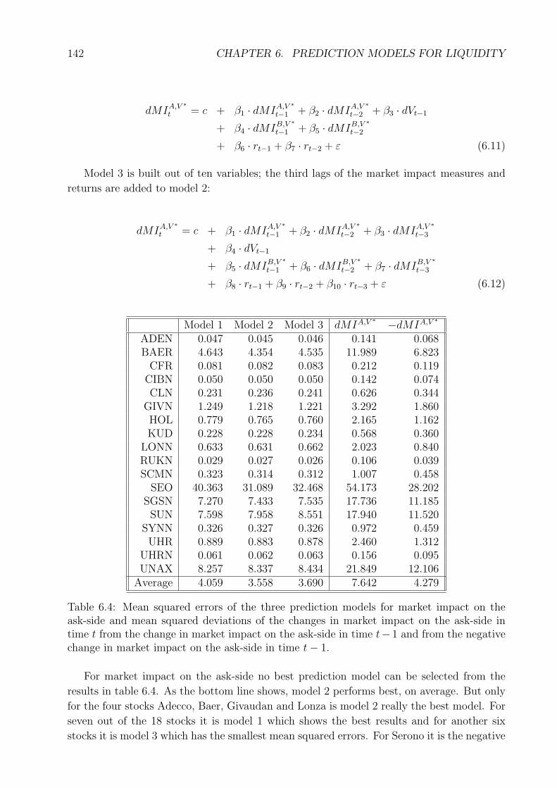
142 CHAPTER 6. PREDICTION MODELS FOR LIQUIDITY
dMIA,V ∗t = c + β1 · dMIA,V ∗
t−1 + β2 · dMIA,V ∗t−2 + β3 · dVt−1
+ β4 · dMIB,V ∗t−1 + β5 · dMIB,V ∗
t−2
+ β6 · rt−1 + β7 · rt−2 + ε (6.11)
Model 3 is built out of ten variables; the third lags of the market impact measures and
returns are added to model 2:
dMIA,V ∗t = c + β1 · dMIA,V ∗
t−1 + β2 · dMIA,V ∗t−2 + β3 · dMIA,V ∗
t−3
+ β4 · dVt−1
+ β5 · dMIB,V ∗t−1 + β6 · dMIB,V ∗
t−2 + β7 · dMIB,V ∗t−3
+ β8 · rt−1 + β9 · rt−2 + β10 · rt−3 + ε (6.12)
Model 1 Model 2 Model 3 dMIA,V ∗ −dMIA,V ∗
ADEN 0.047 0.045 0.046 0.141 0.068BAER 4.643 4.354 4.535 11.989 6.823
CFR 0.081 0.082 0.083 0.212 0.119CIBN 0.050 0.050 0.050 0.142 0.074CLN 0.231 0.236 0.241 0.626 0.344
GIVN 1.249 1.218 1.221 3.292 1.860HOL 0.779 0.765 0.760 2.165 1.162KUD 0.228 0.228 0.234 0.568 0.360
LONN 0.633 0.631 0.662 2.023 0.840RUKN 0.029 0.027 0.026 0.106 0.039SCMN 0.323 0.314 0.312 1.007 0.458
SEO 40.363 31.089 32.468 54.173 28.202SGSN 7.270 7.433 7.535 17.736 11.185SUN 7.598 7.958 8.551 17.940 11.520
SYNN 0.326 0.327 0.326 0.972 0.459UHR 0.889 0.883 0.878 2.460 1.312
UHRN 0.061 0.062 0.063 0.156 0.095UNAX 8.257 8.337 8.434 21.849 12.106
Average 4.059 3.558 3.690 7.642 4.279
Table 6.4: Mean squared errors of the three prediction models for market impact on theask-side and mean squared deviations of the changes in market impact on the ask-side intime t from the change in market impact on the ask-side in time t− 1 and from the negativechange in market impact on the ask-side in time t− 1.
For market impact on the ask-side no best prediction model can be selected from the
results in table 6.4. As the bottom line shows, model 2 performs best, on average. But only
for the four stocks Adecco, Baer, Givaudan and Lonza is model 2 really the best model. For
seven out of the 18 stocks it is model 1 which shows the best results and for another six
stocks it is model 3 which has the smallest mean squared errors. For Serono it is the negative
6.5. PREDICTING MARKET IMPACT ON THE BID-SIDE 143
market impact on the ask-side which yields the best prediction. This may be due to the
extraordinarily high mean squared errors that the models show for Serono. The reason for
the bad performance of the prediction models is the temporarily very thin order book which
leads to huge changes in market impact on the ask-side.
6.5 Predicting Market Impact on the Bid-Side
For the prediction models of market impact on the bid-side, the same variables are included
as for the market impact on the ask-side models. Model 1 in equation 6.13 is, therefore,
built out of the first lags of market impact on the bid-side, turnover, market impact on the
ask-side and returns.
dMIB,V ∗t = c + β1 · dMIB,V ∗
t−1 + β2 · dVt−1
+ β3 · dMIA,V ∗t−1 + β4 · rt−1 + ε (6.13)
Model 2 includes, in addition to model 1, the second lags of market impact on the bid-side,
market impact on the ask-side and returns:
dMIB,V ∗t = c + β1 · dMIB,V ∗
t−1 + β2 · dMIB,V ∗t−2 + β3 · dVt−1
+ β4 · dMIA,V ∗t−1 + β5 · dMIA,V ∗
t−2
+ β6 · rt−1 + β7 · rt−2 + ε (6.14)
Model 3 with ten variables takes also the third lags of market impact on the bid-side,
market impact on the ask-side and returns into account:
dMIB,V ∗t = c + β1 · dMIB,V ∗
t−1 + β2 · dMIB,V ∗t−2 + β3 · dMIB,V ∗
t−3
+ β4 · dVt−1
+ β5 · dMIA,V ∗t−1 + β6 · dMIA,V ∗
t−2 + β7 · dMIA,V ∗t−3
+ β8 · rt−1 + β9 · rt−2 + β10 · rt−3 + ε (6.15)
The mean squared errors for the prediction models of market impact on the bid-side in
table 6.5 are much larger than on the ask-side. This is due to temporarily very low liquidity
on the bid-side which led to huge changes in the bid-side-specific liquidity measure. The
general picture is the same as for the ask-side: there is no model that is superior with
respect to the others. On average, the negative change in market impact on the bid-side in
time t is the best predictor of market impact on the bid-side in t+1. This result stems from
the very poor performance of the other models for the Serono stock. If Serono had been
excluded from the sample, model 2 would perform best. Aside from Serono, the negative
change in market impact on the bid-side is the best predictor only for Lonza. Models 1 and
3 each show the best results for five of the 18 stocks. Model 2 is superior for six of the 18
stocks.
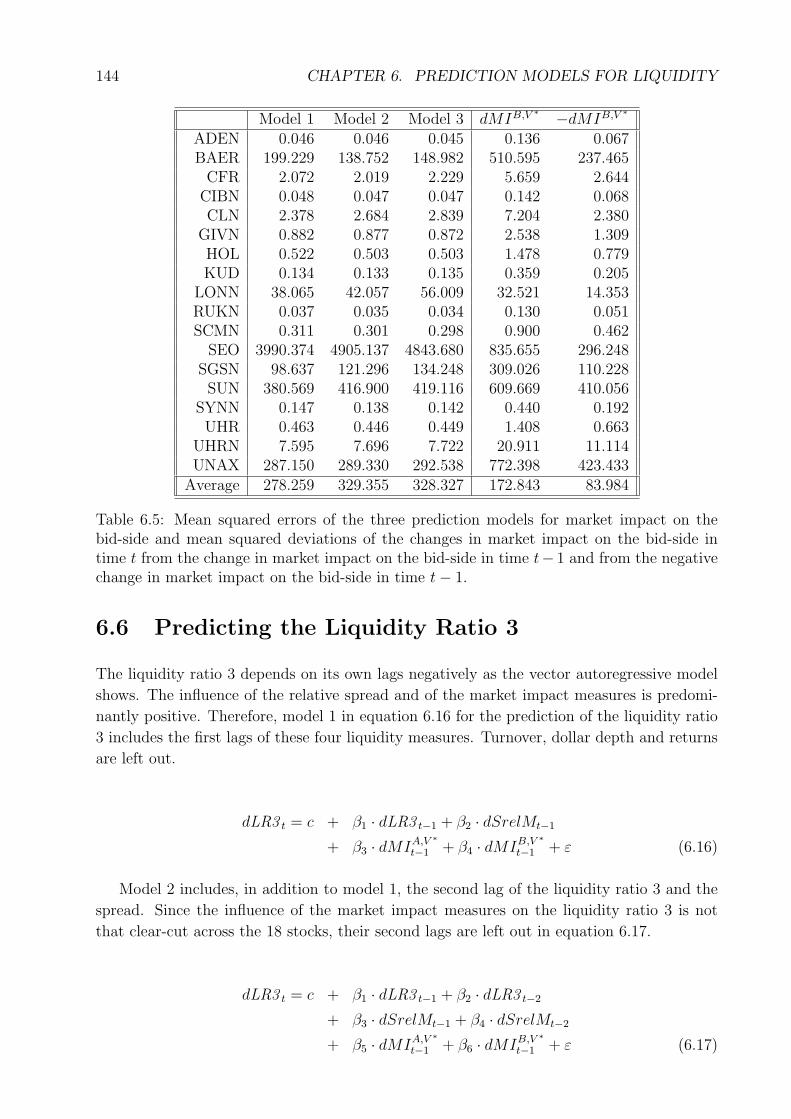
144 CHAPTER 6. PREDICTION MODELS FOR LIQUIDITY
Model 1 Model 2 Model 3 dMIB,V ∗ −dMIB,V ∗
ADEN 0.046 0.046 0.045 0.136 0.067BAER 199.229 138.752 148.982 510.595 237.465
CFR 2.072 2.019 2.229 5.659 2.644CIBN 0.048 0.047 0.047 0.142 0.068CLN 2.378 2.684 2.839 7.204 2.380
GIVN 0.882 0.877 0.872 2.538 1.309HOL 0.522 0.503 0.503 1.478 0.779KUD 0.134 0.133 0.135 0.359 0.205
LONN 38.065 42.057 56.009 32.521 14.353RUKN 0.037 0.035 0.034 0.130 0.051SCMN 0.311 0.301 0.298 0.900 0.462
SEO 3990.374 4905.137 4843.680 835.655 296.248SGSN 98.637 121.296 134.248 309.026 110.228SUN 380.569 416.900 419.116 609.669 410.056
SYNN 0.147 0.138 0.142 0.440 0.192UHR 0.463 0.446 0.449 1.408 0.663
UHRN 7.595 7.696 7.722 20.911 11.114UNAX 287.150 289.330 292.538 772.398 423.433
Average 278.259 329.355 328.327 172.843 83.984
Table 6.5: Mean squared errors of the three prediction models for market impact on thebid-side and mean squared deviations of the changes in market impact on the bid-side intime t from the change in market impact on the bid-side in time t− 1 and from the negativechange in market impact on the bid-side in time t− 1.
6.6 Predicting the Liquidity Ratio 3
The liquidity ratio 3 depends on its own lags negatively as the vector autoregressive model
shows. The influence of the relative spread and of the market impact measures is predomi-
nantly positive. Therefore, model 1 in equation 6.16 for the prediction of the liquidity ratio
3 includes the first lags of these four liquidity measures. Turnover, dollar depth and returns
are left out.
dLR3 t = c + β1 · dLR3 t−1 + β2 · dSrelMt−1
+ β3 · dMIA,V ∗t−1 + β4 · dMIB,V ∗
t−1 + ε (6.16)
Model 2 includes, in addition to model 1, the second lag of the liquidity ratio 3 and the
spread. Since the influence of the market impact measures on the liquidity ratio 3 is not
that clear-cut across the 18 stocks, their second lags are left out in equation 6.17.
dLR3 t = c + β1 · dLR3 t−1 + β2 · dLR3 t−2
+ β3 · dSrelMt−1 + β4 · dSrelMt−2
+ β5 · dMIA,V ∗t−1 + β6 · dMIB,V ∗
t−1 + ε (6.17)
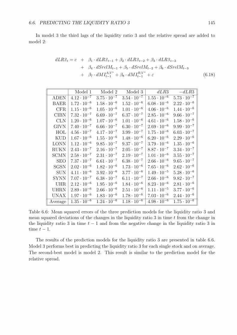
6.6. PREDICTING THE LIQUIDITY RATIO 3 145
In model 3 the third lags of the liquidity ratio 3 and the relative spread are added to
model 2:
dLR3 t = c + β1 · dLR3 t−1 + β2 · dLR3 t−2 + β3 · dLR3 t−3
+ β4 · dSrelMt−1 + β5 · dSrelMt−2 + β6 · dSrelMt−3
+ β7 · dMIA,V ∗t−1 + β8 · dMIB,V ∗
t−1 + ε (6.18)
Model 1 Model 2 Model 3 dLR3 −dLR3ADEN 4.12 · 10−7 3.75 · 10−7 3.54 · 10−7 1.55 · 10−6 5.73 · 10−7
BAER 1.72 · 10−6 1.58 · 10−6 1.52 · 10−6 6.08 · 10−6 2.22 · 10−6
CFR 1.15 · 10−6 1.05 · 10−6 1.01 · 10−6 4.06 · 10−6 1.44 · 10−6
CIBN 7.32 · 10−7 6.69 · 10−7 6.37 · 10−7 2.85 · 10−6 9.66 · 10−7
CLN 1.20 · 10−6 1.07 · 10−6 1.01 · 10−6 4.61 · 10−6 1.58 · 10−6
GIVN 7.40 · 10−7 6.66 · 10−7 6.30 · 10−7 2.69 · 10−6 9.99 · 10−7
HOL 4.56 · 10−7 4.17 · 10−7 3.99 · 10−7 1.75 · 10−6 6.03 · 10−7
KUD 1.67 · 10−6 1.55 · 10−6 1.48 · 10−6 6.20 · 10−6 2.29 · 10−6
LONN 1.12 · 10−6 9.85 · 10−7 9.37 · 10−7 3.79 · 10−6 1.35 · 10−6
RUKN 2.43 · 10−7 2.16 · 10−7 2.05 · 10−7 8.87 · 10−7 3.34 · 10−7
SCMN 2.58 · 10−7 2.31 · 10−7 2.19 · 10−7 1.01 · 10−6 3.55 · 10−7
SEO 7.37 · 10−7 6.61 · 10−7 6.38 · 10−7 2.66 · 10−6 9.65 · 10−7
SGSN 2.02 · 10−6 1.82 · 10−6 1.73 · 10−6 7.65 · 10−6 2.62 · 10−6
SUN 4.11 · 10−6 3.92 · 10−6 3.77 · 10−6 1.49 · 10−5 5.28 · 10−6
SYNN 7.07 · 10−7 6.38 · 10−7 6.11 · 10−7 2.66 · 10−6 9.82 · 10−7
UHR 2.12 · 10−6 1.95 · 10−6 1.84 · 10−6 8.23 · 10−6 2.81 · 10−6
UHRN 2.89 · 10−6 2.66 · 10−6 2.51 · 10−6 1.11 · 10−5 3.77 · 10−6
UNAX 1.97 · 10−6 1.83 · 10−6 1.78 · 10−6 7.03 · 10−6 2.44 · 10−6
Average 1.35 · 10−6 1.24 · 10−6 1.18 · 10−6 4.98 · 10−6 1.75 · 10−6
Table 6.6: Mean squared errors of the three prediction models for the liquidity ratio 3 andmean squared deviations of the changes in the liquidity ratio 3 in time t from the change inthe liquidity ratio 3 in time t − 1 and from the negative change in the liquidity ratio 3 intime t− 1.
The results of the prediction models for the liquidity ratio 3 are presented in table 6.6.
Model 3 performs best in predicting the liquidity ratio 3 for each single stock and on average.
The second-best model is model 2. This result is similar to the prediction model for the
relative spread.

146 CHAPTER 6. PREDICTION MODELS FOR LIQUIDITY
Chapter 7
Summary and Outlook
Liquidity is not a one-dimensional variable. Traditionally, the different dimensions of liquid-
ity in a limit order book are trading time, depth, tightness and resiliency. These dimensions
can be measured by a variety of liquidity measures as current research in this area shows.
31 of them, which are empirically used in the present dissertation, are described in the first
chapter.
Intraday data was collected for a sample of 18 stocks of the Swiss Market Index which
includes 65 trading days. With the order history reports of the Swiss Exchange the recon-
struction of order books is possible. For this sample, the liquidity measures are calculated
on a five-minute interval and compared to each other. Among the 18 stocks, there are huge
differences in liquidity – over time and with respect to the other stocks. The stocks are
ranked according to the different liquidity measures and a clear difference shows up between
the most liquid stock in this study, Swiss Re, and the least liquid, Sulzer. The rankings of
the stocks according to different liquidity measures are tested for their significance using the
Spearman rank correlation test. Two groups of liquidity measures can be distinguished from
this test: One group contains all the liquidity measures that depend on the absolute stock
price, the other group contains the liquidity measures which are independent of the stock
price. Only the order ratio cannot be attributed to one of those groups. For the eighteen
stocks, the correlations of the liquidity measures are calculated – for each stock and on av-
erage. It is apparent that some measures describe the same changes in liquidity. Therefore,
eight liquidity measures are sorted out.
With the remaining 23 liquidity measures, a principal component analysis is carried out
for each stock to investigate how the different dimensions of liquidity can be incorporated
in liquidity measures. Due to the right-skewed and fat-tailed distributional properties, this
principal component analysis is based on the first differences of the liquidity measures. As
it turns out, liquidity cannot be fully described by the above-mentioned four dimensions of
liquidity. As a fifth and a sixth dimension a bid-side and an ask-side related liquidity had to
be introduced. The six dimensions of liquidity are described by the relative spread, turnover,
dollar depth, market impact on the ask-side and market impact on the bid-side.
To investigate the lead-lag patterns of liquidity, a vector autoregressive model is built
with the changes of these six measures and returns. The changes in liquidity show negative
autocorrelations; periods of high liquidity tend to be followed by periods of low liquidity
and vice versa. Rising turnover and rising market impact measures lead to a higher relative
147
148 CHAPTER 7. SUMMARY AND OUTLOOK
spread. A rising relative spread and a rising market impact on the ask-side have a negative
effect on turnover. For the market impact on the bid-side no such effect can be found. An
increase in dollar depth also increases turnover. Also, declining liquidity as measured by
the relative spread leads to a declining depth. A higher turnover is related to rising market
impact on the ask-side and on the bid-side of the limit order book. Lower liquidity on
the ask-side of the order book is followed by lower liquidity on the bid-side. No consistent
influence from the bid-side to the ask-side of the order book can be found across the 18
stocks. A rising relative spread and a rising market impact on the bid-side lead to a higher
liquidity ratio 3. Low liquidity on the ask-side leads to higher stock prices, low liquidity on
the bid-side to lower ones. In general, the impact of returns on liquidity and vice versa is
weak.
Linear prediction models are built for the six liquidity measures mentioned above, based
on lagged liquidity and returns. The models for the relative spread, turnover and the liquidity
ratio 3 show promising results, while the models for the market impact measures and – to a
lesser extent – for dollar depth perform very poorly.
The prediction models of chapter 6 leave room for further research. Advanced models,
using for example a GARCH approach, may lead to more accurate predictions of liquidity.
Another line of research would be the modelling of extreme events. With the data of
stock market crashes it would be interesting to investigate whether the correlations and factor
structures are stable in extreme market situations and whether the prediction of liquidity is
still possible.
Finally, the impact of large orders entered in the order book is only poorly investigated
so far. For decisions on how and when large orders should be placed in the order book, the
development of liquidity in the aftermath of such large order placements may be crucial.
Appendix A
Liquidity Measures Not Used in the
present Dissertation
This appendix describes liquidity measures that are not used in the empirical work.
A.1 Size of the Firm
Usually the liquidity measures related to firm size give a rather crude measure of liquidity,
but they do pretty well in studies that use only monthly instead of higher frequency data.
The following measures may be used:
• Market capitalization
• Free float
In line with the adjustment of the index calculation recently, free float is considered as
the relevant measure. Only the free float part of the market capitalization can be traded at
the exchange and is, therefore, relevant as a measure of market liquidity.
• Number of shareholders
• Number of market makers
In the present dissertation these four proxies for the size of firm are not investigated
further1 because in a context of daily or intradaily measurement they do not show enough
variation. But they may be very useful in cross-sectional studies, as e.g. in Loderer & Roth
(2001) for the Swiss market, that have a focus on the impact of liquidity on stock prices in
the long run.
1Open interest as liquidity proxy for the futures market, which is used in Clyman et al. (1997), is obviouslyneglected in this dissertation.
149
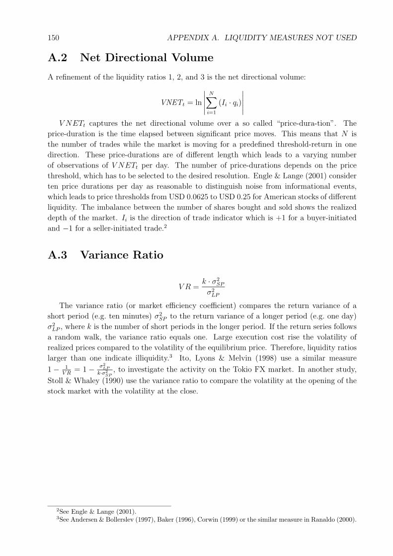
150 APPENDIX A. LIQUIDITY MEASURES NOT USED
A.2 Net Directional Volume
A refinement of the liquidity ratios 1, 2, and 3 is the net directional volume:
VNETt = ln
∣∣∣∣∣N∑
i=1
(Ii · qi)
∣∣∣∣∣V NETt captures the net directional volume over a so called “price-dura-tion”. The
price-duration is the time elapsed between significant price moves. This means that N is
the number of trades while the market is moving for a predefined threshold-return in one
direction. These price-durations are of different length which leads to a varying number
of observations of V NETt per day. The number of price-durations depends on the price
threshold, which has to be selected to the desired resolution. Engle & Lange (2001) consider
ten price durations per day as reasonable to distinguish noise from informational events,
which leads to price thresholds from USD 0.0625 to USD 0.25 for American stocks of different
liquidity. The imbalance between the number of shares bought and sold shows the realized
depth of the market. Ii is the direction of trade indicator which is +1 for a buyer-initiated
and −1 for a seller-initiated trade.2
A.3 Variance Ratio
V R =k · σ2
SP
σ2LP
The variance ratio (or market efficiency coefficient) compares the return variance of a
short period (e.g. ten minutes) σ2SP to the return variance of a longer period (e.g. one day)
σ2LP , where k is the number of short periods in the longer period. If the return series follows
a random walk, the variance ratio equals one. Large execution cost rise the volatility of
realized prices compared to the volatility of the equilibrium price. Therefore, liquidity ratios
larger than one indicate illiquidity.3 Ito, Lyons & Melvin (1998) use a similar measure
1 − 1V R
= 1 − σ2LP
k·σ2SP
, to investigate the activity on the Tokio FX market. In another study,
Stoll & Whaley (1990) use the variance ratio to compare the volatility at the opening of the
stock market with the volatility at the close.
2See Engle & Lange (2001).3See Andersen & Bollerslev (1997), Baker (1996), Corwin (1999) or the similar measure in Ranaldo (2000).
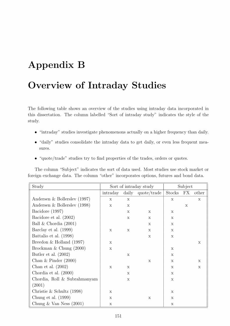
Appendix B
Overview of Intraday Studies
The following table shows an overview of the studies using intraday data incorporated in
this dissertation. The column labelled “Sort of intraday study” indicates the style of the
study.
• “intraday” studies investigate phenomenons actually on a higher frequency than daily.
• “daily” studies consolidate the intraday data to get daily, or even less frequent mea-
sures.
• “quote/trade” studies try to find properties of the trades, orders or quotes.
The column “Subject” indicates the sort of data used. Most studies use stock market or
foreign exchange data. The column “other” incorporates options, futures and bond data.
Study Sort of intraday study Subject
intraday daily quote/trade Stocks FX other
Andersen & Bollerslev (1997) x x x x
Andersen & Bollerslev (1998) x x x
Bacidore (1997) x x x
Bacidore et al. (2002) x x x
Ball & Chordia (2001) x x
Barclay et al. (1999) x x x x
Battalio et al. (1998) x x
Breedon & Holland (1997) x x
Brockman & Chung (2000) x x
Butler et al. (2002) x x
Chan & Pinder (2000) x x x
Chan et al. (2002) x x x x
Chordia et al. (2000) x x
Chordia, Roll & Subrahmanyam
(2001)
x x
Christie & Schultz (1998) x x
Chung et al. (1999) x x x
Chung & Van Ness (2001) x x
151
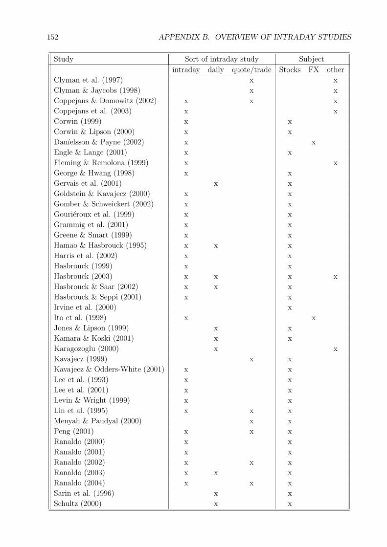
152 APPENDIX B. OVERVIEW OF INTRADAY STUDIES
Study Sort of intraday study Subject
intraday daily quote/trade Stocks FX other
Clyman et al. (1997) x x
Clyman & Jaycobs (1998) x x
Coppejans & Domowitz (2002) x x x
Coppejans et al. (2003) x x
Corwin (1999) x x
Corwin & Lipson (2000) x x
Danıelsson & Payne (2002) x x
Engle & Lange (2001) x x
Fleming & Remolona (1999) x x
George & Hwang (1998) x x
Gervais et al. (2001) x x
Goldstein & Kavajecz (2000) x x
Gomber & Schweickert (2002) x x
Gourieroux et al. (1999) x x
Grammig et al. (2001) x x
Greene & Smart (1999) x x
Hamao & Hasbrouck (1995) x x x
Harris et al. (2002) x x
Hasbrouck (1999) x x
Hasbrouck (2003) x x x x
Hasbrouck & Saar (2002) x x x
Hasbrouck & Seppi (2001) x x
Irvine et al. (2000) x
Ito et al. (1998) x x
Jones & Lipson (1999) x x
Kamara & Koski (2001) x x
Karagozoglu (2000) x x
Kavajecz (1999) x x
Kavajecz & Odders-White (2001) x x
Lee et al. (1993) x x
Lee et al. (2001) x x
Levin & Wright (1999) x x
Lin et al. (1995) x x x
Menyah & Paudyal (2000) x x
Peng (2001) x x x
Ranaldo (2000) x x
Ranaldo (2001) x x
Ranaldo (2002) x x x
Ranaldo (2003) x x x
Ranaldo (2004) x x x
Sarin et al. (1996) x x
Schultz (2000) x x
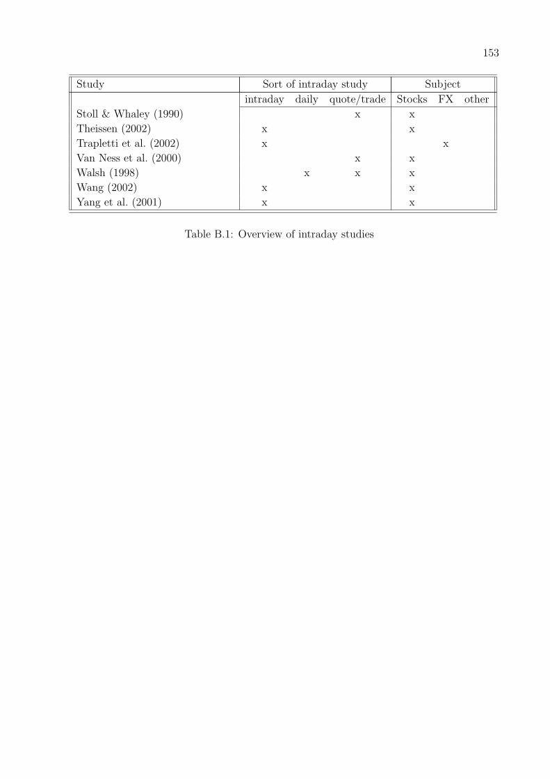
153
Study Sort of intraday study Subject
intraday daily quote/trade Stocks FX other
Stoll & Whaley (1990) x x
Theissen (2002) x x
Trapletti et al. (2002) x x
Van Ness et al. (2000) x x
Walsh (1998) x x x
Wang (2002) x x
Yang et al. (2001) x x
Table B.1: Overview of intraday studies

154 APPENDIX B. OVERVIEW OF INTRADAY STUDIES
Appendix C
Correlation Matrices of the 31
Liquidity Measures for the 18 Stocks
155

156 APPENDIX C. CORRELATION MATRICES
Q V D Dlog D$ N NO Sabs LogSabs SrelM SrelpQ 1V 0.98 1D 0.05 0.05 1
Dlog -0.02 0.02 0.28 1D$ 0.03 0.05 1.00 0.32 1N 0.83 0.81 0.01 -0.11 0.00 1
NO 0.67 0.64 0.01 -0.17 -0.02 0.80 1Sabs 0.03 0.04 0.09 0.35 0.11 -0.01 -0.01 1
LogSabs 0.00 0.01 0.09 0.37 0.12 -0.04 -0.04 0.92 1SrelM 0.08 0.05 0.05 0.21 0.05 0.05 0.08 0.94 0.85 1Srelp 0.08 0.05 0.05 0.21 0.05 0.05 0.08 0.94 0.85 1.00 1
Srellog 0.08 0.05 0.05 0.21 0.05 0.05 0.08 0.94 0.85 1.00 1.00LogSrellog 0.03 0.02 0.07 0.28 0.08 0.00 0.03 0.90 0.97 0.89 0.89
Seff -0.02 -0.02 0.08 0.24 0.10 -0.04 -0.03 0.61 0.61 0.58 0.58Seffrelp 0.03 0.00 0.05 0.12 0.05 0.01 0.05 0.58 0.56 0.64 0.64
SeffrelM 0.03 0.00 0.05 0.12 0.05 0.01 0.05 0.58 0.56 0.64 0.64QS 0.05 0.04 0.02 0.09 0.03 0.03 0.05 0.95 0.88 0.95 0.95
LogQS 0.09 0.05 -0.01 -0.04 -0.02 0.08 0.13 0.86 0.77 0.96 0.96LogQSadj 0.11 0.07 0.00 -0.23 -0.01 0.11 0.13 0.54 0.47 0.65 0.65
CL 0.06 0.02 -0.09 -0.44 -0.10 0.09 0.13 0.17 0.15 0.29 0.29LR1 0.51 0.52 0.00 -0.04 0.00 0.40 0.29 -0.14 -0.15 -0.12 -0.12LR3 0.02 -0.01 0.01 0.02 0.01 -0.02 0.10 0.28 0.27 0.35 0.35FR 0.79 0.81 0.03 0.00 0.03 0.69 0.50 0.00 -0.02 0.02 0.02OR -0.07 -0.07 0.04 0.08 0.05 -0.09 -0.08 0.03 0.04 0.01 0.01
MIV ∗ 0.03 -0.02 -0.12 -0.35 -0.14 0.08 0.15 0.25 0.21 0.38 0.38
MIA,V ∗ 0.02 -0.03 -0.09 -0.29 -0.11 0.06 0.13 0.19 0.16 0.30 0.30
MIB,V ∗ 0.03 -0.01 -0.10 -0.29 -0.12 0.07 0.12 0.22 0.18 0.33 0.33DIA(k) 0.01 0.07 0.12 0.34 0.16 -0.03 -0.11 0.04 0.06 -0.10 -0.10DIB(k) 0.02 0.05 0.63 0.21 0.64 -0.01 -0.07 -0.06 -0.05 -0.13 -0.13PIA(q) 0.03 -0.02 -0.10 -0.32 -0.12 0.08 0.15 0.23 0.19 0.37 0.37PIB(q) 0.05 -0.01 -0.11 -0.31 -0.13 0.09 0.14 0.26 0.21 0.39 0.39
Srellog LogSrellog Seff Seffrelp SeffrelM QS LogQS LogQSadj CL LR1 LR3Srellog 1
LogSrellog 0.89 1Seff 0.58 0.59 1
Seffrelp 0.64 0.59 0.95 1SeffrelM 0.64 0.59 0.95 1.00 1
QS 0.95 0.89 0.59 0.60 0.60 1LogQS 0.96 0.84 0.54 0.63 0.63 0.95 1
LogQSadj 0.65 0.54 0.37 0.46 0.46 0.68 0.76 1CL 0.29 0.22 0.12 0.22 0.22 0.37 0.48 0.32 1
LR1 -0.12 -0.15 -0.15 -0.13 -0.13 -0.13 -0.11 -0.06 -0.03 1LR3 0.35 0.32 0.28 0.33 0.33 0.30 0.35 0.24 0.15 -0.10 1FR 0.02 -0.01 -0.02 0.00 0.00 0.01 0.02 0.04 0.02 0.32 0.01OR 0.01 0.03 0.05 0.03 0.03 0.01 -0.01 0.00 -0.03 -0.05 0.12
MIV ∗ 0.38 0.31 0.18 0.30 0.30 0.38 0.48 0.38 0.37 -0.12 0.26
MIA,V ∗ 0.30 0.25 0.13 0.23 0.23 0.29 0.39 0.30 0.30 -0.10 0.21
MIB,V ∗ 0.33 0.27 0.17 0.27 0.27 0.32 0.41 0.33 0.30 -0.10 0.22DIA(k) -0.10 -0.05 0.03 -0.09 -0.09 -0.06 -0.19 -0.16 -0.21 0.08 -0.12DIB(k) -0.13 -0.11 -0.03 -0.09 -0.09 -0.12 -0.18 -0.12 -0.14 0.07 -0.11PIA(q) 0.37 0.29 0.16 0.28 0.28 0.35 0.47 0.38 0.36 -0.10 0.25PIB(q) 0.39 0.31 0.20 0.32 0.32 0.37 0.48 0.39 0.36 -0.10 0.25
FR OR MIV ∗ MIA,V ∗ MIB,V ∗ DIA(k) DIB(k) PIA(q) PIB(q)FR 1OR -0.03 1
MIV ∗ -0.01 -0.04 1
MIA,V ∗ -0.02 -0.02 0.83 1
MIB,V ∗ 0.00 -0.04 0.81 0.35 1DIA(k) 0.03 0.04 -0.46 -0.46 -0.28 1DIB(k) 0.02 0.02 -0.33 -0.22 -0.33 0.20 1PIA(q) -0.01 -0.03 0.82 0.95 0.38 -0.50 -0.23 1PIB(q) 0.01 -0.04 0.81 0.39 0.95 -0.31 -0.35 0.44 1
Table C.1: Correlation matrix of the 31 liquidity measures for Adecco

157
Q V D Dlog D$ N NO Sabs LogSabs SrelM SrelpQ 1V 0.99 1D -0.06 -0.01 1
Dlog -0.02 0.02 0.74 1D$ -0.06 -0.01 0.99 0.68 1N 0.70 0.69 -0.16 -0.10 -0.17 1
NO 0.42 0.41 -0.18 -0.14 -0.18 0.62 1Sabs 0.05 0.03 -0.18 -0.19 -0.17 0.08 0.22 1
LogSabs 0.04 0.02 -0.16 -0.18 -0.15 0.06 0.18 0.93 1SrelM 0.07 0.04 -0.30 -0.27 -0.29 0.11 0.24 0.98 0.90 1Srelp 0.07 0.04 -0.30 -0.27 -0.29 0.11 0.24 0.98 0.90 1.00 1
Srellog 0.07 0.04 -0.30 -0.27 -0.29 0.11 0.24 0.98 0.90 1.00 1.00LogSrellog 0.05 0.03 -0.31 -0.27 -0.30 0.10 0.22 0.92 0.98 0.92 0.92
Seff 0.06 0.04 -0.21 -0.24 -0.19 0.07 0.19 0.85 0.80 0.83 0.83Seffrelp 0.07 0.04 -0.30 -0.29 -0.29 0.10 0.20 0.79 0.73 0.81 0.81
SeffrelM 0.07 0.04 -0.30 -0.29 -0.29 0.10 0.21 0.80 0.74 0.81 0.82QS 0.06 0.03 -0.37 -0.46 -0.33 0.10 0.23 0.92 0.85 0.94 0.94
LogQS 0.07 0.03 -0.45 -0.51 -0.42 0.12 0.25 0.88 0.80 0.93 0.93LogQSadj 0.03 0.01 -0.19 -0.30 -0.20 0.09 0.21 0.84 0.79 0.84 0.84
CL 0.05 0.02 -0.40 -0.56 -0.34 0.07 0.12 0.28 0.24 0.35 0.35LR1 0.71 0.72 0.03 0.05 0.03 0.46 0.22 -0.04 -0.05 -0.04 -0.04LR3 0.07 0.05 -0.20 -0.17 -0.21 0.10 0.24 0.24 0.21 0.27 0.27FR 0.84 0.84 -0.02 0.00 -0.02 0.65 0.39 0.04 0.04 0.05 0.05OR -0.10 -0.10 0.08 0.05 0.08 -0.12 -0.08 0.00 0.01 -0.01 -0.01
MIV ∗ 0.03 0.00 -0.42 -0.47 -0.38 0.11 0.16 0.22 0.21 0.28 0.28
MIA,V ∗ 0.05 0.01 -0.43 -0.50 -0.38 0.13 0.17 0.26 0.24 0.33 0.33
MIB,V ∗ 0.02 0.00 -0.34 -0.37 -0.31 0.08 0.13 0.17 0.16 0.21 0.21DIA(k) -0.06 0.00 0.91 0.60 0.92 -0.18 -0.20 -0.20 -0.19 -0.33 -0.33DIB(k) 0.04 0.04 0.32 0.26 0.29 0.00 -0.01 -0.04 -0.06 -0.02 -0.02PIA(q) 0.04 0.00 -0.50 -0.57 -0.43 0.08 0.12 0.18 0.17 0.24 0.24PIB(q) 0.02 -0.01 -0.67 -0.68 -0.59 0.09 0.11 0.21 0.20 0.29 0.29
Srellog LogSrellog Seff Seffrelp SeffrelM QS LogQS LogQSadj CL LR1 LR3Srellog 1
LogSrellog 0.92 1Seff 0.83 0.80 1
Seffrelp 0.81 0.75 0.98 1SeffrelM 0.81 0.76 0.98 1.00 1
QS 0.94 0.87 0.80 0.77 0.78 1LogQS 0.93 0.84 0.76 0.76 0.77 0.99 1
LogQSadj 0.84 0.80 0.71 0.68 0.68 0.79 0.76 1CL 0.35 0.28 0.27 0.32 0.32 0.58 0.62 0.19 1
LR1 -0.04 -0.06 -0.04 -0.04 -0.04 -0.04 -0.04 -0.06 0.00 1LR3 0.27 0.25 0.22 0.23 0.24 0.27 0.28 0.22 0.15 0.00 1FR 0.05 0.04 0.04 0.05 0.05 0.04 0.04 0.03 0.01 0.57 0.03OR -0.01 0.00 0.00 -0.01 -0.01 -0.02 -0.03 0.01 -0.04 -0.08 0.09
MIV ∗ 0.28 0.27 0.17 0.21 0.22 0.36 0.40 0.20 0.36 -0.05 0.16
MIA,V ∗ 0.33 0.30 0.21 0.26 0.26 0.41 0.47 0.19 0.46 -0.03 0.16
MIB,V ∗ 0.21 0.21 0.13 0.16 0.16 0.27 0.30 0.16 0.25 -0.05 0.12DIA(k) -0.33 -0.34 -0.17 -0.27 -0.27 -0.35 -0.43 -0.24 -0.32 0.05 -0.23DIB(k) -0.02 -0.07 -0.01 0.01 0.01 -0.09 -0.08 -0.04 -0.08 0.03 -0.02PIA(q) 0.24 0.24 0.12 0.17 0.17 0.36 0.41 0.09 0.45 -0.02 0.13PIB(q) 0.29 0.29 0.13 0.19 0.19 0.41 0.47 0.12 0.47 -0.04 0.15
FR OR MIV ∗ MIA,V ∗ MIB,V ∗ DIA(k) DIB(k) PIA(q) PIB(q)FR 1OR -0.05 1
MIV ∗ 0.02 -0.04 1
MIA,V ∗ 0.02 -0.04 0.50 1
MIB,V ∗ 0.01 -0.03 0.96 0.25 1DIA(k) -0.02 0.07 -0.40 -0.47 -0.30 1DIB(k) 0.03 0.02 -0.23 0.01 -0.26 0.22 1PIA(q) 0.01 -0.05 0.48 0.79 0.29 -0.52 -0.11 1PIB(q) 0.00 -0.06 0.68 0.57 0.58 -0.63 -0.36 0.74 1
Table C.2: Correlation matrix of the 31 liquidity measures for Baer

158 APPENDIX C. CORRELATION MATRICES
Q V D Dlog D$ N NO Sabs LogSabs SrelM SrelpQ 1V 0.99 1D 0.03 0.04 1
Dlog 0.00 0.01 0.75 1D$ 0.02 0.04 0.99 0.72 1N 0.70 0.69 -0.04 -0.07 -0.06 1
NO 0.60 0.57 -0.05 -0.07 -0.08 0.80 1Sabs 0.12 0.11 -0.03 -0.02 -0.05 0.16 0.25 1
LogSabs 0.13 0.11 -0.03 0.00 -0.05 0.16 0.24 0.90 1SrelM 0.13 0.10 -0.04 -0.03 -0.08 0.18 0.28 0.98 0.88 1Srelp 0.14 0.10 -0.04 -0.03 -0.08 0.18 0.28 0.98 0.88 1.00 1
Srellog 0.13 0.10 -0.04 -0.03 -0.08 0.18 0.28 0.98 0.88 1.00 1.00LogSrellog 0.14 0.10 -0.05 -0.02 -0.10 0.18 0.28 0.87 0.97 0.90 0.90
Seff 0.04 0.03 -0.07 -0.09 -0.08 0.09 0.21 0.64 0.51 0.63 0.63Seffrelp 0.05 0.03 -0.07 -0.10 -0.10 0.11 0.24 0.64 0.51 0.65 0.65
SeffrelM 0.05 0.03 -0.07 -0.10 -0.10 0.11 0.24 0.64 0.51 0.66 0.66QS 0.12 0.10 -0.12 -0.17 -0.13 0.16 0.25 0.97 0.85 0.95 0.95
LogQS 0.13 0.10 -0.13 -0.18 -0.16 0.18 0.28 0.96 0.84 0.98 0.98LogQSadj 0.09 0.06 -0.09 -0.32 -0.12 0.15 0.22 0.75 0.63 0.76 0.76
CL 0.06 0.04 -0.17 -0.31 -0.16 0.08 0.12 0.36 0.24 0.37 0.37LR1 0.58 0.62 0.04 0.02 0.05 0.47 0.33 -0.01 0.01 -0.03 -0.03LR3 -0.01 -0.03 -0.08 -0.10 -0.11 -0.01 0.15 0.29 0.28 0.32 0.32FR 0.88 0.88 0.00 -0.02 0.00 0.53 0.47 0.10 0.09 0.10 0.10OR -0.07 -0.07 0.05 0.03 0.05 -0.09 -0.07 -0.01 -0.01 -0.01 -0.01
MIV ∗ 0.02 0.00 -0.13 -0.15 -0.14 0.07 0.08 0.13 0.13 0.18 0.18
MIA,V ∗ 0.04 0.00 -0.24 -0.28 -0.26 0.11 0.16 0.26 0.24 0.32 0.32
MIB,V ∗ 0.01 0.00 -0.08 -0.10 -0.09 0.04 0.05 0.08 0.09 0.11 0.11DIA(k) 0.01 0.06 0.27 0.22 0.33 -0.07 -0.16 -0.21 -0.23 -0.27 -0.27DIB(k) 0.04 0.07 0.27 0.23 0.30 -0.02 -0.08 -0.18 -0.18 -0.21 -0.21PIA(q) 0.06 0.02 -0.28 -0.36 -0.29 0.15 0.22 0.45 0.39 0.49 0.49PIB(q) 0.01 0.00 -0.09 -0.13 -0.09 0.05 0.07 0.13 0.13 0.16 0.16
Srellog LogSrellog Seff Seffrelp SeffrelM QS LogQS LogQSadj CL LR1 LR3Srellog 1
LogSrellog 0.90 1Seff 0.63 0.50 1
Seffrelp 0.65 0.54 0.98 1SeffrelM 0.66 0.54 0.99 1.00 1
QS 0.95 0.83 0.65 0.64 0.64 1LogQS 0.98 0.85 0.64 0.66 0.66 0.98 1
LogQSadj 0.76 0.64 0.53 0.54 0.54 0.81 0.82 1CL 0.37 0.26 0.29 0.30 0.30 0.52 0.52 0.36 1
LR1 -0.03 -0.02 -0.06 -0.08 -0.08 -0.01 -0.03 -0.02 -0.01 1LR3 0.32 0.31 0.30 0.32 0.32 0.30 0.33 0.36 0.09 -0.07 1FR 0.10 0.09 0.04 0.05 0.05 0.10 0.10 0.07 0.05 0.41 -0.01OR -0.01 -0.01 0.01 0.00 0.00 -0.01 -0.02 0.00 -0.02 -0.06 0.04
MIV ∗ 0.18 0.18 0.12 0.16 0.16 0.15 0.19 0.16 0.11 -0.04 0.11
MIA,V ∗ 0.32 0.31 0.20 0.25 0.25 0.29 0.35 0.27 0.21 -0.07 0.17
MIB,V ∗ 0.11 0.12 0.09 0.11 0.11 0.09 0.12 0.11 0.06 -0.03 0.07DIA(k) -0.27 -0.33 -0.19 -0.23 -0.23 -0.23 -0.29 -0.22 -0.14 0.14 -0.19DIB(k) -0.21 -0.24 -0.15 -0.18 -0.18 -0.20 -0.23 -0.19 -0.11 0.12 -0.14PIA(q) 0.49 0.45 0.32 0.37 0.37 0.50 0.54 0.45 0.33 -0.06 0.21PIB(q) 0.16 0.15 0.12 0.14 0.14 0.15 0.18 0.17 0.11 -0.03 0.08
FR OR MIV ∗ MIA,V ∗ MIB,V ∗ DIA(k) DIB(k) PIA(q) PIB(q)FR 1OR -0.03 1
MIV ∗ 0.01 -0.01 1
MIA,V ∗ 0.01 -0.03 0.28 1
MIB,V ∗ 0.00 -0.01 0.98 0.08 1DIA(k) 0.02 0.01 -0.14 -0.38 -0.06 1DIB(k) 0.03 0.00 -0.19 -0.18 -0.15 0.17 1PIA(q) 0.04 -0.03 0.28 0.79 0.12 -0.37 -0.21 1PIB(q) 0.01 0.00 0.45 0.17 0.43 -0.09 -0.13 0.20 1
Table C.3: Correlation matrix of the 31 liquidity measures for Richemont

159
Q V D Dlog D$ N NO Sabs LogSabs SrelM SrelpQ 1V 1.00 1D -0.06 -0.04 1
Dlog -0.12 -0.09 0.79 1D$ -0.07 -0.05 1.00 0.79 1N 0.76 0.74 -0.15 -0.23 -0.16 1
NO 0.63 0.60 -0.19 -0.28 -0.20 0.84 1Sabs 0.11 0.10 0.02 0.10 0.01 0.13 0.17 1
LogSabs 0.07 0.07 0.05 0.16 0.04 0.06 0.09 0.95 1SrelM 0.15 0.13 -0.05 0.01 -0.07 0.19 0.25 0.98 0.92 1Srelp 0.15 0.13 -0.05 0.01 -0.07 0.19 0.25 0.98 0.92 1.00 1
Srellog 0.15 0.13 -0.05 0.01 -0.07 0.19 0.25 0.98 0.92 1.00 1.00LogSrellog 0.12 0.11 -0.03 0.06 -0.05 0.14 0.19 0.95 0.98 0.95 0.95
Seff 0.01 0.00 -0.06 -0.07 -0.06 0.03 0.09 0.21 0.21 0.22 0.22Seffrelp 0.04 0.03 -0.11 -0.13 -0.12 0.08 0.15 0.23 0.22 0.26 0.26
SeffrelM 0.04 0.03 -0.11 -0.13 -0.12 0.08 0.15 0.23 0.22 0.26 0.26QS 0.15 0.13 -0.22 -0.24 -0.23 0.20 0.27 0.93 0.86 0.94 0.94
LogQS 0.18 0.16 -0.26 -0.30 -0.27 0.25 0.34 0.88 0.81 0.93 0.93LogQSadj 0.13 0.12 -0.21 -0.50 -0.21 0.20 0.24 0.38 0.34 0.43 0.43
CL 0.16 0.13 -0.35 -0.55 -0.35 0.25 0.31 0.20 0.15 0.29 0.29LR1 0.66 0.65 -0.07 -0.12 -0.08 0.53 0.44 0.03 -0.02 0.06 0.06LR3 -0.03 -0.03 -0.03 -0.05 -0.03 -0.02 0.07 0.13 0.12 0.15 0.15FR 0.85 0.84 -0.05 -0.08 -0.05 0.66 0.55 0.08 0.05 0.11 0.11OR -0.08 -0.08 0.10 0.06 0.10 -0.10 -0.08 -0.02 -0.01 -0.03 -0.03
MIV ∗ 0.15 0.12 -0.52 -0.60 -0.53 0.28 0.40 0.30 0.22 0.40 0.40
MIA,V ∗ 0.12 0.09 -0.42 -0.48 -0.43 0.22 0.31 0.23 0.17 0.31 0.31
MIB,V ∗ 0.12 0.09 -0.42 -0.48 -0.42 0.23 0.33 0.25 0.19 0.33 0.33DIA(k) -0.14 -0.11 0.57 0.48 0.60 -0.21 -0.27 -0.23 -0.20 -0.33 -0.33DIB(k) -0.08 -0.05 0.58 0.54 0.59 -0.17 -0.28 -0.17 -0.11 -0.26 -0.26PIA(q) 0.14 0.11 -0.46 -0.52 -0.47 0.26 0.35 0.26 0.19 0.36 0.36PIB(q) 0.14 0.11 -0.45 -0.52 -0.46 0.26 0.38 0.28 0.21 0.37 0.37
Srellog LogSrellog Seff Seffrelp SeffrelM QS LogQS LogQSadj CL LR1 LR3Srellog 1
LogSrellog 0.95 1Seff 0.22 0.21 1
Seffrelp 0.26 0.25 0.99 1SeffrelM 0.26 0.25 0.99 1.00 1
QS 0.94 0.90 0.25 0.29 0.29 1LogQS 0.93 0.88 0.24 0.31 0.31 0.98 1
LogQSadj 0.43 0.39 0.16 0.20 0.20 0.61 0.63 1CL 0.29 0.24 0.13 0.20 0.20 0.44 0.51 0.32 1
LR1 0.06 0.02 -0.03 -0.01 -0.01 0.06 0.09 0.08 0.12 1LR3 0.15 0.14 0.14 0.15 0.15 0.15 0.16 0.08 0.07 -0.01 1FR 0.11 0.08 0.03 0.05 0.05 0.11 0.13 0.09 0.14 0.52 -0.02OR -0.03 -0.02 0.01 0.00 0.00 -0.04 -0.04 0.00 -0.04 -0.06 0.10
MIV ∗ 0.40 0.35 0.18 0.26 0.26 0.50 0.57 0.38 0.51 0.11 0.13
MIA,V ∗ 0.31 0.27 0.13 0.20 0.20 0.40 0.46 0.32 0.42 0.08 0.10
MIB,V ∗ 0.33 0.29 0.15 0.22 0.22 0.40 0.46 0.29 0.40 0.09 0.11DIA(k) -0.33 -0.33 -0.10 -0.18 -0.18 -0.36 -0.43 -0.25 -0.31 -0.09 -0.11DIB(k) -0.26 -0.22 -0.08 -0.15 -0.15 -0.33 -0.39 -0.24 -0.36 -0.08 -0.07PIA(q) 0.36 0.31 0.12 0.21 0.21 0.44 0.51 0.35 0.46 0.10 0.12PIB(q) 0.37 0.33 0.16 0.24 0.24 0.45 0.51 0.33 0.45 0.11 0.13
FR OR MIV ∗ MIA,V ∗ MIB,V ∗ DIA(k) DIB(k) PIA(q) PIB(q)FR 1OR -0.04 1
MIV ∗ 0.10 -0.06 1
MIA,V ∗ 0.08 -0.05 0.83 1
MIB,V ∗ 0.09 -0.04 0.77 0.29 1DIA(k) -0.09 0.06 -0.56 -0.53 -0.36 1DIB(k) -0.05 0.04 -0.59 -0.42 -0.54 0.56 1PIA(q) 0.10 -0.06 0.82 0.93 0.35 -0.61 -0.48 1PIB(q) 0.11 -0.05 0.76 0.34 0.92 -0.42 -0.62 0.41 1
Table C.4: Correlation matrix of the 31 liquidity measures for Ciba
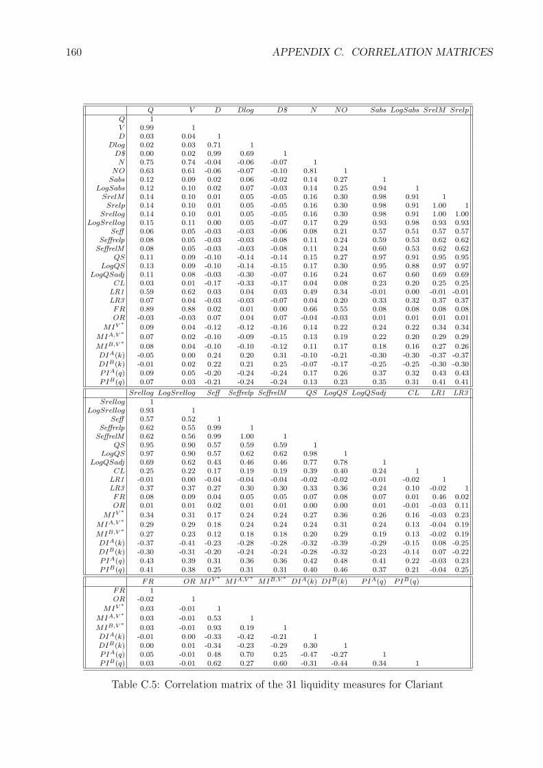
160 APPENDIX C. CORRELATION MATRICES
Q V D Dlog D$ N NO Sabs LogSabs SrelM SrelpQ 1V 0.99 1D 0.03 0.04 1
Dlog 0.02 0.03 0.71 1D$ 0.00 0.02 0.99 0.69 1N 0.75 0.74 -0.04 -0.06 -0.07 1
NO 0.63 0.61 -0.06 -0.07 -0.10 0.81 1Sabs 0.12 0.09 0.02 0.06 -0.02 0.14 0.27 1
LogSabs 0.12 0.10 0.02 0.07 -0.03 0.14 0.25 0.94 1SrelM 0.14 0.10 0.01 0.05 -0.05 0.16 0.30 0.98 0.91 1Srelp 0.14 0.10 0.01 0.05 -0.05 0.16 0.30 0.98 0.91 1.00 1
Srellog 0.14 0.10 0.01 0.05 -0.05 0.16 0.30 0.98 0.91 1.00 1.00LogSrellog 0.15 0.11 0.00 0.05 -0.07 0.17 0.29 0.93 0.98 0.93 0.93
Seff 0.06 0.05 -0.03 -0.03 -0.06 0.08 0.21 0.57 0.51 0.57 0.57Seffrelp 0.08 0.05 -0.03 -0.03 -0.08 0.11 0.24 0.59 0.53 0.62 0.62
SeffrelM 0.08 0.05 -0.03 -0.03 -0.08 0.11 0.24 0.60 0.53 0.62 0.62QS 0.11 0.09 -0.10 -0.14 -0.14 0.15 0.27 0.97 0.91 0.95 0.95
LogQS 0.13 0.09 -0.10 -0.14 -0.15 0.17 0.30 0.95 0.88 0.97 0.97LogQSadj 0.11 0.08 -0.03 -0.30 -0.07 0.16 0.24 0.67 0.60 0.69 0.69
CL 0.03 0.01 -0.17 -0.33 -0.17 0.04 0.08 0.23 0.20 0.25 0.25LR1 0.59 0.62 0.03 0.04 0.03 0.49 0.34 -0.01 0.00 -0.01 -0.01LR3 0.07 0.04 -0.03 -0.03 -0.07 0.04 0.20 0.33 0.32 0.37 0.37FR 0.89 0.88 0.02 0.01 0.00 0.66 0.55 0.08 0.08 0.08 0.08OR -0.03 -0.03 0.07 0.04 0.07 -0.04 -0.03 0.01 0.01 0.01 0.01
MIV ∗ 0.09 0.04 -0.12 -0.12 -0.16 0.14 0.22 0.24 0.22 0.34 0.34
MIA,V ∗ 0.07 0.02 -0.10 -0.09 -0.15 0.13 0.19 0.22 0.20 0.29 0.29
MIB,V ∗ 0.08 0.04 -0.10 -0.10 -0.12 0.11 0.17 0.18 0.16 0.27 0.26DIA(k) -0.05 0.00 0.24 0.20 0.31 -0.10 -0.21 -0.30 -0.30 -0.37 -0.37DIB(k) -0.01 0.02 0.22 0.21 0.25 -0.07 -0.17 -0.25 -0.25 -0.30 -0.30PIA(q) 0.09 0.05 -0.20 -0.24 -0.24 0.17 0.26 0.37 0.32 0.43 0.43PIB(q) 0.07 0.03 -0.21 -0.24 -0.24 0.13 0.23 0.35 0.31 0.41 0.41
Srellog LogSrellog Seff Seffrelp SeffrelM QS LogQS LogQSadj CL LR1 LR3Srellog 1
LogSrellog 0.93 1Seff 0.57 0.52 1
Seffrelp 0.62 0.55 0.99 1SeffrelM 0.62 0.56 0.99 1.00 1
QS 0.95 0.90 0.57 0.59 0.59 1LogQS 0.97 0.90 0.57 0.62 0.62 0.98 1
LogQSadj 0.69 0.62 0.43 0.46 0.46 0.77 0.78 1CL 0.25 0.22 0.17 0.19 0.19 0.39 0.40 0.24 1
LR1 -0.01 0.00 -0.04 -0.04 -0.04 -0.02 -0.02 -0.01 -0.02 1LR3 0.37 0.37 0.27 0.30 0.30 0.33 0.36 0.24 0.10 -0.02 1FR 0.08 0.09 0.04 0.05 0.05 0.07 0.08 0.07 0.01 0.46 0.02OR 0.01 0.01 0.02 0.01 0.01 0.00 0.00 0.01 -0.01 -0.03 0.11
MIV ∗ 0.34 0.31 0.17 0.24 0.24 0.27 0.36 0.26 0.16 -0.03 0.23
MIA,V ∗ 0.29 0.29 0.18 0.24 0.24 0.24 0.31 0.24 0.13 -0.04 0.19
MIB,V ∗ 0.27 0.23 0.12 0.18 0.18 0.20 0.29 0.19 0.13 -0.02 0.19DIA(k) -0.37 -0.41 -0.23 -0.28 -0.28 -0.32 -0.39 -0.29 -0.15 0.08 -0.25DIB(k) -0.30 -0.31 -0.20 -0.24 -0.24 -0.28 -0.32 -0.23 -0.14 0.07 -0.22PIA(q) 0.43 0.39 0.31 0.36 0.36 0.42 0.48 0.41 0.22 -0.03 0.23PIB(q) 0.41 0.38 0.25 0.31 0.31 0.40 0.46 0.37 0.21 -0.04 0.25
FR OR MIV ∗ MIA,V ∗ MIB,V ∗ DIA(k) DIB(k) PIA(q) PIB(q)FR 1OR -0.02 1
MIV ∗ 0.03 -0.01 1
MIA,V ∗ 0.03 -0.01 0.53 1
MIB,V ∗ 0.03 -0.01 0.93 0.19 1DIA(k) -0.01 0.00 -0.33 -0.42 -0.21 1DIB(k) 0.00 0.01 -0.34 -0.23 -0.29 0.30 1PIA(q) 0.05 -0.01 0.48 0.70 0.25 -0.47 -0.27 1PIB(q) 0.03 -0.01 0.62 0.27 0.60 -0.31 -0.44 0.34 1
Table C.5: Correlation matrix of the 31 liquidity measures for Clariant
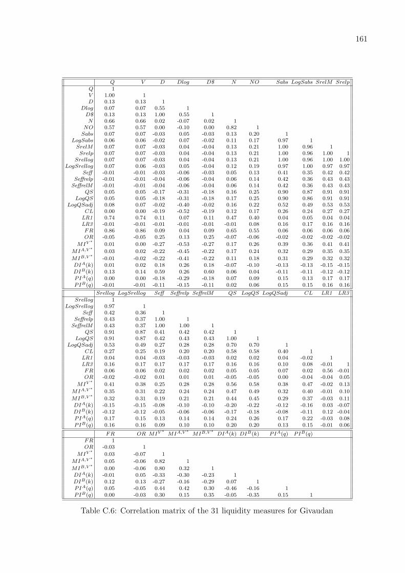
161
Q V D Dlog D$ N NO Sabs LogSabs SrelM SrelpQ 1V 1.00 1D 0.13 0.13 1
Dlog 0.07 0.07 0.55 1D$ 0.13 0.13 1.00 0.55 1N 0.66 0.66 0.02 -0.07 0.02 1
NO 0.57 0.57 0.00 -0.10 0.00 0.82 1Sabs 0.07 0.07 -0.03 0.05 -0.03 0.13 0.20 1
LogSabs 0.06 0.06 -0.02 0.07 -0.02 0.11 0.17 0.97 1SrelM 0.07 0.07 -0.03 0.04 -0.04 0.13 0.21 1.00 0.96 1Srelp 0.07 0.07 -0.03 0.04 -0.04 0.13 0.21 1.00 0.96 1.00 1
Srellog 0.07 0.07 -0.03 0.04 -0.04 0.13 0.21 1.00 0.96 1.00 1.00LogSrellog 0.07 0.06 -0.03 0.05 -0.04 0.12 0.19 0.97 1.00 0.97 0.97
Seff -0.01 -0.01 -0.03 -0.06 -0.03 0.05 0.13 0.41 0.35 0.42 0.42Seffrelp -0.01 -0.01 -0.04 -0.06 -0.04 0.06 0.14 0.42 0.36 0.43 0.43
SeffrelM -0.01 -0.01 -0.04 -0.06 -0.04 0.06 0.14 0.42 0.36 0.43 0.43QS 0.05 0.05 -0.17 -0.31 -0.18 0.16 0.25 0.90 0.87 0.91 0.91
LogQS 0.05 0.05 -0.18 -0.31 -0.18 0.17 0.25 0.90 0.86 0.91 0.91LogQSadj 0.08 0.07 -0.02 -0.40 -0.02 0.16 0.22 0.52 0.49 0.53 0.53
CL 0.00 0.00 -0.19 -0.52 -0.19 0.12 0.17 0.26 0.24 0.27 0.27LR1 0.74 0.74 0.11 0.07 0.11 0.47 0.40 0.04 0.05 0.04 0.04LR3 -0.01 -0.01 -0.01 -0.01 -0.01 -0.01 0.08 0.16 0.17 0.16 0.16FR 0.86 0.86 0.09 0.04 0.09 0.65 0.55 0.06 0.06 0.06 0.06OR -0.05 -0.05 0.25 0.13 0.25 -0.07 -0.06 -0.02 -0.02 -0.02 -0.02
MIV ∗ 0.01 0.00 -0.27 -0.53 -0.27 0.17 0.26 0.39 0.36 0.41 0.41
MIA,V ∗ 0.03 0.02 -0.22 -0.45 -0.22 0.17 0.24 0.32 0.29 0.35 0.35
MIB,V ∗ -0.01 -0.02 -0.22 -0.41 -0.22 0.11 0.18 0.31 0.29 0.32 0.32DIA(k) 0.01 0.02 0.18 0.26 0.18 -0.07 -0.10 -0.13 -0.13 -0.15 -0.15DIB(k) 0.13 0.14 0.59 0.26 0.60 0.06 0.04 -0.11 -0.11 -0.12 -0.12PIA(q) 0.00 0.00 -0.18 -0.29 -0.18 0.07 0.09 0.15 0.13 0.17 0.17PIB(q) -0.01 -0.01 -0.11 -0.15 -0.11 0.02 0.06 0.15 0.15 0.16 0.16
Srellog LogSrellog Seff Seffrelp SeffrelM QS LogQS LogQSadj CL LR1 LR3Srellog 1
LogSrellog 0.97 1Seff 0.42 0.36 1
Seffrelp 0.43 0.37 1.00 1SeffrelM 0.43 0.37 1.00 1.00 1
QS 0.91 0.87 0.41 0.42 0.42 1LogQS 0.91 0.87 0.42 0.43 0.43 1.00 1
LogQSadj 0.53 0.49 0.27 0.28 0.28 0.70 0.70 1CL 0.27 0.25 0.19 0.20 0.20 0.58 0.58 0.40 1
LR1 0.04 0.04 -0.03 -0.03 -0.03 0.02 0.02 0.04 -0.02 1LR3 0.16 0.17 0.17 0.17 0.17 0.16 0.16 0.10 0.08 -0.01 1FR 0.06 0.06 0.02 0.02 0.02 0.05 0.05 0.07 0.02 0.56 -0.01OR -0.02 -0.02 0.01 0.01 0.01 -0.05 -0.05 0.00 -0.04 -0.04 0.05
MIV ∗ 0.41 0.38 0.25 0.28 0.28 0.56 0.58 0.38 0.47 -0.02 0.13
MIA,V ∗ 0.35 0.31 0.22 0.24 0.24 0.47 0.49 0.32 0.40 -0.01 0.10
MIB,V ∗ 0.32 0.31 0.19 0.21 0.21 0.44 0.45 0.29 0.37 -0.03 0.11DIA(k) -0.15 -0.15 -0.08 -0.10 -0.10 -0.20 -0.22 -0.12 -0.16 0.03 -0.07DIB(k) -0.12 -0.12 -0.05 -0.06 -0.06 -0.17 -0.18 -0.08 -0.11 0.12 -0.04PIA(q) 0.17 0.15 0.13 0.14 0.14 0.24 0.26 0.17 0.22 -0.03 0.08PIB(q) 0.16 0.16 0.09 0.10 0.10 0.20 0.20 0.13 0.15 -0.01 0.06
FR OR MIV ∗ MIA,V ∗ MIB,V ∗ DIA(k) DIB(k) PIA(q) PIB(q)FR 1OR -0.03 1
MIV ∗ 0.03 -0.07 1
MIA,V ∗ 0.05 -0.06 0.82 1
MIB,V ∗ 0.00 -0.06 0.80 0.32 1DIA(k) -0.01 0.05 -0.33 -0.30 -0.23 1DIB(k) 0.12 0.13 -0.27 -0.16 -0.29 0.07 1PIA(q) 0.05 -0.05 0.44 0.42 0.30 -0.46 -0.16 1PIB(q) 0.00 -0.03 0.30 0.15 0.35 -0.05 -0.35 0.15 1
Table C.6: Correlation matrix of the 31 liquidity measures for Givaudan
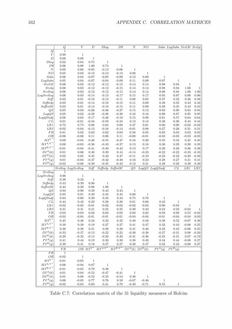
162 APPENDIX C. CORRELATION MATRICES
Q V D Dlog D$ N NO Sabs LogSabs SrelM SrelpQ 1V 0.99 1D 0.06 0.08 1
Dlog 0.02 0.04 0.75 1D$ 0.06 0.08 1.00 0.74 1N 0.69 0.66 -0.05 -0.12 -0.06 1
NO 0.05 0.03 -0.12 -0.13 -0.13 0.08 1Sabs 0.06 0.04 -0.07 -0.05 -0.09 0.12 0.09 1
LogSabs 0.05 0.04 -0.07 -0.04 -0.09 0.11 0.09 0.97 1SrelM 0.06 0.03 -0.12 -0.12 -0.15 0.14 0.14 0.98 0.94 1Srelp 0.06 0.03 -0.12 -0.12 -0.15 0.14 0.14 0.98 0.94 1.00 1
Srellog 0.06 0.03 -0.12 -0.12 -0.15 0.14 0.14 0.98 0.94 1.00 1.00LogSrellog 0.06 0.03 -0.14 -0.13 -0.17 0.15 0.17 0.95 0.97 0.96 0.96
Seff 0.02 0.01 -0.10 -0.13 -0.11 0.08 0.05 0.37 0.32 0.38 0.38Seffrelp 0.03 0.01 -0.14 -0.18 -0.15 0.11 0.09 0.39 0.35 0.43 0.43
SeffrelM 0.03 0.01 -0.14 -0.18 -0.15 0.11 0.09 0.39 0.35 0.43 0.43QS 0.05 0.03 -0.26 -0.36 -0.27 0.15 0.12 0.93 0.90 0.94 0.94
LogQS 0.05 0.02 -0.28 -0.38 -0.30 0.16 0.16 0.90 0.87 0.95 0.95LogQSadj 0.06 0.04 -0.17 -0.46 -0.18 0.15 0.09 0.61 0.57 0.64 0.64
CL 0.01 -0.01 -0.34 -0.59 -0.34 0.13 0.14 0.38 0.36 0.44 0.44LR1 0.72 0.73 0.08 0.04 0.08 0.47 0.01 0.00 0.00 -0.02 -0.02LR3 -0.02 -0.04 -0.13 -0.16 -0.14 -0.01 0.08 0.27 0.26 0.31 0.31FR 0.81 0.82 0.03 0.02 0.03 0.56 0.05 0.03 0.03 0.03 0.03OR -0.06 -0.06 0.11 0.06 0.11 -0.08 -0.01 -0.03 -0.03 -0.03 -0.03
MIV ∗ 0.00 -0.04 -0.46 -0.55 -0.47 0.16 0.20 0.35 0.34 0.45 0.45
MIA,V ∗ 0.00 -0.03 -0.36 -0.43 -0.37 0.13 0.16 0.30 0.29 0.39 0.39
MIB,V ∗ -0.01 -0.04 -0.41 -0.49 -0.42 0.13 0.17 0.29 0.28 0.36 0.36DIA(k) 0.01 0.06 0.40 0.39 0.44 -0.14 -0.23 -0.22 -0.22 -0.33 -0.33DIB(k) 0.02 0.05 0.45 0.42 0.47 -0.11 -0.19 -0.22 -0.22 -0.29 -0.29PIA(q) 0.01 -0.04 -0.37 -0.42 -0.40 0.16 0.23 0.28 0.27 0.41 0.41PIB(q) -0.02 -0.06 -0.39 -0.45 -0.42 0.12 0.21 0.29 0.28 0.39 0.39
Srellog LogSrellog Seff Seffrelp SeffrelM QS LogQS LogQSadj CL LR1 LR3Srellog 1
LogSrellog 0.96 1Seff 0.38 0.33 1
Seffrelp 0.43 0.39 0.98 1SeffrelM 0.43 0.39 0.98 1.00 1
QS 0.94 0.90 0.39 0.43 0.43 1LogQS 0.95 0.91 0.39 0.45 0.45 0.98 1
LogQSadj 0.64 0.60 0.30 0.34 0.34 0.75 0.76 1CL 0.44 0.42 0.22 0.28 0.28 0.61 0.66 0.42 1
LR1 -0.02 -0.02 -0.01 -0.02 -0.02 -0.02 -0.03 0.00 -0.04 1LR3 0.31 0.31 0.21 0.25 0.25 0.30 0.33 0.24 0.23 -0.04 1FR 0.03 0.03 0.02 0.02 0.02 0.02 0.02 0.03 0.00 0.55 -0.02OR -0.03 -0.04 -0.01 -0.01 -0.01 -0.04 -0.04 -0.01 -0.04 -0.04 0.03
MIV ∗ 0.45 0.46 0.24 0.32 0.32 0.49 0.56 0.38 0.52 -0.07 0.30
MIA,V ∗ 0.39 0.39 0.19 0.27 0.27 0.41 0.47 0.32 0.43 -0.06 0.25
MIB,V ∗ 0.36 0.38 0.21 0.28 0.28 0.41 0.46 0.32 0.43 -0.06 0.25DIA(k) -0.33 -0.37 -0.13 -0.22 -0.22 -0.30 -0.38 -0.27 -0.31 0.08 -0.20DIB(k) -0.29 -0.32 -0.14 -0.20 -0.20 -0.31 -0.36 -0.25 -0.31 0.07 -0.19PIA(q) 0.41 0.44 0.19 0.30 0.30 0.38 0.49 0.34 0.44 -0.08 0.27PIB(q) 0.39 0.41 0.18 0.27 0.27 0.40 0.47 0.32 0.43 -0.08 0.27
FR OR MIV ∗ MIA,V ∗ MIB,V ∗ DIA(k) DIB(k) PIA(q) PIB(q)FR 1OR -0.02 1
MIV ∗ -0.01 -0.05 1
MIA,V ∗ 0.00 -0.04 0.87 1
MIB,V ∗ -0.01 -0.05 0.79 0.38 1DIA(k) 0.01 0.04 -0.53 -0.47 -0.41 1DIB(k) 0.01 0.08 -0.52 -0.35 -0.54 0.36 1PIA(q) 0.00 -0.05 0.77 0.76 0.50 -0.67 -0.46 1PIB(q) -0.02 -0.04 0.69 0.41 0.79 -0.49 -0.71 0.55 1
Table C.7: Correlation matrix of the 31 liquidity measures of Holcim
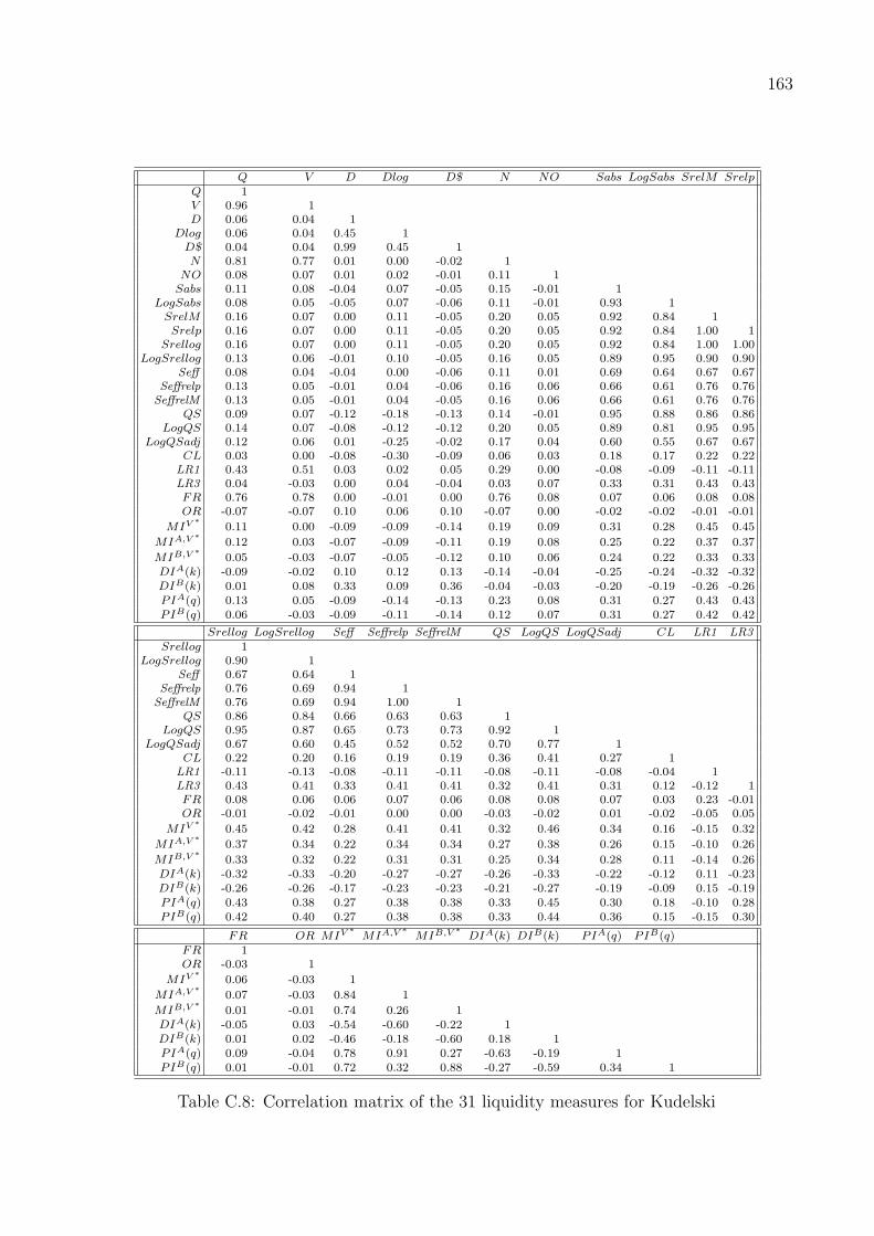
163
Q V D Dlog D$ N NO Sabs LogSabs SrelM SrelpQ 1V 0.96 1D 0.06 0.04 1
Dlog 0.06 0.04 0.45 1D$ 0.04 0.04 0.99 0.45 1N 0.81 0.77 0.01 0.00 -0.02 1
NO 0.08 0.07 0.01 0.02 -0.01 0.11 1Sabs 0.11 0.08 -0.04 0.07 -0.05 0.15 -0.01 1
LogSabs 0.08 0.05 -0.05 0.07 -0.06 0.11 -0.01 0.93 1SrelM 0.16 0.07 0.00 0.11 -0.05 0.20 0.05 0.92 0.84 1Srelp 0.16 0.07 0.00 0.11 -0.05 0.20 0.05 0.92 0.84 1.00 1
Srellog 0.16 0.07 0.00 0.11 -0.05 0.20 0.05 0.92 0.84 1.00 1.00LogSrellog 0.13 0.06 -0.01 0.10 -0.05 0.16 0.05 0.89 0.95 0.90 0.90
Seff 0.08 0.04 -0.04 0.00 -0.06 0.11 0.01 0.69 0.64 0.67 0.67Seffrelp 0.13 0.05 -0.01 0.04 -0.06 0.16 0.06 0.66 0.61 0.76 0.76
SeffrelM 0.13 0.05 -0.01 0.04 -0.05 0.16 0.06 0.66 0.61 0.76 0.76QS 0.09 0.07 -0.12 -0.18 -0.13 0.14 -0.01 0.95 0.88 0.86 0.86
LogQS 0.14 0.07 -0.08 -0.12 -0.12 0.20 0.05 0.89 0.81 0.95 0.95LogQSadj 0.12 0.06 0.01 -0.25 -0.02 0.17 0.04 0.60 0.55 0.67 0.67
CL 0.03 0.00 -0.08 -0.30 -0.09 0.06 0.03 0.18 0.17 0.22 0.22LR1 0.43 0.51 0.03 0.02 0.05 0.29 0.00 -0.08 -0.09 -0.11 -0.11LR3 0.04 -0.03 0.00 0.04 -0.04 0.03 0.07 0.33 0.31 0.43 0.43FR 0.76 0.78 0.00 -0.01 0.00 0.76 0.08 0.07 0.06 0.08 0.08OR -0.07 -0.07 0.10 0.06 0.10 -0.07 0.00 -0.02 -0.02 -0.01 -0.01
MIV ∗ 0.11 0.00 -0.09 -0.09 -0.14 0.19 0.09 0.31 0.28 0.45 0.45
MIA,V ∗ 0.12 0.03 -0.07 -0.09 -0.11 0.19 0.08 0.25 0.22 0.37 0.37
MIB,V ∗ 0.05 -0.03 -0.07 -0.05 -0.12 0.10 0.06 0.24 0.22 0.33 0.33DIA(k) -0.09 -0.02 0.10 0.12 0.13 -0.14 -0.04 -0.25 -0.24 -0.32 -0.32DIB(k) 0.01 0.08 0.33 0.09 0.36 -0.04 -0.03 -0.20 -0.19 -0.26 -0.26PIA(q) 0.13 0.05 -0.09 -0.14 -0.13 0.23 0.08 0.31 0.27 0.43 0.43PIB(q) 0.06 -0.03 -0.09 -0.11 -0.14 0.12 0.07 0.31 0.27 0.42 0.42
Srellog LogSrellog Seff Seffrelp SeffrelM QS LogQS LogQSadj CL LR1 LR3Srellog 1
LogSrellog 0.90 1Seff 0.67 0.64 1
Seffrelp 0.76 0.69 0.94 1SeffrelM 0.76 0.69 0.94 1.00 1
QS 0.86 0.84 0.66 0.63 0.63 1LogQS 0.95 0.87 0.65 0.73 0.73 0.92 1
LogQSadj 0.67 0.60 0.45 0.52 0.52 0.70 0.77 1CL 0.22 0.20 0.16 0.19 0.19 0.36 0.41 0.27 1
LR1 -0.11 -0.13 -0.08 -0.11 -0.11 -0.08 -0.11 -0.08 -0.04 1LR3 0.43 0.41 0.33 0.41 0.41 0.32 0.41 0.31 0.12 -0.12 1FR 0.08 0.06 0.06 0.07 0.06 0.08 0.08 0.07 0.03 0.23 -0.01OR -0.01 -0.02 -0.01 0.00 0.00 -0.03 -0.02 0.01 -0.02 -0.05 0.05
MIV ∗ 0.45 0.42 0.28 0.41 0.41 0.32 0.46 0.34 0.16 -0.15 0.32
MIA,V ∗ 0.37 0.34 0.22 0.34 0.34 0.27 0.38 0.26 0.15 -0.10 0.26
MIB,V ∗ 0.33 0.32 0.22 0.31 0.31 0.25 0.34 0.28 0.11 -0.14 0.26DIA(k) -0.32 -0.33 -0.20 -0.27 -0.27 -0.26 -0.33 -0.22 -0.12 0.11 -0.23DIB(k) -0.26 -0.26 -0.17 -0.23 -0.23 -0.21 -0.27 -0.19 -0.09 0.15 -0.19PIA(q) 0.43 0.38 0.27 0.38 0.38 0.33 0.45 0.30 0.18 -0.10 0.28PIB(q) 0.42 0.40 0.27 0.38 0.38 0.33 0.44 0.36 0.15 -0.15 0.30
FR OR MIV ∗ MIA,V ∗ MIB,V ∗ DIA(k) DIB(k) PIA(q) PIB(q)FR 1OR -0.03 1
MIV ∗ 0.06 -0.03 1
MIA,V ∗ 0.07 -0.03 0.84 1
MIB,V ∗ 0.01 -0.01 0.74 0.26 1DIA(k) -0.05 0.03 -0.54 -0.60 -0.22 1DIB(k) 0.01 0.02 -0.46 -0.18 -0.60 0.18 1PIA(q) 0.09 -0.04 0.78 0.91 0.27 -0.63 -0.19 1PIB(q) 0.01 -0.01 0.72 0.32 0.88 -0.27 -0.59 0.34 1
Table C.8: Correlation matrix of the 31 liquidity measures for Kudelski

164 APPENDIX C. CORRELATION MATRICES
Q V D Dlog D$ N NO Sabs LogSabs SrelM SrelpQ 1V 1.00 1D 0.03 0.04 1
Dlog 0.00 0.02 0.75 1D$ 0.02 0.04 1.00 0.76 1N 0.69 0.67 -0.07 -0.12 -0.08 1
NO 0.07 0.06 -0.11 -0.13 -0.12 0.10 1Sabs 0.05 0.06 0.09 0.16 0.09 0.08 -0.02 1
LogSabs 0.03 0.04 0.15 0.25 0.15 0.02 -0.08 0.91 1SrelM 0.07 0.06 0.02 0.05 0.01 0.12 0.04 0.97 0.86 1Srelp 0.07 0.06 0.02 0.05 0.01 0.12 0.04 0.97 0.86 1.00 1
Srellog 0.07 0.06 0.02 0.05 0.01 0.12 0.04 0.97 0.86 1.00 1.00LogSrellog 0.05 0.05 0.08 0.15 0.08 0.07 -0.01 0.92 0.98 0.91 0.91
Seff -0.01 -0.02 -0.05 -0.06 -0.06 0.03 -0.01 0.46 0.42 0.50 0.50Seffrelp 0.00 -0.01 -0.10 -0.13 -0.11 0.07 0.04 0.49 0.42 0.56 0.56
SeffrelM 0.00 -0.01 -0.10 -0.13 -0.11 0.07 0.04 0.49 0.42 0.56 0.56QS 0.05 0.04 -0.13 -0.17 -0.13 0.12 0.02 0.93 0.83 0.95 0.95
LogQS 0.06 0.04 -0.18 -0.24 -0.19 0.15 0.07 0.88 0.75 0.94 0.94LogQSadj 0.04 0.03 -0.13 -0.46 -0.14 0.12 0.05 0.45 0.39 0.51 0.51
CL 0.02 0.00 -0.26 -0.47 -0.26 0.10 0.08 0.20 0.14 0.28 0.28LR1 0.70 0.70 -0.01 -0.03 -0.02 0.48 0.07 0.01 -0.03 0.02 0.02LR3 -0.01 -0.02 -0.07 -0.10 -0.08 0.03 0.05 0.10 0.06 0.13 0.13FR 0.86 0.86 0.01 0.01 0.00 0.62 0.05 0.05 0.03 0.05 0.05OR -0.07 -0.07 0.11 0.07 0.11 -0.09 -0.03 -0.01 0.00 -0.02 -0.02
MIV ∗ 0.04 0.02 -0.17 -0.23 -0.18 0.12 0.07 0.07 -0.02 0.14 0.14
MIA,V ∗ 0.05 0.02 -0.26 -0.34 -0.28 0.15 0.13 0.10 -0.03 0.20 0.20
MIB,V ∗ 0.03 0.01 -0.09 -0.12 -0.10 0.07 0.03 0.04 0.00 0.08 0.08DIA(k) 0.05 0.07 0.44 0.42 0.44 -0.03 -0.10 -0.03 0.07 -0.12 -0.12DIB(k) 0.08 0.11 0.48 0.45 0.49 -0.04 -0.06 -0.04 0.06 -0.12 -0.12PIA(q) 0.05 0.02 -0.30 -0.40 -0.31 0.16 0.16 0.11 -0.05 0.23 0.23PIB(q) 0.02 0.00 -0.12 -0.16 -0.12 0.07 0.03 0.06 0.01 0.12 0.12
Srellog LogSrellog Seff Seffrelp SeffrelM QS LogQS LogQSadj CL LR1 LR3Srellog 1
LogSrellog 0.91 1Seff 0.50 0.45 1
Seffrelp 0.56 0.48 0.98 1SeffrelM 0.56 0.48 0.98 1.00 1
QS 0.95 0.88 0.51 0.56 0.56 1LogQS 0.94 0.84 0.52 0.60 0.60 0.98 1
LogQSadj 0.51 0.45 0.33 0.39 0.39 0.65 0.68 1CL 0.28 0.22 0.21 0.28 0.28 0.45 0.51 0.38 1
LR1 0.02 -0.01 -0.02 0.00 0.00 0.01 0.03 0.02 0.03 1LR3 0.13 0.10 0.15 0.17 0.17 0.13 0.16 0.12 0.10 0.01 1FR 0.05 0.04 -0.01 0.00 0.00 0.04 0.04 0.02 0.01 0.60 -0.02OR -0.02 -0.01 0.01 0.00 0.00 -0.03 -0.04 0.00 -0.03 -0.05 0.11
MIV ∗ 0.14 0.06 0.08 0.13 0.13 0.15 0.20 0.18 0.16 0.02 0.09
MIA,V ∗ 0.20 0.07 0.12 0.20 0.20 0.21 0.30 0.24 0.25 0.05 0.11
MIB,V ∗ 0.08 0.04 0.04 0.07 0.07 0.08 0.11 0.11 0.08 0.00 0.06DIA(k) -0.12 -0.02 -0.08 -0.15 -0.15 -0.16 -0.22 -0.16 -0.23 0.01 -0.09DIB(k) -0.12 -0.02 -0.09 -0.15 -0.15 -0.17 -0.23 -0.17 -0.22 0.02 -0.09PIA(q) 0.23 0.07 0.15 0.24 0.24 0.25 0.35 0.28 0.31 0.06 0.15PIB(q) 0.12 0.06 0.07 0.12 0.12 0.13 0.18 0.17 0.12 0.01 0.08
FR OR MIV ∗ MIA,V ∗ MIB,V ∗ DIA(k) DIB(k) PIA(q) PIB(q)FR 1OR -0.04 1
MIV ∗ 0.03 -0.02 1
MIA,V ∗ 0.03 -0.03 0.41 1
MIB,V ∗ 0.02 -0.01 0.94 0.08 1DIA(k) 0.03 0.03 -0.20 -0.33 -0.10 1DIB(k) 0.06 0.05 -0.21 -0.25 -0.13 0.34 1PIA(q) 0.02 -0.04 0.40 0.90 0.10 -0.40 -0.31 1PIB(q) 0.01 -0.02 0.67 0.10 0.69 -0.13 -0.19 0.14 1
Table C.9: Correlation matrix of the 31 liquidity measures for Lonza

165
Q V D Dlog D$ N NO Sabs LogSabs SrelM SrelpQ 1V 0.99 1D -0.07 -0.04 1
Dlog -0.08 -0.06 0.73 1D$ -0.10 -0.06 0.99 0.71 1N 0.81 0.78 -0.17 -0.16 -0.21 1
NO 0.73 0.69 -0.21 -0.19 -0.25 0.89 1Sabs 0.12 0.10 0.08 0.13 0.06 0.13 0.14 1
LogSabs 0.11 0.10 0.10 0.15 0.07 0.12 0.13 0.98 1SrelM 0.19 0.14 -0.02 0.05 -0.08 0.23 0.26 0.94 0.91 1Srelp 0.19 0.14 -0.02 0.05 -0.08 0.23 0.26 0.94 0.91 1.00 1
Srellog 0.19 0.14 -0.02 0.05 -0.08 0.23 0.26 0.94 0.91 1.00 1.00LogSrellog 0.21 0.16 -0.03 0.04 -0.10 0.26 0.29 0.91 0.91 0.97 0.97
Seff 0.06 0.04 -0.07 -0.05 -0.09 0.10 0.13 0.39 0.35 0.44 0.44Seffrelp 0.12 0.08 -0.13 -0.09 -0.18 0.19 0.23 0.44 0.40 0.58 0.58
SeffrelM 0.12 0.08 -0.13 -0.09 -0.18 0.19 0.23 0.44 0.40 0.58 0.58QS 0.15 0.13 -0.16 -0.23 -0.18 0.18 0.21 0.93 0.90 0.90 0.90
LogQS 0.21 0.15 -0.21 -0.25 -0.26 0.28 0.31 0.86 0.83 0.95 0.95LogQSadj 0.12 0.10 -0.23 -0.68 -0.25 0.16 0.18 0.30 0.28 0.36 0.36
CL 0.18 0.14 -0.41 -0.49 -0.41 0.28 0.30 0.24 0.22 0.35 0.35LR1 0.59 0.63 0.00 -0.03 -0.01 0.48 0.39 0.03 0.03 0.02 0.02LR3 -0.04 -0.08 -0.13 -0.09 -0.16 0.02 0.10 0.18 0.16 0.29 0.29FR 0.89 0.88 -0.07 -0.07 -0.08 0.70 0.63 0.09 0.09 0.13 0.13OR -0.03 -0.03 0.02 0.01 0.02 -0.04 -0.04 -0.01 -0.01 -0.02 -0.02
MIV ∗ 0.18 0.13 -0.44 -0.55 -0.46 0.32 0.35 0.32 0.30 0.45 0.45
MIA,V ∗ 0.14 0.11 -0.33 -0.48 -0.35 0.21 0.24 0.21 0.20 0.29 0.29
MIB,V ∗ 0.13 0.09 -0.33 -0.35 -0.34 0.26 0.29 0.27 0.25 0.37 0.37DIA(k) -0.19 -0.13 0.44 0.37 0.50 -0.29 -0.36 -0.14 -0.13 -0.32 -0.32DIB(k) -0.12 -0.06 0.43 0.36 0.47 -0.22 -0.27 -0.12 -0.11 -0.26 -0.26PIA(q) 0.20 0.14 -0.43 -0.49 -0.46 0.31 0.35 0.23 0.22 0.38 0.38PIB(q) 0.15 0.09 -0.40 -0.38 -0.43 0.30 0.34 0.28 0.26 0.43 0.43
Srellog LogSrellog Seff Seffrelp SeffrelM QS LogQS LogQSadj CL LR1 LR3Srellog 1
LogSrellog 0.97 1Seff 0.44 0.37 1
Seffrelp 0.58 0.51 0.96 1SeffrelM 0.58 0.51 0.96 1.00 1
QS 0.90 0.87 0.41 0.48 0.48 1LogQS 0.95 0.92 0.45 0.60 0.60 0.95 1
LogQSadj 0.36 0.34 0.24 0.30 0.30 0.58 0.58 1CL 0.35 0.34 0.20 0.31 0.31 0.44 0.52 0.34 1
LR1 0.02 0.03 0.00 -0.01 -0.01 0.03 0.02 0.03 0.01 1LR3 0.29 0.29 0.21 0.30 0.31 0.21 0.31 0.15 0.20 -0.12 1FR 0.13 0.14 0.06 0.10 0.10 0.12 0.15 0.09 0.18 0.45 -0.02OR -0.02 -0.02 0.00 -0.01 -0.01 -0.02 -0.02 -0.01 -0.02 -0.02 0.03
MIV ∗ 0.45 0.45 0.22 0.35 0.35 0.51 0.60 0.48 0.58 0.01 0.27
MIA,V ∗ 0.29 0.31 0.13 0.21 0.22 0.38 0.42 0.41 0.43 0.02 0.15
MIB,V ∗ 0.37 0.36 0.20 0.30 0.30 0.38 0.46 0.31 0.44 0.00 0.25DIA(k) -0.32 -0.37 -0.16 -0.31 -0.31 -0.26 -0.41 -0.28 -0.35 -0.01 -0.27DIB(k) -0.26 -0.30 -0.14 -0.26 -0.26 -0.24 -0.35 -0.25 -0.31 0.03 -0.23PIA(q) 0.38 0.41 0.18 0.32 0.32 0.40 0.52 0.41 0.50 0.01 0.27PIB(q) 0.43 0.43 0.23 0.37 0.37 0.41 0.53 0.33 0.49 -0.01 0.32
FR OR MIV ∗ MIA,V ∗ MIB,V ∗ DIA(k) DIB(k) PIA(q) PIB(q)FR 1OR -0.01 1
MIV ∗ 0.14 -0.02 1
MIA,V ∗ 0.10 -0.02 0.70 1
MIB,V ∗ 0.11 -0.01 0.78 0.10 1DIA(k) -0.14 0.04 -0.46 -0.38 -0.31 1DIB(k) -0.09 0.00 -0.41 -0.25 -0.35 0.41 1PIA(q) 0.14 -0.02 0.71 0.86 0.22 -0.54 -0.39 1PIB(q) 0.12 -0.01 0.74 0.17 0.89 -0.42 -0.47 0.33 1
Table C.10: Correlation matrix of the 31 liquidity measures of Swiss Re
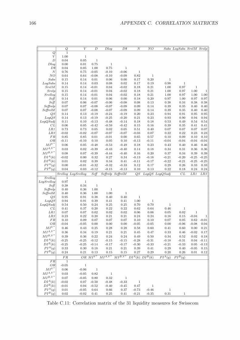
166 APPENDIX C. CORRELATION MATRICES
Q V D Dlog D$ N NO Sabs LogSabs SrelM SrelpQ 1V 1.00 1D 0.04 0.05 1
Dlog 0.00 0.01 0.75 1D$ 0.04 0.05 1.00 0.75 1N 0.76 0.75 -0.05 -0.10 -0.06 1
NO 0.64 0.64 -0.08 -0.10 -0.09 0.82 1Sabs 0.15 0.14 0.01 0.06 0.00 0.17 0.20 1
LogSabs 0.14 0.14 0.03 0.08 0.02 0.17 0.19 0.98 1SrelM 0.15 0.14 -0.01 0.04 -0.02 0.18 0.21 1.00 0.97 1Srelp 0.15 0.14 -0.01 0.04 -0.02 0.18 0.21 1.00 0.97 1.00 1
Srellog 0.15 0.14 -0.01 0.04 -0.02 0.18 0.21 1.00 0.97 1.00 1.00Seff 0.14 0.14 0.01 0.06 0.00 0.18 0.20 0.97 1.00 0.97 0.97Seff 0.07 0.06 -0.07 -0.06 -0.08 0.08 0.13 0.38 0.34 0.38 0.38
Seffrelp 0.07 0.07 -0.08 -0.07 -0.09 0.09 0.14 0.39 0.35 0.40 0.40SeffrelM 0.07 0.07 -0.08 -0.07 -0.09 0.09 0.14 0.39 0.35 0.40 0.40
QS 0.14 0.13 -0.19 -0.24 -0.19 0.20 0.23 0.94 0.91 0.95 0.95LogQS 0.14 0.13 -0.19 -0.25 -0.20 0.21 0.23 0.93 0.90 0.94 0.94
LogQSadj 0.11 0.10 -0.13 -0.48 -0.14 0.18 0.18 0.53 0.49 0.54 0.54CL 0.06 0.05 -0.42 -0.59 -0.42 0.15 0.16 0.39 0.35 0.41 0.41
LR1 0.73 0.73 0.05 0.02 0.05 0.51 0.40 0.07 0.07 0.07 0.07LR3 -0.02 -0.02 -0.07 -0.07 -0.07 -0.03 0.07 0.22 0.22 0.23 0.23FR 0.85 0.85 0.01 -0.01 0.00 0.65 0.57 0.10 0.09 0.10 0.10OR -0.11 -0.10 0.10 0.05 0.10 -0.13 -0.11 -0.04 -0.04 -0.04 -0.04
MIV ∗ 0.06 0.05 -0.48 -0.53 -0.49 0.18 0.23 0.43 0.40 0.46 0.46
MIA,V ∗ 0.03 0.02 -0.39 -0.43 -0.40 0.14 0.18 0.34 0.31 0.36 0.36
MIB,V ∗ 0.08 0.07 -0.39 -0.44 -0.40 0.16 0.20 0.37 0.34 0.39 0.39DIA(k) -0.02 0.00 0.32 0.27 0.34 -0.13 -0.18 -0.21 -0.20 -0.25 -0.25DIB(k) 0.01 0.02 0.39 0.34 0.41 -0.11 -0.17 -0.22 -0.21 -0.25 -0.25PIA(q) 0.00 -0.01 -0.32 -0.32 -0.33 0.12 0.17 0.29 0.26 0.33 0.33PIB(q) 0.04 0.03 -0.12 -0.15 -0.13 0.10 0.13 0.22 0.18 0.24 0.24
Srellog LogSrellog Seff Seffrelp SeffrelM QS LogQS LogQSadj CL LR1 LR3Srellog 1
LogSrellog 0.97 1Seff 0.38 0.34 1
Seffrelp 0.40 0.36 1.00 1SeffrelM 0.40 0.36 1.00 1.00 1
QS 0.95 0.91 0.38 0.40 0.40 1LogQS 0.94 0.91 0.39 0.41 0.41 1.00 1
LogQSadj 0.54 0.50 0.24 0.25 0.25 0.70 0.70 1CL 0.41 0.37 0.20 0.22 0.22 0.62 0.64 0.46 1
LR1 0.07 0.07 0.02 0.02 0.02 0.06 0.06 0.05 0.02 1LR3 0.23 0.22 0.20 0.21 0.21 0.24 0.24 0.16 0.15 -0.04 1FR 0.10 0.09 0.07 0.07 0.07 0.10 0.10 0.07 0.05 0.62 -0.01OR -0.04 -0.05 0.00 0.00 0.00 -0.05 -0.05 0.00 -0.06 -0.08 0.04
MIV ∗ 0.46 0.43 0.25 0.28 0.28 0.58 0.60 0.41 0.60 0.00 0.21
MIA,V ∗ 0.36 0.34 0.19 0.21 0.21 0.45 0.47 0.33 0.46 -0.02 0.17
MIB,V ∗ 0.39 0.36 0.22 0.24 0.24 0.49 0.50 0.34 0.52 0.02 0.18DIA(k) -0.25 -0.25 -0.12 -0.15 -0.15 -0.28 -0.31 -0.18 -0.31 0.04 -0.11DIB(k) -0.25 -0.25 -0.14 -0.17 -0.17 -0.30 -0.33 -0.21 -0.33 0.05 -0.13PIA(q) 0.33 0.30 0.18 0.21 0.21 0.39 0.41 0.29 0.40 -0.05 0.15PIB(q) 0.24 0.21 0.13 0.15 0.15 0.27 0.29 0.20 0.26 0.01 0.12
FR OR MIV ∗ MIA,V ∗ MIB,V ∗ DIA(k) DIB(k) PIA(q) PIB(q)FR 1OR -0.05 1
MIV ∗ 0.06 -0.06 1
MIA,V ∗ 0.03 -0.05 0.82 1
MIB,V ∗ 0.07 -0.05 0.80 0.32 1DIA(k) -0.02 0.07 -0.50 -0.48 -0.33 1DIB(k) -0.01 0.04 -0.52 -0.40 -0.45 0.47 1PIA(q) 0.01 -0.05 0.64 0.66 0.37 -0.73 -0.46 1PIB(q) 0.02 -0.02 0.41 0.25 0.41 -0.21 -0.35 0.31 1
Table C.11: Correlation matrix of the 31 liquidity measures for Swisscom
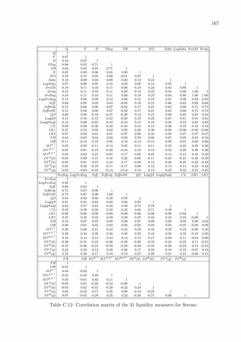
167
Q V D Dlog D$ N NO Sabs LogSabs SrelM SrelpQ 1V 0.97 1D 0.10 0.07 1
Dlog 0.06 0.03 0.71 1D$ 0.04 0.05 0.95 0.71 1N 0.85 0.83 0.06 0.01 0.00 1
NO 0.76 0.74 0.05 0.00 -0.01 0.87 1Sabs 0.10 0.08 0.04 0.09 0.02 0.12 0.16 1
LogSabs 0.07 0.06 0.05 0.10 0.03 0.08 0.12 0.95 1SrelM 0.18 0.11 0.10 0.11 0.00 0.19 0.23 0.94 0.88 1Srelp 0.18 0.11 0.10 0.11 0.00 0.19 0.23 0.94 0.88 1.00 1
Srellog 0.18 0.11 0.10 0.11 0.00 0.19 0.23 0.94 0.88 1.00 1.00LogSrellog 0.13 0.08 0.09 0.12 0.00 0.15 0.19 0.91 0.96 0.92 0.93
Seff 0.08 0.05 0.03 0.04 -0.02 0.10 0.15 0.66 0.62 0.68 0.68Seffrelp 0.15 0.08 0.08 0.07 -0.02 0.17 0.21 0.65 0.60 0.75 0.75
SeffrelM 0.15 0.08 0.08 0.07 -0.02 0.17 0.21 0.65 0.60 0.75 0.75QS 0.09 0.08 -0.18 -0.27 -0.20 0.12 0.15 0.90 0.85 0.84 0.84
LogQS 0.15 0.10 -0.12 -0.22 -0.20 0.19 0.22 0.87 0.81 0.91 0.91LogQSadj 0.13 0.09 -0.04 -0.34 -0.10 0.15 0.16 0.58 0.53 0.63 0.63
CL 0.09 0.06 -0.30 -0.49 -0.34 0.13 0.14 0.38 0.35 0.42 0.42LR1 0.47 0.53 0.03 0.02 0.05 0.36 0.30 -0.06 -0.06 -0.08 -0.08LR3 0.07 0.02 0.01 0.01 -0.07 0.06 0.16 0.29 0.27 0.37 0.37FR 0.84 0.85 0.04 0.02 0.02 0.79 0.66 0.07 0.05 0.10 0.10OR -0.11 -0.12 0.10 0.06 0.10 -0.13 -0.12 0.00 0.01 0.00 0.00
MIV ∗ 0.05 0.02 0.11 -0.14 0.05 0.11 0.11 0.25 0.22 0.28 0.28
MIA,V ∗ 0.05 0.01 -0.19 -0.20 -0.24 0.10 0.13 0.32 0.28 0.36 0.36
MIB,V ∗ 0.03 0.02 0.21 -0.07 0.17 0.08 0.07 0.14 0.12 0.16 0.16DIA(k) -0.05 0.00 0.15 0.16 0.22 -0.08 -0.11 -0.25 -0.24 -0.30 -0.30DIB(k) -0.05 0.01 0.07 0.10 0.17 -0.08 -0.12 -0.26 -0.25 -0.33 -0.33PIA(q) 0.07 0.02 -0.10 -0.11 -0.17 0.09 0.12 0.14 0.14 0.22 0.22PIB(q) 0.05 0.03 -0.10 -0.14 -0.13 0.12 0.13 0.23 0.22 0.25 0.25
Srellog LogSrellog Seff Seffrelp SeffrelM QS LogQS LogQSadj CL LR1 LR3Srellog 1
LogSrellog 0.92 1Seff 0.68 0.63 1
Seffrelp 0.75 0.67 0.96 1SeffrelM 0.75 0.67 0.96 1.00 1
QS 0.84 0.82 0.60 0.58 0.58 1LogQS 0.91 0.84 0.62 0.68 0.68 0.95 1
LogQSadj 0.63 0.57 0.44 0.49 0.49 0.74 0.79 1CL 0.42 0.39 0.28 0.32 0.32 0.68 0.71 0.49 1
LR1 -0.08 -0.08 -0.08 -0.09 -0.09 -0.06 -0.08 -0.06 -0.04 1LR3 0.37 0.35 0.33 0.39 0.39 0.27 0.34 0.24 0.19 -0.08 1FR 0.10 0.07 0.07 0.09 0.09 0.07 0.09 0.08 0.05 0.30 0.02OR 0.00 0.01 0.03 0.02 0.02 -0.02 -0.02 0.03 -0.05 -0.09 0.09
MIV ∗ 0.28 0.26 0.21 0.24 0.24 0.29 0.32 0.29 0.23 -0.08 0.16
MIA,V ∗ 0.36 0.34 0.26 0.30 0.30 0.39 0.42 0.30 0.35 -0.10 0.20
MIB,V ∗ 0.16 0.14 0.12 0.14 0.14 0.15 0.17 0.20 0.11 -0.04 0.09DIA(k) -0.30 -0.31 -0.23 -0.26 -0.26 -0.29 -0.33 -0.24 -0.25 0.11 -0.21DIB(k) -0.33 -0.36 -0.24 -0.29 -0.29 -0.28 -0.35 -0.26 -0.23 0.12 -0.24PIA(q) 0.22 0.23 0.14 0.20 0.20 0.17 0.24 0.18 0.19 -0.07 0.18PIB(q) 0.25 0.26 0.17 0.18 0.18 0.27 0.29 0.21 0.21 -0.06 0.15
FR OR MIV ∗ MIA,V ∗ MIB,V ∗ DIA(k) DIB(k) PIA(q) PIB(q)FR 1OR -0.05 1
MIV ∗ 0.04 -0.02 1
MIA,V ∗ 0.04 -0.03 0.48 1
MIB,V ∗ 0.03 -0.01 0.92 0.11 1DIA(k) -0.04 0.01 -0.28 -0.52 -0.08 1DIB(k) -0.03 0.02 -0.31 -0.29 -0.22 0.34 1PIA(q) 0.03 -0.02 0.17 0.26 0.08 -0.44 -0.25 1PIB(q) 0.07 -0.05 0.29 0.25 0.22 -0.26 -0.57 0.09 1
Table C.12: Correlation matrix of the 31 liquidity measures for Serono

168 APPENDIX C. CORRELATION MATRICES
Q V D Dlog D$ N NO Sabs LogSabs SrelM SrelpQ 1V 0.99 1D 0.03 0.03 1
Dlog 0.05 0.05 0.22 1D$ 0.03 0.03 1.00 0.21 1N 0.72 0.71 0.02 -0.02 0.02 1
NO 0.63 0.62 0.00 -0.04 -0.01 0.83 1Sabs 0.11 0.11 -0.01 0.13 -0.01 0.07 0.18 1
LogSabs 0.09 0.09 -0.02 0.15 -0.02 0.03 0.13 0.90 1SrelM 0.14 0.12 -0.01 0.12 -0.02 0.11 0.23 0.99 0.88 1Srelp 0.14 0.12 -0.01 0.12 -0.02 0.11 0.23 0.99 0.88 1.00 1
Srellog 0.14 0.12 -0.01 0.12 -0.02 0.11 0.23 0.99 0.88 1.00 1.00LogSrellog 0.11 0.10 -0.03 0.15 -0.03 0.07 0.17 0.90 0.99 0.90 0.90
Seff 0.03 0.03 -0.01 0.03 -0.01 0.01 0.15 0.65 0.55 0.64 0.64Seffrelp 0.05 0.04 -0.02 0.03 -0.02 0.04 0.18 0.65 0.55 0.66 0.66
SeffrelM 0.05 0.04 -0.02 0.03 -0.02 0.04 0.18 0.65 0.55 0.66 0.66QS 0.09 0.09 -0.05 -0.15 -0.05 0.08 0.19 0.93 0.83 0.92 0.92
LogQS 0.12 0.11 -0.05 -0.16 -0.05 0.12 0.23 0.92 0.81 0.93 0.93LogQSadj 0.11 0.10 -0.01 -0.28 -0.01 0.12 0.20 0.64 0.57 0.66 0.66
CL 0.06 0.05 -0.06 -0.42 -0.05 0.10 0.16 0.38 0.30 0.41 0.41LR1 0.60 0.61 0.03 0.04 0.03 0.50 0.38 0.01 0.00 0.02 0.02LR3 0.10 0.09 -0.01 0.00 -0.01 0.11 0.21 0.24 0.24 0.25 0.25FR 0.86 0.87 0.02 0.04 0.01 0.64 0.55 0.08 0.07 0.10 0.10OR -0.03 -0.03 0.09 0.10 0.09 -0.04 -0.03 -0.01 -0.01 -0.01 -0.01
MIV ∗ 0.08 0.05 -0.05 -0.19 -0.05 0.14 0.21 0.28 0.22 0.31 0.31
MIA,V ∗ -0.01 -0.02 -0.06 -0.21 -0.06 0.06 0.14 0.24 0.21 0.26 0.26
MIB,V ∗ 0.09 0.07 -0.03 -0.12 -0.03 0.13 0.18 0.22 0.17 0.24 0.24DIA(k) 0.07 0.08 0.87 0.17 0.87 0.03 -0.01 -0.09 -0.09 -0.10 -0.10DIB(k) 0.14 0.15 0.11 0.23 0.11 0.07 0.04 -0.16 -0.14 -0.16 -0.16PIA(q) 0.01 0.01 -0.05 -0.13 -0.05 0.01 0.04 0.18 0.18 0.17 0.18PIB(q) -0.04 -0.05 -0.03 -0.11 -0.03 0.01 0.06 0.14 0.10 0.17 0.17
Srellog LogSrellog Seff Seffrelp SeffrelM QS LogQS LogQSadj CL LR1 LR3Srellog 1
LogSrellog 0.90 1Seff 0.64 0.55 1
Seffrelp 0.66 0.56 0.99 1SeffrelM 0.66 0.56 0.99 1.00 1
QS 0.92 0.83 0.62 0.62 0.62 1LogQS 0.93 0.83 0.61 0.62 0.63 0.99 1
LogQSadj 0.66 0.59 0.42 0.44 0.44 0.76 0.77 1CL 0.41 0.32 0.28 0.30 0.31 0.63 0.66 0.41 1
LR1 0.02 0.01 -0.05 -0.03 -0.03 0.00 0.01 0.02 0.01 1LR3 0.25 0.25 0.21 0.22 0.22 0.23 0.24 0.19 0.12 0.04 1FR 0.10 0.08 0.04 0.05 0.05 0.07 0.08 0.08 0.03 0.40 0.04OR -0.01 -0.01 0.00 0.00 0.00 -0.03 -0.03 0.00 -0.03 -0.03 0.06
MIV ∗ 0.31 0.25 0.24 0.26 0.26 0.33 0.36 0.31 0.25 -0.02 0.11
MIA,V ∗ 0.26 0.24 0.21 0.23 0.23 0.29 0.31 0.22 0.22 -0.04 0.11
MIB,V ∗ 0.24 0.18 0.18 0.20 0.20 0.25 0.27 0.26 0.19 0.00 0.08DIA(k) -0.10 -0.10 -0.07 -0.08 -0.08 -0.11 -0.12 -0.08 -0.08 0.06 -0.04DIB(k) -0.16 -0.14 -0.13 -0.13 -0.13 -0.20 -0.20 -0.13 -0.15 0.14 -0.04PIA(q) 0.17 0.19 0.15 0.14 0.14 0.22 0.20 0.18 0.10 -0.04 0.03PIB(q) 0.17 0.13 0.11 0.14 0.14 0.17 0.20 0.15 0.16 -0.06 0.06
FR OR MIV ∗ MIA,V ∗ MIB,V ∗ DIA(k) DIB(k) PIA(q) PIB(q)FR 1OR -0.02 1
MIV ∗ 0.07 -0.02 1
MIA,V ∗ -0.01 -0.04 0.50 1
MIB,V ∗ 0.09 -0.01 0.92 0.14 1DIA(k) 0.05 0.08 -0.17 -0.28 -0.07 1DIB(k) 0.09 0.02 -0.30 -0.13 -0.29 0.14 1PIA(q) 0.03 -0.03 0.25 0.33 0.14 -0.20 -0.17 1PIB(q) -0.03 0.02 0.35 0.11 0.35 -0.08 -0.53 0.03 1
Table C.13: Correlation matrix of the 31 liquidity measures for Surveillance
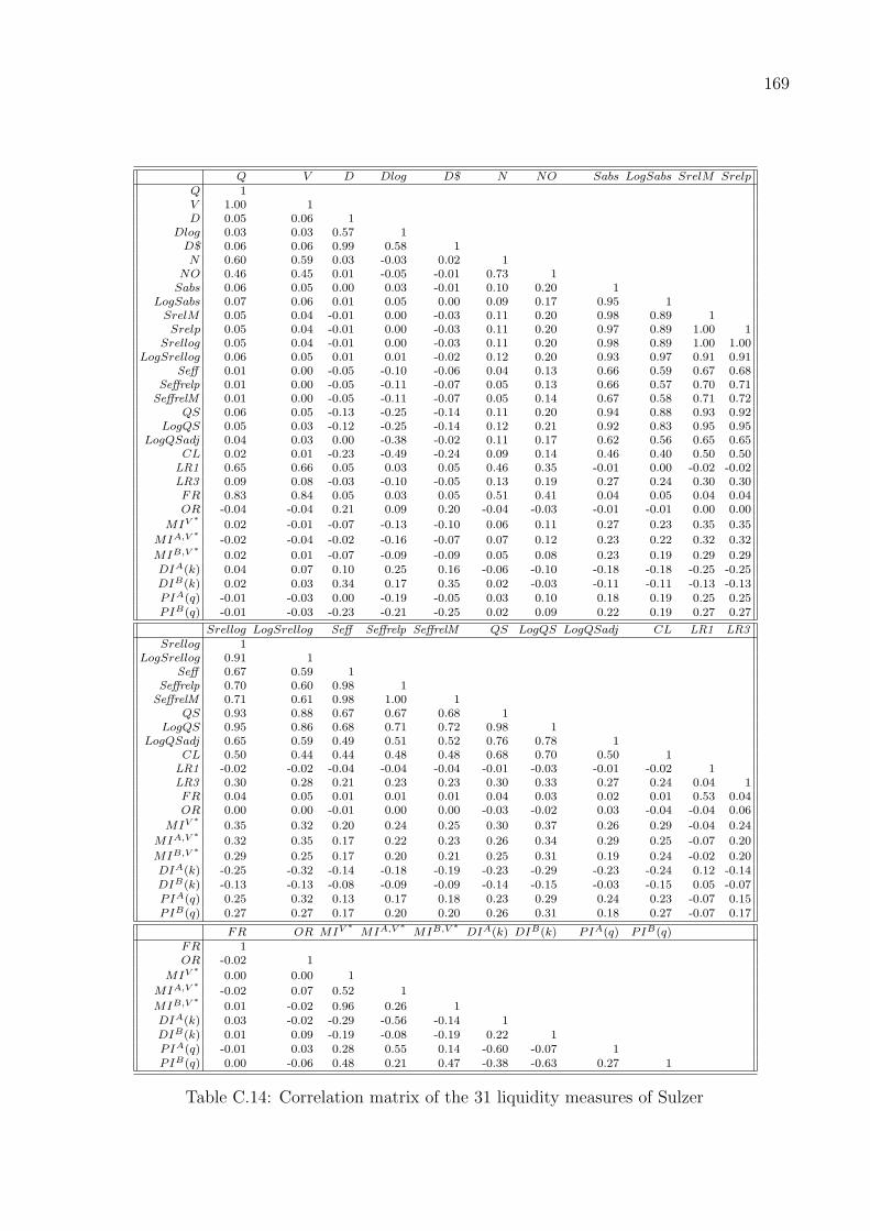
169
Q V D Dlog D$ N NO Sabs LogSabs SrelM SrelpQ 1V 1.00 1D 0.05 0.06 1
Dlog 0.03 0.03 0.57 1D$ 0.06 0.06 0.99 0.58 1N 0.60 0.59 0.03 -0.03 0.02 1
NO 0.46 0.45 0.01 -0.05 -0.01 0.73 1Sabs 0.06 0.05 0.00 0.03 -0.01 0.10 0.20 1
LogSabs 0.07 0.06 0.01 0.05 0.00 0.09 0.17 0.95 1SrelM 0.05 0.04 -0.01 0.00 -0.03 0.11 0.20 0.98 0.89 1Srelp 0.05 0.04 -0.01 0.00 -0.03 0.11 0.20 0.97 0.89 1.00 1
Srellog 0.05 0.04 -0.01 0.00 -0.03 0.11 0.20 0.98 0.89 1.00 1.00LogSrellog 0.06 0.05 0.01 0.01 -0.02 0.12 0.20 0.93 0.97 0.91 0.91
Seff 0.01 0.00 -0.05 -0.10 -0.06 0.04 0.13 0.66 0.59 0.67 0.68Seffrelp 0.01 0.00 -0.05 -0.11 -0.07 0.05 0.13 0.66 0.57 0.70 0.71
SeffrelM 0.01 0.00 -0.05 -0.11 -0.07 0.05 0.14 0.67 0.58 0.71 0.72QS 0.06 0.05 -0.13 -0.25 -0.14 0.11 0.20 0.94 0.88 0.93 0.92
LogQS 0.05 0.03 -0.12 -0.25 -0.14 0.12 0.21 0.92 0.83 0.95 0.95LogQSadj 0.04 0.03 0.00 -0.38 -0.02 0.11 0.17 0.62 0.56 0.65 0.65
CL 0.02 0.01 -0.23 -0.49 -0.24 0.09 0.14 0.46 0.40 0.50 0.50LR1 0.65 0.66 0.05 0.03 0.05 0.46 0.35 -0.01 0.00 -0.02 -0.02LR3 0.09 0.08 -0.03 -0.10 -0.05 0.13 0.19 0.27 0.24 0.30 0.30FR 0.83 0.84 0.05 0.03 0.05 0.51 0.41 0.04 0.05 0.04 0.04OR -0.04 -0.04 0.21 0.09 0.20 -0.04 -0.03 -0.01 -0.01 0.00 0.00
MIV ∗ 0.02 -0.01 -0.07 -0.13 -0.10 0.06 0.11 0.27 0.23 0.35 0.35
MIA,V ∗ -0.02 -0.04 -0.02 -0.16 -0.07 0.07 0.12 0.23 0.22 0.32 0.32
MIB,V ∗ 0.02 0.01 -0.07 -0.09 -0.09 0.05 0.08 0.23 0.19 0.29 0.29DIA(k) 0.04 0.07 0.10 0.25 0.16 -0.06 -0.10 -0.18 -0.18 -0.25 -0.25DIB(k) 0.02 0.03 0.34 0.17 0.35 0.02 -0.03 -0.11 -0.11 -0.13 -0.13PIA(q) -0.01 -0.03 0.00 -0.19 -0.05 0.03 0.10 0.18 0.19 0.25 0.25PIB(q) -0.01 -0.03 -0.23 -0.21 -0.25 0.02 0.09 0.22 0.19 0.27 0.27
Srellog LogSrellog Seff Seffrelp SeffrelM QS LogQS LogQSadj CL LR1 LR3Srellog 1
LogSrellog 0.91 1Seff 0.67 0.59 1
Seffrelp 0.70 0.60 0.98 1SeffrelM 0.71 0.61 0.98 1.00 1
QS 0.93 0.88 0.67 0.67 0.68 1LogQS 0.95 0.86 0.68 0.71 0.72 0.98 1
LogQSadj 0.65 0.59 0.49 0.51 0.52 0.76 0.78 1CL 0.50 0.44 0.44 0.48 0.48 0.68 0.70 0.50 1
LR1 -0.02 -0.02 -0.04 -0.04 -0.04 -0.01 -0.03 -0.01 -0.02 1LR3 0.30 0.28 0.21 0.23 0.23 0.30 0.33 0.27 0.24 0.04 1FR 0.04 0.05 0.01 0.01 0.01 0.04 0.03 0.02 0.01 0.53 0.04OR 0.00 0.00 -0.01 0.00 0.00 -0.03 -0.02 0.03 -0.04 -0.04 0.06
MIV ∗ 0.35 0.32 0.20 0.24 0.25 0.30 0.37 0.26 0.29 -0.04 0.24
MIA,V ∗ 0.32 0.35 0.17 0.22 0.23 0.26 0.34 0.29 0.25 -0.07 0.20
MIB,V ∗ 0.29 0.25 0.17 0.20 0.21 0.25 0.31 0.19 0.24 -0.02 0.20DIA(k) -0.25 -0.32 -0.14 -0.18 -0.19 -0.23 -0.29 -0.23 -0.24 0.12 -0.14DIB(k) -0.13 -0.13 -0.08 -0.09 -0.09 -0.14 -0.15 -0.03 -0.15 0.05 -0.07PIA(q) 0.25 0.32 0.13 0.17 0.18 0.23 0.29 0.24 0.23 -0.07 0.15PIB(q) 0.27 0.27 0.17 0.20 0.20 0.26 0.31 0.18 0.27 -0.07 0.17
FR OR MIV ∗ MIA,V ∗ MIB,V ∗ DIA(k) DIB(k) PIA(q) PIB(q)FR 1OR -0.02 1
MIV ∗ 0.00 0.00 1
MIA,V ∗ -0.02 0.07 0.52 1
MIB,V ∗ 0.01 -0.02 0.96 0.26 1DIA(k) 0.03 -0.02 -0.29 -0.56 -0.14 1DIB(k) 0.01 0.09 -0.19 -0.08 -0.19 0.22 1PIA(q) -0.01 0.03 0.28 0.55 0.14 -0.60 -0.07 1PIB(q) 0.00 -0.06 0.48 0.21 0.47 -0.38 -0.63 0.27 1
Table C.14: Correlation matrix of the 31 liquidity measures of Sulzer
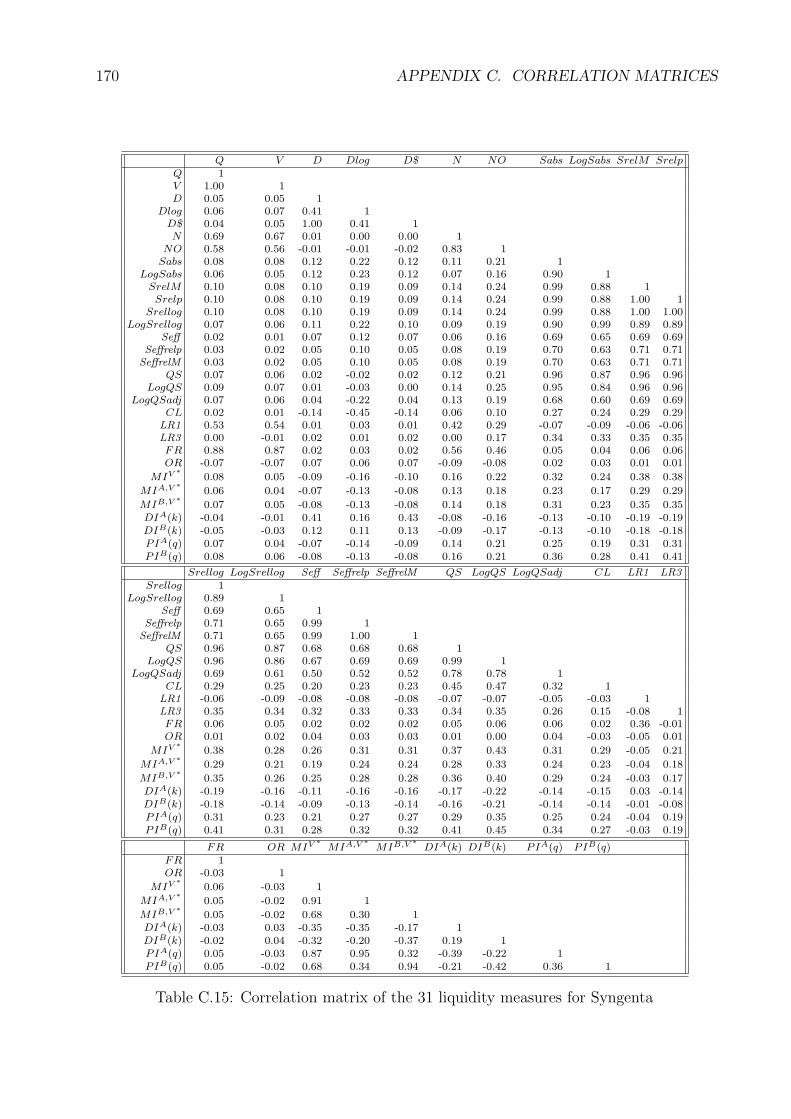
170 APPENDIX C. CORRELATION MATRICES
Q V D Dlog D$ N NO Sabs LogSabs SrelM SrelpQ 1V 1.00 1D 0.05 0.05 1
Dlog 0.06 0.07 0.41 1D$ 0.04 0.05 1.00 0.41 1N 0.69 0.67 0.01 0.00 0.00 1
NO 0.58 0.56 -0.01 -0.01 -0.02 0.83 1Sabs 0.08 0.08 0.12 0.22 0.12 0.11 0.21 1
LogSabs 0.06 0.05 0.12 0.23 0.12 0.07 0.16 0.90 1SrelM 0.10 0.08 0.10 0.19 0.09 0.14 0.24 0.99 0.88 1Srelp 0.10 0.08 0.10 0.19 0.09 0.14 0.24 0.99 0.88 1.00 1
Srellog 0.10 0.08 0.10 0.19 0.09 0.14 0.24 0.99 0.88 1.00 1.00LogSrellog 0.07 0.06 0.11 0.22 0.10 0.09 0.19 0.90 0.99 0.89 0.89
Seff 0.02 0.01 0.07 0.12 0.07 0.06 0.16 0.69 0.65 0.69 0.69Seffrelp 0.03 0.02 0.05 0.10 0.05 0.08 0.19 0.70 0.63 0.71 0.71
SeffrelM 0.03 0.02 0.05 0.10 0.05 0.08 0.19 0.70 0.63 0.71 0.71QS 0.07 0.06 0.02 -0.02 0.02 0.12 0.21 0.96 0.87 0.96 0.96
LogQS 0.09 0.07 0.01 -0.03 0.00 0.14 0.25 0.95 0.84 0.96 0.96LogQSadj 0.07 0.06 0.04 -0.22 0.04 0.13 0.19 0.68 0.60 0.69 0.69
CL 0.02 0.01 -0.14 -0.45 -0.14 0.06 0.10 0.27 0.24 0.29 0.29LR1 0.53 0.54 0.01 0.03 0.01 0.42 0.29 -0.07 -0.09 -0.06 -0.06LR3 0.00 -0.01 0.02 0.01 0.02 0.00 0.17 0.34 0.33 0.35 0.35FR 0.88 0.87 0.02 0.03 0.02 0.56 0.46 0.05 0.04 0.06 0.06OR -0.07 -0.07 0.07 0.06 0.07 -0.09 -0.08 0.02 0.03 0.01 0.01
MIV ∗ 0.08 0.05 -0.09 -0.16 -0.10 0.16 0.22 0.32 0.24 0.38 0.38
MIA,V ∗ 0.06 0.04 -0.07 -0.13 -0.08 0.13 0.18 0.23 0.17 0.29 0.29
MIB,V ∗ 0.07 0.05 -0.08 -0.13 -0.08 0.14 0.18 0.31 0.23 0.35 0.35DIA(k) -0.04 -0.01 0.41 0.16 0.43 -0.08 -0.16 -0.13 -0.10 -0.19 -0.19DIB(k) -0.05 -0.03 0.12 0.11 0.13 -0.09 -0.17 -0.13 -0.10 -0.18 -0.18PIA(q) 0.07 0.04 -0.07 -0.14 -0.09 0.14 0.21 0.25 0.19 0.31 0.31PIB(q) 0.08 0.06 -0.08 -0.13 -0.08 0.16 0.21 0.36 0.28 0.41 0.41
Srellog LogSrellog Seff Seffrelp SeffrelM QS LogQS LogQSadj CL LR1 LR3Srellog 1
LogSrellog 0.89 1Seff 0.69 0.65 1
Seffrelp 0.71 0.65 0.99 1SeffrelM 0.71 0.65 0.99 1.00 1
QS 0.96 0.87 0.68 0.68 0.68 1LogQS 0.96 0.86 0.67 0.69 0.69 0.99 1
LogQSadj 0.69 0.61 0.50 0.52 0.52 0.78 0.78 1CL 0.29 0.25 0.20 0.23 0.23 0.45 0.47 0.32 1
LR1 -0.06 -0.09 -0.08 -0.08 -0.08 -0.07 -0.07 -0.05 -0.03 1LR3 0.35 0.34 0.32 0.33 0.33 0.34 0.35 0.26 0.15 -0.08 1FR 0.06 0.05 0.02 0.02 0.02 0.05 0.06 0.06 0.02 0.36 -0.01OR 0.01 0.02 0.04 0.03 0.03 0.01 0.00 0.04 -0.03 -0.05 0.01
MIV ∗ 0.38 0.28 0.26 0.31 0.31 0.37 0.43 0.31 0.29 -0.05 0.21
MIA,V ∗ 0.29 0.21 0.19 0.24 0.24 0.28 0.33 0.24 0.23 -0.04 0.18
MIB,V ∗ 0.35 0.26 0.25 0.28 0.28 0.36 0.40 0.29 0.24 -0.03 0.17DIA(k) -0.19 -0.16 -0.11 -0.16 -0.16 -0.17 -0.22 -0.14 -0.15 0.03 -0.14DIB(k) -0.18 -0.14 -0.09 -0.13 -0.14 -0.16 -0.21 -0.14 -0.14 -0.01 -0.08PIA(q) 0.31 0.23 0.21 0.27 0.27 0.29 0.35 0.25 0.24 -0.04 0.19PIB(q) 0.41 0.31 0.28 0.32 0.32 0.41 0.45 0.34 0.27 -0.03 0.19
FR OR MIV ∗ MIA,V ∗ MIB,V ∗ DIA(k) DIB(k) PIA(q) PIB(q)FR 1OR -0.03 1
MIV ∗ 0.06 -0.03 1
MIA,V ∗ 0.05 -0.02 0.91 1
MIB,V ∗ 0.05 -0.02 0.68 0.30 1DIA(k) -0.03 0.03 -0.35 -0.35 -0.17 1DIB(k) -0.02 0.04 -0.32 -0.20 -0.37 0.19 1PIA(q) 0.05 -0.03 0.87 0.95 0.32 -0.39 -0.22 1PIB(q) 0.05 -0.02 0.68 0.34 0.94 -0.21 -0.42 0.36 1
Table C.15: Correlation matrix of the 31 liquidity measures for Syngenta
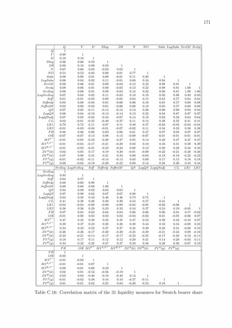
171
Q V D Dlog D$ N NO Sabs LogSabs SrelM SrelpQ 1V 0.99 1D 0.10 0.10 1
Dlog 0.06 0.06 0.59 1D$ 0.09 0.10 0.99 0.59 1N 0.67 0.66 0.03 -0.03 0.02 1
NO 0.54 0.53 0.03 0.00 0.01 0.77 1Sabs 0.08 0.06 0.01 0.09 -0.01 0.11 0.20 1
LogSabs 0.06 0.04 0.02 0.11 -0.01 0.08 0.16 0.94 1SrelM 0.09 0.06 0.01 0.09 -0.03 0.12 0.22 0.98 0.91 1Srelp 0.09 0.06 0.01 0.09 -0.03 0.12 0.22 0.98 0.91 1.00 1
Srellog 0.09 0.06 0.01 0.09 -0.03 0.12 0.22 0.98 0.91 1.00 1.00LogSrellog 0.07 0.04 0.02 0.11 -0.03 0.10 0.19 0.92 0.98 0.93 0.93
Seff 0.01 -0.01 -0.03 0.00 -0.05 0.04 0.15 0.64 0.57 0.64 0.64Seffrelp 0.03 0.00 -0.03 0.01 -0.06 0.06 0.18 0.65 0.57 0.68 0.68
SeffrelM 0.03 0.00 -0.03 0.01 -0.06 0.06 0.18 0.65 0.57 0.68 0.68QS 0.07 0.05 -0.11 -0.14 -0.13 0.12 0.20 0.96 0.90 0.94 0.94
LogQS 0.08 0.04 -0.10 -0.13 -0.14 0.13 0.22 0.94 0.87 0.97 0.97LogQSadj 0.07 0.05 -0.04 -0.34 -0.07 0.14 0.18 0.62 0.56 0.64 0.64
CL 0.02 -0.01 -0.25 -0.49 -0.27 0.11 0.14 0.38 0.35 0.41 0.41LR1 0.70 0.72 0.11 0.07 0.11 0.49 0.37 -0.02 -0.03 -0.04 -0.04LR3 -0.01 -0.03 -0.04 -0.01 -0.07 -0.02 0.11 0.34 0.33 0.38 0.38FR 0.86 0.86 0.06 0.03 0.06 0.61 0.47 0.07 0.05 0.07 0.07OR -0.07 -0.07 0.13 0.08 0.13 -0.09 -0.07 -0.01 -0.01 -0.01 -0.01
MIV ∗ -0.01 -0.05 -0.23 -0.28 -0.27 0.05 0.14 0.40 0.37 0.47 0.47
MIA,V ∗ -0.01 -0.04 -0.17 -0.21 -0.20 0.02 0.10 0.33 0.31 0.39 0.39
MIB,V ∗ -0.01 -0.03 -0.21 -0.23 -0.24 0.06 0.12 0.30 0.28 0.34 0.34DIA(k) 0.02 0.05 0.17 0.19 0.20 -0.01 -0.09 -0.22 -0.21 -0.26 -0.26DIB(k) 0.07 0.08 0.31 0.21 0.33 0.00 -0.03 -0.19 -0.18 -0.22 -0.22PIA(q) -0.01 -0.02 -0.11 -0.14 -0.13 0.03 0.09 0.17 0.15 0.18 0.18PIB(q) 0.00 -0.02 -0.19 -0.20 -0.22 0.09 0.14 0.28 0.26 0.34 0.34
Srellog LogSrellog Seff Seffrelp SeffrelM QS LogQS LogQSadj CL LR1 LR3Srellog 1
LogSrellog 0.93 1Seff 0.64 0.57 1
Seffrelp 0.68 0.60 0.98 1SeffrelM 0.68 0.60 0.98 1.00 1
QS 0.94 0.89 0.62 0.63 0.63 1LogQS 0.97 0.90 0.62 0.67 0.67 0.98 1
LogQSadj 0.64 0.58 0.43 0.46 0.46 0.73 0.75 1CL 0.41 0.38 0.26 0.30 0.30 0.54 0.57 0.41 1
LR1 -0.04 -0.04 -0.09 -0.09 -0.09 -0.04 -0.05 -0.02 -0.06 1LR3 0.38 0.36 0.29 0.33 0.33 0.34 0.37 0.24 0.19 -0.05 1FR 0.07 0.05 0.03 0.04 0.04 0.06 0.06 0.06 0.01 0.57 -0.02OR -0.01 0.00 0.03 0.03 0.03 -0.03 -0.02 0.01 -0.05 -0.06 0.07
MIV ∗ 0.47 0.45 0.29 0.35 0.35 0.47 0.53 0.39 0.42 -0.10 0.27
MIA,V ∗ 0.39 0.37 0.23 0.28 0.28 0.39 0.44 0.33 0.34 -0.09 0.23
MIB,V ∗ 0.34 0.33 0.23 0.27 0.27 0.35 0.39 0.28 0.31 -0.08 0.19DIA(k) -0.26 -0.26 -0.17 -0.20 -0.20 -0.25 -0.29 -0.21 -0.24 0.09 -0.16DIB(k) -0.22 -0.21 -0.14 -0.17 -0.17 -0.23 -0.25 -0.17 -0.20 0.10 -0.14PIA(q) 0.18 0.17 0.11 0.12 0.12 0.20 0.21 0.14 0.20 -0.03 0.11PIB(q) 0.34 0.32 0.22 0.27 0.27 0.33 0.38 0.28 0.30 -0.07 0.19
FR OR MIV ∗ MIA,V ∗ MIB,V ∗ DIA(k) DIB(k) PIA(q) PIB(q)FR 1OR -0.03 1
MIV ∗ -0.01 -0.02 1
MIA,V ∗ -0.01 -0.01 0.87 1
MIB,V ∗ 0.00 -0.01 0.68 0.23 1DIA(k) 0.02 0.01 -0.52 -0.56 -0.19 1DIB(k) 0.03 0.03 -0.40 -0.19 -0.49 0.13 1PIA(q) -0.01 -0.02 0.38 0.44 0.10 -0.37 -0.11 1PIB(q) 0.01 -0.01 0.62 0.25 0.84 -0.20 -0.53 0.10 1
Table C.16: Correlation matrix of the 31 liquidity measures for Swatch bearer share
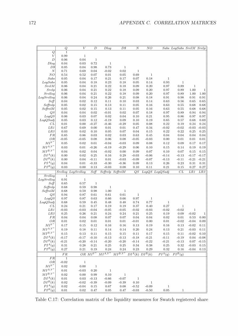
172 APPENDIX C. CORRELATION MATRICES
Q V D Dlog D$ N NO Sabs LogSabs SrelM SrelpQ 1V 0.99 1D 0.06 0.04 1
Dlog 0.04 0.03 0.72 1D$ 0.05 0.04 0.98 0.73 1N 0.71 0.69 0.04 -0.02 0.02 1
NO 0.54 0.52 0.07 0.01 0.05 0.69 1Sabs 0.05 0.04 0.17 0.21 0.17 0.07 0.18 1
LogSabs 0.05 0.04 0.18 0.23 0.18 0.05 0.14 0.93 1SrelM 0.06 0.04 0.21 0.22 0.18 0.09 0.20 0.97 0.89 1Srelp 0.06 0.04 0.21 0.22 0.18 0.09 0.20 0.97 0.89 1.00 1
Srellog 0.06 0.04 0.21 0.22 0.18 0.09 0.20 0.97 0.89 1.00 1.00LogSrellog 0.06 0.04 0.24 0.26 0.21 0.08 0.18 0.91 0.98 0.91 0.91
Seff 0.04 0.02 0.12 0.11 0.10 0.03 0.14 0.63 0.56 0.65 0.65Seffrelp 0.05 0.02 0.15 0.13 0.11 0.05 0.16 0.63 0.55 0.68 0.68
SeffrelM 0.05 0.02 0.15 0.13 0.11 0.05 0.16 0.63 0.55 0.68 0.68QS 0.04 0.04 0.02 -0.01 0.02 0.07 0.18 0.97 0.89 0.94 0.94
LogQS 0.06 0.03 0.07 0.02 0.04 0.10 0.21 0.95 0.86 0.97 0.97LogQSadj 0.05 0.03 0.12 -0.19 0.09 0.10 0.19 0.65 0.57 0.68 0.69
CL 0.01 0.00 -0.27 -0.46 -0.29 0.05 0.08 0.22 0.19 0.24 0.24LR1 0.67 0.69 0.00 0.01 0.01 0.47 0.34 -0.02 -0.02 -0.03 -0.03LR3 0.03 0.02 0.10 0.05 0.07 0.04 0.15 0.22 0.22 0.25 0.25FR 0.85 0.86 0.03 0.02 0.03 0.63 0.45 0.04 0.04 0.04 0.04OR -0.05 -0.05 0.08 0.06 0.08 -0.05 -0.03 0.00 0.01 0.01 0.01
MIV ∗ 0.05 0.02 0.01 -0.04 -0.03 0.09 0.08 0.12 0.09 0.17 0.17
MIA,V ∗ 0.03 0.01 -0.26 -0.19 -0.29 0.06 0.10 0.15 0.14 0.19 0.19
MIB,V ∗ 0.04 0.02 0.04 -0.02 0.00 0.09 0.07 0.10 0.07 0.15 0.15DIA(k) 0.00 0.02 0.25 0.16 0.29 -0.03 -0.06 -0.14 -0.13 -0.17 -0.17DIB(k) 0.00 0.04 -0.11 0.01 -0.03 -0.09 -0.07 -0.13 -0.11 -0.21 -0.21PIA(q) 0.04 0.01 -0.33 -0.30 -0.36 0.09 0.13 0.26 0.23 0.31 0.31PIB(q) 0.03 0.00 0.13 -0.03 0.08 0.10 0.11 0.21 0.15 0.27 0.27
Srellog LogSrellog Seff Seffrelp SeffrelM QS LogQS LogQSadj CL LR1 LR3Srellog 1
LogSrellog 0.91 1Seff 0.65 0.57 1
Seffrelp 0.68 0.59 0.98 1SeffrelM 0.68 0.59 0.98 1.00 1
QS 0.94 0.87 0.61 0.61 0.61 1LogQS 0.97 0.87 0.63 0.66 0.66 0.97 1
LogQSadj 0.68 0.59 0.45 0.48 0.48 0.74 0.77 1CL 0.24 0.21 0.17 0.19 0.19 0.37 0.40 0.27 1
LR1 -0.03 -0.03 -0.04 -0.05 -0.05 -0.02 -0.03 -0.02 -0.02 1LR3 0.25 0.26 0.21 0.24 0.24 0.21 0.25 0.19 0.09 -0.02 1FR 0.04 0.04 0.08 0.07 0.07 0.04 0.04 0.02 0.01 0.53 0.00OR 0.01 0.02 0.01 0.01 0.01 -0.01 0.00 0.01 -0.02 -0.04 0.09
MIV ∗ 0.17 0.15 0.12 0.16 0.16 0.13 0.19 0.16 0.13 -0.02 0.11
MIA,V ∗ 0.19 0.18 0.11 0.14 0.14 0.20 0.24 0.13 0.21 -0.03 0.11
MIB,V ∗ 0.15 0.13 0.11 0.15 0.15 0.11 0.17 0.15 0.11 -0.02 0.10DIA(k) -0.17 -0.17 -0.10 -0.13 -0.13 -0.18 -0.21 -0.11 -0.19 0.04 -0.08DIB(k) -0.21 -0.20 -0.14 -0.20 -0.20 -0.14 -0.22 -0.21 -0.13 0.07 -0.15PIA(q) 0.31 0.28 0.21 0.25 0.25 0.34 0.38 0.25 0.32 -0.03 0.15PIB(q) 0.27 0.21 0.19 0.24 0.24 0.23 0.29 0.32 0.16 -0.04 0.13
FR OR MIV ∗ MIA,V ∗ MIB,V ∗ DIA(k) DIB(k) PIA(q) PIB(q)FR 1OR -0.02 1
MIV ∗ 0.02 0.00 1
MIA,V ∗ 0.01 -0.03 0.20 1
MIB,V ∗ 0.02 0.00 0.99 0.10 1DIA(k) 0.01 0.03 -0.13 -0.66 -0.07 1DIB(k) 0.02 -0.02 -0.39 -0.09 -0.39 0.10 1PIA(q) 0.02 -0.04 0.15 0.67 0.08 -0.52 -0.09 1PIB(q) 0.01 0.02 0.47 0.05 0.47 -0.03 -0.50 0.05 1
Table C.17: Correlation matrix of the liquidity measures for Swatch registered share

173
Q V D Dlog D$ N NO Sabs LogSabs SrelM SrelpQ 1V 0.99 1D 0.09 0.10 1
Dlog 0.05 0.06 0.72 1D$ 0.08 0.10 0.99 0.71 1N 0.74 0.72 0.00 -0.03 -0.01 1
NO 0.46 0.44 -0.04 -0.06 -0.05 0.61 1Sabs 0.06 0.05 0.03 0.11 0.01 0.07 0.22 1
LogSabs 0.04 0.03 0.03 0.13 0.01 0.03 0.20 0.90 1SrelM 0.06 0.04 0.00 0.07 -0.04 0.09 0.23 0.98 0.87 1Srelp 0.06 0.04 0.00 0.07 -0.04 0.09 0.23 0.98 0.87 1.00 1
Srellog 0.06 0.04 0.00 0.07 -0.04 0.09 0.23 0.98 0.87 1.00 1.00LogSrellog 0.05 0.02 0.00 0.10 -0.04 0.06 0.22 0.89 0.98 0.89 0.89
Seff 0.00 -0.01 -0.07 -0.04 -0.09 0.03 0.17 0.57 0.46 0.57 0.57Seffrelp 0.01 -0.01 -0.08 -0.05 -0.11 0.05 0.19 0.58 0.46 0.61 0.60
SeffrelM 0.01 -0.01 -0.08 -0.05 -0.11 0.05 0.19 0.58 0.46 0.61 0.61QS 0.05 0.04 -0.14 -0.17 -0.16 0.08 0.24 0.94 0.85 0.93 0.93
LogQS 0.06 0.03 -0.15 -0.18 -0.19 0.10 0.25 0.92 0.82 0.95 0.95LogQSadj 0.05 0.03 -0.08 -0.36 -0.10 0.09 0.19 0.59 0.53 0.62 0.62
CL 0.04 0.01 -0.32 -0.49 -0.33 0.09 0.16 0.34 0.29 0.38 0.38LR1 0.69 0.71 0.10 0.07 0.11 0.49 0.26 -0.02 -0.02 -0.03 -0.03LR3 0.06 0.04 -0.06 -0.06 -0.08 0.07 0.20 0.24 0.23 0.26 0.26FR 0.83 0.84 0.05 0.03 0.05 0.66 0.39 0.03 0.02 0.03 0.03OR -0.07 -0.07 0.11 0.06 0.11 -0.08 -0.05 -0.01 -0.01 -0.02 -0.02
MIV ∗ 0.01 -0.02 -0.16 -0.17 -0.19 0.09 0.17 0.22 0.18 0.29 0.29
MIA,V ∗ -0.02 -0.04 -0.14 -0.14 -0.17 0.05 0.10 0.16 0.14 0.22 0.22
MIB,V ∗ 0.01 -0.01 -0.13 -0.14 -0.16 0.08 0.15 0.19 0.16 0.25 0.25DIA(k) 0.06 0.09 0.25 0.21 0.29 -0.04 -0.11 -0.19 -0.20 -0.24 -0.25DIB(k) 0.05 0.08 0.29 0.22 0.33 -0.06 -0.12 -0.19 -0.19 -0.25 -0.25PIA(q) -0.04 -0.06 -0.15 -0.15 -0.18 0.03 0.09 0.12 0.10 0.17 0.17PIB(q) -0.02 -0.05 -0.22 -0.20 -0.26 0.07 0.15 0.25 0.22 0.32 0.32
Srellog LogSrellog Seff Seffrelp SeffrelM QS LogQS LogQSadj CL LR1 LR3Srellog 1
LogSrellog 0.89 1Seff 0.57 0.47 1
Seffrelp 0.61 0.49 0.99 1SeffrelM 0.61 0.49 0.99 1.00 1
QS 0.93 0.85 0.57 0.58 0.58 1LogQS 0.95 0.85 0.56 0.60 0.60 0.98 1
LogQSadj 0.62 0.55 0.37 0.40 0.40 0.73 0.75 1CL 0.38 0.33 0.25 0.28 0.28 0.55 0.59 0.39 1
LR1 -0.03 -0.04 -0.06 -0.07 -0.07 -0.03 -0.04 -0.02 -0.04 1LR3 0.26 0.25 0.22 0.24 0.24 0.25 0.27 0.19 0.15 0.00 1FR 0.03 0.02 0.01 0.01 0.01 0.03 0.02 0.02 0.02 0.57 0.01OR -0.02 -0.02 0.00 -0.01 -0.01 -0.03 -0.03 0.01 -0.04 -0.05 0.02
MIV ∗ 0.29 0.26 0.20 0.25 0.25 0.28 0.34 0.25 0.29 -0.06 0.16
MIA,V ∗ 0.22 0.21 0.11 0.16 0.16 0.19 0.25 0.17 0.20 -0.07 0.11
MIB,V ∗ 0.25 0.22 0.18 0.22 0.22 0.24 0.30 0.22 0.26 -0.05 0.14DIA(k) -0.24 -0.27 -0.16 -0.20 -0.20 -0.24 -0.28 -0.19 -0.21 0.12 -0.12DIB(k) -0.25 -0.26 -0.16 -0.20 -0.20 -0.24 -0.29 -0.19 -0.22 0.11 -0.15PIA(q) 0.17 0.16 0.09 0.13 0.12 0.16 0.20 0.13 0.17 -0.07 0.08PIB(q) 0.32 0.31 0.21 0.27 0.27 0.29 0.36 0.24 0.29 -0.10 0.17
FR OR MIV ∗ MIA,V ∗ MIB,V ∗ DIA(k) DIB(k) PIA(q) PIB(q)FR 1OR -0.03 1
MIV ∗ -0.01 -0.03 1
MIA,V ∗ -0.02 -0.01 0.35 1
MIB,V ∗ 0.00 -0.02 0.97 0.10 1DIA(k) 0.05 0.04 -0.27 -0.39 -0.19 1DIB(k) 0.05 0.04 -0.38 -0.20 -0.34 0.30 1PIA(q) -0.03 -0.02 0.30 0.81 0.10 -0.46 -0.20 1PIB(q) -0.02 -0.04 0.72 0.21 0.71 -0.33 -0.64 0.21 1
Table C.18: Correlation matrix of the 31 liquidity measures for Unaxis

174 APPENDIX C. CORRELATION MATRICES

Abbreviations
Abbreviation Description
ACD autoregressive conditional duration
a.m. before noon
AMEX American Stock Exchange
B buy
CHF Swiss Franc
CP counterparty
Cpty counterparty
ECN electronic communications network
e.g. for example
et al. and others
ETHZ Eidgenossische Technische Hochschule Zurich
f. following page
ff. following pages
FX foreign exchange
ID identification
mio. million
N nostro
NASDAQ North American Security Dealers Automated Quotation System
Norm normal
NYSE New York Stock Exchange
OH order history
OHR order history report
OTC Over the counter
p. page
PCA principal component analysis
p.m. afternoon
Rnd round
SIA Securities Industry Association
SMI Swiss Market Index
Std. Dev. standard deviation
SWX Swiss Exchange
U.S. United States
USD United States Dollar
VAR vector autoregression
175

176 ABBREVIATIONS

Ticker Symbols of the Stocks used
Ticker StockADEN AdeccoBAER Julius BaerCFR RichemontCIBN CibaCLN ClariantGIVN GivaudanHOLN HolcimKUD KudelskiLONN LonzaRUKN Swiss ReSCMN SwisscomSEO SeronoSGSN SurveillanceSUN SulzerSYNN SyngentaUHR Swatch baerer shareUHRN Swatch registered shareUNAX Unaxis
177

178 TICKER SYMBOLS
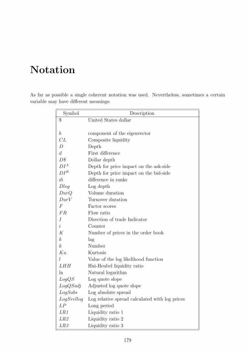
Notation
As far as possible a single coherent notation was used. Nevertheless, sometimes a certain
variable may have different meanings.
Symbol Description
$ United States dollar
b component of the eigenvector
CL Composite liquidity
D Depth
d First difference
D$ Dollar depth
DIA Depth for price impact on the ask-side
DIB Depth for price impact on the bid-side
di difference in ranks
Dlog Log depth
DurQ Volume duration
DurV Turnover duration
F Factor scores
FR Flow ratio
I Direction of trade Indicator
i Counter
K Number of prices in the order book
k lag
k Number
Ku Kurtosis
l Value of the log likelihood function
LHH Hui-Heubel liquidity ratio
ln Natural logarithm
LogQS Log quote slope
LogQSadj Adjusted log quote slope
LogSabs Log absolute spread
LogSrellog Log relative spread calculated with log prices
LP Long period
LR1 Liquidity ratio 1
LR2 Liquidity ratio 2
LR3 Liquidity ratio 3
179
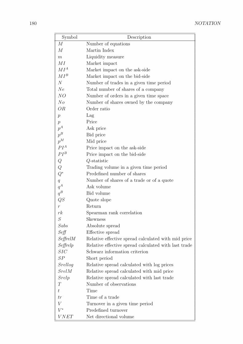
180 NOTATION
Symbol Description
M Number of equations
M Martin Index
m Liquidity measure
MI Market impact
MIA Market impact on the ask-side
MIB Market impact on the bid-side
N Number of trades in a given time period
Ne Total number of shares of a company
NO Number of orders in a given time space
No Number of shares owned by the company
OR Order ratio
p Lag
p Price
pA Ask price
pB Bid price
pM Mid price
PIA Price impact on the ask-side
PIB Price impact on the bid-side
Q Q-statistic
Q Trading volume in a given time period
Q∗ Predefined number of shares
q Number of shares of a trade or of a quote
qA Ask volume
qB Bid volume
QS Quote slope
r Return
rk Spearman rank correlation
S Skewness
Sabs Absolute spread
Seff Effective spread
SeffrelM Relative effective spread calculated with mid price
Seffrelp Relative effective spread calculated with last trade
SIC Schwarz information criterion
SP Short period
Srellog Relative spread calculated with log prices
SrelM Relative spread calculated with mid price
Srelp Relative spread calculated with last trade
T Number of observations
t Time
tr Time of a trade
V Turnover in a given time period
V ∗ Predefined turnover
V NET Net directional volume
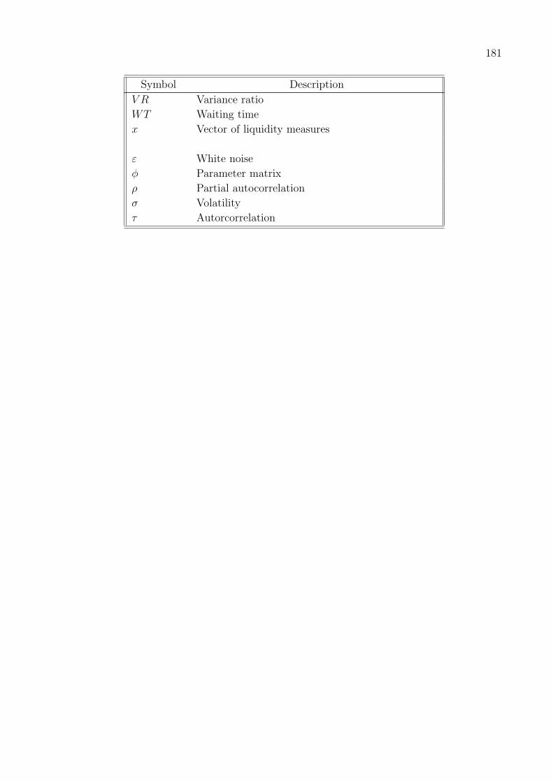
181
Symbol Description
V R Variance ratio
WT Waiting time
x Vector of liquidity measures
ε White noise
φ Parameter matrix
ρ Partial autocorrelation
σ Volatility
τ Autorcorrelation

182 NOTATION

Bibliography
Acker, D., Stalker, M. & Tonks, I. (2002), ‘Daily closing inside spreads and trading vol-
umes around earnings announcements’, Journal of Business Finance & Accounting
29(9/10), 1149–1179.
Amihud, Y. (2002), ‘Illiquidity and stock returns: Cross-section and time-series effects’,
Journal of Financial Markets 5, 31–56.
Amihud, Y. & Mendelson, H. (1991), ‘Liquidity, maturity and the yields on U.S. Treasury
securities’, Journal of Finance 46(4), 1411–1425.
Andersen, T. G. & Bollerslev, T. (1997), ‘Intraday periodicity and volatility persistence in
financial markets’, Journal of Empirical Finance 4(2-3), 115–158.
Andersen, T. G. & Bollerslev, T. (1998), ‘Deutsche mark-dollar volatility: Intraday activity
patterns, macroeconomic announcements and longer run dependencies.’, The Journal
of Finance 53(1), 219–265.
Bacidore, J. M. (1997), ‘The impact of decimalization on market quality: An empirical inves-
tigation of the Toronto stock exchange’, Journal of Financial Intermediation 6(2), 92–
120.
Bacidore, J. M., Battalio, R. H. & Jennings, R. H. (2002), ‘Depth improvement and adjusted
price improvement on the New York Stock Exchange’, Journal of Financial Markets
5, 169–195.
Baillie, R. T. & Dacorogna, M. M. (1997), ‘High frequency data in finance’, Journal of
Empirical Finance 4(2-3), 69–72.
Baker, H. K. (1996), ‘Trading location and liquidity: An analysis of U.S. dealer and agency
markets for comon stocks’, Financial Markets, Institutions & Instruments 5(4), 1–51.
Ball, C. A. & Chordia, T. (2001), ‘True spreads and equilibrium prices’, The Journal of
Finance 56(5), 1801–1835.
Barclay, M. J., Christie, W. G., Harris, J. H., Kandel, E. & Schultz, P. H. (1999), ‘Effects
of market reform on the trading costs and depths of NASDAQ stocks’, The Journal of
Finance 54(1), 1–34.
Battalio, R., Greene, J. & Jennings, R. (1998), ‘Order flow distribution, bid-ask spreads,
and liquidity costs: Merril Lynch’s decision to cease routinely routing orders to regional
stock exchanges’, Journal of Financial Intermediation 7, 338–358.
183

184 BIBLIOGRAPHY
Box, G. E. P. & Jenkins, G. M. (1976), Time Series Analysis, Forecasting and Control,
Holden-Day, San Francisco.
Breedon, F. & Holland, A. (1997), Electronic versus open outcry markets: The case of the
Bund futures contract. Working Paper, Bank of England.
Brockman, P. & Chung, D. Y. (2000), ‘An empirical investigation of trading on asymmetric
information and heterogeneous prior beliefs’, Journal of Empirical Finance 7, 417–454.
Brunner, A. (1996), ‘Messkonzepte zur Liquiditat auf Wertpapiermarkten’. Beitrage zur
Theorie der Finanzmarkte, Universitat Frankfurt.
Butler, A. W., Grullon, G. & Weston, J. P. (2002), Stock market liquidity and the cost of
raising capital. Working Paper.
Campbell, J. Y., Lo, A. & MacKinlay, C. (1997), The Econometrics of Financial Markets,
Princeton University Press, Princeton.
Chan, H. W.-H. & Pinder, S. M. (2000), ‘The value of liquidity: Evidence from the derivatives
market’, Pacific-Basin Finance Journal 8, 483–503.
Chan, K., Chung, Y. P. & Fong, W.-M. (2002), ‘The informational role of stock and option
volume’, The Review of Financial Studies 15(4), 1049–1075.
Chordia, T., Roll, R. & Subrahmanyam, A. (2000), ‘Commonality in liquidity’, Journal of
Financial Economics 56, 3–28.
Chordia, T., Roll, R. & Subrahmanyam, A. (2001), ‘Market liquidity and trading activity’,
The Journal of Finance 56(2), 501–530.
Chordia, T., Subrahmanyam, A. & Anshuman, V. R. (2001), ‘Trading activity and expected
stock returns’, Journal of Financial Economics 59, 3–32.
Chordia, T. & Swaminathan, B. (2000), ‘Trading volume and cross-autocorrelations in stock
returns’, The Journal of Finance 55(2), 913–935.
Christie, W. G. & Schultz, P. H. (1998), ‘Dealer markets under stress: The performance
of NASDAQ market makers during the november 15, 1991, market break’, Journal of
Finacial Services Research 13(3), 205–229.
Chung, K. H., Van Ness, B. F. & Van Ness, R. A. (1999), ‘Limit orders and the bid-ask
spread’, Journal of Financial Economics 53, 255–287.
Chung, K. H. & Van Ness, R. A. (2001), ‘Order handling rules, tick size, and the intraday
pattern of bid-ask spreads for NASDAQ stocks’, Journal of Financial Markets 4, 143–
161.
Chung, M. M. C., Han, K. C. & Tse, M. K. S. (1996), ‘Interrelationship among the price in-
dexes of the NYSE, AMEX and OTC’, International Review of Economics and Finance
5(1), 63–75.
BIBLIOGRAPHY 185
Clyman, D. R., Allen, C. S. & Jaycobs, R. (1997), ‘Liquidity without volume: The case of
FINEX, Dublin’, The Journal of Futures Markets 17(3), 247–277.
Clyman, D. R. & Jaycobs, R. (1998), ‘Liquidity without volume. II. using block orders to
measure market resiliency’, The Journal of Futures Markets 18(3), 281–296.
Coppejans, M. & Domowitz, I. (2002), An empirical analysis of trades, orders, and cancel-
lations in a limit order market. Working Paper.
Coppejans, M., Domowitz, I. & Madhavan, A. (2003), Resiliency in an automated auction.
Working Paper.
Corwin, S. A. (1999), ‘Differences in trading behavior across NYSE specialist firms’, The
Journal of Finance 54(2), 721–745.
Corwin, S. A. & Lipson, M. L. (2000), ‘Order flow and liquidity around NYSE trading halts’,
The Journal of Finance 55(4), 1771–1805.
Dacorogna, M. M., Gencay, R., Muller, U., Olsen, R. B. & Pictet, O. V. (2001), An Intro-
duction to High-Frequency Finance, Academic Press, San Diego.
Danıelsson, J. & Payne, R. (2002), ‘Real trading patterns and prices in spot foreign exchange
markets’, Journal of International Money and Finance 21, 203–222.
Elyasiani, E., Hauser, S. & Lauterbach, B. (2000), ‘Market response to liquidity improve-
ments: Evidence from exchange listings’, The Financial Review 41, 1–14.
Engle, R. F. & Lange, J. (2001), ‘Predicting VNET: A model of the dynamics of market
depth’, Journal of Financial Markets 4, 113–142.
Fernandez, F. A. (1999), Liquidity risk. SIA Working Paper.
Fleming, M. J. & Remolona, E. M. (1999), ‘Price formation and liquidity in the U.S. Treasury
market: The response to public information’, The Journal of Finance 54(5), 1901–1915.
George, T. J. & Hwang, C.-Y. (1998), ‘Endogenous market statistics and security pricing:
An empirical investigation’, Journal of Financial Markets 1, 285–319.
Gervais, S., Kaniel, R. & Mingelgrin, D. H. (2001), ‘The high-volume return premium’, The
Journal of Finance 56(3), 877–919.
Goldstein, M. A. & Kavajecz, K. A. (2000), ‘Eighths, sixteenths and market depth: Changes
in tick size and liquidity provision on the NYSE’, Journal of Financial Economics
56, 125–149.
Gomber, P. & Schweickert, U. (2002), ‘Der Market Impact: Liquiditatsmass im elektronis-
chen Wertpapierhandel’, Die Bank 7, 485–489.
Gourieroux, C., Jasiak, J. & Le Fol, G. (1999), ‘Intra-day market activity’, Journal of
Financial Markets 2, 193–226.

186 BIBLIOGRAPHY
Grammig, J., Schiereck, D. & Theissen, E. (2001), ‘Knowing me, knowing you: Trader
anonymity and informed trading in parallel markets’, Journal of Financial Markets
4, 385–412.
Greene, J. & Smart, S. (1999), ‘Liquidity provision and noise trading: Evidence from the
“investment dartboard” column’, The Journal of Finance 54(5), 1885–1899.
Gwilym, O. A. & Sutcliffe, C. (1999), High-Frequency Financial Market Data, Risk Books,
London.
Hamao, Y. & Hasbrouck, J. (1995), ‘Securities trading in the absence of dealers: Trades and
quotes on the Tokyo Stock Exchange’, The Review of Financial Studies 8(3), 849–878.
Hamilton, J. D. (1994), Time Series Analysis, Princeton University Press, Princeton.
Harris, F. H. d., McInish, T. H. & Wood, R. A. (2002), ‘Security price adjustment across
exchanges: An investigation of common factor components for Dow stocks’, Journal of
Financial Markets 5(3), 277–308. Working Paper.
Hasbrouck, J. (1999), ‘The dynamics of discrete bid and ask quotes’, The Journal of Finance
54(6), 2109–2142.
Hasbrouck, J. (2003), Intraday price formation in U.S. equity index markets. forthcoming
in the Journal of Finance, December.
Hasbrouck, J. & Saar, G. (2002), Limit orders and volatility in a hybrid market: The Island
ECN. Working Paper.
Hasbrouck, J. & Seppi, D. J. (2001), ‘Common factors in prices, order flows and liquidity’,
Journal of Financial Economics 59, 383–411.
Hotelling, H. (1933), ‘Analysis of a complex of statistical varables into principal components’,
Journal of Educational Psychology 24, 417–441,498–520.
Huberman, G. & Halka, D. (2001), ‘Systematic liquidity’, The Journal of Financial Research
24(2), 161–178.
Irvine, P., Benston, G. & Kandel, E. (2000), Liquidity beyond the inside spread: Measuring
and using information in the limit order book. Working Paper.
Ito, T., Lyons, R. K. & Melvin, M. T. (1998), ‘Is there private information in the FX market?
The Tokyo experiment’, The Journal of Finance 53(3), 1111–1130.
Jones, C. M. & Lipson, M. L. (1999), Price impacts and quote adjustment on the NASDAQ
and NYSE/AMEX. Working Paper.
Kaiser, H. F. (1958), ‘The varimax criterion of analytic rotation in factor analysis’, Psy-
chometrika 23, 187–200.
Kamara, A. & Koski, J. L. (2001), ‘Volatility, autocorrelations, and trading activity after
stock splits’, Journal of Financial Markets 4, 163–184.
BIBLIOGRAPHY 187
Kanji, G. K. (1999), 100 Statistical Tests, Sage, London.
Karagozoglu, A. K. (2000), Microstructure model of futures markets: Theory and evidence
for optimal hedging strategies. Working Paper.
Kavajecz, K. A. (1999), ‘A specialist’s quoted depth and the limit order book’, The Journal
of Finance 54(2), 747–771.
Kavajecz, K. A. & Odders-White, E. R. (2001), ‘Volatility and market structure’, Journal
of Financial Markets 4, 359–384.
Kluger, B. D. & Stephan, J. (1997), ‘Alternative liquidity measures and stock returns’,
Review of Quantitative Finance and Accounting 8(1), 19–36.
Lee, C. M. C., Mucklow, B. & Ready, M. J. (1993), ‘Spreads, depths and the impact of
earnings information: An intraday analysis’, The Review of Financial Studies 6(2), 345–
374.
Lee, C. M. C. & Swaminathan, B. (2000), ‘Price momentum and trading volume’, The
Journal of Finance 55(5), 2017–2069.
Lee, Y.-T., Fok, R. C. W. & Liu, Y.-J. (2001), ‘Explaining intraday pattern of trading volume
from the order flow data’, Journal of Business Finance & Accounting 28(1), 199–230.
Levin, E. J. & Wright, R. E. (1999), ‘Explaining the intra-day variation in the bid-ask spread
in competitive dealership markets – A research note’, Journal of Financial Markets
2, 179–191.
Lin, J.-C., Sanger, G. C. & Booth, G. G. (1995), ‘Trade size and components of the bid-ask
spread’, The Review of Financial Studies 8(4), 1153–1183.
Ljung, G. M. & Box, G. (1978), ‘On a measure of lack of fit in time series models’, Biometrika
65, 297–303.
Loderer, C. & Roth, L. (2001), The pricing discount for limited liquidity: Evidence from
Switzerland. Working Paper.
Madhavan, A. (2000), ‘Market microstructure: A survey’, Journal of Financial Markets
3, 205–258.
Menyah, K. & Paudyal, K. (2000), ‘The components of bid-ask spreads on the London stock
exchange’, Journal of Banking and Finance 24, 1767–1785.
O’Hara, M. (1995), Market Microstructure Theory, Blackwell, Malden.
Pearson, K. (1901), ‘On lines and planes of closest fit to systems of points in space’, Philo-
sophical Magazine 6(2), 559–572.
Peng, L. (2001), Trading takes time. Working Paper, Yale University.

188 BIBLIOGRAPHY
Ranaldo, A. (2000), Intraday Trading Activity on Financial Markets: The Swiss Evidence,
PhD thesis, University of Fribourg.
Ranaldo, A. (2001), ‘Intraday market liquidity on the Swiss stock exchange’, Financial
Markets and Portfolio Management 15(3), 309–327.
Ranaldo, A. (2002), ‘Transaction costs on the Swiss stock exchange’, Financial Markets and
Portfolio Management 16(1), 53–68.
Ranaldo, A. (2003), Intraday market dynamics around public information arrivals. Working
Paper.
Ranaldo, A. (2004), ‘Order aggressiveness in limit order book markets’, Journal of Financial
Markets 7(1), 53–74.
Sarin, A., Shastri, K. A. & Shastri, K. (1996), Ownership structure and stock market liqudity.
Working Paper, Santa Clara University.
Schoch, J. (2001), Uber das Pricing von Liquiditat auf Aktienmarkten, Master’s thesis,
University of St. Gallen.
Schultz, P. (2000), ‘Stock splits, tick size, and sponsorship’, The Journal of Finance
55(1), 429–451.
Schwarz, G. (1978), ‘Estimating the dimension of a model’, The Annals of Statistics
6(2), 461–464.
Shen, P. & Starr, R. M. (2002), ‘Market-makers’ supply and pricing of financial market
liquidity’, Economics Letters 1.
Stier, W. (2001), Methoden der Zeitreihenanalyse, Springer–Verlag, Berlin.
Stoll, H. R. & Whaley, R. E. (1990), ‘Stock market structure and volatility’, The Review of
Financial Studies 3(1), 37–71.
Swiss Exchange (2001a), ‘Directive 1: Exchange hours’. www.swx.com.
Swiss Exchange (2001b), ‘Directive 4: Orders’. www.swx.com.
Swiss Exchange (2001c), ‘General conditions’. www.swx.com.
Swiss Exchange (2002), ‘SWX guide – equity products’. www.swx.com.
Theissen, E. (2002), ‘Price discovery in floor and screen trading systems’, Journal of Empir-
ical Finance 9(4), 455–474. Working Paper, University of Bonn.
Trapletti, A., Geyer, A. & Leisch, F. (2002), ‘Forecasting exchange rates using cointegration
models and intra-day data’, Journal of Forecasting 21(3), 151–166. Working Paper,
Vienna University or Economics.

BIBLIOGRAPHY 189
Van Ness, B. F., Van Ness, R. A. & Pruitt, S. W. (2000), ‘The impact of the reduction
in tick increments in major U.S. markets on spreads, depth, and volatility’, Review of
Quantitative Finance and Accounting 15, 153–167.
Walsh, D. M. (1998), ‘Evidence of price change volatility induced by the number and pro-
portion of orders of a given size’, Australian Journal of Management 23(1), 39–55.
Wang, X. (2002), On an open limit order book – how can we use it or... can we? Working
Paper.
Yang, Z., Li, Z. & Liu, F. (2001), Ownership structure, bid-ask spreads, and market liquidity
– evidence from Chinese stock markets. Working Paper, Tsinghua University.


Curriculum Vitae
Rico von Wyss
Date of birth: January 5, 1975
Education
1981 - 1987 Ground school, Richterswil
1987 - 1994 High school, Einsiedeln
1995 - 2000 Economics and Finance, University of St. Gallen
2000 lic. oec. HSG
2000 - 2001 Doctoral studies in Economics and Finance, University of St. Gallen
2003 Course for Advanced Doctoral Students in Market Microstructure,
Gerzensee
Working Experience
1997 - 1998 Internships at Smith Barney, New York, Nestle Switzerland, Vevey,
and Winterthur Insurance, Milano
2000 - 2003 Research and teaching assistant of Prof. Dr. Heinz Zimmermann,
Prof. Dr. Andreas Grunbichler, and Prof. Dr. Manuel Ammann at the
Swiss Institute of Banking and Finance, University of St. Gallen
since 2003 Executive Director of the Master Program in Banking and Finance,
University of St. Gallen
Recommended