Universidad Politécnica de Madrid
Escuela Técnica Superior de Ingenieros Industriales
Departamento de Automática, Ingeniería Electrónica e Informática Industrial
Máster Universitario en Electrónica Industrial
Model Predictive Control for Multi-Phase Buck Converter with Variable Output Voltage
Autor: Giuseppe Catalanotto
Tutor: Jesús A. Oliver, Óscar García
Abril 2012
Trabajo Fin de Máster

Contents 3
Model Predictive Control for Multi-Phase Buck Converter with Variable Output Voltage
Contents
Contents ........................................................................................................ 3
List of Figures .............................................................................................. 5
List of Tables ................................................................................................ 6
List of abbreviations ..................................................................................... 7
Acknowledgments ........................................................................................ 9
Resumen ..................................................................................................... 10
Abstract ....................................................................................................... 13
Introduction ................................................................................................ 15
Chapter: 1 Modeling a MP Buck Converter .............................................. 19
I. Choice of the converter ..................................................................................................... 19
I. The Switched model ........................................................................................................... 22
II. Large Signal Model ............................................................................................................. 23
III. Discrete time model ............................................................................................................ 26
IV. The Multi - Frequency Model ............................................................................................ 27
Chapter: 2 Proposed Control Approach .................................................... 31
I. Introduction to Model Predictive Control ..................................................................... 31
II. Integral action ..................................................................................................................... 34
III. State reference tracking ....................................................................................................... 37
IV. Delay compensator .............................................................................................................. 41
Chapter: 3 Control Architecture ................................................................ 45
I. Regulator Design ................................................................................................................ 45
II. Control Architecture .......................................................................................................... 48
III. New Digital multi-phase PWM ......................................................................................... 50
IV. ADC resolution and data precision .................................................................................. 52
Chapter: 4 Simulation and Experimental Results ..................................... 55

4 Contents
Model Predictive Control for Multi-Phase Buck Converter with Variable Output Voltage
I. Simulation Results .............................................................................................................. 55
II. Validation ............................................................................................................................. 56
Conclusions ................................................................................................ 63
References .................................................................................................. 64
List of Figures and Tables 5
Model Predictive Control for Multi-Phase Buck Converter with Variable Output Voltage
List of Figures
FIGURE 1: COMPARISON BETWEEN ANALOG AND DIGITAL REGULATORS COST ........................... 15
FIGURE 2: SCHEME OF A RF TRANSMITTER .......................................................................... 16
FIGURE 3: LOSSES IN RF AMPLIFIERS WITH CONSTANT SUPPLY VOLTAGE .................................. 17
FIGURE 4: TYPICAL FREQUENCY RESPONSE AND BANDWIDTH OF A CONVERTER .......................... 19
FIGURE 5: PICTURE OF THE FOUR-PHASE CONVERTER ............................................................ 21
FIGURE 6: SWITCHED MODEL USED FOR VALIDATION ............................................................ 22
FIGURE 7: CCM BUCK POSSIBLE CONFIGURATION ................................................................ 23
FIGURE 8: BUCK EQUIVALENT MODEL ................................................................................ 24
FIGURE 9: SWITCHED MODEL VS. AVERAGED MODEL ........................................................... 25
FIGURE 10: DISCRETE-TIME MODEL VALIDATION ................................................................. 27
FIGURE 11: LIMITS OF THE AVERAGED MODEL ..................................................................... 28
FIGURE 12 FUNCTIONING OF MPC .................................................................................... 31
FIGURE 13: STRICTLY-PROPER INTEGRAL ACTION.................................................................. 34
FIGURE 14: NON-STRICTLY PROPER INTEGRAL ACTION .......................................................... 35
FIGURE 15: ANTI WIND-UP INTEGRAL ACTION ..................................................................... 37
FIGURE 16: MPC SCHEME ............................................................................................... 38
FIGURE 17: OVERALL CONTROL SCHEME WITH INTEGRAL ACTION ........................................... 39
FIGURE 18: OVERALL CONTROL SCHEME WITHOUT INTEGRAL ACTION ...................................... 40
FIGURE 19: EFFECT OF THE DELAY COMPENSATOR ................................................................ 41
FIGURE 20: KALMAN PREDICTOR ...................................................................................... 42
FIGURE 21: EXAMPLE OF CROSSOVER ................................................................................ 46
FIGURE 22: EXAMPLE OF MUTATION ................................................................................. 46
FIGURE 23: CHOSEN REFERENCE FOR WEIGHTS OPTIMIZATION ............................................... 48
FIGURE 24: PROPOSED CONTROL SCHEME .......................................................................... 49
FIGURE 25: FPGA CONTROL ARCHITECTURE....................................................................... 50
6 List of Figures and Tables
Model Predictive Control for Multi-Phase Buck Converter with Variable Output Voltage
FIGURE 26: TIMING DIAGRAM SHOWING THE FUNCTIONING OF THE NEW MPM ....................... 51
FIGURE 27: MULTI-PHASE CONVERTER ............................................................................... 51
FIGURE 28: COMPARISON BETWEEN THE PROPOSED APPROACH AND CONVENTIONAL REGULATOR
............................................................................................................................ 55
FIGURE 29: CLOSED LOOP AND OPEN LOOP GAIN OF THE DESIGN OF A CONVENTIONAL
REGULATOR ............................................................................................................ 56
FIGURE 30: PROPOSED MPC CONTROLLER TRACKING A 50 KHZ SIGNAL .................................. 57
FIGURE 31: PROPOSED MPC CONTROLLER TRACKING A 50 KHZ SIGNAL .................................. 57
FIGURE 32: CONVENTIONAL REGULATOR TRACKING 100 KHZ REFERENCE SIGNAL ...................... 58
FIGURE 33: PROPOSED MPC CONTROLLER TRACKING A 100 KHZ SIGNAL ................................ 58
FIGURE 34: PROPOSED MPC CONTROLLER TRACKING A 200 KHZ SIGNAL ................................ 59
FIGURE 35: COMPARISON WITH A CONVENTIONAL REGULATOR TRACKING A SIGNAL AT 400 KHZ IN
ALL THE OUTPUT VOLTAGE RANGE .............................................................................. 59
FIGURE 36: COMPARISON WITH A CONVENTIONAL REGULATOR TRACKING A SIGNAL AT 400 KH
WITH 7-VOLT AMPLITUDE ......................................................................................... 60
FIGURE 37: ROBUSTNESS UNDER 20% VARIATION OF THE LOAD ............................................. 60
List of Tables
TABLE 1: CHARACTERISTIC OF THE CONVERTER .................................................................... 20
TABLE 2: CHARACTERISTIC OF THE CONVERTER .................................................................... 21
List of abbreviations 7
Model Predictive Control for Multi-Phase Buck Converter with Variable Output Voltage
List of abbreviations
ADC Analog Digital Converter
CCM Continuous Conduction Mode
CPU Central Processing Unit
DCM Discontinuous Conduction Mode
DMM Digital Multiphase Modulator
DSP Digital Signal Processor
DVS Dynamic Voltage Scaling
EA Evolutionary Algorithm
EER Envelope Elimination and Restoration
ET Envelope Tracking
FPGA Field Programmable Gate Array
GA Genetic Algorithm MOSFET Metal Oxide Semiconductor Field Effect Transistor
MP Multi-phase
MPC Model Predictive Control
PWM Pulse Width Modulation
RF Radio Frequency
SMPS Switch Mode Power Supply
SISO Single-input single-output
VHDL VHSIC Hardware Description Language
VHSIC Very–High-Speed Integrated Circuit


Resumen 9
Model Predictive Control for Multi-Phase Buck Converter with Variable Output Voltage
Acknowledgments
I would like to express my appreciations to my supervisors Jesús Angel Óliver and Óscar García from Universidad Politecnica de Madrid, for their excellent guidance and patience in helping me.
I would like also to thank all the professors, course mates and lab mates for these two years spent together studying, supporting each other and having fun.
A special thanks to my parents Giovanni and Teresa and to my sister Francesca for their moral and material support throughout my studies,
Finally to Valentina, who gave me the love and motivations I needed to undertake these studies
Thank you all.
10 Resumen
Model Predictive Control for Multi-Phase Buck Converter with Variable Output Voltage
Resumen
En los últimos años la mayor parte de los convertidores de potencia estuvieron controlados por los reguladores analógicos, pero la reducción constante del precio de los componentes electrónicos y su rendimiento cada vez mayor en los últimos años están favoreciendo el uso de controladores digitales en esta área. Entre las ventajas de los controladores digitales se pueden mencionar una mayor flexibilidad de uso, la aplicación de técnicas avanzadas de control, una mayor integración, menor sensibilidad a los cambios de temperatura y la posibilidad de comunicación remota. Por estas razones, los controladores digitales se han convertido en un foco importante de investigación para controlar convertidores de forma más eficiente.
A raíz de estas tendencias de la investigación, el presente trabajo es un intento de aplicar un control lineal para convertidores Buck multifase tomando ventaja de la información futura de la referencia de voltaje de salida y mejorar su seguimiento. En la mayoría de los casos esta información no está disponible, pero existen aplicaciones en las que las variaciones en la referencia y conocidos de antemano. Los ejemplos incluyen amplificadores de potencia para transmisores de radiofrecuencia y microprocesadores. A partir de esta idea, un control capaz de utilizar eficazmente la información basada en la técnica de control predictivo que se propone.
El primer paso fue definir varios modelos del convertidor utilizado en la etapa diferente de la de diseño de control. Un modelo lineal de tiempo discreto del convertidor se utiliza para obtener una predicción de la tensión de salida en el número de período especificado por el horizonte de predicción, o sea el número de pases de predicción. La predicción se compara en línea con los valores futuros de la referencia y el error está correctamente ajustado para determinar el valor actual de la variable de control, en este caso el ciclo de trabajo. Un segundo modelo de pequeña señal multifrecuencia, se utiliza durante el proceso de diseño. Los parámetros del controlador se eligen con el fin de minimizar el error entre la tensión de salida y una referencia especificada. Un tercer modelo se utiliza para obtener la validación del controlador en una simulación.
Arquitectura de control de algunos de modelos se sugiere en este trabajo. La principal diferencia entre ellos se encuentra en la definición del error y en el uso de una acción integral explícita. La definición de la variable de control puede basarse únicamente en el error entre la tensión de salida y su referencia, pero también puede ser definido como el error entre una referencia apropiada y todas las variables de estado. En el segundo caso hay un problema de cómo definir una referencia para todas las variables de estado. Una nueva definición más simple, entonces el método conocido en la literatura se sugiere. Un segundo problema se refiere a la viabilidad de control y la inestabilidad del sistema en general debido a retrasos en el micro
Resumen 11
Model Predictive Control for Multi-Phase Buck Converter with Variable Output Voltage
controlador. Esto se resolvió mediante la introducción de un compensador de retardo, basado en la técnica de la predicción de Kalman.
Por último, un nuevo método para elegir los coeficientes de ponderación que determinan las ganancias del controlador que se propone. En la teoría clásica de control predictivo, estos coeficientes se seleccionan manualmente por el diseñador dependiendo de la respuesta del sistema de circuito cerrado en la simulación. En este caso, la elección es de paso y las ganancias de control se seleccionan con el fin de minimizar el error entre una referencia especificada y la tensión de salida. La búsqueda de las ganancias óptimas se lleva a cabo por el algoritmo genético.
Por último, el esquema de control con el error de referencia y sin acción integral se lleva a cabo con tres pasos de la predicción en un Field Programmable Gate Array.

Abstract 13
Model Predictive Control for Multi-Phase Buck Converter with Variable Output Voltage
Abstract
Nowadays most of the power converters are controlled by analog regulators but the consistent reduction of the price of electronic components and their increasing performance over the past years are favoring the use of digital controllers in this area. Among the advantages of digital controllers we can mention greater flexibility of use, the implementation of advanced control techniques, more integration, less sensitivity to temperature changes and the possibility of remote communication. For these reasons, digital controllers have become a major focus of research in the area of power converter control..
Following these research trends, this work attempts to implement a linear control for a Multi-Phase Buck converter to take advantage of future information of the output voltage reference and to improve its tracking. In most cases this information is not available but there are applications in which variations in the reference are known in advance. Examples include power amplifiers for radio frequency transmitters and microprocessors. Starting from this idea, a control able to effectively use such information based on the predictive control technique is proposed.
The first step was to define several models of the converter used in different steps of the control design. A linear discrete-time model of the converter is used to obtain a prediction of the output voltage in the number control intervals specified by the prediction horizon. The prediction is compared on-line with the future values of the reference and the error is properly weighed to determine the current value of the control variable, in this case the duty cycle. A second model based on the Multi-Frequency Small-Signal approach is used during the design process. The parameters of the controller are chosen in order to minimize the error between output voltage and a specified reference. A third Switched-Model is used to obtain the validation of the controller in simulations.
Several control architectures are suggested in this work. The main difference among them lies in the definition of the error and in the use of an explicit integral action. The definition of control variable can depend only on the error between output voltage and its reference, but it can also be defined as the error between a proper reference and all the state variables. In the second case there is a problem of how to define a reference for all the state variables. A new simpler definition is proposed, which is simpler than the only met in the current literature. A second problem concerns the feasibility of control and the instability of the overall system due to delays in the microcontroller. This was solved by introducing a delay compensator, based on the technique of the Kalman prediction.

14 Abstract
Model Predictive Control for Multi-Phase Buck Converter with Variable Output Voltage
Finally a new method to choose the weighting coefficients that determine the controller gains is proposed. In the classical theory of predictive control, these coefficients are selected manually by the designer depending on the response of the closed-loop system in simulation. In this case the choice is by-passed and the control gains are selected in order to minimize the error between a specified reference and the output voltage. The search of the optimum gains is performed by a genetic algorithm.
Finally, the control scheme with reference error and without integral action is implemented with three steps of prediction in a field programmable gate array.
Introduction 15
Model Predictive Control for Multi-Phase Buck Converter with Variable Output Voltage
Introduction
Thanks to a growing sensibility towards the so-called smart power concept, much research has been addressed to reduce the economic and environmental impact of electronic components. In this respect a developing field of research in power electronics is working on the integration of control circuits and power devices on the same semiconductor chip in order to minimize the cost and size of all electronic components. From this point of view digital controllers can play a really significant role in Switch Mode Power Supplies (SMPS), they may produce relevant results in terms of efficiency due to high level of integration and the implementation of advanced control techniques [Mattavelli’06].
The possibility to implement sophisticated control law techniques is probably the main advantage of digital controllers compared to the analog ones. As one of their benefits they allow largely automated design flow to reduce development time and less sensitivity to tolerances and temperature variations, which are of major concern for analog controllers. All these advantages are well known in power electronics for a long time, but due to the high cost and relatively low processing speed, digital controllers have been applied only on high cost or high power (low switching frequency) applications, e.g. high power three-phase converters.
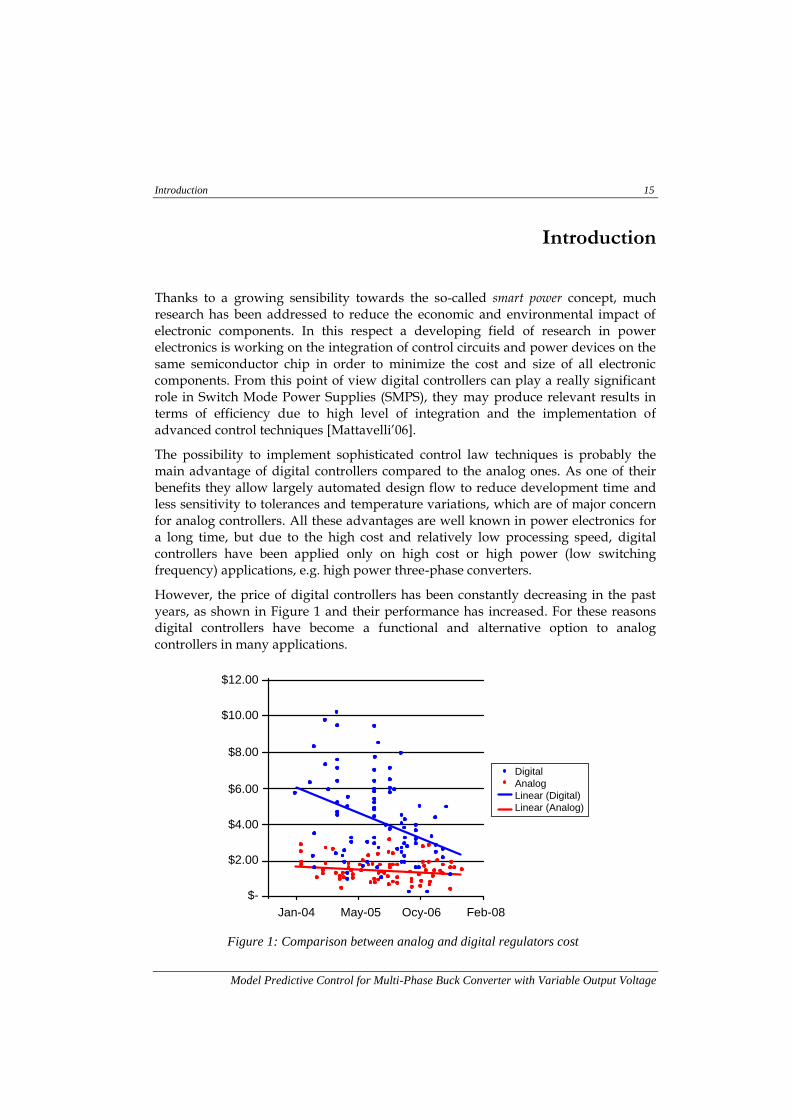
However, the price of digital controllers has been constantly decreasing in the past years, as shown in Figure 1 and their performance has increased. For these reasons digital controllers have become a functional and alternative option to analog controllers in many applications.
Digital
Analog
Linear (Digital)
Linear (Analog)
$12.00
$10.00
$8.00
$6.00
$-
$4.00
$2.00
Jan-04 May-05 Ocy-06 Feb-08
Figure 1: Comparison between analog and digital regulators cost
16 Introduction
Model Predictive Control for Multi-Phase Buck Converter with Variable Output Voltage
Among the different digital control techniques this work focuses on discrete-time Model Predictive Control (MPC) and on the possibility to exploit predicted information of the reference. In some applications advanced knowledge of voltage references area available and may be used in order to improve reference tracking. An example is given by the Envelope Elimination and Restoration (EER) technique and the Envelope Tracking (ET) technique, used in Radio Frequency (RF)transmitters to cut down the losses in the amplifier [Vasic'10].
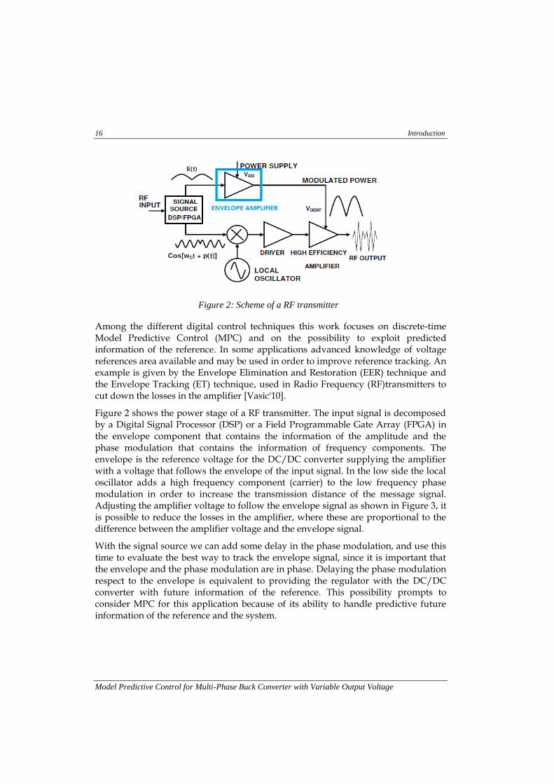
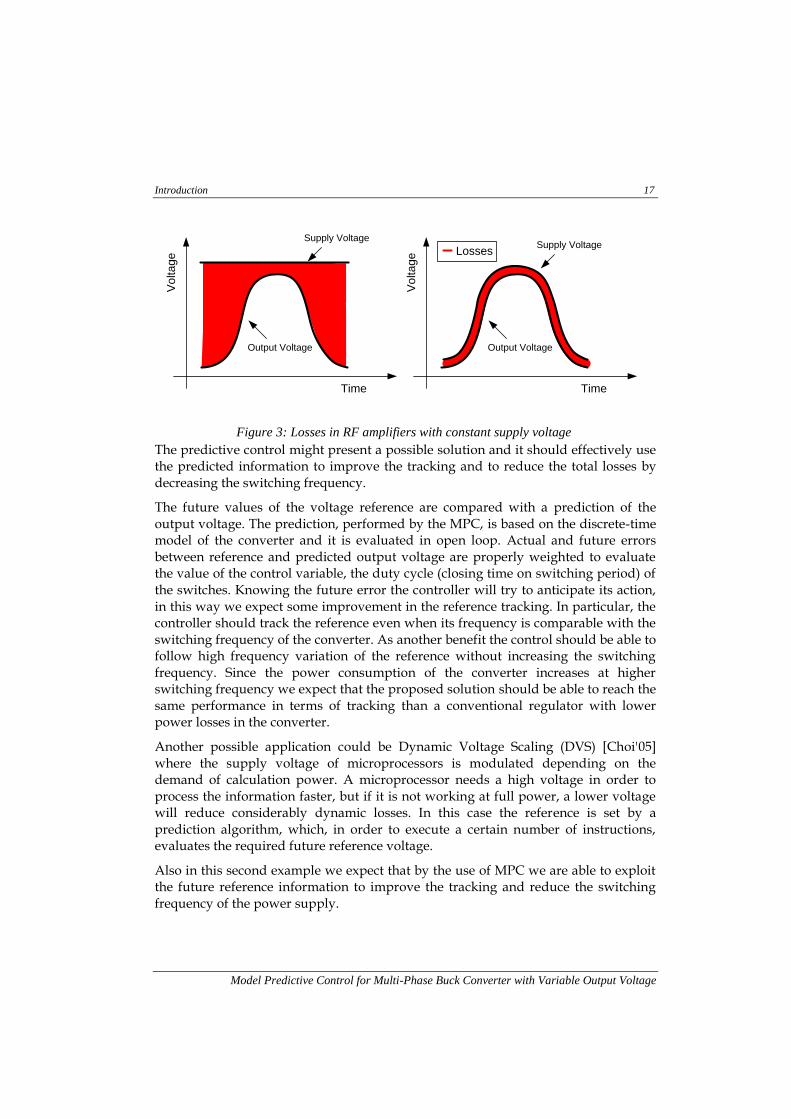
Figure 2 shows the power stage of a RF transmitter. The input signal is decomposed by a Digital Signal Processor (DSP) or a Field Programmable Gate Array (FPGA) in the envelope component that contains the information of the amplitude and the phase modulation that contains the information of frequency components. The envelope is the reference voltage for the DC/DC converter supplying the amplifier with a voltage that follows the envelope of the input signal. In the low side the local oscillator adds a high frequency component (carrier) to the low frequency phase modulation in order to increase the transmission distance of the message signal. Adjusting the amplifier voltage to follow the envelope signal as shown in Figure 3, it is possible to reduce the losses in the amplifier, where these are proportional to the difference between the amplifier voltage and the envelope signal.
With the signal source we can add some delay in the phase modulation, and use this time to evaluate the best way to track the envelope signal, since it is important that the envelope and the phase modulation are in phase. Delaying the phase modulation respect to the envelope is equivalent to providing the regulator with the DC/DC converter with future information of the reference. This possibility prompts to consider MPC for this application because of its ability to handle predictive future information of the reference and the system.
Figure 2: Scheme of a RF transmitter
Introduction 17
Model Predictive Control for Multi-Phase Buck Converter with Variable Output Voltage
The predictive control might present a possible solution and it should effectively use the predicted information to improve the tracking and to reduce the total losses by decreasing the switching frequency.
The future values of the voltage reference are compared with a prediction of the output voltage. The prediction, performed by the MPC, is based on the discrete-time model of the converter and it is evaluated in open loop. Actual and future errors between reference and predicted output voltage are properly weighted to evaluate the value of the control variable, the duty cycle (closing time on switching period) of the switches. Knowing the future error the controller will try to anticipate its action, in this way we expect some improvement in the reference tracking. In particular, the controller should track the reference even when its frequency is comparable with the switching frequency of the converter. As another benefit the control should be able to follow high frequency variation of the reference without increasing the switching frequency. Since the power consumption of the converter increases at higher switching frequency we expect that the proposed solution should be able to reach the same performance in terms of tracking than a conventional regulator with lower power losses in the converter.
Another possible application could be Dynamic Voltage Scaling (DVS) [Choi'05] where the supply voltage of microprocessors is modulated depending on the demand of calculation power. A microprocessor needs a high voltage in order to process the information faster, but if it is not working at full power, a lower voltage will reduce considerably dynamic losses. In this case the reference is set by a prediction algorithm, which, in order to execute a certain number of instructions, evaluates the required future reference voltage.
Also in this second example we expect that by the use of MPC we are able to exploit the future reference information to improve the tracking and reduce the switching frequency of the power supply.
Time
Vo
lta
ge
Supply Voltage
Output Voltage
Losses
Time
Vo
lta
ge
Supply Voltage
Output Voltage
Figure 3: Losses in RF amplifiers with constant supply voltage
18 Introduction
Model Predictive Control for Multi-Phase Buck Converter with Variable Output Voltage
After this introduction which explained briefly the motivation and the objective of this work, the next two chapters provide some background.
Depending on its purpose, a model can be more or less complex and reproduce with higher or lower precision the behavior of the system. So, for simulation purpose the model has high level of detail in order to have an accurate representation of the plant (the system under control), while for control design the model is simpler, but still able to reproduce the dominant behavior of system. The first chapter will look into the different models used in simulation to design the control and to validate it. The systematic way to obtain a time invariant linear model of a SMPS is shown and subsequently the discretization method is presented. Due to limitation of the averaged model a better model called Multi-Frequency small-signal model is used during the design stage.
The second chapter introduces some basic knowledge of MPC: cost function, open loop prediction and receding horizon. Finally the used method to integrate an integral action is presented and its two possible formulations are discussed. There are different approaches to MPC, but they all have some common features, as the definition of a cost function the open loop prediction and the receding horizon. This chapter will introduce the MPC starting from some basic knowledge, and eventually two methods to add integral action and the associated anti wind-up schemes. Two proposed approaches are outlined, highlighting their differences and advantages. The problematic of its feasibility will be discussed and the delay compensator is used to stabilize the overall control system.
The third chapter will describe the design method based on Genetic Algorithms (GA). Firstly some basic concepts about GA are briefly introduced. Then we will see how GA has been implemented in the design of the MPC. The final control architecture implemented on an FPGA is described underling some implementation issues. In particular a new Digital Multiphase Modulator is used, particularly indicated for digital controllers.
In the fourth chapter the simulation results of the design process performed with Matlab and Matlab/Simulink are shown. Validation results with the simulator Simplorer are presented, in which the overall controller is described with the same VHDL code as used for the FPGA implementation. Simulation results comparing this solution with a conventional regulator are also included.
Finally conclusions of this work are presented as well as possible future developments and improvements.
Modeling a MP Buck Converter 19
Model Predictive Control for Multi-Phase Buck Converter with Variable Output Voltage
Chapter: 1 Modeling a MP Buck Converter
The purpose of this chapter is to present the models used to describe the behavior of the four-phase Buck converter used for the simulation and experimental results. First, the features of the converter and the model used for simulation are presented, later, the averaged model is reviewed to obtain two different models used for different purposes: a discrete-time averaged model used by the MPC and the Kalman filter to estimate the future values of the output voltage; a more accurate Multi-Frequency model used in simulation during the control design process.
I. Choice of the converter
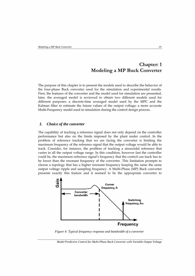
The capability of tracking a reference signal does not only depend on the controller performance but also on the limits imposed by the plant under control. In the problem of reference tracking that we are facing the converter is limiting the maximum frequency of the reference signal that the output voltage would be able to track. Consider, for instance, the problem of tracking a sinusoidal reference that varies in all the output voltage range. In this condition, however fast the controller could be, the maximum reference signal’s frequency that the control can track has to be lower than the resonant frequency of the converter. This limitation prompts to choose a topology that has a higher resonant frequency keeping the same the same output voltage ripple and sampling frequency. A Multi-Phase (MP) Buck converter presents exactly this feature and it seemed to be the appropriate converter to
Figure 4: Typical frequency response and bandwidth of a converter
20 Modeling a MP Buck Converter
Model Predictive Control for Multi-Phase Buck Converter with Variable Output Voltage
maximize the trackable reference bandwidth.
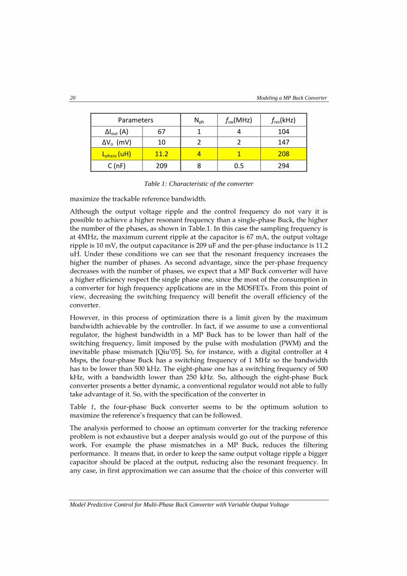
Although the output voltage ripple and the control frequency do not vary it is possible to achieve a higher resonant frequency than a single-phase Buck, the higher the number of the phases, as shown in Table.1. In this case the sampling frequency is at 4MHz, the maximum current ripple at the capacitor is 67 mA, the output voltage ripple is 10 mV, the output capacitance is 209 uF and the per-phase inductance is 11.2 uH. Under these conditions we can see that the resonant frequency increases the higher the number of phases. As second advantage, since the per-phase frequency decreases with the number of phases, we expect that a MP Buck converter will have a higher efficiency respect the single phase one, since the most of the consumption in a converter for high frequency applications are in the MOSFETs. From this point of view, decreasing the switching frequency will benefit the overall efficiency of the converter.
However, in this process of optimization there is a limit given by the maximum bandwidth achievable by the controller. In fact, if we assume to use a conventional regulator, the highest bandwidth in a MP Buck has to be lower than half of the switching frequency, limit imposed by the pulse with modulation (PWM) and the inevitable phase mismatch [Qiu’05]. So, for instance, with a digital controller at 4 Msps, the four-phase Buck has a switching frequency of 1 MHz so the bandwidth has to be lower than 500 kHz. The eight-phase one has a switching frequency of 500 kHz, with a bandwidth lower than 250 kHz. So, although the eight-phase Buck converter presents a better dynamic, a conventional regulator would not able to fully take advantage of it. So, with the specification of the converter in
Table 1, the four-phase Buck converter seems to be the optimum solution to maximize the reference’s frequency that can be followed.
The analysis performed to choose an optimum converter for the tracking reference problem is not exhaustive but a deeper analysis would go out of the purpose of this work. For example the phase mismatches in a MP Buck, reduces the filtering performance. It means that, in order to keep the same output voltage ripple a bigger capacitor should be placed at the output, reducing also the resonant frequency. In any case, in first approximation we can assume that the choice of this converter will
Parameters Nph fsw(MHz) fres(kHz)
∆Iout (A) 67 1 4 104
∆Vo (mV) 10 2 2 147
Lphase (uH) 11.2 4 1 208
C (nF) 209 8 0.5 294
Table 1: Characteristic of the converter
Modeling a MP Buck Converter 21
Model Predictive Control for Multi-Phase Buck Converter with Variable Output Voltage
give the possibility to follow a higher bandwidth reference signal than a single-phase Buck.
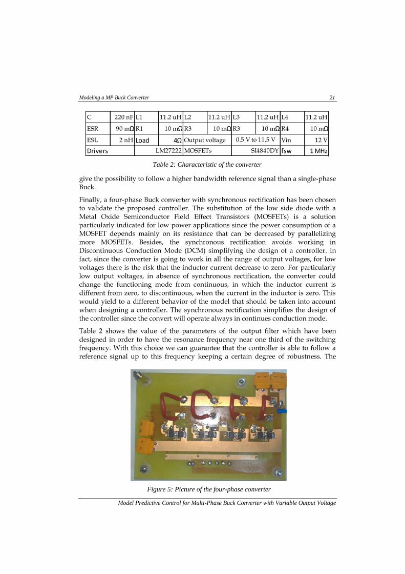
Finally, a four-phase Buck converter with synchronous rectification has been chosen to validate the proposed controller. The substitution of the low side diode with a Metal Oxide Semiconductor Field Effect Transistors (MOSFETs) is a solution particularly indicated for low power applications since the power consumption of a MOSFET depends mainly on its resistance that can be decreased by parallelizing more MOSFETs. Besides, the synchronous rectification avoids working in Discontinuous Conduction Mode (DCM) simplifying the design of a controller. In fact, since the converter is going to work in all the range of output voltages, for low voltages there is the risk that the inductor current decrease to zero. For particularly low output voltages, in absence of synchronous rectification, the converter could change the functioning mode from continuous, in which the inductor current is different from zero, to discontinuous, when the current in the inductor is zero. This would yield to a different behavior of the model that should be taken into account when designing a controller. The synchronous rectification simplifies the design of the controller since the convert will operate always in continues conduction mode.
Table 2 shows the value of the parameters of the output filter which have been designed in order to have the resonance frequency near one third of the switching frequency. With this choice we can guarantee that the controller is able to follow a reference signal up to this frequency keeping a certain degree of robustness. The
Figure 5: Picture of the four-phase converter
Table 2: Characteristic of the converter
C 220 nF L1 11.2 uH L2 11.2 uH L3 11.2 uH L4 11.2 uH
ESR 90 mΩ R1 10 mΩ R3 10 mΩ R3 10 mΩ R4 10 mΩ
ESL 2 nH Load 4Ω Output voltage Vin 12 V
fsw 1 MHzLM27222Drivers
0.5 V to 11.5 V
MOSFETs SI4840DY
22 Modeling a MP Buck Converter
Model Predictive Control for Multi-Phase Buck Converter with Variable Output Voltage
MOSFETs have been chosen for having low consumption at this switching frequency, while the drivers are indicated for high frequency application since the delay between driving signal and gate voltage of the MOSFET is particularly low, around 10ns.
I. The Switched model
This model is used to validate the controller’s performance in simulation before implementing it on a prototype. For this reason the model has to take into account all those parasitic elements that can affect the control performance and that are usually neglected in the control-oriented model.
In order to validate the control stage Simplorer has been chosen among several electronic-circuit simulators due to the possibility to use VHDL-AMS code to model the digital controller. Since the digital controller is implemented on a FPGA, a VHDL description of the control behaviour is used to program it. In Simplorer the same code has been used to model the controller that ensures a good model of the control behaviour in simulation. The control architecture is described with details in the
Vin
L1
C
Load
L2
L3
i1
i2
i3
c1
c2
c3
Vout
i4c4
L4
ESR
ESL
R1
R2
R3
R4
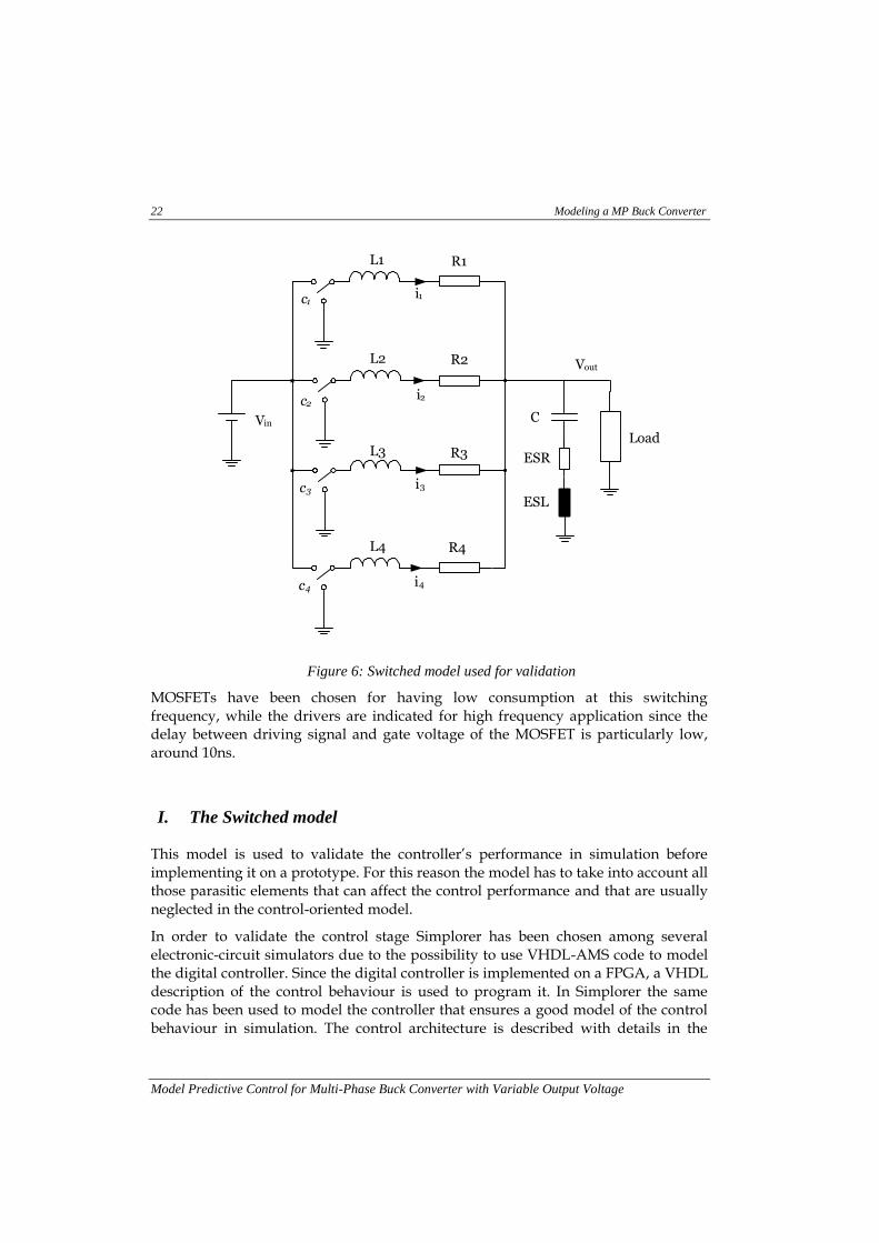
Figure 6: Switched model used for validation
Modeling a MP Buck Converter 23
Model Predictive Control for Multi-Phase Buck Converter with Variable Output Voltage
third chapter, here we underline the only difference between the simulation model in Simplorer and the code used to program the FPGA that is the introduction in the simulation model of a delay in the driving signal of the MOSFETs of two clock period that represents the internal delays of the drivers.
Figure 6 shows the model of the converter used to model the controller. Being a switched model it can represent correctly the high frequency effects caused by the pulse width modulation (PWM) that are particularly determining especially for a MP converter, because together with the phase mismatch the PWM limits the control bandwidth to be lower than half of the switching frequency [Qiu’05]. The series inductor resistances are important to be considered since they change the input-output voltage ratio, on which the control law relays. The equivalent series resistance (ESR) and the equivalent series inductance (ESL) of the capacitor influence both output voltage ripple and the dynamic of the system, so they have to be taken into account too.
Another important parasitic element to consider is time delay of the driver. Although drivers have been chosen for having a small input-output delay, it can still affect the stability of the overall system. These delays have been modelled within the digital controller as a delay of few clock periods on the driven signals of the MOSFETs.
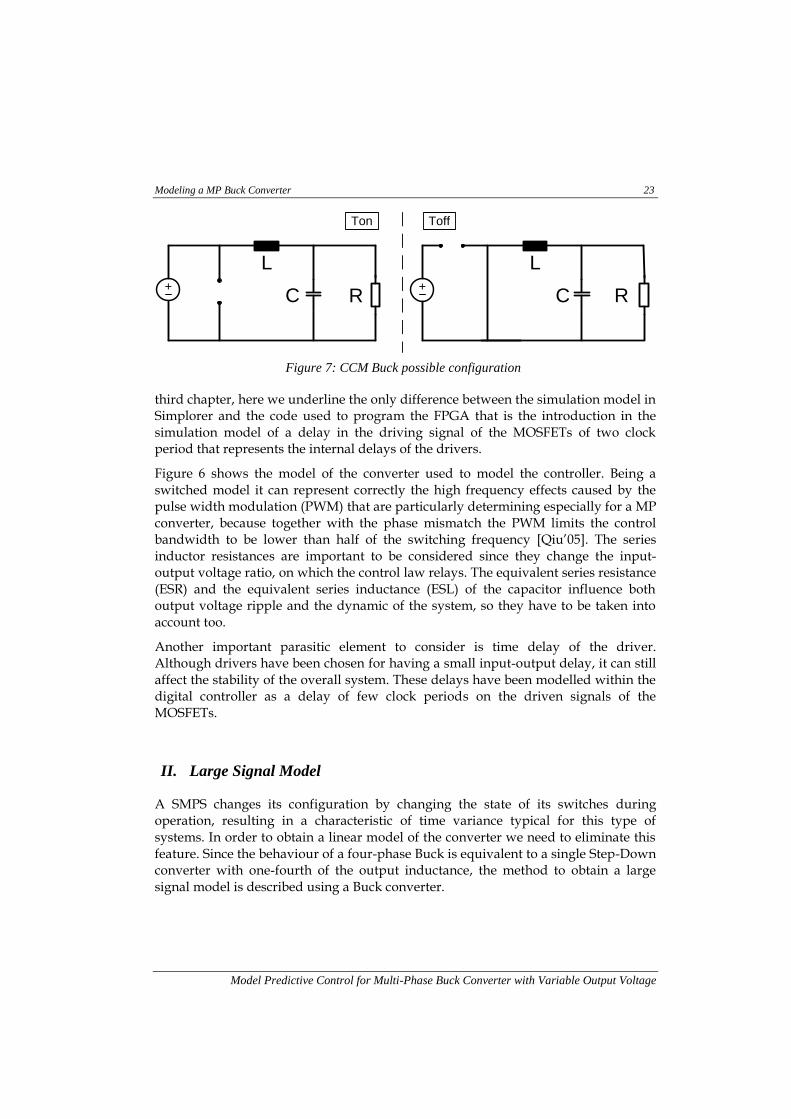
II. Large Signal Model
A SMPS changes its configuration by changing the state of its switches during operation, resulting in a characteristic of time variance typical for this type of systems. In order to obtain a linear model of the converter we need to eliminate this feature. Since the behaviour of a four-phase Buck is equivalent to a single Step-Down converter with one-fourth of the output inductance, the method to obtain a large signal model is described using a Buck converter.
L
C R+
L
C+
R
Ton Toff
Figure 7: CCM Buck possible configuration
24 Modeling a MP Buck Converter
Model Predictive Control for Multi-Phase Buck Converter with Variable Output Voltage
In this case, the switches determine two different configurations during a switching period, as it is possible to see in Figure 8. The on-off state is referred to the high-side switch, while the low-side one is complementary. This behaviour determines the presence of small ripples on the output current and output voltage waveform. We can obtain a simpler model that reproduces the dominant behaviour of the system by eliminating the ripples. This is equivalent to average over one switching period the signals of the converter, obtaining the averaged model of the converter that is able to reproduce the large signal behaviour.
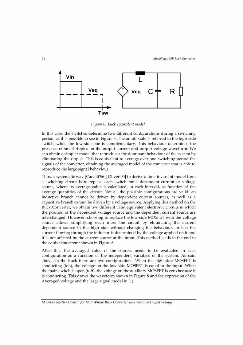
Thus, a systematic way [Canalli’96][ Oliver’00] to derive a time-invariant model from a switching circuit is to replace each switch for a dependent current or voltage source, where its average value is calculated, in each interval, as function of the average quantities of the circuit. Not all the possible configurations are valid: an inductive branch cannot be driven by dependent current sources, as well as a capacitive branch cannot be driven by a voltage source. Applying this method on the Buck Converter, we obtain two different valid equivalent electronic circuits in which the position of the dependent voltage source and the dependent current source are interchanged. However, choosing to replace the low-side MOSFET with the voltage source allows simplifying even more the circuit by eliminating the current dependent source in the high side without changing the behaviour. In fact the current flowing through the inductor is determined by the voltage applied on it and it is not affected by the current source at the input. This method leads in the end to the equivalent circuit shown in Figure 8.
After this, the averaged value of the sources needs to be evaluated in each configuration as a function of the independent variables of the system. As said above, in the Buck there are two configurations. When the high side MOSFET is conducting (ton), the voltage on the low-side MOSFET is equal to the input. When the main switch is open (toff), the voltage on the auxiliary MOSFET is zero because it is conducting. This draws the waveform shown in Figure 8 and the expression of the Averaged voltage and the large signal model in (1).
L
C R+
-
Vin
Veq Veq
Tsw
Figure 8: Buck equivalent model
Modeling a MP Buck Converter 25
Model Predictive Control for Multi-Phase Buck Converter with Variable Output Voltage
( ) ( ) ( )
Once all the dependent sources are defined, writing the system of differential equation that
describes the behavior of the converter is straight forward. The system in (2) describes the
averaged behavior of the MP Buck converter. Since, the voltage on the MOSFET depends on the input voltage (Vin) and on the duty cycle (d), if the input voltage varies in the time the (2) is a non-linear system, therefore, the next step in the modelling of the converter is to linearize the large signal model around the operation point, in order to arrive to a control-oriented description.
( )
( ( )
( )
)
( )
( ( ) ( ))
( )
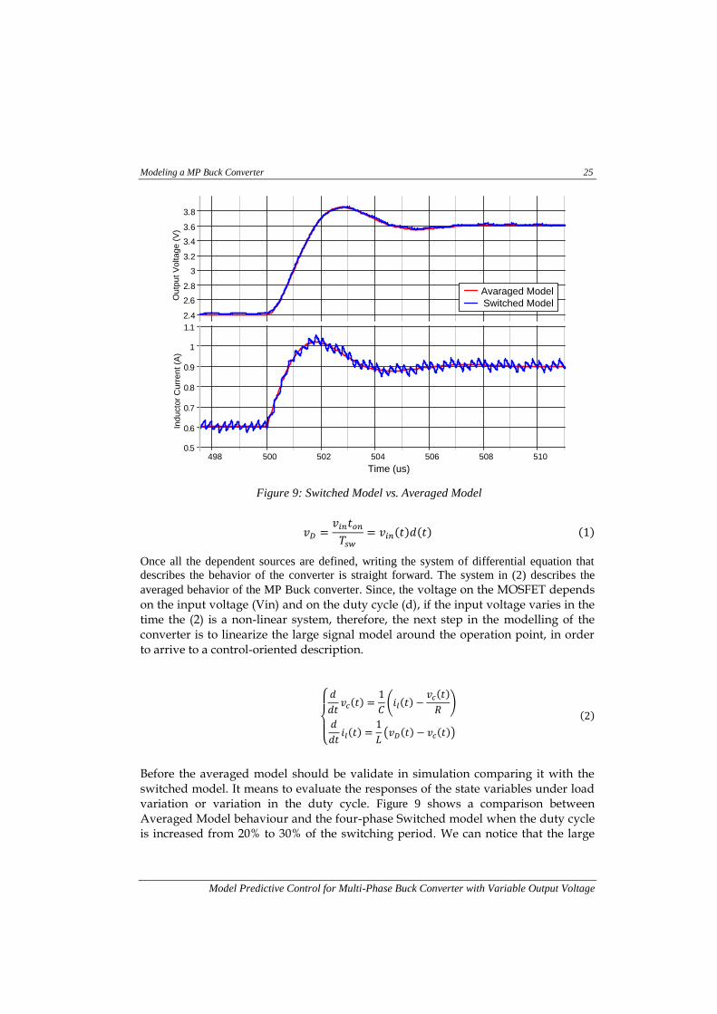
Before the averaged model should be validate in simulation comparing it with the switched model. It means to evaluate the responses of the state variables under load variation or variation in the duty cycle. Figure 9 shows a comparison between Averaged Model behaviour and the four-phase Switched model when the duty cycle is increased from 20% to 30% of the switching period. We can notice that the large
Ou
tpu
t V
olta
ge
(V
)
2.4
2.6
2.8
3
3.2
3.4
3.6
3.8
498 500 502 504 506 508 510
Ind
ucto
r C
urr
en
t (A
)
0.5
0.6
0.7
0.8
0.9
1
1.1
Time (us)
Avaraged Model
Switched Model
Figure 9: Switched Model vs. Averaged Model
26 Modeling a MP Buck Converter
Model Predictive Control for Multi-Phase Buck Converter with Variable Output Voltage
signal model depreciates the voltage and current ripple due to the switching frequency, but shows the same large dynamic. Once we have validated all the system state variables we are sure that all other variables of the system are well described.
III. Discrete time model
If, at first approximation, we consider the voltage supply constant, the resulting system is not only time-invariant but also linear. In this case the system of equation in (2) can be rewritten in matrix form as in (3), where the matrices are defined an in (4).
( ) ( ) ( )
( ) ( ) ( )
[
] [
]
[ ]
( )
Once obtained the linearized model, it is possible to evaluate the discrete-time model. There are different methods to obtain a discretized model, each one with its advantages and drawbacks. Most of them are based on substituting the variable s of the corresponding transfer function with a proper function in the transformer z. All of them are good approximation of continues time model. However, there is another method that describes correctly the evolution of the system without approximation. This consists of applying matrix exponential and zero order hold to the state space system in continues time [Bolzern’09], yielding to the equivalent system of difference equations (5).
( ) ( ) ( )
( ) ( ) ( )
The value of the matrices obtained by applying the discretization to the state-space
continuous system is shown in (6), where Ts is the sampling time.
Modeling a MP Buck Converter 27
Model Predictive Control for Multi-Phase Buck Converter with Variable Output Voltage
∫
( )
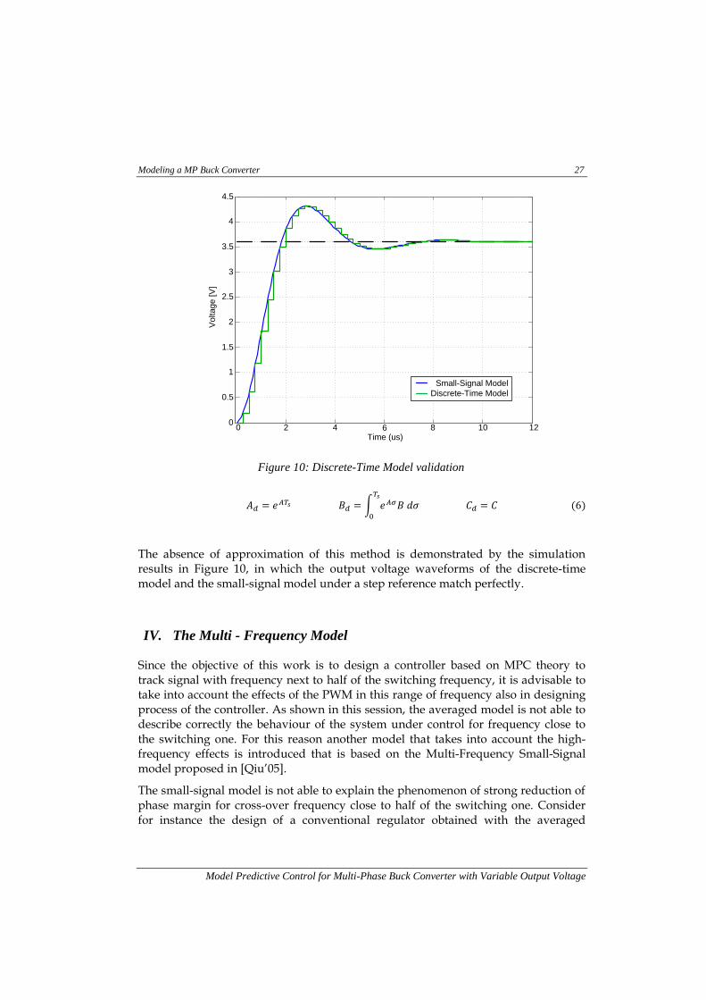
The absence of approximation of this method is demonstrated by the simulation results in Figure 10, in which the output voltage waveforms of the discrete-time model and the small-signal model under a step reference match perfectly.
IV. The Multi - Frequency Model
Since the objective of this work is to design a controller based on MPC theory to track signal with frequency next to half of the switching frequency, it is advisable to take into account the effects of the PWM in this range of frequency also in designing process of the controller. As shown in this session, the averaged model is not able to describe correctly the behaviour of the system under control for frequency close to the switching one. For this reason another model that takes into account the high-frequency effects is introduced that is based on the Multi-Frequency Small-Signal model proposed in [Qiu’05].
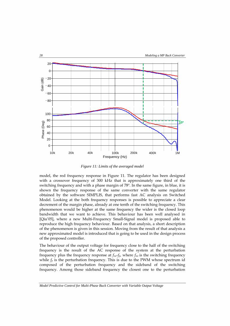
The small-signal model is not able to explain the phenomenon of strong reduction of phase margin for cross-over frequency close to half of the switching one. Consider for instance the design of a conventional regulator obtained with the averaged
0 2 4 6 8 10 120
0.5
1
1.5
2
2.5
3
3.5
4
4.5
Time (us)
Vo
lta
ge
[V
]
Small-Signal Model
Discrete-Time Model
Figure 10: Discrete-Time Model validation
28 Modeling a MP Buck Converter
Model Predictive Control for Multi-Phase Buck Converter with Variable Output Voltage
model, the red frequency response in Figure 11. The regulator has been designed with a crossover frequency of 300 kHz that is approximately one third of the switching frequency and with a phase margin of 78º. In the same figure, in blue, it is shown the frequency response of the same converter with the same regulator obtained by the software SIMPLIS, that performs fast AC analysis on Switched Model. Looking at the both frequency responses is possible to appreciate a clear decrement of the margin phase, already at one tenth of the switching frequency. This phenomenon would be higher at the same frequency the wider is the closed loop bandwidth that we want to achieve. This behaviour has been well analysed in [Qiu’05], where a new Multi-Frequency Small-Signal model is proposed able to reproduce the high frequency behaviour. Based on that analysis, a short description of the phenomenon is given in this session. Moving from the result of that analysis a new approximated model is introduced that is going to be used in the design process of the proposed controller.
The behaviour of the output voltage for frequency close to the half of the switching frequency is the result of the AC response of the system at the perturbation frequency plus the frequency response at fsw-fp, where fsw is the switching frequency while fp is the perturbation frequency. This is due to the PWM whose spectrum id composed of the perturbation frequency and the sideband of the switching frequency. Among those sideband frequency the closest one to the perturbation
Ga
in (
dB
)
- 80
- 60
- 40
- 20
0
20
10k 20k 40k 100k 200k 400k 1M
Ph
ase
(D
eg)
0
20
40
60
80
100
10º
Frequency (Hz)
Figure 11: Limits of the averaged model
Modeling a MP Buck Converter 29
Model Predictive Control for Multi-Phase Buck Converter with Variable Output Voltage
frequency is indeed the component at fsw-fp. If the bandwidth of the controller is small, this component is well-filtered thus it does not affect the frequency response. Instead, for control bandwidth close to half of the switching frequency this attenuation diminishes, so that this component interferes with the frequency response of the system. Thus, the modified Multi-Frequency loop obtained loop gain is obtained as in (7), where ( ) is the small-signal loop gain evaluated at perturbation angular frequency, while ( ) is the small-signal loop gain evaluated at the perturbation frequency minus the switching angular frequency.
( )
( ) ( )
This analysis has been extended to a MP Buck converter, where, in case of perfect match between the phases, this phenomenon does not happen at the switching frequency but at N times the switching frequency, with N the number of phases. The previous expression adapted to a two-phase Buck as in (9).
( )
( )
( )
It is clear that in case the two phase inductances were identical there would not be this effect at the switching frequency. Since a perfect match among the phase is impossible, the maximum bandwidth of conventional regulator in case of a MP converter is still limited by the switching frequency.
Now the idea is to adapt the expression in () to the design method for the proposed controller explained in the next chapter. Since the design of the controller is performed by using Matlab/Simulink, this expression is not really useful in this form because Simulink cannot perform frequency analysis at different frequency at the same time. The second problem is that the decrement of the phase margin depends on the position of the cross-over frequency; it means that the high frequency effect should be evaluated for every different design. This way is not convenient for the method used for the design of the controller. For this reason it has been decided to approximate the expression in () with a notch filter.
A notch filter has been added to the transfer function of the Buck converter in order to represent the decrease of phase margin around the switching frequency. Its parameters have been chosen in order to have a frequency response similar in phase

30 Modeling a MP Buck Converter
Model Predictive Control for Multi-Phase Buck Converter with Variable Output Voltage
and gain to the expression in (9), where the loop gain has been chosen in order to have a cross-over frequency of one third of the switching one.
( ) ( )
In this way it has been possible to evaluate the high-frequency effects once for all the possible control design, where it is assumed that none of them can overcome the bandwidth defined to evaluate the expression in (9).
Proposed Control Approach 31
Model Predictive Control for Multi-Phase Buck Converter with Variable Output Voltage
Chapter: 2 Proposed Control Approach
As seen in the Introduction, there are several applications of power electronics in which the output voltage reference, its desired future values, are known in advance. So, the idea of this work is to use this information in order design a regulator able to improve the tracking performance of conventional regulators. Model Predictive Control seemed to be an appropriate control technique to accomplish this objective.
In this chapter the Model Predictive Control is introduced, underling those characteristic there are useful for the purpose of this work. Afterwards, two different approaches of this method and a design method are suggested.
do not use this information to track the The idea of this work is to use t that the out Usually the future values of the reference are considered to be equal to its current value, due to the fact that in general these value are not supposed to be known, but for the particular applications discussed in the introduction, this can be the case.
I. Introduction to Model Predictive Control
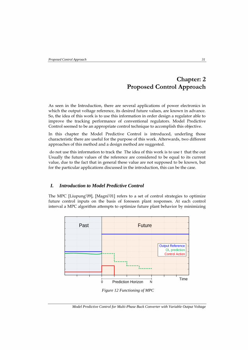
The MPC [Liupung’09], [Magni’01] refers to a set of control strategies to optimize future control inputs on the basis of foreseen plant responses. At each control interval a MPC algorithm attempts to optimize future plant behavior by minimizing
Past Future
Time Prediction Horizon
Output Reference
OL prediction
Control Action
N0
Figure 12 Functioning of MPC
32 Proposed Control Approach
Model Predictive Control for Multi-Phase Buck Converter with Variable Output Voltage
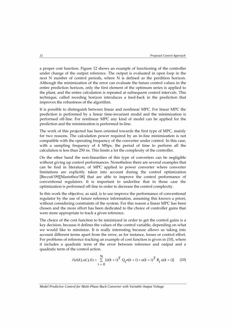
a proper cost function. Figure 12 shows an example of functioning of the controller under change of the output reference. The output is evaluated in open loop in the next N number of control periods, where N is defined as the perdition horizon. Although the minimization of the error can evaluate the future control values in the entire prediction horizon, only the first element of the optimum series is applied to the plant, and the entire calculation is repeated at subsequent control intervals. This technique, called receding horizon introduces a feed-back in the prediction that improves the robustness of the algorithm.
It is possible to distinguish between linear and nonlinear MPC. For linear MPC the prediction is performed by a linear time-invariant model and the minimization is performed off-line. For nonlinear MPC any kind of model can be applied for the prediction and the minimization is performed in-line.
The work of this projected has been oriented towards the first type of MPC, mainly for two reasons. The calculation power required by an in-line minimization is not compatible with the operating frequency of the converter under control. In this case, with a sampling frequency of 4 MSps, the period of time to perform all the calculation is less than 250 ns. This limits a lot the complexity of the controller.
On the other hand the non-linearities of this type of converters can be negligible without giving up control performances. Nonetheless there are several examples that can be find in literature, of MPC applied to power converter where converter limitations are explicitly taken into account during the control optimization [Beccuti’09][Mariethoz’08] that are able to improve the control performance of conventional regulators. It is important to underline that in those case the optimization is performed off-line in order to decrease the control complexity.
In this work the objective, as said, is to use improve the performance of conventional regulator by the use of future reference information, assuming this known a priori, without considering constraints of the system. For this reason a linear MPC has been chosen and the more effort has been dedicated to the choice of controller gains that were more appropriate to track a given reference.
The choice of the cost function to be minimized in order to get the control gains is a key decision, because it defines the values of the control variable, depending on what we would like to minimize. It is really interesting because allows us taking into account different terms apart from the error, as for instance, losses or control effort. For problems of reference tracking an example of cost function is given in (10), where it includes a quadratic term of the error between reference and output and a quadratic term of the control action.
N
0i
)]( i
)()(i
Q )([)),(),(( ikuRTikuikeTikekukeJ (10)
Proposed Control Approach 33
Model Predictive Control for Multi-Phase Buck Converter with Variable Output Voltage
)()()( ikyikyike
The minimization of this function finds the optimum value for the input variables that reduce the error, keeping limited the control input. It is important to underline that the optimum solution will depend on the weight coefficient Q and R, and on the prediction horizon N; these parameters are a degree of freedom. The control will tend to be faster if the value of Q is higher than R, but this will cause higher stress on the control variable with the risk of entering often in saturation. Finally the right value to assign to these two parameters will be a designer decision, based on the behavior of inputs and outputs during the simulation of the closed loop.
The second common feature of all the versions of the predictive control is the evaluation of the future response of the plant through a discrete time-model of the system. The model can be whatever depending on the purpose and the approach of the designer; in this case the discrete-time model has been introduced in the previous chapter. So, the idea is that the future output is completely determined by the future values of the control input and the open loop response, where the latter is the autonomous behavior of the plant in absence of the control action. So, using the last measured value of the state vector it is possible to evaluate the future response as in (11), where x(k) is the current value of the state vector, U(k) is the vector of the future inputs and Ac and Bc are matrices derived from the discrete-time model matrices as in (12).
)()()1( kUc
Bkxc
AkY (11)
)1(
)(
1
00
)(
)(
)1(
Nku
ku
CBBnCA
CB
kxnCA
CA
Nky
ky
(12)
By comparing the future reference value and the open loop prediction it is possible to obtain determine the future control values that minimize the error between them. Ignoring the model constraints, the minimization of the cost function in (10) using the open loop prediction in (11) leads to a linear control law in (13) where Kmpc represent the feedback gains of the predictive controller.
)()1()( kxAkYKkU cmpc
(13)
34 Proposed Control Approach
Model Predictive Control for Multi-Phase Buck Converter with Variable Output Voltage
cQ
cB
cR
cB
cQ
cB
mpcK '1)'(
(14)
II. Integral action
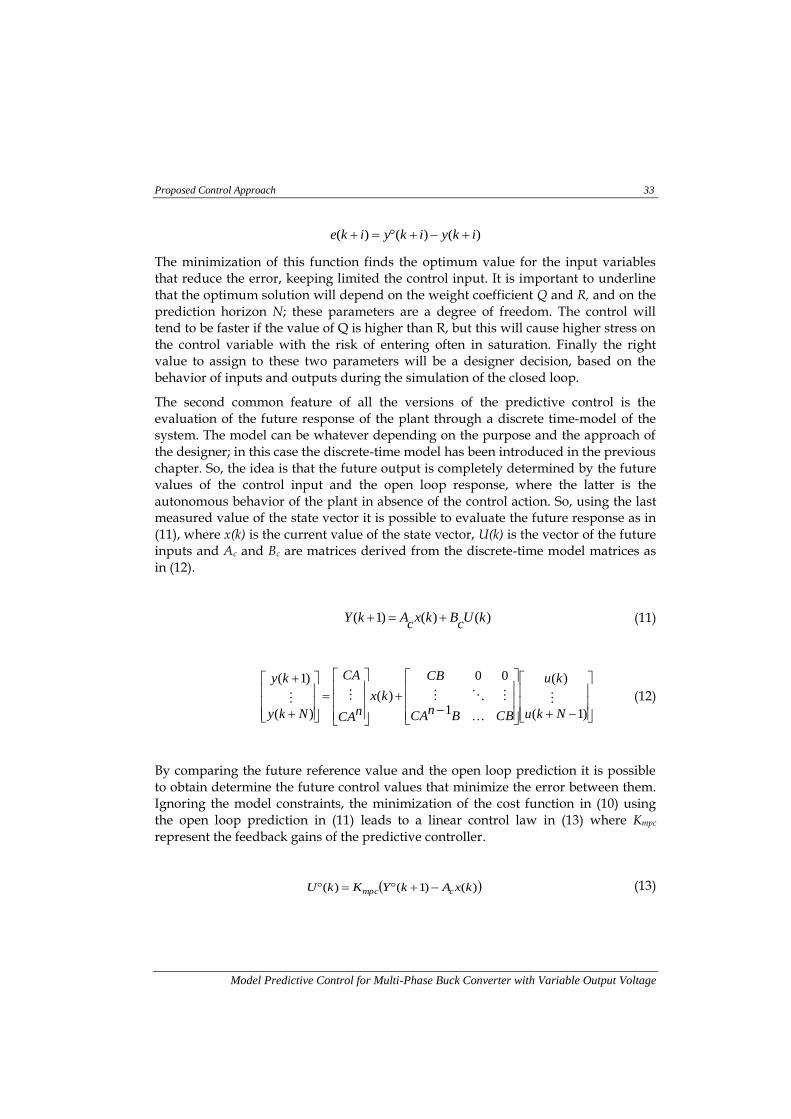
With the definition of the control law as in (14) or (17) it is not possible to guarantee a steady-state error to zero under variation of the system from the nominal values or load variation. There are at least two solutions at this problem: adding an integral action of the error in the cost function, as in [Mariethoz’08]; or explicitly adding an integral action in the regulator, considering it as part of the plant under control. For simplicity of the solution the second method has been applied in this work.
In the z-transform there are two different way to perform integration: using a strictly proper integrator or a non-strictly proper one. Both have some advantages and disadvantages, as examined below, in order to be able to choose which one is more appropriate for the purpose of this work.
The most important advantage of the strictly proper integrator is its feasibility; the control variable depends only on the previous value of the integral action (d) and of the input (uMPC) (15). It means we have an entire switching period in order to evaluate the next value of the integral action.
)()()1( kukuku MPC ( )
On the other hand there are some pitfalls. As said, this technique of inserting the integral action in the MPC control law yields to consider the integrator as part of the system. Therefore the integral control law has to be added in the equations of the system, obtaining its new expression as in (16 and 17).
)( )( )1(
)()()1(
kukuku
kBukAxkx
MPC
( )
MPC1
z-1Plant
err umpc u y
Figure 13: Strictly-proper integral action
Proposed Control Approach 35
Model Predictive Control for Multi-Phase Buck Converter with Variable Output Voltage
)(0
)(
)(
0)1(
)1(ku
Iku
kx
I
BA
ku
kxMPC
( )
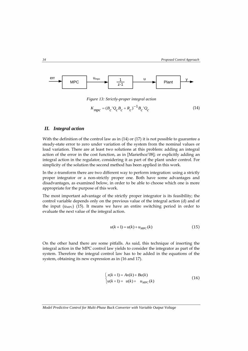
Reminding that the prediction is performed in open loop, it is possible to see that the expression of the integral action adds some more uncertainty in the prediction. The value of the control variable is supposed to be known at each time, because it is assigned by the regulator, but clearly the real value of the input that acts on the plant might be different, due to possible disturbance. This method is not robust against disturbances on the control variable. On the contrary, the proper formulation of the integral action (18) does not produce this effect but it has the important disadvantage of not being feasible.
)()1()( kukuku MPC ( )
The current value of the integral action depends on its previous value and on the current value of the input. It means that the controller should be able to evaluate the control input value in zero time not to produce a delay in the control action that can affect the stability of the system. On other hand the integrator yields to an interesting formulation of the plant model for two reasons: it simplifies the anti-wind up technique and, more importantly, it simplifies the definition of the state reference, as it will be explained in the next session.
In order to consider the proper integrator as part of the system for this, it is useful to rewrite the expression of the model introducing a new definition of the state variables, called delta transform [Middleton’90], as in (18).
)()1()1( kxkxkx iii )1()()( kukukuMPC ( )
Starting from the state space model, after some modifications (19) it is possible to rewrite the system in the new variables as in (20), whose matrix form is shown in (21).
MPCz
z-1Plant
err umpc u y
Figure 14: Non-strictly proper integral action
36 Proposed Control Approach
Model Predictive Control for Multi-Phase Buck Converter with Variable Output Voltage
)1()1()()(
)()()()()1(
kykykCxky
kxkxkBukAxkx
)1()1()()(
)1()1()()()()1(
kykCxkCxky
kBukAxkxkBukAxkx ( )
))()1(()()1(
))1()(())1()(()()1(
kxkxCkyky
kukuBkxkxAkxkx
(21) )( )( )( )1(
)( )( )1(
kuCBkxCAkyky
kuBkxAkx
MPC
MPC
)(
)( 10 )(
)()(
)(0
)1(
)1(
ky
kxky
kuCB
B
ky
kx
ICA
A
ky
kxMPC
(22)
The new system presents a new state-variable that reflects the introduction of the integral action, with the difference that the new variable is not the integral signal, but the same output. It means the prediction of the state is now performed by the knowledge of the state vector and the output value, resulting in a higher robustness against disturbance on the control variable compared to other method.
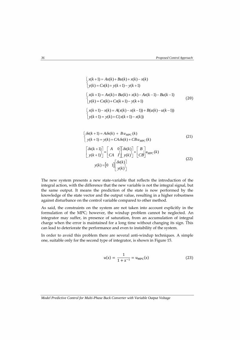
As said, the constraints on the system are not taken into account explicitly in the formulation of the MPC; however, the windup problem cannot be neglected. An integrator may suffer, in presence of saturation, from an accumulation of integral charge when the error is maintained for a long time without changing its sign. This can lead to deteriorate the performance and even to instability of the system.
In order to avoid this problem there are several anti-windup techniques. A simple one, suitable only for the second type of integrator, is shown in Figure 15.
( )
( ) ( )
Proposed Control Approach 37
Model Predictive Control for Multi-Phase Buck Converter with Variable Output Voltage
Without considering the saturation, it is possible to write the transfer function of the system according to the block rules that leads to the same expression of the non-strictly proper integral action in (18). It means that the two systems are equivalent, but the second formulation has the advantage to avoid the windup.
Considering the system in saturation and considering that the variable v is equal to u delayed by one step it is possible to write the equations (24).
( )
It means that even if the error (in this case the control action of the MPC) remains positive after saturation has been reached, there is no integral charge and both variable v and u stay limited. So when the error changes its sign the control promptly reduce the control action.
( ) ( )
( )
( )
III. State reference tracking
The MPC hides a first problem in the use of all the state variables in order to evaluate the prediction of the output variable. In general this problem is solved with the use of a Kalman filter that is able to give an estimation of all the state variables knowing only the output one. A question at this point could be whether it is convenient to measure all the state variables to control only the output one. It may be more suitable
z
z-1
1
z
++
umpcu u'
u'umpc u
Without Anti wind-up
With anti wind-up
Figure 15: Anti wind-up integral action
38 Proposed Control Approach
Model Predictive Control for Multi-Phase Buck Converter with Variable Output Voltage
to exploit all the information in a better way, for instance using not only the knowledge of the state to predict the output, but also trying to control all the state variables as in the optimum control. In this way we should be able to control completely the behavior of the plant.
The approach consists of controlling all the state variables, assigning them a proper reference so that it is possible to reach a better performance in terms of speed and behavior of the system. The difficult part of this approach is to define a value for each variable.
The idea to give a reference to each state variable leads to a new formulation of the cost function, where the error is defined as the difference between the state reference and the state variables.
)()()( ikxikxike
( )
The open loop method is used for the prediction of the state resulting in the expression in (26).
)1(
)(
1
00
)(
)(
)1(
Nku
ku
BBnA
B
kxnA
A
Nkx
kx
( )
)()()1( kUs
Bkxs
AkX
After the minimization of the cost function we finally obtain the close form of the new control law (27).
PlantKMPC
AOL
Future
Referenceyout
State
Variables
Figure 16: MPC Scheme
Proposed Control Approach 39
Model Predictive Control for Multi-Phase Buck Converter with Variable Output Voltage
)()1()( kxAkXKkU smpc
( )
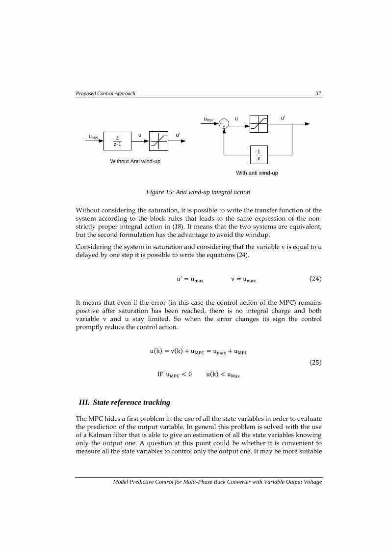
Figure 16 shows the control scheme of the two approaches outlined in this chapter. The differences are in the definition of the OL and control gain matrices. In the output reference scheme only the prediction of the output is performed and is compared with its future reference. In the state reference approach AOL gives a prediction of the entire state vector and consequently also a reference for all the state variables is required. The increased complexity for the second solution is justified by the possibility to decrease the prediction horizon in order to get the same result than the first approach.
There are two problems still to be solved for a perfect functioning of the system: the definition of the state reference and the feasibility problem of the control.
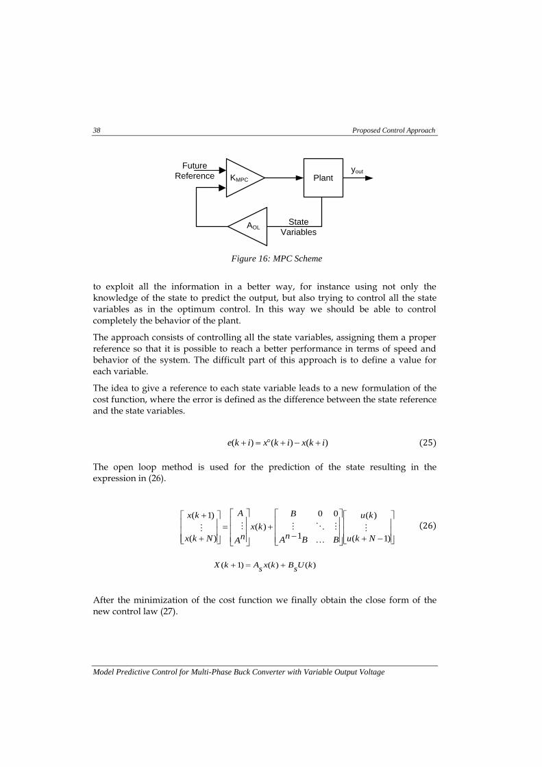
When we have to define a reference for the state variable we face the problem of choosing the best solution to improve the output behavior. There are several methods to generate a state reference by the output one. Many methods imply high computation cost and, for this reason, do not represent an attractive solution to our problem. Most are based on the knowledge of the system and hence increase the sensibility toward possible changes of the plant. Here it is presented a simple but effective method to generate the state reference that should overcome these limits. It is based on the formulation of the system model in δ-transform (19), and in the implementation of the proper integral action (18) as part of the system.
Several methods have been presented in literature. One way is to generate a multi-dimensional reference trajectory from a scalar input command using the model of a switching circuit in conjunction with a feedback algorithm [Doug’97]. The algorithm generates the state references simulating in line the digital model of the system controlled by any control law. This method is not appropriate for this case, because extremely complex in terms of realizations and computing power.
Output
Voltage
MPCz
1
z
1
Vo
Buck
Converter
Delay Compensator
Kalman
Predictor
Voltage
reference
Figure 17: Overall Control scheme with integral action
40 Proposed Control Approach
Model Predictive Control for Multi-Phase Buck Converter with Variable Output Voltage
A second method is based on the equivalence between a first order difference system equations and input-output mapping [Mariethoz’08]. Because of this equivalence, it is possible, in single-input single-output (SISO) system, extracting the knowledge of the state variables by the knowledge of n consecutive values of the output and n-1 consecutive value of the input, where n defines the order of the system. In case of the Buck converter, the value of the current can be extract by the knowledge of two consecutive values of the capacitor voltage and the duty cycle.
The second method presents at least two disadvantages. Although it is simpler than the previous one, it requires an additional operation in line to obtain the current reference. Second, it is affected by disturbances on the control variable. Since the solution is based on the knowledge of load, if the load changes, the method cannot guarantee a good reference of the current inductor anymore.
There are considerable advantages in this method. First, the definition of the reference does not depend on the knowledge of the system; it means that this method is not affected by system changes. It is an important advantage that gives more generality to the solution. We shall consider, for instance, the case of the Buck converter. The load is part of the system, so we model the converter assuming that we know the value of the load. In the same way, with the previous method, we define a reference for the output current based on the nominal value of the load resistance but if it varies the reference defection based on the model would be incorrect. However, with the description model based on δ-transform we can define a reference value for the current that is correct for any change of the load, since at steady state the difference between two consecutive samples needs to be zero regardless of the load. Another important advantage is the simplicity. In fact it does not require any additional calculation. Compared with the previous solutions the computational cost is zero.
If for constant references this method works perfectly, in case of sinusoidal reference tracking, the difference between two consecutive values is not zero. However, if the
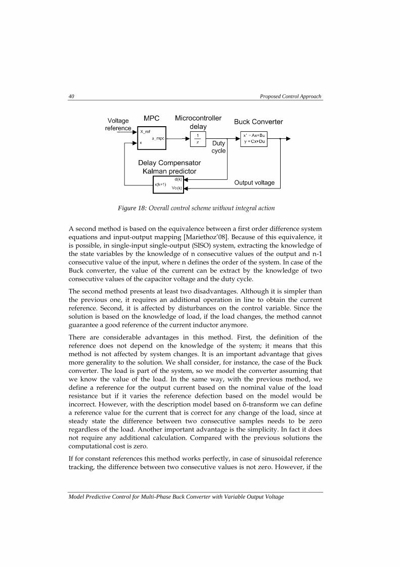
Figure 18: Overall control scheme without integral action
Proposed Control Approach 41
Model Predictive Control for Multi-Phase Buck Converter with Variable Output Voltage
sampling frequency is much higher than the sinusoidal frequency, as the case of SMPS, this assumption can be still valid. Besides, setting the state reference to zero, this method makes the entire system more robust. Finally the method seems to fit better with the requirements specified for the application.
IV. Delay compensator
Both approaches require the knowledge of the state variable in order to perform the OL prediction. In case of a MP Buck converter it means to sense both output capacitor voltage and the sum of all the phase currents. However sensing the current at high sampling frequency is in general more demanding than the measurement of the voltage. Alternatively, it is possible to use a Kalman filter in order to have an estimation of the state variables. This solution is largely used especially when there are more than two state variables since it is not always possible to have access to all the all of them by measurement. In this case the Kalman filter provides also another advantage in terms of robustness of the first prediction step.
Figure 18 shows a more detailed schematic of the control system, where a digital delay of one step appears in series with the MPC block. Although a liner control has
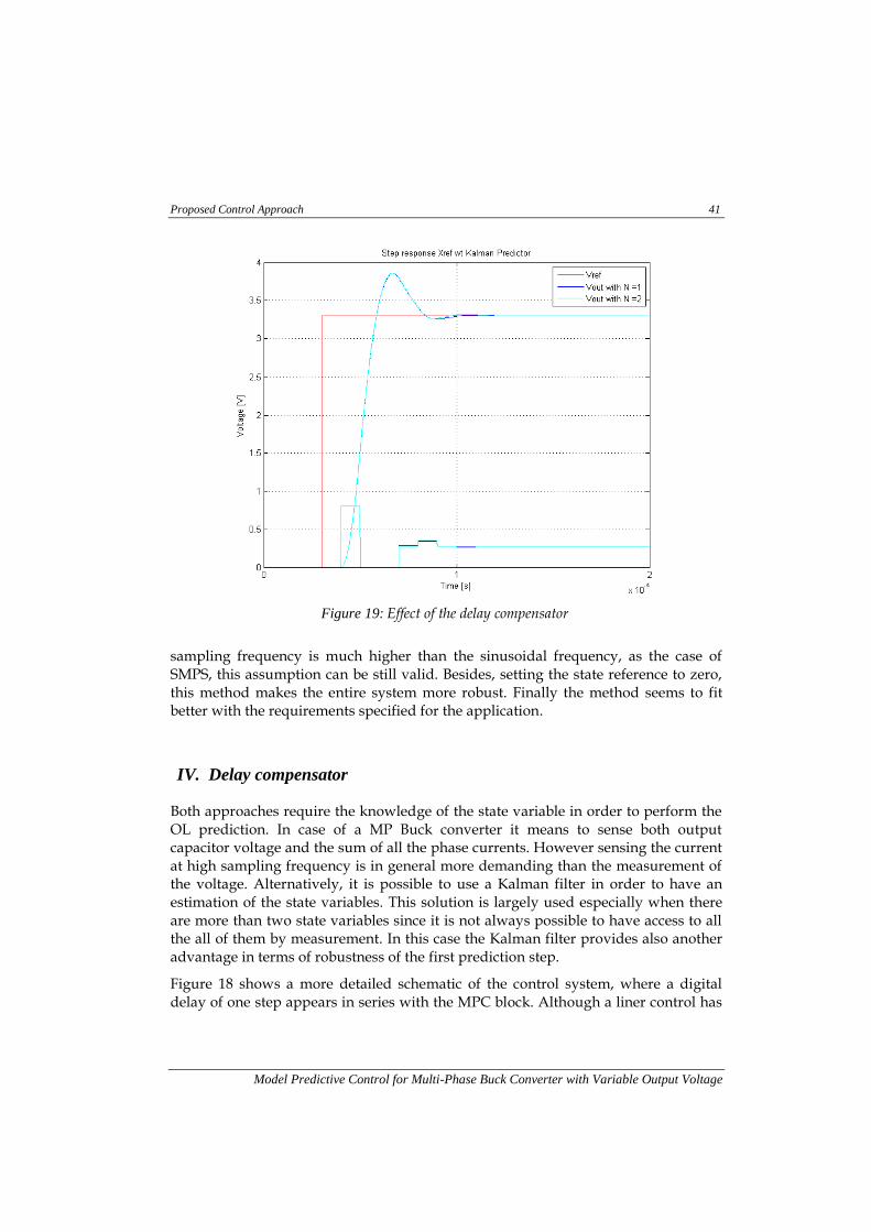
Figure 19: Effect of the delay compensator
42 Proposed Control Approach
Model Predictive Control for Multi-Phase Buck Converter with Variable Output Voltage
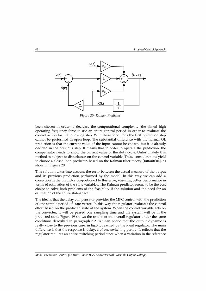
been chosen in order to decrease the computational complexity, the aimed high operating frequency force to use an entire control period in order to evaluate the control action for the following step. With these conditions the first prediction step cannot be performed in open loop. The substantial difference with the normal OL prediction is that the current value of the input cannot be chosen, but it is already decided in the previous step. It means that in order to operate the prediction, the compensator needs to know the current value of the duty cycle. Unfortunately this method is subject to disturbance on the control variable. These considerations yield to choose a closed loop predictor, based on the Kalman filter theory [Bittanti’04], as shown in Figure 20.
This solution takes into account the error between the actual measure of the output and its previous prediction performed by the model. In this way we can add a correction in the predictor proportioned to this error, ensuring better performance in terms of estimation of the state variables. The Kalman predictor seems to be the best choice to solve both problems of the feasibility if the solution and the need for an estimation of the entire state-space.
The idea is that the delay compensator provides the MPC control with the prediction of one sample period of state vector. In this way the regulator evaluates the control effort based on the predicted state of the system. When the control variable acts on the converter, it will be passed one sampling time and the system will be in the predicted state. Figure 19 shows the results of the overall regulator under the same conditions described in paragraph 3.2. We can notice that the output dynamic is really close to the previous case, in fig.3.5, reached by the ideal regulator. The main difference is that the response is delayed of one switching period. It reflects that the regulator requires an entire switching period since when a variation in the reference
L
Bd
Ad
+
++
1
z
X(k+1)
X(k)Cd
-+
y(k)
y(k)
u(k)
Figure 20: Kalman Predictor

Proposed Control Approach 43
Model Predictive Control for Multi-Phase Buck Converter with Variable Output Voltage
is noticed and an effect on the control variable is produced. The overall system with the compensator delay result to be asymptotically stable.

Control Architecture 45
Model Predictive Control for Multi-Phase Buck Converter with Variable Output Voltage
Chapter: 3 Control Architecture
In the previous chapter, two different approaches have been introduced able to use the future information of the reference supposed to be known in advance. The controller described in Chapter 2 has been implemented on a FPGA Spartan 3 of Xilinx. In this chapter the overall architecture is described as well as some implementation issues and the new digital modulator used to drive the four-phase converter.
I. Regulator Design
A GA [Goldberg’89] is a heuristic search that belongs to the larger class of Evolutionary Algorithm (EA). EA is a subset of optimization algorithms that have in common some mechanisms inspired by biological evolution, such as: reproduction, mutation, recombination, and selection. All the possible solutions of the optimization problem play the role of individuals in a population. At each problem is associated a cost function that assigns a value to each solution, called fitness. This value represents how well the solution for the problem is. If the fitness is higher as better is the solution, EA will look for the individual with the highest one, otherwise the algorithm will try to minimize it.
From an initial set of individuals new generations are obtained combining the best individuals according to the mechanism of evolution. After some generations the best individual will be selected by EA as best solution to the problem.
In GA the candidate solution (called phenotype or individuals) is encoded in a string (called genotype or chromosomes). The string can be codified in bits of natural or real number. The evolution usually starts from a population randomly generated in order to have a heterogeneous set of individuals, which can guarantee fast performances in the search of the solution.
At each generation, the fitness of every individual is evaluated according a proper function. After this, multiple individuals are stochastically selected from the current population and modified to form a new population. The idea is to select the best solutions of each generation and combine them to form better ones. However, the selection is performed stochastically, giving more possibility to be selected to the better solutions, but it is important that also the worse have possibility in order to avoid local optimum. The recombination is carried out with two mechanism again inspired by the nature: crossover and mutation.
46 Control Architecture
Model Predictive Control for Multi-Phase Buck Converter with Variable Output Voltage
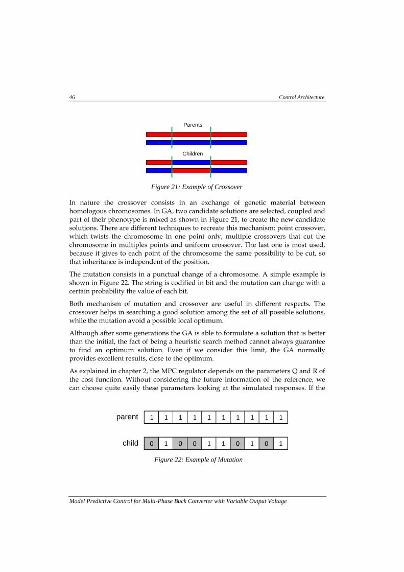
In nature the crossover consists in an exchange of genetic material between homologous chromosomes. In GA, two candidate solutions are selected, coupled and part of their phenotype is mixed as shown in Figure 21, to create the new candidate solutions. There are different techniques to recreate this mechanism: point crossover, which twists the chromosome in one point only, multiple crossovers that cut the chromosome in multiples points and uniform crossover. The last one is most used, because it gives to each point of the chromosome the same possibility to be cut, so that inheritance is independent of the position.
The mutation consists in a punctual change of a chromosome. A simple example is shown in Figure 22. The string is codified in bit and the mutation can change with a certain probability the value of each bit.
Both mechanism of mutation and crossover are useful in different respects. The crossover helps in searching a good solution among the set of all possible solutions, while the mutation avoid a possible local optimum.
Although after some generations the GA is able to formulate a solution that is better than the initial, the fact of being a heuristic search method cannot always guarantee to find an optimum solution. Even if we consider this limit, the GA normally provides excellent results, close to the optimum.
As explained in chapter 2, the MPC regulator depends on the parameters Q and R of the cost function. Without considering the future information of the reference, we can choose quite easily these parameters looking at the simulated responses. If the
Parents
Children
Figure 21: Example of Crossover
1 1 1 1 1 1 1 1 1 1
0 1 0 0 1 1 0 1 0 1
parent
child
Figure 22: Example of Mutation
Control Architecture 47
Model Predictive Control for Multi-Phase Buck Converter with Variable Output Voltage
closed loop system is slow, it is possible to increase the bandwidth by increasing the parameter Q; if the control effort is high we can decrease it by setting a higher value for the parameter R. In this application we want something more. We would like to use the future information of the output reference to get some benefits in the reference tracking. At this stage the key point in the design is to get a good balance between the coefficients Q and R to weight the predictive error and the actual one. With the first term we try to anticipate the control action in order to reduce the phase delay between output and reference.
The manual design is appropriate to create good regulators for the classical case, but when we try to take advantage of future reference knowledge this assignation becomes more difficult and time-consuming because it is not completely clear how to modify the parameter, in order to reach the best performance. For these reasons I tried to find a solution for this problem using an advanced method of search as the genetic algorithm.
The MPC parameters are naturally encoded in a chromosome on real numbers while for the fitness there are at least two options. One possibility is given by the assignation of the dynamic. It means, for instance, trying to find the parameters that yield to specified closed loop poles. In this case, the fitness of each solution can be defined as the difference between the desired closed loop eigenvalues and the ones obtained by the solution (28). The GA can find a good set of parameters trying to minimize the fitness of the individuals.
| ( )| | ( )| ( )
The main advantage of this method consists of the possibility to specify overshoot and bandwidth of the closed loop transfer function.
A second idea consists on simulating the control law given by each solution and comparing the output waveform with the reference. In this case, we define the fitness as the quadratic sum of the difference between the reference and the output at each time (29).
∑( ( ) ( ))
( )
Therefore, by minimizing the fitness the GA is able to find the set of parameters that better tracks the reference.
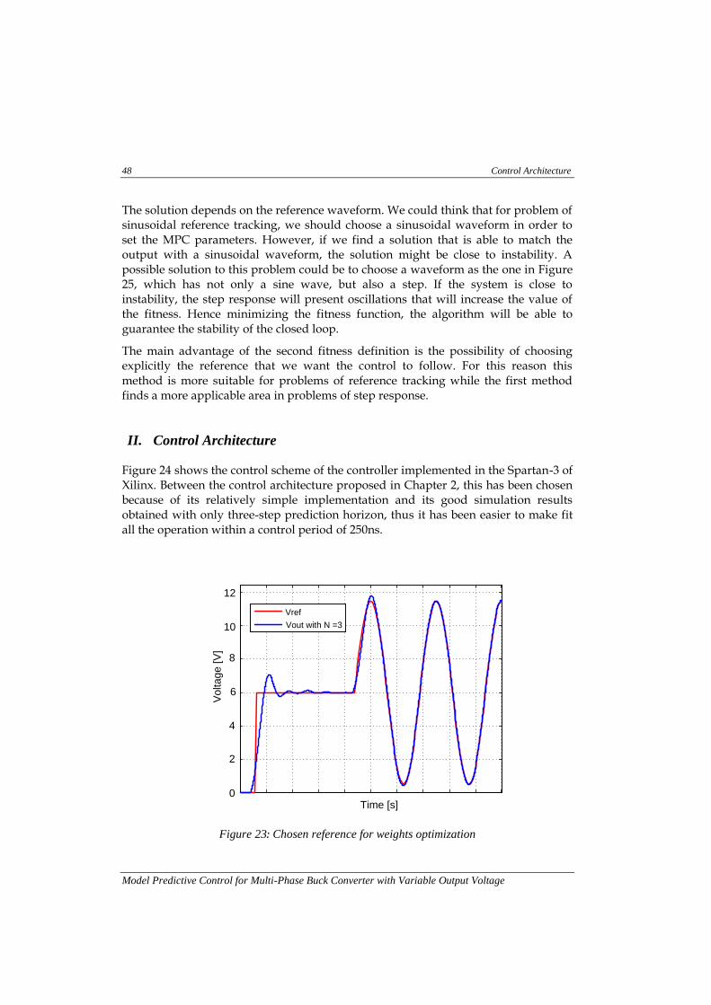
48 Control Architecture
Model Predictive Control for Multi-Phase Buck Converter with Variable Output Voltage
The solution depends on the reference waveform. We could think that for problem of sinusoidal reference tracking, we should choose a sinusoidal waveform in order to set the MPC parameters. However, if we find a solution that is able to match the output with a sinusoidal waveform, the solution might be close to instability. A possible solution to this problem could be to choose a waveform as the one in Figure 25, which has not only a sine wave, but also a step. If the system is close to instability, the step response will present oscillations that will increase the value of the fitness. Hence minimizing the fitness function, the algorithm will be able to guarantee the stability of the closed loop.
The main advantage of the second fitness definition is the possibility of choosing explicitly the reference that we want the control to follow. For this reason this method is more suitable for problems of reference tracking while the first method finds a more applicable area in problems of step response.
II. Control Architecture
Figure 24 shows the control scheme of the controller implemented in the Spartan-3 of Xilinx. Between the control architecture proposed in Chapter 2, this has been chosen because of its relatively simple implementation and its good simulation results obtained with only three-step prediction horizon, thus it has been easier to make fit all the operation within a control period of 250ns.
0
2
4
6
8
10
12
Vo
lta
ge
[V
]
Vref
Vout with N =3
Time [s]
Figure 23: Chosen reference for weights optimization
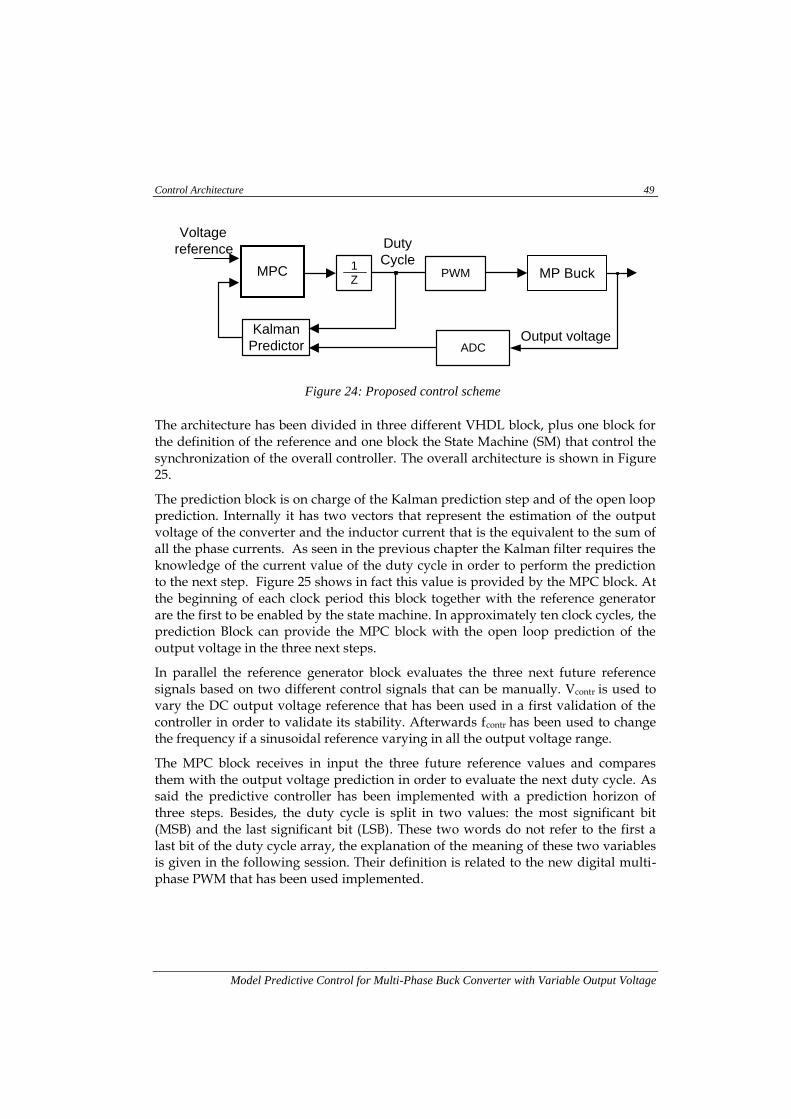
Control Architecture 49
Model Predictive Control for Multi-Phase Buck Converter with Variable Output Voltage
The architecture has been divided in three different VHDL block, plus one block for the definition of the reference and one block the State Machine (SM) that control the synchronization of the overall controller. The overall architecture is shown in Figure 25.
The prediction block is on charge of the Kalman prediction step and of the open loop prediction. Internally it has two vectors that represent the estimation of the output voltage of the converter and the inductor current that is the equivalent to the sum of all the phase currents. As seen in the previous chapter the Kalman filter requires the knowledge of the current value of the duty cycle in order to perform the prediction to the next step. Figure 25 shows in fact this value is provided by the MPC block. At the beginning of each clock period this block together with the reference generator are the first to be enabled by the state machine. In approximately ten clock cycles, the prediction Block can provide the MPC block with the open loop prediction of the output voltage in the three next steps.
In parallel the reference generator block evaluates the three next future reference signals based on two different control signals that can be manually. Vcontr is used to vary the DC output voltage reference that has been used in a first validation of the controller in order to validate its stability. Afterwards fcontr has been used to change the frequency if a sinusoidal reference varying in all the output voltage range.
The MPC block receives in input the three future reference values and compares them with the output voltage prediction in order to evaluate the next duty cycle. As said the predictive controller has been implemented with a prediction horizon of three steps. Besides, the duty cycle is split in two values: the most significant bit (MSB) and the last significant bit (LSB). These two words do not refer to the first a last bit of the duty cycle array, the explanation of the meaning of these two variables is given in the following session. Their definition is related to the new digital multi-phase PWM that has been used implemented.
MPC
Duty
CycleMP Buck
Voltage
reference
Output voltageKalman
Predictor ADC
PWM1
Z
Figure 24: Proposed control scheme
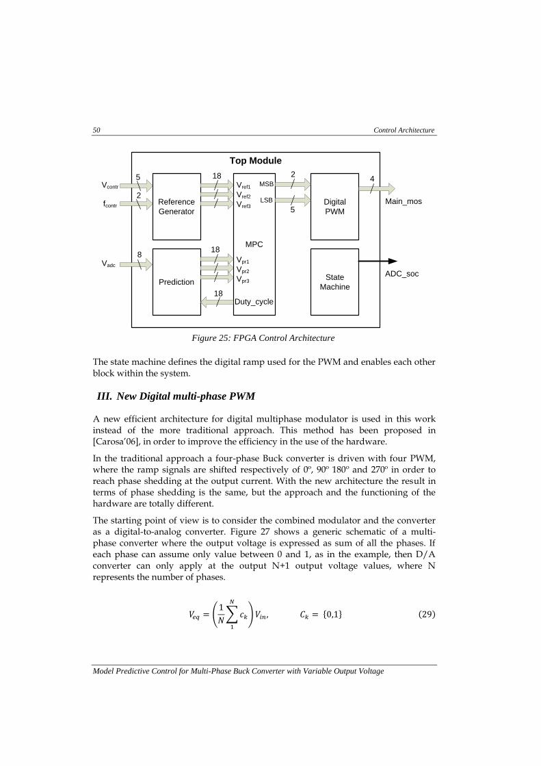
50 Control Architecture
Model Predictive Control for Multi-Phase Buck Converter with Variable Output Voltage
The state machine defines the digital ramp used for the PWM and enables each other block within the system.
III. New Digital multi-phase PWM
A new efficient architecture for digital multiphase modulator is used in this work instead of the more traditional approach. This method has been proposed in [Carosa’06], in order to improve the efficiency in the use of the hardware.
In the traditional approach a four-phase Buck converter is driven with four PWM, where the ramp signals are shifted respectively of 0º, 90º 180º and 270º in order to reach phase shedding at the output current. With the new architecture the result in terms of phase shedding is the same, but the approach and the functioning of the hardware are totally different.
The starting point of view is to consider the combined modulator and the converter as a digital-to-analog converter. Figure 27 shows a generic schematic of a multi-phase converter where the output voltage is expressed as sum of all the phases. If each phase can assume only value between 0 and 1, as in the example, then D/A converter can only apply at the output N+1 output voltage values, where N represents the number of phases.
(
∑
) ( )
Top Module
Digital
PWM
Prediction
8
MPC
Reference
Generator
State
Machine
Vadc
MSB
LSB
5
2
Vref1
Vref2
Vref3
18
18
Vpr1
Vpr2
Vpr3
4
Main_mos
Duty_cycle
18
ADC_soc
2
5Vcontr
fcontr
Figure 25: FPGA Control Architecture
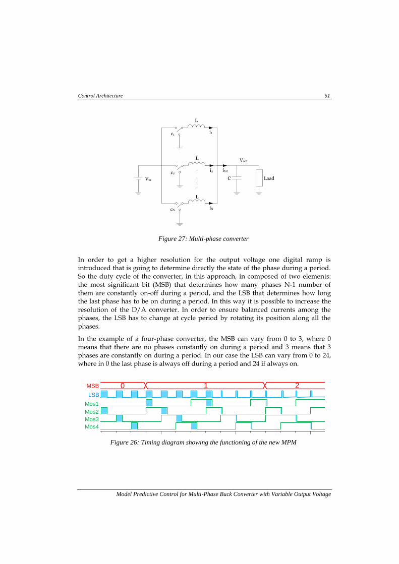
Control Architecture 51
Model Predictive Control for Multi-Phase Buck Converter with Variable Output Voltage
In order to get a higher resolution for the output voltage one digital ramp is introduced that is going to determine directly the state of the phase during a period. So the duty cycle of the converter, in this approach, in composed of two elements: the most significant bit (MSB) that determines how many phases N-1 number of them are constantly on-off during a period, and the LSB that determines how long the last phase has to be on during a period. In this way it is possible to increase the resolution of the D/A converter. In order to ensure balanced currents among the phases, the LSB has to change at cycle period by rotating its position along all the phases.
In the example of a four-phase converter, the MSB can vary from 0 to 3, where 0 means that there are no phases constantly on during a period and 3 means that 3 phases are constantly on during a period. In our case the LSB can vary from 0 to 24, where in 0 the last phase is always off during a period and 24 if always on.
Mos1
Mos2
Mos3
Mos4
MSB
LSB
Time
10 2
Figure 26: Timing diagram showing the functioning of the new MPM
Vin
L
C Load
L
L
i1
i2
iN
itot
c1
c2
cN
Vout
Figure 27: Multi-phase converter
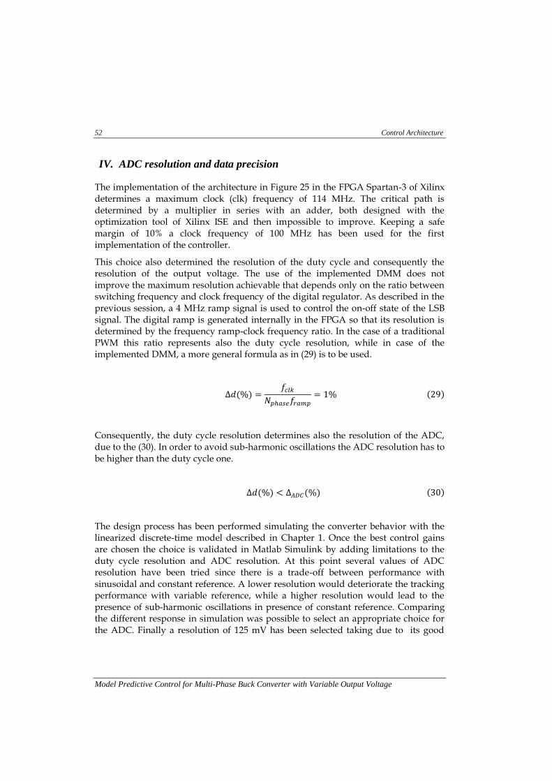
52 Control Architecture
Model Predictive Control for Multi-Phase Buck Converter with Variable Output Voltage
IV. ADC resolution and data precision
The implementation of the architecture in Figure 25 in the FPGA Spartan-3 of Xilinx determines a maximum clock (clk) frequency of 114 MHz. The critical path is determined by a multiplier in series with an adder, both designed with the optimization tool of Xilinx ISE and then impossible to improve. Keeping a safe margin of 10% a clock frequency of 100 MHz has been used for the first implementation of the controller.
This choice also determined the resolution of the duty cycle and consequently the resolution of the output voltage. The use of the implemented DMM does not improve the maximum resolution achievable that depends only on the ratio between switching frequency and clock frequency of the digital regulator. As described in the previous session, a 4 MHz ramp signal is used to control the on-off state of the LSB signal. The digital ramp is generated internally in the FPGA so that its resolution is determined by the frequency ramp-clock frequency ratio. In the case of a traditional PWM this ratio represents also the duty cycle resolution, while in case of the implemented DMM, a more general formula as in (29) is to be used.
( )
( )
Consequently, the duty cycle resolution determines also the resolution of the ADC, due to the (30). In order to avoid sub-harmonic oscillations the ADC resolution has to be higher than the duty cycle one.
( ) ( ) ( )
The design process has been performed simulating the converter behavior with the linearized discrete-time model described in Chapter 1. Once the best control gains are chosen the choice is validated in Matlab Simulink by adding limitations to the duty cycle resolution and ADC resolution. At this point several values of ADC resolution have been tried since there is a trade-off between performance with sinusoidal and constant reference. A lower resolution would deteriorate the tracking performance with variable reference, while a higher resolution would lead to the presence of sub-harmonic oscillations in presence of constant reference. Comparing the different response in simulation was possible to select an appropriate choice for the ADC. Finally a resolution of 125 mV has been selected taking due to its good
Control Architecture 53
Model Predictive Control for Multi-Phase Buck Converter with Variable Output Voltage
response in simulation and because the corresponding data representation can be process in easier way compared with the one of other resolution.
A fix-point data representation has been used for its simplicity and low computational cost. In the attempt to fit all the operations within the control period of 250 ns, all the possible simplifications have been performed in order to decrease the complexity of the controller. In this way a simpler representation of the number within the FPGA can diminish the time for data conversion and for the data processing. In particular with a unsigned representation of the output voltage in the ADC with 8 bits and a resolution of 125 mV, output voltage at 1 V is represented by the sequence 00001000. This number in order to be used by the FPGA has to be converted to a representation at 18 bits, with 12 bits for the decimal part and 6 for the integer. In this case the conversion is quite easy and consist s of simply adding some zeros to the number, with a remarkable simplification of the data conversion. Another ADC resolution would imply a different representation of the output voltage and a more demanding data processing.

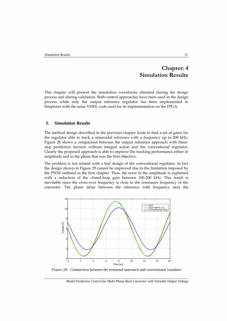
Simulation Results 55
Model Predictive Control for Multi-Phase Buck Converter with Variable Output Voltage
Chapter: 4 Simulation Results
This chapter will present the simulation waveforms obtained during the design process and during validation. Both control approaches have been used in the design process while only the output reference regulator has been implemented in Simplorer with the same VHDL code used for its implementation on the FPGA.
I. Simulation Results
The method design described in the previous chapter leads to find a set of gains for the regulator able to track a sinusoidal reference with a frequency up to 200 kHz. Figure 28 shows a comparison between the output reference approach with three-step prediction horizon without integral action and the conventional regulator. Clearly the proposed approach is able to improve the tracking performance either in amplitude and in the phase that was the first objective.
The problem is not related with a bed design of the conventional regulator. In fact the design shown in Figure 29 cannot be improved due to the limitation imposed by the PWM outlined in the first chapter. Thus, the error in the amplitude is explained with a reduction of the closed-loop gain between 100-200 kHz. This result is inevitable since the cross-over frequency is close to the resonance frequency of the converter. The phase delay between the reference with frequency near the
0
2
4
6
8
10
12
Vo
lta
ge
[V
]
VrefVout with N =3Conventional Reg
0 2 4 6 8 10 12 14 16
Time [us]
Figure 28: Comparison between the proposed approach and conventional regulator
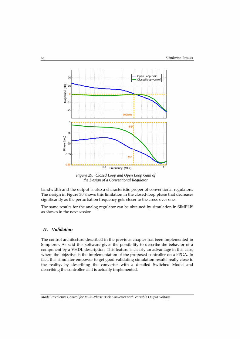
56 Simulation Results
Model Predictive Control for Multi-Phase Buck Converter with Variable Output Voltage
bandwidth and the output is also a characteristic proper of conventional regulators. The design in Figure 30 shows this limitation in the closed-loop phase that decreases significantly as the perturbation frequency gets closer to the cross-over one.
The same results for the analog regulator can be obtained by simulation in SIMPLIS as shown in the next session.
II. Validation
The control architecture described in the previous chapter has been implemented in Simplorer. As said this software gives the possibility to describe the behavior of a component by a VHDL description. This feature is clearly an advantage in this case, where the objective is the implementation of the proposed controller on a FPGA. In fact, this simulator empower to get good validating simulation results really close to the reality, by describing the converter with a detailed Switched Model and describing the controller as it is actually implemented.
Frequency (MHz)
0.1 1-180
-135
-90
-45
0
Ph
ase
(d
eg
)
-20
-10
0
10
20
Ma
gn
itu
de
(d
B)
300kHz
63º
-58º
Open Loop Gain
Closed loop vo/vref
Figure 29: Closed Loop and Open Loop Gain of
the Design of a Conventional Regulator
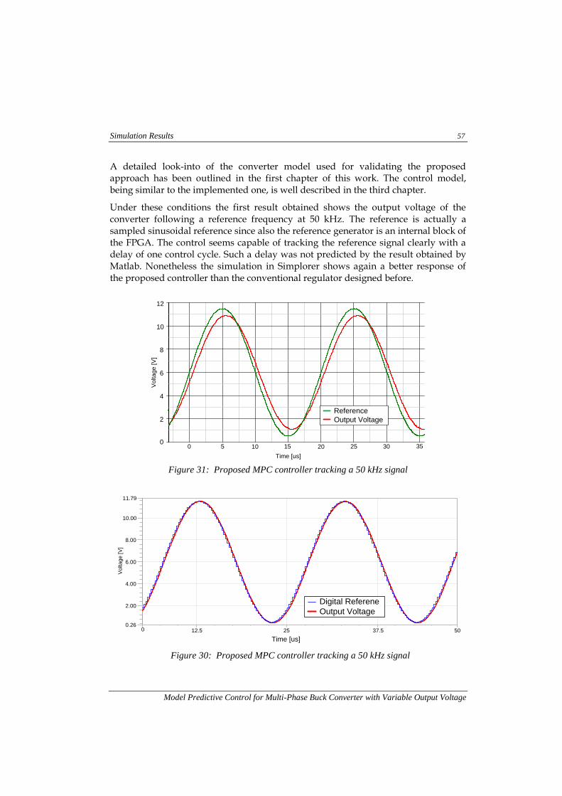
Simulation Results 57
Model Predictive Control for Multi-Phase Buck Converter with Variable Output Voltage
A detailed look-into of the converter model used for validating the proposed approach has been outlined in the first chapter of this work. The control model, being similar to the implemented one, is well described in the third chapter.
Under these conditions the first result obtained shows the output voltage of the converter following a reference frequency at 50 kHz. The reference is actually a sampled sinusoidal reference since also the reference generator is an internal block of the FPGA. The control seems capable of tracking the reference signal clearly with a delay of one control cycle. Such a delay was not predicted by the result obtained by Matlab. Nonetheless the simulation in Simplorer shows again a better response of the proposed controller than the conventional regulator designed before.
0 12.5 25 37.5 50
Time [us]
0.26
2.00
4.00
6.00
8.00
10.00
11.79
Vo
lta
ge
[V
]
Digital Referene
Output Voltage
Figure 30: Proposed MPC controller tracking a 50 kHz signal
0 5 10 15 20 25 30 35
Time [us]
0
2
4
6
8
10
12
Vo
lta
ge
[V
]
Reference
Output Voltage
Figure 31: Proposed MPC controller tracking a 50 kHz signal
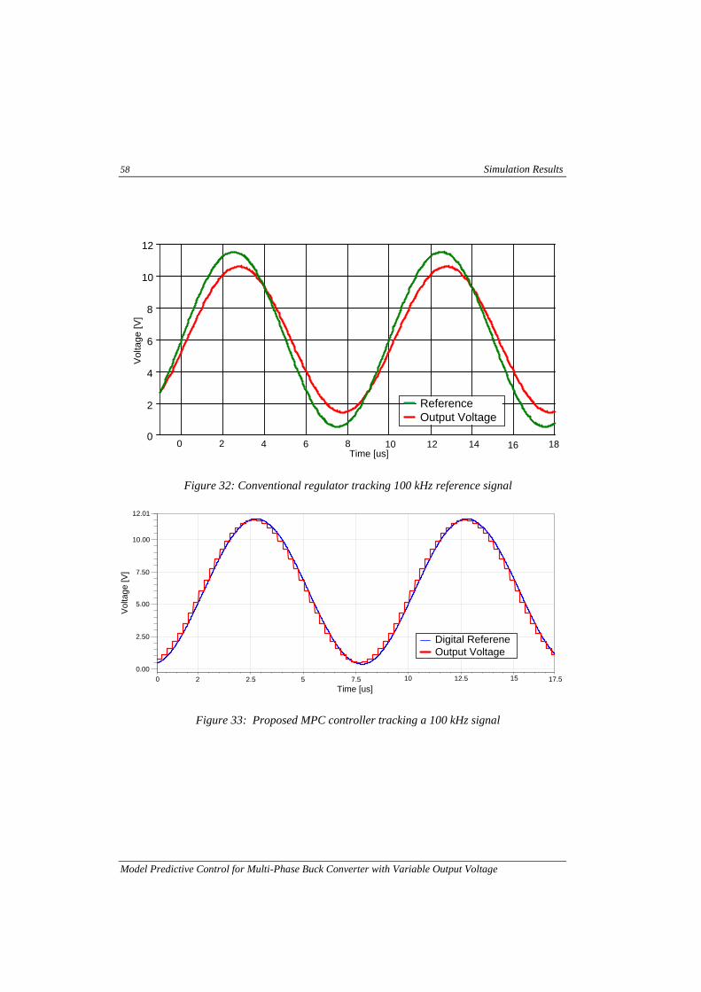
58 Simulation Results
Model Predictive Control for Multi-Phase Buck Converter with Variable Output Voltage
0
2
4
6
8
10
12
Vo
lta
ge
[V
]
0 2 4 6 8 10 12 14 16 18Time [us]
Reference
Output Voltage
Figure 32: Conventional regulator tracking 100 kHz reference signal
0 2 2.5 5 7.5 10 12.5 15 17.5
Time [us]
0.00
2.50
5.00
7.50
10.00
12.01
Vo
lta
ge
[V
]
Digital Referene
Output Voltage
Figure 33: Proposed MPC controller tracking a 100 kHz signal
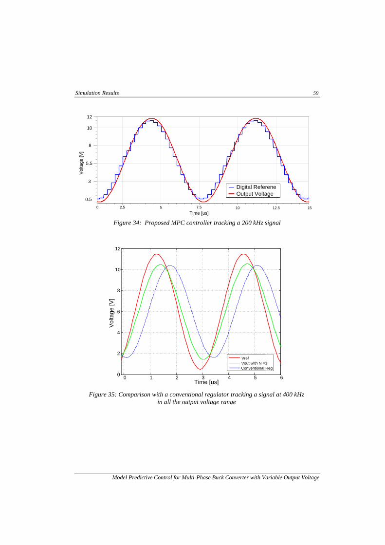
Simulation Results 59
Model Predictive Control for Multi-Phase Buck Converter with Variable Output Voltage
0 2.5 5 7.5 10 12.5 15
Time [us]
0.5
3
5.5
8
10
12
Vo
lta
ge
[V
]
Digital Referene
Output Voltage
Figure 34: Proposed MPC controller tracking a 200 kHz signal
0 1 2 3 4 5 60
2
4
6
8
10
12
Time [us]
Vo
lta
ge
[V
]
Vref
Vout with N =3
Conventional Reg
Figure 35: Comparison with a conventional regulator tracking a signal at 400 kHz
in all the output voltage range
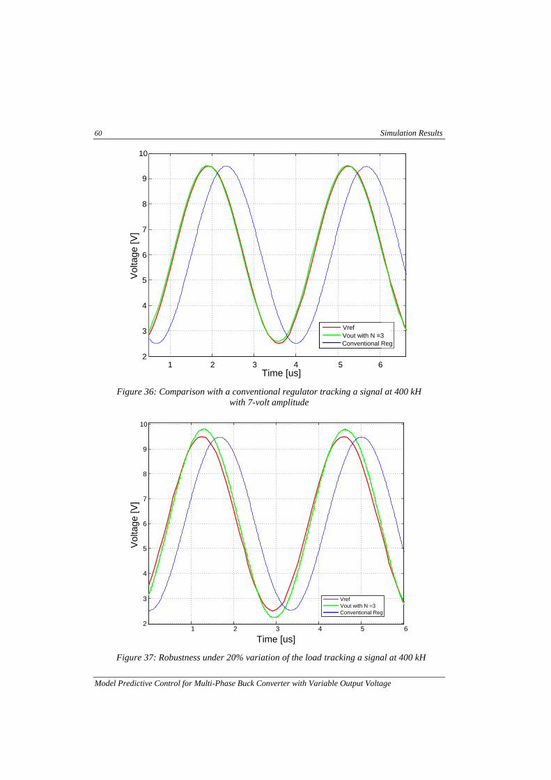
60 Simulation Results
Model Predictive Control for Multi-Phase Buck Converter with Variable Output Voltage
2
3
4
5
6
7
8
9
10
Vo
lta
ge
[V
]
Vref
Vout with N =3
Conventional Reg
1 2 3 4 5 6Time [us]
Figure 36: Comparison with a conventional regulator tracking a signal at 400 kH
with 7-volt amplitude
1 2 3 4 5 62
3
4
5
6
7
8
9
10
Time [us]
Vo
lta
ge
[V
]
Vref
Vout with N =3
Conventional Reg
Figure 37: Robustness under 20% variation of the load tracking a signal at 400 kH
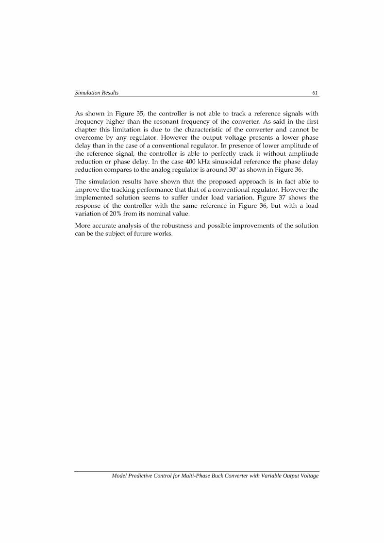
Simulation Results 61
Model Predictive Control for Multi-Phase Buck Converter with Variable Output Voltage
As shown in Figure 35, the controller is not able to track a reference signals with frequency higher than the resonant frequency of the converter. As said in the first chapter this limitation is due to the characteristic of the converter and cannot be overcome by any regulator. However the output voltage presents a lower phase delay than in the case of a conventional regulator. In presence of lower amplitude of the reference signal, the controller is able to perfectly track it without amplitude reduction or phase delay. In the case 400 kHz sinusoidal reference the phase delay reduction compares to the analog regulator is around 30º as shown in Figure 36.
The simulation results have shown that the proposed approach is in fact able to improve the tracking performance that that of a conventional regulator. However the implemented solution seems to suffer under load variation. Figure 37 shows the response of the controller with the same reference in Figure 36, but with a load variation of 20% from its nominal value.
More accurate analysis of the robustness and possible improvements of the solution can be the subject of future works.

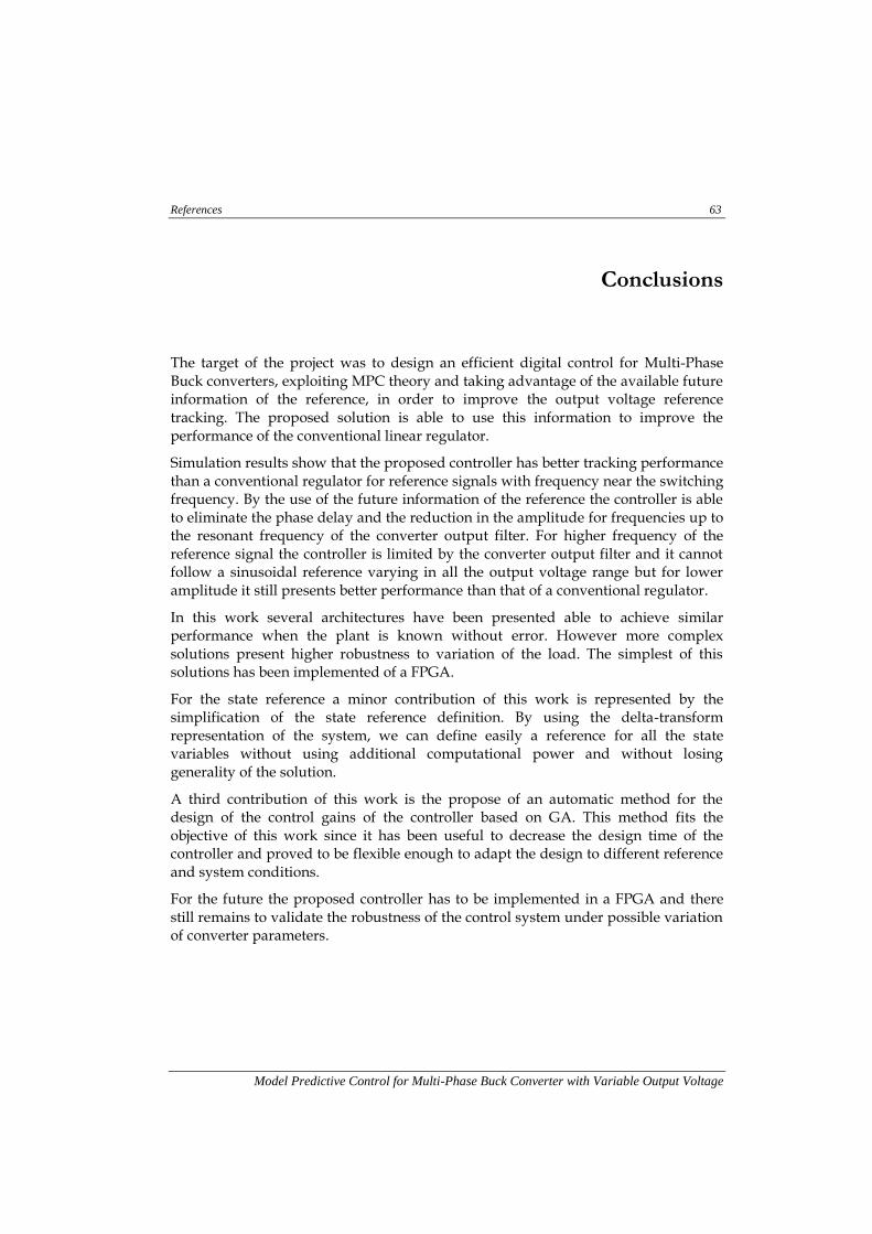
References 63
Model Predictive Control for Multi-Phase Buck Converter with Variable Output Voltage
Conclusions
The target of the project was to design an efficient digital control for Multi-Phase Buck converters, exploiting MPC theory and taking advantage of the available future information of the reference, in order to improve the output voltage reference tracking. The proposed solution is able to use this information to improve the performance of the conventional linear regulator.
Simulation results show that the proposed controller has better tracking performance than a conventional regulator for reference signals with frequency near the switching frequency. By the use of the future information of the reference the controller is able to eliminate the phase delay and the reduction in the amplitude for frequencies up to the resonant frequency of the converter output filter. For higher frequency of the reference signal the controller is limited by the converter output filter and it cannot follow a sinusoidal reference varying in all the output voltage range but for lower amplitude it still presents better performance than that of a conventional regulator.
In this work several architectures have been presented able to achieve similar performance when the plant is known without error. However more complex solutions present higher robustness to variation of the load. The simplest of this solutions has been implemented of a FPGA.
For the state reference a minor contribution of this work is represented by the simplification of the state reference definition. By using the delta-transform representation of the system, we can define easily a reference for all the state variables without using additional computational power and without losing generality of the solution.
A third contribution of this work is the propose of an automatic method for the design of the control gains of the controller based on GA. This method fits the objective of this work since it has been useful to decrease the design time of the controller and proved to be flexible enough to adapt the design to different reference and system conditions.
For the future the proposed controller has to be implemented in a FPGA and there still remains to validate the robustness of the control system under possible variation of converter parameters.
64 References
Model Predictive Control for Multi-Phase Buck Converter with Variable Output Voltage
References
[Beccuti’09] Beccuti, A.G.; Mariethoz, S.; Cliquennois, S.; Shu Wang; Morari, M.; , "Explicit Model Predictive Control of DC–DC Switched-Mode Power Supplies With Extended Kalman Filtering," Industrial Electronics, IEEE Transactions on , vol.56, no.6, pp.1864-1874, June 2009
[Bittanti’04] Bittanti, S., “Theory of Prediction and Filtering”, PitagoraEditrice, Bologna, 2004
[Bolzern’09] Bolzern, P., Scattolini, R. “ Fundamentos de control automático”, 3° Ed., McGraw-Hill, Milano, 2009.
[Canalli’96] Canalli, V.M., Cobos, J.A., Oliver, J.A., Uceda, J., “Behavioral large signal averaged model for DC/DC switching power converters”, Proceedings of Power Electronics Specialists Conference, 1996. PESC '96
[Carosa’06] Carosa, T.; Zane, R.; Maksimovic, D.; , "Digital Multiphase Modulator — A Power D/A Perspective," Power Electronics Specialists Conference, 2006. PESC '06. 37th IEEE , vol., no., pp. 1- 6, 18-22 June 2006
[Choi’05] Choi, K., Soma, R., Pedram, M.: “Fine-Grained Dynamic Voltage and Frequency Scaling for Precise Energy and Performance Tradeoff Based on the Ratio of Off-Chip Access to On-Chip Computation Times”, IEEE trans. on computer-aided design of integrated circuits and systems, vol. 24, No. 1, Jan. 2005
[Doug’97] Doug, S and Ping, H., “Predictive Discrete Time Control Of Switch-mode Applications.” Power Electronics Specialists Conference, 1997. PESC '97, 28th Annual IEEE
[Goldberg’89] Goldberg, D. E, “Genetic Algorithms in Search Optimization and Machine Learning”, Addison, 1989
[Liupung’09] Liuping W., “Model Predictive Control System Design and Implementation Using MATLAB®”, Second E. Springer, 2009.
[Magni’01] Magni L., De Nicolao, G. and Scattolini, R., "Model predictive control: output feedback and tracking of nonlinear systems", in Nonlinear Model Predictive Control:
References 65
Model Predictive Control for Multi-Phase Buck Converter with Variable Output Voltage
Theory and Practice, B. Kouvaritakis e M. Cannon eds., IEEE Control Engineering Series 61
[Mariethoz’08] Mariethoz, S.; Beccuti, A.G.; Papafotiou, G.; Morari, M.; , "Sensorless explicit model predictive control of the DC-DC buck converter with inductor current limitation," Applied Power Electronics Conference and Exposition, 2008. APEC 2008. Twenty-Third Annual IEEE
[Mattavelli’06] Mattavelli P., Buso S., “Digital Control in Power Electronics”, Morgan & Claypool Publishers, 2006
[Middleton’90] Middleton, R, H, Goodwin, G. C., “Digital control and estimation”, Prentice Hall, 1990
[Oliver’00] Oliver, J.A., Cobos, J.A., Uceda, J., Rascon, M., Quinones, C., “Systematic approach for developing large-signal averaged models of multi-output PWM converters”, Proceedings of Power Electronics Specialists Conference, 2000. PESC
[Qiu’05] Yang Qiu; Ming Xu; Kaiwei Yao; Juanjuan Sun; Lee, F.C.; , "The multi-frequency small-signal model for buck and multiphase interleaving buck converters," Applied Power Electronics Conference and Exposition, 2005. APEC 2005. Twentieth Annual IEEE , vol.1, no., pp. 392- 398 Vol. 1, 6-10 March 2005
[Vasic’10] Miroslav, V., “Wide Bandwidth High Efficiency Power Converter for RF Amplifiers”, Doctoral thesis, UPM, ETSII, 2010.
Recommended


![[SAFE] - Suburban Areas Favoring Energy efficiency](https://img.pdfslide.tips/doc/110x75/62b32f11cbaa4b08b11941c3/safe-suburban-areas-favoring-energy-efficiency.jpg)