MORSE THEORYBY
J. MilnorBased on lecture notes by
M. SPIVAK and R. WELLS
ANNALS OF MATHEMATICS STUDIESPRINCETON UNIVERSITY PRESS
Annals of Mathematics Studies
Number 51


MORSE THEORYBY
J. MilnorBased on lecture notes by
M. SPIVAK and R. WELLS
PRINCETON, NEW JERSEY
PRINCETON UNIVERSITY PRESS
Copyright © 1963, © 1969, by Princeton University PressAll Rights ReservedL.C. Card 63-13729
ISBN 0-691-08008-9
Third Printing, with correctionsand a new Preface, 1969
Fourth Printing, 1970Fifth Printing, 1973
Printed in the United States of America

PREFACE
This book gives a present-day account of Marston Morse's theory of
the calculus of variations in the large. However, there have been im-
portant developments during the past few years which are not mentioned.
Let me describe three of these
R. Palais and S. Smale nave studied Morse theory for a real-valued
function on an infinite dimensional manifold and have given direct proofs
of the main theorems, without making any use of finite dimensional ap-
proximations. The manifolds in question must be locally diffeomorphic
to Hilbert space, and the function must satisfy a weak compactness con-
dition. As an example, to study paths on a finite dimensional manifold
M one considers the Hilbert manifold consisting of all absolutely con-
tinuous paths w: (0,11 - M with square integrable first derivative. Ac-
counts of this work are contained in R. Palais, Morse Theory on Hilbert
Manifolds, Topology, Vol. 2 (1963), pp. 299-340; and in S. Smale, Morse
Theory and a Non-linear Generalization of the Dirichlet Problem, Annals
of Mathematics, Vol. 8o (1964), pp. 382_396.
The Bott periodicity theorems were originally inspired by Morse
theory (see part IV). However, more elementary proofs, which do not in-
volve Morse theory at all, have recently been given. See M. Atiyah and
R. Bott, On the Periodicity Theorem for Complex Vector Bundles, Acts,
Mathematica, Vol. 112 (1964), pp. 229_247, as well as R. Wood, Banach
Algebras and Bott Periodicity, Topology, 4 (1965-66), pp. 371-389.
Morse theory has provided the inspiration for exciting developments
in differential topology by S. Smale, A. Wallace, and others, including
a proof of the generalized Poincare hypothesis in high dimensions. I
have tried to describe some of this work in Lectures on the h-cobordism
theorem, notes by L. Siebenmann and J. Sondow, Princeton University Press,
1965.
Let me take this opportunity to clarify one term which may cause con-
fusion. In §12 I use the word "energy" for the integral
v
vi PREFACE
1
E = s u at II2
at0
along a path w(t). V. Arnol'd points out to me that mathematicians for
the past 200 years have called E the "action"integral. This discrepancy
in terminology is caused by the fact that the integral can be interpreted,
in terms of a physical model, in more than one way.
Think of a particle P which moves along a surface M during the time
interval 0 < t < 1. 'Tie action of the particle during this time interval
is defined to be a certain constant times the integral E. If no forces
act on P (except for the constraining forces which hold it within M), then
the "principle of least action" asserts that E will be minimized within
the class of all paths joining w(0) to w(1), or at least that the first
variation of E will be zero. Hence P must traverse a geodesic.
But a quite different physical model is possible. Think of a rubber
band which is stretched between two points of a slippery curved surface.
If the band is described parametrically by the equation x = w(t), 0 < t
< 1, then the potential energy arising from tension will be proportional
to our integral E (at least to a first order of approximation). For an
equilibrium position this energy must be minimized, and hence the rubber
band will describe a geodesic.
The text which follows is identical with that of the first printing
except for a few corrections. I am grateful to V. Arnol'd, D. Epstein
and W. B. Houston, Jr. for pointing out corrections.
J.W.M.
Los Angeles, June 1968.
CONTENTS
PREFACE v
PART I. NON-DEGENERATE SMOOTH FUNCTIONS ON A MANIFOLD
§ 1 . Introduction . . . . . . . . . . . . . . . . . . . . . . . 1
§2. Definitions and Lemmas . . . . . . . . . . . . . . . . . . 4
§3. Homotopy Type in Terms of Critical Values . . . . . . . . 12
§4. Examples. . . . . . . . . . . . . . . . . . . . . . . . 25
§5. The Morse Inequalities . . . . . . . . . . . . . . . . . . 28
§6. Manifolds in Euclidean Space: The Existence of
Non-degenerate Functions . . . . . . . . . . . . . . . . . 32
§7. The Lefschetz Theorem on Hyperplane Sections. . . . . . . 39
PART II. A RAPID COURSE IN RIEMANNIAN GEOMETRY
§8. Covariant Differentiation . . . . . . . . . . . . . . . . 43
§9. The Curvature Tensor . . . . . . . . . . . . . . . . . . . 51
§10. Geodesics and Completeness . . . . . . . . . . . . . . . . 55
PART III. THE CALCULUS OF VARIATIONS APPLIED TO GEODESICS
§11. The Path Space of a Smooth Manifold . . . . . . . . . . . 67
§12. The Energy of a Path . . . . . . . . . . . . . . . . . . . 70
§13. The Hessian of the Energy Function at a Critical Path . . 74
§14. Jacobi Fields: The Null-space of E... . . . . . . . . . 77
§15. The Index Theorem . . . . . . . . . . . . . . . . . . . . 82
§16. A Finite Dimensional Approximation to sic . . . . . . . . 88
§17. The Topology of the Full Path Space . . . . . . . . . . . 93
§18. Existence of Non-conjugate Points . . . . . . . . . . . . 98
§19. Some Relations Between Topology and Curvature . . . . . . 100
vii
CONTENTS
PART IV. APPLICATIONS TO LIE GROUPS AND SYMMETFIC SPACES
§20. Symmetric Spaces . . . . . . . . . . . . . . . . . . . . log
§21. Lie Groups as Symmetric Spaces . . . . . . . . . . . . . 112
§22. Whole Manifolds of Minimal Geodesics . . . . . . . . . . 118
§23. The Bott Periodicity Theorem for the Unitary Group . . . 124
§24. The Periodicity Theorem for the Orthogonal Group. . . . . 133
APPENDIX. THE HOMOTOPY TYPE OF A MONOTONE UNION . . . . . . . . . . . 149
viii
PART I
NON-DEGENERATE SMOOTH FUNCTIONS ON A MANIFOLD.
§1. Introduction.
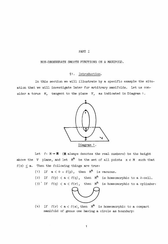
In this section we will illustrate by a specific example the situ-
ation that we will investigate later for arbitrary manifolds. Let us con-
sider a torus M, tangent to the plane V, as indicated in Diagram 1.
Diagram 1.
Let f: M -f R (R always denotes the real numbers) be the height
above the V plane, and let Ma be the set of all points x e M such that
f(x) < a. Then the following things are true:
(1) If a < 0 = f(p), then Ma is vacuous.
(2) If f(p) < a < f(q), then Ma is homeomorphic to a 2-cell.
(3)' If f(q) < a < f(r), then Ma is homeomorphic to a cylinder:
(4) If f(r) < a < f(s), then Ma is homeomorphic to a compact
manifold of genus one having a circle as boundary:
1
2 I. NON-DEGENERATE FUNCTIONS
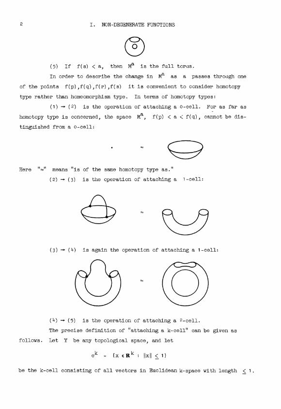
(5) If f(s) < a, then Ma' is the full torus.
In order to describe the change in Ma as a passes through one
of the points f(p),f(q),f(r),f(s) it is convenient to consider homotopy
type rather than homeomorphism type. In terms of homotopy types:
(1) is the operation of attaching a 0-cell. For as far as
homotopy type is concerned, the space Ma, f(p) < a < f(q), cannot be dis-
tinguished from a 0-cell:
Here means "is of the same homotopy type as."
(2) -* (3) is the operation of attaching a 1-cell:
(3) - (4) is again the operation of attaching a 1-cell:
(4) -. (5) is the operation of attaching a 2-cell.
The precise definition of "attaching a k-cell" can be given as
follows. Let Y be any topological space, and let
ek = {x ERk : 1xII < 1)
be the k-cell consisting of all vectors in Euclidean k-space with length < 1.

P. INTRODUCTION 3
The boundary
ek = (x E Rk IIxII =1)
will be denoted by Sk-1. If g:Sk-1 -+ Y is a continuous map then
Y .gek
(Y with a k-cell attached by g) is obtained by first taking the topologi-
cal sum (= disjoint union) of Y and ek, and then identifying each
x E Sk-1 with g(x) E Y. To tale care of the case k = 0 let eo be a
point and let 60 = S-1 be vacuous, so that Y with a 0-cell attached is
just the union of Y and a disjoint point.
As one might expect, the points p,q,r and s at which the homo-
topy type of Ma' changes, have a simple characterization in terms of f.
They are the critical points of the function. If we choose any coordinate
system (x,y) near these points, then the derivatives and y are(Tx
both zero. At p we can choose (x,y) so that f = x2 + y2, at s so
that f = constant -x2 - y2, and at q and r so that f = constant +
x y . Note that the number of minus signs in the expression for f at2 - 2
each point is the dimension of the cell we must attach to go from Ma to
Mb, where a < f(point) < b. Our first theorems will generalize these
facts for any differentiable function on a manifold.
REFERENCES
For further information on Morse Theory, the following sources are
extremely useful.
M. Morse, "The calculus of variations in the large," American
Mathematical Society, New York, 1934.
H. Seifert and W. Threlfall, "Variationsrechnung its Grossen,"
published in the United States by Chelsea, New York, 1951.
R. Bott, The stable homotopy of the classical groups, Annals of
Mathematics, Vol. 70 (1959), pp. 313-337.
R. Bott, Morse Theory and its application to homotopy theory,
Lecture notes by A. van de Ven (mimeographed), University of
Bonn, 1960.

4 I. NON-DEGENERATE FUNCTIONS
§2. Definitions and Lemmas.
The words "smooth" and "differentiable" will be used interchange-
ably to mean differentiable of class C". The tangent space of a smooth
manifold M at a point p will be denoted by TMp. If g: M -+ N is a
smooth map with g(p) = q, then the induced linear map of tangent spaces
will be denoted by g,: TMp TNq.
Now let f be a smooth real valued function on a manifold M. A
point p e M is called a critical point of f if the induced map
f*: TMp -T Rf(p) is zero. If we choose a local coordinate system
(x',...,xn) in a neighborhood U of p this means that
ofJ (P) _ ... = of
(p) = 0 .
ax axn
The real number f(p) is called a critical value of f.
We denote by Ma the set of all points x e M such that f(x) < a.
If a is not a critical value of f then it follows from the implicit
function theorem that Ma is a smooth manifold-with-boundary. The boundary
f- I(a) is a smooth submanifold of M.
A critical point p is called non-degenerate if and only if the
matrix
a2f(p))
axiaxj
is non-singular. It can be checked directly that non-degeneracy does not
depend on the coordinate system. This will follow also from the following
intrinsic definition.
If p is a critical point of f we define a symmetric bilinear
functional f** on TMp, called the Hessian of f at p. If v,w c TMp
then v and w have extensions v and w to vector fields. We let *
f**(v,w) = vp(w(f)), whereVP
is, of course, just v. We must show that
this is symmetric and well-defined. It is symmetric because
vp(w(f)) - wp(v(f)) _ [v,w]p(f) = 0
where [v,wl is the Poisson bracket of and w, and where [v,w] (f) = 0
Here w(f) denotes the directional derivative of f in the direction w.
§2. DEFINITIONS AND LEMMAS 5
since f has p as a critical point.
Therefore f** is symmetric. It is now clearly well-defined since
vp(w(f)) = v(w(f)) is independent of the extension v of v, while
(v(f)) is independent of w.wp
If (x1,...,xn) is a local coordinate system and v = E a.a
p,1 axi
w = E bj a-.Ip we can take w = E bj aj where bj now denotes a con-ax ax
stant function. Then
f**(v,w) = v(w(f))(p) = v(E b af) = Z a bf
(p)i axj i j i i ax
Iarespect to the basis ,...,
aX p axn p
We can now talk about the index and the nullity of the bilinear
functional ff* on TMp. The index of a bilinear functional H, on a vec-
tor space V, is defined to be the maximal dimension of a subspace of V
on which H is negative definite; the nullity is the dimension of the null-
space, i.e., the subspace consisting of all v E V such that H(v,w) = 0
for every w e V. The point p is obviously a non-degenerate critical
point of f if and only if f** on TMp has nullity equal to 0. The
index of f** on TMp will be referred to simply as the index of f at p.
The Lemma of Morse shows that the behaviour of f at p can be completely
described by this index. Before stating this lemma we first prove the
following:
LEMMA 2.1. Let f be a C°° function in a convex neigh-
borhood V of 0 in Rn, with f(o) = 0. Then
n
f(x1,...,xn) _ xigi(x1,...,xn)
i=t
for some suitable C" functions gi defined in V, with
gi(o) = )f (o).i
PROOF:
fdf(tx1,...,txn) 1 I of
f(xt,...,xn) = J dt = tx1,...,txn) xi dt
0 0 i=1i
1
Therefore we can let gi(x1...,xn) = f (tx1,...,txn) dt
0 i

6 I. NON-DEGENERATE FUNCTIONS
LEMMA 2.2 (Lemma of Morse). Let p be a non-degenerate
critical point for f. Then there is a local coordinate
system (y1,...,yn) in a neighborhood U of p with
yi(p) = 0 for all i and such that the identity
f - f(p) - (Y1)2- ... -(y% 2 + (yk+1)2
+ ... + (yn)2
holds throughout U, where is the index of f at p.
PROOF: We first show that if there is any such expression for f,
then X must be the index of f at p. For any coordinate system
(z1,...,zn), if
f(q) = f(p) - (z1(q))2- ... - (ZX(q))2 + (z11+1(9.))2 + ... + (Zn(q))2
then we have
-2 if i = j < x , ,
f (p) = 2 if i = J> Xaz1 azj
0 otherwise ,
which shows that the matrix representing f*,* with respect to the basis
a Ip,...,azn IP
is
Therefore there is a subspace of TMp of dimension l where f** is nega-
tive definite, and a subspace V of dimension n-X where f** is positive
definite. If there were a subspace of TMp of dimension greater than X
on which f** were negative definite then this subspace would intersect V,
which is clearly impossible. Therefore X is the index of f**.
We now show that a suitable coordinate system (y1,...,yn) exists.
Obviously we can assume that p is the origin of Rn and that f(p) = f(o) = 0.
By 2.1 we can write
f(x1,...,xn) _ xi gg(x1,...,xn)J= 1
for (x1,...,xn) in some neighborhood of 0. Since 0 is assumed to be a
critical point:
go (o) = a (0) = 0
§2. DEFINITIONS AND LEMMAS 7
Therefore, applying 2.1 to the gj we have
n
gj(x1)...,xn) _ xihij(x1) ...,xn)
i=1
for certain smooth functions hij. It follows that
n
f(x1) ...,xn) _ xixjhij(x1,...,xn)
i,j=1
We can assume that hij = hji, since we can write hij = '-2(hij+ hji),
and then have hij = Fiji and f = E xixjhij . Moreover the matrix (hij(o))
2
is equal to ( 2 (o)), and hence is non-singular.ax aX7
There is a non-singular transformation of the coordinate functions
which gives us the desired expression for f, in a perhaps smaller neigh-
borhood of 0. To see this we just imitate the usual diagonalization proof
for quadratic forms. (See for example, Birkhoff and MacLane, "A survey of
modern algebra," p. 271.) The key step can be described as follows.
Suppose by induction that there exist coordinates u1, ...,un in
a neighborhood U1 of 0 so that
f + (u1)2 + ... + (uY_1)2 + uiujHij(u1,...,un)
i,j>rthroughout U1; where the matrices (Hij(u1,...,un)) are symmetric. After
a linear change in the last n-r+1 coordinates we may assume that Hr,r(o) o.
Let g(u1,...,un) denote the square root of 1Hr,r(u1,...,un)I. This will
be a smooth, non-zero function of u1,...,un throughout some smaller neigh-
borhood U2 C U1 of 0. Now introduce new coordinates vl,...,vn by
vi=ui fori#r
vr(u1)...,un) = g(u1,...,un)[ur,+
uiHir(u1,...,un)/Hr,r,(u1,...sun)]'
i> r
It follows from the inverse function theorem that v1, ...,vn will serve as
coordinate functions within some sufficiently small neighborhood U3 of 0.
It is easily verified that f can be expressed as
f = + (vi)2 + vivjHij(v1,...,vn)
i<r i,j>r

8 I. NON-DEGENERATE FUNCTIONS
throughout U3. This completes the induction; and proves Lemma 2.2.
COROLLARY 2.3 Non-degenerate critical points are isolated.
Examples of degenerate critical points (for functions on R and
R2) are given below, together with pictures of their graphs.
(a) f(x) = x3. The origin (b) F(x) = e-1/X2 Sin2(,/X)
is a degenerate critical point. The origin is a degenerate, and
non-isolated, critical point.
(c) f(x,y) = x3 - 3xy2 = Real part of (x + iy)3.
(o.o) is a degenerate critical point (a "monkey saddle").

§2. DEFINITIONS AND LEMMAS 9
(d) f(x,y) = x2. The set of critical points, all of which
are degenerate, is the x axis, which is a sub-manifold of R 2.
(e) f(x,y) = x2y2. The set of critical points, all of which are
degenerate, consists of the union of the x and y axis, which is
not even a sub-manifold of R2.
We conclude this section with a discussion of 1-parameter groups of
diffeomorphisms. The reader is referred to K. Nomizu,"Lie Groups and Differ-
ential Geometry;'for more details.
A 1-parameter group of diffeomorphisms of a manifold M is a C00
map
W: R x M - M

10 I. NON-DEGENERATE FUNCTIONS
such that
1) for each t E R the map cpt: M -+ M defined by
cpt(q) = (p(t,q) is a diffeomorphism of M onto itself,
2) for all t,s c R we havept+s = Ipt ° ''s
Given a 1-parameter group cp of diffeomorphisms of M we define
a vector field X on M as follows. For every smooth real valued function
f let
lim f((Ph(q.)) - f(q)Xq(f) =h - o h
This vector field X is said to generate the group p.
LEMMA 2.4. A smooth vector field on M which vanishes
outside of a compact set K C M generates a unique 1-
parameter group of diffeomorphisms of M.
PROOF: Given any smooth curve
t - c(t) E M
it is convenient to define the velocity vector
c TMc(t)
by the identity (f) = hyme fc(t+hh-fc(t) (Compare §8.) Now let
be a 1-parameter group of diffeomorphisms, generated by the vector field X.
Then for each fixed q the curve
t -" pt(9)
satisfies the differential equation
dcpt(q)pct Xrot(q)
with initial condition cpe(q) = q. This is true since
dcpt(_q) (f)=
rlim Q f (Tt+h(q)) - f(cwt(9)) lim o f (roh(p) ) - f(p)X(f)h h p
where p = cpt(q). But it is well known that such a differential equation,
locally, has a unique solution which depends smoothly on the initial condi-
tion. (Compare Graves, "The Theory of Functions of Real Variables," p. 166.
Note that, in terms of local coordinates u1,...,un, the differential equa-i
tion takes on the more familiar form: dam- = x1(ul,...,un), i = 1,...,n.)

§2. DEFINITIONS AND LEMMAS 11
Thus for each point of M there exists a neighborhood U and a
number s > 0 so that the differential equation
dpt(q)- = Xcpt(q), CPO(q) = q
has a unique smooth solution for q e U, It! < e.
The compact set K can be covered by a finite number of such
neighborhoods U. Let e0 > 0 denote the smallest of the corresponding
numbers e. Setting pt(q) = q for q # K, it follows that this differen-
tial equation has a unique solution (pt(q) for It, <E0
and for all
q e M. This solution is smooth as a function of both variables. Further-
more, it is clear that cpt+s = Wt ° q>s providing that 1tj,1s1,1t+s1 < eo.
Therefore each such cpt is a diffeomorphism.
It only remains to define cpt for Iti > so. Any number t can
be expressed as a multiple of e0/2 plus a remainder r with Irk < eo/2
If t = k(so/2) + r with k > 0, set
Nt = 9PE0/2 ° CPEo/2 ° ... ° cpe0/2 ° 'Pr
where the transformation cpE /2 is iterated k times. If k < 0 it is0
only necessary to replace ke /2 by (p_E /2 iterated -k times. Thus (pt
0 0
is defined for all values of t. It is not difficult to verify that Tt is
well defined, smooth, and satisfies the condition (pt+s = Tt G (ps This
completes the proof of Lemma 2.4
REMARK: The hypothesis that X vanishes outside of a compact set
cannot be omitted. For example let M be the open unit interval (0,1) C R,
and let X be the standard vector field d on M. Then X does not_ff
generate any 1-parameter group of diffeomorphisms of M.
12 I. NON-DEGENERATE FUNCTIONS
§3. Homotopy Type in Terms of Critical Values.
Throughout this section, if f is a real valued function on a
manifold M, we let
Ma = f-1(- .,a] = (p e M : f(p) < a) .
THEOREM 3.1. Let f be a smooth real valued function
on a manifold M. Let a < b and suppose that the set
f-1[a,b], consisting of all p e M with a < f(p) < b,
is compact, and contains no critical points of f. Then
Ma is diffeomorphic to Mb. Furthermore, Ma is a de-
formation retract of Mb, so that the inclusion map
Ma Mb is a homotopy equivalence.
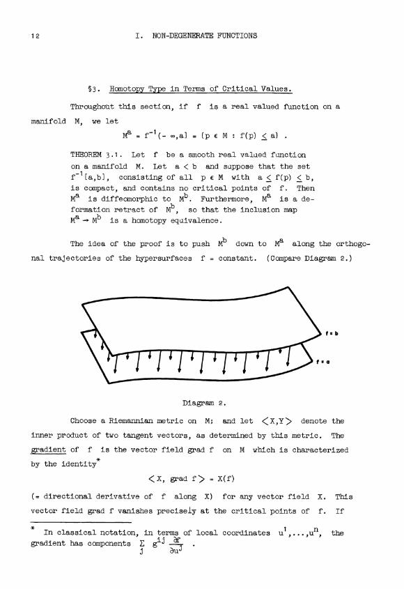
The idea of the proof is to push Mb down to Ma along the orthogo-
nal trajectories of the hypersurfaces f = constant. (Compare Diagram 2.)
Diagram 2.
Choose a Riemannian metric on M; and let < X,Y > denote the
inner product of two tangent vectors, as determined by this metric. The
gradient of f is the vector field grad f on M which is characterized
by the identity*
<X, grad f> = X(f)
(= directional derivative of f along X) for any vector field X. This
vector field grad f vanishes precisely at the critical points of f. If
* In classical notation, in terms of local coordinates u1,...,un, the
gradient has components E gij fj au3
§3. HOMOTOPY TYPE 13
c: R M is a curve with velocity vector'dE
note the identity
d grad f -d(dam
Let p: M -+ R be a smooth function which is equal to
1/ < grad f, grad f > throughout the compact set f-1[a,bl; and which vanishes
outside of a compact neighborhood of this set. Then the vector field X,
defined by
Xq = p(q) (grad f)q
satisfies the conditions of Lemma 2.4. Hence X generates a 1-parameter
group of diffeomorphisms
CPt: M - M.
For fixed q E M consider the function t f(cpt(q)). If Wt(q)
lies in the set f-1[a,bl, then
df(cpt(q)) dcpt(q)dt _ < d , grad f > = < X, grad f > = + 1 .
Thus the correspondence
t - f(Wt(q.))
is linear with derivative +1 as long as f(cpt(q)) lies between a and b.
Now consider the diffeomorphism cpb_a: M M. Clearly this carries
Ma diffeomorphically onto Mb. This proves the first half of 3.1.
Define a 1-parameter family of maps
rt: Mb . Mb
by
rt(q) = Jq if f(q) < a
''t(a-f(q))(q) if a < f(q) < b
Then re is the identity, and r1 is a retraction from Mb to ma. Hence
m' is a deformation retract of Mb. This completes the proof.
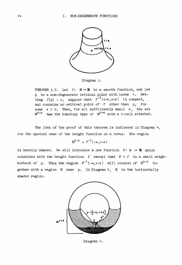
REMARK: The condition that f-1[a,b] is compact cannot be omitted.
For example Diagram 3 indicates a situation in which this set is not compact.
The manifold M does not contain the point p. Clearly Ma is not a de-
formation retract of Mb.
14 I. NON-DEGENERATE FUNCTIONS
Diagram 3.
THEOREM 3.2. Let f: M-+ R be a smooth function, and let
p be a non-degenerate critical point with index X. Set-
ting f(p) = c, suppose that f-1[c-e,c+el is compact,
and contains no critical point of f other then p, for
some s > 0. Then, for all sufficiently small e, the set
MC+e has the homotopy type ofMc-e
with a %-cell attached.
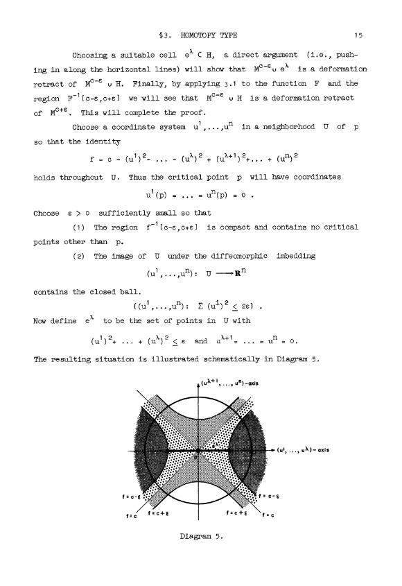
The idea of the proof of this theorem is indicated in Diagram 4,
for the special case of the height function on a torus. The region
Mc-e
= f-1(-co,c-e1
is heavily shaded. We will introduce a new function F: M -+ R which
coincides with the height function f except that F < f in a small neigh-
borhood of p. Thus the region F-1will consist of Mc-e to-
gether with a region H near p. In Diagram 4, H is the horizontally
shaded region.
MC+E
Diagram it.
§3. HOMOTOPY TYPE 15
Choosing a suitable cell e% C H, a direct argument (i.e., push-
ing in along the horizontal lines) will show that Mc-EU ex is a deformation
retract ofMc-E U H. Finally, by applying 3.1 to the function F and the
region F-1[c-E,c+E1 we will see thatMc-e u H is a deformation retract
ofMc+E. This will complete the proof.
Choose a coordinate system u1,.... un in a neighborhood U of p
so that the identity
f = c - (u1)2- ... - (uX)2 + (ut`+1)2+... + (un)2
holds throughout U. Thus the critical point p will have coordinates
u1(p) = ... = un(p) = 0 .
Choose e > 0 sufficiently small so that
(1) The region f-1[c-E,c+E1 is compact and contains no critical
points other than p.
(2) The image of U under the diffeomorphic imbedding
(u...... un): U --'Rn
contains the closed ball.
((u1,...,un): E (u')2 < 2E)
Now define eX to be the set of points in U with
1 ... X 2 X+1(u)2++ (u)< e and u= ... = un = 0.
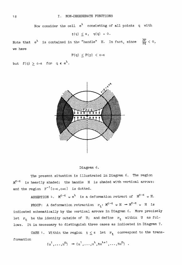
The resulting situation is illustrated schematically in Diagram 5.
Diagram 5.

16 I. NON-DEGENERATE FUNCTIONS
The coordinate lines represent the planes u11+1= ... = un = 0 and
u1 = ... = ux = 0 respectively; the circle represents the boundary of the
ball of radius; and the hyperbolas represent the hypersurfaces f-1(c-e)
and f-1(c+e). The regionM0-e
is heavily shaded; the region f-1[c-e,cl
is heavily dotted; and the region f-1[c,c+el is lightly dotted. The hori-
zontal dark line through p represents the cell e
Note that eX
nM°-e
is precisely the boundary ex, so that e
is attached to Mc-e as required. We must prove that Mc-eu eX is a de-
formation retract of Mc+e
Construct a new smooth function F: M -'f R as follows. Let
µ:R-pRbe a C" function satisfying the conditions
µ(o) > E
µ(r) 0 for r > 2e-1 < µ'(r) < 0 for all r,
where µ'(r) = dµ. Now let F coincide with f outside of the coordinate
neighborhood U, and let
F = f - µ((u1)2+. ..+(u2 + 2(uX+1 )2+...+2(un)2
within this coordinate neighborhood. It'is easily verified that F is a
well defined smooth function throughout M.
It is convenient to define two functions
t,11: U--i [0,oo)
by
_ (u1)2 + ... + (uX ) 2
{u?'+1) 2 + ... + (un) 2
Then f = c - t + q; so that:
for all q e U.
F(q) = c - (q) + q(q) - u(t(q) + 2q(q))
ASSERTION 1. The region F-1(-oo,c+el coincides with the region
Mc+e = f-1(- oo,c+el.
PROOF: Outside of the ellipsoid g + 2q < 2e the functions f and

U. HOMOTOPY TYPE 17
F coincide. Within this ellipsoid we have
F < f = c-g+q < c+ 2g+q < c+e
This completes the proof.
ASSERTION 2. The critical points of F are the same as those of f.
PROOF: Note that
Since
aFTq- 1 - 2µ'(g+2q) > 1 .
dF dg + dq
where the covectors dg and dq are simultaneously zero only at the origin,
it follows that F has no critical points in U other than the origin.
Now consider the region F-1[c-e,c+e]. By Assertion 1 together
with the inequality F < f we see that
F-1[C-e,C+e] C f-1[C-e,c+e]
Therefore this region is compact. It can contain no critical points of F
except possibly p. But
F(p) =c-µ(o) <c - e .
Hence F-1[c-e,c+e] contains no critical points. Together with 3.1 this
proves the following.
ASSERTION 3. The region F-1is a deformation retract ofMc+e
It will be convenient to denote this region F-1(-.,c-e] byMc-e
u H; where H denotes the closure of F-1(-co,c-El -Mc-e
REMARK: In the terminology of Smale, the region Mc-e v H is
described as Mc-e with a "handle" attached. It follows from Theorem 3.1
that the manifold-with-boundaryMC-e
U H is diffeomorphic to Mc+e This
fact is important in Smale's theory of differentiable manifolds. (Compare
S. Smale, Generalized Poincare's conjecture in dimensions greater than four,
Annals of Mathematics, Vol. 74 (1961), pp. 391-4o6.)
18 I. NON-DEGENERATE FUNCTIONS
Now consider the cell eX consisting of all points q with
t(q) < e, TI(q) = 0.
Note that eX is contained in the "handle" H. In fact, since < 0,
we have
F(q) < F(p) < c-e
but f(q) > c-e for q e ex.
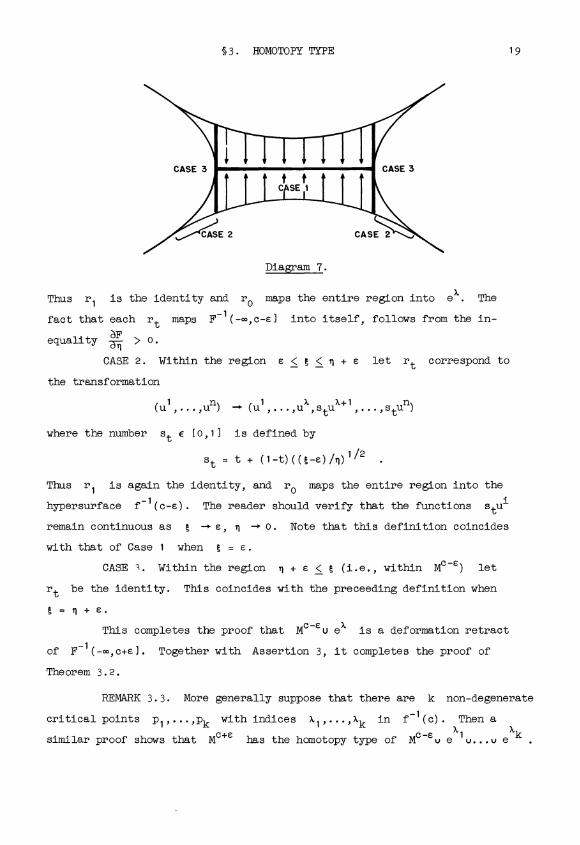
Diagram 6.
The present situation is illustrated in Diagram 6. The region
Mc-E is heavily shaded; the handle H is shaded with vertical arrows;
and the region F-1[c-e,c+e3 is dotted.
ASSERTION I+.Mc-e
u ex is a deformation retract ofMc-e
u H.
PROOF: A deformation retraction rt:Mc-e u H - Me-E
u H is
indicated schematically by the vertical arrows in Diagram 6. More precisely
let rt be the identity outside of U; and define rt within U as fol-
lows. It in necessary to distinguish three cases as indicated in Diagram 7.
CASE 1. Within the region g < e let rt correspond to the trans-
formation
(u1,...,un) _ (u1,...,ux,tu%+1,...,tun) .
§3. HOMOTOPY TYPE 19
CASE 2 CASE 2
Diagram 7.
Thus r1 is the identity and r0 maps the entire region into e The
fact that each rt maps F-1(-oo,c-el into itself, follows from the in-
equality > 0.Tq_
CASE 2. Within the region e < g < n + e let rt correspond to
the transformation
(u1,...Iun) -+ (ul,...,ux,stux+l,...,Stun)
where the number st e [0,11 is defined by
St = t + ( 1 -t) 1 /2
Thus r1 is again the identity, and r0 maps the entire region into the
hypersurface f-1(c-e). The reader should verify that the functions stu1
remain continuous as g -+ e, -' 0. Note that this definition coincides
with that of Case 1 when g = e.
CASE . Within the region q + e < g (i.e., within MC-e) let
rt be the identity. This coincides with the preceeding definition when
g = q + e.This completes the proof that MC-eu ex is a deformation retract
of F-1(-co,c+el. Together with Assertion 3, it completes the proof of
Theorem 3.2.
REMARK 3.3. More generally suppose that there are k non-degenerate
critical points pi,...,pk with indices x1,...,xk in f-1(c). Then ax x
similar proof shows that MC+e has the homotopy type of MC-eu a 1u...u e k
20 I. NON-DEGENERATE FUNCTIONS
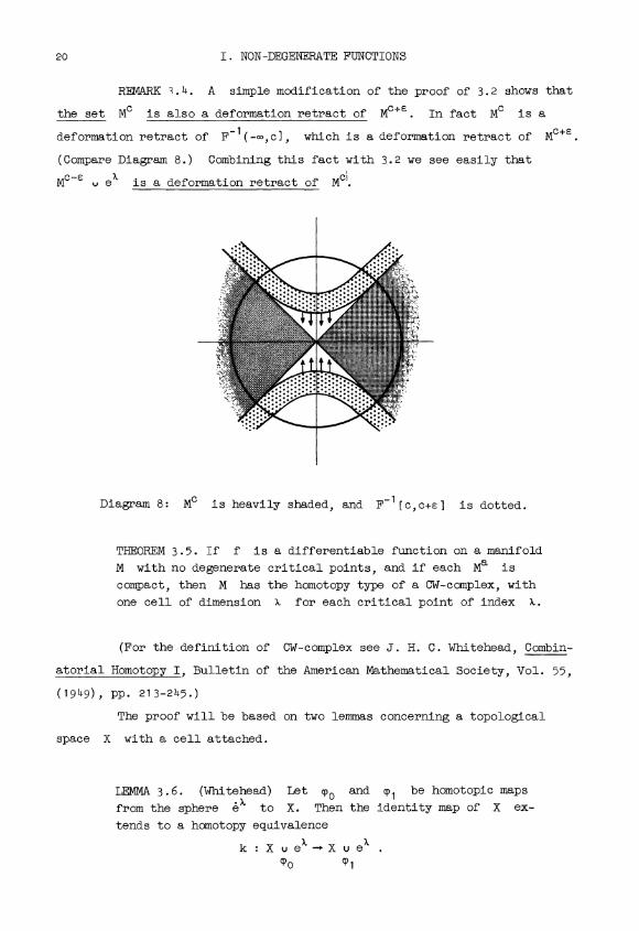
REMARK .4. A simple modification of the proof of 3.2 shows that
the set Mc is also a deformation retract of Mc+e. In fact Mc is a
deformation retract of F-1which is a deformation retract of Mc+e
(Compare Diagram 8.) Combining this fact with 3.2 we see easily thatMc-E
, et` is a deformation retract of MCI.
Diagram 8: Mc is heavily shaded, and F-1[c,c+e] is dotted.
THEOREM 3.5. If f is a differentiable function on a manifold
M with no degenerate critical points, and if each Ma is
compact, then M has the homotopy type of a CW-complex, with
one cell of dimension X for each critical point of index X.
(For the definition of CW-complex see J. H. C. Whitehead, Combin-
atorial Homotopy I, Bulletin of the American Mathematical Society, Vol. 55,
(1949), pp. 213-245.)
The proof will be based on two lemmas concerning a topological
space X with a cell attached.
LEMMA 3.6. (Whitehead) Let Woand cp1 be homotopic maps
from the sphere et' to X. Then the identity map of X ex-
tends to a homotopy equivalence
k:Xue%-*XueX'P0 CP 1

§3. HOMOTOPY TYPE 21
PROOF: Define k by the formulas
k(x) = x for x E X
k(tu) = 2tu for 0 < t < 2 u E
k(tu) = CP2_2t(u) for < t < 1, u E
Here 9t denotes the homotopy between Woand 91; and to denotes the
product of the scalar t with the unit vector u. A corresponding map
f: X u e -+ X u exW1 0
is defined by similar formulas. It is now not difficult to verify that the
compositions kF and fk are homotopic to the respective identity maps.
Thus k is a homotopy equivalence.
For further details the reader is referred to, Lemma 5 of J. H. C.
Whitehead, On Simply Connected 4-Dimensional Polyhedra, Commentarii Math.
Helvetici, Vol. 22 (1949), pp. 48-92.
LEMMA 3.7. Let W: e1''-+ X be an attaching map. Any
homotopy equivalence f: X -+ Y extends to a homotopy
equivalence
F : X uT eX -+ Y ..f(p eX.
PROOF: (Following an unpublished paper by P.Hilton.) Define F
by the conditions
FIX = f
Fled' = identity
Let g: Y -r X be a homotopy inverse to f and define
G: Y . efq) gfp
by the corresponding conditions GAY = g, identity.
Since gfp is homotopic to W, it follows from 3.6 that there is
a homotopy equivalence
k: X u e
gfp W
We will first prove that the composition
kGF: X u ex X u exW T
is homotopic to the identity map.
22 I. NON-DEGENERATE FUNCTIONS
Let ht be a homotopy between gf and the identity. Using the
specific definitions of k, G, and F, note that
kGF(x) = gf(x) for x E X,
kGF(tu) = 2tu for'O < t < 2 u e
11F(tu) h2-2t(P(u) for 2 < t < 1, u e
The required homotopy
qT: X sex X.e
is now defined by the formula
qT(x) = hT(x) for x e X ,
gT(tu) 1to for o < t < ,2T
, u
gT(tu) = h2-2t+TW(u) for 12< t < t, u e
Therefore F has a left homotopy inverse.
The proof that F is a homotopy equivalence will now be purely
formal, based on the following.
ASSERTION. If a map F has a left homotopy inverse L and a
right homotopy inverse R, then F is a homotopy equivalence; and
R (or L) is a 2-sided homotopy inverse.
PROOF: The relations
imply that
Consequently
LF ti identity, FR ti identity,
L-' L(FR) _ (LF)R ti R.
RF ti IF ti identity ,
which proves that R is a 2-sided inverse.
The proof of Lemma 3.7 can now be completed as follows. The rela-
tion
kGF ti identity
asserts that F has a left homotopy inverse; and a similar proof shows that
G has a left homotopy inverse.
Step 1. Since k(GF) identity, and k is known to have a left
inverse, it follows that (GF)k a identity.
§3. HOMOTOPY TYPE 23
Step 2. Since G(Fk) a identity, and G is known to have a left
inverse, it follows that (Fk)G ti identity.
Step 3. Since F(kG) a identity, and F has kG as left inverse
also, it follows that F is a homotopy equivalence. This completes the
proof of 3.7.
PROOF OF THEOREM 3.5. Let c1 < c2 < c3 < ... be the critical
values of f: M - R. The sequence (ci) has no cluster point since each
Ma is compact. The set Ma is vacuous for a < c1. Suppose
a c1,c21C31... and that Ma is of the homotopy type of a OW-complex.
Let c be the smallest ci > a. By Theorems 3.1, 3.2, and 3.3, Mc+e hasX %
the homotopy type of MC-cu e1 u...u e3(c) for certain maps q)1,.
T1 'J (c)
when e is small enough, and there is a homotopy equivalence h:Mc-e - Ma.
We have assumed that there is a homotopy equivalence h': Ma K, where K
is a OW-complex.
Then each h' o h o Tj is homotopic by cellular approximation to
a map
>Vj: 6 J -+ (), j-1) - skeleton of K.
Then K ue u...u ei(c) is a OW-complex, and has the same homotopy
`1 ''j (c)
type as Mc+e, by Lemmas 3.6, 3.7.
By induction it follows that each Ma' has the homotopy type of a
OW-complex. If M is compact this completes the proof. If M is not com-
pact, but all critical points lie in one of the compact sets Ma, then a
proof similar to that of Theorem 3.1 shows that the set Ma is a deformation
retract of M, so the proof is again complete.
If there are infinitely many critical points then the above con-
struction gives us an infinite sequence of homotopy equivalences
Mat C Ma2 C Ma3 C ...
f I f
K1 C K2 C K3 C ... ,
each extending the previous one. Let K denote the union of the Ki in the
direct limit topology, i.e., the finest possible compatible topology, and

24 I. NON-DEGENERATE FUNCTIONS
let g: M -r K be the limit map. Then g induces isomorphisms of homotopy
groups in all dimensions. We need only apply Theorem 1 of Combinatorial
homotopy I to conclude that g is a homotopy equivalence. [Whitehead's
theorem states that if M and K are both dominated by CW-complexes, then
any map M -+ K which induces isomorphisms of homotopy groups is a homotopy
equivalence. Certainly K is dominated by itself. To prove that M is
dominated by a CW-complex it is only necessary to consider M as a retract
of tubular neighborhood in some Euclidean space.] This completes the proof
of Theorem 3.5.
REMARK. We have also proved that each Ma has the homotopy type
of a finite CW-complex, with one cell of dimension X for each critical
point of index X in Ma. This is true even if a is a critical value.
(Compare Remark 3.4.)

§4. EXAMPLES 25
§4. Examples.
As an application of the theorems of §3 we shall prove:
THEOREM 4.1 (Reeb). If M is a compact manifold and f
is a differentiable function on M with only two critical
points, both of which are non-degenerate, then M is
homeomorphic to a sphere.
PROOF: This follows from Theorem 3.1 together with the Lemma of
Morse (§2.2). The two critical points must be the minimum and maximum
points. Say that f(p) = 0 is the mimimum and f(q) = 1 is the maximum.
If s is small enough then the sets Ms = f_1[0,e) and f_1[1-e,11 are
closed n-cells by §2.2. But Me is homeomorphic to M1-E by §3.1. Thus
M is the union of two closed n-cells, M1-E and f-1[1-e,1), matched
along their common boundary. It is now easy to construct a homeomorphism
between M and Sn.
REMARK 1. The theorem remains true even if the critical points are
degenerate. However, the proof is more difficult. (Compare Milnor, Differ-
ential topology, in "Lectures on Modern Mathematics II," ed. by T. L:.Saaty
(Wiley, 1964), pp. 165-183; Theorem 1'; or R. Rosen, A weak form of the
star conjecture for manifolds, Abstract 570-28, Notices Amer. Math Soc.,
Vol. 7 (1960), p. 380; Lemma 1.)
REMARK 2. It is not true that M must be diffeomorphic to Sn with
its usual differentiable structure.(Compare: Milnor, On manifolds homeomor-
phic to the 7-sphere, Annals of Mathematics, Vol. 64 (1956), pp. 399-405.
In this paper a 7-sphere with a non-standard differentiable structure is
proved to be topologically S7 by finding a function on it with two non-
26 I. NON-DEGENERATE FUNCTIONS
degenerate critical points.)
As another application of the previous theorems we note that if an
n-manifold has a non-degenerate function on it with only three critical
points then they have index 0, n and n/2 (by Poincare duality), and the
manifold has the homotopy type of an n/2-sphere with an n-cell attached.
See J. Eells and N. Kuiper, Manifolds which are like projective planes,
Inst. des Hautes Etudes Sci., Publ. Math. 14, 1962. Such a function exists
for example on the real or complex projective plane.
Let CPn be complex projective n-space. We will think of CPn as
equivalence classes of (n+1)-tuples (z0,...,zn) of complex numbers, with
EIzj12 = 1. Denote the equivalence class of (z0,...,zn) by (z0:z1:...:zn).
Define a real valued function f on CPn by the identity
f(z0:z1:...:zn) = I cj1zjl2
where c0,c1,...,cn are distinct real constants.
In order to determine the critical points of f, consider the
following local coordinate system. Let U0 be the set of (zo:z1:...:zn)
with z0 0, and setI Za I
zo= x+ iyjZj
Then
x1,y1,...,xn,yn: U0 - R
are the required coordinate functions, mapping U0 diffeomorphically onto
the open unit ball in R 2ri. Clearly
zjI2 = xj2 + yj2Izol2
= 1 - E (xj2 + yj2)
so that
f = c0j=1
throughout the coordinate neighborhood U0. Thus the only critical point of
f within U. lies at the center point
p0 = (1:0:0:...:0)
of the coordinate system. At this point f is non-degenerate; and has
index equal to twice the number of j with cj < co,
Similarly one can consider other coordinate systems centered at the
points
p1 = (0:1:0: ...:0),...,Pn = (0:0:...:0:1)
§4. EXAMPLES 27
It follows that p0,pi,...,pn are the only critical points of f. The
index of f at pk is equal to twice the number of j with cj < ck.
Thus every possible even index between 0 and 2n occurs exactly once.
By Theorem 3.5:
C Pn has the homotopy type of a CW-complex of the form
e° u e2 u e4 u...u e2n
It follows that the integral homology groups of CPn are given by
Fii(CPn;Z) Z for i = 0,2,4,...,2n
l 0 for other values of i
28 I. NON-DEGENERATE FUNCTIONS
§5. The Morse Inequalities.
In Morse's original treatment of this subject, Theorem 3.5 was not
available. The relationship between the topology of M and the critical
points of a real valued function on M were described instead in terms of
a collection of inequalities. This section will describe this original
point of view.
DEFINITION: Let S be a function from certain pairs of spaces to
the integers. S is subadditive if whenever XD Y: )Z we have S(X,Z) <
S(X,Y) + S(Y,Z). If equality holds, S is called additive.
As an example, given any field F as coefficient group, let
RX(X,Y) = Xth Betti number of (X,Y)
= rank over F of HX(X,Y;F)
for any pair (X,Y) such that this rank is finite. RX is subadditive, as
is easily seen by examining the following portion of the exact sequence for
(X,Y,Z):
... -+ HX(Y,Z) HX(X,Z) - HX(X,Y) -+ ...
The Euler characteristic X(X,Y) is additive, where X(X,Y) _
E (-1)X RX(X,Y).
LEMMA 5.1. Let S be subadditive and let X0C...C Xn.
Then S(Xn,XO)< S(Xi,Xi_,). If S is additive then
equality holds. 1
PROOF: Induction on n. For n = 1, equality holds trivially and
the case n = 2 is the definition of [sub] additivity.n-1
If the result is true for n - 1, then S(Xn_1,XO) < S(Xi,Xi_1).
}Therefore S(Xn,X0) < S(Xn_1,Xa) + S(Xn,Xn_1) < 2; S(Xi,X1_1) and the result
1
is true for n.
Let S(X,o) = S(X). Taking X. = 0 in Lemma 5.1, we have
n
(1) S(Xn) <S(Xi,Xi-1)
with equality if S is additive.
§5. THE MORSE INEQUALITIES 29
Let M be a compact manifold and f a differentiable function
on M with isolated, non-degenerate, critical points. Let a1 <...< ak
be such that Mai contains exactly i critical points, and Mak = M.
Then
H*(Mat Mat-1) = H (Mai-1 e% 1 Mai-1)
where is the index of the
critical point,.X. ),
H*(e 1,e 1) by excision,
coefficient group in dimension Xi
0 otherwise.
Applying (1) to 0 = Mo C...C M k = M with S = R. we havea a
kR),(Ma1,Ma1-1)
= CX;
i=1
where C. denotes the number of critical points of index X. Applying this
formula to the case S = X we have
k
x(M) = X(Ma1,Ma1-1) = C0 - C1 + C2 -+...+ Cn
i=1
Thus we have proven:
argument.
THEOREM 5.2 (Weak Morse Inequalities). If Cx denotes the
number of critical points of index X on the compact mani-
fold M then
RX(M) < CX , and
E (-1)" RX(M) (-1)X CX
Slightly sharper inequalities can be proven by the following
LEMMA 5.3. The function S. is subadditive, where
SX(X,Y) = RX(X,Y) - Rx_1(X,Y) + Rx_2(X,Y) - +...+ R0(X,Y)
PROOF: Given an exact sequence
h+A' B Ck... ...-+D-+0of vector spaces note that the rank of the homomorphism h plus the rank
of i is equal to the rank of A. Therefore,
30 I. NON-DEGENERATE FUNCTIONS
rank h = rank A - rank i
= rank A - rank B + rank j
= rank A - rank B + rank C - rank k
= rank A - rank B + rank C - +...+ rank D .
Hence the last expression is > 0. Now consider the homology exact sequence
of a triple X J Y J Z. Applying this computation to the homomorphism
Hx+1 (X,Y)a
H,,(Y,Z)
we see that
rank 3 = RX(Y,Z) - RX(X,Z) + RX(X,Y) - Rx_1(Y,Z) + ... > o
Collecting terms, this means that
S,(Y,Z) - S (X,Z) + SX(X,Y) > o
which completes the proof.
Applying this subadditive function S1, to the spaces
0 C Mat C Mat C...C Mak
we obtain the Morse inequalities:
or
Sx(M) <
k
a aX(Mi'Mi-1) = CX - CX-1 +-...+ Co
i=1
(40 R>(M) - RX_1(M) +-...+ Ro(M) < CX - CX_1+ -...+ Co.
These inequalities are definitely sharper than the previous ones.
In fact, adding (4x) and (4,_1), one obtains (2x); and comparing (40
with (4,_1) for x> n one obtains the equality (3).
As an illustration of the use of the Morse inequalities, suppose
that C,+1 = 0. Then R,+1 must also be zero. Comparing the inequalities
(4.) and (41,+1), we see that
RX - R)6_1 +-...+ Ro = C% - C1'_1 -...± Co .
Now suppose that C.-1 is also zero. Then R._1 = 0, and a similar argu-
ment shows that
Rx-2 - Rx-3 +-...± Ro = Cx-2-Cx-3 +-...± Co .

§5. THE MORSE INEQUALITIES
Subtracting this from the equality above we obtain the following:
COROLLARY 5.4. If Cx+1 = CX_1 = 0 then R. = C. and
R)L+1 = RX_1 = 0.
31
(Of course this would also follow from Theorem 3.5.) Note that
this corollary enables us to find the homology groups of complex projective
space (see §4) without making use of Theorem 3.5.

32 I. NON-DEGENERATE FUNCTIONS
§6. Manifolds in Euclidean Space.
Although we have so far considered, on a manifold, only functions
which have no degenerate critical points, we have not yet even shown that
such functions always exist. In this section we will construct many func-
tions with no degenerate critical points, on any manifold embedded in Rn.
In fact, if for fixed p c Rn define the function LP: M - R by LL(q) _
lip-gII2. It will turn out that for almost all p, the function Lp has
only non-degenerate critical points.
Let M C Rn be a manifold of dimension k < n, differentiably em-
bedded in Rn. Let N C M x Rn be defined by
N = ((q,v): q e M, v perpendicular to M at q).
It is not difficult to show that N is an n-dimensional manifold
differentiably embedded in R2ri. (N is the total space of the normal
vector bundle of M.)
Let E: N -+ Rn be E(q,v) = q + v. (E is the "endpoint" map.)
E(4,v)
DEFINITION. e E Rn is a focal point of (M,q) with multiplicity
µ if e = q + v where (q,v) E N and the Jacobian of E at (q,v) has
nullity µ > 0. The point e will be called a focal point of M if e is
a focal point of (M,q) for some q e M.
Intuitively, a focal point of M is a point in Rn where nearby
normals intersect.
We will use the following theorem, which we will not prove.
§6. MANIFOLDS IN EUCLIDEAN SPACE 33
THEOREM 6.1 (Sard). If M1 and M2 are differentiable
manifolds having a countable basis, of the same dimension,
and f: M1 M2 is of class C1, then the image of the
set of critical points has measure 0 in M2-
A critical point of f is a point where the Jacobian of f is
singular. For a proof see de Rham, "Variotes Differentiables," Hermann,
Paris, 1955, p. 10.
COROLLARY 6.2. For almost all x e Rn, the point x is
not a focal point of M.
PROOF: We have just seen that N is an n-manifold. The point x
is a focal point iff x is in the image of the set of critical points of
E: N -s Rn. Therefore the set of focal points has measure 0.
For a better understanding of the concept of focal point, it is con-
venient to introduce the "second fundamental form" of a manifold in Euclidean
space. We will not attempt to give an invariant definition; but will make
use of a fixed local coordinate system.
Let u1,...,uk be coordinates for a region of the manifold M C R.
Then the inclusion map from M to Rn determines n smooth functions
1 k 1 kx1(u ,...,u ),...,xn(u '...,u)
These functions will be written briefly as x(u1,...,uk) where x =
(x1,...,xn). To be consistent the point q e M C Rn will now be denoted by
q.
The first fundamental form associated with the coordinate system is
defined to be the symmetric matrix of real valued functions
(gij) _ (3ui - j) .
The second fundamental form on the other hand, is a symmetric matrix (ij)
of vector valued functions.2-'
It is defined as follows. The vector a- at a point of M canu aukk
be expressed as the sum of a vector tangent to M and a vector normal to M.2-
Define T.. to be the normal component ofau
x . Given any unit vectorau
v which is normal to M at q the matrix
(v ) _ (v i.auJ 1j

34 I. NON-DEGENERATE FUNCTIONS
can be called the "second fundamental form of M at q in the direction
v."
It will simplify the discussion to assume that the coordinates
have been chosen to that gi3, evaluated at q, is the identity matrix.
Then the eigenvalues of the matrix ( v are called the principal
curvatures K1,...,KK of M at -1 in the normal direction v. The re-
ciprocals of these principal curvatures are called the princi-
)pal radii of curvature. Of course it may happen that the matrix (v .7ii
is singular. In this case one or more of the Ki will be zero; and hence
the corresponding radii Kit will not be defined.
Now consider the normal line 2 consisting of all q + tv, where
v is a fixed unit vector orthogonal to M at q
LEMMA 6.3. The focal points of (M q) along f are pre-
cisely the points _q -1 _V,q+ Ki v where 1 < i< k, Ki / o.
Thus there are at most, k focal points of (M,q) along
f, each being counted with its proper multiplicity.
1 k 1 kPROOF: Choose n-k vector fields w1(u ,...,u ),...,wn_k(u ,...,u )
along the manifold so that w1,...;wn_k are unit vectors which are orthogo-
nal to each other and to M. We can introduce coordinates (u1,...,uk,
t1,...Itn-k) on the manifold N C M x e as follows. Let (u1,...,uk,t1,..
to-k) correspond to the pointn-k
\(x(u1,...,uk), to wa(u1,...,uk)1 e N
a=1
Then the function
E : N -. Rn
gives rise to the correspondence
1 k 1 n-k e' 1 k a -+ 1 k(ll ,...,U ,t ,...,t ) X(u ,...,u ) +J t wa(u ,...,u ) ,
with partial derivatives
aB aX + to awa
aul au1 aul
aea a
Taking the inner products of these n-vectors with the linearly independent
§6. MANIFOLDS IN EUCLIDEAN SPACE
vectors axl, axk, w1'...;wn_k we will obtain an nxn matrix whoseau au
rank equals the rank of the Jacobian of E at the corresponding point.
This nxn matrix clearly has the following form
yax aX +
toawa
ax \1 to awa w 1 1au auj aul 0 / (
a TIT S
0 identity
matrix
35
Thus the nullity is equal to the nullity of the upper left hand block. Using
the identity
o=7'T
( W ax=
aWa ax + W x1
aauk au1 auk
a2)u1auj
we see that this upper left hand block is just the matrix
-.( gig ta wa Iiia
Thus:
ASSERTION 6.4. q + tv is a focal point of (M,q) with multiplicity
µ if and only if the matrix
(*) (gig - tv Iii )is singular, with nullity P.
Now suppose that (gij) is the identity matrix. Then (*) is singu-
lar if and only if -f is an eigenvalue of the matrix (v ) Further-
more the multiplicity µ is equal to the multiplicity of - as eigenvalue.
This completes the proof of Lemma 6.3.
Now for fixed p E Rn let us study the function
Ip = f : M - Rwhere
f(x(u1,...,uk)) = Ij-X(u1,...,uk) - pII2 = x x - 2x p + p p .
We have
of = 2 ax(x - p)
aul TIT
Thus f has a critical point at q if and only if q - p is normal to M
at q

36 I. NON-DEGENERATE FUNCTIONS
The second partial derivatives at a critical point are given by
2f_= 2( ax , ax
+x
. lX
au au aul auk a 3
Setting p = x + tv, as in the proof of Lemma 6.3, this becomes
2(gi. - tvau auk
Therefore:
LEMMA 6.5. The point q e M is a degenerate critical point
of f = L5- if and only if p is a focal point of (M,q).
The nullity of q as critical point is equal to the multi-
plicity of p as focal point.
Combining this result with Corollary 6.2 to Sari's theorem, we
immediately obtain:
THEOREM 6.6. For almost all p e Rn (all but a set ofmeasure 0) the function
LL: M -+R
has no degenerate critical points.
This theorem has several interesting consequences.
COROLLARY 6.7. On any manifold M there exists a dif-
ferentiable function, with no degenerate critical points,
for which each Ma is compact.
PROOF: This follows from Theorem 6.6 and the fact that an n-dimen-
sional manifold M can be embedded differentiably as.a closed subset of
R2n+1(see Whitney, Geometric Integration Theory, p. 113).
APPLICATION 1. A differentiable manifold has the homotopy type of
a CW-complex. This follows from the above corollary and Theorem 3.5.
APPLICATION 2. On a compact manifold M there is a vector field
X such that the sum of the indices of the critical points of X equals
x(M), the Euler characteristic of M. This can be seen as follows: for
any differentiable function f on M we have x(M) = E (-1)x Cx where C.
is the number of critical points with index X. But (-1)x is the index of
the vector field grad f at a point where f has index x.
§6. MANIFOLDS IN EUCLIDEAN SPACE 37
It follows that the sum of the indices of any vector field on M
is equal to x(M) because this sum is a topological invariant (see Steen-
rod, "The Topology of Fibre Bundles," §39.7).
The preceding corollary can be sharpened as follows. Let k > 0
be an integer and let K C M be a compact set.
COROLLARY 6.8. Any bounded smooth function f: M -+ R can
be uniformly approximated by a smooth function g which
has no degenerate critical points. Furthermore g can be
chosen so that the i-th derivatives of g on the compact
set K uniformly approximate the corresponding derivatives
of f, for i < k.
(Compare M. Morse, The critical points of a function of n vari-
ables, Transactions of the American Mathematical Society, Vol. 33 (1931),
pp. 71-91.)
PROOF: Choose some imbedding h: M -+ Rn of M as a bounded sub-
set of some euclidean space so that the first coordinate h1 is precisely
the given function f. Let c be a large number. Choose a point
p = (-C+e1,e2,..., En)
close to (-C,0,...,o) E Rn so that the function LP: M -+ R is non-
degenerate; and set(x) - C2
g(x) 2C
Clearly g is non-degenerate. A short computation shows that
g(x) = f(x) + I hi(x)2/2c - eihi(x)/c + ei2/2c
1 1 1
Clearly, if c is large and the ei are small, then g will approximate
f as required.
The above theory can also be used to describe the index of the
function
at a critical point.
LEMMA 6.9. (Index theorem for Lp.) The index of Lp
at a non-degenerate critical point q e M is equal to
the number of focal points of (M,q) which lie on the
segment from q to p; each focal point being counted
with its multiplicity.

38 I. NON-DEGENERATE FUNCTIONS
An analogous statement in Part III (the Morse Index Theorem) will
be of fundamental importance.
PROOF: The index of the matrix
a2
2(gij - tv ij)au au
is equal to the number of negative eigenvalues. Assuming that (gij) is
the identity matrix, this is equal to the number of eigenvalues of (v lid)
which are >
7. Comparing this statement with 6.3, the conclusion follows.
§7. THE LEFSCHETZ THEOREM 39
§7. The Lefschetz Theorem on Hyperplane Sections.
As an application of the ideas which have been developed, we will
prove some results concerning the topology of algebraic varieties. These
were originally proved by Lefschetz, using quite different arguments. The
present version is due to Andreotti and Frankel*.
THEOREM 7.1. If M C Cn is a non-singular affine alge-
braic variety in complex n-space with real dimension 2k,
then
Hi(M;Z) = 0 for i > k.
This is a consequence of the stronger:
THEOREM 7.2. A complex analytic manifold M of complex
dimension k, bianalytically embedded as a closed subset
of Cn has the homotopy type of a k-dimensional CW-complex.
The proof will be broken up into several steps. First consider a
quadratic form in k complex variables
Q(z1,...,zk) = Ibhj
zhzi .
If we substitute xh + iyh for zh, and then take the real part of Q we
obtain a real quadratic form in 2k real variables:
Q'(x1,...,xk,yt,...,yk) = real part of bhj(xh+iyh)(x3+iy3)
ASSERTION 1. If e is an eigenvalue of Q' with multiplicity µ,
then -e is also an eigenvalue with the same multiplicity µ.
PROOF. The identity Q(iz1,...,izk) = -Q(z1,...,zk) shows that
the quadratic form Q' can be transformed into -Q' by an orthogonal
change of variables. Assertion 1 clearly follows.
11
See S. Lefschetz, "L'analysis situs et la geometrie algebrique," Paris,
1921+; and A. Andreotti and T. Frankel, The Lefschetz theorem on hyperplane
sections, Annals of Mathematics, Vol. 69 (1959), pp. 713-717.

4o I. NON-DEGENERATE FUNCTIONS
Now consider a complex manifold M which is bianalytically imbed-
ded as a subset of Cn. Let q be a point of M.
ASSERTION 2. The focal points of (M,q) along any normal line 2
occur in pairs which are situated symmetrically about q.
In other words if q + tv is a focal point, then q - tv is a
focal point with the same multiplicity.
PROOF. Choose complex coordinates z1,...,zk for M in a neigh-
borhood of q so that z1(q) = ... = zk(q) = 0. The inclusion map M-+ Cn
determines n complex analytic functions
WC, wa(z1 ,...,zk ), a = 1, ..,n.
Let v be a fixed unit vector which is orthogonal to M at q. Consider
the Hermitian inner product
wava = wa(z1,...,zk)va
of w and v. This can be expanded as a complex power series
I wa(z1,...,zk)va = constant + Q(z1,...,zk) + higher terms,
where Q denotes a homogeneous quadratic function. (The linear terms van-
ish since v is orthogonal to M.)
Now substitute xh + iyh for zh so as to obtain a real coordinate
system for M; and consider the real inner product
w v = real part of wava .
This function has the real power series expansion
w- v = constant + Q1(x1 xk 1 k,Y higher terms.
Clearly the quadratic terms Q' determine the second fundamental form of
M at q in the normal direction v. By Assertion 1 the eigenvalues of
Q' occur in equal and opposite pairs. Hence the focal points of (M,q)
along the line through q and q + v also occur in symmetric pairs. This
proves Assertion 2.
We are now ready to prove 7.2. Choose a point p e Cn so that the
squared-distance function
§7. THE LEFSCHETZ THEOREM 41
Y M -+ R
has no degenerate critical points. Since M is a closed subset of Cn, it
is clear that each set
Ma =
is compact. Now consider the index of Lp at a critical point q. Accord-
ing to 6.9, this index is equal to the number of focal points of (M,q)
which lie on the line segment from p to q. But there are at most 2k
focal points along the full line through p and q; and these are distri-
buted symmetrically about q. Hence at most k of them can lie between p
and q.
Thus the index of Lp at q is < k. It follows that M has the
homotopy type of a OW-complex of dimension < k; which completes the proof
of 7.2.
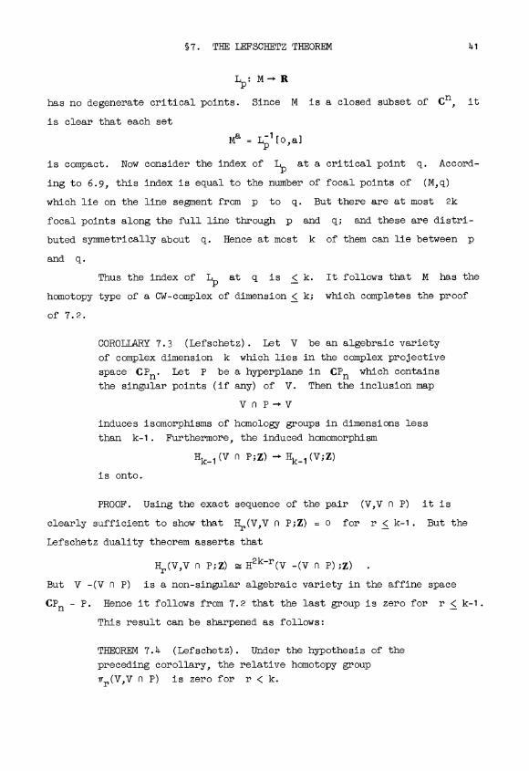
COROLLARY 7.3 (Lefschetz). Let V be an algebraic variety
of complex dimension k which lies in the complex projective
space CPn. Let P be a hyperplane in CPn which contains
the singular points (if any) of V. Then the inclusion map
V n P-Vinduces isomorphisms of homology groups in dimensions less
than k-1. Furthermore, the induced homomorphism
Hk_1(V n P;Z) Hk-l(V;Z)
is onto.
PROOF. Using the exact sequence of the pair (V,V n P) it is
clearly sufficient to show that H1,(V,V n P;Z) = 0 for r < k-1. But the
Lefschetz duality theorem asserts that
Hr,(V,V n P;Z) = H2k-r(V -(V n P) ;Z)
But V -(V n P) is a non-singular algebraic variety in the affine space
CPn - P. Hence it follows from 7.2 that the last group is zero for r < k-1.
This result can be sharpened as follows:
THEOREM 7.4 (Lefschetz). Under the hypothesis of the
preceding corollary, the relative homotopy group
Trr(V,V n P) is zero for r < k.
42 I. NON-DEGENERATE FUNCTIONS
PROOF. The proof will be based on the hypothesis that some neigh-
borhood U of V n P can be deformed into V n P within V. This can be
proved, for example, using the theorem that algebraic varieties can be tri-
angulated.
In place of the function LP: V - V n P -+ R we will use f: V -+ R
where
f(x)ro for x e V n P
t/Lp(x) for x j P.
Since the critical points of Lp have index < k it follows that
the critical points of f have index > 2k - k = k. The function f has
no degenerate critical points with s < f < co. Therefore V has the
homotopy type of Ve = f-1[o,e] with finitely many cells of dimension > k
attached.
Choose e small enough so that VE C U. Let Ir denote the unit
r-cube. Then every map of the pair (Ir,Ir) into (V,V n P) can be deform-
ed into a map
(Ir,Ir) - (V-,V n P) C (U,V n P) ,
since r < k, and hence can be deformed into V n P. This completes the
proof.

PART II
A RAPID COURSE IN RIEMANNIAN GEOMETRY
§8. Covariant Differentiation
The object of Part II will be to give a rapid outline of some basic
concepts of Riemannian geometry which will be needed later. For more infor-
mation the reader should consult Nomizu, "Lie groups and differential geo-
metry. Math. Soc. Japan, 1956; Helgason, "Differential geometry and sym-
metric spaces," Academic Press, 1962; Sternberg, "Lectures on differential
geometry," Prentice-Hall, 1964; or Laugwitz, "Differential and Riemannian
geometry," Academic Press, 1965.
Let M be a smooth manifold.
DEFINITION. An affine connection at a point p E M is a function
which assigns to each tangent vector Xp E TMp and to each vector field Y
a new tangent vector
Xp - Y E TMp
called the covariant derivative of Y in the direction Xp. This is re-
quired to be bilinear as a function of Xp and Y. Furthermore, if
f: M- Ris a real valued function, and if fY denotes the vector field
(fY)q = f(q)Yq
'then h is required to satisfy the identity
Xp I- (fY) = (Xpf)Yp + f(p)Xp I- Y .
Note that our X F Y coincides with Nomizu's Vxy. The notation is in-
tended to suggest that the differential operator X acts on the vector field
Y.
44 II. RIEMANNIAN GEOMETRY
(As usual, Xpf denotes the directional derivative of f in the direction
XP.)
A global affine connection (or briefly a connection) on M is a
function which assigns to each p e M an affine connection Fp at p,
satisfying the following smoothness condition.
1) If X and Y are smooth vector fields on M then the vector
field X F Y, defined by the identity
(X FY)p=Xp FpY ,
must also be smooth.
Note that:
(2) X F Y is bilinear as a function of X and Y
(3) (fX) F Y = f(X F Y) ,
(4) (X F (fY) = (Xf)Y + f(X F Y)
Conditions (1), (2), (3), (4) can be taken as the definition of
a connection.
In terms of local coordinates ul,...,un defined on a coordinate
neighborhood U C M, the connection F is determined by n3 smooth real
valued functions ik on U, as follows. Let ak denote the vector
field on U. Then any vector field X on U can be expressedau
uniquely as
X = k xkakk=1
where the xk are real valued functions on U. In particular the vector
field ai F ai can be expressed as
(5) ai F a _rij k
These functions i, determine the connection completely on U.
In fact given vector fields X = x'ai and Y = yJaj one can
expand X F Y by the rules (2), (3), (4); yielding the formula
(6) X F Y = xiyki)akk i

§8. COVARIANT DIFFERENTIATION 45
where the symbol yki stands for the real valued function
y'i = aiyk + ij yj
Conversely, given any smooth real valued functions ik on U,
one can define X F Y by the formula (6). The result clearly satisfies
the conditions (1), (2), (3), (4), (5).
Using the connection F one can define the covariant derivative of
a vector field along a curve in M. First some definitions.
A parametrized curve in M is a smooth function c from the real
numbers to M. A vector field V along the curve c is a function which
assigns to each t e R a tangent vector
Vt E TMc(t)
This is required to be smooth in the following sense: For any smooth func-
tion f on M the correspondence
t Vtf
should define a smooth function on R.
As an example the velocity vector field of the curve is the(ifvector field along c which is defined by the rule
do dUE -
c* T£
HereTdt
denotes the standard vector field on the real numbers, and
c*: TRt TMc(t)
denotes the homomorphism of tangent spaces induced by the map c. (Compare
Diagram 9.)de
Diagram 9
46 II. RIEMANNIAN GEOMETRY
Now suppose that M is provided with an affine connection. Then
any vector field V along c determines a new vector field DV along c
called the covariant derivative of V. The operation
V DVffu
is characterized by the following three axioms.
a) D(V+W)= ur+-Tf-
D(fV) _ V + f DV.
c) If V is induced by a vector field Y on M, that is if
VtYc(t)
for each t, then DV is equal to F Y_CTE
(= the covariant derivative of Y in the direction of the
velocity vector of c)
LEMMA 8.1. There is one and only one operation V -+ DV
which satisfies these three conditions.
PROOF: Choose a local coordinate system for M, and let
u1(t),. .,un(t) denote the coordinates of the point c(t). The vector
field V can be expressed uniquely in the form
V = I v4j
where v1,...,vn are real valued functions on R (or an appropriate open
subset of R), and a1,...1an are the standard vector fields on the co-
ordinate neighborhood. It follows from (a), (b), and (c) that
i
dam- + = ri vi, ak3
k i,j
Conversely, defining DV by this formula, it is not difficult to verify
that conditions (a), (b), and (c) are satisfied.
A vector field V along c is said to be a parallel vector field
if the covariant derivative is identically zero.CT:E
§8. COVARIANT DIFFERENTIATION
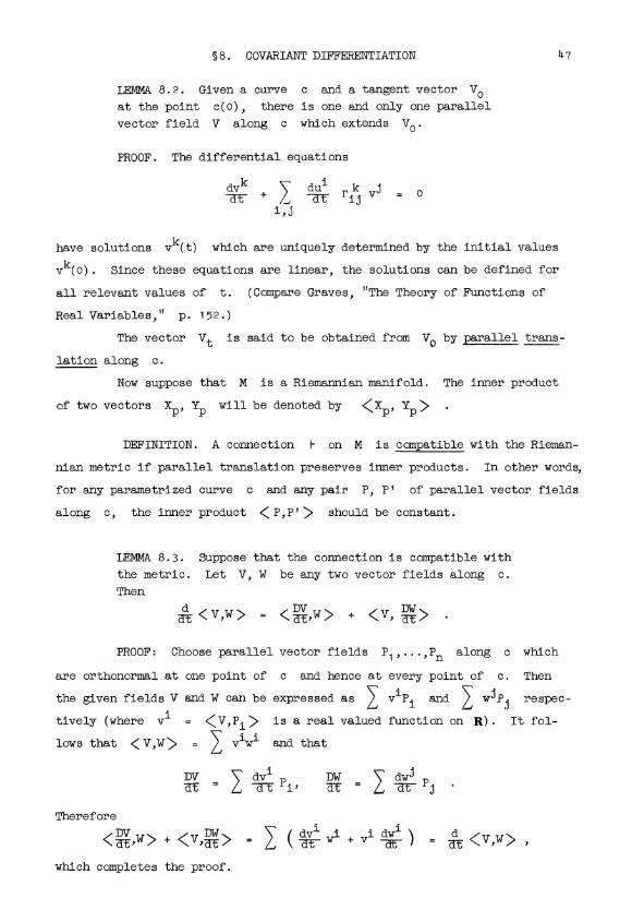
LEMMA 8.2. Given a curve c and a tangent vector V0
at the point c(o), there is one and only one parallel
vector field V along c which extends Vo.
PROOF. The differential equations
dvk+ du' r k vi = 0iji,j
47
have solutions vk(t) which are uniquely determined by the initial values
vk(o). Since these equations are linear, the solutions can be defined for
all relevant values of t. (Compare Graves, "The Theory of Functions of
Real Variables," p. 152.)
The vector Vt is said to be obtained from V0 by parallel trans-
lation along c.
Now suppose that M is a Riemannian manifold. The inner product
of two vectors Xp, Yp will be denoted by < Xp, Yp > .
DEFINITION. A connection F on M is compatible with the Rieman-
nian metric if parallel translation preserves inner products. In other words,
for any parametrized curve c and any pair P, P' of parallel vector fields
along c, the inner product < P,P' > should be constant.
LEMMA 8.3. Suppose that the connection is compatible with
the metric. Let V, W be any two vector fields along c.
Then
E < V,W > _ <Ur,W> + <V, UE> .
PROOF: Choose parallel vector fields P1,...,Pn along c which
are orthonormal at one point of c and hence at every point of c. Then
the given fields V and W can be expressed as I v1Pi and wiPj respec-
tively (where v1 = < V,Pi > is a real valued function on R). It fol-
lows that < V,W > _ >, v'w' and that
DV dv1 DW dwJPi, T£ _
P
Therefore< ,W> + <VrUT
_d i
wi + v1 d i \_dT ) =
d<V,W>
which completes the proof.
48 II. RIEMANNIAN GEOMETRY
COROLLARY 8.4. For any vector fields Y,Y' on M and anyvector XP e TMp:
Xp <Y,Y' > _ <Xp F Y,YY> + <Yp,Xp F Y' > .
PROOF. Choose a curve c whose velocity vector at t = 0 is Xp;
and apply 8.3.
DEFINITION 8.5. A connection F is called symmetric if it satis-
fies the identity*
(X F Y) - (Y F X) = [X,Y] .
(As usual, [X,Y] denotes the poison bracket [X,Y]f = X(Yf) - Y(Xf) of
two vector fields.) Applying this identity to the case X = ai, Y = aJ,
since [ai,ajl = 0 one obtains the relation
rij - rjk = o.
Conversely if ik = rji then using formula (6) it is not difficult to
verify that the connection F is symmetric throughout the coordinate neigh-
borhood.
LEMMA 8.6. (Fundamental lemma of Riemannian geometry.)
A Riemannian manifold possesses one and only one sym-
metric connection which is compatible with its metric.
(Compare Nomizu p. 76, Laugwitz p. 95.)
PROOF of uniqueness. Applying 8.4 to the vector fields ai,a3,ak,
and setting < aj,ak > = gjk one obtains the iaentity
ai gjk = < ai F apak > + < aj,ai F ak > .
Permuting i,j, and k this gives three linear equations relating the
*The following reformulation may (or may not) seem more intuitive. Define
The "covariant second derivative" of a real valued function f along two
vectors XpYp to be the expression
Xp(Yf) - (Xp F Y)f
where Y denotes any vector field extending Yp. It can be verified that
this expression does not depend on the choice of Y. (Compare the proof of
Lemma 9.1 below.) Then the connection is symmetric if this second deriva-
tive is symmetric as a function of Xp and Yp.
§8. COVARIANT DIFFERENTIATION 49
three quantities
< i F aj,akKaj k'ai>, and <ak F aj>
(There are only three such quantities since ai F 3j = aj F ai .) These
equations can be solved uniquely; yielding the first Christoffel identity
ai F aj,ak > = 2 (aigjk + ajgik - akgij) .
The left hand side of this identity is equal to rij gkk . Multiplying
P
by the inverse (g' ) of the matrix (gQk) this yields the second Christof-
fel identity
r j = 2 \ai gjk + aj gik - ak gij) gk¢
k
Thus the connection is uniquely determined by the metric.
Conversely, defining rl by this formula, one can verify that the
resulting connection is symmetric and compatible with the metric. This
completes the proof.
An alternative characterization of symmetry will be very useful
later. Consider a "parametrized surface" in M: that is a smooth function
s: R2 - M
By a vector field V along s is meant a function which assigns to each
(x,y) a R2 a tangent vector
V(x,Y) c TM5(x,Y)
As examples, the two standard vector fields
xand TV give rise to vec-
tor fields s, . and s* along s. These will be denoted briefly by-jV
Jx and y ; and called the "velocity vector fields" of s.
For any smooth vector field V along s the covariant derivatives
and are new vector fields, constructed as follows. For each fixedTy-
yo, restricting V to the curve
x s(x,Y0)
one obtains a vector field along this curve. Its covariant derivative with
respect to x is defined to be ()(xY) This defines along-DV'o
the entire parametrized surface s.
As examples, we can form the two covariant derivatives of the two

50 II. RIEMANNIAN GEOMETRY
vector fields as and as The derivatives D as and D as arecTx 3y Tx cTy cTy
simply the acceleration vectors of suitable coordinate curves. However,
the mixed derivatives and D cannot be described so simply.
LEMMA 8.7. If the connection is symmetric then D as=
D asax ay ay ax
PROOF. Express both sides in terms of a local coordinate system,
and compute.
§9. THE CURVATURE TENSOR 51
§9. The Curvature Tensor
The curvature tensor R of an affine connection F measures the
extent to which the second covariant derivative ai F () j F Z) is sym-
metric in i and j. Given vector fields X,Y,Z define a new vector field
R(X,Y)Z by the identity*
R(X,Y) Z = -X F (Y F Z) + Y F (X F Z) + [X,Y1 F Z
LEMMA 9.1. The value of R(X,Y)Z at a point p E M
depends only on the vectors Xp,Yp,Zp at this point
p and not on their values at nearby points. Further-
more the correspondence
Xp,Yp,Zp R(Xp,Yp)Zp
from TMp x TMp x TMp to TMp is tri-linear.
Briefly, this lemma can be expressed by saying that R is a "tensor."
PROOF: Clearly R(X,Y)Z is a tri-linear function of X,Y, and Z.
If X is replaced by a multiple fX then the three terms -X F (Y F Z),
Y F (X F Z), [X,Y] F Z are replaced respectively byi) - fX F (Y F Z) ,
ii) (Yf) (X F Z) + fY F (X F Z)
iii) - (Yf)(X F Z) + f[X,Y1 F Z
Adding these three terms one obtains the identity
R(fX,Y) Z = fR(X,Y) Z .
Corresponding identities for Y and Z are easily obtained by similar
computations.
Now suppose that X = xiai, Y = y'aj , and Z = zk)k.
Then
R(X,Y)Z = R(xiai,yjaj)(zk) k)
xiy izk R(ai)aj)ak
*Nomizu gives R the opposite sign. Our sign convention has the advan-
tage that (in the Riemannian case) the inner product < Ro hl)i)aj,ak
coincides with the classical symbol Rhijk
52 II. RIEMANNIAN GEOMETRY
Evaluating this expression at p one obtains the formula
(R(X,Y)Z)p = x1(p)yj(p)zk(p)(R(ai,aj)ak)p
which depends only on the values of the functions xi,yJ,zk at p, and
not on their values at nearby points. This completes the proof.
Now consider a parametrized surface
s: R2,MGiven any vector field V along s. one can apply the two covariant dif-
ferentiation operators -& and D to V. In general these operators will
not commute with each other.
LEMMA 9.2. cTy 3x V Tx rTy V - R( TX_,Ty) V
PROOF: Express both sides in terms of a local coordinate system,
and compute, making use of the identity
a1 F (ai F ak) - ai F (ai F ak) = R(ai,ai )ak .
[It is interesting to ask whether one can construct a vector field
P along s which is parallel, in the sense that
_ 5 _ X _
P = - P = 0,
and which has a given value P(0 0) at the origin. In general no such,
vector field exists. However, if the curvature tensor happens to be zero
then P can be constructed as follows. Let P(x,o) be a parallel vector
field along the x-axis, satisfying the given initial condition. For each
fixed x0 letP(xo,y)
be a parallel vector field along the curve
y - s(x0,y) ,
having the right value for y = 0. This defines P everywhere along s.
Clearly P is identically zero; and ZX P is zero along the x-axis.
Now the identity
D D D D ( as as3yTxP TxF = R \3x'T P = 0
P = 0. In other words, the vector field D P isimplies that y zx-parallel along the curves
y s(x0,y)
§9. THE CURVATURE TENSOR 53
Since (3Dx P)(x 0) = 0, this implies that -x P is identically zero;o
and completes the proof that P is parallel along s.]
Henceforth we will assume that M is a Riemannian manifold, pro-
vided with the unique symmetric connection which is compatible with its
metric. In conclusion we will prove that the tensor R satisfies four
symmetry relations.
LEMMA 9.3. The curvature tensor of a Riemannian manifold
satisfies:
(1) R(X,Y)Z + R(Y,X)Z = 0
(2) R(X,Y)Z + R(Y,Z)X + R(Z,X)Y = 0(3) <R(X,Y)Z,W> + <R(X,Y)W,Z> = 0(4) <R(X,Y)Z,W> _ <R(Z,W)X,Y>
PROOF: The skew-symmetry relation (1) follows immediately from the
definition of R.
Since all three terms of (2) are tensors, it is sufficient to
prove (2) when the bracket products [X,Y], [X,ZI and [Y,Z1 are all
zero. Under this hypothesis we must verify the identity
X F (Y F Z) + Y F (X F Z)
Y F (Z F X) + Z F (Y F X)
Z F (X FY) + X F (Z FY) = o .
But the symmetry of the connection implies that
Y FZ - Z FY = [Y,ZI = 0 .
Thus the upper left term cancels the lower right term. Similarly the re-
maining terms cancel in pairs. This proves (2).
To prove (3) we must show that the expression < R(X,Y)Z,W > is
skew-symmetric in Z and W. This is clearly equivalent to the assertion
that
<R(X,Y)Z,Z> = 0
for all X,Y,Z. Again we may assume that [X,YI = 0, so that
R(X,Y)Z,Z > is equal to
- X F (Y F Z) + Y F (X F Z),Z> .

54 II. RIEMANNIAN GEOMETRY
In other words we must prove that the expression
<Y F (X F Z),Z>
is symmetric in X and Y.
Since [X,Y] = 0 the expression YX < Z,Z > is symmetric in X
and Y. Since the connection is compatible with the metric, we have
X < Z,Z > = 2 <X F Z,Z >
hence
YX <Z,Z> = 2 <Y F(X F Z),Z> + 2 <X F Z,Y F Z>But the right hand term is clearly symmetric in X and Y. Therefore
Y F (X F Z),Z > is symmetric in X and Y; which proves property (3).
Property (4) may be proved from (1), (2), and (3) as follows.
<R(X,Y)Z,W>
<R (Z,W)X,Y>
Formula (2) asserts that the sum of the quantities at the vertices
of shaded triangle W is zero. Similarly (making use of (1) and (3)) the
sum of the vertices of each of the other shaded triangles is zero. Adding
these identities for the top two shaded triangles, and subtracting the
identities for the bottom ones, this means that twice the top vertex minus
twice the bottom vertex is zero. This proves (4), and completes the proof.
§10. GEODESICS AND COMPLETENESS 55
§10. Geodesics and Completeness
Let M be a connected Riemannian manifold.
DEFINITION. A parametrized path
y: I -+ M,
where I denotes any interval of real numbers, is called a geodesic if the
acceleration vector field UE is identically zero. Thus the velocityTdf
identity_d£ af, , = 2 < UE ,
dy0
shown that the length uuof the velocity vector isH _H
constant along y. Introducing the arc-length function
s(t) = \ DD IIdt + constant
This statement can be rephrased as follows: The parameter t along a
geodesic is a linear function of the arc-length. The parameter t is actu-
ally equal to the arc-length if and only if Idyll= 1.
In terms of a local coordinate system with coordinates u1,...,un
a curve t-+ y(t) e M determines n smooth functions u1(t),...,un(t).
The equation -aE UE for a geodesic then takes the form
d2uk + r k (u1 un) dul duJ- o
i,J=1
The existence of geodesics depends, therefore, on the solutions of a certain
system of second order differential equations.
More generally consider any system of equations of the form
-11 =dt2
Here u stands for (ul,...,un) and FI stands for an n-tuple of C°°
functions, all defined throughout some neighborhood U of a point
en(u1,v1) a R
56 II. RIEMANNIAN GEOMETRY
EXISTENCE AND UNIQUENESS THEOREM 10.1. There exists a
neighborhood W of the point (u1,-v1) and a number
e > o so that, for each (u0V0) E W the differen-
tial equation
dt2(u' at)
has a unique solution t -; u(t) which is defined for
Iti < e, and satisfies the initial conditionsy
u(0) u0, - (0) v0
Furthermore, the solution depends smoothly on the in-
itial conditions. In other words, the correspondence
(u0,v0,t) -' u(t)from W x (-e,e) to R n is a C°° function of all
2n+1 variables.
iPROOF: Introducing the new variables vi = 3T this system of n
second order equations becomes a system of 2n first order equations:
du= V
dv =(u,V)_df
The assertion then follows from Graves, "Theory of Functions of Real Vari-
ables," p. 166. (Compare our §2.4.)
Applying this theorem to the differential equation for geodesics,
one obtains the following.
LEMMA 10.2. For every point p0 on a Riemannian
manifold M there exists a neighborhood U of p0
and a number e > 0 so that: for each p c U and
each tangent vector v E TMp with length < e
there is a unique geodesic
7v: M
satisfying the conditions
dYv7 (o) = p, -- (0) = v
PROOF. If we were willing to replace the interval (-2,2) by an
arbitrarily small interval, then this statement would follow immediately
from 10.1. To be more precise; there exists a neighborhood U of p0 and
§10. GEODESICS AND COMPLETENESS 57
numbers E1,e2 > 0 so that: for each p E U and each v E TMp with
11vII < 51 there is a unique geodesic
yv: (-252,252) - M
satisfying the required initial conditions.
To obtain the sharper statement it is only necessary to observe that
the differential equation for geodesics has the following homogeneity pro-
perty. Let c be any constant. If the parametrized curve
t -F y(t)
is a geodesic, then the parametrized curve
t - y(ct)will also be a geodesic.
Now suppose that e is smaller than 5152. Then if ilvil < e and
Iti < 2 note that
IIv/5211 < 51 and le2tl <252 .
Hence we can define yv(t) to be yv/e2(e2t) . This proves 10.2.
This following notation will be convenient. Let V E TMq be a
tangent vector, and suppose that there exists a geodesic
y: [0,11 M
satisfying the conditions
y(o) = q, -(o) = v.
Then the point y(1) E M will be denoted by expq(v) and called the
exponential of the tangent vector v. The geodesic y can thus be des-
cribed by the formula
y(t) = expq(ty) .
The historical motivation for this terminology is the following. If M
is the group of all n x n unitary matrices then the tangent space TMI
at the identity can be identified with the space of n x n skew-Hermitian
matrices. The function
expl: TMI -. M
as defined above is then given by the exponential power series
expl(A) = I + A + 2 A2 +1
A3 + ...
58 II. RIEM&NNIAN GEOMETRY
Lemma 10.2 says that expq(v) is defined providing that IIvjj is small enough.
In general, expq(v) is not defined for large vectors v. However, if
defined at all, expq(v) is always uniquely defined.
DEFINITION. The manifold M is geodesically complete if expq(v)
is defined for all q E M and all vectors v E TMq. This is clearly equiva-
lent to the following requirement:
For every geodesic segment yo: [a,b] - M it should be possible
to extend 70 to an infinite geodesic
y : R - M .
We will return to a study of completeness after proving some local results.
Let TM be the tangent manifold of M, consisting of all pairs
(p,v) with p E M, v E TMp. We give TM the following COO structure:
if (u1,...,un) is a coordinate system in an open set U C M then every
tangent vector at q E U can be expressed uniquely as t1 a1 +...+ tnan,
where aiI
Then the functions uconstituteau q
a coordinate system on the open set TU C TM.
Lemma 10.2 says that for each p E M the map
(q,v) - expq(v)
is defined throughout a neighborhood V of the point (p,o) E TM. Further-
more this map is differentiable throughout V.
Now consider the smooth function F: V - M x M defined by
F(q,v) = (q, expq(v)). We claim that the Jacobian of F at the point
(p,o) is non-singular. In fact, denoting the induced coordinates on
U x U C M x M by u 2), we have
a aF(
au _ +u2
a aF* T =
au?
Thus the Jacobian matrix of F at (p,o) has the form ( o I 1 , and
hence is non-singular.
It follows from the implicit function theorem that F maps some
neighborhood V' of (p,o) E TM diffeomorphically onto some neighborhood
§10. GEODESICS AND COMPLETENESS 59
of (p,p) e M X M. We may assume that the first neighborhood v, consists
of all pairs (q,v) such that q belongs to a given neighborhood U' of
p and such that livII < s. Choose a smaller neighborhood W of p so that
F(V') D W x W. Then we have proven the following.
LEMMA 10.3. For each p e M there exists a neighborhood
W and a number e > 0 so that:
(1) Any two points of W are joined by a unique
geodesic in M of length < e.
(2) This geodesic depends smoothly upon the two
points. (I.e., if t -r exp q1(tv), 0 < t < 1, is the
geodesic joining q1 and q2, then the pair (q1,v) e
TM depends differentiably on (g1,g2).)
(3) For each q e W the map expq maps the open
e-ball in TMq diffeomorphically onto an open set
Uq) W.
REMARK. With more care it would be possible to choose W so that
the geodesic joining any two of its points lies completely within W. Com-
ptre J. H. C. Whitehead, Convex regions in the geometry of paths, Quarter-
ly Journal of Mathematics (Oxford) Vol. 3, (1932), pp. 33-42.
Now let us study the relationship between geodesics and arc-length.
THEOREM 10.4. Let W and e be as in Lemma 10.3. Let
y: [0,1]- Mbe the geodesic of length < e joining two points of W,
and letw: [0,1]- M
be any other piecewise smooth path joining the same two
points. Then,1 1
SlI IIdt< SII Udt
0 0
where equality can hold only if the point set w([o,1])
coincides with y([0,1]).
Thus y is the shortest path joining its end points.
The proof will be based on two lemmas. Let q = y(o) and let Uq
be as in 10.3.
6o II. RIEMANNIAN GEOMETRY
LEMMA 10.5. In Uq, the geodesics through q are
the orthogonal trajectories of hypersurfaces
expq(v) : v e TMq, IIvii = constant}
PROOF: Let t -+ v(t) denote any curve in TMq with 11v(t)II 1.
We must show that the corresponding curves
t -+ expq(rov(t) )
in Uq, where 0 < ro < e, are orthogonal to the radial geodesics
r -+ expq(rv(t0)) .
In terms of the parametrized surface f given by
f(r,t) = expq(rv(t)), 0 < r < e ,
we must prove that
<T,> =o-5 E
for all (r,t).
Now
a of of D of of of D ofFr Nr,a't> _ < cTr cTr'3f> + <Tr'Tr ; E> .
The first expression on the right is zero since the curves
r -+ f(r,t)are geodesics. The second expression is equal to
of D of > a of of = 0<i,-JE .> = 2 aEsince IIII = IIv(t) II = 1. Therefore the quantity <,> is indepen-CTF -H
dent of r. But for r = o we have
f(o,t) = expq(0) = q
hence M(0,t) = 0. Therefore < , > is identically zero, which com-Fr- 7Epletes the proof.
Now consider any piecewise smooth curve
CO: [a,bl -+ Uq - (q)Each point w(t) can be expressed uniquely in the form expq(r(t)v(t)) with
o < r(t) < e, and IIv(t) II = 1, v(t) e TMq.
LEMMA 10.6. The length IIdII dt is greater than ora
equal to Ir(b) - r(a)I, where equality holds only if the
function r(t) is monotone, and the function v(t) is constant.

§10. GEODESICS AND COMPLETENESS 61
Thus the shortest path joining two concentric spherical shells
around q is a radial geodesic.
Then
Since
PROOF: Let f(r,t) expq(rv(t)), so that m(t) = f(r(t),t)
dm afr,(t) +afCIE = cTr 3E
the two vectors on the right are mutually orthogonal, and since
1, this gives
II II2= Ir'(t)12 +
IIII2 > Ir'(t)12
where equality holds only if = 0; hence only if dv = 0. Thus
b b
S -Ildt > S Ir'(t) Idt > Ir(b) - r(a) Ia a
where equality holds only if r(t) is monotone and v(t) is constant.
This completes the proof.
The proof of Theorem 10.4 is now straightforward. Consider any
piecewise smooth path m from q to a point
q' = expq(rv) E Uq
where 0 < r < e, IvIi = 1. Then for any s > o the path m must con-
tain a segment joining the spherical shell of radius s to the spherical
shell of radius r, and lying between these two shells. The length of this
segment will be > r - s; hence letting s tend to 0 the length of m
will be > r. If m([0,1]) does not coincide with y([0,1)), then we
easily obtain a strict inequality. This completes the proof of 10.4.
An important consequence of Theorem 1o.4 is the following.
COROLLARY 10.7. Suppose that a path co: [o,A] - M, para-
metrized by arc-length, has length less than or equal to
the length of any other path from m(0) to m(A). Then m
is a geodesic.
PROOF: Consider any segment of co lying within an open set W, as
above, and having length < e. This segment must be a geodesic by Theorem
10.4. Hence the entire path m is a geodesic.
DEFINITION. A geodesic y: [a,b] -r M will be called minimal if
62 II. RIEMANNIAN GEOMETRY
its length is less than or equal to the length of any other piecewise smooth
path joining its endpoints.
Theorem 10.4 asserts that any sufficiently small segment of a
geodesic is minimal. On the other hand a long geodesic may not be minimal.
For example we will see shortly that a great circle arc on the unit sphere
is a geodesic. If such an arc has length greater than n, it is certainly
not minimal.
In general, minimal geodesics are not unique. For example two anti-
podal points on a unit sphere are joined by infinitely many minimal geodesics.
However, the following assertion is true.
Define the distance p(p,q) between two points p,q e M to be the
greatest lower bound for the arc-lengths of piecewise smooth paths joining
these points. This clearly makes M into a metric space. It follows
easily from 10.4 that this metric is compatible with the usual topology of M.
COROLLARY 10.8. Given a compact set K C M there exists
a number 6 > 0 so that any two points of K with dis-
tance less than s are joined by a unique geodesic of
length less than s. Furthermore this geodesic is minimal;
and depends differentiably on its endpoints.
PROOF. Cover K by open sets Wa, as in 10.3, and let s be
small enough so that any two points in K with distance less than s lie
in a common Wa. This completes the proof.
Recall that the manifold M is geodesically complete if every geo-
desic segment can be extended indifinitely.
THEOREM 10.9 (Hopf and Rinow*). If M is geodesically
complete, then any two points can be joined by a minimal
geodesic.
PROOF. Given p,q e M with distance r > 0, choose a neighborhood
Up as in Lemma 10.3. Let S C Up denote a spherical shell of radius s < a
Compare p. 341 of G. de Rham, Sur la r6ductibilite d'un espace de
Riemann, Commentarii Math. Helvetici, Vol. 26 (1952); as well as H. Hopf and
W. Rinow, Ueber den Begriff der-vollstandigen differentialgeometrischen Flache,
Commentarii,Vol. 3 (1931), pp. 209-225.
§10. GEODESICS AND COMPLETENESS 63
about p. Since S is compact, there exists a point
p0 = expp(sv) , 11V II = 1,
on S for which the distance to q is minimized. We will prove that
expp(rv) = q.
This implies that the geodesic segment t -+ y(t) = expp(tv), 0 < t < r,
is actually a minimal geodesic from p to q.
The proof will amount to showing that a point which moves along the
geodesic y must get closer and closer to q. In fact for each t e [s,r]
we will prove that
(it) p(y(t),q) = r-t .
This identity, for t = r, will complete the proof.
First we will show that the equality (18) is true. Since every
path from p to q must pass through S, we have
p(p,q) = Min (p(p,s) + p(s,q)) = s + p(po,q)se S
Therefore p(p0,q) = r - s. Since p0 = y(s), this proves (1s).
Let t0 e [6,r] denote the supremum of those numbers t for which
(it) is true. Then by continuity the equality (it ) is true also.0
If to < r we will obtain a contradiction. Let S' denote a small spheri-
cal shell of radius s' about the point y(to); and let pp e S' be a
point of S' with minimum distance from q. (Compare Diagram 10.) Then
p(Y(t0),q) = p(s,q)) = 6' + p(pp,q)
hence
(2) p(po,q) = (r - t0) - 6'
We claim that po is equal to y(to + s'). In fact the triangle
inequality states that
p(p,pp') > p(p,q) - p(pp,q) = to + s'
(making use of (2)). But a path of length precisely to + s' from p to
po is obtained by following y from p to y(to), and then following
a minimal geodesic from y(t0) to po. Since this broken geodesic has
minimal length, it follows from Corollary 10.7 that it is an (unbroken)

64 II. REIMANNIAN GEOMETRY
geodesic, and hence coincides with y.
Thus y(to + s') = pp. Now the equality (2) becomes
(1 to+s')0(y(to + ,'),q) = r - (to + s')
This contradicts the definition of t0; and completes the proof.
Diagram 10.
As a consequence one has the following.
COROLLARY 10.10. If M is geodesically complete then
every bounded subset of M has compact closure. Con-
sequently M is complete as a metric space (i.e., every
Cauchy sequence converges).
PROOF. If X C M has diameter d then for any p E X the map
expp: TMp -+ M maps the disk of radius d in TMp onto a compact subset
of M which (making use of Theorem 10.9) contains X. Hence the closure
of X is compact.
Conversely, if M is complete as a metric space, then it is not
difficult, using Lemma 10.3, to prove that M is geodesically complete.
For details the reader is referred to Hopf and Rinow. Henceforth we will
not distinguish between geodesic completeness and metric completeness, but
will refer simply to a complete Riemannian manifold.
§10. GEODESICS AND COMPLETENESS 65
FAMILIAR EXAMPLES OF GEODESICS. In Euclidean n-space, Rn, with
the usual coordinate system x1,...,xn and the usual Riemannian metric
dx®® dx1 +...+ dxn ® dxn we have ri = 0 and the equations for a geo-
desic y, given by t- (x1(t),...,xn(t) become
d2xi
dt '
whose solutions are the straight lines. This could also have been seen as
follows: it is easy to show that the formula for arc length
S ( \ 2dti=1
coincides with the usual definition of aru length as the least upper bound
of the lengths of inscribed polygons; from this definition it is clear that
straight lines have minimal length, and are therefore geodesics.
The geodesics on Sn are precisely the great circles, that is, the
intersections of Sn with the planes through the center of Sn.
PROOF. Reflection through a plane E2 is an isometry I: Sn -+ Sn
whose fixed point set is C = Sn n E2. Let x and y be two points of C
with a unique geodesic C' of minimal length between them. Then, since I
is an isometry, the curve I(C') is a geodesic of the same length as C'
between I(x) = x and I(y) = y. Therefore C' = I(C'). This implies that
C' C C.
Finally, since there is a great circle through any point of Sn in
any given direction, these are all the geodesics.
Antipodal points on the sphere have a continium of geodesics of
minimal length between them. All other pairs of points have a unique geo-
desic of minimal length between them, but an infinite family of non-minimal
geodesics, depending on how many times the geodesic goes around the sphere
and in which direction it starts.
By the same reasoning every meridian line on a surface of revolution
is a geodesic.
The geodesics on a right circular cylinder Z are the generating
lines, the circles cut by planes perpendicular to the generating lines, and
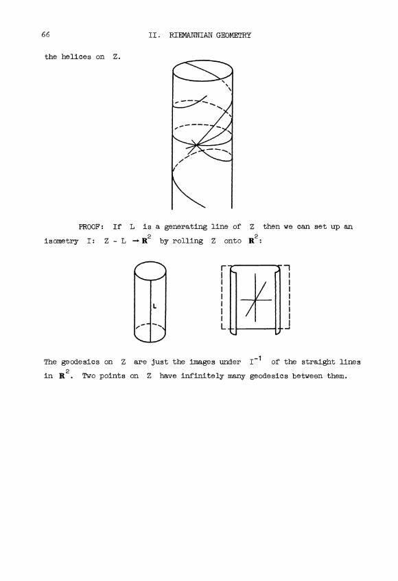
66 II. RIEMANNIAN GEOMETRY
the helices on Z.
PROOF: If L is a generating line of Z then we can set up an
isometry I: Z - L - R2 by rolling Z onto R2:
a 1
The geodesics on Z are just the images under I-1 of the straight lines
in R. Two points on Z have infinitely many geodesics between them.2

PART III
THE CALCULUS OF VARIATIONS APPLIED TO GEODESICS
§11. The Path Space of a Smooth Manifold.
Let M be a smooth manifold and let p and q be two (not neces-
sarily distinct) points of M. By a piecewise smooth path from p to q
will be meant a map w: [0,1] - M such that
1) there exists a subdivision 0 = to < t1 < ... < tk = 1 of
[0,1] so that each wl[ti_1,ti] is differentiable of class C
2) w(o) = p and w(1) = q.
The set of all piecewise smooth paths from p to q in M will be denoted
by 0(M;p,q), or briefly by 0(M) or 11.
Later (in §16) 0 will be given the structure of a topological
space, but for the moment this will not be necessary. We will think of a
as being something like an "infinite dimensional manifold." To start the
analogy we make the following definition.
By the tangent space of a at a path w will be meant the vector
space consisting of all piecewise smooth vector fields W along w for
which W(0) = 0 and W(1) = 0. The notation TOW will be used for this
vector space.
If F is a real valued function on 0 it is natural to ask what
F*: TQw - TRF(w) ,
the induced map on the tangent space, should mean. When F is a function
which is smooth in the usual sense, on a smooth manifold M, we can define
F*: TMp - T RKp) as follows. Given X E TMp choose a smooth path
u - a(u) in M, which is defined for -e < u < e , so that
a(0) = p, moo) = X
68 III. CALCULUS OF VARIATIONS
Then F*(X) is equal tod(F(a(u))I multiplied by the basis vectorTu u=o'
dUf )F (P) E TRF(p)
In order to carry out an analogqus construction for F: a - R,
the following concept is needed.
DEFINITION. A variation of m (keeping endpoints fixed) is a
function
a: (-e,e) -. 0,
for some e > o, such that
1) &(o) = m
2) there is a subdivision 0 = to < t1 < ... < tk = 1
of [0,11 so that the map
a: (-e,e) x [0,11 -+ M
defined by a(u,t) = &(u)(t) is C°° on each strip (-e,e) x [ti-1,ti
i = 1,...,k.
Since each &(u) belongs to Q = 0(M;p,q), note that:
3) a(u,o) = p, a(u,1) = q for all u e (-e,e) .
We will use either a or a to refer to the variation. More
generally if, in the above definition, (-e,e) is replaced by a neighbor-
hood U of 0 in Rn, then a (or a) is called an n-parameter varia-
tion of m.
Now a may be considered as a "smooth path" in 11. Its "velocity
vector" d. (o) e Tom is defined to be the vector field W along m givencTu
by
Wt = m(o)t =(o,t)Clearly W E T11m. This vector field W is also called the variation vec-
tor field associated with the variation a.
Given any W E Tom note that there exists a variation
(-e,e) - 11 which satisfies the conditions a(o) = to, mo(o) = W.
In fact one can set
&(u) (t) = expm(t)(u Wt) .
By analogy with the definition given above, if F is a real valued
§11. THE PATH SPACE
function on a, we attempt to define
F* : TO -+ TRF(m)
as follows. Given W e Tow choose a variation a: (-E,e) - 0 with
69
a(o) = w, mo(o) = W
and set F*(W) equal to d(F())lu=o multiplied by the tangent vectorCLU
d Of course without hypothesis on F there is no guarantee thatF(n)'
this derivative will exist, or will be independent of the choice of a.
We will not investigate what conditions F must satisfy in order for F*
to have these properties. We have indicated how F* might be defined only
to motivate the following.
DEFINITION. A path w is a critical path for a function
F: 0 -+ R if and only if dF( u I is zero for every variation a ofu=o
w.
EXAMPLE. If F takes on its minimum at a path mo, and if the
derivatives are all defined, then clearly mo is a critical path.(

70 III. CALCULUS OF VARIATIONS
§12. The Energy of a Path.
Suppose now that M is a Riemannian manifold. The length of a vec-i
for v E TMp will be denoted by IlvOO _ < v,v >2. For a e a define the
energy of co from a to b (where o < a < b < 1) as
Ea(m) =SI1-dfa
We will write E for E.
This can be compared with the arc-length from a to b given by
b
Lab ces) = S II IIdta
as follows. Applying Schwarz's inequality
with f(t) =
bl2
b blS fgdt) < \ S f 2dt') ( .S g2dt)
a a a
1 and g(t) = IIdo)
II
we see that
(Lb < (b - a)Ea ,
where equality holds if and only if g is constant; that is if and only if
the parameter t is proportional to arc-length.
Now suppose that there exists a minimal geodesic y from p = m(o)
to q = m(1). Then
E(y) = L ( - / ) L ( w ) .
Here the equality L(y)2 = L(m)2 can hold only if m is also a minimal
geodesic, possibly reparametrized. (Compare §10.7.) On the other hand
the equality L(w)2 = E(m) can hold only if the parameter is proportional
to arc-length along w. This proves that E(y) < E(m) unless a is also
a minimal geodesic. In other words:
LEMMA. 12.1. Let M be a complete Riemannian manifold
and let p,q e M have distance d. Then the energy
function
E: a(M;p,q) - R

§12. TEE ENERGY OF A PATH 71
takes on its minimum d2 precisely on the set of minimal
geodesics from p to q.
We will now see which paths m e 9 are critical paths for the
energy function E.
(o,t)Let a: (-e,e) - 2 be a variation of m, and let Wt =Tu-
be the associated variation vector field. Furthermore, let:
Vt =
UE= velocity vector of m
At DcT - = acceleration vector of m
otv = Vt. - Vt_ = discontinuity in the velocity vector at t,
where 0 < t < 1 .
Of course otV = 0 for all but a finite number of values of t.
THEOREM 12.2 (First variation formula). The derivative
1 dE(a(u))is equal to2 - u=o 1
- <Wt,AtV> - S <Wt,At> dtt 0
PROOF: According to Lemma 8.3, we have
as as D as asTu <-cf,ZT > = 2 < Tu Z'
Therefore
dE(a(u)) d ( 2 as, asTU- < as, as dt < D_ J > ) -3 -Z > dt
0 0
By Lemma 8.7 we can substitute D asfor
D as in this last formula.3ETu 3u 3TChoose 0 = t0 < t1 <...< tk = 1 so that a is differentiable on
each strip (-e,e) x [ti_1,ti1. Then we can "integrate by parts" on
[ti_1,til, as follows. The identity
as as D as as as D as-ate <uT
,> +
<au,
-3y >
implies that
ti
S 3E 3u ,3T > dt = < aa, aaTu3t>ti-1
(ti,1 <Tu, D )a
, 2T) 3E>dtti-1
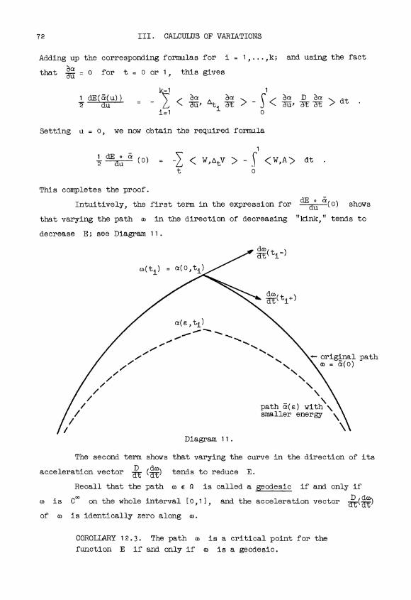
72 III. CALCULUS OF VARIATIONS
Adding up the corresponding formulas for i = 1,...,k; and using the fact
that u = o for t = 0 or 1, this gives
k-1 1
1 dE(a(u)) as as as D as2 u L < U, pti ] - < y.-, ZE ZE > dt
i=1 0
Setting u = 0, we now obtain the required formula
2 dE a (o) < W,AtV > - S < W,A > dtt 0
This completes the proof.
Intuitively, the first term in the expression for da(0) shows
that varying the path w in the direction of decreasing "kink," tends to
decrease E; see Diagram 11.
The second term shows that varying the curve in the direction of its
acceleration vector () tends to reduce E.
Recall that the path w e 0 is called a geodesic if and only if
w is C`° on the whole interval [0,11, and the acceleration vector -(
of w is identically zero along w.
COROLLARY 12.3. The path w is a critical point for the
function E if and only if co is a geodesic.
§12. THE ENERGY OF A PATH 73
PROOF: Clearly a geodesic is a critical point. Let m be a
critical point. There is a variation of m with W(t) = f(t)A(t) where
f(t) is positive except that it vanishes at the ti. Then
2 mo(o) _ - f(t) < A(t),A(t) > dt.0
This is zero if and only if A(t) = 0 for all t. Hence each nI[ti,ti+1]
is a geodesic.
Now pick a variation such that W(ti) = Ati V. Then
2 (0) _ - < AtiV,AtiV > . If this is zero then all AtV are 0, and
m is differentiable of class C1, even at the points ti. Now it follows
from the uniqueness theorem for differential equations that m is C°°
everywhere: thus co is an unbroken geodesic.
74 III. CALCULUS OF VARIATIONS
§13. The Hessian of the Energy Function at a Critical Path.
Continuing with the analogy developed in the preceding section, we
now wish to define a bilinear functional
E**: TOY x TOy - R
when y is a critical point of the function E, i.e., a geodesic. This
bilinear functional will be called the Hessian of E at y.
If f is a real valued function on a manifold M with critical
point p, then the Hessian
f**: TM p x TMp -+ R
can be defined as follows. Given X1,X2 E TMp choose a smooth map
(u1,u2) a(u1,u2) defined on a neighborhood of (0,0) in R2, with
values in M, so that
a(o,o) = p, X1(0,0) = x1 X2(0,0) = x2
Then
f**(X1,X2) =2f(a(u1,u2))
au1 au2(0,0)
This suggests defining E** as follows. Given vector fields W1,W2 e Tsar
choose a 2-parameter variation
a: U x [ 0 , 1 1 - M
where U is a neighborhood of (0,0) in R2, so that
a(o,o,t) = y(t), (o,o,t) = W1(t), au (0,0,t) = W2(t)1 2
(Compare §11.) Then the Hessian E**(W1,W2) will be defined to be the
second partial derivative
2E(a(ut,u2))I
auI au2(0 0),
where a(u1,u2) e 0 denotes the path a(u1,u2)(t) = a(u1,u2,t) . This
second derivative will be written briefly as o u2(0,0)1 2
The following theorem is needed to prove that E** is well defined.

§13. THE HESSIAN OF E
THEOREM 13.1 (Second variation formula). Let &: U -+sa
be a 2-parameter variation of the geodesic y with
variation vector fields
Wi = x,(0,0) e Tay, i = 1,2
Then the second derivative
function is equal to
1 a"E(0,0)2 u3 you
< W21
Therefore
0
CD as D as > dt< cTu1 Tu2 ) 3T 'R
0
Let us evaluate this expression for (u1,u2) = (0,0).
an unbroken geodesic, we have
asAt 3T =
0,D as
WE ZT
so that the first and third terms are zero.
(13.2)
where V = d denotes the velocity vector field and where
DW
- <W2(t),AtUU1> -St 0
ofd _(t+) -(t )DW
denotes the jump in at one of its finitely many-dy
points of discontinuity in the open unit interval.
PROOF: According to 12.2 we have1
1 aE<
as as as D as At2 3u2 = - cTu2,t > - S <Tu2, WE 3T >t 0
1 a2E D as acf u1 u2 = - < cTu1 3T > -t t
Rearranging the second term, we obtain
1 6 E 0 0)2 W2 At aE W1
In order to interchange the two operators D1
bring in the curvature formula,
D 2WI + R(V,W1)V > dt
of the energy
75
as D as >2 P 1 At 'R
as D D as37
0
Since y = &(0,0) is
e
-)
< W2, 1 -RV > dt0
and 3 , we need to
dt.
1)V = R(V,W1)V1 D V - A 1V = R( 4,Tu-
76 III. CALCULUS OF VARIATIONS
Together with the identity V = 3U T_ =_CTU
W1 this yields1 1
DST(13.3) 1 D V =
d+ R(V,W1)V
_3Tff
Substituting this expression into (13.2) this completes the proof of 13.1.2
COROLLARY 13.1+. The expression E**(W1,W2) = )E-2(0,0)
is a well defined symmetric and bilinear function of W
and W2.
PROOF: The second variation formula shows that ua u 7-0, 0)1 2
depends only on the variation vector fields W1 and W2, so that
E**(W1,W2) is well defined. This formula also shows that E** is bilinear.
The symmetry property
E**(W1,W2) = E**(W2, W1)
is not at all obvious from the second variation formula; but does follow
immediately from the symmetry property aE =6 E
u1 u2 uc 7 1
REMARK 13.5. The diagonal terms E**(W,W) of the bilinear pairing
E** can be described in terms of a 1-parameter variation of y. In fact
E**(W,W) = d E a(o)
where a: (-e,e) -+s1 denotes any variation of y with variation vector
field T- (o) equal to W. To prove this identity it is only necessary to
introduce the two parameter variation
(u1,u2) = a(u1 + u2)
and to note that
a9 da a2E ° d2E ° au=ci' ut = d2As an application of this remark, we have the following.
LEMMA 13.6. If y is a minimal geodesic from p to q
then the bilinear pairing E** is positive semi-definite.
Hence the index X of E** is zero.
PROOF: The inequality E(a(u)) > E(y) = E(a(o)) implies that
d2E(a( , evaluated at u = 0, is > 0. Hence E**(W,W) > 0 for all W.

§14. JACOBI FIELDS
§14. Jacobi Fields: The Null Space of E**
A vector field J along a geodesic y is called a Jacobi field
if it satisfies the Jacobi differential equation
2
D + R(V,J)V = odt
77
where V = Ur . This is a linear, second order differential equation.
[It can be put in a more familiar form by choosing orthonormal parallel vec-
tor fields P1,...,Pn along y. Then setting J(t) = E fi(t)Pi(t), the
equation becomes
2 ida+ L a'(t)fj(t) = o, i = 1,..., n;
j=1
where a3 = < R(V,Pj)V,Pi > .] Thus the Jacobi equation has 2n linearly
independent solutions, each of which can be defined throughout y. The
solutions are all C°°-differentiable. A given Jacobi field J is com-
pletely determined by its initial conditions:
J(o), uE(o) e TM'Y(0)
Let p = y(a) and q = y(b) be two points on the geodesic y,
with a b.
DEFINITION. p and q are conjugate* along y if there exists a
non-zero Jacobi field J along y which vanishes for t = a and t = b.
The multiplicity of p and q as conjugate points is equal to the dimen-
sion of the vector space consisting of all such Jacobi fields.
Now let y be a geodesic in S2 = S0(M;p,q). Recall that the null-
space of the Hessian
E**: TOY x TOy--. R
is the vector space consisting of those W1 e TOy such that E**(W1,W2) = 0
*If y has self-intersections then this definition becomes ambiguous.
One should rather say that the parameter values a and b are conjugate
with respect to y.
78 III. CALCULUS OF VARIATIONS
for all W2. The nullity v of E** is equal to the dimension of this
null space. E** is degenerate if v > 0.
THEOREM 14.1. A vector field W1 e TOy belongs to the
null space of E** if and only if W1 is a Jacobi field.
Hence E** is degenerate if and only if the end points
p and q are conjugate along y. The nullity of E** is
equal to the multiplicity of p and q as conjugate points.
PROOF: (Compare the proof of 12.3.) If J. is a Jacobi field which
vanishes at p and q, then J certainly belongs to TOO. The second
variation formula (§13.1) states that
Cl
t 0
Hence J belongs to the null space.
Conversely, suppose that W1 belongs to the null space of E**.
Choose a subdivision o = t0 < t1 <...< tk = 1 of [0,11 so that
W1l[ti_1,ti1 is smooth for each i. Let f: [0,11 -+ [0,11 be a smooth
function which vanishes for the parameter values t0,t1,...,tk and is
positive otherwise; and let
D2W
W2(t) = f(t)( 2 + R(VW1)V)tdt
Then
2W 21
E + R(V,W1)VII dt- 2E**(W1,W2)=
0 + f(t)t1o
Since this is zero, it follows that W1j[ti-1,ti1 is a Jacobi field for
each i.
I
Now let W2 e TOOy be a field such that W2(ti)DW1
= At -- fori
i = 1,2,...,k-1. Then
- 2E**(W1,WI)
k-1
i=1
DW1Ati .-
2 1
+ 0 dt = 00
DW1Hence -cTE has no jumps. But a solution W1 of the Jacobi equation is
completely determined b the vectors W andDW1
by 1(ti) Ur-(ti). Thus it fol-
lows that the k Jacobi fields W11[ti_1,ti1, i = 1,...,k, fit together
to give a Jacobi field W1 which is C`°-differentiable throughout the

§14. JACOBI FIELDS 79
entire unit interval. This completes the proof of 14.1.
It follows that the nullity v of E** is always finite. For
there are only finitely many linearly independent Jacobi fields along y.
REMARK 14.2. Actually the nullity v satisfies 0 < v < n. Since
the space of Jacobi fields which vanish for t = 0 has dimension
precisely n, it is clear that v < n. We will construct one
example of a Jacobi field which vanishes for t = 0, but not for
t = 1. This will imply that v < n. In fact let Jt = tVt where
V = 7 denotes the velocity vector field. Then
DJ(IT
1 V+ t DV = V
2
(Since
Uy= o), hence = 0. Furthermore R(V,J)V = tR(V,V)V
dt7= 0 since R is skew symmetric in the first two variables. Thus
J satisfies the Jacobi equation. Since J0 = 0, J1 # 0, this
completes the proof.
EXAMPLE 1. Suppose that M is "flat" in the sense that the curva-
ture tensor is identically zero. Then the Jacobi equation becomes
dt2 = 0. Setting J(t) =) fi(t)Pi(t) where Pi are parallel,
2 ithis becomes ddf7 = 0. Evidently a Jacobi field along y can have
at most one zero. Thus there are no conjugate points, and E** is
non-degenerate.
EXAMPLE 2. Suppose that p and q are antipodal points on the
unit sphere Sn, and let y be a great circle arc from p to q.
Then we will see that p and q are conjugate with multiplicity
n-1. Thus in this example the nullity v of E** takes its
largest possible value. The proof will depend on the following
discussion.
Let a be a 1-parameter variation of y, not necessarily keeping
the endpoints fixed, such that each &(u) is a geodesic. That is, let
a: x [0,11 -+ M
be a COO map such that a(o,t) = y(t), and such that each a(u) [given
by &(u)(t) = a(u,t)] is a geodesic.

80 III. CALCULUS OF VARIATIONS
LEMMA 14.3. If a is such a variation of y through
geodesics, then the variation vector field W(t) _(O,t)
is a Jacobi field along Y.
PROOF: If a is a variation of y through geodesics, thenD asdT3£
is identically zero. Hence
D D as D D as R( as as \ as0 ° Tu3-E3y - 3TTu 3T + CTU ZE
D2 as as a(X ) as
+ R\.t'Tu at
(Compare §13.3.) Therefore the variation vector field Y is a Jacobi
field.
Thus one way of obtaining Jacobi fields is to move geodesics around.
Now let us return to the example of two antipodal points on a unit
n-sphere. Rotating the sphere, keeping p and q fixed, the variation
vector field along the geodesic y will be a Jacobi field vanishing at p
and q. Rotating in n-1 different directions one obtains n-1 linearly
independent Jacobi fields. Thus p and q are conjugate along y with
multiplicity n-1.

§14. JACOBI FIELDS 81
LEMMA 14.4. Every Jacobi field along a geodesic y: [0,11-+ M
may be obtained by a variation of y through geodesics.
PROOF: Choose a neighborhood U of y(o) so that any two points
of U are joined by a unique minimal geodesic which depends differentiably
on the endpoints. Suppose that y(t) e U for 0 < t < s. We will first
construct a Jacobi field W along yl[o,s] with arbitrarily prescribed
values at t = 0 and t = s. Choose a curve a: (-e,E) -+ U so that
a(o) = y(o) and so that mo(o) is any prescribed vector in TM y(0).
Similarly choose b: (-E,E) -+ U with b(0) y(s) and T(o) arbitrary.
Now define the variation
a: (-E,E) x [o,s] -+ M
by letting a(u): M be the unique minimal geodesic from a(u)
to b(u). Then the formula t -+(o,t) defines a Jacobi field with the(TU
given end conditions.
Any Jacobi field along yl[o,s] can be obtained in this way: If
7(y) denotes the vector space of all Jacobi fields W along y, then the
formula W (W(0), W(s)) defines a linear map
f: 7(y) -+ TMY(0) X TM7(s)We have just shown that f is onto. Since both vector spaces have the same
dimension 2n it follows that f is an isomorphism. I.e., a Jacobi field
is determined by its values at y(o) and y(s). (More generally a Jacobi
field is determined by its values at any two non-conjugate points.) There-
fore the above construction yields all possible Jacobi fields along
yl[o,s1.
The restriction of a(u) to the interval 10,81 is not essential.
If u is sufficiently small then, using the compactness of [0,11, a(u)
can be extended to a geodesic defined over the entire unit interval [0,11.
This yields a variation through geodesics:
a&: (-E',E') X [0,11 -+ M
with any given Jacobi field as variation vector.
REMARK 14.5. This argument shows that in any such neighborhood U
the Jacobi fields along a geodesic segment in U are uniquely determined
82 III. CALCULUS OF VARIATIONS
by their values at the endpoints of the geodesic.
REMARK 14.6. The proof shows also, that there is a neighborhood
(-S,s) of 0 so that if t e (-s,s) then y(t) is not conjugate to
y(o) along y. We will see in §15.2 that the set of conjugate points to
y(o) along the entire geodesic y has no cluster points.

§15. THE INDEX THEOREM 83
§15. The Index Theorem.
The index % of the Hessian
E**: TOy x TOy-+ R
is defined to be the maximum dimension of a subspace of Tay on which E**
is negative definite. We will prove the following.
THEOREM 15.1 (Morse). The index X of E** is equal
to the number of points y(t), with 0 < t < 1, such
that y(t) is conjugate to y(o) along y; each such
conjugate point being counted with its multiplicity.
This index . is always finite*.
As an immediate consequence one has:
COROLLARY 15.2. A geodesic segment y: [0,11 - M can
contain only finitely many points which are conjugate
to y(o) along y.
In order to prove 15.1 we will first make an estimate for ) by
splitting the vector space Tay into two mutually orthogonal subspaces, on
one of which E** is positive definite.
Each point y(t) is contained in an open set U such that any two
points of U are joined by a unique minimal geodesic which depends differ-
entiably on the endpoints. (See §10.) Choose a subdivision
o = to < t1 ..< tk = 1 of the unit interval which is sufficiently fine
so that each segment y[ti_i,til lies within such an open set U; and so
that each yl[ti_1,tiI is minimal.
Let TOy(to,tl,t2,...,tk) C TOy be the vector space consisting of
all vector fields W along y such that
1) WI[ti_i,til is a Jacobi field along yl[ti_1,tiI for each i;
2) W vanishes at the endpoints t = 0, t = 1.
Thus T11y(t0,tl,...,tk) is a finite dimensional vector space consisting of
broken Jacobi fields along y.
*For generalization of this result see: W. Ambrose, The index theorem in
Riemannian geometry, Annals of Mathematics, Vol. 73 (1961), pp. 49-86.
84 III. CALCULUS OF VARIATIONS
Let T' C Tsar be the vector space consisting of all vector fields
W E TOY for which W(t0) = 0, W(t1) = 0, W(t2) = 0,..., W(tk) = o.
LEMMA 15.3. The vector space Tsar splits as the direct
sum TOy(to,t,,...,tk) ® T'. These two subspaces are
mutually perpendicular with respect to the inner product
E**. Furthermore, E** restricted to T' is positive
definite.
PROOF: Given any vector field W E TOY let W1 denote the unique
"broken Jacobi field" in TOy(t0,t1,...,tk) such that W1(ti) = W(ti) for
i = 0,1,...,k. It follows from §14.5 that W1 exists and is unique.
Clearly W - W1 belongs to T'. Thus the two subspaces, Tsay(to,t1,...,tk)
and T' generate Tsar, and have only the zero vector field in common.
If W1 belongs to Tsay(to)tl,...,tk) and W2 belongs to T',
then the second variation formula (13.1) takes the form
1
LW
-liE**(Wj<W2(t),pt -1 > - <W2,o > dt = 0
t 0
Thus the two subspaces are mutually perpendicular with respect to E**
For any W E TO the Hessian E**(W,W) can be interpreted as the2
second derivative d E
y
2 a (0); where &: (-s,e) is any variation of7,
y with variation vector field mo(o) equal to W. (Compare 13.5.) If
W belongs to T' then we may assume that & is chosen so as to leave the
points y(to),y(t1),...,y(tk) fixed. In other words we may assume that
a(u)(ti) = y(ti) for i = 0,1,...,k.
Proof that E**(W,W) > 0 for W e T'. Each a(u) e 0 is a piece-
wise smooth path from y(o) to y(t1) to y(t2) to ... to y(1). But
each yl[ti_1,ti] is a minimal geodesic, and therefore has smaller energy
than any other path between its endpoints. This proves that
E(a(u)) > E(y) = E(a(o)) .
Therefore the second derivative, evaluated at u = 0, must be > 0.
Proof that E**(W,W) > 0 for W E T', W 0. Suppose that
E**(W,W) were equal to 0. Then W would lie in the null space of E**.
In fact for any W1 e T0y(t0,t1,...,tk) we have already seen that
E**(W1,W) = 0. For any W2 e T' the inequality
§15. THE INDEX THEOREM 85
0 < E**(W + c W2, W + c W2) = 2c E**(W2,W) + C2E**(W2,W2)
for all values of c implies that E**(W2,W) = 0. Thus W lies in the
null space. But the null space of E** consists of Jacobi fields. Since
T' contains no Jacobi fields other than zero, this implies that W = 0.
Thus the quadratic form E** is positive definite on T'. This
completes the proof of 15.3.
An immediate consequence is the following:
LEMMA 15.4. The index (or the nullity) of E** is equal
to the index (or nullity) of E** restricted to the space
TOy(t0,t1,...,tk) of broken Jacobi fields. In particular
(since To7(t0,tl,...,tk) is a finite dimensional vector
space) the index X is always finite.
The proof is straightforward.
Let yT denote the restriction of y to the interval [O,T].
Thus yT: [O,T] -+ M is a geodesic from y(o) to y(T). Let ?(T) denote
the index of the Hessian ( Eo )** which is associated with this geodesic.
Thus X(1) is the index which we are actually trying to compute. First
note that:
ASSERTION (1). X(T) is a monotone function of T.
For if T < T' then there exists a X(T) dimensional space P of
vector fields along yT which vanish at y(o) and y(T) such that the
Hessian ( Eo )** is negative definite on this vector space. Each vector
field in '' extends to a vector field along yT' which vanishes identically
between y(T) and y(T'). Thus we obtain a X(T) dimensional vector space
of fields along yT,
%(T) <
on whichEoi
)** is negative definite. Hence
ASSERTION (2). T.(-T) = 0 for small values of T.
For if T is sufficiently small then yT is a minimal geodesic,
hence X(T) = 0 by Lemma 13.6.
Now let us examine the discontinuities of the function X(T). First
note that X(T) is continuous from the left:
ASSERTION (3). For all sufficiently small e > 0 we have
A.(T-E) = X(T).
86 III. CALCULUS OF VARIATIONS
PROOF. According to 15.3 the number x(1) can be interpreted as
the index of a quadratic form on a finite dimensional vector space
T0y(to,t1,...,tk). We may assume that the subdivision is. chosen so that
say ti < T < ti+1. Then the index X(T) can be interpreted as the index
of a corresponding quadratic form HT on a corresponding vector space of
broken Jacobi fields along yT. This vector space is to be constructed
using the subdivision 0 < t1 < t2 <... < ti < T of [0,T1. Since a
broken Jacobi field is uniquely determined by its values at the break points
y(ti), this vector space is isomorphic to the direct sum
E = TMy(t1) ® TMy(t2) ® ... ® TMy(ti) .
Note that this vector space E is independent of T. Evidently the quad-
ratic form H. on E varies continuously with T.
Now HT is negative definite on a subspace V C E of dimension
X(T). For all r' sufficiently close to T it follows that HT, is
negative definite on V. Therefore X(T') > But if T' = T - e < T
then we also have ?V(T-e) < >,(T) by Assertion 1. Hence 'X(T-e) _ X(T).
ASSERTION (4). Let v be the nullity of the Hessian ( Eo ).
Then for all sufficiently small e > 0 we have
.l.(T+e) = x(T) + V
Thus the function x(t) jumps by v when the variable t passes
a conjugate point of multiplicity v; and is continuous otherwise. Clearly
this assertion will complete the proof of the index theorem.
PROOF that a(T+e) < X(T) + v . Let HT and E be as in the proof
of Assertion 3. Since dim E = ni we see that H. is positive definite on
some subspace )' C Z of dimension ni - X(T) - v. For all T' sufficient-
ly close to T, it follows that HT, is positive definite on n". Hence
X(T') < dim E - dime" l.(T) + v
PROOF that X(T+e) > X(T) + v. Let W1,-..,wx(T) be X(T) vector
fields along yT, vanishing at the endpoints, such that the matrix
( Ep )+ (Wi,Wj) 1
§15. THE INDEX THEOREM 87
is negative definite. Let J1,...,J, be v linearly independent Jacobi
fields along yT, also vanishing at the endpoints. Note that the v
vectorsDJh-HE('r) E TMY(T)
are linearly independent. Hence it is possible to choose v vector fields
X1, ... ,X, along YT+E' vanishing at the endpoints of rT + E, so that
(DJh \\
dt
is equal to the v x v identity matrix. Extend the vector fields Wi and
Jh over yT+E by setting these fields equal to 0 for T < t < T + E.
Using the second variation formula we see easily that
ToeEo )**
Jh' WO = o
Eo+EI**( Jh' Xk) = 2shk (Kronecker delta).
Now let c be a small number, and consider the X(T) + v vector fields
W1,...,Wx(T),c_1
J1 - c X1,..., c_1Jv - c Xv
along YT+E' We claim that these vector fields span a vector space of
dimension )(T) + v on which the quadratic form ( E"'),, is negative
definite. In fact the matrix of (Eo+E)** with respect to this basis is
ET )**( WI,W c A
c At -4I+ c 2B /
where A and B are fixed matrices. If c is sufficiently small, this
compound matrix is certainly negative definite. This proves Assertion (4).
The index theorem 15.1 clearly follows from the Assertions (2),(3),
and (4) .
88 III. CALCULUS OF VARIATIONS
§16. A Finite Dimensional Approximation to 0c
Let M be a connected Riemannian manifold and let p and q be
two (not necessarily distinct) points of M. The set a = 0(M;p,q) of
piecewise C°° paths from p to q can be topologized as follows. Let p
denote the topological metric on M coming from its Riemann metric. Given
w, W' e n with arc-lengths s(t), s'(t) respectively,define the distance
d(W,W') to be1 i2
Max p(a(t), W'(t)) +L
C r .ds'\ dt]z
0< t< 1 \ / L J0 \ 1
(The last term is added on so that the energy function
2
Eb(W) = ( ddt
a
will be a continuous function from a to the real numbers.) This metric
induces the required topology on D.
Given c > 0 let 0c denote the closed subset E-1([O,cl) C n
and let Int Sac denote the open subset E-1([o,c)) (where E = E1: n - R
is the energy function). We will study the topology of nc by construct-
ing a finite dimensional approximation to it.
Choose some subdivision 0 = to< t1 <...< tk = I of the unit inter-
val. Let Sa(to,t1,...,tk) be the subspace of a consisting of paths
W: (0,11 - M such that1) a(o) = p and a)(1) =q2) ml[ti-1,ti) is a geodesic for each i = 1,...,k.
Finally we define the subspaces
n(to,t1,...,tk)c = nc n n(to,t1,...,tk)
Int n(to,t1,...,tk)c = (Int 0c) n n(to,...,tk)
LEMMA 1"6.1. Let M be a complete Riemannian manifold;
and let c be a fixed positive number such that Dc / 0.
Then for all sufficiently fine subdivisions (to,tl,...,tk)
of [0,11 the set Int n(to,tl,...,tk)c can be given the
structure of a smooth finite dimensional manifold in a
natural way.

§16. AN APPROXIMATION TO sac 89
PROOF: Let S denote the ball
{x E M : o(x,p) < %r-c1
Note that every path w E sac lies within this subset S C M. This follows
from the inequality L2 < E < c .
Since M is complete, S is a compact set. Hence by 10.8 there
exists e > 0 so that whenever x, y E S and p(x,y) < s there is a
unique geodesic from x to y of length < e; and so that this geodesic
depends differentiably on x and y.
Choose the subdivision (t0,t1,...,tk) of [0,11 so that each
difference ti - ti-1 is less than e2/c. Then for each broken geodesic
w E o(t0,t1,...,tk)c
we have
ti 2 tiLti-1 cu) = (ti - ti_1) ( Eti-1 cu) < (ti (E w)
< (ti - ti_1)c < e2
Thus the geodesic mj[ti_1,ti1 is uniquely and differentiably determined by
the two end points.
The broken geodesic w is uniquely determined by the (k-1)-tuple
0)(t1), w(t2),...,w(tk_1) E M X M x...x M.
Evidently this correspondence
w --F (cu(t1),...,aa(tk-1))
defines a homeomorphism between Int 0(t0,t1,...,tk)c and a certain open
subset of the (k-1)-fold product M x...x M. Taking over the differentiable
structure from this product, this completes the proof of 16.1.
To shorten the notation, let us denote this manifold
Int 0(t0,t1,...,tk)c of broken geodesics by B. Let
E': B -'Rdenote the restriction to B of the energy function E : 0 - it.
9o III. CALCULUS OF VARIATIONS
THEOREM 16.2. This function E': B R is smooth.
Furthermore, for each a < c the set Ba = (E')-1[o,a]
is compact, and is a deformation retract* of the cor-
responding set 0a. The critical points of E' are
precisely the same as the critical points of E in
Int 0c: namely the unbroken geodesics from p to q
of length less than '. The index or the nullity]
of the Hessian E'** at each such critical point y
is equal to the index [ or the nullity ] of E** at y.
Thus the finite dimensional manifold B provides a faithful model
for the infinite dimensional path space Int no. As an immediate conse-
quence we have the following basic result.
THEOREM 16.3. Let M be a complete Riemannian manifold
and let p,q e M be two points which are not conjugate
along any geodesic of length < %ra. Then as has the
homotopy type of a finite CW-complex, with one cell of
dimension X for each geodesic in 0a at which E**
has index X.
(In particular it is asserted that na contains only finitely many
geodesics.)
PROOF. This follows from 16.2 together with §3.5.
PROOF of 16.2. Since the broken geodesic w e B depends smoothly
on the (k-1)-tuple
w(t1),w(t2),...,w(tk-1) E M x...x M
it is clear that the energy El(w) also depends smoothly on this (k-1)-
tuple. In fact we have the explicit formula
k
E'(w) p(w(ti_1),a(ti))2/(ti _ ti_1)
i=1
Similarly B itself is a deformation retract of Int sac.

§16. AN APPROXIMATION TO 0c
For a < c the set Ba is homeomorphic to the set of all (k-1)-
tuples (p1,...Pk_1) e S X S x...X S such that
k
p(pi_1,pi)2/(ti - ti_1) < a
91
i=1
(Here it is to be understood that po = p, pk = q.) As a closed subset
of a compact set, this is certainly compact.
A retraction r: Int 0c , B is defined as follows. Let r(e)
denote the unique broken geodesic in B such that each r(w)I[ti_1,ti] is
a geodesic of length < e from w(ti_1) to w(ti). The inequality
p(p,w(t))2
< (L e)2 < E w < c
implies that w[o,1] C S. Hence the inequality
2 t.p(w(t1_1),w(ti)) < (ti - ti_1)( Et' w) < . c =
i-e2
implies that r(w) can be so defined.
Clearly E(r(a)) < E(e) < c. This retraction r fits into a 1-
parameter family of maps
ru : Int 0c -+ Int sa c
as follows. For t1-1 < U < ti let
ru(e)I[o,ti_1I = r(e)I[o,ti-1],
ru(w)I[ti_1 u] = minimal geodesic from e(ti_1) to e(u),
ru(w)I[u,1] = eI[u,1] .
Then ro is the identity map of Int 0c, and r1 = r. It is easily veri-
fied that ru(w) is continuous as a function of both variables. This proves
that B is a deformation retract of Int Sac.
Since E(ru(w)) < E(w) it is clear that each Ba is also a defor-
mation retract of saa.
Every geodesic is also a broken geodesic, so it is clear that every
"critical point" of E in Int sac automatically lies in the submanifold B.
Using the first variation formula (§12.2) it is clear that the critical
points of E' are precisely the unbroken geodesics.
Consider the tangent space TBy to the manifold B at a geodesic
Y. This will be identified with the space T0y(to)tt,...,tk) of broken
92 III. CALCULUS OF VARIATIONS
Jacobi fields along y, as described in §15. This identification can be
justified as follows. Let
B
be any variation of y through broken geodesics. Then the corresponding
variation vector field (o,t) along y is clearly a broken Jacobi field.
(Compare §14.3)
Now the statement that the index (or the nullity) of E** at y
is equal to the index (or nullity) of E,* at y is an immediate conse-
quence of Lemma 15.4. This completes the proof of 16.2.
REMARK. As one consequence of this theorem we obtain an alternative
proof of the existence of a minimal geodesic joining two given points p,q
of a complete manifold. For if oa(p,q) is non-vacuous, then the corres-
ponding set Ba will be compact and non-vacuous. Hence the continuous
function E': Ba _ R will take on its minimum at some point y E Ba. This
y will be the required minimal geodesic.
§17. THE FULL PATH SPACE 93
§17. The Topology of the Full Path Space.
Let M be a Riemannian manifold with Riemann metric g, and let
p be the induced topological metric. Let p and q be two (not neces-
sarily distinct) points of M.
In homotopy theory one studies the space 0* of all continuous
paths
w: [0,11 -Mfrom p to q, in the compact open topology. This topology can also be
described as that induced by the metric
M x plw(t),w'(t)t
On the other hand we have been studying the space 0 of piecewise C°°
paths from p to q with the metric
r1 i
dc°,w') = d*(°, ) + L S (dT - ')2 dt I 20 J
Since d > d* the natural map
is continuous.
THEOREM 17.1. This natural map i is a homotopy equiva-
lence between 0 and f*.
[Added June 1968. The following proof is based on suggestions by
W. B. Houston, Jr., who has pointed out that my original proof of 17.1 was
incorrect. The original proof made use of an alleged homotopy inverse
S2* O which in fact was not even continuous.]
PROOF: We will use the fact that every point of M has an open
neighborhood N which is "geodesically convex" in the sense that any two
points of N are joined by a unique minimal geodesic which lies completely
within N and depends differentiably on the endpoints. (This result is due
to J. H. C. Whitehead. See for example Bishop and Crittenden, "Geometry of

94 III. CALCULUS OF VARIATIONS
manifolds," p. 246; Helgason, "Differential geometry and symmetric spaces,"
p. 53; or Hicks, "Notes on differential geometry," p. 134.)
Choose a covering of M by such geodesically convex open sets Na
Subdividing the interval [0,1] into 2k equal subintervals [(j-l)/2k,j/2k],
let Qk denote the set of all continuous paths w
isfy the following condition: the image under m
[(j-l)/2 k,j/2k] should be contained
p to
from p to q which sat-
of each subinterval
in one of the sets
Clearly each C1 is an open subset of the space
q, and clearly C2 is the union of the sequence
SLR C C2 C 0 C
Similarly the corresponding sets
"k = i-1(C1 )
are open subsets of 0 with union equal to 0.
We will first show that the natural map
(iIC<) "k -3 'k
Na of the covering.
S2* of all paths
of open subsets
from
is a homotopy equivalence. For each w E OO let h(w) E S2k be the broken
geodesic which coincides with w for the parameter values t = j/2k,
j = 0,1,2,...,2k, and which is a minimal geodesic within each intermediate
interval [(j-1)/2k, j/2k). This construction defines a function
h : 0 -* 0k
and it is not difficult to verify that h is continuous.
Just as in the proof of 16.2 on page 91, it can be verified that the
composition (ilCak) ° h is homotopic to the identity map of Ck and that the
composition h e (iI0k) is homotopic to the identity map of cc. This proves
that ilQlc is a homotopy equivalence.
To conclude the proof of 17.1 we appeal to the Appendix. Using Ex-
ample 1 on page 149 note that the space 0 is the homotopy direct limit of
the sequence of subsets S. Similarly note that 4* is the homotopy direct
limit of the sequence of subsets Sc. Therefore, Theorem A (page 150) shows
that i : 0-* S3* is a homotopy equivalence. This completes the proof.

§17. THE FULL PATH SPACE 95
It is known that the space st* has the homotopy type of a OW-
complex. (See Milnor, On spaces having the homotopy type of a CW-complex,
Trans. Amer. Math. Soc., Vol. 9o (1959), pp. 272-280.) Therefore
COROLLARY 17.2. 0 has the homotopy type of a CW-
complex.
This statement can be sharpened as follows.
THEOREM 17.3. (Fundamental theorem of Morse Theory.)
Let M be a complete Riemannian manifold, and let
p,q E M be two points which are not conjugate along
any geodesic. Then 0(M;p,q) (or 0*(M;p,q)) has the
homotopy type of a countable CW-complex which contains
one cell of dimension % for each geodesic from p
to q of index X.
The proof is analogous to that of 3.5. Choose a sequence
a0 < a1 < a2 < ... of real numbers which are not critical values of the
energy function E, so that each interval (a1_1,ai) contains precisely
one critical value. Consider the sequence
0ao C ,al C ,a2 C ... ;
awhere we may assume that st o is vacuous. It follows from 16.2 together
with 3.3 and 3.7 that each 0ai
has the homotopy type of 9ai-1
with a
finite number of cells attached: one %-cell for each geodesic of index %
in E-1(a1_1,ai). Now, just as in the proof of 3.5, one constructs a se-
quence K0 C K1 C K2 C ... of CW-complexes with cells of the required
description, and a sequence
,a0 Cstal
C ;tae C ...I 1 1
K0 C K1 C K2 C ...
of homotopy equivalences. Letting f: 0 - K be the direct limit mapping,
it is clear that f induces isomorphisms of homotopy groups in all dimen-
sions. Since 0 is known to have the homotopy type of a OW-complex (17.2)
it follows from Whitehead's theorem that f is a homotopy equivalence. This
completes the proof. [For a different proof, not using 17.2, see p. 149.1
EXAMPLE. The path space of the sphere Sn. Suppose that p and q
are two non-conjugate points on Sn. That is, suppose that a / p,p'
where p' denotes the antipode of p. Then there are denumerably many

96 III. CALCULUS OF VARIATIONS
geodesics yo'y1' 2' from p to q, as follows. Let yo denote the
short great circle arc from p to q; let y1 denote the long great
circle are pq'p'q; let y2 denote the arc pgp'q'pq; and so on. The
subscript k denotes the number of times that p or p' occurs in the
interior of yk.
The index x(yk) = µ1 +...+ µk is equal to k(n-1), since each
of the points p or p' in the interior is conjugate to p with multi-
plicity n-1. Therefore we have:
COROLLARY 17.4. The loop space st(Sf) has the homotopy
type of a CW-complex with one cell each in the dimensions
0, n-1, 2(n-1), 3(n-1),...
For n > 2 the homology of Q(Sn) can be computed immediately
from this information. Since Q(Sn) has non-trivial homology in infinite-
ly many dimensions, we can conclude:
COROLLARY 17.5. Let M have the homotopy type of Sn,
for n > 2. Then any two non-conjugate points of M are
joined by infinitely many geodesics.
This follows since the homotopy type of o*(M) (and hence of
0(M)) depends only on the homotopy type of M. There must be at least one
geodesic in 0(M) with index 0, at least one with index n-1, 2(n-1),
3(n-1), and so on.

§17. THE FULL PATH SPACE 97
REMARK. More generally if M is any complete manifold which is
not contractible then any two non-conjugate points of M are joined by
infinitely many geodesics. Compare p. 484 of J. P. Serre, Homologie
singuliere des espaces fibres, Annals of Math. 54 (1951), pp. 425-505.
As another application of 17.4, one can give a proof of the Freuden-
thal suspension theorem. (Compare §22.3.)
98 III. CALCULUS OF VARIATIONS
§.18. Existence of Non-Conjugate Points.
Theorem 17.3 gives a good description of the space O(M;p,q) pro-
viding that the points p and q are not conjugate to each other along any
geodesic. This section will justify this result by showing that such non-
conjugate points always exist.
Recall that a smooth map f: N - M between manifolds of the same
dimension is critical at a point x e N if the induced map
f.: TNx - TMf(x)
of tangent spaces is not 1-1. We will apply this definition to the ex-
ponential map
exp = expp: TMp M .
(We will assume that M is complete, so that exp is everywhere defined;
although this assumption could easily be eliminated.)
THEOREM 18.1. The point exp v is conjugate to p along
the geodesic yv from p to exp v if and only if the
mapping exp is critical at v.
PROOF: Suppose that exp is critical at v e TMp. Then exp*(X)
0 for some non-zero X E T(TMP)v, the tangent space at v to TMp,
considered as a manifold. Let u-. v(u) be a path in TMp such that
v(0) = v and mo(o) = X. Then the map a defined by a(u,t) = exp tv(u)
is a variation through geodesics of the geodesic yv given by t-* exp tv.
Therefore the vector field W given by t -(exp tv(u))u-o is a Jacob'
field along yv. Obviously W(O) = 0. We also have
W(1) = .(exp v(u))I = exp dvu)(0) = exp*X = 0.u=o
But this field is not identically zero since
dT(o) ` TU_ 3£ (exp tv(u))I(0,0) = v(u)Iu=o o
So there is a non-trivial Jacobi field along 7v from p to exp v,
vanishing at these points; hence p and exp v are conjugate along 7v

§18. NON-CONJUGATE POINTS 99
Now suppose that exp* is non-singular at v. Choose n independ-
ent vectors X1,...,Xn in T(TMP)v. Then exp*(X1),..., exp.(Xn) are
linearly independent. In T)Mp choose paths u - v1(u),...,u -' vn(u)dvi(u)
with vi(o) = v and -emu (0) = Xi
Then a1,...,an, constructed as above, provide n Jacobi fields
W1,...,Wn along yv, vanishing at p. Since the Wi(1) = exp.(Xi) are
independent, no non-trivial linear combination of the Wi can vanish at
exp v. Since n is the dimension of the space of Jacobi fields along yV,
which vanish at p, clearly no non-trivial Jacobi field along yv vanishes
at both p and exp v. This completes the proof.
COROLLARY 18.2. Let p e M. Then for almost all q E M,
p is not conjugate to q along any geodesic.
PROOF. This follows immediately from 18.1 together with Sard's
theorem (§6.1).
100 III. CALCULUS OF VARIATIONS
§19. Some Relations Between Topology and Curvature.
This section will describe the behavior of geodesics in a manifold
with "negative curvature" or with "positive curvature."
LEMMA 19.1. Suppose that < R(A,B)A,B > < 0 for
every pair of vectors A,B in the tangent space
TMp and for every p E M. Then no two points of
M are conjugate along any geodesic.
PROOF. Let y be a geodesic with velocity vector field V; and
let J be a Jacobi field along y. Then
D2J + R(V,J)V = 0
dt2
so that
Therefore
DJ , J> < R(V,J)V,J > > 0.dt
2JJ> _ < 7.7 , J> + DJCTE
2
> 0
Thus the function < , J > is monotonically increasing, and strictlyCTE
so if d / 0.
If J vanishes both at 0 and at to > 0, then the function
DJ, J > also vanishes at 0 and to, and hence must vanish identically
throughout the interval [o,t01. This implies that
J(o) = dt(o)0,
so that J is identically zero. This completes the proof.
REMARK. If A and B are orthogonal unit vectors at p then the
quantity K R(A,B)A,B > is called the sectional curvature determined by
A and B. It is equal to the Gaussian curvature of the surface
(u1,u2) expp(u1A + u2B)
spanned by the geodesics through p with velocity vectors in the subspace
spanned by A and B. (See for example, Laugwitz "Differential-Geometrie,"
p. 101.)

§19. TOPOLOGY AND CURVATURE 101
[Intuitively the curvature of a manifold can be described in terms
of "optics" within the manifold as follows. Suppose that we think of the
geodesics as being the paths of light rays. Consider an observer at p
looking in the direction of the unit vector U towards a point q = exp(rU).
A small line segment at q with length L, pointed in a direction corre-
sponding to the unit vector W e TMP, would appear to the observer as a
line segment of length
L(1 + - < R(U,W)U,W > + (terms involving higher powers of r))
Thus if sectional curvatures are negative then any object appears shorter
than it really is. A small sphere of radius e at q would appear to be
an ellipsoid with principal radii e(1 + r2-K1 + ...), ..., e(1 + r2
67Kn + ...)
where K1)K2,...,Kn denote the eigenvalues of the linear transformation
W - R(U,W)U. Any small object of volume v would appear to have volume2
v(1 + -(K1 + K2 +...+ Kn) + (higher terms)) where K1 +...+ Kn is equal
to the "Ricci curvature" K(U,U), as defined later in this section.]
Here are some familiar examples of complete manifolds with curva-
ture < 0:
(1) The Euclidean space with curvature 0.
(2) The paraboloid z = x2 - y2, with curvature < 0.
(3) The hyperboloid of rotation x2 + y2 - z2 = 1, with curva-
ture < 0.
(4) The helicoid x cos z + y sin z = 0, with curvature < 0.
(REMARK. In all of these examples the curvature takes values arbi-
trarily close to o. Of. N. V. Efimov, Impossibility of a complete surface
in 3-space whose Gaussian curvature has a negative upper bound, Soviet Math.,
Vol. 4 (1963), pp. 843-846.)
A famous example of a manifold with everywhere negative sectional
curvature is the pseudo-sphere
z = - 1 - x2 - y2 + sech 1 Jx2 + y2, z > 0
with the Riemann metric induced from R3. Here the Gaussian curvature has
the constant value -1.
No geodesic on this surface has conjugate points although two geo-
desics may intersect in more than one point. The pseudo-sphere gives a
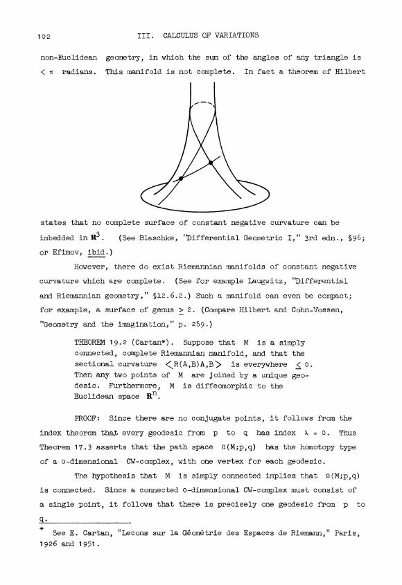
102 III. CALCULUS OF VARIATIONS
non-Euclidean geometry, in which the sum of the angles of any triangle is
< it radians. This manifold is not complete. In fact a theorem of Hilbert
states that no complete surface of constant negative curvature can be
imbedded in R3. (See Blaschke, "Differential Geometric I," 3rd edn., §96;
or Efimov, ibid.)
However, there do exist Riemannian manifolds of constant negative
curvature which are complete. (See for example Laugwitz, "Differential
and Riemannian geometry," §12.6.2.) Such a manifold can even be compact;
for example, a surface of genus > 2. (Compare Hilbert and Cohn-Vossen,
"Geometry and the imagination," p. 259.)
THEOREM 19.2 (Cartan*). Suppose that M is a simply
connected, complete Riemannian manifold, and that the
sectional curvature KR(A,B)A,B > is everywhere < 0.
Then any two points of M are joined by a unique geo-
desic. Furthermore, M is diffeomorphic to the
Euclidean space Rn.
PROOF: Since there are no conjugate points, it follows from the
index theorem that every geodesic from p to q has index X = 0. Thus
Theorem 17.3 asserts that the path space 0(M;p,q) has the homotopy type
of a 0-dimensional CW-complex, with one vertex for each geodesic.
The hypothesis that M is simply connected implies that Q(M;p,q)
is connected. Since a connected 0-dimensional CW-complex must consist of
a single point, it follows that there is precisely one geodesic from p to
q.*
See E. Cartan, "Lecons sur la Geometrie des Espaces de Riemann," Paris,
1926 and 1951.

§19. TOPOLOGY AND CURVATURE 103
Therefore, the exponential map expp: TMp - M is one-one and
onto. But it follows from 18.1 that expp is non-critical everywhere;
so that expp is locally a diffeomorphism. Combining these two facts, we
see that expp is a global diffeomorphism. This completes the proof of
19.2.
More generally, suppose that M is not simply connected; but is
complete and has sectional curvature < 0. (For example M might be a
flat torus S1 X S1, or a compact surface of genus > 2 with constant
negative curvature.) Then Theorem 19.2 applies to the, universal coveringti
space M of M. For it is clear that M inherits a Riemannian metric
from M which is geodesically complete, and has sectional curvature < 0.
Given two points p,q E M, it follows that each homotopy class of
paths from p to q contains precisely one geodesic.
The fact that M is contractible puts strong restrictions on the
topology of M. For example:
COROLLARY 19.3. If M is complete with <R(A,B)A,B
< 0 then the homotopy groups ai(M) are zero for
i > 1; and a1(M) contains no element of finite order
other than the identity.
PROOF: Clearly ai(M) = j(M) = 0 for i > 1. Since M is
contractible the cohomology group 11k(M) can be identified with the co-
homology group Hk(a1(M)) of the group a1(M). (See for example pp. 200-
202 of S. T. Hu "Homotopy Theory," Academic Press, 1959.) Now suppose
that a1(M) contains a non-trivial finite cyclic subgroup G. Then for a
suitable covering space M of M we have a1(M) = G; hence
Hk(G) = Hk(M) = 0 for k > n .
But the cohomology groups of a finite cyclic group are non-trivial in arbi-
trarily high dimensions. This gives a contradiction; and completes the
proof.Now we will consider manifolds with "positive curvature." Instead
of considering the sectional curvature, one can obtain sharper results in
this case by considering the Ricci tensor (sometines called the "mean curva-
ture tensor").

io4 III. CALCULUS OF VARIATIONS
DEFINITION. The Ricci tensor at a point p of a Riemannian mani-
fold M is a bilinear pairing
K: TMp x TMp R
defined as follows. Let K(U1,U2) be the trace of the linear transforma-
tion
W R(U1,W)U2
from TMp to TMp. (In classical terminology the tensor K is obtained
from R by contraction.) It follows easily from §9.3 that K is symmetric:
K(U1,U2) = K(U2,U1).
The Ricci tensor is related to sectional curvature as follows. Let
U1,U2,...,Un be an orthonormal basis for the tangent space TMp.
ASSERTION. K(Un,Un) is equal to the sum of the sectional curva-
tures < R(Un,Ui)Un,Ui > for i = 1,2,...,n-1.
PROOF: By definition K(Un,Un) is equal to the trace of the matrix
( K R(Un,Ui)Un,Uj > ) . Since the n-th diagonal term of this matrix is
zero, we obtain a sum of n-1 sectional curvatures, as asserted.
THEOREM 19.4 (Myers*). Suppose that the Ricci curvature
K satisfies
K(U,U) > (n-1)/r2
for every unit vector U at every point of M; where r
is a positive constant. Then every geodesic on M of
length > Ar contains conjugate points; and hence is not
minimal.
PROOF: Let y: [0,11 - M be a geodesic of length L. Choose
parallel vector fields P1,...,Pn along y which are orthonormal at one
point, and hence are orthonormal everywhere along y. We may assume that
Pn points along y, so that
DPV = = L Pn , and i
Let Wi(t) _ (sin at) Pi(t). Then
= 0
See S. B. Myers, Riemann manifolds with positive mean curvature, Duke
Math. Journal, Vol. 8 (1941), pp. 4o1-404.

§19. TOPOLOGY AND CURVATURE
1 D2W.
2E**i,Wi) _ - $ < Wi, dt2 + R(V,Wi)V > dt
0
105
1
S(sin at)2
(a2- L2 < R(Pn,PI)Pn,Pi > ) dt.
0
Summing for i = 1,...,n-1 we obtain
1 7- )> dt2 L2 K(P P)t 2 ic - n((n-1 n,(sin n )
0
Now if K(Pn,Pn) > (n-1)/r2 and L > ar then this expression is
< o. Hence E**(Wi,Wi) < 0 for some i. This implies that the index of
y is positive, and hence, by the Index Theorem, that y contains conju-
gate points.
It follows also that y is not a minimal geodesic. In fact if
a is a variation with variation vector field Wi then
dE(a(u))=- d2E(a(u))
CTU_
0,
du2
< o
for u = 0. Hence E(a(u)) < E(y) for small values of u # 0. This com-
pletes the proof.
EXAMPLE. If M is a sphere of radius r then every sectional
curvature is equal to 1/r2. Hence K(U,U) takes the constant value
(n-1)/r2. It follows from 19.4 that every geodesic of length > ar con-
tains conjugate points: a best possible result.
COROLLARY 19.5. If M is complete, and K(U,U) >
(n-1) /r2 > o for all unit vectors U, then M is
compact, with diameter < ar.
PROOF. If p,q e M let y be a minimal geodesic from p to q.
Then the length of y must be < ar. Therefore, all points have distance
< ar. Since closed bounded sets in a complete manifold are compact, it
follows that M itself is compact.
This corollary applies also to the universal covering space M of
M. Since M is compact, it follows that the fundamental group a1(M) is
finite. This assertion can be sharpened as follows.
106 III. CALCULUS OF VARIATIONS
THEOREM 19.6. If M is a compact manifold, and if the
Ricci tensor K of M is everywhere positive definite,
then the path space 11(M;p,q) has the homotopy type of
a CW-complex having only finitely many cells in each
dimension.
PROOF. Since the space consisting of all unit vectors U on M
is compact, it follows that the continuous function K(U,U) > 0 takes on
a minimum, which we can denote by (n-1)/r2 > 0. Then every geodesic
y E 0(M;p,q) of length > ar has index X > 1.
More generally consider a geodesic y of length > kirr. Then a
similar argument shows that y has index >v > k. In fact for each
i = 1,2,...,k one can construct a vector field Xi along y which vanishes
i-1 ioutside of the interval ( ,
k), and such that E**(Xi,Xi) < 0.
Clearly E**(Xi,Xi ) = 0 for i j; so that X1,...,Xk span a k -
dimensional subspace of TOy on which E** is negative definite.
Now suppose that the points p and q are not conjugate along any
geodesic. Then according to § 16.3 there are only finitely many geodesics
from p to q of length < ksr. Hence there are only finitely many geo-
desics with index < k. Together with §17.3, this completes the proof.
REMARK. I do not know whether or not this theorem remains true if
M is allowed to be complete, but non-compact. The present proof certainly
breaks down since, on a manifold such as the paraboloid z = x2 + y2, the
curvature K(U,U) will not be bounded away from zero.
It would be interesting to know which manifolds can carry a metric
so that all sectional curvatures are positive. An instructive example is
provided by the product Sm X Sk of two spheres; with m,k > 2. For this
manifold the Ricci tensor is everywhere positive definite. However, the
sectional curvatures in certain directions (corresponding to flat tori
S1 X S1 C Sm X Sk) are zero'. It is not known whether or not Sm x Sk can
be remetrized so that all sectional curvatures are positive. The following
partial result is known: If such a new metric exists, then it can not be
invariant under the involution (x,y) -+ (-x,-y) of Sm x Sk. This follows
from a theorem of Synge. (See J. L. Synge, On the connectivity of spaces
§19. TOPOLOGY AND CURVATURE 107
of positive curvature, Quarterly Journal of Mathematics (Oxford), Vol. 7
(1936), pp. 316-320.
For other theorems relating topology and curvature, the following
sources are useful.
K. Yano and S. Bochner, "Curvature and Betti Numbers," Annals
Studies, No 32, Princeton, 1953.
S. S. Chern, On curvature and characteristic classes of a Riemann
manifold, Abh. Math. Sem., Hamburg, Vol. 20 (1955), pp. 117-126.
M. Berger, Sur certaines varietes Riemanniennes a courbure positive,
Comptes Rendus Acad. Sci., Paris, Vol. 247 (1958), pp. 1165-1168.
S. I. Goldberg, "Curvature and Homology," Academic Press, 1962.


109
PART IV.
APPLICATIONS TO LIE GROUPS AND SYMMETRIC SPACES
§20. Symmetric Spaces.
A symmetric space is a connected Riemannian manifold M such that,
for each p e M there is an isometry Ip
: M M which leaves p fixed
and reverses geodesics through p, i.e., if y is a geodesic and y(0) = p
then Ip(y(t)) = y(-t).
LEMMA 20.1 Let y be a geodesic in M, and let
p = y(o) and q = y(c). Then IgIp(y(t)) = y(t + 2c)
(assuming y(t) and y(t + 2c) are defined). More-
over, Iqlp preserves parallel vector fields along y
PROOF: Let y'(t) = y(t + c). Then y' is a geodesic and
y'(o) = q. Therefore IgIp(y(t)) = Iq(y(-t)) = Iq(y'(-t - c)) =
y'(t + c) = y(t + 2c).
If the vector field V is parallel along y then Ip*(V) is
parallel (since Ip is an isometry) and Ip*V(o) = -V(o); therefore
Ip*V(t) = -V(-t). Therefore Iq* Ip*(V(t)) = V(t + 2c).
COROLLARY 20.2. M is complete.
Since 20.1 shows that geodesics can be indefinitely extended.
COROLLARY 20.3. 1P is unique.
Since any point is joined to p by a geodesic.
COROLLARY 20.4. If U,V and W are parallel vectorfields along y then R(U,V)W is also a parallel
field along y.
PROOF. If X denotes a fourth parallel vector field along y,
note that the quantity < R(U,V)W,X > is constant along y. In fact,
110 IV. APPLICATIONS
given p = y(o), q = y(c), consider the isometry T = Iy(c/2)Ip which
carries p to q. Then
<R(Uq,Vq)Wq,Xq> = < R(T*UU,T*VV)T. WW,T. Xp>
by 20.1. Since T is an isometry, this quantity is equal to
< R(UJ,VV)WW,Xp> . Thus <R(U,V)W,X> is constant for every parallel
vector field X. It clearly follows that R(U,V)W is parallel.
Manifolds with the property of 20.4 are called locally symmetric.
(A classical theorem, due to Cartan states that a complete, simply connected,
locally symmetric manifold is actually symmetric.)
In any locally symmetric manifold the Jacobi differential equations
have simple explicit solutions. Let y: R - M be a geodesic in a local-
ly symmetric manifold. Let V = mo(o) be the velocity vector at p = y(o).
Define a linear transformation
TM__KV: TMp -+ TM
by KV(W) = R(V,W)V. Let el,...,en denote the eigenvalues of Kv.
THEOREM 20.5. The conjugate points to p along y
are the points y(ak/e) where k is any non-zero
integer, and ei is any positive eigenvalue of KV.
The multiplicity of y(t) as a conjugate point is
equal to the number of ei such that t is a mul-
tiple of n/ e .
PROOF: First observe that KV is self-adjoint:
KV(W),W'> = <W,Kv(W')
This follows immediately from the symmetry relation
R(V,W)V',W' > = KR(V',W')V,W
Therefore we may choose an orthonormal basis U1, ...,Un for Mp so that
Kv.(Ui) = eiUi ,
where e1, ... ,en are the eigenvalues. Extend the Ui to vector fields
along y by parallel translation. Then since M is locally symmetric,
KV should not be confused with the Ricci tensor of §19.
520. SYMMETRIC SPACES 111
the condition
R(V,Ui)V = eiUi
remains true everywhere along y. Any vector field W along y may be
expressed uniquely as
W(t) = w1(t)U1(t) +...+ wn(t)Un(t) .
2
Then the Jacobi equation + KV(W) = 0 takes the formTt
d2w
L dt2 Ui + eiwiUi = 0.
Since the Ui are everywhere linearly independent this is equivalent to
the system of n equations
d2wi
et+ eiw1 0
We are interested in solutions that vanish at t = 0. If ei > 0 then
wi(t) = ci sin (f t), for some constant ci.
Then the zeros of wi(t) are at the multiples of t = n/qre-i
If ei = o then wi(t) = cit and if ei < 0 then
wi(t) = ci sinh (41 for some constant ci. Thus if ei < 0, wi(t)
vanishes only at t = 0. This completes the proof of 20.5.
112 IV. APPLICATIONS
§21. Lie Groups as Symmetric Spaces.
In this section we consider a Lie group G with a Riemannian metric
which is invariant both under left translations
LT: G -* G, LT(a) = T a
and right translation, RT(a) = aT. If G is commutative such a metric
certainly exists. If G is compact then such a metric can be constructed
as follows: Let <> be any Riemannian metric on G, and Let .t denote
the Haar measure on G. Then .t is right and left invariant. Define a
new inner product <<, >> on G by
<< V,W >> = S < La*RT*(V), La*RT*(W) > du(a) du(T)
GxG
Then <<,>> is left and right invariant.
LEMMA 21.1 If G is a Lie group with a left and right
invariant metric, then G is a symmetric space. The
reflection IT in any point T E G is given by the
formula IT(a) = Ta-1 T.
PROOF: By hypothesis LT and RT are isometries. Define a map
Ie: G G by
Ie(a) =
Then Ie*: TGe TGe reverses the tangent space of e; so is certainly
an isometry on this tangent space. Now the identity
Ie = R1IeLa_1
shows that Ie*: TGa --) TGa-1 is an isometry for any a E G. Since Ie
reverses the tangent space at e, it reverses geodesics through e.
Finally, defining IT(a) = Ta-1T, the identity I. = RTIeRT1
shows that each IT is an isonetry which reverses geodesics through T.
A 1-parameter subgroup of G is a C°° homomorphism of R into
G. It is well known that a 1-parameter subgroup of G is determined by
its tangent vector at e. (Compare Chevalley, "Theory of Lie Groups,"
Princeton, 1946.)

§21. LIE GROUPS 113
LEMMA 21.2. The geodesics y in G with y(O) = e
are precisely the one-parameter subgroups of G.
PROOF: Let y: R - G be a geodesic with y(o) = e. By Lemma 20.1
the map Iy(t)Ie takes y(u) into y(u + 2t). Now Iv(t)Ie(a) = y(t)a y(t)
so y(t)y(u)y(t) = y(u + 2t). By induction it follows that y(nt) = y(t)n
for any integer n. If t'/t" is rational so that t' = nit and t" = n"t"
for some t and some integers n' and n" then y(t' + t") = y(t)n +n =
y(t')y(t"). By continuity y is a hor..omorphism.
Now let y: R G be a 1-parameter subgroup. Let y' be the
geodesic through e such that the tangent vector of y' at e is the tan-
gent vector of y at e. We have just seen that 7 is a 1-parameter sub-
group. Hence y' = y. This completes the proof.
A vector field X on a Lie group G is called left invariant if
and only if (La)*(Xb) = Xa,b for every a and b in G. If X and Y
are left invariant then [X,Y] is also. The Lie algebra g of G is the
vector space of all left invariant vector fields, made into an algebra by
the bracket [ 1.
g is actually a Lie algebra because the Jacobi identity
[[x,Y],Z] + [[Y,Z],x] + [[Z,X],Y] = 0
holds for all (not necessarily left invariant) vector fields X,Y and Z.
THEOREM 21.3. Let G be a Lie group with a left and
right invariant Riemannian metric. If X,Y,Z and Ware left invariant vector fields on G then:
a) <[X,YI,Z> = <X,[Y,ZI>b) R(X,Y)Z = - [[X,Y],ZIc) < R(X,Y)Z,W > < [X,YI,[Z,W1 >
PROOF: As in §8 we will use the notation X F Y for the covariant
derivative of Y in the direction X. For any left invariant X the iden-
tity
x FX = 0
is satisfied, since the integral curves of X are left translates of 1-
parameter subgroups, and therefore are geodesics.

114 IV. APPLICATIONS
Therefore
is zero; hence
On the other hand
(X + Y) F (X + Y) = (X F X) + (X F Y)
+ (Y F X) + (Y F Y)
X F Y+ Y F X = 0.
X FY -Y FX = [X,Y]
by §8.5. Adding these two equations we obtain:
d) 2X F Y = [X,Y]
Now recall the identity
Y (X,Z> = <Y F X,Z> + <X,Y F Z > .
(See §8.4.) The left side of this equation is zero, since <X,Z > is
constant. Substituting formula (d) in this equation we obtain
0 = < [Y,X] , Z> + <X, [Y, Z] > .
Finally, using the skew commutativity of [Y,X], we obtain the required
formula
(a) <[X,Y],Z> _ <X,[Y,Z]>
By definition, R(X,Y)Z is equal to
- X F (Y F Z) + Y F (X F Z) + [X,Y] F Z.
Substituting formula (d), this becomes
- -[X,[Y,Z]] + -[Y,[X,Z]] + 2[[X,Y],Z]
Using the Jacobi identity, this yields the required formula
(b) R(X,Y)Z = 7[[X,Y],Z] .
The formula (c) follows from (a) and (b) .
It follows that the tri-linear function X,Y,Z -+ <IX,Y],Z > is skew-
symmetric in all three variables. Thus one obtains a left invariant differ-
ential 3-form on G, representing an element of the de Rham cohomology group
H3(G). In this way Cartan was able to prove that H3(G) # 0 if G is a
non-abelian compact connected Lie group. (See E. Cartan, "La Topologie des
Espaces Representatives des Groupes de Lie," Paris, Hermann, 1936.)
§21. LIE GROUPS 115
COROLLARY 21.4. The sectional curvature < R(X,Y)X,Y
K [X,Y],[X,Y] > is always > 0. Equality holds if and
only if [X,Y] = 0.
Recall that the center c of a Lie algebra g is defined to be
the set of X E g such that [X,Y] = 0 for all Y E g.
COROLLARY 21.5. If G has a left and right invariant
metric, and if the Lie algebra g has trivial center,
then G is compact, with finite fundamental group.
PROOF: This follows from Meyer's theorem (§19). Let X1 be any
unit vector in g and extend to a orthonormal basis X1,...,Xn. The Ricci
curvature
K(X1,X1) _ 2. (R(X1,Xi)X1,Xii=1
must be strictly positive, since [X1,Xi) / 0 for some i. Furthermore
K(X1,X1) is bounded away from zero, since the unit sphere in g is compact.
Therefore, by Corollary 19.5, the manifold G is compact.
This result can be sharpened slightly as follows.
COROLLARY 21.6. A simply connected Lie group G with left
and right invariant metric splits as a Cartesian product
G' x Rk where G' is compact and Rk denotes the additive
Lie group of some Euclidean space. Furthermore, the Lie
algebra of G' has trivial -center.
Conversely it is clear that any such product G' x Rk possesses a
left and right invariant metric.
PROOF. Let c be the center of the Lie algebra g and let
g' _ (X E g : <X, C> = 0 for all C E c )
be the orthogonal complement of c. Then g' is a Lie sub-algebra. For
if X,Y E g' and C E c then
[X,Y],C > = <X, 1Y,C1 > = o;
hence [X,Y] E g'. It follows that g splits as a direct sum g' ® C of
Lie algebras. Hence G splits as a Cartesian product G' x G"; where G'
is compact by 21.5 and G" is simply connected and abelian, hence isomorphic
116 TV. APPLICATIONS
to some Rk. (See Chevalley, "Theory of Lie Groups.") This completes the
proof.
THEOREM 21.7 (Bott). Let G be a compact, simply con-
nected Lie group. Then the loop space 0(G) has the
homotopy type of a CW-complex with no odd dimensional
cells, and with only finitely many X-cells for each
even value of X.
Thus the x-th homology groups of 01(G) is zero for . odd, and is
free abelian of finite rank for a. even.
REMARK 1. This CW-complex will always be infinite dimensional. As
an example, if G is the group S3 of unit quaternions, then we have seen
that the homology group Hi01(S3) is infinite cyclic fqr all even values of i.
REMARK 2. This theorem remains true even for a non-compact group.
In fact any connected Lie group contains a compact subgroup as deformation
retract. (See K. Iwasawa, On some types of topological groups, Annals of
Mathematics 50 (1949), Theorem 6.)
PROOF of 21.7. Choose two points p and q in G which are not
conjugate along any geodesic. By Theorem 17.3, Q(G;p,q) has the homotopy
type of a CW-complex with one cell of dimension X for each geodesic from
p to q of index X. By §19.4 there are only finitely many %-cells for
each X. Thus it only remains to prove that the index X of a geodesic is
always even.
Consider a geodesic y starting at p with velocity vector
V = mo(o) e TGp = g .
According to §20.5 the conjugate points of p on y are determined by the
eigenvalues of the linear transformation
KV : TGp - TGp ,
defined by
KV(W) = R(V,W)V = 7[[V,w],V]
Defining the adjoint homomorphism
Ad V: S1 9
§21. LIE GROUPS 117
by
we have
Ad V(W) _ [V,W]
KV = - - (Ad V) o (Ad V)
The linear transformation Ad V is skew-symmetric; that is
Ad V(W),W' > _ - < W,Ad V(W') > .
This follows immediately from the identity 21.3a. Therefore we can choose
an orthonormal basis for (4 so that the matrix of Ad V takes the form
-a2
It follows that the composite linear transformation (Ad V)o(Ad V) has
matrix
0 a2
2 2
a2
Therefore the non-zero eigenvalues of KV - --(Ad V)2 are positive, and
occur in pairs.
It follows from 20.5 that the conjugate points of p along y also
occur in pairs. In other words every conjugate point has even multiplicity.
Together with the Index Theorem, this implies that the index ? of any
geodesic from p to q is even. This completes the proof.
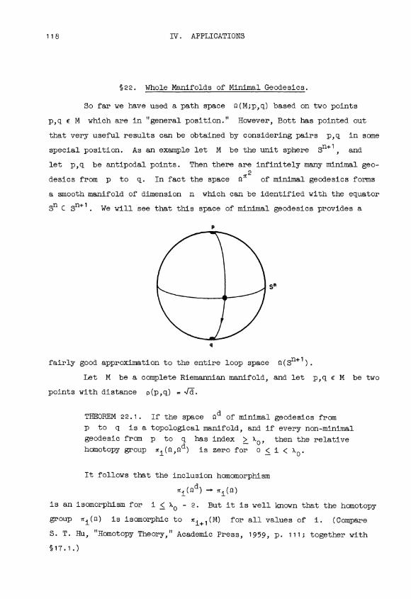
118 IV. APPLICATIONS
§22. Whole Manifolds of Minimal Geodesics.
So far we have used a path space o(M;p,q) based on two points
p,q c M which are in "general position." However, Bott has pointed out
that very useful results can be obtained by considering pairs p,q in some
special position. As an example let M be the unit sphere Sn+1,
and
let p,q be antipodal points. Then there are infinitely many minimal geo-
desics from p to q. In fact the space saa of minimal geodesics forms
a smooth manifold of dimension n which can be identified with the equator
Sn C Sn+1. We will see that this space of minimal geodesics provides a
fairly good approximation to the entire loop space 0(Sn+1)
Let M be a complete Riemannian manifold, and let p,q c M be two
points with distance p(p,q) =-,r-d.
THEOREM 22.1. If the space Std of minimal geodesics from
p to q is a topological manifold, and if every non-minimal
geodesic from p to q has index > Xo, then the relative
homotopy group ai(o,Std) is zero for 0 < i < X0.
It follows that the inclusion homomorphism
ai(rid - ai(a)is an isomorphism for i < Xo - 2. But it is well known that the homotopy
group ai(Sc) is isomorphic to ai+1(M) for all values of i. (Compare
S. T. Hu, "Homotopy Theory," Academic Press, 1959, p. 111; together with
§17.1.)

§22. MANIFOLDS OF MINIMAL GEODESICS 119
Thus we obtain:
COROLLARY 22.2. With the same hypotheses, ei(od) is
isomorphic to a1+1(M) for 0 < i < Xo - 2.
Let us apply this corollary to the case of two antipodal points on
the (n+1)-sphere. Evidently the hypotheses are satisfied with 1`0 = 2n.
For any non-minimal geodesic must wind one and a half times aroundSn+1;
and contain two conjugate points, each of multiplicity n, in its interior.
This proves the following.
COROLLARY 22.3. (The Freudenthal suspension theorem.)
The homotopy group ,ri(Sn) is isomorphic to"i+1(Sn+1)
for i < 2n-2.
Theorem 22.1 also implies that the homology groups of the loop
space 0 are isomorphic to those of S;d in dimensions < %0 - 2. This
fact follows from 22.1 together with the relative Hurewicz theorem. (See
for example Hu, p. 306. Compare also J. H. C. Whitehead, Combinatorial
homotopy I, Theorem 2.)
The rest of §22 will be devoted to the proof of Theorem 22.1. The
proof will be based on the following lemma, which asserts that the condition
"all critical points have index > %o" remains true when a function is
jiggled slightly.
Let K be a compact subset of the Euclidean space Rn; let U be
a neighborhood of K; and let
f: U R
be a smooth function such that all critical points of f in K have index
)o.
LEMMA 22.4. If g: U R is any smooth function which
is "close" to f, in the sense that
la_ of I
<3xi '3i E a2g _ a2fxT 8x c)xi
uniformly throughout K, for some sufficiently small constant s
then all critical points of g in K have index > Xo.
,
(Note that f is allowed to have degenerate critical points. In
the application, g will be a nearby function without degenerate critical
points.)
120 IV. APPLICATIONS
PROOF of 22.4. The first derivatives of g are roughly described
by the single real valued function
kg(x)= mo f
> o1
on U; which vanishes precisely at the critical points of g. The second
derivatives of g can be roughly described by n continuous functions
eg,..., eg: U - R
as follows. Let
e11(x) < e2(x) <... < eg(x)9 9
2denote the n eigenvalues of the matrix ( x ) . Thus a critical point
x of g has index > ? if and only if the number eg(x) is negative.
The continuity of the functions eg follows from the fact that the
X-th eigenvalue of a symmetric matrix depends continuously on the matrix*.
This can be proved, for example, using the fact that the roots of a complex
polynomial of degree n vary continuously with the coefficient of the poly-
nomial. (Rouche's theorem.)
Let mg(x) denote the larger of the two numbers kg(x) and -e g W.
Similarly let mf(x) denote the larger of the corresponding numbers kf(x)
and -ef (x). The hypothesis that all critical points of f in K have
index > X0 implies that -ef (x) > 0 whenever kf(x) = 0. In other words
mf(x) > 0 for all x E K.
Let s > 0 denote the minimum of mf on K. Now suppose that g
is so close to f that
(*) kg(x) - kf(x) I < e, leg (x) - of (x)I < e
for all x E K. Then mg(x) will be positive for x E K; hence every
critical point of g in K will have index > X0.
This statement can be sharpened as follows. Consider two nxn symmetric
matrices. If corresponding entries of the two matrices differ by at most
e, then corresponding eigenvalues differ by at most ne. This can be
proved using Courant's minimax definition of the X-th eigenvalue. (See
§1 of Courant, Uber die Abhangigkeit der Schwingungszahlen einer Membran...,
Nachrichten, Kbniglichen Gesellschaft der Wissenschaften zu Gottingen, Math.
Phys. Klasse 1919, pp. 255-264.)

§22. MANIFOLDS OF MINIMAL GEODESICS 121
To complete the proof of 22.4, it is only necessary to show that
the inequalities (*) will be satisfied providing that
g 2g 2`zi - 4i l < E and I xcc1 x x1c 6x < E
for sufficiently small a. This follows by a uniform continuity argument
which will be left to the reader (or by the footnote above ).
We will next prove an analogue of Theorem 22.1 for real valued
functions on a manifold.
Let f: M -+ R be a smooth real valued function with minimum o,
such that each Me = f-1[o,c] is compact.
LEMMA 22.5. If the set M0 of minimal points is a manifold,
and if every critical point in M - M0 has index > Xo,
then ar(M,M°) = 0 for 0 < r < X0.
PROOF: First observe that Mo is a retract of some neighborhood
U C M. In fact Hanner has proved that any manifold M0 is an absolute
neighborhood retract. (See Theorem 3.3 of 0. Hanner, Some theorems on
absolute neighborhood retracts, Arkiv for Matematik, Vol. 1 (1950), pp.
389-408.) Replacing U by a smaller neighborhood if necessary, we may
assume that each point of U is joined to the corresponding point of M0
by a unique minimal geodesic. Thus U can be deformed into Mo within M.
Let Ir denote the unit cube of dimension r < Xp, and let
h: (Ir,Ir) _ (M,MO)
be any map. We must show that h is homotopic to a map h' with
h'(Ir) C Mo.
Let c be the maximum of f on h(Ir). Let 35 > 0 be the mini-
mum of f on the set M - U. (The function f has a minimum on M - U
since each subset Mc - U is compact.)
Now choose a smooth function
g:Mc+2s R
which approximates f closely, but has no degenerate critical points. This
is possible by §6.8. To be more precise the approximation should be so
close that:
(1) Jf(x) - g(x)l < s for all x E Mc+2s. and

122 IV. APPLICATIONS
(2) The index of g at each critical point which lies in the com-
pact set f-1[8,c+28] is > x0.
It follows from Lemma 22.4 that any g which approximates f
sufficiently closely, the first and second derivatives also being approxi-
mated, will satisfy (2). In fact the compact set f-'[8,0+281 can be
covered by finitely many compact set Ki, each of which lies in a coordi-
nate neighborhood. Lemma 22.4 can then be applied to each Ki.
The proof of 22.5 now proceeds as follows. The function g is
smooth on the compact region g 1[25,c+s] C f 1[s,c+2sl, and all critical
points are non-degenerate, with index > ).0. Ience the manifold
g-1
(--,c+bl has the homotopy type of g 1(-oo,2s] with cells of dimension
> X0 attached.
Now consider the map
h:Ir jr Mc,MO
C g 1(-oo,c+s],MO
Since r < X0
it follows that h is homotopic within g1(-oo,c+s],M0 to
a map
h': Ir,Ir -y g-1 (--22812M 0 .
But this last pair is contained in (U,MO); and U can be deformed into
MO within M. It follows that h' is homotopic within (M,MO) to a map
h": Ir,Ir - MO,M0. This completes the proof of 22.5.
The original theorem, 22.1, now can be proved as follows. Clearly
it is sufficient to prove that
si(Int 0c,fd) = o
for arbitrarily large values of c. As in §16 the space Int 0c contains
a smooth manifold Int ac(to,t1,...,tk) as deformation retract. The space
sad of minimal geodesics is contained in this smooth manifold.
The energy function E: a --' R, when restricted to
Int sac(t0,t1,...,tk), almost satisfies the hypothesis of 22.5. The only
difficulty is that E(m) ranges over the interval d < E < c, instead of
the required interval [o,oo). To correct this, let
F. [d,c) - [o,o)
be any diffeomorphism.
§22. MANIFOLDS OF MINIMAL GEODESICS 123
Then
F ° E: Int oc(tc,t1,...,tk) R
satisfies the hypothesis of 22.5. Hence
si(Int cc(tp,...,tk),12d) = ni(Int fc,0d)
is zero for i < Xc. This completes the proof.
124 IV. APPLICATIONS
§23. The Bott Periodicity Theorem for the Unitary Group.
First a review of well known facts concerning the unitary group.
Let C n be the space of n-tuples of complex numbers, with the usual Her-
mitian inner product. The unitary group U(n) is defined to be the group
of all linear transformationsS. Cn -Cn which preserve this inner
product. Equivalently, using the matrix representation, U(n) is the
group of all n x n complex matrices S such that S S* = I; where S*
denotes the conjugate transpose of S.
For any n x n complex matrix A the exponential of A is defined
by the convergent power series expansion
exp A = I+A+ 1 A2+1A3 + ...
The following properties are easily verified:
(1) exp (A*) = (exp A)*; exp (TAT-1) = T(exp A)T-1.
(2) If A and B commute then
exp (A + B) _ (exp A)(exp B). In particular:
(3) (exp A)(exp -A) = I
(4) The function exp maps a neighborhood of 0 in the space of
n x n matrices diffeomorphically onto a neighborhood of I.
If A is skew-Hermitian (that is if A + A* = 0), then it fol-
lows from (1) and (3) that exp A is unitary. Conversely if exp A is
unitary, and A belongs to a sufficiently small neighborhood of 0, then
it follows from (1), (3), and (4) that A + A* = 0. From these facts one
easily proves that:
(5) U(n) is a smooth submanifold of the space of n x n matrices;
(6) the tangent space TU(n)I can be identified with the space of
n x n skew-Hermitian matrices.
Therefore the Lie algebra g of U(n) can also be identified with
the space of skew-Hermitian matrices. For any tangent vector at I extends
uniquely to a left invariant vector field on U(n). Computation shows that
the bracket product of left invariant vector fields corresponds to the
product [A,B] = AB - BA of matrices.
§23. THE BOTT PERIODICITY THEOREM 125
Since U(n) is compact, it possesses a left and right invariant
Riemannian metric. Note that the function
exp: TU(n) I - U(n)
defined by exponentiation of matrices coincides with the function exp de-
fined (as in §10) by following geodesics on the resulting Riemannian mani-
fold. In fact for each skew-Hermitian matrix A the correspondence
t - exp(t A)
defines a 1-parameter subgroup of U(n) (by Assertion (2) above); and
hence defines a geodesic.
A specific Riemannian metric on U(n) can be defined as follows.
Given matrices A,B e g let <A,B > denote the real part of the complex
number
trace (AB*) = Aij$ij .
1,3
Clearly this inner product is positive definite on g .
This inner product on g determines a unique left invariant
Riemannian metric on U(n). To verify that the resulting metric is also
right invariant, we must check that it is invariant under the adjoint
action of U(n) on g .
DEFINITION of the adjoint action. Each S E U(n) determines an
inner automorphism
X - S X S-1= (LSRS-1 )X
of the group U(n). The induced linear mapping
(LSRS-1)*: TU(n)I --. TU(n)I
is called Ad(S). Thus Ad(s) is an automorphism of the Lie algebra of
U(n). Using Assertion (1) above we obtain the explicit formula
Ad(S)A = SAS 1 ,
for A E g, S E U(n).
The inner product <A,B> is invariant under each such automorphism
Ad(S). In fact if Al = Ad(S)A, B1 = Ad(S)B then the identity
A1B1*= SAS-1(SBS 1)* =
SAB*S-1

126 1V. APPLICATIONS
implies that
trace (A1B1*) = trace (SAB*S 1) = trace (AB*) ;
and hence that
KA1,B1 > = < A,B
It follows that the corresponding left invariant metric on U(n) is also
right invariant.
Given A c g we know by ordinary matrix theory that there exists
T E U(n) so that TAT 1 is in diagonal form
TAT-1
=
ia2
where the ails are real. Also, given any S E U(n), there is a T E U(n)
such that
TST-1
=ian
e
where again the ails are real. Thus we see directly that exp: g -iJ(n)
is onto.
One may treat the special unitary group SU(n) in the same way.
SU(n) is defined as the subgroup of U(n) consisting of matrices of de-
terminant 1. If exp is regarded as the ordinary exponential map of
matrices, it is easy to show, using the diagonal form, that
det (exp A) = etrace A
Using this equation, one may show that g' , the Lie algebra of SU(n) is
the set of all matrices A such that A + A* = 0 and trace A = 0.
In order to apply Morse theory to the topology of U(n) and SU(n),
we begin by considering the set of all geodesics in U(n) from I to -I.
In other words, we look for all A E TU(n)1 = g such that exp A = -I.
Suppose A is such a matrix; if it is not already in diagonal form, let
T E U(n) be such that TAT-1
is in diagonal form. Then
exp TAT-1 = T(exp A)T-1
= T(-I)T-1 = -I

§23. THE BOTT PERIODICITY THEOREM 127
so that we may as well assume that A is already in diagonal form
/ ia1
1e
iane
so that exp A = -I if and only if A has the form
/ k1 inI
k2in.
for some odd integers k1,...,kn.
Since the length of the geodesic t -+ exp to from t = 0 to t = 1
is JAI = tJ r AA*, the length of the geodesic determined by A is
it k'1 +...+ kn. Thus A determines a minimal geodesic if and only if each
ki equals + 1, and in that case, the length is n f-n. Now, regarding
such an A as a linear map of Cn to Cn observe that A is completely
determined by specifying Eigen(in), the vector space consisting of all
v E Cn such that Av = inv; and Eigen(-in), the space of all v E Cn
such that Av = -inv. Since Cn splits as the orthogonal sum Eigen(in)
Eigen(-in), the matrix A is then completely determined by Eigen(in),
which is an arbitrary subspace of Cn. Thus the space of all minimal geo-
desics in U(n) from I to -I may be identified with the space of all
sub-vector -spaces of C
Unfortunately, this space is rather inconvenient to use since it
has components of varying dimensions. This difficulty may be removed by
replacing U(n) by SU(n) and setting n = 2m. In this case, all the
above considerations remain valid. But the additional condition that
a1 +...+ a2m = 0 with ai = + n restricts Eigen(in) to being an arbi-
trary m dimensional sub-vector-space of C. This proves the following:2m
/ is

128 IV. APPLICATIONS
LEMMA 23.1. The space of minimal geodesics from I to -I
in the special unitary group SU(2m) is homeomorphic to the
complex Grassmann manifold Gm(C2m), consisting of all m
dimensional vector subspaces ofC2m.
We will prove the following result at the end of this section.
LEMMA 23.2. Every non-minimal geodesic from I to -I
in SU(2m) has index > 2m+2.
Combining these two lemmas with §22 we obtain:
THEOREM 23.3 (Bott). The inclusion map Gm(CM) _
ci(SU(2m); 1,-I) induces isomorphisms of homotopy groups
in dimensions < 2m. Hence
tti Gm(CSm) - tti+1SU(2m)
for i<2m.
On the other hand using standard methods of homotopy theory one
obtains somewhat different isomorphisms.
LEMMA 23.4. The group ttiGm(C2m) is isomorphic to
tti-t U(m) for i < 2m. Furthermore,
U(m) = I(i-1
U(m+1) = I(i-1
U(m+2) = ..
for i < 2m; and
for j X 1.ttj U(m) = ttj SU(m)
PROOF. First note that for each m there exists a fibration
U(m) - U(m+1)-wS2m+1
From the homotopy exact sequence
-F tti 2m+1 2m+1g xi-1 U(m) -if,-, U(m+1) -1(i-1 S ...of this fibration we see that
tti-1 U(m) - tti_1 U(m+t) for i < 2m.
(Compare Steenrod, "The Topology of Fibre Bundles," Princeton, 1951, p. 35
and p. 9o.) It follows that the inclusion homomorphisms
tti-1 U(m) -+ 5i_1 U(m+t) -+ tti_1 U(m+2) -- ...
are all isomorphisms for i < 2m. These mutually isomorphic groups are

§23. THE BOTT PERIODICITY THEOREM 129
called the (i-1)-st stable homotopy group of the unitary group. They will
be denoted briefly by ai-1 U.
The same exact sequence shows that, for i = 2m+1, the homomorphism
n2M U(m) - a2m U(m+1) n2m U is onto.The complex Stiefel manifold is defined to be the coset space
U(2m)/U(m). From the exact sequence of the fibration
U(m) -'U(2m) -U(2m)/U(m)
we see that ni(U(2m)/ U(m)) = 0 for i < 2m.
The complex Grassmann manifold Gm(C2m) can be identified with
the coset space U(2m)/ U(m) x U(m). (Compare Steenrod §7.) From the exact
sequence of the fibration
U(m) --F U(2m) / U(m) . Gm(C2m)
we see now that
niGm(C2m)ai_l U(m)
for i < 2m.
Finally, from the exact sequence of the fibration
SU(m) -+ U(m) -+ S1 we see that ni SU(m) = ai U(m) for j / 1. This
completes the proof of Lemma 23.4.
Combining Lemma 23.4 with Theorem 23.3 we see that
ni-1 U = ai-1 U(m) = AiGm(C2m) = ni+1 SU(2m) = ni+1 U
for 1 < i < 2m. Thus we obtain:
PERIODICITY THEOREM. ni-1 U ni+1 U for i > 1.
To evaluate these groups it is now sufficient to observe that U(1)
is a circle; so that
n0 U = no U(1) = 0
n1 U = n1 U(1) = Z (infinite cyclic).
As a check, since SU(2) is a 3-sphere, we have:
n2 U = n2 SU(2) = 0
n3 U = n3 SU(2) = ZThus we have proved the following result.

130 IV. APPLICATIONS
THEOREM 23.5 (Bott). The stable homotopy groups rti U
of the unitary groups are periodic with period 2. In
fact the groupsn0 U = a2 U = n4 U
are zero, and the groups
n1U 3U =55U =...are infinite cyclic.
The rest of §23 will be concerned with the proof of Lemma 23.2. We
must compute the index of any non-minimal geodesic from I to -I on
SU(n), where n is even. Recall that the Lie algebra
g' = T(SU(n))I
consists of all n x n skew-Hermitian matrices with trace zero. A given
matrix A e g' corresponds to a geodesic from I to -I if and only if
the eigenvalues of A have the form isk1,...,iakn where k1,...,kn are
odd integers with sum zero.
We must find the conjugate points to I along the geodesic
t -h exp (tA) .
According to Theorem 20.5 these will be determined by the positive eigen-
values of the linear transformation
KA
: g 1 -. g'
where
KA(W) = R(A,W)A = -- [[A,W),A] .
(Compare §21.7.)
We may assume that A is the diagonal matrix
inks
iskn
with k1 > k2 > ... > kn. If W = (wjQ) then a short computation shows
that
hence
[A,W1 = (ia(kj - kQ)wjf) ,
(A,[A,W]) = (-a2(kj - kp)2 wjQ) ,

§23. THE BOTT PERIODICITY THEOREM 131
and2
KA(W)it (kj - kp) 2 wj f)
Now we find a basis for g' consisting of eigenvectors of KAY as follows:
1) For each j < P the matrix Ej, with +1 in the (j4)-th
place, -1 in the (ej)-th place and zeros elsewhere, is in g'
and is an eigenvector corresponding to the eigenvalue
2
"(kj - kf)22) Similarly for each j < P the matrix E,', with +i in the
(jfl -th place and +i in the (.j)-th place is an eigenvector,
also with eigenvalue !(k. - kk)2
3) Each diagonal matrix in g' is an eigenvector with eigenvalue o.
Thus the non-zero eigenvalues of KA are the numbers (kj - k1) 2
with kj > kk. Each such eigenvalue is to be counted twice.
Now consider the geodesic y(t) = exp tA. Each eigenvalue
e = 1 (kj - kj)2 > 0 gives rise to a series of conjugate points along y
corresponding to the values
t = a/*, 2r[/,Te-, 3a/Ve-, ...
(See §20.5.) Substituting in the formula for e, this gives
t-
2 4 6kj - k , k - k , k -k ,
The number of such values of t in the open interval (0,1) is evidentlyk . - kR
equal to j 2 - 1.
Now let us apply the Index Theorem. For each j,P with k. > kQ2
we obtain two copies of the eigenvalue (kj - kR)2, and hence a contri-
bution of
2(-kp - 1)l 2
to the index. Adding over all j,P this gives the formula
X _ (kj-kR-2)kj > kR
for the index of the geodesic Y.
As an example, if y is a minimal geodesic, then all of the kj

132 TV. APPLICATIONS
are equal to + 1 . Hence x = 0, as was to be expected.
Now consider a non-minimal geodesic. Let n = 2m.
CASE 1. At least m+1 of the ki's are (say) negative. In this
case at least one of the positive ki must be > 3, and we have
m+1
- (-1) - 2) = 2(m+1) .
CASE 2. m of the ki are positive and m are negative but not
all are + 1. Then one is > 3 and one is < -3 so that
m-1 m-1
> (3 - (-1) - 2) + (1 - (-3) - 2) + (3 - (-3) - 2)1 1
4m > 2(m+1)
Thus in either case we have X > 2m+2. This proves Lemma 23.2,
and therefore completes the proof of the Theorem 23.3.
§24. THE ORTHOGONAL GROUP 133
§24. The Periodicity Theorem for the Orthogonal Group.
This section will carry out an analogous study of the iterated loop
space of the orthogonal group. However the treatment is rather sketchy, and
many details are left out. The point of view in this section was suggested
by the paper Clifford modules by M. Atiyah, R. Bott, and A. Shapiro,
which relates the periodicity theorem with the structure of certain Clifford
algebras. (See Topology, Vol. 3, Supplement 1 (1964), pp. 3-38.)
Consider the vector space Rn with the usual inner product. The
orthogonal group 0(n) consists of all linear maps
T : Rn Rn
which preserve this inner product. Alternatively 0(n) consists of all
real n x n matrices T such that T T* = I. This group 0(n) can be
considered as a smooth subgroup of the unitary group U(n); and therefore
inherits a right and left invariant Riemannian metric.
Now suppose that n is even.
DEFINITION. A complex structure J on Rn is a linear transfor-
mation J : Rn belonging to the orthogonal group, which satisfies
the identity J2 = -I. The space consisting of all such complex structures
on Rn will be denoted by St1(n).
We will see presently (Lemma 24.4) that R1(n) is a smooth sub-
manifold of the orthogonal group 0(n).
REMARK. Given some fixed J1 E,Q1(n) let U(n/2) be the subgroup
of 0(n) consisting of all orthogonal transformations which commute with
J1. Then fl1(n) can be identified with the quotient space 0(n)/U(n/2).
LEMMA 24.1. The space of minimal geodesdcs from I to -I
on 0(n) is homeomorphic to the space n1(n) of complex
structures on Rn.
PROOF: The space 0(n) can be identified with the group of n x n
orthogonal matrices. Its tangent space g= T O(n)I can be identified with
the space of n x n skew-symmetric matrices. Any geodesic y with
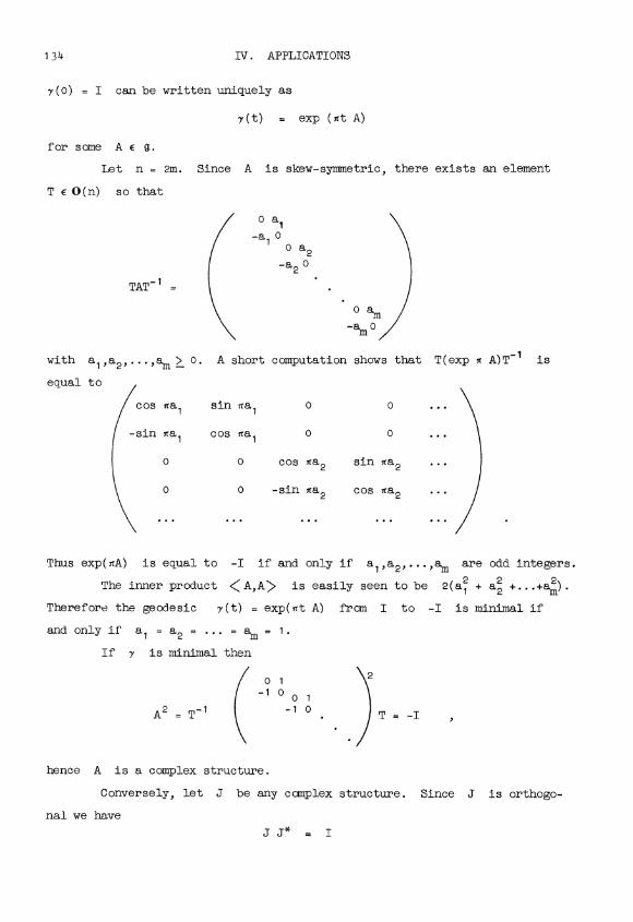
134 IV. APPLICATIONS
y(o) = I can be written uniquely as
y(t) = exp (et A)
for some A E g.
Let n = 2m. Since A is skew-symmetric, there exists an element
T E 0(n) so that
1
TAT-1 =
o a2
-a2 0
o am-am o
with a1,a2,...,am > 0. A short computation shows that T(exp itA)T-1
is
equal to
cos na1 sin aa1 0 0
-sin oat cos rta1 0 0
0 0 cos na2 sin aa2
-a1 0
0 -sin na2 cos na2
Thus exp(aA) is equal to -I if and only if a1,a2,...,a, are odd integers.
The inner product < A,A> is easily seen to be 2(a? + a2 +...+am).
Therefore the geodesic y(t) = exp(nt A) from I to -I is minimal if
and only if a1 = a2 = ... = am = 1.
If y is minimal then
A2 =T-1
0 1 2-1 0
0 1
-1 0 T = -I
hence A is a complex structure.
Conversely, let J be any complex structure. Since J is orthogo-
nal we have
J J* = I

§24. THE ORTHOGONAL GROUP 1 35
where J* denotes the transpose of J. Together with the identity
J J = -I this implies that J = -J. Thus J is skew-symmetric. Hence
T J T-1=
/ o a1
1-a 01
for some a1,a2,...,am > 0 and some T. Now the identity J2 = -I implies
that a1 = ... = ah1 = 1; and hence that exp itJ = -I. This completes the
proof.
LEMMA 24.2. Any non-minimal geodesic from I to -I
in O(2m) has index > 2m-2.
The proof is similar to that of 23.2. Suppose that the geodesic has
the form t -+ exp(at A) with
A =
where a1 > a2 > ... > am > 0 are odd integers. Computation shows that the
non-zero eigenvalues of the linear transformation KA = - -147 (Ad A) 2 are
1) for each i < j the number (ai + aj)2/ 4, and
2) for each i < j with ai # aj the number (ai - aj)2/ 4.
Each of these eigenvalues is to be counted twice. This leads to the formula
I (a + aj - 2) + I (ai - aj - 2)i<j ai>aj
For a minimal geodesic we have a1 = a2 = ... = am = 1 so that
>v = 0, as expected. For a non-minimal geodesic we have a1 > 3; so that
(3+1-2) + 0 = 2m - 2.
This completes the proof.
Now let us apply Theorem 22.1. The two lemmas above, together with

136 TV. APPLICATIONS
the statement that SL1(n) is a manifold imply the following.
THEOREM 24.3 (Bott). The inclusion map 111(n) -+ o 0(n)
induces isomorphisms of homotopy groups in dimensions
< n-4. Hence
Ai a, (n) = ni+1 0(n)for i < n-4.
Now we will iterate this procedure, studying the space of geodesics
from J to -J in f1(n); and so on. Assume that n is divisible by a
high power of 2.
Let J1,...,Jk-1 be fixed complex structures on Rn which anti-
commute *, in the sense that
iris+ Jsir = 0
for r s. Suppose that there exists at least one other complex structure
J which anti-commutes with J1,...,Jk-1'
DEFINITION. Let SLk(n) denote the set of all complex structures J
on Rn which anti-commute with the fixed structures J1,...,Jk-1'
Thus we have
SLk(n) C SLk-1 (n) C ... C SL1 (n) C 0(n)
Clearly each SLk(n) is a compact set. To complete the definition it is
natural to define n0(n) to be 0(n)
LEMMA 24.4. Each SLk(n) is a smooth, totally geodesic**
submanifold of 0(n). The space of minimal geodesics from
JR to -JR in SLR(n) is homeomorphic to SLR+1(n), for
0<R <k.
It follows that each component of SLk(n) is a symmetric space.
For the isometric reflection of 0(n) in a point of SLk(n) will automati-
cally carry ilk(n) to itself.
These structures make Rn into a module over a suitable Clifford algebra.
However, the Clifford algebras will be suppressed in the following presen-
tation.
** A submanifold of a Riemannian manifold is called totally geodesic if
each geodesic in the submanifold is also a geodesic in larger manifold.

§24. THE ORTHOGONAL GROUP 137
PROOF of 24.4. Any point in 0(n) close to the identity can be
expressed uniquely in the form exp A, where A is a "small," skew-
symmetric matrix. Hence any point in 0(n) close to the complex structure
J can be expressed uniquely as J exp A; where again A is small and
skew.
ASSERTION 1. J exp A is a complex structure if and only if A
anti-commutes with J.
PROOF: If A anti-commutes with J, then J-1A J = -A hence
I = exp(J-1A J) exp A =J-1 (exp A)J exp A
Therefore (J exp A)2 = -I. Conversely if (J exp A)2 = -I then the
above computation shows that
exp(J-1A J) exp A = I
Since A is small, this implies that
J-1A J = -A
so that A anti-commutes with J.
ASSERTION 2. J exp A anti-commutes with the complex structures
J1,...,Jk-1 if and only if A commutes with J1,...,Jk-1'
The proof is similar and straightforward.
Note that Assertions I and 2 both put linear conditions on A.
Thus a neighborhood of J in Qk(n) consists of all points J exp A where
A ranges over all small matrices in a linear subspace of the Lie algebra g.
This clearly implies that SLk(n) is a totally geodesic submanifold of
0(n).Now choose a specific point Jk E SLl(n), and assume that there
exists a complex structure J which anti-commutes with J1,...,Jk. Setting
J = JkA we see easily that A is also a complex structure which anti-
commutes with Jk. However, A comutes with J1,...,Jk-1. Hence the
formula
t -Jk exp(st A)
defines a geodesic from Jk to -Jk in Sbk(n). Since this geodesic is
minimal in 0(n), it is certainly minimal in SLk(n).

138 IV. APPLICATIONS
Conversely, let y be any minimal geodesic from Jk to -Jk in
ak(n). Setting y(t) = Jk exp(st A), it follows from 24.1 that A is
a complex structure, and from Assertions 1,2 that A commutes with
J1,...,Jk-1 and anti-commutes with Jk. It follows easily that JA
belongs to fk+1(n). This completes the proof of 24.4.
REMARK. The point JkA enk+1(n) which corresponds to a given
geodesic y has a very simple interpretation: it is the midpoint y(z)
of the geodesic.
In order to pass to a stable situation, note that Ilk(n) can be
imbedded in nk(n+n') as follows. Choose fixed anti-commuting complex
structures J e Slk(n) determines a complex
structure J ® Jk on Rn ®Rn' which anti-commutes with Ja E) J.1, for
a = 1,...,k-1.
DEFINITION. Let 12k denote the direct limit as n--' w of the
spaces ak(n), with the direct limit topology. (I.e., the fine topology.)
The space 0 =110 is called the infinite orthogonal group.
It is not difficult to see that the inclusions 11k+1(n) - n ak(n)
give rise, in the limit, to inclusions 11k+1 -+ nilk '
THEOREM 24.5. For each k > 0 this limit map 1k+1
nllk is a homotopy equivalence. Thus we have isomorphisms
nh 0 = nh-1 111 ah-2112 = ... - "1 ah_lThe proof will be given presently.
Next we will give individual descriptions of the manifolds llk(n)
for k = 0,1,2,...,8.
n0(n) is the orthogonal group.
a1(n) is the set of all complex structures on Rn
Given a fixed complex structure J1 we may think of Rn as being a vector
space CnJ2 over the complex numbers.
n2(n) can be described as the set of "quaternionic structures" on
the complex vector space C2. Given a fixed J. e 112(n) we may think ofn/
§24. THE ORTHOGONAL GROUP 139
Cn/2 as being a vector space He/4 over the quaternions H. Let Sp(n/4)
be the group of isometries of this vector space onto itself. Then SL 2(n)
can be identified with the quotient space U(n/2)/ Sp(n/4).
Before going further it will be convenient to set n = 16r.
LEMMA 24.6 - (3). The space l3(16r) can be identified
with the quaternionic Grassmann manifold consisting of
all quaternionic subspaces of H4r
PROOF: Any complex structure J3 E a3(16r) determines a splitting
of H4r = R16r into two mutually orthogonal subspaces V1 and V2 as fol-
lows. Note that J1J2J3 is an orthogonal transformation with square
J1J2J3J1J2J3 equal to + I. Hence the eigenvalues of J1J2J3 are + 1.
Let V1 C R16r be the subspace on which J1J2J3 equals + I; and let V.
be the orthogonal subspace on which it equals -I. Then clearly
R16r = V1 ® V2. Since J1J2J3 commutes with J1 and J2 it is clear
that both V1 and V2 are closed under the action of J1 and J2.
Conversely, given the splitting H4r = V1 (D V2 into mutually
orthogonal quaternionic subspaces, we can define J3 E a3(16r) by the
identities
J3IV1=
-J1J2lV1
J3IV2 = J1J21V2
This proves Lemma 24.6 -(3).
The space a3(16r) is awkward in that it contains components of
varying dimension. It is convenient to restrict attention to the component
of largest dimension: namely the space of 2r-dimensional quaternionic sub-
spaces of H4r. Henceforth, we will assume that J3 has been chosen in
this way, so that dimes V1 = dimes V2 = 2r.
LEMMA 24.6 - (4). The space n4(16r) can be identified
with the set of all quaternionic isometries from V1 to
V2. Thus Sl4(16r) is diffeomorphic to the symplectic
group Sp(2r).
PROOF: Given J4 E n4(16r) note that the product J3J4 anti-
commutes with J1J2J3 . Hence J3J4 maps V1 to V2 (and V2 to V1).

140 IV. APPLICATIONS
Since J3J4 commutes with J1 and J2 we see that
J3J4fV1 : V1 - V2
is a quaternionic isomorphism. Conversely, given any such isomorphism
T : V1 -. V2 it is easily seen that J4 is uniquely determined by the
identities:
J4IV1 = J31 T
J4IV2 = -T-1 J3
This proves 24.6 - (4).
LEMMA 24.6 - (5). The space Sl5(16r) can be identified
with the set of all vector spaces W C V1 such that
(1) W is closed under J1 (i.e., W is a complex
vector space) and
(2) V1 splits as the orthogonal sum W ® J2 W.
PROOF: Given J5 ea5(16r) note that the transformation J1J4J5
commutes with J1J2J3 and has square + I. Thus J1J4J5 maps V1 into
itself; and determines a splitting of V1 into two mutually orthogonal sub-
spaces. Let W C V1 be the subspace on which J1J4J5 coincides with + I.
Since J2 anti-commutes with J1J4J5, it follows that J2W C V1 is
precisely the orthogonal subspace, on which J1J4J5 equals -I. Clearly
J1W = W.
Conversely, given the subspace W, it is not difficult to show that
J5 is uniquely determined.
REMARK. If U(2r) C Sp(2r) denotes the group of quaternionic auto-
morphisms of V1 keeping W fixed, then the quotient space Sp(2r)/ U(2r)
can be identified with a5(16r).
LEMMA 24.6 - (6). The space Sl6(16r) can be identified
with the set of all real subspaces X C W such that W
splits as the orthogonal sum X ® J1X.
PROOF. Given J6 e a6(16r) note that the transformation J2J4J6
commutes both with J1J2J3 and with J1J4J5. Hence J2J4J6 maps W into
itself. Since (J2J4J6)2 = I, it follows that J2J4J6 determines a
§24. THE ORTHOGONAL GROUP 141
splitting of W into two mutually orthogonal subspaces. Let X C W be the
subspace on which J2J4J6 equals +I. Then J1X will be the orthogonal
subspace on which it equals -I.
Conversely, given X C W, it is not hard to see that J6 is unique-
ly determined.
REMARK. If O(2r) C U(2r) denotes the group of complex automor-
phisms of W keeping X fixed, then the quotient space U(2r)/ O(2r) can
be identified with a 6(16r).
LEMMA 24.6 - (7). The space Sl7(16r) can be identified
with the real Grassmann manifold consisting of all real
subspaces of X = R2r.
PROOF: Given J7, anti-commuting with J1, ... ,J6 note that
J1J6J7 commutes with J1J2J3, with J1J4J5, and with J2J4J6; and has
square +I. Thus J1J6J7 determines a splitting of X into two mutually
orthogonal subspaces: X1 (where J1J6J7 equals +I) and X2 (where
J1J6J7 equals -I). Conversely, given X1 C X it can be shown that J7
is uniquely determined.
This space 117(16r), like J1 3(16r), has components of varying dimen-
sion. Again we will restrict attention to the component of largest dimen-
sion, by assuming that
Thus we obtain:
dim X1 = dim X2 = r.
ASSERTION. The largest component of a7(16r) is diffeomorphic to
the Grassmann manifold consisting of r-dimensional subspaces of R2r.
LEMMA 24.6 - (8). The space fl8(16r) can be identified
with the set of all real isometries from X1 to X2.
PROOF. If J8 e j8(16r) then the orthogonal transformationJ7`T8
commutes with J1J2J3, J1J4J5, and J2J4J6; but anti-commutes with J,J6J7.
Hence J7J8 maps X1 isomorphically onto X2. Clearly this isomorphism
determines J8 uniquely.
Thus we see that d18(16r) is diffeomorphic to the orthogonal
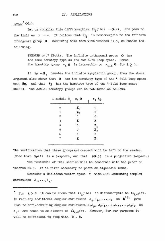
142 IV. APPLICATIONS
group* 0(r).
Let us consider this diffeomorphism Sl8(16r) - 0(r), and pass to
the limit as r -+ -. It follows that Sl8 is homeomorphic to the infinite
orthogonal group O. Combining this fact with Theorem 24.5, we obtain the
following.
THEOREM 24.7 (Bott). The infinite orthogonal group 0 has
the same homotopy type as its own 8-th loop space. Hence
the homotopy group ai 0 is isomorphic to "i+8 0 for i > 0.
If Sp =114 denotes the infinite symplectic group, then the above
argument also shows that 0 has the homotopy type of the 4-fold loop space
0000 Sp, and that Sp has the homotopy type of the 4-fold loop space0000 O. The actual homotopy groups can be tabulated as follows.
i modulo 8 ni O ni Sp
0 Z2 0
1 Z2 0
2 0 0
3 Z Z
4 0 Z2
5 0 Z26 0 0
7 Z Z
The verification that these groups are correct will be left to the reader.
(Note that Sp(1) is a 3-sphere, and that S0(3) is a projective 3-space.)
The remainder of this section will be concerned with the proof of
Theorem 24.5. It is first necessary to prove an algebraic lemma.
Consider a Euclidean vector space V with anti-commuting complex
structures J1,...,Jk.
*For k > 8 it can be shown that dlk(16r) is diffeomorphic to Slk_8(r).
In fact any additional complex structures J9,J10,...,Jk on R16r give
rise to anti-commuting complex structures J8J9, J8J10, J8J111...,J81k on
X1; and hence to an element of fl k_8(r). However, for our purposes it
will be sufficient to stop with k = B.

§24. THE ORTHOGONAL GROUP 143
DEFINITION. V is a minimal (J1,...,Jk)-space if no proper, non-
trivial subspace is closed under the action of J1,..., and Jk. Two such
minimal vector spaces are isomorphic if there is an isometry between them
which commutes with the action of J1,...,Jk.
LEMMA 24.8 (Bott and Shapiro). For k 3 (mod 4), any
two minimal (J1,...,Jk) vector spaces are isomorphic.
The proof of 24.8 follows that of 24.6. For k = 0,1, or 2 a
minimal space is just a 1-dimensional vector space over the re als, the
complex numbers or the quaternions. Clearly any two such are isomorphic.
For k = 3 a minimal space is still a 1-dimensional vector space
over the quaternions. However, there are two possibilities, according as
J3 is equal to +J1J2 or -J1J2. This gives two non-isomorphic minimal
spaces, both with dimension equal to 4. Call these H and H'.
For k = 4 a minimal space must be isomorphic to H ® H', with
J3J4 mapping H to H'. The dimension is equal to 8.
For k = 5,6 we obtain the same minimal vector space H ® H'. The
complex structures J5,J6 merely determine preferred complex or real sub-
spaces. For k = 7 we again obtain the same space, but there are two
possibilities, according as J7 is equal to +J1J2J3J4J5J6 or to
-J1J2J3J4J5J6. Thus in this case there are two non-isomorphic minimal
vector spaces; call these L and L'.
For k = 8 a minimal vector space must be isomorphic to L ® L',
with J7J8 mapping L onto L'. The dimension is equal to 16.
For k > 8 it can be shown that the situation repeats more or less
periodically. However, the cases k < 8 will suffice for our purposes.
Let mk denote the dimension of a minimal (J1,...,Jk)-vector space.
From the above discussion we see that:
m0 = 1, m1 = 2, m2 = m3 = 4,
m4 = m5 = m6 = m7 = 8, m8 = 16.
For k > 8 it can be shown that mk = 16mk-8.
REMARK. These numbers mk are closely connected with the problem
of constructing linearly independent vector fields on spheres. Suppose for
example that J1,...,Jk are anti-commuting complex structures on a vector

144 IV. APPLICATIONS
space V of dimension rmk. Here r can be any positive integer. Then
for each unit vector u E V the k vectors J1u, J2u,..., Jku are perpen-
dicular to each other and to u. Thus we obtain k linearly independent
vector fields on an (rmk 1)-sphere. For example we obtain 3 vector
fields on a (4r-1)-sphere; 7 vector fields on an (8r-1)-sphere; 8 vector
fields on a (16r-1)-sphere; and so on. These results are due to Hurwitz
and Radon. (Compare B. Eckmann, Gruppentheoretischer Beweis des Satzes von
Hurwitz-Radon..., Commentarii Math. Hely. Vol. 15 (1943), pp. 358-366.) J.
F. Adams has recently proved that these estimates are best possible.
PROOF of Theorem 24.5 for k V 2 (mod 4). We must study non-
minimal geodesics from J to -J in 11k(n). Recall that the tangent space
of 11k(n) at J consists of all matrices J A where
1) A is skew
2) A anti-commutes with J
3) A commutes with J1,".,Jk-1'
Let T denote the vector space of all such matrices A. A given A E T
corresponds to a geodesic t - J exp (at.4) from J to -J if and only if
its eigenvalues are all odd multiples of i.
Each such A E T determines a self-adjoint transformation
KA: T - T. Since a k(n) is a totally geodesic submanifold of 0(n), we
can compute KA by the formula
KAB = -1 [A,[A,B1] _ (-A2B + 2ABA - BA2)/4 ,
just as before. We must construct some non-zero eigenvalues of KA so as
to obtain a lower bound for the index of the corresponding geodesic
t - J exp(irt A) .
Split the vector space Rn as a direct sum M1 ® M2 ® ... ® Ms of
mutually orthogonal subspaces which are closed and minimal under the action
of J1,...,Jk-1, J and A. Then the eigenvalues of A on Mh must be
all equal, except for sign.* For otherwise Mh would split as a sum of
*We are dealing with the complex eigenvalues of a real, skew-symmetric
transformation. Hence these eigenvalues are pure imaginary; and occur in
conjugate pairs.
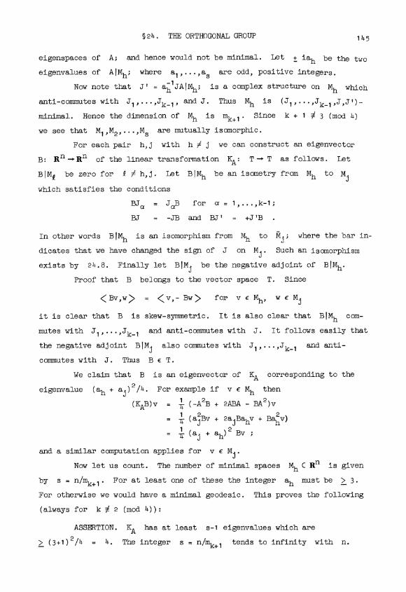
§24. THE ORTHOGONAL GROUP 145
eigenspaces of A; and hence would not be minimal. Let + iah be the two
eigenvalues of AIMh; where a1,...,as are odd, positive integers.
Now note that J' = ah1JAIMh; is a complex structure on Mh which
anti-commutes with J1,...,Jk-1, and J. Thus Mh is (J1,...,Jk-1,J,J')-
minima].. Hence the dimension of Mh is mk+1 Since k + 1 3 (mod 4)
we see that M1,M2,...,Ms are mutually isomorphic.
For each pair h,j with h j we can construct an eigenvector
B: Rn _Rn of the linear transformation KA: T - T as follows. Let
BIM, be zero for f / h,j. Let BIMh be an isometry from Mh to Mj
which satisfies the conditions
BJa = J0B for a = 1,...,k-1;
BJ = -JB and BJ' = +J'B .
In other words BIMh is an isomorphism from Mh to Mj; where the bar in-
dicates that we have changed the sign of J on Mj. Such an isomorphism
exists by 24.8. Finally let BIMj be the negative adjoint of BIMh.
Proof that B belongs to the vector space T. Since
<Bv,w> = Kv,- Bw> for v E Mh, w E Mj
it is clear that B is skew-symmetric. It is also clear that BIMh com-
mutes with J1,...,Jk-1 and anti-commutes with J. It follows easily that
the negative adjoint BIMj also commutes with J1,...,Jk-1 and anti-
commutes with J. Thus B E T.
We claim that B is an eigenvector of KA corresponding to the
eigenvalue (ah + aj)2/4. For example if v e Mh then
(KAB)v = (-A2B + 2ABA - BA2)v
72ajBahv + Bahv)
_ (aj + ah) 2 By-IT
and a similar computation applies for v E Mj.
Now let us count. The number of minimal spaces Mh C Rn is given
by s = n/mk+1' For at least one of these the integer ah must be > 3.
For otherwise we would have a minimal geodesic. This proves the following
(always for k 2 (mod 4)):
ASSERTION. KA has at least s-1 eigenvalues which are
> (3+1)2/4 = 4. The integer s = n/mk+1 tends to infinity with n.

146 IV. APPLICATIONS
Now consider the geodesic t -+ J exp(at A). Each eigenvalue e2
of KA gives rise to conjugate points along this geodesic for
t = e-1, 2e-1, 3e-1,... by 20.5. Thus if e2 > 4 then one obtains at
least one interior conjugate point. Applying the index theorem, this proves
the following.
ASSERTION. The index of a non-minimal geodesic from J to -J in
Slk(n) is > n/mk+1- 1.
It follows that the inclusion map
ak+1(n) -+ o nk(n)
induces isomorphisms of homotopy groups in dimensions < n/mk+1 - 3. This
number tends to infinity with n. Therefore, passing to the direct limit
as n -+ co, it follows that the inclusion map i : S?,k+1 -i a S).k induces
isomorphisms of homotopy groups in all dimensions. But it can be shown
that both SZk+1 and a Dk have the homotopy type of a CW-complex. There-
fore, by Whitehead's theorem, it follows that i is a homotopy equivalence.
This completes the proof of 24.5 providing that k 0 2 (mod 4).
PROOF of 24.5 for k e 2 (mod 4). The difficulty in this case may
be ascribed to the fact. that dlk(n) has an infinite cyclic fundamental
group. Thus nilk(n) has infinitely many components, while the approximat-
ing subspace fk+1(n) has only finitely many.
To describe the fundamental group allk(n) we construct a map
f : dlk(n) -o S1 C C
as follows. Let J1,...,Jk-1 be the fixed anti-commuting complex struc-
ture on R. Make Rn into an (n/2)-dimensional complex vector space by
defining
iv = J1 J2 ... Jk-1v
for v e Rn; where i = 47-1 E C. The condition k 2 (mod 4) guarantees
that i2 = -1, and that J1,J21...IJk-1 commute with i.
Choose a base point J e llk(n) . For any J' e Slk(n) note that thecomposition J-1J' commutes with i. Thus J-1J' is a unitary complex
linear transformation, and has a well defined complex determinant which will
be denoted by f(J').

§24. THE ORTHOGONAL GROUP 147
Now consider a geodesic
t J exp(sctA)
from J to -J in 1Zk(n). Since A commutes with i = J1J2 ... Jk-1
(compare Assertion 2 in the proof of 24.4) we may think of A also as a
complex linear transformation. In fact A is skew-Hermitian; hence the
trace of A is a pure imaginary number. Now
f(J exp(stA)) = determinant (exp(stA)) = ent trace A
Thus f maps the given geodesic into a closed loop on S1 which is com-
pletely determined by the trace of A. It follows that this trace is in-
variant under homotopy of the geodesic within the path space n(11k(n);J,-J).
The index % of this geodesic can be estimated as follows. As
before split Rn into an orthogonal sum M1 ® ... ® Mr where each Mh
is closed under the action of J1,...,Jk-1,J, and A; and is minimal.
Thus for each h, the complex linear transformation AIMh can have only
one eigenvalue, say iah. For otherwise Mh would split into eigenspaces.
Thus AIMh coincides with ahJlJ2 ... Jk-1IMh. Since Mh is minimal under
the action of J1,...,Jk-1, and J; its complex dimension is mk/2.
Therefore the trace of A is equal to i(a1+...+ar)mk/2.
Now for each h X j an eigenvector B of the linear transforma-
tion
B -+ KAB = (-A2B + 2ABA - BA2) /4
can be constructed much as before. Since Mh and Mj are (J1,...,Jk-1,J)-
minimal it follows from 24.8 that there exists an isometry
BIMh : Mh-> Mj
which commutes with J1,...,Jk-1 and anti-commutes with J. Let BIMj be
the negative adjoint of BIMh; and let BIM1 be zero for e / h,j. Then
an easy computation shows that
KAB = (ah - aj) 2B/4
Thus for each ah > aj we obtain an eigenvalue (ah - aj)2/4 for KA.
Since each such eigenvalue makes a contribution of (ah - aj)/2 - 1
towards the index x, we obtain the inequality
2 ) , > (ah- aj - 2)ah > aj
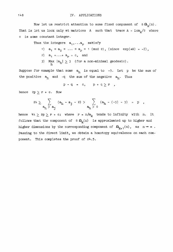
148 TV. APPLICATIONS
Now let us restrict attention to some fixed component of Q ak(n).
That is let us look only at matrices A such that trace A = icmk/2 where
c is some constant integer.
Thus the integers al,...ar satisfy
1) a, a a2 = ... = ar (mod 2), (since exp(aA) = -I),
2) al +...+ ar = c, and
3) Max lahi > 3 (for a non-minimal geodesic).h
Suppose for example that some ah is equal to -3. Let p be the sum of
the positive ah and -q the sum of the negative ah. Thus
p-q = c, p+q>r ,
hence 2p > r + c. Now
2X > (ah - a - 2) > (ah - (-3) - 3) = pah>a3 ah>o
hence 4X > 2p > r + c; where r = n/mk tends to infinity with n. It
follows that the component of C 11k(n) is approximated up to higher and
higher dimensions by the corresponding component of Sk+l(n), as n - C .
Passing to the direct limit, we obtain a homotopy equivalence on each com-
ponent. This completes the proof of 24.5.
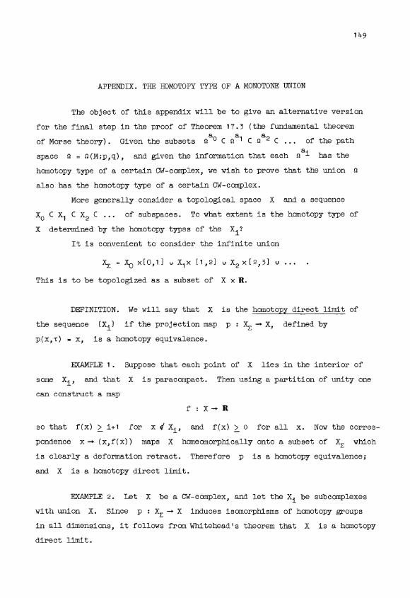
149
APPENDIX. THE HOMOTOPY TYPE OF A MONOTONE UNION
The object of this appendix will be to give an alternative version
for the final step in the proof of Theorem 17.3 (the fundamental theorem
of Morse theory). Given the subsets oao C a1 C saa2 C ... of the patha
space o = o(M;p,q), and given the information that each o i has the
homotopy type of a certain CW-complex, we wish to prove that the union 0
also has the homotopy type of a certain CW-complex.
More generally consider a topological space X and a sequence
X0 C X1 C X2 C ... of subspaces. To what extent is the homotopy type of
X determined by the homotopy types of the Xi?
It is convenient to consider the infinite union
X£ = X0 x[0,1] v X1X (1,2] u X2 X(2,31 u ...
This is to be topologized as a subset of X x R.
DEFINITION. We will say that X is the homotopy direct limit of
the sequence (Xi) if the projection map p : X£ - X, defined by
p(x,T) = x, is a homotopy equivalence.
EXAMPLE 1. Suppose that each point of X lies in the interior of
some Xi, and that X is paracompact. Then using a partition of unity one
can construct a map
f : X- R
so that f(x) > i+1 for x Xi, and f(x) > 0 for all x. Now the corres-
pondence x - (x,f(x)) maps X homeomorphically onto a subset of X. which
is clearly a deformation retract. Therefore p is a homotopy equivalence;
and X is a homotopy direct limit.
EXAMPLE 2. Let X be a CW-complex, and let the Xi be subcomplexes
with union X. Since p : X£ - X induces isomorphisms of homotopy groups
in all dimensions, it follows from Whitehead's theorem that X is a homotopy
direct limit.

150 APPENDIX
EXAMPLE 3. The unit interval [0,1] is not the homotopy direct
limit of the sequence of closed subsets [o] v [1/i,1].
The main result of this appendix is the following.
THEOREM A. Suppose that X is the homotopy direct
limit of [X.1 and Y is the homotopy direct limit
of {Yi). Let f: X Y be a map which carries each
Xi into Yi by a homotopy equivalence. Then f
itself is a homotopy equivalence.
Assuming Theorem A, the alternative proof of Theorem 17.3 can be
given as follows. Recall that we bad constructed a commutative diagram
S2ao C saa, C saa2 C ...
Ko C K1 C K2 C ...
aof homotopy equivalences. Since 1a = U o i and K = U Ki are homotopy
direct limits (compare Examples I and 2 above), it follows that the limit
mapping 0- K is also a homotopy equivalence.
PROOF of Theorem A. Define f£ : XX -* YY by f£(x,t) = (f(x),t).
It is clearly sufficient to prove that f£ is a homotopy equivalence.
CASE 1. Suppose that Xi = Yi and that each map fi : Xi-.. Yi
(obtained by restricting f) is homotopic to the identity. We must prove
that f£ is a homotopy equivalence.
REMARK. Under these conditions it would be natural to conjecture
that f. must actually be homotopic to the identity. However counter-
examples can be given.
For each n let
Xn Xn
be a one-parameter family of mappings, with hn fn, hn = identity.
Define the homotopy
h : Xz - X&

HOMOTOPY OF A MONOTONE UNION 151
as follows (where it is always to be understood that 0 < t < 1, and
n = 0,1,2,...).
(hu(x),n+2t) for 0 < t < z
hu(x,n+t) (h(3-4t)u (x),n+1) for z < t < -T
0,,n+3
(x),n+1)for < t < 1
Taking u = 0 this defines a map h0 : XE X£ which is clearly homotopic
to fE. The mapping h1 : XE XE on the other hand has the following
properties:
h1(x,n+t) = (x,n+2t) for 0 < t < z
+1 x[n+11 for 2 < t < 1h1(x,n+t) e 71,
We will show that any such map h1 is a homotopy equivalence. In fact a
homotopy inverse g : XE - XE can be defined by the formula
((x,n+2t) 0 < t <
g(x,n+t) = j - -1 < t < 1l h (x,n 2- t) 2
This is well defined since
h1(x,n+2) = h1(x,n+1) = (x,n+1) .
Proof that the composition h1g is homotopic to the identity map
of XE. Note that
(x,n+4t) 0 < t < 4
h1g(x,n+t) = h1(x,n+2t) 4 < t < 2
h1 (X,ri 2 - t) 2 < t < 1
Define a homotopy Hu : XE XE as follows. For 0 < u < z let
h1g(x,n+t) for 0 < t < (1-u)/2
Hu(x,n+t) = and for z+u < t < 1
h1(x,n+1-u) for (1-u)/2 < t < z + U.

152 APPENDIX
This is well defined since
h1g(x,n+(1-u)/2) = h1g(x,n+2+u) = h1(x,n+1-u).
Now Ho is equal to h1g and Hiz is given by
1(x,n+4t) 0 < t < 4
Hi(x,n+t)z =
(x,n+1) < t < 1
Clearly this is homotopic to the identity.
Thus h1g is homotopic to the identity; and a completely analogous
argument shows that gh1 is homotopic to the identity. This completes the
proof in Case 1.
CASE 2. Now let X and Y be arbitrary. For each n let
gn : Yn -+ Xn be a homotopy inverse to fn. Note that the diagram
griYn Xn
Iin tingYl+ 1
Yn+1 Xn+1
(where in and in denote inclusion maps) is homotopy commutative. In
fact
1ngn ti gnifn+tingn = gn+tjnfngn - gn+1jn
Choose a specific homotopy hu : Yn--' Xn+1 with ho = ingn, h, gn+1Jn;
and define G : Y£ X£ by the formula
(gn(y),n+2t) 0 < t <
G(y,n+t)
(h2t-1(y),n+1) < t < 1
We will show that the composition Gf£ : X£ -+ X. is a homotopy equivalence.
Let X£ denote the subset of XE consisting of all pairs (x,T) with
T < n. (Thus X£ = X0 x[o,11 ... Xn_1 x [n-1 n] u Xn x[n].) The compo-
sition Gf£ carries X2 into itself by a mapping which is homotopic to the
identity. In fact X£ contains Xn x[n] as deformation retract; and the
mapping GfE restricted to Xn x[n] can be identified with gnfn, and
hence is homotopic to the identity. Thus we can apply Case 1 to the sequence
HOMOTOPY OF A MONOTONE UNION 153
(X£n} and conclude that Gf£ is a homotopy equivalence.
This proves that f. has a left homotopy inverse. A similar
argument shows that f£G : Y£ - Y. is a homotopy equivalence, so that
f£ has a right homotopy inverse. This proves that f£ is a homotopy
equivalence (compare page 22) and completes the proof of Theorem A.
COROLLARY. Suppose that X is the homotopy direct
limit of (Xi). If each Xi has the homotopy type
of a OW-complex, then X itself has the homotopy
type of a OW-complex.
The proof is not difficult.

ANNALS OF MATHEMATICS STUDIES
EDITED BY Luis A. CAFFARELLI, JOHN N. MATHER, and ELIAS M. STEIN
142. Renormalization and 3-Manifolds which Fiber over the Circle, by CURTIS T.MCMULLEN
141. Period Spaces for p-divisible Groups, by M. RAPOPORT and TH. ZINK
140. Global Surgery Formula for the Casson-Walker Invariant, by CHRISTINE. Lesco
139. Rigid Local Systems, by NICHOLAS M. KATz
138. Prospects in Topology: Proceedings of a Conference in Honor of William Browder,edited by FRANK QUINN
137. Modern Methods in Complex Analysis: The Princeton Conference in Honor ofGunning and Kohn, edited by THOMAS BLOOM, DAVID CATLIN, JOHN P. D'ANGELO,and YUM-TONG SIU
136. Hyperfunctions on Hypo-Analytic Manifolds, by PAULO D. CORDARO and FRANCOISTREVES
135. Complex Dynamics and Renormalization. by CURTIS T. MCMULLEN
134. Temperley-Lieb Recoupling Theory and Invariants of 3-Manifolds, by Louis H.KAUEEMAN and SOSTENES L. LINS
133. An Introduction to G-Functions. by BERNARD DwoRK. GIOVANNI GERorro. andFRANCIS J. SULLIVAN
132. Commensurabilities among Lattices in PU(l.n), by PIERRE DELIGNE and G. DANIELMOSTOW
131. Introduction to Toric Varieties. by WILLIAM FULTON
130. Harmonic Maps and Minimal Immersions with Symmetries, by JAMES EELLSand ANDREA RATIO
129. The Admissible Dual of GL(N) via Compact Open Subgroups, by COLIN J.BUSHNELL and PHILIP C. KUTZKO
128. Nilpotence and Periodicity in Stable Homotopy Theory. by DOUGLAS C.RAVENEL
127. Lectures on the Arithmetic Riemann-Roch Theorem, by GERD FALTINGS
126. An Extension of Casson's Invariant, by KEVIN WALKER
125. Combinatorics of Train Tracks, by R. C. PENNER with J. L. HARER
124. Exponential Sums and Differential Equations. by NICHOLAS M. KATz
123. Automorphic Representations of Unitary Groups in Three Variables, byJONATHAN D. ROGAWSKI
122. Harmonic Analysis in Phase Space. by GERALD B. FOLLAND
121. Cosmology in (2 + 1)-Dimensions, Cyclic Models, and Deformations of M,.,, byVICTOR GUILLEMIN
120. Simple Algebras, Base Change, and the Advanced Theory of the Trace Formula, byJAMES ARTHUR and LAURENT CLOZEL
A complete catalogue of Princetonmathematics and science books, with ISBN 0-691-08008-9prices, is available upon request. 90000PRINCETON UNIVERSITY PRESS
91111111111111111111111111111111111111111111111
41 WILLIAM STREET 780691 080086PRINCETON, NEW JERSEY 08540
Recommended