Natural Computing Series

Multiobjective Problem Solving from Nature

From Concepts to Applications

Bearbeitet vonJoshua Knowles, David Corne, Kalyanmoy Deb

1. Auflage 2007. Buch. xvi, 411 S. HardcoverISBN 978 3 540 72963 1

Format (B x L): 15,5 x 23,5 cm

Weitere Fachgebiete > Mathematik > Operational Research > Spieltheorie

Zu Inhaltsverzeichnis

schnell und portofrei erhältlich bei

Die Online-Fachbuchhandlung beck-shop.de ist spezialisiert auf Fachbücher, insbesondere Recht, Steuern und Wirtschaft.Im Sortiment finden Sie alle Medien (Bücher, Zeitschriften, CDs, eBooks, etc.) aller Verlage. Ergänzt wird das Programmdurch Services wie Neuerscheinungsdienst oder Zusammenstellungen von Büchern zu Sonderpreisen. Der Shop führt mehr

als 8 Millionen Produkte.

Introduction: Problem Solving, EC and EMO

Joshua Knowles1, David Corne2, and Kalyanmoy Deb3

1 School of Computer Science, University of Manchester, UKj.knowles@manchester.ac.uk

2 School of Mathematical and Computer Sciences (MACS), Heriot-WattUniversity, Edinburgh, UK dwcorne@macs.hw.ac.uk

3 Kanpur Genetic Algorithms Laboratory (KanGAL), Indian Institute ofTechnology, Kanpur, India deb@iitk.ac.in

Summary. This book explores some emerging techniques for problem solving of ageneral nature, based on the tools of EMO. In this introduction, we provide back-ground material to support the reader’s journey through the succeeding chapters.Given here are a basic introduction to optimization problems, and an introductorytreatment of evolutionary computation, with thoughts on why this method is sosuccessful; we then discuss multiobjective problems, providing definitions that somefuture chapters rely on, covering some of the key concepts behind multiobjectiveoptimization. These show how optimization can be carried out separately from sub-jective factors, even when there are multiple and conflicting ends to the optimizationprocess. This leads to a set of trade-off solutions none of which is inherently bet-ter than any other. Both the process of multiobjective optimization, and the setof trade-offs resulting from it, are ripe areas for innovation — for new techniquesfor problem solving. We briefly preview how the chapters of this book exploit theseconcepts, and indicate the connections between them.

1 Overview

Intellectual activity consists mainly of various kinds of search.Alan M. Turing, 1948

When we say that computers can solve problems, it is a sort of half-truth, tobe taken with a medium-sized pinch of salt. It is manifestly true that computerssolve problems when they almost autonomously carry out everyday tasks involvingcommunication, auditing, logistics and so forth, and computers even act somewhatmore ‘intelligently’ when they do such tasks as controlling an automatic transmis-sion, or making a medical diagnosis, in which they may even exhibit a computerizedform of learning. But it is also true that computers are not very autonomous insolving new problems. Much human input and human innovation still goes into theprocess of solving difficult problems (designing a cable-stayed bridge, finding noveldrug interventions, brokering international peace initiatives), a state of affairs thatis likely — and desirably so — to continue for some time to come.

2 Knowles et al.

In this book, we consider an area in computer science which is at the forefrontof techniques for solving difficult problems. Evolutionary computation — that is,methods that resemble a process of Darwinian evolution — can be used as a wayto make computers ‘evolve’ solutions to problems, which we, as humans, do notourselves know how to solve. By giving computers the capability of searching fortheir own answers to problems — through huge spaces of possibilities, in a very flex-ible way that goes beyond numerical methods — innovative and intelligent-seemingsolutions and actions can be produced.

Much of evolutionary computation is concerned with optimization. For a humanto use evolutionary computation to solve a new optimization problem, very little isrequired. This is where the flexibility of EC comes from: one must only provide thecomputer with (i) some way of representing or even ‘growing’ candidate solutions tothe problem, and (ii) some function (or method) for evaluating any candidate solu-tion, estimating its goodness on a numerical scale. Enormous varieties of problemscan be stated succinctly in this way, from electronic circuits to furniture designs,and from strategies for backgammon to spacecraft trajectories. And the boon of evo-lutionary computation (though not one hundred percent realized) is that it turnscomputers into almost universal problem solvers which can be used by anyone witheven minimal computational/mathematical competence. Of course, many problemsare fundamentally intractable, in the sense that we cannot hope to find truly optimalsolutions, but this does not really limit the uses of EC, but makes it more useful,since its strength is in finding the best solution possible given the time allowed.

But, while we just said that optimization is widely applicable, it is but a sub-set of a larger and even more flexible method of problem solving: multiobjectiveoptimization (MOO). The drawback of standard optimization (let’s call it single-objective optimization or SOO) is the requirement for a function that can score eachand every candidate solution in terms of a single objective number. Many problemsexist that are not so easy to state in terms of a single function like this. Humansare generally much more comfortable with, and used to, thinking in terms of aimsand objectives plural, when stating a problem. And, while it is possible, in princi-ple, for people to combine their aims in some over-arching function by weighting orordering them by importance, in practice, different aims and objectives are oftennot measured in the same units, on the same scales, and it is often nigh-impossibleto state the importance of different objectives when one has seen no solutions yet!More fundamentally, many of the methods for combining functions together intoa single one, necessarily miss potentially interesting solutions. And many methodsare very difficult to use because a small change in weights, gives a totally differentsolution. Therefore, it would be great if one could exploit the power of evolutionaryalgorithms, but use them to search for solutions even when the aims and objectivescannot be boiled down to a single function.

We are being purposely obtuse here, of course, because such methods already doexist in the field of evolutionary multiobjective optimization (EMO), and they havebeen growing more and more effective over the past twenty years or so. An EMOalgorithm is, loosely-speaking, one in which objectives are treated independently,and a set of optimal trade-offs (called Pareto optima) is sought, rather than a singleoptimum. But we introduced the field in this roundabout way to emphasise the point,made above, that computers solve problems — difficult problems at least — onlyin concert with humans. Humans are still the ones who generally own the problemsand understand something about what they desire and hope for in a solution. So,

Introduction 3

one of the key hurdles to problem solving with computers is to be able to formulate aproblem in such a way that a computer can actually solve it, and a human is happywith the solution. EMO has this ability in spades, so rather than being a merebranch of EC, it actually represents a major step forward generally in computerproblem solving.

Where this book advances further in terms of problem solving with computers,and problem solving specifically using the tools of evolutionary multiobjective op-timization, is in examining the critical area of how to exploit the greater flexibilityof search afforded by a multiobjective optimization perspective. While other booksand articles on EMO [6, 7, 5] have given a thorough grounding in the developmentof EMO techniques, and have been formidable advocates of its benefits, it is onlyrelatively recently that a groundswell in terms of researchers confidently exploitingEMO tools to new and innovative ends has really been apparent. It is on this weconcentrate.

The new uses of EMO do not represent a step-change, but a gradual realizationthat there are few hard-and-fast rules in solving problems with the technique. Thus,researchers have begun to ask themselves such things as what would happen if Itook away a constraint and treated it as an objective, what would happen if I hada problem where I had one objective but it seemed possible to decompose it intoseveral, what would happen if I had some different functions which were inaccu-rate proxies for a true ideal objective function? In this book, we see how currentresearch is dealing with these questions and further we see valuable products of thisexploration. We see here that, ironically, EMO is very useful in coevolution, an areacharacterized by problems that have no formal objective function at all (evaluationoccurs only by competitions). We see it helps in traditional SOO problems, whereit speeds up search. We see it put to numerous uses in ill-posed problems, especiallythose in machine learning. Along the way, the chapters also consider the importantissue of how to analyse and exploit the sets of solutions that are obtained fromEMO, both in terms of decision making (i.e., usually choosing one final solution) orof learning from the set of trade-offs. And the development of EMO methods withrespect to their scalability to larger problems with more objectives is considered,and supports the ideas proposed throughout the book.

In this chapter, we seek to do two jobs. First, to preview the book, which we havepartly done, but which we continue in Sec. 4. Secondly, to cover some bases for anyreaders who might be unfamiliar with the fundamental concepts whose knowledge isassumed in some of the chapters, we give some appropriate introductory material.To these ends, Sec. 2 recalls the formal definition of a problem, including, in partic-ular, an optimization problem. Hard problems, evolutionary algorithms, and the useof the latter on the former, are then discussed. Sec. 3 deals with multiobjective opti-mization, giving definitions for Pareto optimality and related issues. Then, Sec. 4 isa rundown of the four parts the book is divided into, and provides summaries of eachof the chapters that make it up. Finally, Sec. 5 briefly concludes this introductionchapter.

4 Knowles et al.

2 Problems and Solution Methods

2.1 Optimization Problems

Problems, in computer science, are both abstract and precise. They are abstract inthe sense of describing a whole class of instances; they are nevertheless precise inthe sense that both the inputs and the solution of a problem instance are membersof well-defined (mathematical) sets.

Specifically, a problem consists of: (i) a set of instances, where this set can bedefined by either listing it exhaustively (enumerating it), or, much more usually,by specifying all the givens that define the form of an instance; and (ii) a set ofsolutions, being a definition of the entities that comprise a valid solution and thecriteria for accepting it.

For example, we could define a sorting problem. A valid instance could be definedas any finite set of positive integers; a valid solution as an ordering of the input setthat is strictly increasing.

An optimization problem is just a problem where the solution part of the problemis defined in terms of a function (the objective function), which is to be maximizedor minimized.

Definition 1 An optimization problem is specified by a set of problem instances andis either a minimization problem or a maximization problem.

From here onwards we will consider only minimization problems. In mathemat-ical parlance, this is done ‘without loss of generality’, i.e., everything we say is trueof both minimization and maximization problems, as long as we replace ‘smallest’with ‘largest’ and such like.

Definition 2 An instance of an optimization problem is a pair (X, f), where thesolution set X is the set of feasible solutions and the objective function f is a mappingf : X → �. The problem is to find a globally optimal solution, i.e., an i∗ ∈ X suchthat f(i∗) ≤ f(i) for all i ∈ X. Furthermore, f∗ = f(i∗) denotes the optimal cost,and X∗ = {i ∈ X | f(i) = f∗} denotes the set of optimal solutions.

In this definition, ‘solution’ is being used in a broad sense to mean any well-formedanswer to the problem that maps to a cost through the function f . The objective isnot to find a solution, but to find a minimum cost one. In this case, therefore, it ismeaningful to talk about an approximate solution to the problem, i.e., one that isclose to optimal.

Once the problem is defined, we commonly express the task of optimization –the fact that we wish to minimize our cost function over a particular set of potentialsolutions, as follows:

minimize f(x), subject to x ∈ X. (1)

Here, f is the objective function, and it maps any solution x that is a member ofthe set of feasible solutions X to the set of real numbers, �. We are asked to findan x, such that f is minimized.

Introduction 5

2.2 Hard Optimization Problems

Some optimization problems are easy to solve, and fundamentally so. An easy prob-lem is one where there exists a method that always works — that solves every validinstance — finding an optimal solution in a reasonable amount of time, or number ofsteps. An example of an easy problem is that of finding a shortest path between twonodes in a network, where the nodes are separated by links with certain lengths. Thisproblem can be solved using Dijkstra’s famous algorithm (dynamic programming),an ingenious method that greedily constructs the optimal solution, by consideringpartial paths through the network and keeping track of the competing alternatives.

Unfortunately, a great many problems that we encounter — and almost all ofthose in science and industry — are hard. That is to say, there is no known methodfor solving instances of them exactly and reliably. More than that, these problemsare fundamentally hard in that they can be shown to belong to a set of problems,all of which are essentially equivalent in their difficulty. The equivalence means thatfinding quick and reliable methods for solving one of the problems would result inquick and reliable methods for all of them.

However, no such method has yet been found, and many think that such amethod does not exist. Computer scientists call optimization problems that arefundamentally hard in this way, NP-hard [17].

Consider the following list of problems:

- Find a competent, or good, strategy for playing the game, Othello- Allocate resources for flood protection of the UK- Define a taxonomy of prokaryotic genes, by their functional activities- Design a suspension bridge- Schedule the jobs in a factory, as orders and raw materials arrive periodically.

When defined more precisely, each of these is an example of a fundamentallyhard problem. There is no way to go directly to an optimal solution, or to organizea search in a super-efficient fashion that gives reliable results for all instances.

Instead, for problems like these, we can only hope to find good (or approximatelyoptimal) solutions, by a process of searching through alternatives. Further, beingfundamentally hard, this process is likely to take significant time, even using modernhardware, and even just to find an acceptable, rather than good, solution.

Fortunately, however, we rarely need to resort to a blind, random search throughthe set X. Each of these problems, and realistic problems in general, have someinherent structure that can be exploited as we try to devise a strategy for seekinggood solutions. This structure is usually apparent in the way that similar solutionsare related in terms of the cost function(s). For example, if two suspension bridgedesigns are very similar, but differing slightly in the distance between the points ofsuspension, then the performance characteristics of these two bridges are likely tobe very similar too. Such structure is partly captured by the search landscape; oncewe have settled on the details of X (having decided how we will encode potentialsolutions to the problem), the details of f , and the specifics of how we will generatenew solutions from others previously sampled, this landscape comes to life as a high-dimensional mathematical structure. A fundamental aspect of all modern searchstrategies is to sample points in this landscape (i.e., points in X), and attempt todiscover (or simply assume) certain properties of the landscape in an attempt tonavigate a path through it towards good solutions. One class of such strategies,

6 Knowles et al.

called evolutionary computation, is recognized as being particularly successful (incomparison to other methods, at least) at handling the landscapes found in mostreal-world problems.

2.3 Evolutionary Computation

Algorithms are conceived in analytic purity in the high citadels of aca-demic research, heuristics are midwifed by expediency in the dark cornersof the practitioner’s lair ... and are accorded lower status. Fred Glover

Origins

Problem solving by simulated evolution has been invented independently severaltimes. Its pre-history can be traced back at least to Butler, who pronounced thatthat machines might ‘become as complicated as us’ by evolutionary processes, longbefore general purpose computers had even been conceived (see Dyson [9], chap. 2).Actual computerized simulations began in the 1950s, one of the early notable exam-ples of problem solving being work by Baricelli [1] to ‘evolve’ fragments of code thatcooperated to play a game called Tac-Tix. Fraser [16], Bremmerman [3], Rechen-berg [30], Schwefel [33] and Fogel [14] all experimented with models of evolution inindependent work conducted in the 50s and 60s, and were joined by many others,notably Holland [19] in the 70s. These researchers had very different ends in mind,and emphasised different elements of the neo-Darwinian principles of evolution inthe models that they investigated (for detailed accounts of this early, pioneeringwork see [13] and [9]). For some time, the differences were cemented, and the dis-tinct methods known as evolution strategies, genetic algorithms and evolutionaryprogramming developed in isolation. Today, and since the 1990s, evolutionary com-putation is inclusive of all these areas, and innovations cross the boundaries, usingcommon concepts and abstractions from nature.4

The Basic Evolutionary Algorithm

Despite the high-falutin ideals of evolutionary computation to model and abstractfrom the complexity and richness of nature’s wandering adaptive walks, the basicevolutionary algorithm for optimization has much more in common with a processof selective breeding (as used by Mendel) than it does with adaptation. The opti-mization problem provides a static goal to which the algorithm is directed, and apopulation of solutions are improved towards this by rounds of evaluation, biasedselection, reproduction, variation and replacement. One round or cycle is called ageneration, and the pseudocode in Fig. 1 captures the central process in practicallyevery evolutionary algorithm:

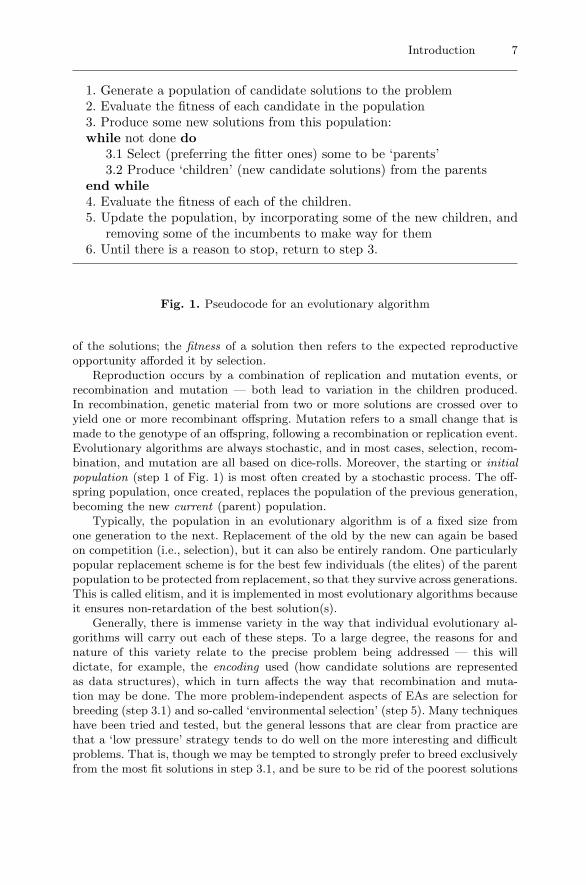
Typically, in evolutionary algorithms, there is made a distinction between thegenotype and the phenotype of a candidate solution, with the genotype being themedium of reproduction and variation (step 3.2 in Fig. 1), but with selection beingbased on the evaluation of the phenotype (steps 2 and 4). There are several alter-native schemes for selection, but the basis for them is usually a relative ranking

4 We might say there is panmictic (all-mixing) evolution.

Introduction 7

1. Generate a population of candidate solutions to the problem2. Evaluate the fitness of each candidate in the population3. Produce some new solutions from this population:while not done do

3.1 Select (preferring the fitter ones) some to be ‘parents’3.2 Produce ‘children’ (new candidate solutions) from the parents

end while4. Evaluate the fitness of each of the children.5. Update the population, by incorporating some of the new children, and

removing some of the incumbents to make way for them6. Until there is a reason to stop, return to step 3.

Fig. 1. Pseudocode for an evolutionary algorithm

of the solutions; the fitness of a solution then refers to the expected reproductiveopportunity afforded it by selection.

Reproduction occurs by a combination of replication and mutation events, orrecombination and mutation — both lead to variation in the children produced.In recombination, genetic material from two or more solutions are crossed over toyield one or more recombinant offspring. Mutation refers to a small change that ismade to the genotype of an offspring, following a recombination or replication event.Evolutionary algorithms are always stochastic, and in most cases, selection, recom-bination, and mutation are all based on dice-rolls. Moreover, the starting or initialpopulation (step 1 of Fig. 1) is most often created by a stochastic process. The off-spring population, once created, replaces the population of the previous generation,becoming the new current (parent) population.

Typically, the population in an evolutionary algorithm is of a fixed size fromone generation to the next. Replacement of the old by the new can again be basedon competition (i.e., selection), but it can also be entirely random. One particularlypopular replacement scheme is for the best few individuals (the elites) of the parentpopulation to be protected from replacement, so that they survive across generations.This is called elitism, and it is implemented in most evolutionary algorithms becauseit ensures non-retardation of the best solution(s).

Generally, there is immense variety in the way that individual evolutionary al-gorithms will carry out each of these steps. To a large degree, the reasons for andnature of this variety relate to the precise problem being addressed — this willdictate, for example, the encoding used (how candidate solutions are representedas data structures), which in turn affects the way that recombination and muta-tion may be done. The more problem-independent aspects of EAs are selection forbreeding (step 3.1) and so-called ‘environmental selection’ (step 5). Many techniqueshave been tried and tested, but the general lessons that are clear from practice arethat a ‘low pressure’ strategy tends to do well on the more interesting and difficultproblems. That is, though we may be tempted to strongly prefer to breed exclusivelyfrom the most fit solutions in step 3.1, and be sure to be rid of the poorest solutions

8 Knowles et al.

in step 5, it turns out that we get more capable and reliable algorithms when weensure that these steps are gently influenced by fitness.

Why EC works, and the benefits of EC

Evolutionary computation is very successful, but why? There is continued debateabout what underpins its general degree of success, but we first need to clarify whatwe mean by ‘success’ in order to address this question properly. What appears tobe the case, at least for some important problems, is as follows:

Performance For some problems, EC is capable of much better solutions (andachieved in better, or reasonable, time) than all or most other known meth-ods.

Sufficiency For some problems, EC is capable of solutions competitive with solutionsachieved by all or most other known methods.

Applicability EC is applicable to almost any optimization problem.Accessibility For some problems, EC has been applied, and works fine, but no com-

parisons with other methods have been done.Opportunity For some problems, EC is the only approach that can be used with any

chance at all of success — in other words, with EC we can solve problems thatwe couldn’t solve before.

The Performance statement is what most people would assume is meant by “ECis successful”. Indeed it is true, but it must be stressed that this situation exists inrelatively few cases, usually those in which an EC practitioner has worked hard inconfiguring the key components of the method – the encoding, the operators, andperhaps other features (such as using a heuristic to provide seed solutions in theinitial population). The reason for EC’s success in such cases is tied up in the factthat EC provides a framework within which a new approach can be engineered. Atheart, it seems plausible that the use of the central evolutionary concepts (Darwinianselection from a population, coupled with a means of variation) is a key element inthe success here — i.e., it is a fundamentally powerful all-purpose landscape searchstrategy. However, it is worth noting that much work (usually) needed to be doneto craft the landscape, turning it into a problem more amenable to this strategy.

The Sufficiency point is true for a great many problems, and it doesn’t seem tocharacterize EC in a particularly exciting light, yet it speaks to EC’s ‘dependability’.The key point here is that the ‘other’ methods tend to have a much larger variance intheir success than EC. Given, for example, a set of 100 different real-world problemsto solve, an EC approach, crafted with no undue effort in each case, will probably doat least ‘OK’ on each of them. In contrast, an alternative method such as Simplex,that does well in a few cases, may be inapplicable for all other cases; a graph-based search technique that does well on a certain problem may perform terriblyin other cases, and so on. Sometimes, use of EC may be over the top, like usingan electron microscope to read the small-print in an insurance policy, and a rivaltechnique will do just as well in far less time. However, that rival may have abysmalperformance elsewhere in this set of problems. And so it goes on. As we noted withregard to Performance, it seems safe to attribute the success of EC to the notionthat the Darwinian principles of evolution comprise a good all-purpose strategy fornavigating the kinds of landscapes that spring up once we start to solve a real-world problem. The style of success inherent in Sufficiency, adds some weight to

Introduction 9

this. We can understand the high variance in the performance of other methods inthis context, by suggesting that such an alternative method will be ideally tunedto aspects of the landscape structure of some (maybe very few) problems, whilebeing a manifestly hopeless strategy for other problems. The well-known gradient-descent approach is an obvious example. Essentially, with gradient-descent search,your problem will be solved quickly and optimally if the landscape’s structure is thatof a single, smooth multidimensional bowl (the optimum being the lowest point inthe centre of the bowl); but on almost any other landscape this strategy will missthe optimum, by perhaps a great distance.

Bearing much relation to the last point, the Applicability of EC is well-known,and this, in its own right, is a type of success that EC enjoys in abundance. Almostby definition, if we have an optimization problem to solve, then we already have tohand some notion of candidate structures for X and f . We need very little more thanthat before we are then able to at least make a first attempt at using EC to solvethat problem. By contrast, other optimization techniques may require additionalelements that are either unforthcoming, or painful to arrange — such as necessaryfeatures of the differentiability of f , or a sensible way to assess the quality of partialsolutions, or a requirement that candidate solutions be real-valued vectors of a fixedlength. An additional feature of EC’s general applicability, important to some, isthe great ease with which EC can exploit parallel computing resources.

Riding on its ready applicability, combined with its essential simplicity (requiringno particular mathematical or programming prowess, for example), EC is successfulpartly through its Accessibility. This in itself has led to many applications in whichEC has been used, pronounced ‘good’, ‘fine’ (or whatever), but not actually eval-uated in comparison with any alternative approaches. That is, some practitioners,given some problem that they needed to solve, have chosen EC (for one or moreof the reasons already discussed), used it, and left it at that. Such cases are validexamples of ‘EC successes’, and some are in commercial use, but that is not to saythat some alternative method wouldn’t be (perhaps much) faster, and/or producehigher-quality solutions.

So, many of the applications of EC that we see in the literature, or even in thepopular press, may only provide evidence that EC is a highly accessible algorithm,rather than contribute to the evidence that it is the best choice for the problem athan. Nevertheless there is ample evidence that for many important problems it isindeed an appropriate choice; while, in some cases it is arguably the only choice.The fact that EC imposes no constraint at all on the nature of the structures inX, the set of candidate solutions, leads to some notable achievements for EC whenresearchers exploit the Opportunity this provides. Essentially, there is no candidatein the list of (non-EC) potential methods for optimization that is able to be appliedto the problem of finding ideal strategies for a fighter pilot to use during a dogfight.However, EC has been used for this, with notable success [35]. Similarly, though onecan think of antenna design as a problem in which standard parameter vectors aremanipulated to achieve variants on standard designs, EC provides the opportunityto think of optimizing antennae in a much wider sense; thus, Lohn [23] used EC tooptimize a set of algorithms for constructing antennae (such an approach, GeneticProgramming [21], is a large subfield of EC), enabling a search through a spaceof possible antenna designs in which existing styles was just a tiny, imperceptiblecorner. In this and many other cases EC becomes a way (perhaps the only successful,and automated, way) to discover innovative solutions, rather than simply optimize

10 Knowles et al.

around standard, prior designs. Many other such examples, as well as examplesof more conventional successes, may be found on a visit to the ‘HUMIES’ awardswebsite at http://www.genetic-programming.org/hc2007/cfe2007.html

We haven’t yet quite answered the question of ‘why’ EC works. But there is nogreat mystery there. The well-known ‘No Free Lunch’ theorem [39] tells us that,given an entirely random collection of landscapes (so, think in terms of all conceiv-able landscapes) no single approach is capable of the type of success that we haveclaimed here for EC. The flip-side of this is that, given some non-random collec-tion of problems — a collection in which there is a bias towards certain elements ofgeneral structure in the problem landscapes, say — a method may well exist whichis generally better than others. It is highly plausible to suggest that the collectionof real-world problems is highly biased in such a sense. In particular, once we havegone through the process of formalising a problem sensibly, and defined X, f andthe operators we will use to move within X, landscapes that we construct are invari-ably correlated, in the sense that nearby elements of X tend to have similar cost.Thus real-world problems are highly biased towards correlated landscapes. Mean-while, the essential Darwinian strategy used by EC, which is to follow ‘clues’ in alandscape under the assumption of such correlation (apples not falling far from thetree), yet not to overcommit too soon to any particular path or region in a landscape(everyone has some chance to reproduce, rather than only the very fittest), seemswell suited to most of the landscapes in this class, while rarely being a particularlypoor approach.

The basic theory behind the EC search strategy is well known, and exemplifiedin Price’s theorem [27], which basically expresses part of the above in formal terms.In the EC field, specialisations of Price’s theorem have been derived [19], [29], [26],which express nuances of the central idea, tied to specific kinds of solution structureX. Given these highly general statements, we can be satisfied that the prowess of ECis not a magical ability, but explainable. Meanwhile, similarly general statements forseveral classes of EC algorithm enable us to be satisfied that an EA will generallymake progress in reasonable time [12, 32, 31, 37]. Beyond this, which we need not(and choose not) go into here, the EC literature is replete with incremental stepsin our understanding of the many aspects involved in how to best configure an EAfor a particular problem class. There remains very much to discover about that verypoint, but one key theme, which we certainly will develop further here, is one whichalso further evidences EC’s traits of Applicability and Opportunity. Sometimes, withother optimization methods, a problem with two or more objectives can only beaddressed if it is first simplified to a single-objective (and hence, a different) problem.But, as we will see, this hurdle is not present with EC.

3 Multiobjective Optimization: Why Many Are BetterThan One

We have seen in the last section that amongst the benefits of EC is its general appli-cability in optimization. Yet, an optimization problem defined by a single objectivefunction is itself a restricted class of problems. More generally, an optimizationproblem may have multiple objectives.

Introduction 11

A multiobjective optimization problem (MOP) is typically formalized like this:

minimize {f1(x), f2(x), f3(x), . . . , fk(x)}subject to x ∈ X

(2)

expressing the fact that we want, ideally, a single solution x that minimizes each ofk distinct cost functions (also called objective functions). These functions may wellbe conflicting to various degrees, in the sense that a solution a for which f1(a) isparticularly good, may be such that f2(a) is particularly bad.

At this point, some terminology is necessary. A solution structure x ∈ X isoften called a decision vector (and X is called the decision space), since the valuesin x tend to encapsulate the design decisions that we need to make. Meanwhile,the vector (f1(x), f2(x), ..., fk(x)) is referred to as the vector of objectives, whichinhabits the so-called objective space, typically but not necessarily �k.

The quality of a candidate solution x is now no longer measured as a scalar, butas a vector. This makes necessary a new way to assess whether or not some solutionx is better than some other solution y. Previously we might say either “x is betterthan (worse than) y” or “x and y are equally fit”. Now, we can still say that they areequally fit, to describe cases in which the objective vectors for x and y are identical,but there are two distinct ways in which x and y’s performance on the task maybe different. First, we might have “x is better than y”, as before, to cover cases inwhich x’s objective vector is better than y’s in at least one objective, and no worsein all the others. This is called dominance and we say that x dominates y. Secondly,we may have a case in which x is better than y on some objectives, but y is betterthan x on other objectives. In this situation we say that x and y are incomparable,or we say that they are nondominated.

Given a set of multiobjective solutions (such as the current population of solu-tions during an EMO algorithm run), some of this set will be dominated by othersin this set. Those that are not dominated by any others in that set (which maybe a single solution, or the whole set) form what we call the Pareto set. In objec-tive space, the set of objective vectors corresponding to the Pareto set is called thePareto front.

Commonly, the true, optimal solution to a real multiobjective problem is sucha set, containing more than one, and perhaps hundreds or thousands, of nondomi-nated points. Put another way, no single solution in X dominates (or is equal to)all other solutions in X; instead, the minimization task is satisfied by a set of dis-tinct, nondominated solutions. Strictly speaking, this set is the Pareto set (and thecorresponding objective vectors are the Pareto front), while all other sets of nondom-inated solutions that we may form from elements of x (such as the nondominatedpoints of the current population during an EMO run) are, at best, ‘approximations’to the Pareto set. Commonly, however, papers in the field refer to “Pareto front ofthe current population”, and the precise meaning is usually clear from the context.

Any single point on the Pareto front is called Pareto optimal ; it is (usually)not optimal in the single-objective sense, since it (usually) does not minimize eachof the objectives; however, it represents a compromise, such that if any solutionexists that improves upon it on one objective, then that solution will be worseon at least one other objective. Clearly, the Pareto set for any problem contains,for each objective, a point that ‘truly’ minimizes that objective. That is, if we aretrying to find a bridge design that has minimal mass, minimal cost, and whoseconstruction would involve a minimal carbon footprint, then we can expect three

12 Knowles et al.

of the solutions in the Pareto set to be, respectively, the best possible solutionsin these respects among those members of X that are feasible bridge designs. Itis almost always too much to expect, of course, that any single solution will doparticularly well on any pair of objectives, or all three at once, especially wherethere is such obvious conflict. For example, cheaper designs will invariably use lessoptimal materials in terms of strength/mass ratio, and will typically exploit mass-produced, environmentally questionable sources. Nevertheless, the vector of scoresfor these three points on each objective, representing the best attainable for eachobjective, is itself a useful reference point in multiobjective optimization, knownas the ideal point. Some multiobjective optimization methods use an estimation ofthis point in order to set target directions for the search. Similarly, the so-callednadir point represents the vector of worst values for each objective, for points in thePareto front (note that, for a problem whose Pareto front shrinks to a single point,the ideal and nadir points are the same).

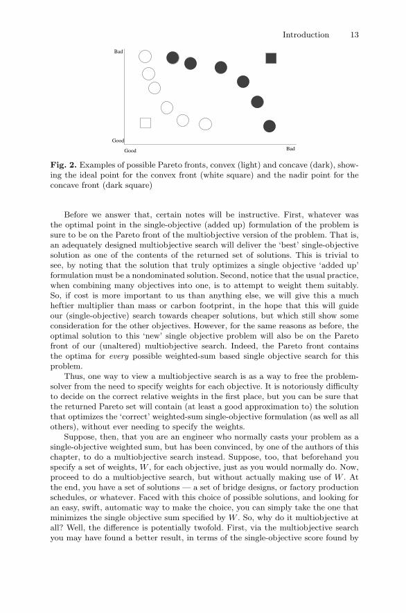
These concepts are illustrated very simply in Fig. 2, where we see contrived ex-amples of Pareto fronts for two problems. The white circles are supposed to representthe Pareto optimal solutions, plotted in objective space, for a two-objective mini-mization problem. The circles correspond to actual points (designs, decision vectors,etc.) in the Pareto set. The white square locates the ideal point — a solution that wecannot actually achieve in this problem, but showing the best attainable result foreach objective individually. Notice that this particular Pareto front ‘bulges’ towardsits ideal point — this is called a convex front. More generally, convexity is present ina Pareto front if we can generally draw straight lines between two different solutions,and find that there are solutions on the Pareto front that dominate the points onthe line. Alternatively, fronts in some problems may display much concavity — thisis the case with the Pareto front represented by black circles in Fig. 2 (these are alsoused in the figure to illustrate the concept of a nadir point). A particularly interest-ing aspect of problems with concavities in the Pareto front is that the solutions inthe concavity are not the optima of any simple weighted sum of the objectives. Thatis, these may be points that the decision maker (see later in this section) will choose,since they may form an ideal trade-off given various considerations. However, theywill invariably be missed in a search based on a single objective weighted sum, since,on such a unidimensional view of fitness, these so-called unsupported solutions arebested by other points on the front.

Now, from the viewpoint of the ‘owner’ of the optimization problem we are tryingto solve, we seem to have a difficulty. In the more common approach to optimization,we will typically combine our different objectives into one (for example, adding upa bridge design’s scores for cost, mass and carbon footprint) and concentrate onminimizing their sum. This eventually yields a single result – which is the bridgedesign that achieved the best combined score. Alternatively we may find severalsolutions that achieve the same best score, but, when using single objective methods,these will invariably turn out to be quite similar, and effectively the same design.Hence, the problem has been defined, the optimization has been done, and we canprovide the solution, and move on to the next job. However, if we treat this asa multiobjective problem, and perform a multiobjective search, our tactics for theend game are not immediately clear. The outcome of our search is now a set ofsolutions, and these will typically contain quite a variety of different designs. Whatdo we deliver as the single best design?

Introduction 13

Good

Bad

Good Bad

Fig. 2. Examples of possible Pareto fronts, convex (light) and concave (dark), show-ing the ideal point for the convex front (white square) and the nadir point for theconcave front (dark square)

Before we answer that, certain notes will be instructive. First, whatever wasthe optimal point in the single-objective (added up) formulation of the problem issure to be on the Pareto front of the multiobjective version of the problem. That is,an adequately designed multiobjective search will deliver the ‘best’ single-objectivesolution as one of the contents of the returned set of solutions. This is trivial tosee, by noting that the solution that truly optimizes a single objective ‘added up’formulation must be a nondominated solution. Second, notice that the usual practice,when combining many objectives into one, is to attempt to weight them suitably.So, if cost is more important to us than anything else, we will give this a muchheftier multiplier than mass or carbon footprint, in the hope that this will guideour (single-objective) search towards cheaper solutions, but which still show someconsideration for the other objectives. However, for the same reasons as before, theoptimal solution to this ‘new’ single objective problem will also be on the Paretofront of our (unaltered) multiobjective search. Indeed, the Pareto front containsthe optima for every possible weighted-sum based single objective search for thisproblem.

Thus, one way to view a multiobjective search is as a way to free the problem-solver from the need to specify weights for each objective. It is notoriously difficultyto decide on the correct relative weights in the first place, but you can be sure thatthe returned Pareto set will contain (at least a good approximation to) the solutionthat optimizes the ‘correct’ weighted-sum single-objective formulation (as well as allothers), without ever needing to specify the weights.

Suppose, then, that you are an engineer who normally casts your problem as asingle-objective weighted sum, but has been convinced, by one of the authors of thischapter, to do a multiobjective search instead. Suppose, too, that beforehand youspecify a set of weights, W , for each objective, just as you would normally do. Now,proceed to do a multiobjective search, but without actually making use of W . Atthe end, you have a set of solutions — a set of bridge designs, or factory productionschedules, or whatever. Faced with this choice of possible solutions, and looking foran easy, swift, automatic way to make the choice, you can simply take the one thatminimizes the single objective sum specified by W . So, why do it multiobjective atall? Well, the difference is potentially twofold. First, via the multiobjective searchyou may have found a better result, in terms of the single-objective score found by

14 Knowles et al.

W , than you would have using a single-objective search method. This is a commonlyobserved phenomenon. Second, you are presented with a diverse set of solutions thatprovides information about the trade-offs available to you. Even though the weightset W may represent for you a robust statement of what you require in a design(though usually it doesn’t), some solutions on the Pareto front that don’t optimizethis particular weighted sum may nevertheless grab your attention. You may welldiscover, for example, that an unexpectedly good saving in mass may be possiblefor just a slight increase in cost. True, what we are suggesting here is that a decisionneeds to be made, and in that sense the multiobjective search seems not to haveautomatically solved your problem for you. But, on anything more than cursoryinspection, it becomes clear that the multiobjective search has provided everythingthat the single-objective search would have provided for you, plus more, so this isnot an extra decision to be begrudged, it is an extra opportunity, to grasp or ignoreas you see fit.

Multiobjective search is therefore viewed as a way of providing the opportu-nity for a decision maker to make informed decisions about the solution based oninformation about the solutions that inhabit the Pareto front. In contrast, a single-objective formulation and search, when applied to an inherently multiobjective prob-lem, provides a solution that may look appealing in the absence of alternatives, butis otherwise potentially far from what the decision maker may choose given a bettersupply of possibilities.

When we therefore decide to face a multiobjective problem on its own terms,and apply a search method that supplies a variety of different but equally ‘optimal’solutions for a decision maker to consider, there are various ways we can respond tothis opportunity. As noted above, if we have a preferred weight vector at hand, wecan use that to pick the ‘best’ one. If instead we are skeptical about this, or any,weight vector, other approaches are available to us, from the long-established fieldof multicriterion decision making.

3.1 A Note on Multicriterion Decision Making

The man who, though exceedingly hungry and thirsty, [is] both equally,being equidistant from food and drink, is therefore bound to stay wherehe is.

Aristotle, On the Heavens (Book II)

Given that we have used an approach that generates an approximation to thePareto front, the decision maker is provided with this as both a collection of differentsolutions to the problem, and a source of information about the conflicts between theobjectives, and other aspects of the space of possible solutions. If the decision makeris an expert in the problem domain (which should normally be the case!), she maygo into a dark room, and emerge some time later having made her choice, based onperhaps deep consideration of the information at hand as well as other, unformalized(maybe unformalizable) aspects of the probable performance characteristics of thevarious potential solutions.

But, such decision makers are expensive, and it is therefore desirable to havemore formal, automated ways to help decision makers minimize their effort. These

Introduction 15

are generally ways to use additional information about the problem or problemdomain, which may have been difficult to include in the original search that led tothe Pareto set. There are many standard such methods, and the reader may refer toany textbook on multicriterion decision making for further information on the manyexisting techniques for selecting a final preferred solution (e.g see [10, 25, 34, 38]).

To provide a flavour of the type of method in use, however, we mention first theidea of ‘preference articulation’. When an expert is at hand who is able to provideauthoritative views on how to balance conflicting measures and goals, this can beexploited by using preference articulation techniques [8, 2, 20], whereby a series ofconcrete questions about preferences are asked to the decision maker. The answersthen determine if it is possible to build one or other type of consistent model ofthe decision maker’s internal utility function; if so, then an automated procedurecan potentially be developed for solution evaluation/selection. Note that far morecomplicated types of model exist for this than a simple weighted sum over theobjectives.

3.2 Visualization Methods

When tackling an optimization problem, visualization may be used to present vari-ous features revealed about the problem, or to present information about the searchmethod being used. Amongst other things, the purposes of visualization include es-timating the optimal solution value, monitoring the progress or convergence of anoptimization run, assessing the relative performance of different optimizers (includ-ing stochastic optimizers whose results form a distribution), and surveying featuresof the search landscape.

In multiobjective optimization, the above purposes of visualization remain im-portant, but the set-valued nature of the results and the conflicts that exist betweenobjectives mean that additional or dual aspects come into play. These will ofteninclude gaining an appreciation of the location and range of the Pareto set/front,assessing conflicts and trade-offs between objectives, and selecting preferred solu-tions.

In the following, we briefly present some of the visualization techniques used bycontributors in this book. For more information on visualization techniques that gobeyond those used in this book, the reader is referred to [25] (pp. 239–249), [28]and [24].

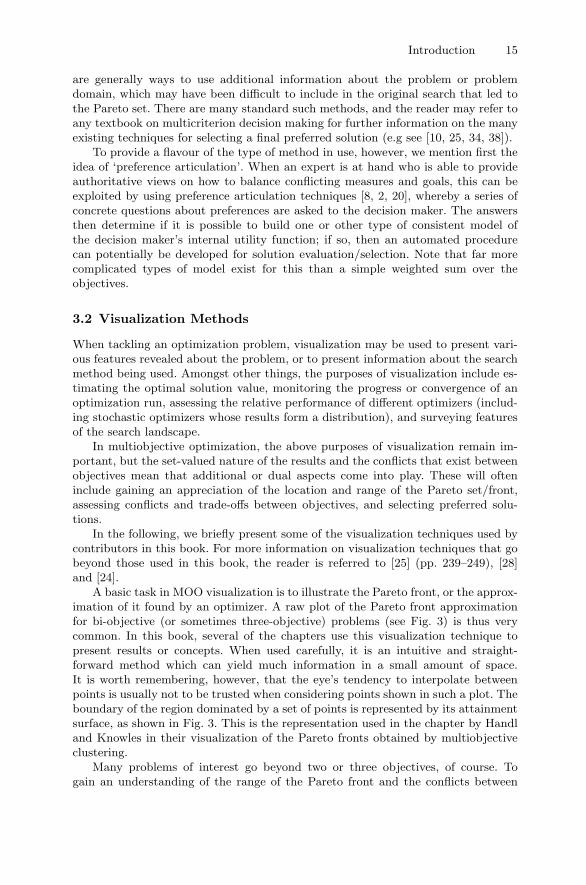
A basic task in MOO visualization is to illustrate the Pareto front, or the approx-imation of it found by an optimizer. A raw plot of the Pareto front approximationfor bi-objective (or sometimes three-objective) problems (see Fig. 3) is thus verycommon. In this book, several of the chapters use this visualization technique topresent results or concepts. When used carefully, it is an intuitive and straight-forward method which can yield much information in a small amount of space.It is worth remembering, however, that the eye’s tendency to interpolate betweenpoints is usually not to be trusted when considering points shown in such a plot. Theboundary of the region dominated by a set of points is represented by its attainmentsurface, as shown in Fig. 3. This is the representation used in the chapter by Handland Knowles in their visualization of the Pareto fronts obtained by multiobjectiveclustering.

Many problems of interest go beyond two or three objectives, of course. Togain an understanding of the range of the Pareto front and the conflicts between

16 Knowles et al.

0

5

10

15

20

25

30

0 5 10 15 20 25 30

min

imiz

e f2

(x)

minimize f1(x)

0

5

10

15

20

25

30

0 5 10 15 20 25 30

min

imiz

e f2

(x)

minimize f1(x)

Fig. 3. (Top) A standard two-objective plot of a Pareto front approximation. (Bot-tom) The corresponding attainment surface represents the family of tightest goalsthat are known to be attainable as a result of the points found

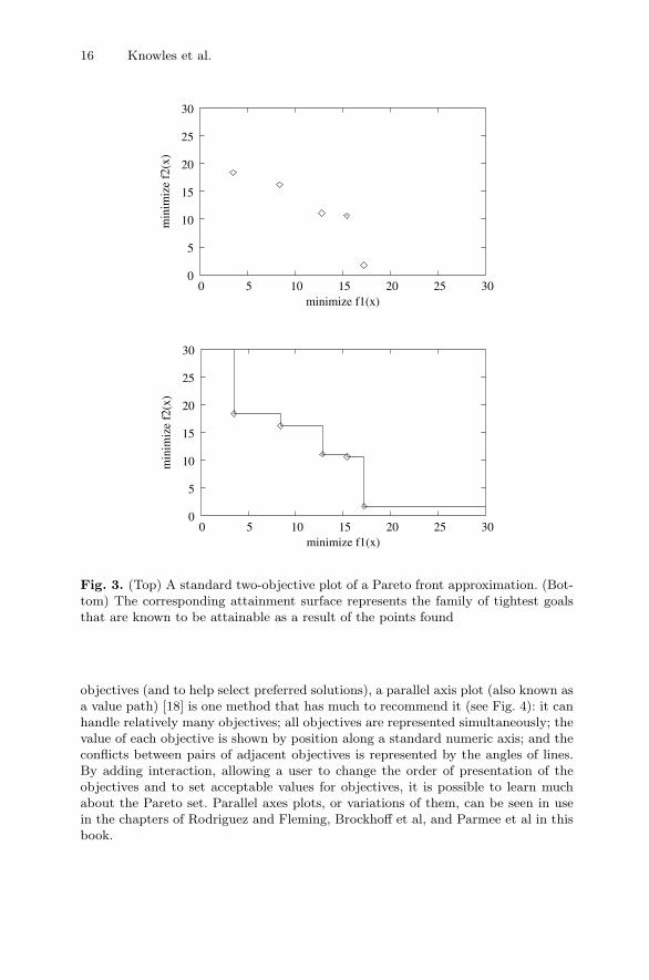
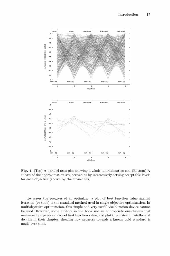
objectives (and to help select preferred solutions), a parallel axis plot (also known asa value path) [18] is one method that has much to recommend it (see Fig. 4): it canhandle relatively many objectives; all objectives are represented simultaneously; thevalue of each objective is shown by position along a standard numeric axis; and theconflicts between pairs of adjacent objectives is represented by the angles of lines.By adding interaction, allowing a user to change the order of presentation of theobjectives and to set acceptable values for objectives, it is possible to learn muchabout the Pareto set. Parallel axes plots, or variations of them, can be seen in usein the chapters of Rodriguez and Fleming, Brockhoff et al, and Parmee et al in thisbook.

Introduction 17

0

0.1

0.2

0.3

0.4

0.5

0.6

0.7

0.8

0.9

1

1 2 3 4 5

norm

aliz

ed fi

tnes

s (m

in is

bet

ter)

objectives

max=1 max=1 max=0.98 max=0.99 max=0.99

min=-8.8 min=-8.9 min=-8.7 min=-8.9 min=-8.6

0

0.1

0.2

0.3

0.4

0.5

0.6

0.7

0.8

0.9

1

1 2 3 4 5

norm

aliz

ed fi

tnes

s (m

in is

bet

ter)

objectives

max=1 max=1 max=0.98 max=0.99 max=0.99

min=-8.8 min=-8.9 min=-8.7 min=-8.9 min=-8.6

Fig. 4. (Top) A parallel axes plot showing a whole approximation set. (Bottom) Asubset of the approximation set, arrived at by interactively setting acceptable levelsfor each objective (shown by the cross-hairs)

To assess the progress of an optimizer, a plot of best function value againstiteration (or time) is the standard method used in single-objective optimization. Inmultiobjective optimization, this simple and very useful visualization device cannotbe used. However, some authors in the book use an appropriate one-dimensionalmeasure of progress in place of best function value, and plot this instead. Cutello et aldo this in their chapter, showing how progress towards a known gold standard ismade over time.

18 Knowles et al.

Similarly, it is often useful in single-objective evaluation to plot best functionvalue achieved (after convergence) against some metaparameter, like a parameterof the search method used. Jin et al and Branke et al in this volume both plotone-dimensional performance metrics against meta-parameters to show the effectsof the latter on search performance.

3.3 From EAs to EMOAs

Our primary interest in this book is the use of evolutionary multiobjective optimiza-tion algorithms (EMOAs) — that is, evolutionary algorithms that work directly withfitness vectors, rather than scalar fitness values. The benefits and merits of EAs, asdiscussed above, carry over directly to EMOAs, while the steps we need to take tooperate with fitness vectors rather than scalars are relatively straightforward, as weshall briefly discuss.

Before launching into an introduction to EMOAs, however, we do not dismissalternative optimization strategies. Though not our focus, non-EMOA multiobjec-tive optimization predates EMOA, and continues to thrive. The field of operationsresearch (OR) is the primary alternative to EMO in this respect.

OR boasts a rich and growing multiobjective optimization literature. Many ofthe problems considered in OR are multiobjective versions of convex problems, e.g.,minimum spanning tree, where the single-objective version is polynomial-time solv-able by convex optimization methods; to find Pareto optima of the multiobjectiveproblem, one can scalarize the objectives, and apply the same convex methods (sofinding one Pareto optimum is ‘easy’). However, for most of these problems, it canbe shown that the number of Pareto optima is exponential in the number of inputvariables, and hence finding the Pareto optimal set is intractable for large problems(see [11]). For these reasons, some of the work reported in the OR literature is basedon mathematical programming techniques supplemented with different schemes forapproximately sampling the Pareto front via scalarizing methods. Methods alsobased on traditional optimization techniques, but using decision-making before orinteractively during optimization to reduce the number of Pareto optima to find,are also popular.

In parallel, the OR field has also developed methods for nonconvex multiob-jective optimization problems. These rely mainly on approximate optimization al-gorithms such as simulated annealing and tabu search. To adapt them for use inmultiobjective optimization, two main approaches are possible. One is to adjust thecore functions of the algorithm, such as the acceptance function, so as to base deci-sions on dominance relations between solutions (or other factors, such as proximityof solutions in objective space). The other is to leave the basic algorithm in itsoriginal form, and rely on scalarizing techniques (as used in the mathematical pro-gramming approaches discussed above) to build up an approximation of the Paretooptimal front.

Meanwhile, in recent years, some OR researchers have begun to experiment withevolutionary algorithm approaches, encouraged by the rapid development of the fieldof evolutionary multiobjective optimization. This brings us to our main topic.

There are comprehensive and authoritative recent texts available providing re-views of and descriptions of the field of EMO (e.g., [5, 15, 7]). The central differenceto the single objective case is the assignment of fitness — obviously, each individual

Introduction 19

in the population now has its performance characterized by a fitness vector, ratherthan a single value. Perusal of Fig. 1 suggests that the only way this need affect theoperation of an evolutionary algorithm is in the selection steps — i.e., steps 5 and9, in which we are making decisions that require us to compare candidate solutionsin terms of relative fitness. This is indeed the case, and EMO algorithms tend to becharacterized by how these steps are performed.

The primary style of approach, often referred to (see several of the coming chap-ters) as Pareto ranking, is to give each point in the population a single score based onthe degree to which it dominates, or is dominated by, other points in the population.In one of the most celebrated such approaches, nondominated sorting [36], the scoreassigned to a candidate solution reflects the ‘depth’ to which it dominates othercandidates in the current population. Specifically, all of the nondominated solutionsin the population are given the best rank (say, rank 1). These are then marked as‘ranked’, and we proceed to find the nondominated front among the unranked re-mainder. These are ranked 2, and the process continues until all candidates havebeen ranked. An individual’s rank is then converted into a selective probability inany one of numerous ways. Often, for example, practitioners will borrow the simpleTournament Selection method common in single objective EAs, in which some (usu-ally) small number from the population are randomly picked, and the best of these(highest ranked, breaking ties randomly) becomes selected as a parent. As for theother selection step (step 5 in Fig. 1), the typical approach in EMOAs is to ensurethat the Pareto front of the merged parent and child population is preserved, andany remaining space in the population is filled by relatively highly ranked members.It is common, however, for the Pareto front size to be larger than the populationsize — when this happens (and more generally too, e.g., in considering which ofthe non-front candidates to keep, when this is an issue) — selection decisions areoften based on density in objective space. So, we might prefer to maintain pointsthat are in relatively sparsely populated parts of the front, and don’t mind losingsolutions that are in crowded sections. These are certainly not the only approachesto selection, and meanwhile we have skipped over many issues that are the topicof hot research subareas in the field. However, the reader is again referred to anyof several accessible papers and texts that present the main techniques, and othersthat describe ongoing research areas.

Meanwhile, the remainder of the book attempts to characterize and focus on acertain category of subareas, in which EMO is considered more widely, as a frame-work in which a variety of novel approaches to problem solving can be devised andimplemented.

4 New Directions in Problem Solving with MOOTechniques

Rather than regarding problems as immutably divided into single-objective andmultiobjective, and basing such distinctions purely on the properties required ofa solution to the problem, EMO scientists, in practice, are finding reasons to blurthese distinctions, co-opting the EMO mechanisms for handling individual objectivesfor related but distinct purposes that enhance the optimization process. This bookis largely about the most prominent and successful of these new problem-solving

20 Knowles et al.

approaches. It is not a book of EC techniques or of isolated applications, but ratherconcentrates on the concepts guiding the use of EMO in broad problem classes. Inparticular, it shows how EMO

• can be used to understand and resolve ill-defined problems;• helps in dynamic optimization environments, in problems with constraints, and

in various learning problems where quality is not always directly measurable orfree from biases;

• can eliminate a measurement bias or other confounding factor in the optimizationof an objective;

• can combine information from multiple sources;• can change the landscape of a problem, making it easier to search;• supports proper progress and convergence in search problems where the objective

is not explicit, but instead based on tests or competitions (e.g., in co-evolution);• and, may be employed in the reverse-engineering of artificial and natural systems,

where it can contribute to the quest for new principles of design.

Among these and other lessons, we also learn more about the decision-making stepfor choosing a ‘final’ solution that is associated with more traditional uses of mul-tiobjective optimization, and explore how this need not be an entirely subjectivematter. In some uses of EMO presented in this book — for example, when apply-ing it to traditional ‘single-objective’ problems, like constrained optimization — the‘best’ solution is not a function of decision-maker preferences, and its identificationcan be automated.

4.1 Chapter Summaries

Part I — Exploiting Multiple Objectives: From Problems toSolutions

Part I of the book is a collection of chapters about problem formulation. It showshow broad classes of problem, usually formulated with a single objective to optimize,can be re-cast as multiobjective problems, with various beneficial and sometimeseven dramatic effects. In some cases, the effect achieved is an improvement in theefficiency of searching the problem space. In other cases, there is a more profoundeffect, so that different and better solutions can be accessed asymptotically, i.e., theultimate potential outcome of the search is improved. In yet other cases, the newproblem formulation yields a greater understanding of a problem, with its competinggoals and objectives, and this can help to re-evaluate the problem, possibly leadingto a more conscious refinement of it.

Using several objectives to help solve what are traditionally considered ‘single-objective’ problems may raise the spectre of ‘relaxing’ the problem in some people’sminds, resulting in a set of trade-offs, when only one solution is really wanted.However, as is shown throughout the chapters in Part I, this does not turn outto be a difficulty: the single-objective formulation (if it exists in well-defined form)can always be invoked post hoc to select the best solution; and where this is foundinappropriate, it is because the multiobjective problem formulation has revealed aweakness, or a hidden assumption, in the original problem definition — one thatshould be externalized and dealt with appropriately. This issue of selecting the finalsolution is discussed at some level in most of these chapters, and what is found is

Introduction 21

an interesting contrast to the usual view that multiobjective optimization alwaysimplies a phase of (human) decision making.

Ficici (Chap. 2) considers co-evolutionary algorithms (CEAs), a thriving areaof research that has the potential to make valuable contributions to the breadth ofthe whole problem-solving domain. The defining characteristic of CEAs is that thefitness of an individual (a candidate solution) is defined, implicitly, by interactionswith other individuals. From this, it follows that CEAs can be used to solve prob-lems for which no known (explicit) objective function exists: problems that would beimpossible to tackle using traditional optimization methods, such as finding optimalstrategies in two- or multi-player games. Ficici’s chapter shows how Pareto optimal-ity can be used as an organizing principle in CEAs, with each individual being viewedas a potential objective for optimization. From this idea, several long-standing dif-ficulties associated with CEAs can be better understood and largely circumvented.Moreover, the multiobjective framework allows the general co-evolutionary learningproblem to be handled in such a way that monotonic improvement of solutions isensured. This idea relates to elitism in MOEAs, and to the use of archives of non-dominated solutions, a theme which is touched on in several other chapters in thebook, particularly de Jong and Bucci’s. The issue of decision making is raised inthe chapter, and its relationship to the concept of refinement, and the equilibriumselection problem in game theory is described, with some tantalizing prospects forfuture developments.

One of the earliest uses of multiobjective methods for solving single-objectiveproblems was their application in constrained optimization, an area thoroughly re-viewed in Mezura-Montes and Coello’s work (Chap. 3). Constrained optimizationproblems represent a large and important chunk of real-world problems, especiallyin engineering, but they still pose a challenge to traditional evolutionary algorithmmethods. In this chapter, the common EA approach of using penalty functions iscompared, conceptually, with multiobjective formulations of the problem. Two ben-efits of the latter are posited: that weights do not have to be selected in order tobalance the different importance or ranges of the constraints; and, that the numberof improving paths to the optimum is much greater, which increases the possibility ofapproaching good solutions. Work that both supports and criticizes these assertionsis considered, and an empirical study is used to compare some of the current state-of-the-art methods. In constrained optimization, it is shown that decision makingnever enters as a matter of DM preferences, even in the multiobjective formulation.In other words, there is an automatic way of selecting the objectively best solutionfrom the Pareto front in all cases.

Another considerable area of research in problem solving concerns optimizationin dynamically changing contexts, as explained in Chap. 4., Bui et al. investigateusing a secondary helper objective for this class of problems, aimed at maintainingdiversity in the evolving population, and thus a readiness for sudden or periodicchanges in the optima. The use of a secondary objective, and application of standardMOEAs, is a simple approach to handling dynamism, and what is more it does notintroduce any issues related to decision making. Comparisons made with existing EAmechanisms for dynamic problems, namely hypermutation and random immigration,show the MOEA approach already gives the most consistently good performance,while there remains much room for further development of the technique.

Cutello et al (Chap. 5) apply multiobjective EAs to the traditionally single-objective problem of predicting a protein’s native structure, a pressing and massively

22 Knowles et al.

significant problem in the biological sciences. The rather specialized nature of thisproblem belies the fact that it may serve as an archetype for others in which theobjective function is not really objective or final, but a proxy used to help findsolutions. In structure prediction, it is an energy function that is minimized, and thisis essentially a guess made up of several components of energy; the ultimate arbiterof quality, however, is not the objective function, but the distance to the observed,real structure (which is not available at the time of optimization in real instances ofthe problem, however). Taking a multiobjective approach to the problem (here bydecomposing the energy function into its components) is a process of learning howto align the objective functions with the ultimate measure of solution quality. Here,the flexible nature of multiobjective search is being used as a way to improve themodels on which the optimization is based.

Neumann and Wegener’s interest (Chap. 6) is in the possibility that for well-defined problems a multiobjective formulation could be straightforwardly faster tosolve for an evolutionary algorithm than a single-objective one. Taking two classicproblems from combinatorial optimization, the single source shortest path problemand the minimum spanning tree problem, they demonstrate that this possibility isnot a fiction. For the MST, the asymptotic expected optimization time is derivedfor simple multiobjective and single-objective EAs, indicating the superiority of theformer. Experimental results on different instance types also show a performanceadvantage of multiobjective algorithms for some classes of minimum spanning tree.In all cases, the problem formulations used here directly yield unique solutions tothe original problem and no extra step of decision making is involved.

Handl and Knowles (Chap. 7) express and develop a view of problem-solving-via-MOO that concords with some of the ideas expressed in the preceding five chapters.They believe that in practical problem-solving applications, MOO is used in a va-riety of subtly different ways, called modes. The modes capture the specific reasonwhy the problem has been formulated with multiple objectives, and what job eachof the objectives is doing. Handl and Knowles identify five different modes and pro-vide examples of each from their own research. They also show how some modesrequire no decision making for solution selection, while others reveal useful trade-off information that would normally be hidden, but which must be accounted forto select a final operational solution. For the latter case, however, some automaticand semi-automatic methods of decision making have been successfully devised, no-tably those based on the shape of the Pareto front and the consideration of controldistributions.

Part II — Multiple Objectives in Machine Learning

Part II of the book concerns the application of MOO to different problems in machinelearning. The chapters collected here, like those in part I, emphasise the reasoningbehind the multiobjective formulations presented, and demonstrate that core diffi-culties in machine learning can be understood and alleviated by the multiobjectiveapproach. Common themes in machine learning, and in these chapters, are the trade-off between accuracy and model complexity; conflicts between training, validationand testing errors; and the combining of rules or classifiers. More unusual issuesthat are also highlighted include competing errors in multi-class problems, programbloat in genetic programming, and the value of promoting models that humans canunderstand in system identification.

Introduction 23

Fieldsend et al (Chap. 8) consider the supervised learning paradigm, in whichthe output class or value of a datum must be predicted from its inputs, following aperiod of training on a random i.i.d. sample of example data. It is well known that thesupervised learning problem is about generalization performance, which is difficult toassess during training, and hence different terms are often added to the basic trainingerror objective to achieve regularization or model selection. Fieldsend et al considermultiobjective approaches to this central issue, and show some graphical methods foridentifying solutions that best balance accuracy vs model complexity. The chapteralso identifies a number of supervised learning problems where competing error termsare inherent, and a balance must be struck between them. One such is the differentcosts of misclassifications in multi-class data, most notably in disease diagnosis.Some groundbreaking methods in this problem area are presented.

The first of two consecutive chapters on genetic programming is Bleuler et al’s(Chap. 9). Genetic programming is a form of computer program induction, basedon evolutionary algorithm principles (see [22]). Bleuler et al focus on the problemof ‘bloat’ in GP, whereby evolved programs have the tendency to grow larger andlarger, containing more and more useless code. This problem with GP has beena bugbear for several years, and several methods for counteracting it have beenproposed and studied. In recent years, several multiobjective approaches have beentried, with considerable success. In this chapter, the reason behind the success ofthe Pareto-based approach to reducing bloat is investigated, following a thoroughreview of this area.

Rodriguez-Vazquez and Fleming (Chap. 10) concentrate on the use of geneticprogramming in system identification, specifically for non-linear dynamical systems.They show how a multi-stage process, which involves going back and forth betweensteps of structure selection, parameter estimation and validation can be compressedinto a one-step process through the use of a multiobjective formulation. Moreover,human understanding of generated models is identified as an important issue whichcan be further enhanced by including objectives that control the type and complexityof model components used.

Rule mining is a method of classification, often for large databases, based ontwo processes, (i) extracting useful rules and (ii) combining them. Ishibuchi et al(Chap. 11) investigate both processes, exploring what is meant by a Pareto optimalrule and a Pareto optimal rule set, and how these can be approximated. They uncoverinteresting relations between accuracy and complexity, which echo the ‘switchbackeffect’ shown in Fieldsend et al’s earlier chapter. They also show that Pareto optimalrule sets are not necessarily comprised entirely of Pareto optimal rules, and this ismore the case as the ruleset size is allowed to grow.

Part III — Multiple Objectives in Design and Engineering

In design and engineering, it is quite widely understood and accepted that problemsinvariably have competing objectives, and that problem solving is about finding goodbalances, or spotting niches where a different type of solution might be attractivefor the first time. Part III of the book is about this area, particularly open-endeddesign, where it is almost a given that problems are multiobjective, when viewed atsome level. Instead of explaining why and how multiple objectives arise here, thechapters rather focus on how to support understanding, learning and invention ina multiobjective space, and also how the same principles that are used for design

24 Knowles et al.

might also help when analysing and seeking to understand existing natural systems,which have inevitably evolved under several and various selection pressures.

Deb and Srinivasan (Chap. 11) suggest a systematic procedure of using two ormore conflicting objectives (usually minimization of size and maximization of per-formance) to unveil salient knowledge about properties which when present in asolution would make it an optimal solution corresponding to the underlying objec-tives. The argument works as follows. Since Pareto-optimal solutions are no ordinarysolutions in the search space, but rather correspond to optimal solutions of certaintrade-offs among objectives, a series of such solutions is expected to possess somecommon properties that can provide a practitioner with important knowledge about‘what makes a solution optimal?’. This process of ‘innovization’ — the creation ofinnovative knowledge through multiobjective optimization — is illustrated througha number of engineering design problems.

Parmee’s focus (Chap. 12) is on methods to support the human designer as shegoes about her business, particularly in the area of conceptual design. Advancedmethods of visualization, interactive evolution and machine learning are described,all aimed at taking away the drudgery of evaluation, and freeing the designer to makemore insightful and high-level choices and inferences, based on an understanding ofthe multiobjective nature of the problem space.

Moshaiov is interested in analogies that can be drawn between artificial andnatural systems (Chap. 13). He explores how and why such analogies have beenuseful because of what they can tell us about the design process, and about natural(evolved) phenomena. From this historic background, he moves on to consider why,in cybernetics, artificial life and evolutionary biology, the concept of trade-off isknown, but a multiobjective view is rarely taken. Moshaiov explains how such aview could be made acceptable to both biologists and engineers, and considers whatthe consequences of this broader outlook might be.

Part IV — Scaling Up Multiobjective Optimization

Much evidence for the potential of multiobjective optimization to deliver new andpowerful solutions to problems, from classic combinatorial optimization problemsto open-ended design problems, is provided in the first three parts of the book. Toturn this into a reality, there is, of course, a continuing need for the development ofeffective multiobjective optimization methods. Of great concern to the field in recenttimes has been the scalability of the algorithms and concepts we use — scalabilityto increasing numbers of objectives and to larger design spaces. Part IV of the bookpresents some of the latest developments in the design of scalable multiobjectiveevolutionary algorithms.

Jin et al (Chap. 15) consider how the relatively low-dimensional manifold inwhich Pareto optimal solutions reside can be modeled and projected back into themuch higher dimensional parameter space. Such an approach promises to achievegreat scalability in parameter space dimension, provided certain base assumptionsare valid. Jin et al show excellent performance of their techniques for problems withup to 100 real-valued parameters.

The first of three chapters concerned with methods capable of handling problemswith many objectives is provided by Hughes (Chap. 16). He provides a backgroundto the issue and reviews the capabilities of several existing Pareto and non-Pareto

Introduction 25

multiobjective EAs at handling problems with four or more objectives. He considersboth the issues of convergence to the Pareto front, and of controlling the distributionof points along it.

De Jong and Bucci (Chap. 17) are concerned with a particular class of problemsthat results in optimization problems with many objectives, easily tens or hundredsof them. This class is where the objectives are defined in terms of ‘tests’, an approachthat may be taken when other methods of evaluation are not possible. Although thespace of tests is usually very large, de Jong and Bucci show that tests need not all bearranged on orthogonal axes, but they can be grouped together, depending on howthey affect the ordering of candidate solutions. This enables a significant reductionin the number of effective objective dimensions considerably.

Brockhoff et al (Chap. 18) also seek to reduce the number of objectives pre-sented, to a lower number, which is easier to handle effectively. The first methodfor doing this has similarities with de Jong and Bucci’s method for tests: it dependson inspection of the orderings induced by the objectives on sampled sets of solu-tions, and whether or not these orderings can be preserved when some objectivesare removed from consideration. The second method does not consider orderings perse, it is based on principal components analysis on the objectives to establish theredundant ones. Both techniques are demonstrated on test instances, and unifyingconcepts are discussed.

5 Concluding Remarks

There are many interesting topics vying for inclusion in a book on multiobjectiveproblem solving. Our choice has been guided by the desire to present the emergingconcepts and methods that are being used to tackle important and long-standingclasses of problems; and as a result some things have necessarily been left out. Wehave not touched on the use of other natural analogies in multiobjective problemsolving, such as methods based on social insect behaviour, or flocking — methodsthat can trump evolutionary algorithms in some domains. We have not consideredmultiobjective optimization for problems where the number of solution evaluationspossible is severely restricted, an area which is gaining rapid prominence because ofthe take-up of EMO in engineering and science, where evaluations are often costly.In machine learning, we covered several topics, but left out the contribution MOOis beginning to make in searching for ensembles of neural networks [4], though en-sembles of rules are considered in the chapter by Ishibuchi et al.

And you, the reader, may well consider that we have overlooked something else— and you are surely right. But what remains in the book is, we hope, the beginningsof a synthesis that shows the contributions MOO is making to the core activity ofproblem solving with computers. Rather than an esoteric technique at the fringes ofevolutionary algorithm research, or a specialist’s area in operations research, MOOis now being used to help people solve all sorts of problems by offering genuinelynew approaches to them. It goes beyond a method that allows engineers to balanceout different criteria — though that is an important aspect of it. It can transforma problem, reaching solutions that were not possible before, or allowing monotonicprogression where cycling previously occurred. It can take us to solutions, even toclassic problems, more quickly than before. And we have seen that the algorithms

26 Knowles et al.

for achieving this are being developed anew, with fresh concepts to take us on to anew scale of problem-solving ability.

Acknowledgment

JK gratefully acknowledges the support of the Biotechnology and Biological SciencesResearch Council (BBSRC), UK.

References

[1] N. A. Barricelli. Numerical testing of evolution theories Part II: Preliminarytests of performance, symbiogenesis and terrestrial life. Acta Biotheoretica,16(3–4):99–126, 1963.

[2] V. Belton and T. J. Stewart. Multiple Criteria Decision Analysis: an IntegratedApproach. Springer-Verlag, Berlin, Germany, 2002.

[3] H. J. Bremermann. Optimization through evolution and recombination. InSelf-Organizing Systems, pages 93–106. Spartan Books, Washington, DC, 1962.

[4] A. Chandra and X. Yao. Ensemble Learning Using Multi-Objective Evolution-ary Algorithms. Journal of Mathematical Modelling and Algorithms, 5(4):417–445, 2006.

[5] C. A. Coello Coello, D. A. Van Veldhuizen, and G. B. Lamont. EvolutionaryAlgorithms for Solving Multi-Objective Problems. Kluwer Academic Publishers,New York, May 2002. ISBN 0-3064-6762-3.

[6] D. Corne, K. Deb, P. Fleming, and J. Knowles. The Good of the Many Out-weighs the Good of the One: Evolutionary Multi-Objective Optimization. IEEEConnections Newsletter, 1(1):9–13, 2003.

[7] K. Deb. Evolutionary Algorithms for Multi-Criterion Optimization in Engi-neering Design. In K. Miettinen, M. M. Makela, P. Neittaanmaki, and J. Pe-riaux, editors, Evolutionary Algorithms in Engineering and Computer Science,chapter 8, pages 135–161. John Wiley & Sons, Ltd, Chichester, UK, 1999.

[8] J. S. Dyer, P. C. Fishburn, R. E. Steuer, J. Wallenius, and S. Zionts. Multi-ple criteria decision making, multiattribute utility theory: the next ten years.Management Science, 38(5):645–654, 1992.

[9] G. Dyson. Darwin Among the Machines. Penguin Books, 1999.[10] M. Ehrgott. Multicriteria Optimization. Number 491 in Lecture Notes in

Economics and Mathematical Systems. Springer, Berlin, 2000.[11] M. Ehrgott and X. Gandibleux. An Annotated Bibliography of Multi-objective

Combinatorial Optimization. Technical Report 62/2000, Fachbereich Mathe-matik, Universitat Kaiserslautern, Kaiserslautern, Germany, 2000.

[12] D. Fogel. Asymptotic convergence properties of genetic algorithms and evo-lutionary programming: Analysis and experiments. Cybernetics and Systems,25(3):389–407, 1994.

[13] D. B. Fogel. An introduction to simulated evolutionary optimization. IEEETransactions on Neural Networks, 5(1):3–14, 1994.

[14] L. J. Fogel. Autonomous automata. Industrial Research, 4(1):14–19, 1962.

Introduction 27

[15] C. M. Fonseca and P. J. Fleming. An Overview of Evolutionary Algorithmsin Multiobjective Optimization. Evolutionary Computation, 3(1):1–16, Spring1995.

[16] A. S. Fraser. Simulation of genetic systems by automatic digital computers.Australian Journal of Biological Sciences, 10:484–491, 1957.

[17] M. R. Garey and D. S. Johnson. Computers and Intractability: A Guide to theTheory of NP Completeness. W. H. Freeman and Company, San Francisco,1979.

[18] A. M. Geoffrion, J. S. Dyer, and A. Feinberg. An Interactive Approach forMulti-Criterion Optimization, with an Application to the Operation of an Aca-demic Department. Management Science, 19(4):357–368, 1972.

[19] J. H. Holland. Adaption in Natural and Artificial Systems. University of Michi-gan Press, 1975.

[20] R. L. Keeney and H. Raiffa. Decisions with Multiple Objectives: Preferencesand Value Trade-Offs. Cambridge University Press, Cambridge, UK, 1993.

[21] J. R. Koza. Genetic Programming: On the Programming of Computers by Meansof Natural Selection. MIT Press, 1992.

[22] W. B. Langdon and R. Poli. Foundations of Genetic Programming. Springer,2002.

[23] J. Lohn, G. Hornby, and D. Linden. An Evolved Antenna for Deployment onNASA’s Space Technology 5 Mission. In Genetic Programming Theory andPractice II, pages 13–15. Springer, 2004.

[24] A. V. Lotov, V. A. Bushenkov, and G. K. Kamenev. Interactive Decision Maps:Approximation and Visualization of Pareto Frontier. Kluwer Academic, 2004.

[25] K. Miettinen. Nonlinear Multiobjective Optimization. Kluwer Academic Pub-lishers, 1999.

[26] R. Poli and W. Langdon. Schema Theory for Genetic Programming with One-Point Crossover and Point Mutation. Evolutionary Computation, 6(3):231–252,1998.

[27] G. R. Price. Selection and covariance. Nature, 227:520–521, 1970.[28] A. Pryke, S. Mostaghim, and A. Nazemi. Heatmap visualization of population

based multi objective algorithms. In Evolutionary Multi-Criterion Optimization(EMO 2006), volume 4403 of LNCS, pages 361–375. Springer, 2006.

[29] N. Radcliffe. The algebra of genetic algorithms. Annals of Mathematics andArtificial Intelligence, 10(4):339–384, 1994.

[30] I. Rechenberg. Cybernetic solution path of an experimental problem, 1965.Library Translation 1122, Royal Aircraft Establishment, Farnborough, UK.

[31] G. Rudolph. Convergence analysis of canonical genetic algorithms. IEEE Trans-actions on Neural Networks, 5(1):96–101, 1994.

[32] G. Rudolph. Convergence of evolutionary algorithms in general search spaces.In Proceedings of the IEEE International Conference on Evolutionary Compu-tation, pages 50–54, 1996.

[33] H.-P. Schwefel. Kybernetische Evolution als Strategie der experimentellenForschung in der Stromungstechnik. Master’s thesis, Hermann Fottinger Insti-tute for Hydrodynamics, Technical University of Berlin, 1965.

[34] Y. Siskos and A. Spyridakos. Intelligent multicriteria decision support:Overview and perspectives. European Journal of Operational Research,113(2):236–246, 1999.

28 Knowles et al.

[35] R. E. Smith, B. A. Dike, B. Ravichandran, A. El-Fallah, and R. Mehra. Discov-ering Novel Fighter Combat Maneuvers in Simulation: Simulating Test PilotCreativity. In Creative Evolutionary Systems, pages 467–486. Morgan Kauf-mann, 2001.

[36] N. Srinivas and K. Deb. Multiobjective optimization using nondominated sort-ing in genetic algorithms. Technical report, Department of Mechanical Engi-neering, Indian Institute of Technology, Kanpur, India, 1993.

[37] D. Thierens and D. Goldberg. Convergence models of genetic algorithm selec-tion schemes. In Parallel Problem Solving from Nature — PPSN III, volume866 of LNCS, pages 119–129, 1994.

[38] P. Vincke. Multicriteria Decision-aid. Wiley, New York, 1992.[39] D. H. Wolpert and W. G. Macready. No free lunch theorems for optimization.

IEEE Transactions on Evolutionary Computation, 1:67–82, 1997.