Pontifícia Universidade Católica

do Rio de Janeiro

Arthur Amorim Bragança

Three Essays on Rural Development in Brazil

Tese de Doutorado

Thesis presented to the Postgraduate Program in Economics of the Departamento de Economia, PUC-Rio as a partial fulfillment of the requirements for the degree of Doutor em Economia

Advisor: Prof. Juliano Assunção Co-advisor: Prof. Claudio Ferraz

Rio de Janeiro

August 2014

Pontifícia Universidade Católica

do Rio de Janeiro

Arthur Amorim Bragança

Three Essays on Rural Development in Brazil

Thesis presented to the Postgraduate Program in Economics of the Departamento de Economia, PUC-Rio as partial fulfillment of the requirements for the degree of Doutor em Economia. Approved by the following comission:

Prof. Juliano Assunção Advisor

Departamento de Economia - PUC-Rio

Prof. Claudio Ferraz Co-advisor

Departamento de Economia - PUC-Rio

Prof. Gustavo Gonzaga Departamento de Economia - PUC-Rio

Prof. Leonardo Rezende Departamento de Economia - PUC-Rio

Prof. Bernardo Mueller Departamento de Economia - UnB

Prof. Rodrigo Soares EESP/FGV

Prof. Mônica Herz Coordinator of the Centro de Ciências Sociais - PUC-Rio

Rio de Janeiro, August 18, 2014

All rights reserved.

Arthur Amorim Bragança

Arthur Bragança holds a B.A. in Economics from the

Federal University of Minas Gerais (UFMG) and a Ph.D.

in Economics from the Catholic University of Rio de

Janeiro (PUC-Rio). During his Ph.D. studies, he was a

visiting scholar in the Department of Economics at Harvard

University for a period of one year. The primary focus of

his research has been development, agriculture,

environmental and resource economics, and political

economics.

Bibliographic Data

Bragança, Arthur Amorim

Three Essays in Rural Development in Brazil / Arthur Amorim Bragança; advisor: Juliano Assunção; co-advisor: Claudio Ferraz – 2014

155 f. : il. (color.); 30 cm

Tese (Doutorado em Economia) - Pontifícia Universidade Católica do Rio de Janeiro, Rio de Janeiro, 2014.

Inclui bibliografia.

1. Economia – Teses. 2. Desenvolvimento Rural. 3. Mudança Tecnológica. 4. Adoção de Tecnologia. 5. Migração. 6. Economia Política. 7. Desmatamento. I. Assunção, Juliano. II. Ferraz, Claudio. III. Pontifícia Universidade Católica do Rio de Janeiro, Departamento de Economia. IV. Título.

CDD: 330

Acknowledgements

Gostaria de agradecer a todos aqueles que contribuíram para minha formação

acadêmica.

Agradeço primeiramente à minha família. Aos meus pais, Jáiron e Andréia, pelo

amor, ensinamentos e apoio. À minha esposa, Laísa, pelo amor e apoio

incondicionais e essenciais para minha vida. Obrigado por ter aceitado viver todos

os desafios da vida ao meu lado. À minha irmã, Carolina, pela amizade e

companheirismo. Aos meus avós, José Edgard e Maria Helena, pelos exemplos de

vida fundamentais para minha formação. Ao meu padrinho, à minha afilhada e aos

meus demais familiares pela presença constante e pelos muitos momentos de

alegria juntos.

Agradeço também a todos os professores e funcionários do Departamento de

Economia da PUC-Rio. Sou extremamente grato ao meu orientador, Juliano

Assunção, e ao meu coorientador, Claudio Ferraz, pelas oportunidades,

ensinamentos, conselhos, confiança e generosidade. Essa tese não existiria sem o

apoio deles aos meus projetos de pesquisa. Agradeço ao Professor Marcelo de

Paiva Abreu tanto pelo exemplo profissional quanto pelas conversas sobre história

econômica que alteraram a minha trajetória acadêmica. Agradeço ao Professor

Rodrigo Soares pelos ótimos cursos e pelos ensinamentos e comentários que

muito contribuíram para minha formação profissional. Agradeço também aos

professores Leonardo Rezende e Gustavo Gonzaga, coordenadores da pós-

graduação no início e no final da minha trajetória como aluno da PUC-Rio, pelo

compromisso com a excelência do programa de pós-graduação.

Agradeço ao professor Nathan Nunn por ter viabilizado o meu doutorado

sanduíche e por ter me recebido para inúmeras conversas. A experiência na

Universidade de Harvard enriqueceu muito minha formação acadêmica e foi

fundamental para o aperfeiçoamento dessa tese.

Meu muito obrigado também aos meus amigos da PUC-Rio, do CPI, de Harvard,

da UFMG e do Colégio Santo Antônio. Agradeço aos amigos da PUC-Rio,

Fernando, Adão e Breno, pela amizade e aprendizado ao longo do mestrado e

doutorado. Agradeço aos amigos do CPI, Dimitri, Pedro e Romero, pela constante

troca de ideias sobre economia, agricultura e desmatamento. Agradeço aos amigos

da UFMG, Fabrício, Júlio, João, Tinoco e Fred, pelo companheirismo e momentos

de alegria. Agradeço às amigas da UFMG, Marina, Cristina, Patrícia e Fernanda,

pela amizade, torcida e apoio. Agradeço também ao Juan, ao Bernard e ao

Ricardo, amigos economistas que me acompanham desde os tempos de colégio.

Por último, agradeço o apoio financeiro da CAPES, do CNPq e do Climate Policy

Initiative (CPI) que viabilizaram esse trabalho e o auxílio de toda equipe do CPI

na montagem dos dados geográficos e socioeconômicos utilizados nessa tese.

Abstract

Bragança, Arthur; Assunção, Juliano (advisor); Ferraz, Claudio (co-

advisor). Three Essays on Rural Development in Brazil. Rio de Janeiro,

2014. 155p. Tese de Doutorado – Departamento de Economia, Pontifícia

Universidade Católica do Rio de Janeiro.

This thesis is composed of three articles on rural development in Brazil. The

first article studies the impact on labor selection of the technological innovations

implemented in the 1970s that allowed soybean cultivation in Central Brazil. It

combines the timing of these innovations with variation on agronomic potential to

cultivate the crop to evaluate the effect of the technological innovations. Results

indicate that the innovations changes agricultural practices with increases in the

use of modern inputs. The changes in agricultural practices affected the demand

for skill in agriculture and induced selection into agriculture of individuals with

higher educational attainment and selection out of agriculture of individuals with

lower educational attainment. Suggestive evidence indicates that the impact of the

technological innovations on output would be one third lower in the absence of

labor selection. The second article examines whether geographic heterogeneity

affects technology adoption. We develop a simple model in which geographic

heterogeneity affects adoption by influencing adaptation costs. The model predicts

the impact of geographic heterogeneity on technology adoption to be negative and

non-monotonic. We test the model predictions using data on soil heterogeneity

and the adoption of the Direct Planting System in Brazil. This technology

increases revenues and decreases costs and its adoption neither requires large

costs nor increases risk. However, the direct planting system must be adapted to

specific site conditions, making adoption costly when geographic heterogeneity is

large. We use detailed data on soil characteristics to show that geographic

heterogeneity negatively impacts adoption in a pattern consistent to the theoretical

model. The results indicate that geographic heterogeneity can be an important

barrier to the diffusion of agricultural technologies. The third article studies the

connection between special interests and government policies in the context of

conservation policies in the Brazilian Amazon. Industries like agriculture or

logging often oppose stringent conservation policies and the paper examines

whether these industries are able to influence conservation policies. I construct a

measure of connection to agricultural interests of the local politicians and use a

regression discontinuity design to provide evidence that municipalities with

mayors connected to agriculture have higher deforestation rates in election years.

The timing of the effect indicates that special interests (as opposed to ideological

preferences) drive the result. Estimates also suggest that the effect is higher when

the politicians have reelection incentives and is related to changes in enforcement

of environmental regulations. The results provide evidence that politicians distort

policies near elections to benefit special interest groups connected to them. The

first article is co-authored with Juliano Assunção and Claudio Ferraz while the

second article is co-authored with Juliano Assunção and Pedro Hemsley.

Keywords

Agricultural Development; Technological Change; Technology Adoption;

Migration; Political Economics; Deforestation

Resumo

Bragança, Arthur; Assunção, Juliano (orientador); Ferraz, Claudio

(coorientador). Three Essays on Rural Development in Brazil. Rio de

Janeiro, 2014. 155p. Tese de Doutorado – Departamento de Economia,

Pontifícia Universidade Católica do Rio de Janeiro.

Essa tese é composta de três artigos sobre desenvolvimento rural no Brasil.

O primeiro artigo analisa o impacto das inovações tecnológicas que, na década de

1970, adaptaram a soja para o Brasil Central sobre seleção de trabalhadores. O

artigo combina o momento das inovações tecnológicas com variação agronômica

no potencial para cultivo de soja para estimar os efeitos dessas inovações. Os

resultados indicam que as inovações tecnológicas ocasionaram mudanças nas

práticas agrícolas com aumento do uso de insumos modernos. Essas mudanças nas

práticas agrícolas afetaram a demanda por capital humano e induziram imigração

de trabalhadores qualificados e emigração de trabalhadores desqualificados. A

evidência também sugere que o impacto das inovações tecnológicas sobre a

produção agrícola seria um terço menor na ausência de fluxos de trabalhadores. O

segundo artigo examina se heterogeneidade geográfica afeta adoção de tecnologia.

O artigo desenvolve um modelo teórico simples em que heterogeneidade

geográfica afeta adoção de novas práticas através de sua influência sobre custos

de adaptação. O modelo prediz uma relação negativa e não monotônica entre

heterogeneidade geográfica e adoção de tecnologia. Essa predição é testada

utilizando dados de heterogeneidade de solos e adoção do Plantio Direto na Palha

na agricultura brasileira. Essa tecnologia aumenta lucros e sua adoção não requer

investimentos fixos e não aumenta riscos. Todavia, o Plantio Direto na Palha

precisa ser adaptado para condições locais, tornando sua adoção custosa quando a

heterogeneidade dos solos é alta. Os resultados empíricos mostram que a

heterogeneidade de solos reduz adoção do Plantio Direto na Palha de maneira

consistente com o modelo teórico. Essa evidência sugere que heterogeneidade

geográfica pode ser uma importante barreira para a difusão de práticas agrícolas

modernas. O terceiro artigo analisa a relação entre grupos de interesse e políticas

públicas no contexto de políticas de combate ao desmatamento na Amazônia

brasileira. Representantes da agropecuária e da indústria madeireira se opõem a

essas políticas devido ao seu efeito negativo sobre suas atividades e o artigo

investiga se esses grupos de interesse utilizam seu poder político para influenciar

políticas de combate ao desmatamento. O artigo constrói uma medida de conexão

dos políticos aos interesses da agropecuária e utiliza um desenho de regressão

com descontinuidade para mostrar que municípios governados por políticos

ligados à agropecuária apresentam maior taxa de desmatamento em anos

eleitorais. Os resultados também sugerem que o efeito é mais forte em municípios

onde o prefeito tem incentivos de reeleição e está conectado a mudanças na

fiscalização ambiental. Essa evidência indica que políticos distorcem políticas

públicas para beneficiar grupos de interesse conectados a eles. O primeiro artigo é

co-autorado com Juliano Assunção e Claudio Ferraz e o segundo com Juliano

Assunção e Pedro Hemsley.

Palavras-chave

Desenvolvimento Rural; Mudança Tecnológica; Adoção de Tecnologia;

Migração; Economia Política; Desmatamento

Contents

1 Technological Change and Labor Selection in Agriculture: Evidence from the

Brazilian Soybean Revolution 13

1.1. Introduction 13

1.2. Historical Background 17

1.3. Data 22

1.4. Identification Strategy 26

1.5. Technological Change and Agricultural Modernization 29

1.6. Technological Change and Labor Selection 34

1.7. Robustness Checks 40

1.8. Conclusion 43

2 Geographic Heterogeneity and Technology Adoption: Evidence from the Direct

Planting System 61

2.1. Introduction 61

2.2. Historical Background 66

2.3. Model 70

2.4. Data 75

2.5. Soil Heterogeneity and Technology Adoption 78

2.6. Is the Impact of Soil Heterogeneity Non-Monotonic? 87

2.7. Conclusion 89

3 Special Interests and Government Policies: The Impact of Farmer Politicians on

Deforestation in the Brazilian Amazon 102

3.1. Introduction 102

3.2. Institutional Background 106

3.3. Data and Sample Selection 111

3.4. Identification Strategy 115

3.5. Results 119

3.6. Mechanism: Enforcement or Demand for Deforestation? 126

3.7. Conclusion 128

References 142

List of Tables

Table 1.1: Descriptive Statistics – Agricultural Censuses ..................................... 47

Table 1.2: Descriptive Statistics - Population Censuses........................................ 48

Table 1.3: The Effect of Technological Change on Soybean Adoption ................ 49

Table 1.4 The Effect of Technological Change on Land Use ............................... 50

Table 1.5: The Effect of Technological Change on Input Use .............................. 51

Table 1.6: The Effect of Technological Change on Agricultural Output .............. 52

Table 1.7: The Effect of Technological Change on Migration ............................. 53

Table 1.8: The Effect of Technological Change on Educational Attainment ....... 54

Table 1.9: The Effect of Technological Change on Educational Attainment –

Individuals Born from 1930 to 1955 ............................................................. 55

Table 1.10: The Effect of Technological Change on Occupational Choices ........ 56

Table 1.11: Migration, Selection and Agricultural Output .................................... 57

Table 1.12: Robustness I – Checking the Parallel Trends Assumption................. 58

Table 1.13: Robustness II – Additional Controls for Agricultural Outcomes ....... 59

Table 1.14: Robustness II – Additional Controls for Population Outcomes ......... 60

Table 2.1: Costs and Benefits from the DPS ......................................................... 95

Table 2.2: Descriptive Statistics ............................................................................ 96

Table 2.3: Adoption Rates per State ...................................................................... 97

Table 2.4: OLS Regressions .................................................................................. 98

Table 2.5: Alternative Heterogeneity Measures and Alternative Samples ............ 99

Table 2.6: Land Distribution, Credit and Access to Markets .............................. 100

Table 2.7: Falsification Tests............................................................................... 101

Table 3.1: Descriptive Statistics .......................................................................... 137

Table 3.2: The Impact of Mayors Connected to Agriculture on Predetermined

Outcomes, RD Estimates ............................................................................. 138

Table 3.3: The Impact of Mayors Connected to Agriculture on Deforestation

Rates, RD Estimates .................................................................................... 139

Table 3.4: The Impact of Mayors Connected to Agriculture on Deforestation

Rates: Heterogeneous Effects ...................................................................... 140

Table 3.5: Mechanisms Linking Politicians Connected to Agriculture and

Deforestation ............................................................................................... 141

List of Figures

Figure 1.1 – Soybean Potential in Central Brazil .................................................. 45

Figure 1.2 – Technological Change and Educational Attainment across Cohorts 46

Figure 2.1: The Diffusion of the DPS in Brazil ..................................................... 91

Figure 2.2: Soil Heterogeneity and DPS Adoption at Different Quantiles ........... 92

Figure 2.3: Soil Heterogeneity and Electricity Use at Different Quantiles ........... 93

Figure 2.4: Soil Heterogeneity and Harvester Use at Different Quantiles ............ 94

Figure 3.1: Sample Municipalities ...................................................................... 129

Figure 3.2: Trends in Deforestation ..................................................................... 130

Figure 3.3: McCrary Test .................................................................................... 131

Figure 3.4: Balancing Tests – Electoral Covariates ............................................ 132

Figure 3.5: Balancing Tests – Land Use Covariates ........................................... 133

Figure 3.6: Correlations (OLS and FE) ............................................................... 134

Figure 3.7: The Impact of Farmers on Deforestation, RD Estimates .................. 135

Figure 3.8: The Impact of Farmers on Deforestation, RD Estimates .................. 136

1 Technological Change and Labor Selection in Agriculture: Evidence from the Brazilian Soybean Revolution

1.1.Introduction

Technological innovations are essential to promote agricultural

development. An extensive literature argues that improvements in crops and

fertilizers and the development of tractors and harvesters were critical to promote

agricultural growth throughout the past centuries both in developed and

developing countries.1

Adjustments to technological innovations can lead to substantial labor

reallocation to and from agriculture. The theoretical literature suggests that

technological change in agriculture can affect both the size and composition of the

agricultural labor force (Schultz, 1953; Matsuyama, 1992; Ngai and Pissarides,

2007; Lagakos and Waugh, 2013; Young, 2013). Existing empirical studies

document the effects of technological innovations on the size of the rural labor

force but are silent on the impact of these changes on the composition of the

agricultural labor force (Caselli and Coleman II, 2001; Foster and Rozenzweig,

2008; Nunn and Qian, 2011; Bustos et al., 2014; Hornbeck and Keskin,

Forthcoming). Assessing the consequences of technological innovations for labor

selection in agriculture is essential to understand the incidence of these

innovations. It is also important to explain important phenomena such as the

income differences between agricultural and non-agricultural activities (Gollin et

al., 2014).

This paper uses the historical experience from agriculture in Central Brazil

to provide causal evidence on the connection between technological innovations

and labor selection in agriculture. It explores exogenous variation coming from

technological innovations that adapted soybeans for the agro-climatic

1 See Griliches (1958), Olmstead and Rhode (2001, 2008) and Evenson and Gollin (2003) for

evidence of the importance of technological innovations to agricultural development in different

contexts.

14

characteristics from Central Brazil to understand whether it influenced the

composition of the agricultural labor force.

Soybean adaptation was the result of biological innovations implemented

during the 1970s that enabled its cultivation in Central Brazil. Technological

innovations adapted soybeans for the poor and acid soils from the region and

reshaped agriculture in this agricultural frontier. Adaptation allowed farmers to

move from extensive cattle grazing using almost no modern inputs to intensive

crop cultivation using modern inputs and machines (Klink and Moreira, 2002).

Historical accounts suggest that the shift from pasture to crop cultivation

affected human capital demand as crop cultivation is more skill-intensive than

cattle grazing.2 In particular, soybean cultivation required use of modern inputs

and experimentation with seeds and fertilizers. Historical accounts indicate that

these activities are intensive in human capital.3

We organize the analysis in two different parts. First, we investigate the

effects of the technological innovations on land use and agricultural practices in

Central Brazil. Second, we assess the impact of these innovations on migration

rates and the composition of the agricultural labor force. In particular, we

investigate whether the technological innovations affected educational attainment

both of migrants and natives to understand its impact on labor selection in

agriculture.

Our empirical design combines the timing of the technological change with

variation in agronomic potential for soybean cultivation using modern

technologies to estimate the impact of the technological innovations. Following

Nunn and Qian (2011) and Bustos et al. (2014), we use FAO/GAEZ data to

construct a measure of agronomic potential for soybean cultivation using modern

technologies.4 We use this measure to estimate whether outcomes increased faster

in municipalities with higher soybean potential when compared to municipalities

with lower soybean potential. Baseline specifications include geographic and

2 See Strauss et al. (1991) for some evidence of the importance of human capital to the

adoption of modern technologies in Central Brazil. 3 See Welch (1970) for a discussion of the importance of skills to foster experimentation in

agriculture. See also Foster and Rosenzweig (1996) for evidence on the complementarities

between modern agricultural inputs and skills. 4 Nunn and Qian (2011) are the first paper which used FAO/GAEZ data in economics while

Bustos et al. (2014) propose the measure of agronomic potential used in this paper.

15

baseline municipal characteristics as controls to mitigate the concern that

differential trends in the outcomes drive the estimates.

We document that the technological innovations had a sizable effect on land

use. Following the technological innovations, crop cultivation increased in

municipalities more suitable for soybean cultivation using modern technologies.

The increase in crop cultivation is associated with a rise in the use of modern

inputs such as liming and tractors.5 The effects on the adoption of these inputs are

substantial and point out that the technological innovations induced intensification

of the agricultural practices.

We also find that the changes in land use and agricultural practices did not

increase the use of labor in agriculture. However, the results indicate that

migration rates increased, suggesting that the technological innovations induced

significant labor movements. This reallocation affected characteristics of the

agricultural labor force as educational attainment increased both among migrants

and natives. Human capital accumulation does not explain the results as the

findings are robust to restricting the sample to cohorts outside school when the

innovations took place. These findings suggest that the technological innovations

stimulated immigration of individuals with higher-than-average human capital to

municipalities more suitable for soybean cultivation and emigration of individuals

with lower-than-average human capital from these localities. A conservative

calculation suggests that such selection pattern account for about half of the

increase in educational attainment in these municipalities.

We interpret this result as evidence that the technological innovations

increased human capital demand in agriculture. This interpretation is consistent

with the results on agricultural practices and the literature documenting that

modern technologies and human capital are complements in agriculture (Foster

and Rosenzweig, 1996). Further evidence supporting this interpretation comes

from occupational choices. Results point out that the technological innovations

increased the share of the agricultural labor working in occupations intensive in

human capital (such as driving tractors, preparing soils, applying fertilizers etc.).

5 Liming is the most important fertilizer to crop cultivation in central Brazil as it is needed to

reduce soil acidity. See Rezende (2002) for a discussion of the importance of investments in

liming to agricultural production in Central Brazil.

16

The labor movements can increase the effects of the technological

innovations on agricultural output, facilitating adjustment in land use and farming

practices.6 To provide evidence on this mechanism, we estimate the impact of the

technological innovations on agricultural output both excluding and including

measures of schooling and occupational structure as controls. The effects of the

technological innovations decrease in 30 to 35% when these covariates are

included. This result provides suggestive evidence that selection was essential to

enable agriculture to adapt and benefit from the technological innovations.

The results survive to a number of robustness exercises. We use data from

pre-treatment periods to provide evidence that the trends in agricultural outcomes

before the technological innovations were similar in municipalities with different

levels of agronomic potential. We also construct a price index to show that the

results are robust to controlling for changes in prices. We also provide evidence

that the results are robust to the inclusion controls for access to credit and land

tenure. This robustness check mitigates concerns that other policies drive the

estimates.

Our results contribute to different streams of the literature. Earlier literature

documented that technological change in agriculture affects the size of the rural

labor force (Caselli and Coleman II, 2001; Foster and Rosenzweig, 2008; Nunn

and Qian, 2011; Bustos et al., 2014; Hornbeck and Keskin, Forthcoming). We

complement this literature showing that agricultural development also affects the

composition of the rural labor force. This evidence is important to understand

different phenomena such as the income differences between agricultural and non-

agricultural activities (Lagakos and Waugh, 2013; Young, 2013; Gollin et al.,

2014). In particular, our results complement the evidence from Bustos et al.

(2014). These authors document that technological innovations in the Brazilian

agriculture are associated with labor movements from agriculture to other

industries. Our evidence uses a different historical experiment to document that

technological innovations in the Brazilian agriculture also associated with changes

in labor selection. Both studies highlight that technological innovations in

agriculture have significant consequences for labor movements.

6 Existing empirical studies suggest that farmers face difficulties to adjust agricultural

practices to different growing conditions (Olmstead and Rhode, 2008; Hornbeck, 2012; Bazzi et

al., 2014).

17

This paper also provides novel evidence on the connection between

technological innovations and educational attainment in agriculture. Foster and

Rosenzweig (1996) document that the Green Revolution increased human capital

demand in agriculture and induced its accumulation in India. The technological

innovations studied in this paper also increased the human capital demand in

agriculture. However, our results point out that labor selection explains a

substantial share of the increase in educational attainment. Hence, this paper

brings attention to the importance of migration in the adjustment to changes in

production possibilities in agriculture.

Moreover, our results contribute to the literature investigating the causes

and consequences of the expansion of the Brazilian agricultural frontier during the

last decades (Gasques et al., 2004; Rada and Buccola, 2012; Rada, 2013). It

provides causal evidence on the role of technological innovations in affecting the

composition of the labor force in the agricultural frontier.

The remaining of the paper is organized as follows. Section 2 provides

background information on technological innovations and agricultural

development in central Brazil. Section 3 describes the data. Section 4 presents the

empirical design used in the estimates. Section 5 presents the results on

agricultural outcomes. Section 6 presents the results on labor selection. Section 7

presents the robustness exercises. Section 8 concludes.

1.2. Historical Background

1.2.1. Agricultural Development in Central Brazil before 1970

Central Brazil covers about one fifth of Brazil and is composed of four

states (Goiás, Mato Grosso, Mato Grosso do Sul and Tocantins). It is mostly

located in the Cerrado biome although some of its lands are in other biomes. The

main characteristics of this biome are the prevalence of savannah vegetation and

the tropical climate with a rainy summer and a dry winter. The region's soils are

infertile due to a combination of soil acidity, aluminum prevalence, and nutrient

scarcity.7 These features limited occupation and agricultural development in

Central Brazil until recent decades. High transportation costs to the main Brazilian

cities and ports exacerbated the region's natural disadvantages and further limited

7 Detailed information on the Cerrado can be found in Oliveira and Marquis (2002).

18

its occupation and agricultural development (Guimarães e Leme, 2002; Klink and

Moreira, 2002).

Industrialization and urbanization of neighboring states increased the

demand for meat and promoted extensive cattle ranching in the region after 1920.

Cattle ranching benefited from the native pastures that cover a substantial share of

Central Brazil's land area. However, its impact on occupation and agricultural

development was limited since it used little labor or modern inputs (Klink and

Moreira, 2002).

Promoting occupation and agricultural development in the region became an

objective of several Brazilian governments after 1940 (Guimarães and Leme,

2002). The Brazilian government aimed to promote crop cultivation in central

Brazil in order to meet the growing food demand created due to a combination of

urbanization and population growth (Klink and Moreira, 2002). Expanding

agricultural production was considered important to ease the pressures on food

prices and avoid inflation.

The government also sought to expand the agricultural frontier to foster

industrialization through higher demand for farm inputs. It believed that the

expansion of the agricultural frontier would increase the demand for tractors and

fertilizers and help these industries to develop in Brazil. Finally, the expansion of

the agricultural frontier was considered important to reduce pressures on land

reform in other regions. In particular, the conservative modernization proposed

after the 1964 coup sought to relieve these pressures through population

movements to the agricultural frontier rather than through land reform (Salim,

1986; Helfand, 1999; Houtzager and Kurtz, 2000).

Incentives for agricultural production along the agricultural frontier after

1940 included both subsidies and investments in infrastructure (Klink and

Moreira, 2002). The government subsidized credit and provided agricultural credit

lines with negative interest rates. It also established minimum price programs to

reduce risks that farmers faced when operating on the agricultural frontier. In

addition, the government invested in road building and electrification.

Colonization projects concentrated subsidies and investments in

infrastructure (Santos et al., 2012). Colonization projects were either public or

private depending on the region. These projects provided farmers with land rights

and some basic infrastructure which facilitated migration and induced farmers to

19

move to the agricultural frontier (Jepson, 2002). The first colonization projects

were created in the 1940s in the municipalities of Ceres (in the state of Goiás) and

Dourados (in the state of Mato Grosso do Sul).8 Subsequent projects were

established in the region until the 1980s.

Government policies induced the occupation of Central Brazil after 1940.

Rural population increased 3% per year from less than 1 million in 1940 to 2.6

million in 1970 despite the substantial urbanization experienced during that period

in Brazil as a whole. However, the evolution of rural development was less

impressive. Income per inhabitant increased 1.7% per year in the same period.

Historical accounts emphasize that limited agricultural development was a

consequence of the increased cultivation of the region's acid and nutrient poor

soils (Sanders and Bein, 1976). Crop cultivation was an intermediate stage

between deforestation and cattle grazing since it helped the soil to retain nutrients.

For this reason, investments in fertilizers and tractors remain limited (Klink and

Moreira, 2002).

1.2.2. Technological Change and the Adaptation of Soybeans for Central Brazil

Adverse agro-climatic characteristics were an important constraint to

agricultural development in Central Brazil. These characteristics limited

cultivation of agricultural products – such as soybeans and cotton – cultivated

with success in other Brazilian regions. Government investments in agricultural

research started in the 1960s aiming to overcome the geographic constraints that

agricultural production faced in Central Brazil (Klink and Moreira, 2002). These

investments were inspired by the Green Revolution in other developing

countries.9 The adaptation of soybeans to the growing conditions found in Central

Brazil is a case of success of these public investments in agricultural research.10

Investments focused in engineering soybean varieties adapted to the tropical

climate and the Cerrado biome started in the 1950s in the Instituto Agronômico de

Campinas and expanded in the 1960s with the establishment of a national

8 The Colônia Nacional Agrícola de Goiás (CANG) was founded in Ceres in 1942 while the

Colônia Nacional Agrícola de Dourados (CAND) was founded in 1944. 9 Cabral (2005) describes the importance of the Green Revolution in other developing

countries in inducing the Brazilian government to invest in agricultural research. 10

It is unclear in the literature what motivated the Brazilian government to invest in soybean

research and not in other crops.

20

program that coordinated and promoted research on this crop. These investments

continued to increase fast in the subsequent decade with the creation of Embrapa,

the national agricultural research corporation (Spehar, 1994; Cabral, 2005; Kiihl

and Calvo, 2008).

Soybean adaptation was essential for its cultivation in Central Brazil. Yields

from traditional varieties in Central Brazil were lower than 1 ton per hectare

(compared to yields higher than 2 tons per hectare in southern Brazil). The central

issue to plant development in the region was the reduced sunlight exposition in

tropical areas compared to temperate areas from which the crop originates.

Another important issue was the abundance of aluminum, which is toxic to plants,

in the region's soils (Spehar 1994). Both issues impaired plant development and

negatively affected the yields obtained using traditional varieties.

The investments in soybean research succeeded both in developing varieties

resistant to aluminum and adapted to the tropical climate. Varieties adapted to the

agro-climatic characteristics from Central Brazil were developed following the

experiences of the Green Revolution elsewhere. The first varieties that could be

cultivated in some Central Brazil areas were launched in 1965 and 1967. These

varieties were adapted to latitudes lower than 20 degrees, enabling soybean

cultivation in southern localities of the region along the states of Goiás and Mato

Grosso do Sul. These varieties achieved experimental yields higher than 2 tons per

hectare. Varieties more resistant to aluminum were developed in 1969 and 1973.

A significant development came in 1975 with the development of the Cristalina

cultivar, which achieved experimental yields higher than 3 tons per hectare and

could be cultivated in more localities from Central Brazil. Later developments

generated in Embrapa research centers created varieties quite resistant to high

aluminum levels and adapted to latitudes below 10 degrees (Spehar, 1994; de

Almeida et al., 1999). These developments complete the adaptation process.

1.2.3. Agricultural Development in Central Brazil after 1970

Historical accounts suggest that the technological innovations led to a

considerable expansion of soybean cultivation in Central Brazil after 1970 (Klink

and Moreira, 2002). Cultivation at the beginning of the 1970s was concentrated in

the region's southernmost areas as the varieties introduced in the late 1960s could

not be cultivated in latitudes smaller than 10 degrees. Technological developments

21

induced settlement and cultivation in northern Central Brazil by the end of the

1970s despite the reduction in international prices.11

Soybean cultivated area

reached more than 2.5 million hectares in 1985. Yields more than doubled in the

period.

The expansion of soybean cultivation induced substantial changes in

agricultural practices. Rezende (2002) argues that technological innovations were

essential to turn intensive agriculture viable in Central Brazil. Nevertheless, the

author also argues that the expansion of crop cultivation also required significant

investments in land preparation as liming and other fertilizers must be used in

large amounts to fertilize soils. His calculation indicates that expenditures with

liming and other fertilizers represent 42.5% of the total investments needed to

prepare land for intensive agriculture. As a comparison, land acquisition

represents 25% while land clearing represents 17.5% of these investments.

Investments in tractors are also required to intensive agriculture in Central

Brazil. The prolonged droughts common in the region turn the use animal traction

impossible as soils become too compact during the dry season (Sanders and Bein,

1976). Plowing using animal traction must begin after the end of this season. Such

timing reduces water absorption as soils are still compact when it starts raining. It

also pushes plowing to a period when mules and other animals are debilitated.

Tractors remove these constraints with farmers being able to prepare soils during

the drought. Technical assistance also became more important as farmers must

experiment with distinct crop varieties never tested in that environment (Jepson,

2006a, b).

The changes in agricultural practices needed to soybean cultivation seem to

have increased human capital demand and induced migration. The literature

suggests that migration was important to promote the adoption of modern

agricultural technologies in Central Brazil (Kiihl and Calvo, 2008). Migrants

benefited from previous experience with crop agriculture and modern farming

inputs (de Carli, 2005; Monteiro et al., 2012). Settlement was concentrated in

areas in which government investments and public or private colonization projects

had provided land rights and some infrastructure (Jepson, 2002; Santos et al.,

11

The increase in international prices increased soybean cultivation in the 1970s in subtropical

areas as well. However, cultivated area remained constant in these areas following the fall in prices

in the second half of the decade while it continued to expand in Central Brazil.

22

2012). Settlers started cultivating rice as aluminum-resistant varieties were

available (Monteiro et al., 2012). Soybean cultivation started later as farmers

needed time to experiment with different varieties (Macêdo, 1998; Jepson, 2006a,

b). Existing research suggest that human capital was critical to induce

experimentation and soybean adoption (Strauss et al., 1991).

1.3. Data

1.3.1. Data on Soybean Potential

Evaluating the impact of technological innovations in agriculture is often

difficult since the time series correlation between innovations and agricultural

outcomes might be spurious and capture unobserved determinants of these

variables. For this reason, it is important to build a credible empirical design to

investigate the effects of the technological innovations that adapted soybeans to

Central Brazil.

Our empirical design explores variation in the municipalities that benefited

more from the technological innovations to investigate its effect on agricultural

and socioeconomic outcomes. We measure the gain from the technological

innovations with data from the Food and Agriculture Organization (FAO) Global

Agro-Ecological Zones (GAEZ) database. The database uses an agronomic model

that combines geographical and climatic information to predict potential yields for

several crops under different levels of input use. Levels of input use range from

low (corresponding to traditional agricultural practices) to high (corresponding to

commercial agriculture using machinery and chemicals). The data is reported in

0.5 degrees by 0.5 degrees grid cells.12

Following Bustos et al. (2014), we define the agronomic potential for

cultivating soybeans using modern technologies as the difference between the

potential soybean yield under the high and the low input level. The measure

captures the potential gain that a farmer could obtain shifting land use to soybean

12

The FAO/GAEZ dataset was introduced in the economics literature by Nunn and Qian

(2011) who investigate the effect of the introduction of potatoes in urbanization in Europe. This

dataset was subsequently used in a number of papers such as Costinot et al. (Forthcoming) who

investigate the impact of climate change in agriculture, Bustos et al. (2014) who investigate the

impact of Genetically Engineered (GE) crops on agriculture and industrialization in Brazil and

Marden (2013) who investigate the impact of agricultural reforms on agriculture and

industrialization in China.

23

after its adaptation to Central Brazil. A limitation of the measure used is that the

agronomic model that underlies the FAO/GAEZ data uses contemporaneous (as

opposed to historical) information on technologies to measure agricultural

potential for each crop. Hence, we are assuming that technological change after

the period analyzed did not change the comparative advantage to cultivate

soybeans across Central Brazil.13

This restrictive assumption can be validated

using data on soybean adoption. We should not observe a positive correlation

between soybean adoption and agronomic potential if technological change after

the sample period affected comparative advantage. We return to this issue in the

discussion of the results.

We measure soybean potential measure at the municipality level that is the

administrative division for which data on the Agricultural Census is available. It is

also the smallest administrative division for which we observe the location of

individuals in the Population Census. Several municipalities were created in the

region and some other municipalities change their borders in the period analyzed.

We account for this using a definition of minimum comparable areas of the

Brazilian Institute of Applied Economic Research (IPEA) that make spatial units

consistent over time. The main results are estimated using a minimum comparable

areas definition that makes spatial units consistent with the existing municipalities

and borders from 1970. That leaves 254 spatial units that can be compared

through time.14

We refer to these minimum comparable areas as municipalities

throughout the paper.

Soybean potential is constructed in three steps using the ArcMap 10.1

software. First, we superimpose the map on potential soybean yields under

different input regimes and the map on municipalities. Second, we calculate the

average potential soybean yield of all cells falling within a municipality both for

the under the low input and the high input regimes. Third, we calculate the

soybean potential as the difference between the average soybean potential yields

in each input level.

Figure 1.1 presents a map of agronomic potential for cultivating soybeans

using modern technologies in Central Brazil. Darker municipalities have the

13

A similar assumption is made in Costinot and Donaldson (2011). 14

There were 303 municipalities in central Brazil in 1970 and 366 municipalities in central

Brazil in 1985. The minimum comparable areas from IPEA are constructed in a conservative

fashion that aims to make borders compatible through time.

24

higher agronomic potential, while lighter municipalities have the lower agronomic

potential. Average agronomic potential is 2.15 (with a standard deviation 0.58)

and it ranges from 0.67 tons per hectare to 3.3 tons per hectare. Most variation in

this measure comes from variation in potential yields under the high input regime

as potential yields in the low input regime are close to zero.15

Results are robust to

defining agronomic potential as the potential yield in the high input regime.

1.3.2. Data on Agricultural Outcomes

The empirical analysis uses data of agricultural outcomes from the Brazilian

Agricultural Census. The main results use data from the rounds that occurred in

1970, 1975, 1980 and 1985. The data from 1970 represents agricultural outcomes

before the technological innovations. The data from 1975 and 1980 represent

agricultural outcomes during the technological innovations while the data from

1985 represents agricultural outcomes after the technological innovations. The

data is reported at the municipality-level and was obtained from the original

microdata. We also use data from the 1960 Agricultural Census in robustness

exercises. This data was digitized from the original publication.

The main outcomes obtained from the Agricultural Census are used to

measure soybean adoption, land use, input use, and agricultural output. Soybean

adoption is measured using different outcomes. The first is the number of hectares

of soybean per each 1000 hectares of farmland. The second is the soybean

production in tons per each 1000 hectares of farmland. The third is the share of

farms cultivating the crop.

Land use is measured using three different variables: cropland, pastures, and

forests. All variables are reported as a percentage of total farmland. Input use is

also measured using three different variables: labor use per each 1000 hectares of

farmland, the number of tractors per 1000 hectares of farmland, and the share of

farms using liming.

Agricultural output is measured as the natural logarithm of the value of

agricultural production either per labor unit or hectare. The former is a measure of

labor productivity and the latter a measure of yields. We divide the value of

agricultural production in the value of crop and the value of animal production

15

The average potential soybean yield under the low input regime is 0.25 and ranges from

0.08 and 0.57.

25

(milk, meat, and eggs). Output data is deflated to 2010 using the deflators

proposed in Corseuil and Foguel (2002). The census deflator is used for 1970 and

1980 and the PNAD deflator is used for 1975 and 1985.16

Table 1.1 presents the

descriptive statistics of the variables described above.

1.3.3. Data on Socioeconomic Outcomes

The empirical analysis also uses data on socioeconomic outcomes from the

Population Census. The main results use data from the rounds that occurred in

1970, 1980 and 1991. The data from 1970 represents outcomes before the

technological innovations. The data from 1980 represents outcomes during the

technological innovations while the data from 1991 represents outcomes after the

technological innovations. All data is available at the individual level.

The main outcomes obtained from the Population Census data are migration

status, educational attainment, and occupational choices. We restrict the sample to

individuals from 15 to 64 years who live in rural areas and are either working or

looking for a job. We focus on rural areas since we are interested in labor

selection in agriculture. We assume that all working individuals living in rural

areas work in occupations related to agriculture.17

The preferred measure of migration status is an indicator equal to one if the

individual was not born in the state and zero otherwise. We also use an indicator

equal to one if the individual was not born in the municipality and zero otherwise

as an alternative migration measure. The variable based on the state of birth is the

preferred migration measure as it captures long distance migration and not short

distance migration across adjacent municipalities. This ensures that spillovers

across municipalities do not drive the estimates. It also guarantees that the

16

The series containing the PNAD deflator starts in 1976. We use the consumer price index

from the Brazilian Census Bureau to calculate the deflator for 1975. This price index is the same

used in the methodology proposed in Corseuil and Foguel (2002) to construct the deflator for other

years. It should be noted that the choice of deflator is irrelevant for the estimates since we use year

fixed effects. 17

An alternative would be to focus on a sample of individuals who report working in

agricultural activities. That would ensure that there are no individuals in our sample that are not

employed in farms. We choose to focus on a sample of individuals who live in rural areas because

there might be some individuals whose occupations are not classified as agricultural, but that are

working in farms. Since technological change can also affect these occupations, we focus on a

sample of individuals living in rural areas and assume that individuals with non-agricultural

occupations living in rural areas are also working in activities related to farming. This distinction

does not seem to be relevant in the data and results are similar for the sample of individuals who

report working in agricultural activities.

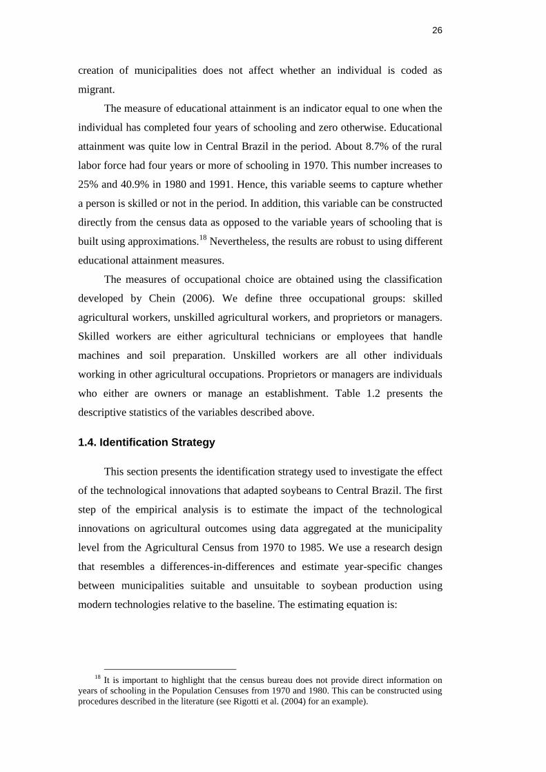
26

creation of municipalities does not affect whether an individual is coded as

migrant.

The measure of educational attainment is an indicator equal to one when the

individual has completed four years of schooling and zero otherwise. Educational

attainment was quite low in Central Brazil in the period. About 8.7% of the rural

labor force had four years or more of schooling in 1970. This number increases to

25% and 40.9% in 1980 and 1991. Hence, this variable seems to capture whether

a person is skilled or not in the period. In addition, this variable can be constructed

directly from the census data as opposed to the variable years of schooling that is

built using approximations.18

Nevertheless, the results are robust to using different

educational attainment measures.

The measures of occupational choice are obtained using the classification

developed by Chein (2006). We define three occupational groups: skilled

agricultural workers, unskilled agricultural workers, and proprietors or managers.

Skilled workers are either agricultural technicians or employees that handle

machines and soil preparation. Unskilled workers are all other individuals

working in other agricultural occupations. Proprietors or managers are individuals

who either are owners or manage an establishment. Table 1.2 presents the

descriptive statistics of the variables described above.

1.4. Identification Strategy

This section presents the identification strategy used to investigate the effect

of the technological innovations that adapted soybeans to Central Brazil. The first

step of the empirical analysis is to estimate the impact of the technological

innovations on agricultural outcomes using data aggregated at the municipality

level from the Agricultural Census from 1970 to 1985. We use a research design

that resembles a differences-in-differences and estimate year-specific changes

between municipalities suitable and unsuitable to soybean production using

modern technologies relative to the baseline. The estimating equation is:

18

It is important to highlight that the census bureau does not provide direct information on

years of schooling in the Population Censuses from 1970 and 1980. This can be constructed using

procedures described in the literature (see Rigotti et al. (2004) for an example).

27

𝑌𝑚𝑠𝑡 = 𝛼𝑚 + 𝛿𝑠𝑡 + ∑ 𝛾𝑣

1985

𝑣=1975

(𝑆𝑜𝑦𝑏𝑒𝑎𝑛 𝑃𝑜𝑡𝑒𝑛𝑡𝑖𝑎𝑙𝑚 ∗ 𝐼𝑣) + ∑ (𝑿𝑚 ∗ 𝐼𝑣)

1985

𝑣=1975

𝚪𝑣

+ 𝑢𝑚𝑠𝑡 (1.1)

where 𝑌𝑚𝑠𝑡 is an agricultural outcome in municipality 𝑚 in the state 𝑠 in the

period 𝑡; 𝛼𝑚 is a municipality fixed effect; 𝛿𝑠𝑡 is a state-time fixed effect;

𝑆𝑜𝑦𝑏𝑒𝑎𝑛 𝑃𝑜𝑡𝑒𝑛𝑡𝑖𝑎𝑙𝑚 is the agronomic potential to cultivate soybeans using

modern technologies; 𝐼𝑣 is a year indicator; 𝑿𝑚 is a vector of geographic and

initial characteristics; and 𝑢𝑚𝑠𝑡 is an error term. We cluster standard errors at the

municipality level in all specifications. The coefficients of interest are the three 𝛾𝑣

which represent the impact of the technological innovations in the different

sample periods. We allow the coefficients to change through time to differentiate

the impact of the technological innovations on agricultural outcomes during

different phases of the adaptation process.

The municipality fixed effects control for time invariant characteristics of

municipalities that might be correlated with soybean potential. The state-time

fixed effects controls for shocks specific to each of the four states included in the

sample. These shocks might either reflect different policies or different trends.19

Therefore, the identification assumption is that, within a state and in the absence

of the technological innovations, agricultural outcomes would have changed

similarly in municipalities with higher and lower potential to cultivate soybeans.

This is the equivalent of the parallel trends assumption from differences-in-

differences models. The difference is that it must hold within municipalities

located in each state and not across municipalities located in different states.

We include the controls 𝑿𝑚 to allow trends in agricultural outcomes differ

according to some observed municipal characteristics and relax the parallel trends

assumption. The controls can be divided in two groups. The first group

corresponds to geographic characteristics. The characteristics included are natural

logarithm of the distance to the coast and the distance to the federal capital. These

controls allow municipalities with different locations to benefit differentially from

the investments in infrastructure and in colonization made during the period. The

19

It is important to note that there were only two states in central Brazil in the beginning of

the period under analysis. Mato Grosso and Mato Grosso do Sul split in 1975 and Goiás and

Tocantins split in 1989. However, I include state-year fixed effects considering the four states that

exist in current days on the assumption that the important differences that exist across these states

were already relevant in the earlier period.

28

second group corresponds to baseline characteristics. The characteristics included

are the share of available land, log of the total farmland, log of the number of

farms, number of state-owned bank branches, number of private-owned bank

branches, and initial value of the dependent variable. These variables allow

municipalities with different characteristics to have different trends. Furthermore,

the inclusion of the initial value of the dependent variable as an additional control

controls for convergence in the outcomes.

The robustness exercises further test whether the parallel trends assumption

holds. We use data from the 1960 Agricultural Census to investigate whether

changes agricultural outcomes before the technological change were related to

soybean potential. The limit of the 1960 Agricultural Census data is that we do

not observe all outcomes observed in later periods and the robustness exercise can

be performed just for a subset of the outcomes used in the main estimates.

Another concern of the estimates is whether changes in international prices

are driving the results. We construct a price index combining data on crop output

in the baseline and soybean prices and show that the estimates are robust to its

inclusion. Other robustness exercises include controls for access to credit and land

tenure to mitigate concerns that changes in these variables that can be correlated

with soybean potential drive the estimates. These controls are not included in the

main estimates since the included variables are endogenous as technological

innovations can influence them. The main estimates are robust to the inclusion of

these additional covariates.

The second step of the empirical analysis is to estimate the impact of the

technological innovations on migration status and educational attainment using

individual level from the Population Census from 1970 to 1991. The empirical

design is the same used for agricultural outcomes with the difference that

outcomes are now observed at the individual level and that there are just three

sample periods. The estimating equation using individual data is:

𝑌𝑖𝑚𝑠𝑡 = 𝛼𝑚 + 𝛿𝑠𝑡 + ∑ 𝛾𝑣

1991

𝑣=1980

(𝑆𝑜𝑦𝑏𝑒𝑎𝑛 𝑃𝑜𝑡𝑒𝑛𝑡𝑖𝑎𝑙𝑚 ∗ 𝐼𝑣) + ∑ (𝑿𝑚 ∗ 𝐼𝑣)

1991

𝑣=1980

𝚪𝑣

+ 𝛽𝒁𝑖𝑚𝑠𝑡 + 𝑢𝑖𝑚𝑠𝑡 (1.2)

where 𝑌𝑖𝑚𝑠𝑡 is the outcome of interest from individual 𝑖 in municipality 𝑚,

state 𝑠 and period 𝑡 and 𝒁𝑖𝑚𝑠𝑡 is a vector of individual level controls. The

individual controls included are dummies for sex and for five-year age groups.

29

The other variables are the same variables included in equation (1.1). It is

not possible to include the initial value of the dependent variable as a control since

there is no panel data on individuals. Nevertheless, we do include the initial value

of the dependent variable in the municipality as a control.

The coefficients of interest are the 𝛾𝑣 estimated for 1980 and 1991. These

coefficients enable us to investigate the impact of technological innovations on

labor selection during different phases of the adaptation process. The

identification assumption needed for causal inference on these coefficients is the

same parallel trends assumption discussed above for the coefficients estimated in

equation (1.1). We cluster standard errors at the municipality-level in all

specifications estimated using equation (1.2).

1.5. Technological Change and Agricultural Modernization

1.5.1. Land Use

Table 1.3 presents the estimates of the impact of the technological

innovations on soybean adoption. The table aims to validate the measure of

agronomic potential and investigate whether municipalities more suitable for

soybean cultivation experienced faster increases in cultivation and production of

this crop. The table reports estimates of equation (1.1) for three different

outcomes: soybean cultivation per 1000 hectares, soybean production per 1000

hectares and the share of farms cultivating the crop.

Column 1 reports the effect of technological change on soybean cultivation

conditional on municipal and state-year fixed effects. Column 2 includes

geographic characteristics as controls while column 3 includes baseline

characteristics as controls. These columns provide evidence that municipalities

more suitable to soybean cultivation using modern technologies experienced

larger increases in soybean cultivation than municipalities less suitable for it in the

period 1970 to 1985. This finding validates the agronomic potential measure and

suggests that the comparative advantage to cultivate soybeans in Central Brazil

did not change after the sample period.

Columns 1 to 3 also show that the impact of the technological innovations

on soybean adoption grows over time. This result is consistent with the idea that

adaptation was a gradual process that allowed cultivation to occur in more areas.

30

It is also consistent with the idea that takes time for farmers to change agricultural

practices to adopt different crops and agricultural practices. The increases in the

coefficients suggest that the estimates are not capturing the impact of changes in

soybean prices, which increased at the beginning of the 1970s and decreased at

the end of this decade.

It is important to note that the addition of baseline controls reduces the size

of the estimated impact of the technological innovations. That suggests that the

inclusion of baseline characteristics is essential for the empirical design. The

magnitude of the estimated impact of the technological innovations is substantial.

One standard deviation increase in agronomic potential is associated with a

relative increase in 14.2 to 17.5 hectares in soybean cultivation per thousand

hectares of farmland from 1970 to 1985. The results provide evidence that the

agronomic potential measure is a useful indicator of the gain that technological

innovations brought to farmers in Central Brazil.

Columns 4 to 6 report the effects of technological innovations on soybean

production using the same specifications used in columns 1 to 3. The results are

similar to the ones discussed above. Production increased faster in municipalities

more suitable to soybean cultivation. The estimated increases are larger in later

periods and are reduced with the inclusion of controls. The magnitude of the

estimated impact is also substantial. One standard deviation increase in agronomic

potential is associated with a relative increase in 24.6 to 34.5 tons in soybean

production per thousand hectares of farmland from 1970 to 1985. A back of the

envelope calculation comparing estimates in columns 1-3 with estimates in

columns 4-6 from the same table suggest that the technological innovations

increased yields by about 80%.

Columns 7 to 9 report the effect of the technological innovations on the

share of farms cultivating the crop. The results point out that the technological

change had a significant impact on the share of farms producing the crop both in

1980 and 1985. The effects estimated in 1975 are not significant across

specifications (despite the point estimates being positive in all columns). This

result suggests that expansion of crop cultivation was not restricted to the

intensive margin.

An important question is whether the technological innovations affected

land use in general. To answer this question, Table 1.4 reports estimates of the

31

impact of technological change on land use. The table reports estimates equation

(1.1) for three different outcomes: the share of cropland, the share of pastures and

the share of forests. Columns 1, 4 and 7 report the estimates obtained conditional

on municipal and state-year fixed effects. Columns 2, 5 and 8 report the estimates

obtained conditional also on geographic characteristics. Columns 3, 6 and 9 report

the estimates obtained conditional also on baseline agricultural characteristics.

In columns 1 to 3 we find that the technological innovations increased the

share of cropland both in 1980 and 1985. The effects are significant in all three

specifications. Their magnitudes suggest that one standard deviation increase in

agronomic potential is associated with a rise in 1.3 to 2.2 percentage points in the

share of cropland from 1970 to 1980 and 1.9 to 2.7 percentage points in this

variable from 1970 to 1985. These magnitudes are substantial since cropland

represented just 6% of the total farmland in the baseline. This result evidences that

soybean cultivation did not expand replacing other crops. Indeed, the total

estimated increase cropland is even larger than the estimated increased in soybean

cultivation, which is consistent with the idea that the technological innovations

had positive spillovers to the production of other crops.20

The evidence from the remaining columns suggests that cropland expanded

over pastures (columns 4 to 6) and not over forests (columns 7 to 9). On the one

hand, the share of pastures declines in more suitable municipalities in all

specifications. The relative decline in pastures from 1970 to 1985 is significant at

the 10% level in column 4, at the 5% level in column 5, and not significant in

column 6. On the other hand, the changes in forests have no clear pattern. The

coefficients switch from being positive to negative across different periods and

specifications. These findings suggest that technological innovations inducing

farmers to invest in agricultural intensification rather than in land clearing.

1.5.2. Input Use

The results from Tables 1.3 and 1.4 provide evidence that soybean

adaptation shifted land use from pasture to crop cultivation. We argued before that

crop cultivation requires agricultural practices quite different from the ones used

20

There are several reasons that indicate that such spillovers exist. Investments in machines

might enable production of other crops in areas not suited to soybean cultivation. Moreover, there

might be agronomic benefits from rotating land across different crops.

32

in cattle grazing. Therefore, it is expected that the technological innovations

affected the use of inputs.

Table 1.5 presents evidence consistent with this idea. It reports estimates of

the impact of technological change obtained using equation (1.1) on labor use,

tractor use and liming use. We choose liming as the measure of fertilizer use since

it is recognized to be the main fertilizers needed to cultivate crops in Cerrado

lands (Spehar, 1996; Rezende, 2002). Estimates from columns 1 to 3 report the

results for labor use, estimates from columns 4 to 6 report the results for tractor

use and estimates from columns 7 to 9 report the results for liming use. The

specifications are the same used before.

Columns 1 to 3 point out that the technological innovations had no effect on

the total labor use in agriculture. In the period 1970 to 1985, total labor use

increased at similar rates in municipalities more and less suitable for soybean

cultivation using modern technologies. More productive agriculture neither

increased total labor force in agriculture as in Foster and Rosenzweig (2008) and

Hornbeck and Keskin (Forthcoming) nor decreased it as in Bustos et al. (2014).

The remaining columns present evidence that technological innovations

increased the use or modern inputs in agriculture. Columns 4 to 6 show that the

technological innovations induced farmers to adopt machines. Following the

technological innovations, the number of tractors increased faster in

municipalities more suitable for soybean cultivation. The effects are significant in

all specifications and indicate that one standard deviation increase in the potential

measure led to a growth in .33 to .41 in the number of tractors per thousand

hectares from 1970 to 1985. Columns 7 to 9 report that the technological

innovations also induced farmers to adopt fertilizers. The effects are also

significant in all three specifications and suggest that one standard deviation

increase in agronomic potential is associated with a rise in 1.9 to 2.9 percentage

points in the share of farms using liming from 1970 to 1985. These impacts are

consistent with the idea that crop cultivation in Central Brazil required

mechanization and fertilizers to be feasible.

It is important to notice that the effect of the technological innovations on

liming use decline from 1980 to 1985. This result is inconsistent with previous

findings that indicate that the impacts of the innovations increase over time. The

33

expansion of the use of this fertilizer on pastures might explain this result.21

Data

on the total expenditure on fertilizers and pesticides suggests that this might be the

case. We find that the effects of technological innovations on these expenditures

are positive and increase over time (these estimates are available upon request).

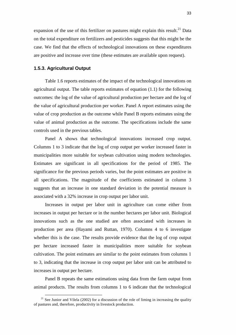
1.5.3. Agricultural Output

Table 1.6 reports estimates of the impact of the technological innovations on

agricultural output. The table reports estimates of equation (1.1) for the following

outcomes: the log of the value of agricultural production per hectare and the log of

the value of agricultural production per worker. Panel A report estimates using the

value of crop production as the outcome while Panel B reports estimates using the

value of animal production as the outcome. The specifications include the same

controls used in the previous tables.

Panel A shows that technological innovations increased crop output.

Columns 1 to 3 indicate that the log of crop output per worker increased faster in

municipalities more suitable for soybean cultivation using modern technologies.

Estimates are significant in all specifications for the period of 1985. The

significance for the previous periods varies, but the point estimates are positive in

all specifications. The magnitude of the coefficients estimated in column 3

suggests that an increase in one standard deviation in the potential measure is

associated with a 32% increase in crop output per labor unit.

Increases in output per labor unit in agriculture can come either from

increases in output per hectare or in the number hectares per labor unit. Biological

innovations such as the one studied are often associated with increases in

production per area (Hayami and Ruttan, 1970). Columns 4 to 6 investigate

whether this is the case. The results provide evidence that the log of crop output

per hectare increased faster in municipalities more suitable for soybean

cultivation. The point estimates are similar to the point estimates from columns 1

to 3, indicating that the increase in crop output per labor unit can be attributed to

increases in output per hectare.

Panel B repeats the same estimations using data from the farm output from

animal products. The results from columns 1 to 6 indicate that the technological

21

See Junior and Vilela (2002) for a discussion of the role of liming in increasing the quality

of pastures and, therefore, productivity in livestock production.

34

change did not affect the log of the value of animal production neither per labor

unit nor area. These findings point out that the reduction in pastures did not

decrease output from animal products. Either the marginal product of the land

converted from pasture to crops was close to zero or that spillovers from better

agricultural practices offset the reduction in pastures.

These results reinforce the interpretation that the estimates capture the

impact of the technological innovations in crop cultivation (as opposed to general

improvements in agricultural practices). In addition, these suggest that general

equilibrium considerations arising from the displacement of cattle grazing from

areas that benefited from the technological innovations to areas that did not

benefit from it do not seem to be relevant.

1.6. Technological Change and Labor Selection

1.6.1. Migration Status

Table 1.7 reports estimates of the impact of the technological innovations on

migration status. It reports estimates of equation (1.2) in which the outcome of

interest is an indicator equal to one if the individual is a migrant. Estimates

consider the full sample described in the data section. Columns 1 to 3 define

migrants as individuals not born in the state. Columns 4 to 6 define migrants as

individuals not born in the municipality.

In columns 1 to 3 we estimate that the share of migrants in the labor force

increased faster in municipalities more suitable for soybean cultivation. The

estimates are not significant at the usual statistical levels in column 1 but are

significant in columns 2 and 3. The impact of the technological innovations

increases over time with the coefficients estimated in 1991 being larger than the

coefficients estimated in 1980. The magnitude of the impact of the technological

innovations is substantial: an increase in one standard deviation in agronomic

potential is associated with an increase in 1.9 percentage points in the likelihood

that an individual was not born in the state from 1970 to 1980 and an increase in

3.6 percentage points from 1970 to 1991.

It should be noted that the definition of migration used in the estimates from

columns 1 to 3 is a conservative measure of migration. It underestimates total

migration as it does not consider individuals who migrate within a state. We use

35

this variable as the preferred migration measure because it is less affected by

measurement error. Columns 4 to 6 provide evidence that the results are robust to

using an alternative migration definition. Technological innovations increase the

migration rate in all specifications and point estimates are even larger than the

ones obtained using the preferred migration measure.

These results provide evidence that migration increased in response to the

technological innovations. Since the total labor force remained constant, the rise

in the share of migrants indicates that both immigration and emigration increased.

More individuals sort into and out of the rural sector in municipalities which

benefit from the technological innovations.

1.6.2. Educational Attainment

One interpretation for the increase in migration rates documented in the

previous subsection is that population movements are responding to changes in

the demand for human capital in agriculture. This interpretation suggests that

technological innovations should affect the educational attainment of the rural

labor force. Table 1.8 investigates whether this is the case. It reports estimates of

the impact of technological innovations on schooling using equation (1.2). The

outcome of interest is an indicator equal to one if the individual completed four

years of more of formal schooling. Columns 1 to 3 report estimates for the full

sample. Columns 4 to 6 report estimates for a subsample of individuals born in the

state (natives). Columns 7 to 9 report estimates for a subsample of individuals

born in another state (migrants).

Columns 1 to 3 point out that educational attainment increased faster in

municipalities more suitable for soybean cultivation. The effects of the

innovations are significant at the usual statistical levels across all specifications.

These impacts increases over time with the coefficients estimated for 1991 being

twice the size of the coefficients estimated for 1980. The magnitudes of these

coefficients suggest that an increase in one standard deviation in agronomic

potential is associated with an increase in 1.9 percentage points in the likelihood

that an individual has four or more years of schooling from 1970 to 1980 and an

increase in 3.3 percentage points in this likelihood from 1970 to 1991. These

effects are large since just 8.7% of the agricultural labor force had four years or

more of schooling in the baseline.

36

The results described above are consistent with technological innovations

affecting either selective migration or investments in skill acquisition. We divide

the sample between individuals who were born in the state (natives) and

individuals who were born in another state (migrants) to separate these channels.

An increase in educational attainment among natives can reflect both selection

and skill acquisition. Nevertheless, an increase in educational attainment among

migrants reflects selection.22

Columns 4 to 6 present estimates for the sample of

natives while columns 7 to 9 present estimates for the sample of migrants.

The results point out that technological change increased educational

attainment both among natives and migrants. The estimated impacts are

significant in all specifications in the natives subsample (columns 4 to 6) and the

specifications including controls in the migrants subsample (columns 8 and 9).

The estimates in the more saturated specifications in columns 6 and 9 from Table

1.8 are larger in magnitude in the subsample of migrants. The results on migrants

provide evidence that labor selection helps to drive the rise in educational

attainment.

To assess the importance of the selection mechanism, we can perform a

calculation assuming that selection accounts for all the increase in educational

attainment among migrants while skill acquisition accounts for all the increase

among natives. Given the size of the migrant cohort, our estimates suggest that

about half of the increase in educational attainment can be attributed to labor

selection.

Table 1.9 reports estimates of the impact of technological change on

educational attainment for cohorts born from 1930 to 1955. These cohorts were at

least 15 years old in 1970, which implies that the technological innovations did

not affect their schooling choices during school age. While individuals can return

to school later, this is rare and the effects of the technological innovations on

educational attainment among these cohorts are expected to reflect selection rather

than skill acquisition. Columns 1 to 9 report estimates including the same controls

included in columns 1 to 9 from Table 1.8.

The results from Table 1.9 are similar to the ones from the previous table.

These findings provide evidence that selection can be even more important to

22

We are assuming that there are no general equilibrium impacts of the technological change

that increase the return to skill in all locations.

37

explain the rise in educational attainment than the calculation performed above

suggested. However, it is important to note that the magnitude of the estimates is

smaller in most specifications. That is suggestive that skill acquisition explains at

least some of the increase in educational attainment documented in Table 1.8.

Older individuals are thought to have more specific human capital and

higher moving costs than younger ones. This fact suggests that the effects of

technological innovations on the composition of the labor force might be more

intense among some cohorts. We estimate cohort-specific impacts of the

technological innovations to investigate whether their effect is heterogeneous

across cohorts. Estimates include individuals born from 1930 to 1955 and are

obtained estimating the following equation:

𝑌𝑖𝑚𝑠𝑡 = 𝛼𝑚 + 𝛿𝑠𝑡 + ∑ ∑ 𝛾𝑣𝑐

1955

𝑐=1930

1991

𝑣=1980

(𝑆𝑜𝑦𝑏𝑒𝑎𝑛 𝑃𝑜𝑡𝑒𝑛𝑡𝑖𝑎𝑙𝑚 ∗ 𝐼𝑣 ∗ 𝐼𝑐)

+ ∑ 𝛉𝑣

1991

𝑣=1980

(𝑿𝑚 ∗ 𝐼𝑣) + 𝛽𝒁𝑖𝑚𝑠𝑡 + 𝑢𝑖𝑚𝑠𝑡 (1.3)

where 𝐼𝑐 is an indicator that takes value one when the individual belongs to

cohort 𝑐. The parameters 𝛾𝑣𝑐 estimate whether educational attainment of each

cohort increased faster in municipalities with higher agronomic potential

compared to municipalities with lower agronomic potential during the period

1970 to 1991. The identification assumption on these parameters is that

educational attainment of each cohort would have evolved in a similar fashion in

municipalities with different levels of agronomic potential in the absence of the

technological innovations that adapted soybean to Central Brazil.

Figure 1.2 reports the results. It plots the cohort-specific effects of the

technological innovations on educational attainment. Panel A presents the

estimates of 𝛾1980𝑐 for different cohorts of natives. Panel B presents the estimates

of 𝛾1991𝑐 for different cohorts of natives. Panel C presents the estimates of 𝛾1980𝑐

for different cohorts of migrants. Panel D presents the estimates of 𝛾1991𝑐 for

different cohorts of migrants. The reported estimates included state-year fixed

effects, cohort fixed effects, sex dummies and geographic and baseline

characteristics as controls.

The estimates plotted in all four panels indicate that the increases in

educational attainment are concentrated among younger cohorts. In the natives

38

subsample, the effect of technological innovations on educational attainment is

concentrated among cohorts born after 1950 in the first treatment period (Panel A)

and after 1945 in the second treatment period (Panel B). In the migrants

subsample, these effects are concentrated among cohorts born after 1940 in the

first treatment period (Panel C) and after 1945 in the second treatment period

(Panel D). The comparison of the cohort-specific impact of the technological

change on educational attainment among migrants (Panels C and D) and natives

(Panels A and B) reveals that the effect in the former group is higher than in the

latter. There are also more cohorts of migrants which are affected than there are

cohorts of natives.

Overall the results from this subsection suggest that technological

innovations induced immigration of skilled individuals to municipalities that

benefited more from it. The findings also suggest that the innovations induced

emigration of unskilled individuals from these municipalities. Both movements

are concentrated among cohorts facing lower migration costs and result in an

increase in the overall educational attainment of the rural labor force.

1.6.3.Occupational Choices

Table 1.10 reports estimates of the impact of technological change on

occupational choices. It reports estimates of equation (1.2) for the following

outcomes of interest: an indicator equal to one if the individual works in a skilled

occupation in agriculture; an indicator equal to one if the individual works in an

unskilled occupation in agriculture and; an indicator equal to one in the individual

is either a manager or a proprietor. Columns 1 to 3 report estimates in which the

outcome is whether the individual works in a skilled occupation in agriculture.

Columns 4 to 6 report estimates in which the outcome is whether the individual

works in an unskilled occupation in agriculture. Columns 7 to 9 in which the

outcome is whether the individual is a manager or a proprietor.

Columns 1 to 3 point out that the share of labor working in skilled

agricultural occupations increased faster in municipalities more suitable for

soybean cultivation. The estimated impacts are significant and robust across

specifications. This finding suggests that the technological innovations might have

affected migration and the composition of the rural labor force through changes in

the jobs available in the sector. Crop cultivation and the adoption of modern

39

agricultural practices created employment opportunities for individuals with

higher-than-average human capital and induced their migration to municipalities

in which crop cultivation and agricultural intensification were happening.

The impact of the technological change increases over time with the

coefficients estimated in 1991 being about 2.2 times the coefficients estimated in

1980. The estimated magnitudes suggest that an increase in one standard deviation

in soybean potential is associated with an increase in .5 percentage points in the

likelihood that an individual works in a skilled occupation from 1970 to 1980 and

an increase in 1.2 percentage points in the same measure from 1970 to in 1991.

Columns 4 to 6 indicate that the share of labor working in unskilled

agricultural occupations declined faster in municipalities more suitable for

soybean cultivation. This result provides evidence that the technological change

induced farms to replace unskilled labor for skilled labor. Fewer job opportunities

for individuals with lower-than-average human capital stimulated their emigration

from municipalities that benefited from the technological innovations. Columns 7

to 9 provide evidence that the share of the labor force working as managers or

proprietors did not increase faster in more suitable municipalities. That suggests

that the technological change did not induce changes in the use of managerial

capital in agriculture.

1.6.4. Selection and Agricultural Output

Table 1.11 re-estimates the impact of the technological innovations on

agricultural output including aggregate measures of schooling and occupational

choices as controls. These estimations aim to provide tentative evidence on the

quantitative importance of the selection pattern documented above on aggregate

output. It is expected that the inclusion of these controls will reduce the impact of

the technological change on agricultural output whenever labor selection is

important to drive the increase in agricultural production.

We first re-estimate the specification from columns 3 and 6 from Table 1.6

using data either for 1970 and 1980 or 1970 and 1985. The results from these

specifications are presented in columns 1, 3, 5 and 7 from Table 1.11. We then

include the average educational attainment and the share of the agricultural labor

force in skilled occupations as controls in columns 2, 4, 6 and 8. Columns 2 and 4

uses data from the Population Census from 1980 to construct these measures

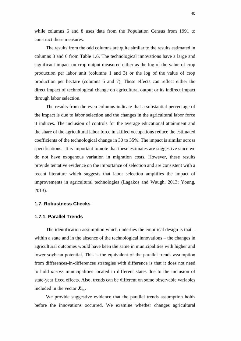
40

while columns 6 and 8 uses data from the Population Census from 1991 to

construct these measures.

The results from the odd columns are quite similar to the results estimated in

columns 3 and 6 from Table 1.6. The technological innovations have a large and

significant impact on crop output measured either as the log of the value of crop

production per labor unit (columns 1 and 3) or the log of the value of crop

production per hectare (columns 5 and 7). These effects can reflect either the

direct impact of technological change on agricultural output or its indirect impact

through labor selection.

The results from the even columns indicate that a substantial percentage of

the impact is due to labor selection and the changes in the agricultural labor force

it induces. The inclusion of controls for the average educational attainment and

the share of the agricultural labor force in skilled occupations reduce the estimated

coefficients of the technological change in 30 to 35%. The impact is similar across

specifications. It is important to note that these estimates are suggestive since we

do not have exogenous variation in migration costs. However, these results

provide tentative evidence on the importance of selection and are consistent with a

recent literature which suggests that labor selection amplifies the impact of

improvements in agricultural technologies (Lagakos and Waugh, 2013; Young,

2013).

1.7. Robustness Checks

1.7.1. Parallel Trends

The identification assumption which underlies the empirical design is that –

within a state and in the absence of the technological innovations – the changes in

agricultural outcomes would have been the same in municipalities with higher and

lower soybean potential. This is the equivalent of the parallel trends assumption

from differences-in-differences strategies with difference is that it does not need

to hold across municipalities located in different states due to the inclusion of

state-year fixed effects. Also, trends can be different on some observable variables

included in the vector 𝑿𝑚.

We provide suggestive evidence that the parallel trends assumption holds

before the innovations occurred. We examine whether changes agricultural

41

outcomes before the technological innovations were related to agronomic

potential using these modern technologies. This provides evidence that trends

were similar before the technological innovations.

A limitation of this robustness test is that we lack data before 1970 for

several outcomes. Therefore, the exercise is performed only for some outcomes

presented in the previous estimates. To implement the robustness test we also

have to account for the creation of municipalities and border changes in the period

1960 to 1970. The total sample has 193 municipalities. The results are presented

in Table 1.12 and indicate that changes in agricultural outcomes were similar

across municipalities with different agronomic potential before the innovations

occurred. We report estimates including geographic controls. Results available

upon request provide evidence that the results are similar either excluding

geographic controls or including initial characteristics.

1.7.2. Agricultural Prices

One important concern is that changes in agricultural prices drive the

estimates. Some accounts suggest that the expansion of soybean cultivation during

the 1970s was led by increases in soybean prices (Kiihl and Calvo, 2008). Indeed,

the data from the agricultural censuses indicates that prices received by farmers

rose between 1970 and 1975 as fish flour production in Peru collapsed.23

Prices

fell from 1975 to 1980 and remain stable afterwards.

The pattern of the coefficients suggests that changes in prices do not seem to

drive the results. Impacts are much higher in later periods when prices were

falling. We provide further evidence that prices are not driving the results

including a control for soybean prices in the estimates. The control is denominated

is the product of value of crop production as a share of total agricultural

production in the baseline period and the average farm gate soybean price in the

municipalities in the sample. The intuition of this variable is that municipalities in

which crop production is more important benefit more from increases in soybean

prices.

The results from estimates including this variable as a control are presented

in Tables 1.13 and 1.14. Columns 1 to 3 from Table 1.13 present the results for

23

Fish flour is another important source of animal protein.

42

agricultural outcomes while columns 1 and 2 from Table 1.14 present estimates

for socioeconomic outcomes. In this and in the following robustness tests, we

focus in three agricultural outcomes (share of crops, tractor use and crop output)

and two socioeconomic outcomes (educational attainment and occupational

choice). The results from both tables indicate that prices increases do not drive the

estimates presented in the previous sections.

1.7.3. Land Tenure

Another concern is that colonization projects induced changes in land tenure

that drive the main results. Public and private colonization projects are a

characteristic of the expansion of the Brazilian agricultural frontier in the period

(Alston et al., 1996; Jepson, 2002). To the extent that these colonization projects

and the changes in land tenure associated with them are correlated with the

agronomic potential measure, the results might confound the impact of the

technological innovations and the impact of land tenure. This might be relevant

since the literature indicates that land tenure is an important determinant of

investments among farmers (Banerjee et al., 2002; Goldstein and Udry, 2008).

We include the share of the farmland cultivated by tenants and by

occupants to examine whether the main results are driven by the expansion of

bank branches. It is important to note that these controls are endogenous as

technological change can affect the demand for land titling. However, including

these controls in the estimates is useful to examine the robustness of the main

results. The results from these estimates are presented in Tables 1.13 and 1.14.

Columns 4 to 6 from Table 1.13 present the results for agricultural outcomes

while columns 3 and 4 from Table 1.14 present estimates for socioeconomic

outcomes. The results from both tables indicate that the estimates are robust to

changes in land tenure that happened in the period.

1.7.4. Access to Credit

A final concern is that the expansion in agricultural credit drives the main

results. A large expansion in the number of bank branches in the period (Graham

et al., 1987). The existing literature suggests that changes in the number of bank

43

branches can be important to agricultural development in environments in which

credit constraints are pervasive (Burgess and Pande, 2005).

The expansion in bank branches could affect more municipalities more

suitable for soybean cultivation using modern technologies under the assumption

that credit constraints are more important constraints to the expansion of crop

agriculture than to other agricultural activities. Therefore, the main results might

confound the impact of the technological change with the impact of the expansion

in the number of bank branches.

We control for the number of bank branches (both private and state-owned)

to examine whether the main results are sensitive to the addition of these

covariates. These controls are endogenous as technological innovations can affect

total credit demand and – through this channel – the number of bank branches.

Nevertheless, the estimates are important to examine the robustness of the main

results. The results from these estimates are presented in Tables 1.13 and 1.14.

Columns 7 to 9 from Table 1.13 present the results for agricultural outcomes

while columns 5 and 6 from Table 1.14 present estimates for socioeconomic

outcomes. The results from both tables indicate that the estimates are robust to

changes in the number of bank branches that happened in the period.

1.8. Conclusion

In this paper, we use detailed data on agricultural potential to estimate the

causal impact of technological innovations that adapted soybeans for Central

Brazil. We estimate that these innovations induced farmers to convert pasture into

crops and to adopt modern inputs such as tractors and fertilizers. We also estimate

that innovations led to selection of unskilled labor out of agriculture and selection

of skilled labor into this sector.

These results illustrate the connection between technological innovations

and the composition of the rural labor force and complement earlier empirical

evidence on the connection of technological innovations and the size of the rural

labor force (Caselli and Coleman II, 2001; Foster and Rosenzweig, 2008; Nunn

and Qian, 2011; Bustos et al., 2014; Hornbeck and Keskin, Forthcoming). This

historical episode suggests that changes in production possibilities in agriculture

have different impacts across the various groups of workers. This finding can have

44

significant implications for the debate on agricultural policies and adjustment to

climatic change.

This episode also provides evidence that complementarities between human

capital and modern agricultural technologies induce substantial changes in the

composition of the rural labor force in response to technological innovations.

These responses are similar to the ones predicted by the models presented in

Lagakos and Waugh (2013) and Young (2013). Hence, we provide evidence that

the labor selection mechanism emphasized in these papers has empirical relevance

and might account for the observed differentials in income between agricultural

and non-agricultural activities.

45

Figure 1.1 – Soybean Potential in Central Brazil

Notes: Data source is FAO-GAEZ. Soybean potential is the difference in potential soybean yields under the high and the low input regime.

46

Figure 1.2 – Technological Change and Educational Attainment across Cohorts

Notes: The solid lines report the effect of the technological change on educational attainment across cohorts. Estimates are obtained estimating equation (1.3) in the main text for subsamples of

migrants and natives. Sample includes individuals born from 1930 to 1955 either employed or looking for a job living in municipalities in the states of Goiás, Mato Grosso, Mato Grosso do Sul

and Tocantins. Controls used are age of birth, sex, state-year fixed effects and geographic and baseline characteristics interacted with time dummies. Dashed lines represent 95% confidence

intervals obtained estimating standard errors clustered at the municipality level.

-.05

0

.05

.1

193

1

193

2

193

3

193

4

193

5

193

6

193

7

193

8

193

9

194

0

194

1

194

2

194

3

194

4

194

5

194

6

194

7

194

8

194

9

195

0

195

1

195

2

195

3

195

4

195

5

193

1

193

2

193

3

193

4

193

5

193

6

193

7

193

8

193

9

194

0

194

1

194

2

194

3

194

4

194

5

194

6

194

7

194

8

194

9

195

0

195

1

195

2

195

3

195

4

195

5

Panel A: Natives (1980) Panel C: Migrants (1980)

-.05

0

.05

.1.1

5

193

1

193

2

193

3

193

4

193

5

193

6

193

7

193

8

193

9

194

0

194

1

194

2

194

3

194

4

194

5

194

6

194

7

194

8

194

9

195

0

195

1

195

2

195

3

195

4

195

5

193

1

193

2

193

3

193

4

193

5

193

6

193

7

193

8

193

9

194

0

194

1

194

2

194

3

194

4

194

5

194

6

194

7

194

8

194

9

195

0

195

1

195

2

195

3

195

4

195

5

Panel B: Natives (1991) Panel D: Migrants (1991)

47

Table 1.1: Descriptive Statistics – Agricultural Censuses

1970 1975 1980 1985

Panel A: Soybeans

Cultivation per 1000 hectares 0.415 (0.105) 2.282 (0.618) 7.688 (1.842) 15.686 (2.575)

Production per 1000 hectares 0.362 (0.099) 3.243 (0.956) 13.587 (3.411) 29.655 (5.024)

Share of Farms 0.714 (0.228) 1.299 (0.394) 2.065 (0.467) 3.272 (0.527)

Panel B: Land Use

Share of Cropland 6.077 (0.455) 7.626 (0.515) 8.163 (0.476) 8.755 (0.510)

Share of Pasture 67.525 (1.068) 68.579 (0.998) 67.428 (0.865) 69.192 (0.769)

Share of Forests 14.046 (0.829) 13.435 (0.873) 13.027 (0.733) 11.478 (0.586)

Panel C: Input Use

Labor Use 21.842 (1.333) 23.105 (1.292) 22.805 (1.220) 24.652 (1.289)

Tractor Use 0.246 (0.025) 0.498 (0.044) 0.848 (0.053) 1.083 (0.065)

Liming Use 0.319 (0.047) 0.844 (0.099) 3.809 (0.355) 4.601 (0.365)

Panel D: Agricultural Output

Log of Crop Output per Labor Unit 3.568 (0.073) 4.060 (0.072) 4.288 (0.071) 4.395 (0.074)

Log of Crop Output per Hectare 7.755 (0.039) 8.155 (0.049) 8.377 (0.053) 8.401 (0.059)

Notes: All variables are observed for the 254 municipalities in the sample. Standard deviations are reported in parentheses.

48

Table 1.2: Descriptive Statistics - Population Censuses

1970 1980 1991

Panel A: Migration

Not Born in the State 0.459 (0.001) 0.445 (0.001) 0.392 (0.001)

Not Born in the Municipality 0.596 (0.001) 0.633 (0.001) 0.590 (0.002)

Panel B: Educational Attainment

Four Years or More of Schooling (0/1) - Full Sample 0.087 (0.001) 0.250 (0.001) 0.409 (0.002)

Four Years or More of Schooling (0/1) - Natives 0.089 (0.001) 0.253 (0.001) 0.410 (0.002)

Four Years or More of Schooling (0/1) - Migrants 0.085 (0.001) 0.246 (0.002) 0.409 (0.002)

Panel C: Occupational Choices

Skilled Occupation (0/1) 0.006 (0.000) 0.037 (0.000) 0.040 (0.001)

Unskilled Occupation (0/1) 0.006 (0.000) 0.037 (0.000) 0.040 (0.001)

Proprietor or Manager (0/1) 0.030 (0.000) 0.057 (0.001) 0.065 (0.001)

Notes: All variables are observed for the 254 municipalities in the sample. Standard deviations are reported in parentheses.

49

Table 1.3: The Effect of Technological Change on Soybean Adoption

Cultivation Production Share of Farms

(1) (2) (3) (4) (5) (6) (7) (8) (9)

Soybean Potential x 1975 5.609*** 5.075*** 2.731** 8.630*** 7.868*** 2.945** 1.287** 1.015** 0.458

(1.945) (1.816) (1.104) (3.016) (2.841) (1.331) (0.504) (0.500) (0.340)

Soybean Potential x 1980 18.645*** 17.671*** 11.618*** 34.842*** 32.857*** 17.793*** 3.706*** 3.824*** 3.202***

(5.539) (5.333) (3.947) (10.350) (9.947) (6.457) (1.083) (1.096) (1.094)

Soybean Potential x 1985 29.987*** 29.561*** 24.314*** 59.249*** 57.658*** 42.118*** 5.290*** 5.571*** 4.925***

(6.704) (6.660) (5.527) (12.998) (12.843) (9.825) (1.268) (1.288) (1.304)

Municipality FE Yes Yes Yes Yes Yes Yes Yes Yes Yes

State x Year FE Yes Yes Yes Yes Yes Yes Yes Yes Yes

Geographic Controls x Year No Yes Yes No Yes Yes No Yes Yes

Baseline Controls x Year No No Yes No No Yes No No Yes

Observations 1,016 1,016 1,016 1,016 1,016 1,016 1,016 1,016 1,016

Number of Municipalities 254 254 254 254 254 254 254 254 254

Notes: The table reports estimates from equation (1.1) in the text. The dependent variables are reported on the top of the respective columns. Cultivation is the number of hectares cultivated with

soybeans by each thousand hectares of farmland. Production is the soybean production by each thousand hectares of farmland. Share of Farms is the share of farms which cultivates soybeans.

Soybean Potential is the difference of the potential soybean yields under high inputs and under low inputs. Geographic Controls x Year are the interaction between year dummies and the log of

the distance to Brasília and the log of the distance to the coast. Baseline Controls x Year are the interaction between year dummies are the baseline value of the share of available land, the log of

the number of farms, the log of total farmland, the number of state-owned bank branches, the number of private bank branches and the dependent variable. The sample is composed by all

municipalities in the states of Mato Grosso do Sul, Mato Grosso, Goiás and Tocantins for the years 1970, 1975, 1980 and 1985. Standard errors clustered at the municipality level are reported in

parentheses. * denotes statistical significance at 10% ** denotes statistical significance at 5% *** denotes statistical significance at 1%.

50

Table 1.4 The Effect of Technological Change on Land Use

Share of Cropland Share of Pasture Share of Forest

(1) (2) (3) (4) (5) (6) (7) (8) (9)

Soybean Potential x 1975 1.292 1.691** 1.791* -0.884 -1.891 0.859 -0.468 -0.420 -2.365

(0.835) (0.851) (0.941) (1.329) (1.519) (1.720) (1.472) (1.685) (1.700)

Soybean Potential x 1980 2.317*** 2.700*** 3.988*** -1.711 -3.925** -0.096 1.271 2.908 0.360

(0.861) (0.852) (0.961) (1.732) (1.753) (1.901) (1.547) (2.312) (1.843)

Soybean Potential x 1985 3.289*** 4.015*** 5.227*** -3.967* -7.683*** -2.126 0.847 3.003 -0.342

(0.857) (0.850) (1.072) (2.212) (2.199) (2.007) (1.513) (1.969) (1.329)

Municipality FE Yes Yes Yes Yes Yes Yes Yes Yes Yes

State x Year FE Yes Yes Yes Yes Yes Yes Yes Yes Yes

Geographic Controls x Year No Yes Yes No Yes Yes No Yes Yes

Baseline Controls x Year No No Yes No No Yes No No Yes

Observations 1,016 1,016 1,016 1,016 1,016 1,016 1,016 1,016 1,016

Number of Municipalities 254 254 254 254 254 254 254 254 254

Notes: The table reports estimates from equation (1.1) in the text. The dependent variables are reported on the top of the respective columns. Share of Cropland is the share of farmland

cultivated with temporary crops. Share of Pasture is the share of farmland covered with pasture. Share of Forests is the share of farmland covered with forests. Soybean Potential is the

difference of the potential soybean yields under high inputs and under low inputs. Geographic Controls x Year are the interaction between year dummies and the distance to Brasília and the

distance to the coast. Baseline Controls x Year are the interaction between year dummies are the baseline value of the share of available land, the log of the number of farms, the log of total

farmland, the number of state-owned bank branches, the number of private bank branches and the dependent variable. The sample is composed by all municipalities in the states of Mato Grosso

do Sul, Mato Grosso, Goiás and Tocantins for the years 1970, 1975, 1980 and 1985. Standard errors clustered at the municipality level are reported in parentheses. * denotes statistical

significance at 10% ** denotes statistical significance at 5% *** denotes statistical significance at 1%.

51

Table 1.5: The Effect of Technological Change on Input Use

Labor Use Tractor Use Liming Use

(1) (2) (3) (4) (5) (6) (7) (8) (9)

Soybean Potential x 1975 -0.120 2.305 -2.431 0.241*** 0.248*** 0.160** 0.891*** 0.747** 0.657***

(1.824) (3.217) (1.841) (0.089) (0.095) (0.078) (0.320) (0.291) (0.214)

Soybean Potential x 1980 0.648 3.566 -0.600 0.395*** 0.436*** 0.366*** 5.430*** 5.304*** 3.821***

(1.924) (3.503) (2.009) (0.091) (0.092) (0.100) (1.011) (0.995) (0.870)

Soybean Potential x 1985 0.801 4.493 1.201 0.618*** 0.697*** 0.562*** 4.983*** 4.899*** 3.261***

(1.913) (3.191) (1.927) (0.122) (0.127) (0.130) (0.969) (0.959) (0.831)

Municipality FE Yes Yes Yes Yes Yes Yes Yes Yes Yes

State x Year FE Yes Yes Yes Yes Yes Yes Yes Yes Yes

Geographic Controls x Year No Yes Yes No Yes Yes No Yes Yes

Baseline Controls x Year No No Yes No No Yes No No Yes

Observations 1,016 1,016 1,016 1,016 1,016 1,016 1,016 1,016 1,016

Number of Municipalities 254 254 254 254 254 254 254 254 254

Notes: The table reports estimates from equation (1.1) in the text. The dependent variables are reported on the top of the respective columns. Labor Use is total employment per thousand

hectares of farmland. Tractor Use is the number of tractors per thousand hectares of farmland. Liming Use is the share of farms which uses liming. Soybean Potential is the difference of the

potential soybean yields under high inputs and under low inputs. Geographic Controls x Year are the interaction between year dummies and the log of distance to Brasília and the log of distance

to the coast. Baseline Controls x Year are the interaction between year dummies are the baseline value of the share of available land, the log of the number of farms, the log of total farmland, the

number of state-owned bank branches, the number of private bank branches and the dependent variable. The sample is composed by all municipalities in the states of Mato Grosso do Sul, Mato

Grosso, Goiás and Tocantins for the years 1970, 1975, 1980 and 1985. Standard errors clustered at the municipality level are reported in parentheses. * denotes statistical significance at 10% **

denotes statistical significance at 5% *** denotes statistical significance at 1%.

52

Table 1.6: The Effect of Technological Change on Agricultural Output

Log of Production Value per Labor Unit Log of Production Value per Hectare

(1) (2) (3) (4) (5) (6)

Panel A: Crops

Soybean Potential x 1975 0.091 0.199* 0.120 0.135 0.222** 0.259**

(0.091) (0.104) (0.108) (0.087) (0.098) (0.111)

Soybean Potential x 1980 0.208* 0.333*** 0.371*** 0.167 0.248** 0.387***

(0.119) (0.124) (0.124) (0.120) (0.125) (0.126)

Soybean Potential x 1985 0.371*** 0.564*** 0.573*** 0.354*** 0.473*** 0.548***

(0.134) (0.131) (0.138) (0.130) (0.128) (0.140)

Panel B: Animal Products

Soybean Potential x 1975 0.009 0.037 0.082 0.053 0.060 0.214**

(0.068) (0.071) (0.082) (0.077) (0.080) (0.086)

Soybean Potential x 1980 0.083 0.064 0.134 0.042 -0.022 0.136

(0.080) (0.085) (0.085) (0.089) (0.099) (0.093)

Soybean Potential x 1985 0.023 -0.005 0.125 0.006 -0.095 0.084

(0.106) (0.122) (0.112) (0.111) (0.127) (0.118)

Municipality FE Yes Yes Yes Yes Yes Yes

State x Year FE Yes Yes Yes Yes Yes Yes

Geographic Controls x Year No Yes Yes No Yes Yes

Baseline Controls x Year No No Yes No No Yes

Observations 1,016 1,016 1,016 1,016 1,016 1,016

Number of Municipalities 254 254 254 254 254 254

Notes: The table reports estimates from equation (1.1) in the text. Panels A and B refers to crops and animal products. Log of Production Value per Labor Unit and Hectare refer to the log of

production value divided by employment and farmland. Soybean Potential is the difference of the potential soybean yields under high inputs and under low inputs. Geographic Controls x Year

are the interaction between year dummies and the log of the distance to Brasília and the log of the distance to the coast. Baseline Controls x Year are the interaction between year dummies and

the baseline value of the share of available land, the log of the number of farms, the log of total farmland, the number of state-owned bank branches, the number of private bank branches and the

dependent variable. The sample is composed by all municipalities in the states of Mato Grosso do Sul, Mato Grosso, Goiás and Tocantins for the years 1970, 1975, 1980 and 1985. Standard

errors clustered at the municipality level are reported in parentheses. * denotes statistical significance at 10% ** denotes statistical significance at 5% *** denotes statistical significance at 1%.

53

Table 1.7: The Effect of Technological Change on Migration

Dependent Variable: Migrant (0/1)

Not Born in the State Not Born in the Municipality

(1) (2) (3) (4) (5) (6)

Soybean Potential x 1980 0.013 0.025* 0.033** 0.032* 0.049** 0.043**

(0.014) (0.015) (0.015) (0.019) (0.020) (0.018)

Soybean Potential x 1991 0.022 0.044** 0.061*** 0.064** 0.090*** 0.092***

(0.022) (0.022) (0.020) (0.027) (0.027) (0.026)

Municipality FE Yes Yes Yes Yes Yes Yes

State x Year FE Yes Yes Yes Yes Yes Yes

Geographic Controls x Year No Yes Yes No Yes Yes

Baseline Controls x Year No No Yes No No Yes

Observations 453,187 453,187 453,187 254,555 254,555 254,555

Number of Municipalities 254 254 254 254 254 254

Notes: The table reports estimates from equation (2) in the text. The sample includes individuals with 15-64 years, living in rural areas and either working or looking for a job. Migrants are

defined as individuals not born in the state in columns 1 to 3 and as individuals not born in the state in columns 4 to 6. Soybean Potential is the difference of the potential soybean yields under

high inputs and under low inputs. Geographic Controls x Year are the interaction between year dummies and the log of distance to Brasília and the log of distance to the coast. Baseline Controls

x Year are the interaction between year dummies are the baseline value of the share of available land, the log of the number of farms, the log of total farmland, the number of state-owned and

private bank branches and average value of the dependent variable in the municipality. The sample is composed by all municipalities in the states of Mato Grosso do Sul, Mato Grosso, Goiás and

Tocantins for the years 1970, 1980 and 1991. Standard errors clustered at the municipality level are reported in parentheses. * denotes statistical significance at 10% ** denotes statistical

significance at 5% *** denotes statistical significance at 1%.

54

Table 1.8: The Effect of Technological Change on Educational Attainment

Dependent Variable: Four Years or More

of Schooling (0/1)

Full Sample Natives Migrants

(1) (2) (3) (4) (5) (6) (7) (8) (9)

Soybean Potential x 1980 0.026*** 0.029*** 0.034*** 0.034*** 0.032*** 0.026** 0.007 0.017* 0.035***

(0.008) (0.008) (0.009) (0.009) (0.010) (0.011) (0.010) (0.010) (0.011)

Soybean Potential x 1991 0.039*** 0.046*** 0.058*** 0.041*** 0.040*** 0.048*** 0.022 0.039*** 0.065***

(0.011) (0.012) (0.012) (0.013) (0.014) (0.014) (0.015) (0.014) (0.015)

Municipality FE Yes Yes Yes Yes Yes Yes Yes Yes Yes

State x Year FE Yes Yes Yes Yes Yes Yes Yes Yes Yes

Geographic Controls x Year No Yes Yes No Yes Yes No Yes Yes

Baseline Controls x Year No No Yes No No Yes No No Yes

Observations 453,187 453,187 453,187 254,555 254,555 254,555 198,632 198,632 198,632

Number of Municipalities 254 254 254 254 254 254 254 254 254

Notes: The table reports estimates from equation (1.2) in the text. The sample is reported on the top of the respective columns. The full sample includes individuals with 15-64 years, living in

rural areas and either working or looking for a job. Natives are individuals born in the state while migrants are individuals born in another state. Soybean Potential is the difference of the

potential soybean yields under high inputs and under low inputs. Geographic Controls x Year are the interaction between year dummies and the log of distance to Brasília and the log of distance

to the coast. Baseline Controls x Year are the interaction between year dummies are the baseline value of the share of available land, the log of the number of farms, the log of total farmland, the

number of state-owned and private bank branches and average value of the dependent variable in the municipality. The sample is composed by all municipalities in the states of Mato Grosso do

Sul, Mato Grosso, Goiás and Tocantins for the years 1970, 1980 and 1991. Standard errors clustered at the municipality level are reported in parentheses. * denotes statistical significance at 10%

** denotes statistical significance at 5% *** denotes statistical significance at 1%.

55

Table 1.9: The Effect of Technological Change on Educational Attainment – Individuals Born from 1930 to 1955

Dependent Variable: Four Years or More of

Schooling (0/1)

Full Sample Natives Migrants

(1) (2) (3) (4) (5) (6) (7) (8) (9)

Soybean Potential x 1980 0.014* 0.019** 0.026*** 0.022** 0.019* 0.015 -0.000 0.014 0.033***

(0.008) (0.009) (0.009) (0.010) (0.010) (0.011) (0.011) (0.011) (0.011)

Soybean Potential x 1991 0.021** 0.027*** 0.043*** 0.023** 0.022* 0.033** 0.011 0.025* 0.046***

(0.009) (0.010) (0.010) (0.010) (0.011) (0.013) (0.014) (0.014) (0.014)

Municipality FE Yes Yes Yes Yes Yes Yes Yes Yes Yes

State x Year FE Yes Yes Yes Yes Yes Yes Yes Yes Yes

Geographic Controls x Year No Yes Yes No Yes Yes No Yes Yes

Baseline Controls x Year No No Yes No No Yes No No Yes

Observations 258,927 258,927 258,927 142,573 142,573 142,573 116,354 116,354 116,354

Number of Municipalities 254 254 254 254 254 254 254 254 254

Notes: The table reports estimates from equation (1.2) in the text. The sample is reported on the top of the respective columns. The full sample includes individuals born between 1930 and 1955,

living in rural areas and either working or looking for a job. Natives are individuals born in the state while migrants are individuals born in another state. Soybean Potential is the difference of

the potential soybean yields under high inputs and under low inputs. Geographic Controls x Year are the interaction between year dummies and the log of distance to Brasília and the log of

distance to the coast. Baseline Controls x Year are the interaction between year dummies are the baseline value of the share of available land, the log of the number of farms, the log of total

farmland, the number of state-owned and private bank branches and average value of the dependent variable in the municipality. The sample is composed by all municipalities in the states of

Mato Grosso do Sul, Mato Grosso, Goiás and Tocantins for the years 1970, 1980 and 1991. Standard errors clustered at the municipality level are reported in parentheses. * denotes statistical

significance at 10% ** denotes statistical significance at 5% *** denotes statistical significance at 1%.

56

Table 1.10: The Effect of Technological Change on Occupational Choices

Skilled Occupation (0/1) Unskilled Occupation (0/1) Proprietor or Manager (0/1)

(1) (2) (3) (4) (5) (6) (7) (8) (9)

Soybean Potential x 1980 0.015*** 0.014*** 0.009** -0.032** -0.046*** -0.021 -0.000 0.000 0.002

(0.005) (0.005) (0.004) (0.014) (0.015) (0.013) (0.005) (0.006) (0.006)

Soybean Potential x 1991 0.020*** 0.020*** 0.020*** -0.039*** -0.049*** -0.039** 0.008 0.005 0.011

(0.005) (0.005) (0.006) (0.015) (0.015) (0.016) (0.006) (0.007) (0.007)

Municipality FE Yes Yes Yes Yes Yes Yes Yes Yes Yes

State x Year FE Yes Yes Yes Yes Yes Yes Yes Yes Yes

Geographic Controls x Year No Yes Yes No Yes Yes No Yes Yes

Baseline Controls x Year No No Yes No No Yes No No Yes

Observations 447,154 447,154 447,154 447,154 447,154 447,154 453,187 453,187 453,187

Number of Municipalities 254 254 254 254 254 254 254 254 254

Notes: The table reports estimates from equation (1.2) in the text. The dependent variable is reported on the top of the respective columns. The sample includes individuals with 15-64 years old,

living in rural areas and either working or looking for a job. Soybean Potential is the difference of the potential soybean yields under high inputs and under low inputs. Geographic Controls x

Year are the interaction between year dummies and the log of distance to Brasília and the log of distance to the coast. Baseline Controls x Year are the interaction between year dummies are the

baseline value of the share of available land, the log of the number of farms, the log of total farmland, the number of state-owned and private bank branches and average value of the dependent

variable in the municipality. The sample is composed by all municipalities in the states of Mato Grosso do Sul, Mato Grosso, Goiás and Tocantins for the years 1970, 1980 and 1991. Standard

errors clustered at the municipality level are reported in parentheses. * denotes statistical significance at 10% ** denotes statistical significance at 5% *** denotes statistical significance at 1%.

57

Table 1.11: Migration, Selection and Agricultural Output

Log of the Value Crop Production per Labor

Unit

Log of the Value Crop Production per

Hectare

1970-1980 1970-1985 1970-1980 1970-1985

(1) (2) (3) (4) (5) (6) (7) (8)

Soybean Potential x Post 0.361** 0.252* 0.482*** 0.325** 0.333** 0.231 0.495*** 0.352**

(0.159) (0.148) (0.180) (0.163) (0.161) (0.153) (0.176) (0.158)

Share in Skilled Occupations

9.736***

10.182***

8.129***

9.199***

(2.229)

(2.063)

(2.541)

(2.418)

Share with Four Years of Schooling

0.571

0.473

1.074

0.539

(1.011) (0.754) (0.882) (0.765)

Municipality FE Yes Yes Yes Yes Yes Yes Yes Yes

State x Year FE Yes Yes Yes Yes Yes Yes Yes Yes

Geographic Controls x Year Yes Yes Yes Yes Yes Yes Yes Yes

Baseline Controls x Year Yes Yes Yes Yes Yes Yes Yes Yes

Observations 508 508 508 508 508 508 508 508

Number of Municipalities 254 254 254 254 254 254 254 254

Notes: The table reports estimates from equation (1.1) in the text. The dependent variable is reported on the top of the respective columns. Soybean Potential is the difference of the potential

soybean yields under high inputs and under low inputs. Geographic Controls x Year are the interaction between year dummies and the log of distance to Brasília and the log of distance to the

coast. Baseline Controls x Year are the interaction between year dummies are the baseline value of the share of available land, the log of the number of farms, the log of total farmland, the

number of state-owned and private bank branches and the dependent variable. The sample is composed by all municipalities in the states of Mato Grosso do Sul, Mato Grosso, Goiás and

Tocantins either for the years 1970 and 1980 or 1970 and 1985. Controls for 1980 are constructed using data from the 1980 Population Census. Controls for 1985 are constructed using data from

the 1991 Population Census. Standard errors clustered at the municipality level are reported in parentheses. * denotes statistical significance at 10% ** denotes statistical significance at 5% ***

denotes statistical significance at 1%.

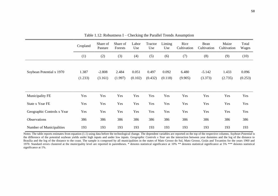
58

Table 1.12: Robustness I – Checking the Parallel Trends Assumption

Cropland

Share of

Pasture

Share of

Forests

Labor

Use

Tractor

Use

Liming

Use

Rice

Cultivation

Bean

Cultivation

Maize

Cultivation

Total

Wages

(1) (2) (3) (4) (5) (6) (7) (8) (9) (10)

Soybean Potential x 1970 1.387 -2.808 2.484 0.051 0.497 0.092 6.480 -5.142 1.433 0.096

(1.233) (3.161) (1.997) (0.102) (0.432) (0.118) (9.905) (3.373) (2.735) (0.253)

Municipality FE Yes Yes Yes Yes Yes Yes Yes Yes Yes Yes

State x Year FE Yes Yes Yes Yes Yes Yes Yes Yes Yes Yes

Geographic Controls x Year Yes Yes Yes Yes Yes Yes Yes Yes Yes Yes

Observations 386 386 386 386 386 386 386 386 386 386

Number of Municipalities 193 193 193 193 193 193 193 193 193 193

Notes: The table reports estimates from equation (1.1) using data before the technological change. The dependent variables are reported on the top of the respective columns. Soybean Potential is

the difference of the potential soybean yields under high inputs and under low inputs. Geographic Controls x Year are the interaction between year dummies and the log of the distance to

Brasília and the log of the distance to the coast. The sample is composed by all municipalities in the states of Mato Grosso do Sul, Mato Grosso, Goiás and Tocantins for the years 1960 and

1970. Standard errors clustered at the municipality level are reported in parentheses. * denotes statistical significance at 10% ** denotes statistical significance at 5% *** denotes statistical

significance at 1%.

59

Table 1.13: Robustness II – Additional Controls for Agricultural Outcomes

Price Controls Land Tenure Access to Credit

Cropland Tractor

Use

Crop

Output Cropland

Tractor

Use

Crop

Output Cropland

Tractor

Use

Crop

Output

(1) (2) (3) (4) (5) (6) (7) (8) (9)

Soybean Potential x 1975 1.930** 0.178** 0.275** 1.503 0.151* 0.195* 1.797* 0.159** 0.237**

(0.938) (0.078) (0.110) (0.922) (0.079) (0.111) (0.943) (0.078) (0.110)

Soybean Potential x 1980 4.186*** 0.390*** 0.419*** 3.535*** 0.350*** 0.295** 4.014*** 0.363*** 0.367***

(0.966) (0.101) (0.123) (0.933) (0.103) (0.130) (0.967) (0.101) (0.131)

Soybean Potential x 1985 5.404*** 0.584*** 0.534*** 4.596*** 0.541*** 0.386*** 5.281*** 0.561*** 0.489***

(1.067) (0.129) (0.138) (1.024) (0.134) (0.146) (1.083) (0.132) (0.148)

Municipality FE Yes Yes Yes Yes Yes Yes Yes Yes Yes

State x Year FE Yes Yes Yes Yes Yes Yes Yes Yes Yes

Geographic Controls x

Year Yes Yes Yes Yes Yes Yes Yes Yes Yes

Baseline Controls x Year Yes Yes Yes Yes Yes Yes Yes Yes Yes

Observations 1,016 1,016 1,016 1,016 1,016 1,016 1,016 1,016 1,016

Number of Municipalities 254 254 254 254 254 254 254 254 254

Notes: The table reports estimates from equation (1.1) in the text. The dependent variables are reported on the top of the respective columns. Cropland is the share of farmland cultivated with

crops. Tractor Use is the number of tractors per thousand hectares of farmland. Crop Output is the log of the value of crop output per labor unit. Soybean Potential is the difference of the

potential soybean yields under high inputs and under low inputs. Geographic Controls x Year are the interaction between year dummies and the log of distance to Brasília and the log of distance

to the coast. Baseline Controls x Year are the interaction between year dummies are the baseline value of the share of available land, the log of the number of farms, the log of total farmland, the

number of state-owned bank branches, the number of private bank branches and the dependent variable. The sample is composed by all municipalities in the states of Mato Grosso do Sul, Mato

Grosso, Goiás and Tocantins for the years 1970, 1980 and 1991. Standard errors clustered at the municipality level are reported in parentheses. * denotes statistical significance at 10% **

denotes statistical significance at 5% *** denotes statistical significance at 1%.

60

Table 1.14: Robustness II – Additional Controls for Population Outcomes

Price Control Land Tenure Access to Credit

Primary

Schooling

(0/1)

Skilled

Occupation

(0/1)

Primary

Schooling

(0/1)

Skilled

Occupation

(0/1)

Primary

Schooling

(0/1)

Skilled

Occupation

(0/1)

(1) (2) (3) (4) (5) (6)

Soybean Potential x 1980 0.034*** 0.009* 0.033*** 0.008* 0.032*** 0.010**

(0.009) (0.004) (0.009) (0.004) (0.009) (0.004)

Soybean Potential x 1991 0.059*** 0.020*** 0.052*** 0.017*** 0.054*** 0.023***

(0.012) (0.006) (0.012) (0.006) (0.012) (0.006)

Municipality FE Yes Yes Yes Yes Yes Yes

State x Year FE Yes Yes Yes Yes Yes Yes

Geographic Controls x Year No Yes Yes No Yes Yes

Baseline Controls x Year No No Yes No No Yes

Observations 453,187 447,154 453,187 447,154 453,187 447,154

Number of Municipalities 254 254 254 254 254 254

Notes: The table reports estimates from equation (1.2) in the text. The dependent variable is reported on the top of the respective columns. The sample includes individuals with 15-64 years old,

living in rural areas and either working or looking for a job. Soybean Potential is the difference of the potential soybean yields under high inputs and under low inputs. Geographic Controls x

Year are the interaction between year dummies and the log of distance to Brasília and the log of distance to the coast. Baseline Controls x Year are the interaction between year dummies are the

baseline value of the share of available land, the log of the number of farms, the log of total farmland, the number of state-owned and private bank branches and average value of the dependent

variable in the municipality. The sample is composed by all municipalities in the states of Mato Grosso do Sul, Mato Grosso, Goiás and Tocantins for the years 1970, 1980 and 1991. Standard

errors clustered at the municipality level are reported in parentheses. * denotes statistical significance at 10% ** denotes statistical significance at 5% *** denotes statistical significance at 1%.

2 Geographic Heterogeneity and Technology Adoption: Evidence from the Direct Planting System

2.1. Introduction

Low adoption of modern agricultural technologies is considered an

important constraint to agricultural development across the developing world.24

This phenomenon is associated with several possible explanations, ranging from

market failures to behavioral biases.25

This paper documents another determinant

of under-adoption of modern agricultural technologies: geographic heterogeneity.

Diamond (1997) suggests that the distribution of geographic characteristics

can affect agriculture through its influence on technology adoption. The author

writes that “among all those areas where food production did spread in the

prehistoric era, the rates and dates of spread varied considerably. At the one

extreme was its rapid spread along east-west axes: (...) At the opposite extreme

was its slow spread along north-south axes. (...) Localities distributed east and

west of each other at the same latitude share exactly the same day length and its

temporary variations. To a lesser degree, they also tend to share similar diseases,

regimes of temperature and rainfall, and habitats or biomes."26

However, the

existing literature focuses on the impact of the level of geographic characteristics

on agricultural development, being silent on the effects of the variation in

geographic characteristics on agricultural development.27

This paper provides evidence that low adoption of modern technologies in

agriculture can be related to geographic heterogeneity using data from the

utilization of the Direct Planting System (DPS) in the Brazilian agriculture. Using

24

Estimates indicate that returns to the adoption of modern agricultural technologies are quite

high (Duflo et al., 2008; Suri, 2011). 25

Foster and Rosenzweig (1995) and Conley and Udry (2010) emphasize the role of social

learning to technology adoption in India and Ghana. Karlan et al. (2014) investigates the role of

market failures to investments and technology adoption in Ghana. Suri (2011) emphasizes the role

of comparative advantage in explaining under-adoption of modern technologies in agriculture in

Kenya. Duflo et al. (2011) investigates the role of behavioral biases in explaining adoption

decisions among Kenyan farmers. 26

See Diamond (1997), p. 178 and p. 183. 27

See, for instance, Hornbeck (2012) and Hornbeck and Keskin (2014).

62

soil heterogeneity as a measure of geographic heterogeneity, we present evidence

that it has a negative effect on the adoption rate of the DPS.

We propose a simple theoretical model connecting geographic heterogeneity

and technology adoption through adaptation costs. In the model, adaptation costs

increase and adoption becomes more difficult when farmers observe successful

adoption experiences under different geographic conditions.28

That leads to lower

equilibrium adoption rates in economies in which geographic heterogeneity is

high. In addition to that, the model predicts that the impact of soil heterogeneity

should be zero when adoption rates are either too low or too high. In the former

case, adaptation cannot take place because there are not enough adopters to learn

from. In the latter, the new technology is so widespread that most farmers will

find a neighbor operating under similar geographic conditions regardless

geographic heterogeneity. For intermediate adoption levels, the model predicts the

impact of heterogeneity to be highest.29

In the model, the presence of adaptation costs affects the format of the

relationship between adoption levels and geographic heterogeneity. This pattern

can be used to evaluate the presence of adaptation costs using indirect evidence.

That is important when direct information is hard or impossible to collect.30

In

addition, the model predicts that the relationship between geographic

heterogeneity and technology adoption should hold in all periods, allowing the use

of cross-sectional data in the empirical investigation.

The model is tested using detailed data on soil characteristics and

information on technology adoption of the Direct Planting System (DPS). The

DPS was developed in southern Brazil in the 1970s based on previous experiences

28

An alternative explanation is based on the informational content of experiences performed

under different conditions (see, for example, Munshi (2004)). Although this interpretation leads to

the same results, we opt for the adaptation costs view as it is more suitable to the actual diffusion

process of the DPS in Brazil. 29

It should be noted that this non-monotonic pattern is related to the traditional S-curve which

depicts adoption levels over time: it is nearly flat when adoption levels are either too low (as there

are few adopters to be imitated) or too high (when there are few non-adopters to imitate). Although

driving forces are not exactly the same, a non-monotonic behavior also arises: the derivative of the

S-curve is increasing within a given range and then starts decreasing. The present model captures a

similar effect over quantiles of the unconditional distribution of adoption. See the chapter 7 in

Jackson (2008) for a theoretical discussion of the S-curve. Foster and Rosenzweig (1995) estimate

that adoption of modern technologies in agriculture follows the S-curve. 30

In a similar vein, Young (2009) explores differences in the adoption rates over time (known

as the S-curve) to identify social learning as the actual diffusion channel of a new technology.

63

with no-till farming.31

It was developed in areas prone to land degradation. It later

evolved into a full farming method with higher revenues and lower costs than the

traditional (tillage-based) methods. Inoue (2003) reports that DPS adoption is

associated with costs 9% lower and with revenues 17% higher in the case of

soybean cultivation.32

The limited use of tillage also prevents soil degradation and

the loss of nutrients due to plowing, increasing long-run productivity.33

The DPS has two essential features for the analysis. First, adoption

configures an actual technological innovation and does not require large changes

in input use. It mainly requires learning about the new way of combining inputs

for production and minor modifications in machinery. Second, other constraints to

technology adoption are absent. Credit constraints are not relevant as there are no

upfront costs, while risk does not seem to be an issue since the DPS decreases risk

exposure. There is also no need for additional infrastructure and scale issues do

not appear to be relevant as adoption rates are similar across farm sizes.34

Despite these features, only 10.1% of the Brazilian farmers adopted the DPS

in 2006. The agronomic literature attributes under-adoption of the DPS to lack of

knowledge since the practice must be adapted to different geographic conditions

to function well. Sorrenson and Portillo (1997) state that the adoption of no-tillage

techniques “necessitates the learning and mastering of an array of new crop

management skills”. Derpsch (1999) argues “site specific knowledge of the no-

tillage system has most likely been the main limitation to the spread of the system

in (...) Latin America”. Therefore, the DPS have features suggesting that the

negative relationship between geographic heterogeneity and technology adoption

can be interpreted as evidence of the relevance of adaptation costs.

We use both detailed GIS data on soil characteristics and data from the 2006

Brazilian Agricultural Census to examine the relationship between geographic

heterogeneity and DPS adoption. We choose soil heterogeneity to be the relevant

31

No-tillage refers to any way of preparing the soil for planting in which tillage is limited or

even absent and crop residue is left on the surface. 32

See Sorrenson and Portillo (1997) and Trigo et al. (2009) for evidence on DPS benefits in

other South American countries. 33

The DPS adoption is also associated to an increase in carbon sequestration and a reduction

in greenhouse gas emissions in agriculture. These environmental benefits have been documented

in several setting. See Tesla et al. (1992), West et al. (2002), and Metay et al (2007) for some

evidence on these gains. 34

Detailed accounts of these features of the DPS can be found in Landers (2005) and Derpsch

et al. (2010).

64

geographic heterogeneity measure because soils affect how the DPS should be

used. The composition of each soil affects physical properties like temperature.

These properties affect the implementation of the DPS. For example, a higher soil

temperature calls for a thicker layer of residue on the surface.

We measure soil heterogeneity using a physicochemical classification of

soil types that is invariant to land use. We use this classification to construct the

share of the municipal area covered with each soil. These shares are used to build

a Herfindahl index (HHI) and the inverse of this index is used as the heterogeneity

measure. It is important to notice that this measure does not have a direct impact

on farming as it does not affect agricultural output or the use of other inputs.35

Using a sample of Brazilian municipalities, we estimate that soil

heterogeneity reduces DPS adoption even when controlling for the several

geographic characteristics (soil types, rainfall, temperature, land gradient, altitude,

latitude and longitude) and socioeconomic characteristics (education, number of

farms, farm revenues, government technical assistance and state fixed effects).

The estimated impact is meaningful: an increase in one standard deviation in soil

heterogeneity decreases DPS adoption in 1 to 1.3 percentage points. The results

are robust to the inclusion of measures of land use, cooperatives and access to

credit as additional controls. Results are also robust to changes in sample

definition.

Placebo tests provide evidence that soil heterogeneity neither influences the

adoption of non-agricultural technologies (such as electricity) nor the adoption of

technologies related to harvesting (such as the combine harvester). These tests

provide suggestive evidence that adaptation cost mechanism proposed in the

theoretical model.

Further investigation of the proposed mechanism is done using an

unconditional quantile regression estimator suggested by Firpo et al. (2009). The

estimator uses a regression approach based on Recentered Influence Functions

(RIF) to estimate the impact of soil heterogeneity across different quantiles of the

adoption distribution. This method enables us to test if the effect of soil

heterogeneity on DPS adoption is non-monotonic as the theoretical model

35

We choose this measure because it has a simple interpretation. The inverse of the HHI index

is a measure of the effective number of soils. However, the literature suggests some alternative

measures. See, for instance, Esteban and Ray (2011) for a discussion of alternative measures in an

investigation between ethnic fractionalization and conflict.

65

predicts. Results are consistent with the theoretical model. The effect of soil

heterogeneity is higher than the average impact when adoption rates range from

20 to 50 percent (percentiles 50 to 75 in the sample). It peaks at an adoption rate

of 40% percent (percentile 70). In this rate, an increase in one standard deviation

in soil heterogeneity reduces DPS adoption by 4.5 percentage points.

These results contribute to two fields of the literature. First, it contributes to

the strand that investigates the relationship between geographic characteristics and

economic outcomes. A substantial literature documents the impact of geography

on determinants of economic development such as historical institutions, ethnic

fractionalization, and cultural formation (Durante, 2010; Michalopoulos, 2012;

Fenske, 2014; Alsan, 2015). We provide evidence that technology adoption is

another channel through which geographic characteristics influences economic

outcomes. Our results support the view that geographic similarities facilitate the

adoption of modern technologies proposed by Diamond (1997).

Second, we contribute to the literature on the determinants of under-

adoption of modern technologies in agriculture. The literature stresses the

importance of formal training (including educational levels) and social learning in

technology adoption (Foster and Rosenzweig, 1995; Munshi, 2004; Bandiera and

Rasul, 2006; Conley and Udry, 2010). The literature also stresses that market

failures in credit and insurance markets reduce technology adoption in agriculture

due to significant setup costs and risks often involved in the adoption of modern

technologies (Udry, 2010; Karlan et al., 2014). We provide evidence that

geographic heterogeneity can also reduce technology adoption.36

The remaining of the paper is organized as follows. Section 2 describes the

Direct Planting System and its diffusion in Brazil. Section 3 presents the

theoretical model. Section 4 describes the data. Sections 5 report the main

estimates and robustness tests. Section 6 reports the unconditional quantile results.

Section 7 concludes.

36

Comin and Ferrer (2013) provide evidence that a large part of income inequality among

countries can be explained by technology penetration rates (while adoption lags have converged).

Our paper suggests that these rates may be affected by geographic heterogeneity.

66

2.2. Historical Background

2.2.1. Overview of the Direct Planting System

The DPS is a no-till technique developed in Brazil at the beginning of the

1970s. These techniques can be described as agricultural practices in which tillage

is limited or absent and crop residue is left on the surface. Soil is then preserved:

loss of nutrients due to plowing and rain erosion decrease. However, the use of

no-till techniques in large-scale agriculture is only possible when effective

herbicides are available as tillage is an important tool for weed control.

The no-till techniques challenge a long established notion in agriculture: the

importance of tillage. The plow can be considered one of the main historical

determinants of agricultural development as it facilitated weed control. The

development of plows capable of inverting soil layers in the 17th century and

other subsequent technological advances made tillage even more important and

contributed to a significant increase in food production. As Derpsch (1997) put it,

“because the modern plow saved Europe from famine and poverty it became a

symbol of “modern” agriculture (...). Colonies in America, Asia and Africa simply

followed the European pattern”.

The plow's substantial gains in terms of weed control and soil scarification

meant that it was worth using it despite its cost in terms of land degradation and

erosion. Indeed, modern no-till techniques were developed just after the 1940s

when herbicides became more efficient. The development of more effective forms

of weed control in the following decades triggered more research on no-till

techniques. These techniques have become a popular feature among proponents of

sustainable agricultural practices (Baker et al., 2007).

The DPS is a particular no-till method in which absence of tillage is

permanent and the use of green manure crops to cover the soil is widespread

(Derpsch et al., 2010). Both features resulted from the effort to adapt no-till

techniques to the specific geographic conditions Brazilian farmers faced. This

technique has become popular in other countries in South America as well.

The adoption of the DPS characterizes the adoption of a novel production

technology as adopters continue to use similar the same inputs to obtain higher

output. It can thus be characterized as the adoption of a different production

process that uses the same inputs (as opposed to the adoption of formerly

67

underused inputs in the same production process).37

This is an important feature

of the technique for the empirical investigation since it is often difficult to

separate adoption from input underuse (Foster and Rosenzweig, 2010).

DPS adoption is known for having both public and private gains. Table 2.1

describes the benefits from the technique. Public gains are presented in Panel A

and are unambiguous. These main benefits come both from lower carbon

emissions and higher carbon sequestration. Both changes have positive

externalities to the environment and mitigate climate change (Tesla et al., 1992;

West et al., 2002; Metay et al, 2007). Other gains have been reported in terms of

reduced environmental contamination and increased biodiversity (Derpsch et al.,

2010; Camargo et al., 2011).

Private gains are presented in Table 2.1, panel B. These benefits come from

a combination of higher revenues and lower costs. The DPS reduces soil

degradation and erosion and improves soil properties, resulting in higher

revenues. It also decreases the use of machines to plow the soil. Although

expenditures with fertilizers increase, the costs fall even in the short term

(Derpsch et al., 2010; Baker et al., 2007).

A substantial literature quantifies the economic benefits from the DPS.

Inoue (2003) presents evidence that DPS adoption decreases soybean productivity

in 17% in Brazil. The author also presents evidence that average costs decrease

9% with DPS adoption. Sorrenson and Portillo (1997) reports that DPS increases

net income by 33% in the first year of adoption among farmers in Paraguay. The

authors also argue that the benefit from the DPS increases over time. Trigo et al

(2009) estimates substantial economic benefits from DPS adoption in Argentina

coming both from increases in production and decreases in costs. Ringler et al

(2013) simulates that widespread adoption of no-till techniques would increase

yields of staple crops even considering the effects of climate change on

temperature and rainfall. The authors argue that no-till is a promising farming

techniques to mitigate climate change’s impact on agriculture.

An important feature of the DPS is that neither credit constraints nor

incomplete insurance seem to be barriers to its adoption. First, the technique has

37

The optimal choice of inputs often changes under a new technology. However, this is

different from change of inputs given a technology such as, for example, when credit constraints

are lowered.

68

no upfront costs, suggesting that access to credit is not a constraint for adoption.

Second, the method reduces production risks as input demand decline and yield

volatility decline. This feature suggests that lack of insurance is also not a barrier

to DPS adoption. Furthermore, adoption of the DPS does not require additional

infrastructure and scale issues also seem to be irrelevant since adoption rates are

similar across farm sizes.

Information, on the other hand, appears to be the major barrier to DPS

adoption. Derpsch (1999) describes the adjustments needed to use the technique in

tropical soils that are often “acid or have toxic aluminum”. The author argues that

adjustment required to make the DPS suitable are unique to the type of soil under

consideration (although there are some general practices that must be used in all

contexts). He suggests that lack of “site specific knowledge” has been a

significant barrier to the diffusion of DPS in Latin America. Indeed, his first two

recommendations for farmers willing to adopt such techniques are:

“1- Improve your knowledge about all aspects of the system but especially

in weed control.

2- Analyze your soil. (...)”

2.2.2. The Diffusion of the Direct Planting System in Brazil

Brazil is the fifth largest in the world and agricultural conditions differ

substantially across its regions. The DPS was first implemented at the beginning

of the 1970s in southern Brazil. This region’s main geographic characteristics are

the sub-tropical climate and fertile soils. These features attracted European

immigrants in the late 1800s which compose a large share of the farmers in the

region.

The first tests with the DPS in Brazil happened at the beginning of the

1970s with sorghum and wheat. The technique was developed to fight rain erosion

that affected soils in the region of Ponta Grossa in the state of Paraná. Pioneer

farmers studied no-till techniques abroad and assumed the risk of importing

equipment and knowledge and testing the method on large scale. These farmers

exerted a significant influence on the development of the DPS in Brazil and

induced research on the technology in private institutes as well as public

universities.

69

For instance, the IAPAR (Agronomic Institute of Paraná – a private

institution) started a soil conservation program that promoted the DPS in 1975.

Later Embrapa (the Brazilian Agricultural Research Corporation – a public

institution) also began to influence the development of the DPS. Since its creation,

the technique evolved from a practice to reduce rain erosion to a complete

production method.

Anecdotal evidence suggests that large farmers in the Ponta Grossa region

started adopting the DPS in 1976. The first adopters were concentrated in southern

Brazil, but later the farmers from northern areas started to use the technique.

These northern regions feature diverse tropical environments, in particular in the

Cerrado biome. The first attempts to implement the DPS in this biome happened

in the 1980s. Adoption in the region accelerated since the 1990s.

An important feature of the DPS diffusion was the creation of an association

called Clube da Minhoca38

(henceforth CM) in 1979. The CM is located in Ponta

Grossa and is a diffusion center with the goal of spreading knowledge about the

technique. The organization promoted meetings where farmers (adopters and non-

adopters) would discuss issues related to farming. It also organized national

meetings and sponsored the publication of technical material about the DPS.

The CM inspired the creation of private associations with a similar objective

in other localities. These associations are called Clube Amigos da Terra39

(henceforth CAT) and the first was established in 1982 in the state of Rio Grande

do Sul. These associations were an essential tool for the diffusion of the DPS

throughout Brazil. The CATs coordinate learning efforts and information

exchange among farmers. The CATs and other organizations that promote the

technique were essential to spread information and knowledge about the method.

Indeed, these private organizations seem to have been more important to DPS

diffusion than the public extension services.

However, the presence of these associations was not sufficient to induce

most Brazilian farmers to adopt the DPS. Almost 90% of the farmers did not

adopt the technique despite the substantial increase in adoption since the 1990s

depicted in Figure 2.1. The adoption rate is similar across farm sizes and is higher

in the crop-intensive areas in southern and central Brazil.

38

Translated as “Earthworm club” as the presence of earthworm was a sign of soil vitality. 39

Translated as “Friends-of-the-earth club”.

70

The next section proposes a formal model to deal with the need to adjust the

DPS for different geographic conditions. Notice that such differences have no

direct impact on agriculture as we only analyze soils where agriculture is viable in

the first place under both traditional tillage and DPS. We interpret them as a

barrier to adaptation to different soil types where DPS has not been used before.40

2.3. Model

Consider a simple economy with a continuous mass of farmers with size

normalized to one. Each farmer 𝑖 has a soil 𝜃𝑖 ∈ ℝ𝑁. Soils are distributed

according to a single-peaked joint distribution 𝐺(𝜃; 𝜎2) with associated density 𝑔.

The variance 𝜎2 is assumed to be strictly positive and determines how much soils

differ: soil heterogeneity is captured by a higher 𝜎2. We assume that the

probability that 𝜃𝑖 = 𝜃𝑗 is zero for all 𝑖 ≠ 𝑗.41

There are two technologies available for crop production: a traditional

technology and a new technology. We assume (discounted) profits from the new

technology, 𝜋, are larger than under the current one, 𝜋. Define Δ𝜋 = 𝜋 − 𝜋 > 0.

Despite the difference in profits, farmers might not use the new technology since

there is a non-pecuniary cost to adopt it. In each period 𝑡, the adoption decision is

described by 𝑎𝑖𝑡: 𝑎𝑖𝑡 = 1 if he adopts the new technology and 𝑎𝑖𝑡 = 0 otherwise.

Each farmer 𝑖 is then characterized by a sequence (𝜃𝑖, 𝑎𝑖𝑡)𝑡.

The adoption cost reflects the need to make some adjustments to the new

technology (a micro-innovation) in order to use it in a different type of soil. We

assume that this cost will be lower when the farmer has neighboring farmers who

adopted the technology. This assumption captures the intuition that farmers can

learn from their peers’ experiences. Therefore, the cost of farmer 𝑖 in period 𝑡

depends on the previous adopter 𝑗 with the most similar type of soil, i.e., it should

depend on min𝑗 𝑑(𝜃𝑖 − 𝑎𝑗𝑡𝜃𝑗), in which 𝑑 is the Euclidean distance.

40

An alternative interpretation is related to the informational content of an experience

performed under different conditions. The agent then updates his prior on the profitability of the

new technology based on the conditions his neighbors were faced with and the results they

achieved. Although the model in the next section is able to accommodate this Bayesian

interpretation, we choose the adaptation cost view as it captures more precisely the features of the

DPS. 41

This is done only for simplicity but its interpretation is straightforward: two types of soil are

never exactly equal even if any differences are irrelevant for the farmer's decision.

71

In order to define this cost for a continuum of farmers, we define the R-

neighborhood of farmer 𝑖 as:

𝑁(𝜃𝑖) = {𝜃𝑗: 𝑑(𝜃𝑖, 𝜃𝑗) ≤ 𝑅} (2.1)

This is the set from which a farmer can learn from. This set has mass

𝑀(𝑁(𝜃𝑖)) = ∫ 𝑔(𝜃)𝑑𝜃𝑁(𝜃𝑖)

. We also define the set of adopters in 𝑖’s

neighborhood in period 𝑡 as:

𝑁𝐴𝑡(𝜃𝑖) = {𝜃𝑗: 𝑑(𝜃𝑖, 𝜃𝑗) ≤ 𝑅 𝑎𝑛𝑑 𝑎𝑗𝑡 = 1} (2.2)

This set has mass 𝑀(𝑁𝐴𝑡(𝜃𝑖)) = ∫ 𝑔(𝜃)𝑑𝜃

𝑁𝐴𝑡 (𝜃𝑖)

. The cost of adaptation 𝑐(. )

is a function of this set. This cost function 𝑐 (𝑀(𝑁𝐴𝑡(𝜃𝑖))) is assumed to have the

following properties:

i. 𝑐(0) > Δ𝜋

ii. 𝑐(. ) is decreasing in its argument and there is 𝑚 < 1 such that 𝑐(𝑚) < Δ𝜋.

Assumption (i) means that the cost of the original innovation is too high: the

farmer will not adopt the new technology if there are no neighbors to adapt from

(and no alternative diffusion channel). Hence, we are modeling the diffusion and

not the initial innovation process.

Assumption (ii) captures the adaptation channel. The presence of adopters in

the R-neighborhood decreases the cost of adaptation as farmers can learn about

the technology by observing other adopters operating close to them. Moreover, the

new technology is viable for a high enough adoption rate in the farmer’s

neighborhood.

The farmers can also have access to some alternative diffusion channel that

reduces adoption costs. This alternative is interpreted as access to formal diffusion

channels as extension services, cooperatives, and dissemination centers. These

channels are labeled 𝐹𝑡 such that 𝐹𝑡 = 0 represents the absence of such channel in

that period. The total cost of adaptation is defined as:

𝑐 (𝑀(𝑁𝐴𝑡(𝜃𝑖))) − 𝐹𝑡 (2.3)

It is important to note that that Δ𝜋 > 0 implies that adopters never switch

back to the base technology: 𝑎𝑖𝑡 = 1 ⟹ 𝑎𝑖𝑡′ = 1 for all 𝑡′ > 𝑡. At the beginning

of every period, non-adopters observe the previous distribution of adoption and

make their decisions. Timing is as follows:

72

𝑡 = 0: exogenous and independent distribution of types (𝜃𝑖) and initial

adopters (𝑎𝑖0) is drawn;

𝑡 = 1: beginning of the period: non-adopters decide whether to adopt or not

the technology based on (𝜃𝑖 , 𝑎𝑖0);

𝑡 = 1: end of the period: new distribution of adopters is observed by all

agents;

𝑡 = 2: beginning of the period: non-adopters decide whether to adopt or not

the technology based on (𝜃𝑖 , 𝑎𝑖1);

And so forth.

An agent will adopt the new technology whenever the gain in profit is

higher than the cost of adaptation. Therefore, a farmer 𝑖 will adopt the technology

in period 𝑡 (𝑎𝑖𝑡 = 1) if:

Δ𝜋 ≥ 𝑐 (𝑀(𝑁𝐴𝑡(𝜃𝑖))) − 𝐹𝑡 (2.4)

Let 𝑀 = 𝑐−1(Δ𝜋). This is the lowest mass of adopters, in a given

neighborhood, that allows diffusion to take place. Define 𝑀𝑈 = 𝑀(𝑁𝐴0(𝜃𝑖)) as the

initial mass of adopters around 𝜃𝑖 under the uniform distribution and notice that is

must be the same for all 𝑖. We further assume that 𝑀 > 𝑀𝑈: if the distribution of

types is uniform, the mass of adopters is too low, in any neighborhood, for

diffusion to take place.42

The intuition is that the initial level of adoption cannot

trigger diffusion if entropy is high enough: the number of adopters at 𝑡 = 0 is not

sufficient to render soil variance irrelevant. This assumption is not essential for

the main results. It is made for the sake of simplicity and is in line with the under-

adoption issue discussed in the previous sections.

Notice that this diffusion process cannot be reduced to a contagion model: it

is not enough to have adopters in the neighborhood. In the presence of operational

differences in the use of the new technology among different soils, it is necessary

to incur a cost to adjust it. This cost is by construction lower when previous

adopters operate under similar conditions as non-adopters.43

42

This assumption is trivially satisfied if the support of types is unbounded. If 𝜃 ∈ ℝ this

assumption boils down to 𝑀 > 2𝑅𝛼. 43

It is possible to rewrite the model in terms of learning about profits instead of how to

operate the technology.

73

Decisions in period 𝑡 induce a (possibly changed) end-of-period distribution

of adopters with associated mass 𝑀(𝑁𝐴𝑡(𝜃𝑖)). We are implicitly assuming that

farmers need at least one period to adapt the new technology (intuitively, they

have to observe a whole growing cycle). We have 𝑀(𝑁𝐴𝑡(𝜃𝑖)) ≥ 𝑀(𝑁𝐴

𝑡−1(𝜃𝑖)) as

the set of adopters never decreases.

An allocation is a vector of adoption decisions {𝑎𝑖}𝑖𝑡. An equilibrium path is

defined as follows.

Definition 1: For a given vector 𝜃 and initial distribution {𝑎𝑖}𝑖0, an

equilibrium profile {𝑎𝑖∗}𝑖

𝑡 is such that for all 𝑖 and for all 𝑡 ≥ 1, 𝑎𝑖𝑡∗ = 1 if and only

if equation (2.4) holds.

In the long run, this path will converge to {𝑎𝑖∗}𝑖 as it is a bounded and

monotone sequence. Define the set of adopters by Θ𝐴𝑡 and the share of adopters by

𝐴𝑡.

The expected level of 𝐴𝑡 should depend on 𝜎2 for all 𝑡. More dispersion in

soils reduces the likelihood that a farmer will find enough adopters in the

neighborhood to make adoption profitable. However, the impact will depend on

the adoption level 𝐴𝑡 as the following proposition establishes. We assume that the

derivative 𝜕𝐴𝑡 𝜕𝜎2⁄ exists.44

Proposition 1: For any 𝑡, the aggregate adoption level 𝐴𝑡 is constant in 𝜎2

if 𝐴𝑡 = {0,1} and decreasing for some 𝐴𝑡 ∈ (0,1).

Proof. Consider an initial situation in which 𝑎𝑖 = 0 for all 𝑖. Assumption 1

implies that no agent finds profitable to adopt the modern technology. Adaptation

cannot take place in the absence of adopters in the neighborhood. Therefore,

𝐴𝑡(𝜎2) = 0 and 𝜕𝐴𝑡 𝜕𝜎2⁄ = 0. Reasoning is similar for a profile {𝑎𝑖∗}𝑖 such that

𝑀(𝑁𝐴(𝜃𝑖)) > 𝑚 for all 𝑖. Assumption 2 implies that all agents find profitable to

adopt the modern technology. Therefore, 𝐴𝑡(𝜎2) = 1 and 𝜕𝐴𝑡 𝜕𝜎2⁄ = 0. To

prove that 𝜕𝐴𝑡 𝜕𝜎2⁄ < 0 for some intermediate value, it suffices to prove that a

higher variance will lead to lower adoption in the initial period (𝑡 = 1). It follows

that adoption will be lower in all subsequent periods as non-adopters will have a

lower mass of adopters to learn from. Since 𝐺 is single-peaked and 𝑀 > 𝑀𝑈, the

set of farmers such that adoption is profitable decreases when 𝜎2 increases.45

44

It is straightforward to rewrite the argument for a non-differentiable function 𝐴𝑡. 45

It is possible to show that if 𝐺 is not single-peaked, 𝐴𝑡 decreases non-monotonically in 𝜎2.

74

Intuition is straightforward. When adoption levels are too low, there is no

one from whom to learn and adapt the new technology and diffusion cannot take

place at all. It follows that the impact of heterogeneity on adoption is zero. When

adoption levels are high enough, the cost of adaptation becomes lower than the

benefit. Adoption will be so widespread that farmers will be able to adapt no

matter how different their soils are.46

Nevertheless, at intermediate levels, an

increase in heterogeneity must reduce adoption. The level of adopters in any given

neighborhood goes below the minimum needed to allow adaptation.

Without further structure on the distribution 𝐺, one cannot derive additional

properties of 𝜕𝐴𝑡 𝜕𝜎2⁄ . For illustration purposes, assume from that 𝐴𝑡(𝜎2) is

continuously differentiable and has one local minimum labeled 𝐴𝑐. These

assumptions facilitate the interpretation of the empirical results. The following

result is then immediate.

Corollary 1: The derivative 𝜕𝐴𝑡 𝜕𝜎2⁄ is increasing for 𝐴𝑡 ∈ (0, 𝐴𝑐) and

decreasing for 𝐴𝑡 ∈ (𝐴𝑐, 1).

We now turn to the relationship between adaptation costs and other

diffusion channels.

Corollary 2: An increase in the use of the formal channel 𝐹𝑡 can either

crowd out or reinforce the adaptation channel.

These institutions can either weaken or strengthen the relationship between

soil heterogeneity and adoption of the new technology. The formal channel causes

adaptation costs to decrease and thus corresponds to an exogenous increase in the

share of adopters in any given period: 𝐴𝑡 rises. Since the impact of heterogeneity

on adoption is non-monotonic, this adoption rate can be associated either to a

higher impact or a lower one. In the former case, formal channels substitute

adaptation and thus weaken this relationship. In the latter, these alternative

learning mechanisms complement adaptation.

Notice that this result does not rely on any assumption of the cross

derivative of adaptation costs on 𝑀 and 𝐹 which is zero in the present setup. Were

it positive (negative), the region where 𝐹𝑡 and adaptation were substitutes would

be larger (smaller). However, there will be no qualitative change in the results.

46

We are implicitly using the fact that there are no "isolated types". The argument may be

extended to include such cases.

75

The empirical counterparts of the economies described in the model are

municipalities. The variables (𝜎2, 𝛼, 𝑅, 𝐺) describe these economies. The model

predicts that municipalities with higher soil heterogeneity 𝜎2 should have (on

average and for any given 𝑡) lower adoption rates of the DPS. Moreover, this

impact should be zero when these rates are either too low (𝐴𝑡 close to zero) or too

high (𝐴𝑡 close to one). Therefore, the model suggests a specific format for the

relationship between soil heterogeneity and technology adoption. This format is

related to the adaptation costs mechanism and can be used to infer the presence of

this channel.

It is worth stressing that the predictions above hold at an aggregate level and

can be tested without using individual-level data. However, it is also worth

emphasizing that farmers are heterogeneous within and across Brazilian

municipalities in several dimensions not considered in the model. Both profits and

adaptation costs might be correlated with farmers’ characteristics, being an

important challenge for estimation to control for these characteristics.

2.4. Data

2.4.1. Soil Heterogeneity

We build the soil heterogeneity measure using detailed GIS information

from a Brazilian soil map developed by Embrapa, the Brazilian Agricultural

Research Corporation (Embrapa, 2011). The data is based on an international soil

classification system (Santos, 2006). This classification uses a hierarchical

taxonomy: a hypothetical soil 'Aa1' belongs to order 'A', suborder 'a', group '1'.

'Order' is the first and more general classification level and the following ones are

subdivisions. Although the classification system allows for finer levels, the map

does not report information beyond the third level. Information is at scale

1:5.000.000 for each level.

The classification system is based on soils’ physicochemical composition.

This composition is a major determinant of the physical properties of each type of

soil. Physical properties, in their turn, define the suitability for different

agricultural methods. For example, in the case of the DPS, higher soil temperature

often calls for a thicker layer of residue on the surface in order to decrease

exposure to sunlight and avoid excessive heat. Hence, a different type of soil calls

76

for some adjustment (a micro-innovation) in the use of the DPS. This

classification system is “smooth” in the sense that, for agricultural purposes, the

difference in physical properties between two soils is roughly the same for soil

pair.

The baseline empirical specification considers the most general level (order)

to construct the soil heterogeneity measure. This level has the advantage of being

invariant to the agricultural method in use. Although different practices may either

enrich or impoverish the soil by affecting the levels of several nutrients, this

process cannot go as far as to change its basic chemical structure. Therefore,

measures built using this level can be assumed not to depend on the adoption of

the DPS or of other agricultural practices. We provide evidence in the robustness

section that results are unchanged when one considers the more refined levels (a

natural result since the correlation between alternative soil heterogeneity measures

is quite high).

There are 35 different orders across Brazil. We merge the soil map with the

map of municipalities to build a measure of the share of each municipality

covered by each soil order. We use the same procedure to build measures for the

other levels. These shares are used to construct a Herfindahl index (HHI) of soil

types for each municipality. The index varies from zero to one with a higher value

denoting more homogeneity.

Soil heterogeneity (𝑆) is defined as the inverse of its Herfindahl index

(1/𝐻𝐻𝐼). We interpret it as a measure of the effective number of soils (in line

with the industrial organization literature). 𝑆 is a variance measure and is a direct

empirical counterpart of the variance of soils defined in the theoretical model. We

choose this measure because it is simple to interpret. Nevertheless, it is important

to highlight that other literatures suggest the use of alternative measures.47

We expect a higher 𝑆 to reduce adoption of the DPS. We also expect the

impact of 𝑆 on DPS adoption to be non-monotonic and higher at intermediate

adoption rates. The intuition is that neighbors' experiences are less informative in

more heterogeneous municipalities: adaptation costs are larger and adoption

decreases. Notice that this result is independent of 𝑆 having an impact on

47

See Esteban and Ray (2011) for an example.

77

agricultural output. Indeed, it is worth stressing that 𝑆 is an artificial variable with

no direct impact on production.

Table 2.2 presents summary statistics to the main soil heterogeneity

measure. We trim the upper one percent tail of the heterogeneity distribution as S

increases too rapidly after this threshold. The average value of 𝑆 is 1.67 with

variance 0.64. This means that the average municipality is covered by 1.67 soil

orders.

It is important to note that our approach for measuring heterogeneity in

growing conditions contrasts with Munshi’s (2004) learning study. The author

classifies regions as more or less heterogeneous using information on the crops

cultivated in each of them. He argues that rice growing areas present more

geographic heterogeneity than wheat growing ones and that this pattern influences

technology diffusion. Our approach uses direct geographic information and is

more similar to the approach of Michalopoulos (2012) and Fenske (2014) who

correlate similar measures to historical and institutional development.

2.4.2. Agricultural Outcomes

Data on agricultural outcomes is drawn from the 2006 Brazilian

Agricultural Census. The main agricultural outcome used in our empirical

exercises is the Direct Planting System adoption rate. We define it as the share of

farms that use the DPS. We restrict the baseline estimates to municipalities with

adoption levels above 5% to ensure that we are investigating adoption in

municipalities in which the DPS is viable. The results are robust to including

municipalities below this threshold. We also drop the upper one percent tail of the

soil heterogeneity. We have a final sample of 1,628 municipalities.

Table 2.3 reports the distribution of adoption rates in the restricted sample.

The average adoption rate is 30% (standard deviation equal to 26.5%). Adoption

rates are above 40% in the states in the South of Brazil (Rio Grande do Sul, Santa

Catarina, and Paraná) and approximately 20% in the states in Central Brazil

(Goiás, Mato Grosso do Sul, and Mato Grosso). These are the states that

concentrate most soybean production that is the crop under for which adoption

rates are higher. Adoption rates are around 10% in the other states.

Other agricultural outcomes are used as controls in the empirical analysis.

The agricultural outcomes used are the number of farms, average farm revenues,

78

schooling measures, access to government technical assistance, number of

tractors, association to cooperatives, use of credit, and land distribution measures.

Table 2.2 reports summary statistics for these variables.

2.4.3. Other Variables

The empirical specifications include several other geographic and

socioeconomic variables as controls. Average temporary rainfall and temperature

for the period 1970 to 2010 are calculated for each observation using gridded data

on rainfall and temperature obtained from the Terrestrial Air Temperature and

Precipitation Version 3.01. Rainfall is measured in millimeters of precipitation,

while temperature is measured in Celsius degrees. Land gradient is computed

using raster data from the 90-meter Shuttle Radar Topography Mission (SRTM)

radar. The raster data was used to construct the average land gradient for the

Brazilian municipalities using GIS software (ArcMap 10.1). The gradient is

measured in degrees.

The distance to the nearest diffusion center (CAT) is calculated using the

distance between municipalities' centroids. The distance is calculated in

kilometers. Administrative data on the location of bank branches obtained from

the Brazilian Central Bank is used to calculate the number of bank branches in

each observation. We calculate the number of Banco do Brasil and non-Banco do

Brasil bank branches since this financial institution is the principal supplier of

rural credit in Brazil. Latitude, longitude and altitude were obtained through the

Ipeadata website. Table 2.2 reports summary statistics for these variables.

2.5. Soil Heterogeneity and Technology Adoption

2.5.1. Baseline Results

We begin examining whether soil heterogeneity reduces technology

adoption as predicted by the theoretical model. We test this relationship using the

following specification:

𝐴𝑚𝑠 = 𝛽𝑆𝑚𝑠 + 𝑿𝑚𝑠Γ + δs + 𝑢𝑚𝑠 (2.5)

where 𝐴𝑚𝑠 is the share of farmers who adopt the Direct Planting System and

𝑆𝑚𝑠 is the inverse of the Herfindahl index of soil heterogeneity in municipality 𝑚

and state 𝑠. 𝑿𝑚𝑠 is a vector of controls that includes geographic characteristics

79

and other relevant determinants of technology adoption in agriculture and 𝛿𝑠

represents state fixed effects.

Causal interpretation of the estimated 𝛽 from equation (2.5) relies on the

assumption that soil heterogeneity is uncorrelated with unobserved factors that

might influence technology adoption. Soil heterogeneity may be correlated with

the level of geographic characteristics and these characteristics may influence

adoption. Therefore, we include several geographic characteristics as controls to

mitigate the concern that the level geographical characteristics drive the results.48

The interpretation of the coefficient on soil heterogeneity based on the

assumption that soil heterogeneity does not affect technology adoption through

channels other than adaptation costs. We add several socioeconomic

characteristics as controls to mitigate the concern that socioeconomic

characteristics correlated both with soil heterogeneity and technology adoption are

driving the result. We provide evidence that results are robust to the choice of

socioeconomic controls.49

Table 2.4 presents the baseline estimates. Column 1 reports the results from

the regression of the DPS adoption rate on soil heterogeneity conditional on the

level of several geographic characteristics. Controls included are the share of the

municipality covered by each soil type, historical temperature and rainfall in each

season, latitude, longitude and land gradient. The coefficient on soil heterogeneity

is significantly negative which implies that soil heterogeneity reduces the

adoption rate as predicted by the theoretical model. The coefficient suggests that

an increase in one standard deviation in soil heterogeneity (0.69 in the sample)

reduces the DPS adoption rate by 1.1 percentage point.

Column 2 includes state fixed effects as controls. The fixed effects aim to

capture for unobserved socioeconomic characteristics that might change at the

state level. The coefficient on soil heterogeneity is significantly negative and its

absolute value increases.

48

Another concern would be reverse causation. However, the soil classification used to

construct the soil heterogeneity measure is insensitive to land use and, therefore, reverse causation

is not a relevant issue to the estimation. 49

Notice that causal inference is unaffected by the inclusion of socioeconomic characteristics

as additional controls since soil heterogeneity is invariant to socioeconomic characteristics. The

inclusion of socioeconomic characteristics assesses the “adaptation cost” mechanism proposed in

the theoretical model.

80

In column 3 we further includes farm characteristics as additional controls.

The inclusion of these controls tests whether the results are caused by the

correlation between soil heterogeneity and socioeconomic determinants of DPS

adoption. The controls included are the log of the number of farms, the log of

farm revenues, the share of farmers who completed high school, the share of

farmers with access to government provided technical assistance, and log of the

number of tractors. The coefficient on soil heterogeneity remains similar both in

magnitude and significance. Its magnitude implies that an increase in one standard

deviation in soil heterogeneity (0.67 in the sample) reduces the DPS adoption rate

by 1.4 percentage points.50

The results from columns 1 to 3 provide support to the idea that adaptation

costs are the mechanism connecting higher soil heterogeneity and lower

technology adoption. The results also suggest that some important farm

characteristics such as revenues, schooling and access to government provided

technical assistance are not correlated with technology adoption (conditional on

the geographic controls). That suggests that neither capital nor formal training are

constraints to DPS adoption.

The baseline estimates are consistent with the theoretical model and provide

evidence that geographic heterogeneity reduces technology adoption. Our results

suggest that under-adoption of modern technologies in agriculture can be an issue

in heterogeneous areas whenever adaptation costs are present.

An important question is whether the presence of other learning channels

mitigates the impact of geographic heterogeneity on technology adoption. It

should be noted that the theoretical model suggests that other learning channels

such as cooperatives or diffusion centers can either increase or decrease the

impact of soil heterogeneity on adoption rates. The intuition for this result is

50

A common problem in inference when using data on quite small spatial units is the presence

of spatial correlation in the error term. This usually makes standard errors as the ones reported in

Table 4 inconsistent. Therefore, we also estimate the standard errors using the method proposed by

Conley (1999). The method allows estimation of consistent standard errors in the presence of

spatial correlation by imposing some structure to the correlation of the error term across spatial

units using their relative distance. A key feature of the method is deciding a cutoff above which

the correlation falls to zero. We calculate standard errors allowing for spatial correlation of the

error term using three different cutoffs for the distance between municipality centroids: 50

kilometers, 100 kilometers and 150 kilometers. Standard errors from the soil heterogeneity

coefficient in Columns 1 to 3 increase about 20% when the 50 kilometers cutoff. These standard

errors increase, respectively, about 33% and 65% when the 100 and the 150 kilometers cutoffs are

used. Estimates from the preferred specification in Column 3 are significant at the 5% level when

the first and second cutoffs are used and at the 10% level when the third cutoff is used.

81

straightforward. The presence of a formal channel decreases adaptation costs and

increases in the share of adopters. Since the impact of soil heterogeneity on

adoption is non-monotonic, the new level of adoption may be associated with

either a higher or a lower impact.

We investigate the issue using the information on the presence of

cooperatives and proximity to diffusion centers. Cooperatives are an important

institution in rural Brazil and help farmers to acquire inputs and sell their

products. Cooperatives also help farmers in experimenting with different crop

varieties and fertilizers (Jepson, 2006b). We construct a dummy variable to

indicate whether cooperatives are important for a given municipality. The variable

is 1 when the share of producers associated with cooperatives is above the sample

median and 0 otherwise. Diffusion centers known as CAT are also an important

institution in the dissemination of the Direct Planting System throughout Brazil.51

Its primary task is to spread knowledge on the DPS and adapt it whenever needed.

There were 56 diffusion centers in Brazil in 2006. We construct a dummy variable

to indicate whether diffusion centers are near a given observation. The variable is

1 when the distance to the nearest diffusion center is below the sample median

and 0 otherwise.

We examine whether formal learning channels change the impact of soil

heterogeneity on technology adoption using the following specification:

𝐴𝑚𝑠 = 𝛽1𝑆𝑚𝑠 + 𝛽2(𝑆𝑚𝑠 ∗ 𝐹𝑚𝑠) + 𝛽3𝐹𝑚𝑠 + 𝑿𝑚𝑠Γ + δs + 𝑢𝑚𝑠 (2.6)

where 𝐹𝑚𝑠 is an indicator that denotes the presence of the formal learning

channel.

Table 2.4, column 4 reports the coefficients of the regression of the DPS

adoption rate on soil heterogeneity conditional on the presence of formal learning

channels. The presence of cooperatives and diffusion centers is associated with

higher adoption rates as expected. The presence of formal learning channels might

respond to DPS and its inclusion might bias the coefficient on soil heterogeneity

downwards.52

However, the impact of soil heterogeneity on DPS adoption

estimated in column 4 is quite similar to the coefficient estimated in column 3.

Column 5 investigates the interaction effect of the presence of cooperatives.

The coefficient on soil heterogeneity is zero which implies that soil heterogeneity

51

See Section 2 for a detailed explanation on the role of the CATs. 52

For instance, farmers might create formal learning institutions to learn about the DPS.

82

have no impact on DPS adoption in municipalities where cooperatives are not

relevant. However, the interaction effect is significantly negative which means

that soil heterogeneity decreases DPS use in municipalities where cooperatives are

important. The magnitude of the estimates implies that an increase in one standard

deviation increase in soil heterogeneity decreases DPS adoption by 3.4 percentage

points in municipalities where cooperatives are important.

Column 6 investigates the interaction effect of the proximity to diffusion

centers. The coefficient on soil heterogeneity is negative which implies that soil

heterogeneity decreases DPS adoption even in municipalities located far from

diffusion centers. However, the interaction effect is significantly negative which

suggests that soil heterogeneity decreases DPS adoption more in municipalities

where near diffusion centers. The magnitude of the estimates implies that an

increase in one standard deviation increase in soil heterogeneity decreases DPS

adoption by 4.3 percentage points in municipalities near diffusion centers.53

Table 2.4, column 7 includes both interaction effects. Results are similar to

the ones from columns 5 and 6 from the same table. The estimates provide

evidence that the presence of other learning channels reinforces the impact of soil

heterogeneity on DPS adoption.

2.5.2. Alternative Measures and Samples

We consider the robustness of the baseline results to alternative soil

heterogeneity definitions and samples. First, we consider alternative soil

heterogeneity measures. The measure used in the baseline estimates was

constructed using the most general level of the Embrapa (2011) soil map and

information at the municipality level. The alternative measures based on different

soil classifications and other geographic classifications.

The first alternative measure is constructed with more refined information

from the soil map. The main pitfall of this measure is that more detailed

components of the soil might be affected by land use. However, the measure can

be used to test the robustness of the baseline results to alternative soil

classifications.

53

It is possible to include “distance to the initial adopting region” (i.e., the original innovator)

in this exercise – results are unaffected. This accommodates the alternative view of gravitational

diffusion of knowledge (a recent study is Keller and Yeaple (2013)). We interpret the original

innovator as another diffusion center.

83

The correlation between the original and the variable is 0.83. Table 2.5,

column 1 reports the results from the regression of the DPS adoption rate on soil

heterogeneity conditional on the full set of controls included in column 3 from

Table 2.4. The estimated coefficient on soil heterogeneity changes little (-1.95) in

comparison to the coefficient estimated using the original measure (-2.08).

The second alternative measure of soil heterogeneity is also constructed

using information on soil heterogeneity from neighboring municipalities. The

measure is the weighted average of the soil heterogeneity from the municipality

and its neighbors. Weights are the area of the spatial units. The main pitfall of this

alternative measure is that it creates spatial correlation between the soil

heterogeneity measures from different observations. Therefore, the computed

standard errors should be interpreted with caution. However, the alternative

measure can be used to test the robustness of the baseline results to alternative

geographic classifications.

The correlation between the original and the alternative measure defined

above is 0.62. Table 2.5, column 2 reports the results from the regression of the

DPS adoption rate on soil heterogeneity conditional on the full set of controls

included in column 3 from Table 2.4. The estimated coefficient on soil

heterogeneity increases in absolute value (-5.17) in comparison to the coefficient

estimated using the original measure (-2.08). We calculated standard errors

adjusting for the existence of spatial correlation of the error term as we did with

the baseline estimates. The estimated coefficient is statistically different from zero

at the 1% level whichever distance cutoff we choose. The result suggests that the

original measure understates the relevant soil heterogeneity and ends up

attenuating the impact of soil heterogeneity on DPS adoption. Therefore, we can

consider the evidence based on the original measure as a lower bound of the

impact of soil heterogeneity on DPS adoption.

Second, we consider alternative samples. The baseline estimates exclude

municipalities with low adoption levels. This restriction is consistent with the

theoretical model which suggest that adaptation costs are not relevant when

adoption is non-existent or small. We examine whether the baseline results are

sensitive to sample selection considering alternative samples including either all

Brazilian municipalities with information on the relevant variables or all Brazilian

municipalities in which DPS adoption is positive.

84

Table 2.5, column 3 reports the results from the regression of the DPS

adoption rate on soil heterogeneity conditional on the full set of controls included

in column 3 from Table 2.4 using all observations in the sample. The number of

observations increases to 5,060. The coefficient on soil heterogeneity is

significantly negative as in the baseline estimates. However, its absolute value is

smaller than the estimates from the baseline exercise. It should be noted that a

smaller coefficient is expected since the theoretical model suggests that adaptation

costs and soil heterogeneity are not relevant to the observations included in the

sample. Table 2.5, column 4 repeats the exercise using the municipalities in which

DPS adoption is positive. The coefficient on soil heterogeneity is significantly

negative and similar to the one estimated in the full sample.

2.5.3. Additional Controls

We also consider the robustness of the baseline results to the inclusion of

other controls. The additional covariates are included to examine whether the

relationship between soil heterogeneity and DPS adoption is driven not because

adaptation costs, but because the correlation between soil heterogeneity and some

socioeconomic characteristics.54

First, we consider whether the estimates are robust to the inclusion of

controls for land distribution. Land distribution can be correlated with DPS

adoption to the baseline estimates since it may be easier for larger farms to incur

the adaptation costs needed to adopt the DPS. That is a potential concern to the

extent that soil heterogeneity and land distribution are correlated. In this case, the

baseline estimates might confound the impact of soil heterogeneity through

adaptation costs with the impact of soil heterogeneity through land distribution.

We examine whether this is the case including measures of land distribution

as additional controls. The measures included are the share of farmland covered

by farms of different sizes. Table 2.6, column 1 reports the results. The coefficient

of interest is quite similar to the one estimated in the baseline specification (-1.91

versus -2.08).

Second, we consider whether the estimates are robust to the inclusion of

controls for access to financial services. Access to finance can be correlated with

54

Notice that the baseline specification in column 3 in Table 4 includes some socioeconomic

characteristics related to technology adoption.

85

DPS adoption since it may be easier for farmers to incur with the adaptation costs

needed to adopt the technology. The literature suggests that access to finance can

be significant to explain technology adoption (Karlan et al., 2014). While the

literature on the DPS suggests that access to finance is not relevant to its adoption

since it involves no upfront costs or increased risk, it is useful to account for

access to finance in the estimates.

Table 2.6, columns 2 and 3 include measures of financial access as

additional covariates. Column 2 controls for the number of bank branches. We

account separately for the number of Banco do Brasil bank branches and the

number of other bank branches since Banco do Brasil is the primary provider of

rural credit in Brazil. Column 3 also controls for the average value of farm debt as

another measure of financial access. The number of observations decreases in

column 3 since nine municipalities have no data on farm debts.

The coefficient of interest estimated in both columns (-2.12 and -1.99) is

similar to the one estimated in the baseline specification (-2.08). The results also

suggest that the number of bank branches is not correlated with DPS adoption

while the value of farm debts is positively correlated with DPS adoption.

Third, we consider we examine whether the estimates are robust to the

inclusion of controls for land use. The agronomic literature argues that DPS

adoption increases yields in a range of crops. Its adoption can be more profitable

to some crops. The baseline results can confound the impact on DPS of soil

heterogeneity and land use to the extent that these variables are correlated. It

should be noted that land use is endogenous and as it might be influenced by

technology adoption and we might be over-controlling the specification. We

believe that it still is useful to estimate the impact of soil heterogeneity on DPS

conditional on land use to mitigate concerns on the mechanism that generates the

relationship between heterogeneity and adoption. Table 2.6, column 4 reports the

results and provides evidence that soil heterogeneity significantly reduces DPS

adoption even conditional on land use. The coefficient (-1.56) is about 25 percent

smaller than the coefficient from the baseline specification (-2.08).

2.5.4. Falsification Tests

Both the baseline estimates and robustness exercises provide evidence that

the impact of soil heterogeneity on technology adoption is robust to the inclusion

86

of several socioeconomic characteristics. However, there is still the concern that

the relationship is capturing some unobserved socioeconomic characteristic which

is correlated both with adoption and with soil heterogeneity. That would

invalidate the adaptation cost mechanism that we emphasize in the paper.

Therefore, we perform two different falsification tests to reinforce the

interpretation that adaptation costs are the mechanism that connects soil

heterogeneity and technology adoption in the context studied. We estimate the

relationship between soil heterogeneity and electricity use and the relationship

between soil heterogeneity and the adoption of combine harvesters. The

adaptation cost mechanism suggest that we should not observe a significant

relationship in both cases since adaptation costs about the DPS should not be

relevant to the adoption of non-agricultural technologies (such as electricity) and

since it should also not be relevant to the adoption of technologies associated with

harvesting (such as the use of combine harvester).

However, these relationships may exist if the mechanism linking soil

heterogeneity and DPS adoption is not adaptation costs. For instance, a link

between soil heterogeneity and the adoption of non-agricultural technologies

might exist if soil heterogeneity affects DPS adoption because it influences local

institutions or culture. Also, a connection between soil heterogeneity and the

adoption of harvesting technologies might exist if soil heterogeneity affects DPS

adoption because changes agricultural risk and risk sharing arrangements.

Table 2.7 reports the results of the falsification tests. Columns 1 to 3 present

the results when the dependent variable is the percentage of farms with access to

electricity. Columns 4 to 6 present the results when the dependent variable is the

proportion of farms that use a combine harvester. The specifications are

equivalent to the ones used in the baseline estimates from columns 1 to 3 from

Table 2.4.

Estimates from columns 1 and 4 suggest that there is soil heterogeneity

impact the adoption of both technologies. The estimated coefficients are

significant at the 10% level both for electricity use and harvester use. The

relationship disappears when we control for state fixed effects (columns 2 and 5)

and farm characteristics (columns 3 and 6).

These results suggest that the correlations observed in columns 1 and 4

where due to correlation between soil heterogeneity and other economic

87

characteristics that affect adoption of these alternative technologies. The

coefficients are not statistically different from zero and the point estimates are

much smaller. The point estimate of the impact of soil heterogeneity on electricity

use falls by 96% with the addition of controls while the point estimate of the

effect of soil heterogeneity on harvester use falls by 52% with the addition of

controls. It is also important to highlight that adoption of these alternative

technologies is positively correlated with farm characteristics such as schooling

and revenues. These variables are not correlated with DPS adoption as shown in

Table 2.4.

The results indicate that soil heterogeneity does not affect either non-

agricultural technologies or harvesting techniques. That rules out interpretations

that soil heterogeneity reduces DPS adoption because it affects technology

adoption in general and provides support to the interpretation that soil

heterogeneity reduces DPS adoption by increasing adaptation costs.

2.6. Is the Impact of Soil Heterogeneity Non-Monotonic?

The baseline estimates document that soil heterogeneity reduces DPS

adoption. This result is consistent with the theoretical model which suggests that

soil heterogeneity reduce DPS adoption by increasing adaptation costs. The

robustness checks and falsification tests also provide support that adaptation costs

is the mechanism connecting soil heterogeneity and DPS adoption as outlined in

the theoretical model.

We provide further support to the mechanism outlined in the theoretical

model by testing the prediction that the impact of soil heterogeneity should be

non-monotonic. The model predicts that soil heterogeneity should have a higher

impact on DPS adoption at intermediate adoption rates. It also predicts the impact

to be zero at either low or high levels of technology adoption.

Testing this prediction requires computing the impact of soil heterogeneity

at different quantiles of the distribution of DPS adoption across municipalities

(which we denote as 𝐹𝐴). These estimates cannot be computed using traditional

quantile regression since proposed by Koenker and Basset (1978) since this

method compute the impact of soil heterogeneity at different quantiles of the

distribution of DPS adoption conditional on soil heterogeneity and the whole set

88

of covariates included in the estimates (which we denote as 𝐹𝐴|𝑋). Recovering

unconditional quantile estimates from conditional quantile estimates is not simple

and requires several assumptions as it involves computing marginal distributions

from conditional distributions as shown by Machado and Mata (2005).

Therefore, we choose to examine this prediction using the unconditional

quantile estimator proposed by Firpo et al. (2009). The estimator is simple and

can be computed using OLS estimation. It is based on the concept of influence

function. The influence function 𝐼𝐹(𝐴, 𝑣, 𝐹𝐴) of a distributional statistic 𝑣(𝐹𝐴) is

the influence of an individual observation on that statistic. The IF can be used to

compute the Re-centered Influence Function (RIF) which is 𝑅𝐼𝐹(𝐴, 𝑣, 𝐹𝐴) =

𝑣(𝐹𝐴) + 𝐼𝐹(𝐴, 𝑣, 𝐹𝐴) for a general distributional statistic and 𝑅𝐼𝐹(𝐴, 𝑞𝜏, 𝐹𝐴) =

𝑣(𝐹𝐴) + 𝐼𝐹(𝐴, 𝑞𝜏, 𝐹𝐴) for the 𝜏th quantile of the distribution of the dependent

variable.

Firpo et al. (2009) prove that the marginal effect of a change in the

distribution of covariates on the unconditional quantile of the distribution of the

dependent variable is the coefficient from a regression of 𝑅𝐼𝐹(𝐴, 𝑞𝜏, 𝐹𝐴) on the

covariates. Hence, the impact of soil heterogeneity on technology adoption on the

𝜏th quantile of the distribution of DPS adoption is the soil heterogeneity

coefficient of the regression of 𝑅𝐼𝐹(𝐴, 𝑞𝜏, 𝐹𝐴) on soil heterogeneity and other

covariates.55

We estimate the impact of soil heterogeneity on DPS adoption on all

quantiles of the adoption distribution using RIF regressions. The controls included

are the same included in the baseline specification from column 3 in Table 2.4.

Results are similar when we implement the estimator using different

specifications. The coefficients and 95% confidence intervals on soil

heterogeneity are presented in Figure 2.2. The results provide evidence that the

impact of soil heterogeneity on DPS adoption is non-monotonic as predicted by

the theoretical model. The impact is zero either at small or high adoption rates and

significantly negative at intermediate adoption rates. The coefficients are

55

The authors describe three different methods for estimating the unconditional partial effect

of a change in an explanatory variable in the distribution of the dependent variable. We use the

RIF-OLS method which is implemented in Stata and is consistent if the distribution of the

dependent variable conditional on the explanatory variables is linear in the explanatory variables.

Firpo et al. (2009) provides evidence that estimates using the RIF-OLS are quite similar to the

ones using RIF-Logit (which considers this distribution to be logistic) or RIF-NP (which is non-

parametric).

89

significant and above the baseline estimates when the adoption rate is between 20

and 50 percent. These adoption rates correspond to the percentiles 50 and 75 in

the sample.

The impact of soil heterogeneity on DPS adoption reaches its maximum at

the adoption rate of 40 percent. An increase in one standard deviation in soil

heterogeneity decreases DPS adoption by 5.8 percentage points in this quantile.

This impact is four times the average impact estimated in the previous section.

These results provide further support to the adaptation costs mechanism proposed

in the theoretical model.

We also perform the two falsification tests from the previous subsection

across all quantiles to test whether there is evidence that soil heterogeneity affects

the use of electricity (a non-agricultural technology) or harvesters (a technology

disconnected to planting). The controls included are the same from columns 3 and

6 from Table 2.7. The results are presented in Figures 2.3 and 2.4 and provide

further evidence that soil heterogeneity does not have a U-shaped impact on the

use of alternative technologies. This evidence provides further support for the idea

that soil heterogeneity affects DPS adoption through its effects on adaptation

costs.56

2.7. Conclusion

Low adoption of modern technologies is the object of extensive research in

economics due to its impact on economic development. We provide evidence that

low adoption of modern technologies in agriculture is associated with geographic

heterogeneity using data from the adoption of the Direct Planting System (DPS) in

the Brazilian agriculture.

The DPS is particularly relevant for several reasons. It is a production

technique with both public and private gains: Greenhouse gas emissions are lower

and productivity is higher. It is also a production method with no upfront costs

and little change in input use. The primary constraint to adoption is the need to

learn how to operate the system and adapt it to specific site conditions. Therefore,

56

The U-shaped impact of soil heterogeneity on DPS adoption is robust to the use of

alternative samples, soil heterogeneity measures and controls discussed at length in the robustness

section. We also estimate that the U-shaped impact exists only across municipalities with high

prevalence of farmers' cooperatives and near to diffusion centers. These results are available upon

request.

90

the context in which DPS adoption takes place is unique in the sense that the

correlation between geographic heterogeneity and under-adoption can be traced to

adaptation costs.

We present a simple theoretical model that formalizes the intuition that

adaptation is more difficult when soil heterogeneity is large. The model predicts

that adoption rates will be lower when heterogeneity is high. The model also

predicts the impact of soil heterogeneity on adoption to be zero when adoption

rates are too low (and adaptation cannot take place) or when adoption is

widespread (and adaptation will develop in spite of different geographic

characteristics). The impact is predicted to be higher for intermediate adoption

rates (when adaptation is possible but depends on geographic similarities).

The empirical results support the model predictions. Our index of soil

heterogeneity decreases DPS adoption and the impact is higher at intermediate

adoption rates. The result holds even when we include as controls an exhaustive

set of alternative determinants of technology adoption stressed in the literature.

These findings illustrate that the process of learning and adapting can be deterred

by heterogeneity across adopters as suggested theoretically by Ellison and

Fudenberg (1993) and empirically by Munshi (2004).

Further research is needed to understand whether soil heterogeneity matters

in other contexts and more detailed data might help to provide further support to

the adaptation cost mechanism. Nevertheless, the findings have important

implications for policies aimed at promoting technology adoption. Providing

temporary learning facilities to farmers may induce substantial diffusion through

social networks in homogeneous areas. However, information provision should be

sustained for longer periods in heterogeneous areas as adaptation can be harder.

91

Figure 2.1: The Diffusion of the DPS in Brazil

Note: The figure presents estimates of the area cultivated using the Direct Planting System (DPS) in Brazil from 1972 to 2006. Data comes from the Brazilian Federation of Direct

Planting System (FEBRAPDP).

0

5

10

15

20

25

30

72/7

3

73/7

4

74/7

5

75/7

6

76/7

7

77/7

8

78/7

9

79/8

0

80/8

1

81/8

2

82/8

3

83/8

4

84/8

5

85/8

6

86/8

7

87/8

8

88/8

9

89/9

0

90/9

1

91/9

2

92/9

3

93/9

4

94/9

5

95/9

6

96/9

7

97/9

8

98/9

9

99/0

0

00/0

1

01/0

2

02/0

3

03/0

4

04/0

5

05/0

6

Mil

lions

of

Hec

tare

s C

ult

ivat

ed u

sing D

PS

92

Figure 2.2: Soil Heterogeneity and DPS Adoption at Different Quantiles

Note: The solid line reports the estimated impact of soil heterogeneity on DPS adoption estimated at different adoption levels using the unconditional quantile estimator proposed

by Firpo et al. (2009). The dashed lines report 95% confidence intervals of the estimated coefficients. Controls are the same included in Column 3 from Table 2.4.

-14.00

-12.00

-10.00

-8.00

-6.00

-4.00

-2.00

0.00

2.00

4.00

6.00

5 7 9 11 13 15 17 19 21 23 25 27 29 31 33 35 37 39 41 43 45 47 49 51 53 55 57 59 61 63 65 67 69 71 73 75 77 79 81 83 85 87 89 91

Impac

t of

Soil

Het

erogen

eity

on D

PS

Adopti

on

DPS Adoption Rate

93

Figure 2.3: Soil Heterogeneity and Electricity Use at Different Quantiles

Note: The solid line reports the estimated impact of soil heterogeneity on electricity adoption estimated at different adoption levels using the unconditional quantile estimator

proposed by Firpo et al. (2009). The dashed lines report 95% confidence intervals of the estimated coefficients. Controls are the same included in Column 3 from Table 2.7.

-12.00

-10.00

-8.00

-6.00

-4.00

-2.00

0.00

2.00

4.00

6.00

5 7 9 11 13 15 17 19 21 23 25 27 29 31 33 35 37 39 41 43 45 47 49 51 53 55 57 59 61 63 65 67 69 71 73 75 77 79 81 83 85 87 89 91

Imp

act

of

Soil

Het

erogen

eity

on E

lect

rici

ty U

se

Electricity Adoption Rate

94

Figure 2.4: Soil Heterogeneity and Harvester Use at Different Quantiles

Note: The solid line reports the estimated impact of soil heterogeneity on combine harvester adoption estimated at different adoption levels using the unconditional

quantile estimator proposed by Firpo et al. (2009). The dashed lines report 95% confidence intervals of the estimated coefficients. Controls are the same included in

Column 6 from Table 2.7.

-20.00

-15.00

-10.00

-5.00

0.00

5.00

5 7 9 11 13 15 17 19 21 23 25 27 29 31 33 35 37 39 41 43 45 47 49 51 53 55 57 59 61 63 65 67 69 71 73 75 77 79 81 83 85 87 89 91

Th

e Im

pac

t o

f S

oil

Het

erogen

eity

on C

om

bin

e H

arves

ter

Use

Combine Harvester Adoption Rate

95

Table 2.1: Costs and Benefits from the DPS

Costs Benefits

PANEL A: Public

Agricultural / Environmental

Lower carbon emission to the atmosphere

Increase of carbon and nitrogen stocks

Increased biodiversity

Reduction in environmental contamination

PANEL B: Private

Economic

Increased cost of herbicides Lower fuel Consumption

Agricultural Machinery lasts longer

Lower fertilizer consumption

Agricultural / Environmental

Lower germinative capacity of plants Lower evaporation and lower soil temperature

Roots of seeds reach greater depths

Time reduction of soil preparation

Smaller water loss through evaporation

Increased soil organic matter

Less water and soil shedding

Lower thermal ad hydraulic amplitude

Reduction of erosion losses

Increase of life in soil (mainly earthworms)

Soil protection against solar radiation

Reduction of time between harvest and sowing

96

Table 2.2: Descriptive Statistics

Obs. Mean Std. Dev. Min. Max.

Panel A: Main Variable

Soil Heterogeneity 1628 1.68 0.69 1.00 7.89

Panel B: Geographic Controls

Average monthly rainfall in the summer 1628 174.43 53.69 36.51 441.45

Average monthly rainfall in the autumn 1628 118.52 55.66 14.49 354.02

Average monthly rainfall during the winter 1628 87.21 52.51 3.31 222.74

Average monthly rainfall during the spring 1628 143.80 51.35 7.14 383.66

Average temperature in the summer 1628 23.40 1.86 18.10 28.42

Average temperature in the autumn 1628 19.27 3.88 12.68 27.69

Average temperature in the winter 1628 18.59 4.46 11.14 28.69

Average temperature in the spring 1628 22.39 2.82 16.17 29.19

Log of average gradient 1628 5.73 3.33 0.71 15.97

Panel B: Farm Characteristics

Log of number of farms 1628 6.57 0.87 2.64 9.20

Log of average revenues 1628 3.08 1.38 -0.99 8.38

Log of revenues per hectare 1628 -0.68 1.37 -5.66 2.54

Eight or more years of schooling 1628 24.76 14.28 2.80 86.49

Eleven or more years of schooling 1628 13.69 9.96 0.93 56.94

Access to government provided technical assistance 1628 15.43 15.29 0.00 87.12

Log of the number of tractors 1628 4.77 1.41 1.10 7.86

Panel C: Other Learning Mechanisms

Producers' Associations 1628 49.20 22.37 0.00 96.08

Distance to Diffusion Center (in 100km) 1628 3.30 2.94 0.00 19.78

Notes: Calculations exclude observations in which less than 5% of the farms adopts the direct planting system. It also excludes observations with extreme values of soil

heterogeneity. Rainfall and temperature variables are temporary averages for the period 1971-2010.

97

Table 2.3: Adoption Rates per State

State

Direct Planting System Adoption

Adoption equal or above 5% All municipalities

Mean Std. Dev. Obs. Mean Std. Dev. Obs.

Rondônia 7.23 2.38 14 3.60 2.88 52

Acre 16.53 5.77 9 8.28 8.21 22

Amazonas 10.39 4.64 3 1.98 4.09 62

Roraima 8.90 4.29 4 3.21 4.27 15

Pará 12.12 7.99 38 4.94 8.26 142

Amapá 21.05

1 3.09 6.21 16

Tocantins 11.96 6.31 25 2.83 5.14 139

Maranhão 13.02 8.19 64 5.56 7.62 217

Piauí 13.77 8.81 45 5.05 7.56 221

Ceará 12.14 7.56 38 4.03 6.15 184

Rio Grande do Norte 12.54 6.38 6 1.00 2.87 165

Paraíba 9.61 4.45 26 2.45 6.15 220

Pernambuco 11.49 6.37 32 3.15 6.06 182

Alagoas 11.96 6.53 15 2.89 5.15 101

Sergipe 9.39 4.95 3 0.91 2.13 72

Bahia 9.53 4.08 68 2.50 4.04 414

Minas Gerais 12.61 9.54 183 3.93 7.08 845

Espírito Santo 6.42 1.24 3 1.29 1.59 77

Rio de Janeiro 6.04 1.16 2 1.00 1.42 90

São Paulo 17.27 15.68 82 3.02 7.89 643

Paraná 41.48 23.31 306 32.27 26.47 398

Santa Catarina 42.81 26.16 213 32.11 28.88 289

Rio Grande do Sul 52.88 30.00 341 39.12 34.29 466

Mato Grosso do Sul 19.99 16.79 28 8.06 13.66 76

Mato Grosso 22.49 19.16 34 6.88 13.74 126

Goiás 17.58 14.30 44 3.95 8.91 241

Federal District 13.48

1 13.48 - 1

BRAZIL 30.88 26.79 1628 10.17 20.06 5476

Notes: Percentage of farms which adopts the direct planting system in each state. Calculations exclude observations

in which soil heterogeneity is higher than ten.

98

Table 2.4: OLS Regressions

Dependent Variable Direct Planting System Adoption Rate

Geographic

Controls State FE

Farm

Characteristics

Learning

Mechanisms Cooperatives

Diffusion

Centers

Both

Variables

(1) (2) (3) (4) (5) (6) (7)

Soil Heterogeneity -1.624** -2.080*** -2.078*** -2.059*** 0.222 -1.941*** 0.376

(0.705) (0.683) (0.697) (0.691) (0.731) (0.707) (0.740)

Presence of cooperatives 8.989*** 17.445***

17.477***

(0.972) (2.287) (2.281)

Close to Diffusion Centers

1.198

11.618* 12.927**

(2.295) (5.995) (5.303)

Soil Heterogeneity x Presence of cooperatives -4.906***

-4.909***

(1.134) (1.133)

Soil Heterogeneity x Close to Diffusion Centers

-6.290** -6.966**

(3.073) (2.709)

Geographic Characteristics Y Y Y Y Y Y Y

Soil Types Y Y Y Y Y Y Y

Rainfall and Temperature Y Y Y Y Y Y Y

State FE N Y Y Y Y Y Y

Farm Characteristics N N Y Y Y Y Y

Observations 1,628 1,628 1,628 1,628 1,628 1,628 1,628

R-squared 0.605 0.661 0.670 0.688 0.692 0.671 0.692

Notes: The table reports estimates from equation (2.5) in the text. Sample includes municipalities with adoption rates above 5% and for which soil heterogeneity does not

take extreme values. Geographic Characteristics are controls for latitude, longitude, land gradient and altitude. Soil Types are controls for the share of the municipality

area covered by each of the 35 soil orders that exist in Brazil. Rainfall and Temperature are controls for the average rainfall or temperature in each season. Farm

Characteristics are the log of the number of farms, the log of average revenues, the log of number of tractors and the shares of farmers with high school and access to

government provided technical assistance. Robust standard errors are reported in parentheses. *** denotes significance at the 1% level, ** denotes significance at the 5%

level, * denotes significance at the 10% level.

99

Table 2.5: Alternative Heterogeneity Measures and Alternative Samples

Dependent Variable Direct Planting System Adoption Rate

Alternative Soil Heterogeneity Alternative Samples

More Detailed Soil

Classification

Neighboring

Municipalities Full Sample Positive Adoption

(1) (2)

(3) (4)

Soil Heterogeneity -1.954*** -5.166***

-1.004*** -1.051***

(0.496) (1.077)

(0.256) (0.293)

Geographic Controls Y Y

Y Y

State FE Y Y

Y Y

Farm Characteristics Y Y

Y Y

Observations 1,628 1,628

5,060 4,308

R-squared 0.671 0.674 0.671 0.674

Notes: The table reports estimates from equation (2.5) in the text. Sample includes all municipalities for which adoption rates are above 5% and for which soil

heterogeneity does not take extreme values. More Detailed Soil Classification is the soil heterogeneity calculated using data on soil orders, groups and subgroups.

Neighboring Municipalities is the mean value of soil heterogeneity in the municipality and in its neighbors weighted by each municipality area. Geographic

Characteristics are controls for latitude, longitude, land gradient and altitude and the share of the municipality area covered by each of the 35 soil orders that exist in

Brazil. Rainfall and Temperature are controls for the average rainfall or temperature in each season. Socioeconomic Characteristics are the log of the number of farms, the

log of average revenues, the log of number of tractors and the shares of farmers with high school and access to government provided technical assistance. Robust standard

errors are reported in parentheses. *** denotes significance at the 1% level, ** denotes significance at the 5% level, * denotes significance at the 10% level.

100

Table 2.6: Land Distribution, Credit and Access to Markets

Dependent Variable Direct Planting System Adoption Rate

Land

Distribution

Bank

Branches Total Debt Crop Mix

(1) (2) (3) (4)

Soil Heterogeneity -1.910*** -2.115*** -1.986*** -1.560***

(0.692) (0.700) (0.696) (0.566)

Banco do Brasil Bank Branches

1.304 1.284 0.230

(0.826) (0.805) (0.676)

Other Bank Branches

-0.189 -0.182 -0.018

(0.131) (0.128) (0.107)

Log of average farm debts

3.509*** 2.434***

(0.515) (0.485)

Share of farmland cultivated with soybeans

0.528***

(0.074)

Share of farmland cultivated with maize

0.111***

(0.040)

Share of farmland cultivated with

sugarcane -0.034

(0.039)

Share of farmland cultivated with rice

-0.066

(0.147)

Share of farmland cultivated with beans

-0.242***

(0.051)

Share of farmland cultivated with cotton

-0.438

(0.294)

Geographic Characteristics Y Y Y Y

State FE Y Y Y Y

Farm Characteristics Y Y Y Y

Land Distribution Controls Y N N N

Observations 1,628 1,628 1,619 1,619

R-squared 0.692 0.671 0.684 0.766

Notes: The table reports estimates from equation (2.5) in the text. Sample includes municipalities with adoption

rates above 5% and for which soil heterogeneity does not take extreme values. Geographic Characteristics are

controls for latitude, longitude, land gradient and altitude and for the share of the municipality area covered by each

of the 35 soil orders that exist in Brazil. Rainfall and Temperature are controls for the average rainfall or

temperature in each season. Farm Characteristics are the log of the number of farms, the log of average revenues,

the log of number of tractors and the shares of farmers with high school and access to government provided

technical assistance. Robust standard errors are reported in parentheses. *** denotes significance at the 1% level, **

denotes significance at the 5% level, * denotes significance at the 10% level.

101

Table 2.7: Falsification Tests

Dependent Variable Electricity Use

Harvester Use

Geographic

Controls State FE

Farm

Characteristics

Geographic

Controls State FE

Farm

Characteristics

(1) (2) (3)

(4) (5) (6)

Soil Heterogeneity -1.156* -0.333 -0.044

-0.385* -0.236 -0.184

(0.668) (0.540) (0.551) (0.221) (0.205) (0.180)

Geographic Characteristics Y Y Y

Y Y Y

Soil Types Y Y Y

Y Y Y

Rainfall and Temperature Y Y Y

Y Y Y

State FE N Y Y

N Y Y

Farm Characteristics N N Y

N N Y

Observations 1,628 1,628 1,628

1,628 1,628 1,628

R-squared 0.508 0.639 0.653 0.388 0.468 0.586

Notes: The table reports estimates from equation (2.5) in the text. Sample includes municipalities with adoption rates above 5% and for which soil heterogeneity does not take extreme values.

Geographic Characteristics are controls for latitude, longitude, land gradient and altitude. Soil Types are controls for the share of the municipality area covered by each of the 35 soil orders that

exist in Brazil. Rainfall and Temperature are controls for the average rainfall or temperature in each season. Farm Characteristics are the log of the number of farms, the log of average revenues,

the log of number of tractors and the shares of farmers with high school and access to government provided technical assistance. Robust standard errors are reported in parentheses. *** denotes

significance at the 1% level, ** denotes significance at the 5% level, * denotes significance at the 10% level.

3 Special Interests and Government Policies: The Impact of Farmer Politicians on Deforestation in the Brazilian Amazon

3.1. Introduction

Deforestation is responsible for about one fifth of global greenhouse

emissions, being at the center of the debate on climate change (Stern, 2007;

Kindermann et al., 2008; IPCC, 2014). Curbing deforestation is considered

essential to mitigate climate change and governments and international

organizations are becoming more interested in the design of conservation policies.

However, these policies reduce rents and, as a consequence, face opposition from

industries such as agriculture and logging. A critical issue for the design of

conservation policies is whether these industries are able to use their political

influence to affect the implementation of policies aimed at reducing deforestation.

This paper documents that elected officials connected to agricultural

interests are able to influence deforestation in the Brazilian Amazon. Using

unique data on the occupation of candidates running for office in Brazil, I

construct a measure that indicates whether a politician is a farmer. I interpret this

measure as an indicator of connection to agricultural interests. I then examine

whether municipalities with mayors connected to agriculture have higher

deforestation rates than other municipalities using a Regression Discontinuity

(RD) design. The RD design compares deforestation in municipalities in which a

politician connected to agriculture won the election by a small margin with

municipalities in which a politician connected to agriculture lost by a small

margin to investigate the effect of connection to agricultural interests on

deforestation.

The Brazilian Amazon presents the ideal context to investigate the influence

of special interests on conservation policies. Forest coverage in the Brazilian

Amazon was decreasing fast until the beginning of the last decade, being the main

driver of Brazilian greenhouse gases emissions. Increasing deforestation induced

the Brazilian government to introduce several measures to reduce forest clearing

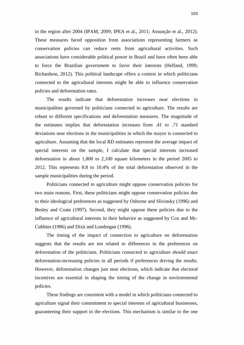
103

in the region after 2004 (IPAM, 2009; IPEA et al., 2011; Assunção et al., 2012).

These measures faced opposition from associations representing farmers as

conservation policies can reduce rents from agricultural activities. Such

associations have considerable political power in Brazil and have often been able

to force the Brazilian government to favor their interests (Helfand, 1999;

Richardson, 2012). This political landscape offers a context in which politicians

connected to the agricultural interests might be able to influence conservation

policies and deforestation rates.

The results indicate that deforestation increases near elections in

municipalities governed by politicians connected to agriculture. The results are

robust to different specifications and deforestation measures. The magnitude of

the estimates implies that deforestation increases from .41 to .71 standard

deviations near elections in the municipalities in which the mayor is connected to

agriculture. Assuming that the local RD estimates represent the average impact of

special interests on the sample, I calculate that special interests increased

deforestation in about 1,800 to 2,100 square kilometers in the period 2005 to

2012. This represents 8.8 to 10.4% of the total deforestation observed in the

sample municipalities during the period.

Politicians connected to agriculture might oppose conservation policies for

two main reasons. First, these politicians might oppose conservation policies due

to their ideological preferences as suggested by Osborne and Slivinsky (1996) and

Besley and Coate (1997). Second, they might oppose these policies due to the

influence of agricultural interests in their behavior as suggested by Cox and Mc-

Cubbins (1986) and Dixit and Londregan (1996).

The timing of the impact of connection to agriculture on deforestation

suggests that the results are not related to differences in the preferences on

deforestation of the politicians. Politicians connected to agriculture should enact

deforestation-increasing policies in all periods if preferences driving the results.

However, deforestation changes just near elections, which indicate that electoral

incentives are essential in shaping the timing of the change in environmental

policies.

These findings are consistent with a model in which politicians connected to

agriculture signal their commitment to special interests of agricultural businesses,

guaranteeing their support in the elections. This mechanism is similar to the one

104

discussed in Rogoff (1990).57

The results are also consistent with politicians

shifting to targeted distribution near elections to signal their commitment as

discussed in Drazen and Eslava (2010).

To further understand the evidence presented above, I test whether the

influence of politicians connected to agriculture on conservation policies in the

Brazilian Amazon is heterogeneous according to some local and political

characteristics. I start investigating whether the results are heterogeneous for

politicians with and without reelection incentives motivated by a long literature

documenting that these incentives affect politicians' behavior (Besley and Case,

1995; List and Sturm, 2006; Ferraz and Finan, 2011). The results suggest that

reelection incentives matter. Connection to agriculture influences deforestation in

the sample of politicians that can run for reelection, but not in the sample of

politicians that cannot run for another term. Indeed, point estimates are close to

zero when politicians do not face reelection incentives in all but one specification.

These findings reinforce the interpretation that electoral incentives induce

politicians connected to agriculture to change their behavior near elections.

I also test whether the impact is heterogeneous for politicians allied and not

allied to the federal government. Previous literature suggests that allied politicians

might find easier to affect the federal initiatives such as conservation policies.58

The results point out that the effects are similar regardless alignment to the federal

government. I then analyze whether competence influences the results using

schooling as a proxy for competence.59

Point estimates are larger in the sample of

better educated politicians compared to the sample of less educated politicians.

These estimates are suggestive that better politicians might be more able to

influence deforestation near elections. However, it is important to note that the

differences in point estimates are not large.

An important issue is which policies local officials use to influence

deforestation. That is a difficult question as several policies that can affect

57

The literature on electoral cycles indicates that signaling can induce politicians to behave

different close to elections and far from it. See Persson and Tabellini (2002) for a discussion of

such models. 58

Previous papers have identified that political connection to the federal government matters

for government transfers (Brollo and Nannicini, 2012) and access to credit (Leão et al, 2013). 59

Previous literature discusses the role of the competence of the politicians to public policies.

See Besley (2007) for a theoretical discussion of political selection and Ferraz and Finan (2009),

Besley et al. (2011) and Martinez-Bravo (2014) for empirical evidence on some of its

determinants.

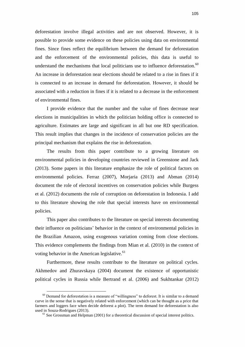
105

deforestation involve illegal activities and are not observed. However, it is

possible to provide some evidence on these policies using data on environmental

fines. Since fines reflect the equilibrium between the demand for deforestation

and the enforcement of the environmental policies, this data is useful to

understand the mechanisms that local politicians use to influence deforestation.60

An increase in deforestation near elections should be related to a rise in fines if it

is connected to an increase in demand for deforestation. However, it should be

associated with a reduction in fines if it is related to a decrease in the enforcement

of environmental fines.

I provide evidence that the number and the value of fines decrease near

elections in municipalities in which the politician holding office is connected to

agriculture. Estimates are large and significant in all but one RD specification.

This result implies that changes in the incidence of conservation policies are the

principal mechanism that explains the rise in deforestation.

The results from this paper contribute to a growing literature on

environmental policies in developing countries reviewed in Greenstone and Jack

(2013). Some papers in this literature emphasize the role of political factors on

environmental policies. Ferraz (2007), Morjaria (2013) and Abman (2014)

document the role of electoral incentives on conservation policies while Burgess

et al. (2012) documents the role of corruption on deforestation in Indonesia. I add

to this literature showing the role that special interests have on environmental

policies.

This paper also contributes to the literature on special interests documenting

their influence on politicians’ behavior in the context of environmental policies in

the Brazilian Amazon, using exogenous variation coming from close elections.

This evidence complements the findings from Mian et al. (2010) in the context of

voting behavior in the American legislative.61

Furthermore, these results contribute to the literature on political cycles.

Akhmedov and Zhuravskaya (2004) document the existence of opportunistic

political cycles in Russia while Bertrand et al. (2006) and Sukhtankar (2012)

60

Demand for deforestation is a measure of “willingness” to deforest. It is similar to a demand

curve in the sense that is negatively related with enforcement (which can be thought as a price that

farmers and loggers face when decide deforest a plot). The term demand for deforestation is also

used in Souza-Rodrigues (2013). 61

See Grossman and Helpman (2001) for a theoretical discussion of special interest politics.

106

document the existence of political cycles in the behavior of firms connected to

politicians both in France and India. I add to this literature providing evidence that

political connections change the behavior of politicians near elections.

The remaining of the paper is organized as follows. Section 2 provides

background information on deforestation and politics in the Brazilian Amazon.

Section 3 describes the data used in the estimated. Section 4 outlines the RD

design implemented in the empirical section. It also conducts some robustness

tests to validate the empirical strategy. Section 5 presents the effects of the

mayor's connection to agricultural interests on deforestation. Section 6 discusses

mechanisms. Section 7 concludes.

3.2. Institutional Background

3.2.1. Rural Politics in Brazil

Farmers constitute an important interest group in Brazil. There are well-

organized associations and unions that represent the interests of farmers both at

the local and national levels. Leaders of these organizations are often elected

politicians. For instance, the president of the leading farmers’ organization – the

Brazilian Confederation of Agriculture – is a senator. The associations

representing farmers also have ties with several other politicians across the

country. A total of 11 senators (13.5% of the total) and 191 (37.2% of the total)

federal deputies are official members of the Agricultural Caucus in the Brazilian

Congress.62

Support from legislators connected to agriculture is often essential for the

approval of most bills. The Brazilian federal government often makes concessions

to attract representatives connected to agriculture to the government coalition. In

exchange of support to the government coalition, the legislators representing

agricultural interests obtain “club public goods” and appoint members of their

caucus to important offices in the Ministry of Agriculture (Piedra, 2013). The

importance of the agricultural interests is so high that a recent issue of the

Brazilian magazine Piauí quotes the coordinator of a presidential campaign

62

Information retrieved from www.camara.gov.br in June 30, 2014.

107

stating that: “… in 30 years doing political campaigns I have never seen someone

be elected without the support [from agribusiness]”.63

Brazilian farmers became more organized during the re-democratization

period in the 1980s (Helfand, 1999). Farmers feared progressive political forces

that proposed agrarian reform and organized a powerful interest group in

Congress to fight attempts to redistribute land (Richardson, 2012). Organizations

and politicians connected to agriculture were successful in curbing land reform in

the 1990s. These organizations and politicians were also able to secure farmers

preferential access to credit and favorable tax treatment once the land reform issue

was settled (Piedra, 2013).

Land use issues in the Brazilian Amazon became more important in the

agenda of rural politics in during the past decade (Richardson, 2012). Expansion

of logging, cattle ranching and agricultural cultivation in the Brazilian Amazon

involves substantial land clearing. That created a tension between interests of the

agricultural sector in the region and environmental legislation. This tension

increased as innovative policies to fight deforestation were implemented in the

last decade. Organizations and politicians connected to agriculture have opposed

these innovations. Farmers and their representatives have proposed reforms in the

legislation to make land use policies in the Brazilian Amazon less stringent.64

Such political scenario suggests that politicians connected to agriculture will

oppose conservation policies in Brazil in order to maintain support from the

powerful organizations representing farmers and agricultural elites (Cisneros et

al., 2013). In particular, mayors connected to agricultural interests can attempt to

curb conservation policies and induce activities that lead to more deforestation.

The mechanism described above can be of particular importance during

electoral periods. Anecdotal evidence suggests that deforestation increases near

elections. The newspaper Folha de São Paulo wrote in a recent article on the rise

of deforestation in the months preceding the previous election that “(…) electoral

years usually have increases in deforestation, supposedly due to lower

63

Piauí, July 2014, p. 22. 64

The Economist (2012) reports the tension between farmers’ interests and environmental

conservation in the debates around the reform of the Brazilian Forest Code.

108

fiscalization (…)”.65

Hence, it is important to investigate the effect of agricultural

interests on deforestation in different moments of the electoral cycle.

3.2.2. Deforestation in the Brazilian Amazon

Deforestation in the Brazilian Amazon became an important public policy

issue over the past decades. More than 750,000 square kilometers of forest area

were deforested over the past four decades in the region. The main drivers of

deforestation were the construction of roads and the expansion of population in

the area after 1970 (Pfaff, 1999; Pfaff et al., 2007). These factors induced logging

and cattle ranching activities that involve substantial land clearing. Poor

institutions reinforced the incentives for unsustainable land use as clearing often

helps to secure land rights in the Brazilian Amazon (Alston et al., 2000).

Increased deforestation led to a major reorganization in conservation

policies in the Brazilian Amazon. In 2004, the federal government created Action

Plan for the Prevention and Control of Deforestation in the Legal Amazon

(PPCDAM). This initiative integrated actions across different agencies and

introduced innovative tools for monitoring deforestation and curbing deforestation

(IPAM, 2009).

Policies implemented under the PPCDAM can be divided into two phases.

At the beginning, the government focused on the establishment of protected areas,

in the improvement of deforestation monitoring using satellite data and in the

expansion of the number of operations from the environmental protection agency

(IBAMA). These initiatives resulted in the establishment of over 180,000 square

kilometers of protected areas and the creation of a real-time deforestation

monitoring system using satellite data (DETER).

Better data and investments in staffing and training the environmental

protection agency led to a sharp increase in the number of fines in the period

(Hargrave and Kis-Katos, 2013). However, environmental fines are often not paid.

Its coercive effect on deforestation comes from consequences from the operations

that lead to fines such as the embargo of the land and the expropriation of the

deforested timber (Assunção et al., 2013a).

65

“Desmatamento na Amazônia dispara em agosto e setembro”, Folha de São Paulo,

November 11, 2014.

109

The government expanded the set of polices implemented under the

PPCDAM after 2008. First, it conditioned access to credit for agricultural

activities in the Brazilian Amazon to compliance with the environmental

legislation (Assunção et al., 2013b). Second, it created a blacklist of high

deforestation municipalities in which conservation efforts were concentrated.

Politicians, credit agencies and agricultural traders operating in these

municipalities also face pressure from the federal government to induce changes

in practices related to unsustainable land use that result in forest clearing.

Blacklisted municipalities face higher presence of the environmental protection

agency (IBAMA) and other government agencies involved with land use.

The combination of these initiatives led to a reduction in deforestation in the

Brazilian Amazon over the last decade (IPEA et al., 2011; Assunção et al., 2012).

This decline highlights the importance of the federal government in fighting

deforestation in the region. However, there is still substantial variation in

deforestation rates across municipalities in the Brazilian Amazon. Local policies

and economic characteristics continue to be important determinants of the

deforestation rates.

3.2.3. Role of Mayors on Environmental Policies

Municipalities are the lower administrative division in Brazil. Municipal

governments are managed by an elected mayor (Prefeito) and an elected city

council (Câmara dos Vereadores). Municipal elections are held at the same time

in all municipalities and happen in October of the election year. The elected

officers start a four years term in January of the following year.

Local councilors are elected using a proportional system. Mayors are elected

for a four years term using a plurality rule in all municipalities with less than

200,000 eligible voters and a majority rule in municipalities with more than

200,000 eligible voters.66

Mayors can run for reelection once while local

councilors can run for reelection indefinitely.

Mayors are responsible for the executive branch while councilors are

responsible for the legislative branch of the municipal government. The executive

branch concentrates the most relevant choices concerning public policies. It is the

66

The empirical analysis focuses on municipalities with less than 200,000 voters.

110

executive branch who establishes partnerships with the federal and state

governments, proposes a budget, and implements public policies (Brollo et al.,

2013).

Municipal governments are responsible for a substantial share of the

provision of public goods and services in areas such as education, healthcare, and

infrastructure. Local governments also manage the distribution of conditional cash

transfers as well as most schools and health facilities.67

A large share of the

expenditures on these public goods is financed from transfers from the federal

government.68

The municipal governments also have responsibilities regarding

environmental policies often acting in cooperation with higher levels of

government (Leme, 2011). These governments can influence the effectiveness of

conservation policies and affect deforestation enacting policies that change the

demand for deforestation. For instance, land clearing is often associated with

activities such as illegal land sales, land grabbing, and logging. These activities

require consent from local authorities to take place and therefore municipal

governments are crucial in determining the rate that these events take place

(Fearnside, 2001; Cisneros et al., 2013).

Local authorities can also affect deforestation changing the incidence of

federal policies through lobbying, bribes, and threats. Lobbying with federal

authorities can influence the presence of the environmental protection agency or

the supply of rural credit in the municipality. Bribes to officers from the

environmental protection and credit agencies can have a similar effect. In

addition, local authorities can threaten and even use violence against bureaucrats

who operate in their municipalities. These actions might changes the incidence of

federal policies and affect deforestation.69

However, it is important to note that enacting policies to induce higher

deforestation can have significant costs to local authorities. These actions often

67

The Brazilian Constitution from 1988 led to a large restructuring in the provision of public

goods in Brazil with municipalities becoming more important in the provision of education,

healthcare, sanitation, habitation etc. See Arretche (1999) for an analysis of the decentralization

process following the 1988 constitution. 68

See Afonso and Araújo (2000) for a discussion of the role of transfers and the imbalances it

creates. 69

See Assunção et al. (2013a) for evidence on the relationship between presence of the

environmental protection agency and deforestation and Assunção et al. (2013b) for evidence on

the relationship between credit and deforestation.

111

involve illegal activities and authorities can be punished if these activities are

disclosed.70

These actions can also trigger punishments from the federal

government, which can reduce federal transfers municipal governments receive or

loans that local businesses obtain from public banks.71

These punishments can

influence public goods provision and economic performance given the importance

both of federal transfers for government financing and of access to credit from

public banks for firm financing in the Brazilian municipalities.

3.3.Data and Sample Selection

3.3.1. Electoral Data

The empirical design relies on a measure of connection to agricultural

interests. This measure indicates whether a candidate for mayor is connected to

agriculture and is the treatment variable in the empirical analysis. I construct this

measure using data on characteristics of the candidates who ran for mayor in

Brazil. I use data from the municipal elections of 2004 and 2008. The data is

available from the Tribunal Superior Eleitoral (TSE) and provides information on

characteristics such as gender, age, education and occupation for all candidates.

I construct the political connection measure using data on occupations. I

define a candidate as “connected to agriculture” if the candidate reports having an

agricultural occupation as the principal occupation. These candidates are called

“farmers” in the remaining of the paper. I code agronomists, land surveyors,

farmers, cattle ranchers and farm workers as “farmers”. There were 4,749

candidates running for mayor in the municipalities of the Brazilian Amazon in the

municipal elections of 2004 and 2008. A total of 743 candidates (15.67 percent)

were considered connected to agriculture according to this definition.

The political connection measure defined above underestimates the number

of politicians connected to agriculture. There might be many candidates connected

to agriculture who report working in “other occupations”. Also, some candidates

whose original occupation was agricultural might answer working as politicians

despite still having interests in agriculture. Other candidates, whose occupation is

70

Punishment can be either judicial or electoral. Ferraz and Finan (2008) present evidence that

disclosure of corrupt activities reduces electoral performance. 71

The blacklisting initiative described earlier is an example of punishment from the federal

government on municipalities with high deforestation rates.

112

not agricultural, can receive political support from lobbies and interest groups

connected to agriculture.

This measurement error in political connection will bias downwards the

estimated impact of connection to agriculture on deforestation to the extent that

the measurement error is not correlated with deforestation rates. The estimates

presented in the following sections are a lower bound of the actual effect of

connection to agriculture on deforestation under this scenario. However,

alternative assumptions about the relationship between measurement error and

deforestation can alter the direction of the bias. If the measurement error is larger

in municipalities with higher deforestation, than the estimates presented in the

following sections can be biased upwards and represent an upper bound of the

relationship between connection to agricultural interests and deforestation.72

Other variables drawn from the TSE are also used in the empirical analysis.

I use this dataset to construct the following variables: margin of victory, total

turnout, number of candidates, vote concentration, age, reelection incentives,

alignment with the federal government, and schooling. The margin of victory is

used to implement the Regression Discontinuity (RD) design. Total turnout, vote

concentration, number of candidates and age are used in specification tests that

investigate whether there are discontinuities in pre-determined outcomes.

Reelection incentives, alignment with the federal government and schooling are

used to test whether the effects of the mayor's connection to agricultural interests

are heterogeneous.

3.3.2. Data on Deforestation

The main outcome used in the empirical design is deforestation. The data of

deforestation is built using satellite images processed by the Project for

Monitoring Deforestation in the Brazilian Amazon (PRODES/INPE). Technicians

working for PRODES/INPE treat the raw satellite images to identify deforested

72

An alternative measure of connection to agriculture could be constructed using data from

assets that the candidates report to own. This measure is used in Richardson (2012) who

investigates the impact of land conflict on entry of politicians connected to agriculture. The author

codes a candidate as connected to agriculture if the candidate reports to own land. However, data

to construct it is unavailable for the election of 2004 and would limit sample size.

113

areas. The areas are then aggregated to produce deforestation estimates for all

municipalities in the Brazilian Amazon.73

The PRODES project was established in 1999 and produces deforestation

for the Brazilian Amazon estimates since then. However, the available data from

the period 1999 to 2001 and from period 2002 to 2013 is not comparable due to

methodological changes. I use data from 2005 to 2012 to cover the period that

mayors elected in 2004 and 2008 were in office. Deforestation is defined as the

annual deforestation increment, which is the area of forest cleared over the past

twelve months. Deforestation in year 𝑡 is the area in square kilometers cleared

from August 1 of year 𝑡 − 1 to July 31 of year 𝑡. The timing is an important

feature of the data on deforestation as it creates a mismatch data on political

connections and deforestation. I return to this issue in the results section.

I smooth differences in deforestation across municipalities using a

normalized deforestation measure proposed in Assunção et al. (2012). Let 𝐼𝑚𝑡 be

the number of square kilometers deforested in municipality 𝑚 and period 𝑡. Also

let 𝐼𝑚 be the average deforestation in 𝑚 and 𝑠𝑑(𝐼𝑚) be the standard deviation of

deforestation in 𝑚 over the sample period. I define the normalized deforestation

rate 𝐷𝑚𝑡 as:

𝐷𝑚𝑡 =𝐼𝑚𝑡 − 𝐼𝑚

𝑠𝑑(𝐼𝑚𝑡)

The normalized deforestation rate 𝐷𝑚𝑡 indicates whether deforestation in

municipality 𝑚 in year 𝑡 was high or low compared to the average deforestation in

𝑚 observed in the sample years. This is the preferred measure of deforestation

used throughout the paper. The advantage of the normalized deforestation rate is

that it ensures that differences in deforestation observed across municipalities are

related to differences in total area or differences in historical land use.

I also use a couple of other measures used in the previous literature in the

estimates to check whether the results are driven by the definition of deforestation.

First, I follow Morjaria (2013) and define the deforestation rate as the area of

forest cleared over the past twelve months.74

Second, I follow Pfaff (1999) and

Pfaff et al. (2007) and define the deforestation rate as the ratio between the area of

73

Detailed information on the PRODES/INPE and on the construction of the data can be

found in PRODES (2013). 74

Burgess et al. (2012) also uses a similar measure. The main difference is that the

deforestation data he uses is discrete.

114

forest cleared over the past twelve months and the original forest area. Note that

the first alternative measure does not smooth out variation in deforestation across

municipalities related to differences in total area or historical land use. The second

alternative measure smooths out variation in deforestation related to differences in

total area, but not to differences in historical land use.

Other data from PRODES/INPE are also used in specification tests. I use the

dataset to construct four variables: total area, forest area, unobserved areas, and

cloud coverage. These variables are used to test whether there are discontinuities

in pre-determined outcomes.

3.3.3.Environmental Fines

I use annual data on environmental fines from the Brazilian Environmental

Protection Agency (IBAMA) to test whether connection to agriculture affects both

the number and the value of environmental fines in a given year. This data is the

same used in Assunção et al. (2013a). This data is not available for the year 2012.

That limits the analysis to the electoral cycle from 2005 to 2008. I return to this

issue in the discussion of the results.

3.3.4.Sample Selection

Data on deforestation is available for all 774 municipalities monitored by

PRODES/INPE. Municipalities with no deforestation in all sample years and

municipalities in the top 1% of the deforestation distribution in each sample year

are excluded from the sample. I drop the first group of municipalities to ensure

that the analysis is focused in municipalities in which deforestation is a salient

issue. I exclude the second group of municipalities to ensure that outliers are not

driving the results. The main estimates are robust to including both groups of

municipalities.

The estimates are based on a RD design that compares municipalities in

which a candidate connected to agriculture won the election against a candidate

not connected to agriculture and municipalities in which a candidate connected to

agriculture lost the election to a candidate not connected to agriculture. Therefore,

I focus on municipalities in which either the winner or the runner-up is connected

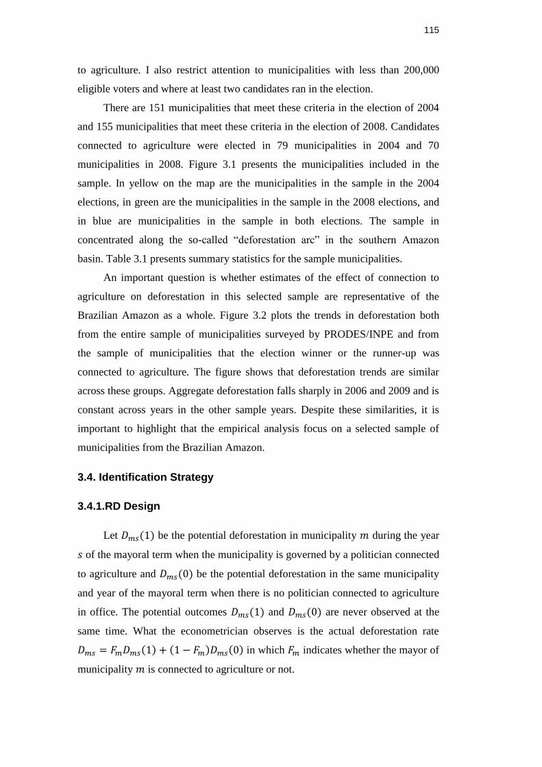
115

to agriculture. I also restrict attention to municipalities with less than 200,000

eligible voters and where at least two candidates ran in the election.

There are 151 municipalities that meet these criteria in the election of 2004

and 155 municipalities that meet these criteria in the election of 2008. Candidates

connected to agriculture were elected in 79 municipalities in 2004 and 70

municipalities in 2008. Figure 3.1 presents the municipalities included in the

sample. In yellow on the map are the municipalities in the sample in the 2004

elections, in green are the municipalities in the sample in the 2008 elections, and

in blue are municipalities in the sample in both elections. The sample in

concentrated along the so-called “deforestation arc” in the southern Amazon

basin. Table 3.1 presents summary statistics for the sample municipalities.

An important question is whether estimates of the effect of connection to

agriculture on deforestation in this selected sample are representative of the

Brazilian Amazon as a whole. Figure 3.2 plots the trends in deforestation both

from the entire sample of municipalities surveyed by PRODES/INPE and from

the sample of municipalities that the election winner or the runner-up was

connected to agriculture. The figure shows that deforestation trends are similar

across these groups. Aggregate deforestation falls sharply in 2006 and 2009 and is

constant across years in the other sample years. Despite these similarities, it is

important to highlight that the empirical analysis focus on a selected sample of

municipalities from the Brazilian Amazon.

3.4. Identification Strategy

3.4.1.RD Design

Let 𝐷𝑚𝑠(1) be the potential deforestation in municipality 𝑚 during the year

𝑠 of the mayoral term when the municipality is governed by a politician connected

to agriculture and 𝐷𝑚𝑠(0) be the potential deforestation in the same municipality

and year of the mayoral term when there is no politician connected to agriculture

in office. The potential outcomes 𝐷𝑚𝑠(1) and 𝐷𝑚𝑠(0) are never observed at the

same time. What the econometrician observes is the actual deforestation rate

𝐷𝑚𝑠 = 𝐹𝑚𝐷𝑚𝑠(1) + (1 − 𝐹𝑚)𝐷𝑚𝑠(0) in which 𝐹𝑚 indicates whether the mayor of

municipality 𝑚 is connected to agriculture or not.

116

I am interested in estimating the causal effect of connection to agriculture on

deforestation. Consider a simple estimator of the causal effect of connection to

agriculture on deforestation in term year 𝑠 given by:

𝐸[𝐷𝑚𝑠|𝐹𝑚 = 1] − 𝐸[𝐷𝑚𝑠|𝐹𝑚 = 0]

This estimator is a simple comparison of the average deforestation in

municipalities governed by politicians connected to agriculture with the average

deforestation in municipalities not governed by politicians connected to

agriculture. It is well known that this estimator will be biased unless political

connected is assigned randomly and there is no selection bias.75

However, elections are not random and municipalities in which mayors are

connected to agriculture are probably quite different from the other municipalities.

It is possible that municipalities in which the political strength of politicians

connected to agriculture is higher are municipalities with differences in

agricultural potential, land use, access to markets etc. All these factors influence

deforestation according to the literature (Pfaff, 1999; Pfaff et al., 2007; Souza-

Rodrigues, 2013).

I use a RD design based on close elections to eliminate the selection bias

and estimate the causal effect of connection to agriculture on deforestation. The

RD design explores the fact that the winner of a close election is random. Hence,

there will be no selection bias in close elections and it is possible to estimate the

causal effect of connection to agriculture on deforestation in these elections.

Let 𝑀𝑉 be the margin of victory of the elected candidate. The causal effect

of connection to agriculture on deforestation in close elections is:

𝐸[𝐷𝑚𝑠(1) − 𝐷𝑚𝑠(0)|𝑀𝑉 = 0] = lim𝜀↓0

𝐸[𝐷𝑚𝑠|𝑀𝑉 = 휀] − lim𝜀↑0

𝐸[𝐷𝑚𝑠|𝑀𝑉 = 휀] (3.1)

The estimator above is consistent whenever the distribution of the potential

outcomes conditional on 𝑀𝑉 is continuous at the threshold 𝑀𝑉 = 0 (Imbens and

Lemieux, 2008). The quantities in the right-hand side of equation (3.1)

(lim𝜀↓0 𝐸[𝐷𝑚𝑠|𝑀𝑉 = 휀] and lim𝜀↑0 𝐸[𝐷𝑚𝑠|𝑀𝑉 = 휀]) are observed in the data and

therefore the estimator above can be computed using observational data.

There are several alternative methods to estimate equation (3.1). One

alternative is to use local linear regression and estimate the following equation for

municipalities with close elections in which 𝑀𝑉 ∈ [−𝑏, 𝑏]:

75

See Angrist and Pischke (2008) for a discussion of the selection bias in a similar

framework.

117

𝐷𝑚𝑠 = 𝛼 + 𝛽𝑠𝐹𝑚 + 𝛾𝑠𝑀𝑉𝑚 + 𝜌𝑠(𝐹𝑚x𝑀𝑉𝑚) + 𝑢𝑚𝑠 (3.2)

The coefficient of interest in the equation above is 𝛽𝑠 and it represents the

causal effect of connection to agriculture on deforestation during the year 𝑠 of the

mayoral term at 𝑀𝑉 = 0. 𝛽𝑠 > 0 indicates that politicians connected to

agriculture increase the deforestation rate in year 𝑠 of the term.

The local linear estimator presented above has a simple intuition. It fits a

line below and above the threshold and identifies the impact as the difference in

intercept between these lines at 𝑀𝑉 = 0. Selection of 𝑏 can be either ad hoc or

use the optimal bandwidth selection method from Imbens and Kalyanaraman

(2012). One should note that a smaller bandwidth reduces the bias at cost of

efficiency.

An alternative method is to estimate a polynomial spline of order 𝑝 using all

observations:

𝐷𝑚𝑠 = 𝛼 + 𝛽𝑠𝐹𝑚 + ∑ 𝛾𝜈𝑠𝑀𝑉𝑚𝜈

𝑝

𝜈=1

+ ∑ 𝜌𝜈𝑠(𝐹𝑚x𝑀𝑉𝑚)𝜈

𝑝

𝜈=1

+ 𝑢𝑚𝑠 (3.3)

The coefficient of interest in the equation above is 𝛽𝑠 which again represents

the causal effect of connection to agriculture on deforestation at 𝑀𝑉 = 0. The

polynomial spline estimator fits a polynomial below and above the threshold and

identifies the impact as the difference in intercept between these polynomials at

𝑀𝑉 = 0.

I pool together two electoral terms to increase power of the estimates.

Therefore, the main estimates include year dummies as controls in order to

increase the precision of the estimates. Year 1 of the mayoral term represents

deforestation outcomes in 2005 and 2009. Year 2 represents deforestation

outcomes in 2006 and 2010. Year 3 represents deforestation outcomes in 2007

and 2011. Year 4 represents deforestation outcomes in 2008 and 2012.

I estimate 𝛽𝑠 for different moments of the mayoral term in order to

understand whether mayors connected to agriculture influence deforestation

changes across the electoral cycle. That helps to understand whether connection to

agriculture affects deforestation due to preferences of the politician or the interest

group. Equal 𝛽𝑠 across periods indicates that the increase in deforestation is not

related to politics and that preferences of the politician are driving the result.

However, a higher 𝛽𝑠 close to elections indicates that politicians connected to

118

agriculture cater to the preferences of the interest group either when the costs of

doing so are not observed or when salience of policies favoring deforestation is

higher.

The main pitfall from the RD design is that it estimates a local treatment

effect. This effect can be quite different from the average effect in the sample. In

the studied context, the RD estimates represent the treatment effect of connection

of the politician in office to agricultural interests in the group of municipalities

where elections were competitive. This effect can be different from the effect of

connection to agriculture in municipalities in which competition is not so high.

Therefore, I also report results of OLS and Fixed Effects specifications to

compare the results from RD estimates with from other estimation methods.76

3.4.2. Specification Tests

The identification assumption of the RD design is that candidates connected

to agriculture are not able to sort above or below the threshold. This assumption

guarantees that close elections are random and validates the design. Existing

research have shown that close elections are not random in some contexts.

Therefore, it is important to consider whether there is evidence of sorting before

presenting the main estimates.

It is important to highlight that the identification assumption is not testable.

However, it is possible to obtain indirect evidence supporting it using

specification tests designed in the literature. These tests explore some testable

implications of the identification assumption. The first implication concerns the

smoothness of the distribution of the treatment variable at the threshold. Sorting

around the threshold would make candidates to concentrate at one side of it. This

implies that sorting would make the distribution of connection to agriculture to be

discontinuous at the threshold. Sorting can be tested using the manipulation test

proposed by McCrary (2008).

The results from this test are presented in Figure 3.3. There is no evidence

that the distribution of connection to agriculture jumps at the threshold (the point

estimate is -0.09 and the standard error is 0.20). The evidence from the McCrary

test is consistent with the identification assumption.

76

It is important to note that coefficients estimated using other estimation methods might not

be consistent.

119

Further evidence favoring the identification assumption can be obtained

testing whether predetermined observable characteristics jump at the threshold.

Pre-determined variables should not jump at the threshold since close elections are

random and connection to agricultural interests must not be correlated with

municipal characteristics at 𝑀𝑉 = 0. I test this implication for two different sets

of covariates. The first is a group of political outcomes. These outcomes are

turnout, number of candidates, vote concentration and age. The second is a group

of land use variables. These outcomes are total area, total forest area, area not

observed and cloud coverage.

The results from these specification tests are presented in Table 3.2.

Columns 1 to 4 present the results for electoral outcomes. Columns 5 to 8 present

the results for land use variables. Each panel reports estimates obtained using a

different estimation technique. The estimates indicate that pre-determined

outcomes do not change at the threshold. No estimated coefficient is significant at

the 5% level or the 10% level.

Figure 3.4 presents a graphical representation of the results for the electoral

variables using a cubic polynomial splice estimated for the selected bandwidth at

𝑀𝑉 ∈ [−40, 40]. Figure 3.5 presents the same graphical representation for the

land use outcomes. Both figures reinforce the interpretation that predetermined

outcomes do not change at the threshold. Pre-determined outcomes seem to be

similar in both sides of the threshold. These results lend support to the assumption

that the distribution of the potential outcomes conditional on 𝑀𝑉 is continuous at

the threshold.

3.5. Results

3.5.1. Farmers and Deforestation: OLS and FE

I start documenting the correlation between connection to agriculture and

deforestation in the sample municipalities. I regress the normalized deforestation

rate on interactions between dummies indicating whether the mayor is connected

to agriculture (Farmer) and the year of the mayoral term (Year) and a set of

controls. I use four different specifications. The first specification includes only

year dummies as controls. The second specification additionally includes the

mayor party and interactions between the original forest cover and time dummies

120

as controls. The third specification further includes state fixed effects as controls.

The fourth specification replaces state fixed effects by municipal fixed effects and

uses only variation coming from municipalities whose mayor connections

changed in the period. The results are presented in Figure 3.6. Each panel reports

the estimates from one specification. The dots correspond to the coefficients of

interest and the dashed lines to 90% confidence intervals.

Panel A reports estimates using no controls. The results indicate that

municipalities where a farmer is in office have a higher deforestation rate in the

second and the fourth years of the mayoral term. Both are electoral years, with

elections for the State and Federal Congresses and Governments happening in the

second year and elections for Municipal Governments in the fourth year. The

correlation is significant at the 10% level for the second year, but not for the

fourth year.

Panels B includes additional covariates in the estimation. The results are

similar to the presented in the previous panel. Both the magnitude and the

standard errors of the coefficients remains similar. Panel C includes state fixed

effects in the estimation. Again, the results are unaltered with the change in the

specification.

Panel D replaces the state fixed effects for municipal fixed effects. Point

estimates become larger and significant at the 10% level for both the second and

the fourth year of the mayoral term. Point estimates remain close to zero and

insignificant at the usual statistical levels in the first and third term year. The

magnitude of the coefficients implies that municipalities with farmers in office

have about .3 standard deviations higher deforestation in electoral periods.77

These results suggest that politicians connected to agriculture change their

behavior near elections to benefit the interests of the farming sector.

However, the presence of politicians connected to agriculture is not random

and these results might be biased. For instance, suppose that the likelihood of

having a politician connected to agriculture is correlated with the predominance of

cattle grazing. In addition, suppose that the federal government expands

agricultural credit during electoral periods and that more credit increases

deforestation in areas in municipalities in which cattle grazing is predominant as

77

Note that the normalized deforestation has mean zero and standard deviation one so the

interpretation is direct from the estimated coefficients.

121

documented in Assunção et al. (2013b). Under these assumptions, the estimates

from Figure 3.6 overestimate the impact of connection to agriculture on

deforestation if the correlation between the presence of farmers in office and cattle

grazing is positive and underestimate this effect if the correlation is negative.

The RD design deals with the omitted variable bias that might affect the

estimates using the specifications presented in Figure 3.6. Nevertheless, it is worth

stressing that the RD method estimates the average impact of connection to

agriculture on deforestation for a group of municipalities for which elections are

competitive. This impact can be different from the average impact in the full

sample of municipalities.78

3.5.2.Farmers and Deforestation: RD Estimates

Table 3.3 presents the main estimates obtained using the Regression

Discontinuity (RD) design described in the previous section. Columns 1 to 4

report estimates in which the dependent variable is normalized deforestation.

Columns 5 to 8 report estimates in which the dependent variable is deforestation

in square kilometers. Columns 9 to 12 report estimates in which the deforestation

measure is the deforestation as a share of the total forest area.

Panel A estimates equation (3.2) using the optimal bandwidth estimator

proposed by Imbens and Kalyanaraman (2012). This method uses an optimality

rule to select the observations included in the estimation. Panel B estimates

equation (3.2) for electoral races in which the margin of victory is smaller than

10% (𝑀𝑉 = [−10, 10]). Panel C estimates equation (3.3) for a cubic polynomial

(𝑝 = 3) using electoral races in which the margin of victory is smaller than 40%

(𝑀𝑉 = [−40, 40]).

The results from columns 4, 8 and 12 indicate that deforestation is higher in

municipalities governed by farmers in the fourth year of the mayoral term. The

results are robust to different measures of deforestation and estimation methods

and are significant either at the 5% or the 10% level. The coefficients not

significant at the 5% level have p-values close to 5%.79

78

It is impossible to determine whether differences between effects of connection to

agriculture on deforestation estimated using OLS and FE and estimated using RD reflect bias in

OLS and FE or different impacts in competitive elections and in all municipalities. 79

Four of the twelve estimates of the effect of connection to agriculture on deforestation close

to elections are not significant at the 5% level. However, these coefficients have p-values close to

122

The results from the other columns suggest that there are no differences in

deforestation across municipalities governed by farmers in the other periods. Point

estimates are often close to zero and are not significant at the usual statistical

levels for almost all deforestation measures and estimation methods. The

exception is the coefficient from column 5 in Panel A that is significant at the

10% level.

It is important to highlight that the impact of connection to agriculture on

deforestation is not driven by changes in deforestation after elections (that are

held in October). That happens because the deforestation rate in a given year

represents the total deforestation between August 1 of the previous year and July

31 of the given year. This feature of the data ensures that the causal impact of

connection to agriculture on deforestation estimated in columns 4, 8 and 12 is due

to policies implemented before the elections took place.

The magnitude of the estimated impact of connection to agriculture on

deforestation in election years is substantial. Estimates in column 4 suggest that

having a politician connected to agriculture in office increases deforestation in .64

to .71 standard deviations of the normalized deforestation measure. Estimates in

column 8 indicate that having a politician connected to agriculture in office

increases deforestation in .41 to .49 standard deviations of deforestation in square

kilometers. In addition, estimates in column 12 provide evidence that having a

politician connected to agriculture in office increases deforestation in .47 to .58

standard deviations of deforestation as a share of the forest area.

The findings reported above are different from the results from Figure 3.6 in

some important aspects. RD estimates do not provide evidence that deforestation

increases in municipalities with farmers in office near presidential, gubernatorial

and congressional elections as suggested in Figure 3.6. RD estimates also suggest

that the impact of farmers on deforestation near municipal elections is higher than

suggested in Figure 3.6.

Figures 3.7 and 3.8 present a graphical representation of the results. Figure

3.7 plots the estimates from Panel B, while Figure 3.8 plots the estimates from

Panel C. Each graph plots the estimates for a different year of the term. Both

0.05. The coefficient estimated in Panel B, column 8 has p-value 0.068; the coefficient estimated

in Panel A, column 12 has p-value 0.057; the coefficient estimated in Panel B, column 12 has p-

value 0.054; and the coefficient estimated in Panel C, column 12 has p-value 0.059.

123

figures use the normalized deforestation as the deforestation outcome. The figures

provide evidence that the effect of farmers on deforestation close to elections is

related to increases in deforestation in municipalities governed by farmers (as

opposed to declines in deforestation in these municipalities).

The concentration of the impact of connection to agricultural interests on

deforestation near elections implies that preferences of the politician are not

explaining the relationship between these variables. If preferences of the politician

were the mechanism, deforestation in municipalities in which a farmer is in office

should be higher in all periods. The results are consistent with a model in which

politicians take costly actions near elections to signal their commitment with

particular interest groups and attract their electoral support.80

A simple mechanism can explain signaling during electoral periods and not

off electoral periods. Suppose that some actions (such as lobbying to reduce the

incidence of conservation policies or bribing officials to tolerate deforestation)

have benefits observable in the short run, but costs that are observable only in the

long run. This is plausible in the context studied as it takes time to the authorities

to punish municipalities with high deforestation rates (either through legal action

or through reduction of transfers and investments in these municipalities).

Suppose also that there are uncertainties on the commitment of incumbent

politicians with an interest group. This implies that it is rational for its members to

maintain the support to the incumbent politician based on the benefits received

during his term of office. In this context, it is optimal for office-seeking

politicians to enact policies that benefit the interest groups connected to them near

elections and not far from them. The existence of behavioral biases that increase

the importance of policies enacted in more salient periods (such as electoral

periods) just increases these incentives.

The cost of catering to special interests appears to be substantial. Assume

that the local RD estimates represent the average impact of special interests on the

sample. In this scenario, it is possible to use the coefficients in column 8 from

Table 3.3 to calculate the impact of catering to special interests. I estimate that

catering to special interests increased deforestation in about 1,800 to 2,100 square

80

Rogoff (1990) is an example of a model in which politicians change policies near elections

to signal their competence. However, in his model politicians’ signal to the electorate while here

the results suggest that the politicians signal to interest groups.

124

kilometers in the period 2005 to 2012. This represents 8.8 to 10.4% of the total

deforestation observed in the sample municipalities during the period.

3.5.3.Heterogeneous Effects

The interpretation of the RD results put forward above implies that electoral

incentives induce politicians to enact policies that increase the deforestation rate

near elections. An additional implication of this interpretation is that politicians

with reelection incentives have higher incentives to enact policies that increase

deforestation.81

I test this implication showing that the impact of connection to

agriculture on deforestation near elections is different for politicians with and

without reelection incentives.

Table 3.4, columns 1 and 2 report the results from these estimations. Panels

A to C represent the coefficients estimated using different estimation methods

(local linear with optimal bandwidth, local linear with determined bandwidth and

cubic spline). Column 1 presents the results from the sample of politicians with

reelection incentives while column 2 presents the results from the sample of

politicians without reelection incentives. The dependent variable across all

specifications is the normalized deforestation rate.

The estimates from column 1 point out that deforestation increases near

elections in municipalities with farmers in office when the politicians have

reelection incentives. The point estimates are about ten percent higher than the

estimates obtained with the full sample and are similar across different estimation

methods. In contrast, the estimates from column 2 provide evidence that

politicians connected to agriculture do not affect deforestation near elections when

the politicians do not have reelection incentives. Point estimates are not

significant and are smaller than the point estimates from column 1 across Panels

A-C. The point estimates are also close to zero when local linear regressions are

used (Panels A and B). The results are consistent with the interpretation of the

main estimates. Politicians connected to agriculture seem to change their behavior

81

Politicians might still get rents from office when help to elect a politician from the same

political coalition. However, these rents will be lower than the rents the politician gets when she is

in office. Indeed, there is a long literature that documents the importance of reelection incentives

to the behavior of incumbent politicians. See, for example, Besley and Case (1995) for evidence

on the impact of term limits on the economic performance of the American states, List and Sturm

(2006) for evidence on the impact of term limits on environmental policies in the U.S. and Ferraz

and Finan (2011) for evidence on the impact of term limits on corruption in Brazil.

125

to benefit farming interests to increase electoral support and increase their

reelection chances.

The impact of connection to agriculture on deforestation near elections can

also be heterogeneous according to the membership of the politician in the federal

government coalition. Members of the coalition might find easier to influence

federal policies that affect deforestation (such as operations from the

environmental protection agency or supply of agricultural credit from official

banks). I test this implication estimating whether the impact of connection to

agriculture on deforestation near elections is different for politicians allied or not

with the federal government. Table 3.4, columns 3 and 4 report the results from

these estimates. Column 3 reports the impact of connection to agriculture for

allied politicians while column 4 reports the impact for non-allied politicians. The

estimation methods used across Panels A-C are local linear regression with

optimal bandwidth, local linear regression with determined bandwidth, and cubic

spline.

The results in columns 3 and 4 from Table 3.4 are inconclusive. Point

estimates in the sample of aligned and unaligned politicians are similar across all

estimation methods. Standard errors are quite large which limits the statistical

inference. There is no consistent evidence that politicians connected to agriculture

find it easier to affect deforestation when they belong to the government coalition.

It might also be the case that the effect of connection to agriculture on

deforestation is heterogeneous according to differences in educational attainment.

A growing literature indicates that educational attainment and other competence

measures can matter for political performance (Ferraz and Finan, 2009; Besley et

al., 2011; Martinez-Bravo, 2014). In the context studied, competence can help

politicians to insulate their actions from special interests or it can help them to

favor the special interests. I investigate these mechanisms testing whether the

impact of connection to agriculture on deforestation near elections is different in

samples of more and less educated politicians. Columns 5 to 6 from Table 3.4

report the results from these estimates. Again, I use three different estimation

methods (local linear with optimal bandwidth, local linear with determined

bandwidth and cubic spline) across Panels A-C. The results suggest that better

educated politicians are more able to favor the special interests and enact policies

that increase deforestation. Point estimates for politicians that completed high

126

school (column 5) are higher than for politicians that did not complete high school

(column 6). In addition, the point estimates for more educated politicians are

significant at the 10% level across the three estimation methods while the

estimates for less educated politicians are not significant.

3.6.Mechanism: Enforcement or Demand for Deforestation?

The results from the previous section indicate that mayors connected to

agriculture affect deforestation rates near elections. An important question is

which policies these politicians use to influence deforestation. For instance,

politicians might attempt to lobby, bribe or even threaten bureaucrats from

environmental agencies, official banks, and local land registries. While all these

actions might affect deforestation, most are unobserved. Therefore, it is hard to

pin down the exact policies that politicians connected to agriculture use to

influence deforestation in electoral periods.

Despite these difficulties, data on environmental fines is useful to

understand the mechanisms that local politicians use to influence deforestation.

Environmental fines have a significant coercive effect on deforestation in the

Brazilian Amazon. The existing literature indicate that more fines reduce

deforestation (Hargrave and Kis-Katos, 2013; Assunção et al., 2013a). These fines

reflect the equilibrium between the demand for deforestation and the enforcement

of environmental policies. Conditional on enforcement, both deforestation and

fines increase when the demand for deforestation rises. Conditional on the

demand for deforestation, deforestation increases and fines decrease when the

enforcement of environmental policies declines. Hence, the changes in fines

inform whether the increase in deforestation near elections observed in

municipalities with a mayor connected to agriculture is due to a rise in demand or

a decline in enforcement.

I test the effect of having a farmer in office on the number and the value of

the fines using the same identification strategy used in the previous estimates.

However, the estimation methods are different from the ones used before. On the

one hand, data on the number of fines is discrete, suggesting that a Poisson model

should be used to estimate the effect of having a farmer in office on this variable.

On the other hand, data on the value of fines per forest area is left censored,

suggesting that a Tobit model should be used to estimate the effect of having a

127

farmer in office on this variable. As discussed earlier, these data is not available

for the whole sample period limiting the estimates to data for the period 2005-

2008.

The effects of connection to agriculture on environmental fines are reported

in Table 3.5. Column 1 reports the bivariate relationship between fines and

connection to agriculture. Column 2 controls for the margin of victory using a

linear term. Column 3 controls for the margin of victory using a quadratic term.

Column 4 controls for the margin of victory using a cubic term. Columns 5, 6 and

7 include splines to allow the polynomials to be different above and below the

threshold.

Panel A reports the estimates for the number of fines. Column 1 suggests

that there are no differences in the number of fines across municipalities governed

by farmers or not. The RD estimates from the other columns indicate that the

number of fines falls near elections in municipalities with mayors connected to

agriculture. The exception is when the functional form for the running variable is

a cubic spline. The point estimates are close to zero and not significant in this

case. This result can reflect the use of a demanding functional form in a small

sample. The magnitude of the estimates in the other columns indicates a sizable

effect of political connection on the number of fines that ranges from .47 to .66

standard deviations of the number of fines.82

Panel B reports the estimates for the value of fines per forest area (in 1000s

of reais). Column 1 points out that there are no differences in the value of fines

across municipalities with or without connected mayors. However, the RD

estimates from the other columns indicate that the number of fines falls near

elections in municipalities with mayors connected to agriculture. The estimates

have similar magnitudes across all columns and are significant at either the 5% or

the 10% level. The exception is again when the functional form for the running

variable is a cubic spline. The p-value is around 0.20 in this estimation. The

magnitude of the estimates implies a sizable effect of connection to agriculture in

the value of fines.

82

In Poisson models, the marginal effects are different across the distribution of the

independent variables. The reported magnitudes are computed for the average value of the

independent variables.

128

The evidence is suggestive that changes in enforcement (as opposed to

changes in the demand for deforestation) are the principal mechanism linking

politicians connected to agriculture and higher deforestation near elections. These

results indicate that politicians affect deforestation bribing, lobbying or

threatening officials from environmental agencies to induce them to reduce

surveillance in their municipalities.

3.7. Conclusion

This paper examines the influence of special interests on deforestation in the

Brazilian Amazon. I provide evidence that politicians connected to the agricultural

sector change policies near elections to favor agricultural businesses. This change

leads to a sizable increase in deforestation near elections. Estimates suggest that

catering to the agricultural interests increased total deforestation in the sample

municipalities in 1,800 to 2,100 square kilometers in the period 2005 to 2012.

This area represents 8.8 to 10.4% of the total deforestation observed in the period.

The evidence also indicates that the change in deforestation is related to

changes in the enforcement of the environmental legislation and not to changes in

the demand for deforestation. That is consistent with politicians connected to

agriculture influencing officials from the environmental protection agencies

(through lobbying or bribes) in order to reduce enforcement in their municipalities

near elections.

These results illustrate that politicians have strong incentives to distort

environmental policies and favor special interests near elections when political

competition is high. An essential question is whether these incentives are also

present in other policy areas and when political competition is not so intense.

Nevertheless, the design of environmental policies should take into consideration

the incentives elected official have to distort conservation policies which is

documented in this paper. In particular, more transparency, independent audits

and different incentives for bureaucrats from environmental agencies might help

to reduce the influence of special interests on environmental policies.

129

Figure 3.1: Sample Municipalities

Note: The figure presents the municipalities in the Brazilian Amazon in which either a candidate connected to agriculture won the election against a candidate not

connected to agriculture or a candidate connected to agriculture lost the election to a candidate not connected to agriculture. Data comes from the municipal elections of

2004 and 2008. Municipalities in green are included in the sample in 2004. Municipalities in yellow are included in the sample in 2004. Municipalities in blue are

included in the sample in both years.

130

Figure 3.2: Trends in Deforestation

Note: The figure reports the evolution of total deforestation in square kilometers both in the whole Brazilian Amazon (left axis) and in the sample municipalities (left

axis). The sample selection is described in the text.

02

00

04

00

06

00

08

00

0

500

01

00

00

150

00

200

00

250

00

Tota

l D

efo

resta

tion

2005 2006 2007 2008 2009 2010 2011 2012Ano

All Observations Sample

Total Deforestation (2005-2012)

131

Figure 3.3: McCrary Test

Note: The figure reports the estimated density of the running variable (𝑀𝑉) around the threshold value this of variable (𝑀𝑉 = 0). Estimates are computed following the

procedure described in McCrary (2008). The thick dashed line reports the estimated density values while the thin dashed lines report the confidence intervals. The hollow

blue circles represent the actual values averaged 50 bins to each side of the threshold.

01

23

4

-1 -.5 0 .5 1 1.5

132

Figure 3.4: Balancing Tests – Electoral Covariates

Note: The solid line fits a different cubic polynomial of the running variable (𝑀𝑉) at each side of the threshold value of this variable (𝑀𝑉 = 0). Dashed lines represent

95% confidence intervals. Scatter points are averaged over 0.02 (2%) intervals. Covariates are presented over each panel and are described in the text.

-50

510

15

20

-.4 -.2 0 .2 .4Margin of Victory

Turnout (in 1000's of votes)

12

34

-.4 -.2 0 .2 .4Margin of Victory

Number of Candidates

.3.4

.5.6

.7

-.4 -.2 0 .2 .4Margin of Victory

Vote Concentration(HHI)

35

40

45

50

55

60

-.4 -.2 0 .2 .4Margin of Victory

Age

133

Figure 3.5: Balancing Tests – Land Use Covariates

Note: The solid line fits a different cubic polynomial of the running variable (𝑀𝑉) at each side of the threshold value of this variable (𝑀𝑉 = 0). Dashed lines represent

95% confidence intervals. Scatter points are averaged over 0.02 (2%) intervals. Covariates are presented over each panel and are described in the text.

-10

010

20

30

-.4 -.2 0 .2 .4Margin of Victory

Total Area (in 1000's of square kilometers)

-10

010

20

30

-.4 -.2 0 .2 .4Margin of Victory

Original Forests (in 1000's of square kilometers)

-.2

0.2

.4.6

.8

-.4 -.2 0 .2 .4Margin of Victory

Areas Not Observed (in 1000's of square kilometers)

-50

510

-.4 -.2 0 .2 .4Margin of Victory

Cloud Coverage (in 1000's of square kilometers)

134

Figure 3.6: Correlations (OLS and FE)

Note: The dots report the coefficients of interactions between interactions between dummies indicating whether the mayor is connected to agriculture (𝐹𝑚) and the term

year (𝑇𝑠) of the regression 𝐷𝑚𝑠𝑡 = 𝛼𝑡 + ∑ 𝐹𝑚 ∗ 𝑇𝑠4𝑠=1 + 𝑿𝑚𝑠𝑡𝛽 + 𝑢𝑚𝑠𝑡 in which 𝐷𝑚𝑠𝑡 is the normalized deforestation rate. The dashed lines represent 90% confidence

intervals. Each panel reports the estimates from a specification including a different set of controls (𝑿𝑚𝑠𝑡). Controls are presented in the text.

-.2

0.2

.4

Norm

aliz

ed D

efo

resta

tion R

ate

Year 1 Year 2 Year 3 Year 4

Panel A: No Controls

-.2

0.2

.4

Norm

aliz

ed D

efo

resta

tion R

ate

Year 1 Year 2 Year 3 Year 4

Panel B: Controls

-.4

-.2

0.2

.4

Norm

aliz

ed D

efo

resta

tion R

ate

Year 1 Year 2 Year 3 Year 4

Panel C: State Fixed Effects

-.2

0.2

.4.6

Norm

aliz

ed D

efo

resta

tion R

ate

Year 1 Year 2 Year 3 Year 4

Panel D: Municipal Fixed Effects

135

Figure 3.7: The Impact of Farmers on Deforestation, RD Estimates

Note: The solid line fits a linear term of the running variable (𝑀𝑉) at each side of the threshold value of this variable (𝑀𝑉 = 0). Dashed lines represent 95% confidence

intervals. Scatter points are averaged over 0.005 (0.5%) intervals. Each panel represents a different term year. The dependent variable is the normalized deforestation rate.

-1-.

50

.51

1.5

Norm

aliz

ed D

efo

resta

tion

-.1 -.05 0 .05 .1Margin of Victory

Year 1

-1-.

50

.51

Norm

aliz

ed D

efo

resta

tion

-.1 -.05 0 .05 .1Margin of Victory

Year 2

-1-.

50

.51

Norm

aliz

ed D

efo

resta

tion

-.1 -.05 0 .05 .1Margin of Victory

Year 3

-1-.

50

.51

Norm

aliz

ed D

efo

resta

tion

-.1 -.05 0 .05 .1Margin of Victory

Year 4

136

Figure 3.8: The Impact of Farmers on Deforestation, RD Estimates

Note: The solid line fits a cubic polynomial of the running variable (𝑀𝑉) at each side of the threshold value of this variable (𝑀𝑉 = 0). Dashed lines represent 95%

confidence intervals. Scatter points are averaged over 0.005 (0.5%) intervals. Each panel represents a different term year. The dependent variable is the normalized

deforestation rate.

-3-2

-10

12

Norm

aliz

ed D

efo

resta

tion

-.4 -.2 0 .2 .4Margin of Victory

Year 1

-1.5

-1-.

50

.5

Norm

aliz

ed D

efo

resta

tion

-.4 -.2 0 .2 .4Margin of Victory

Year 2

-1.5

-1-.

50

.5

Norm

aliz

ed D

efo

resta

tion

-.4 -.2 0 .2 .4Margin of Victory

Year 3

-2-1

01

Norm

aliz

ed D

efo

resta

tion

-.4 -.2 0 .2 .4Margin of Victory

Year 4

137

Table 3.1: Descriptive Statistics

Variable Obs Mean Std. Dev.

Panel A: Deforestation

Normalized Deforestation 1223 -0.06 1.02

Total Deforestation (in Km2) 1223 13.93 29.16

Deforestation as % of Forest Area (in %) 1223 0.42 0.71

Municipality Area 1223 5114.93 9046.70

% of forest area 1223 76.39 31.68

Panel B: Politics

Mayor Connected to Agriculture (0/1) 1223 0.49 0.50

Margin of Victory 1223 0.00 0.22

Allied Mayor (0/1) 1223 0.42 0.49

Reelection Incentives (0/1) 1219 0.78 0.41

Mayor Completed High School (0/1) 1223 0.59 0.49

Mayor's Age 1223 46.60 9.34

Turnout 1223 8211 7906

Number of Candidates 1223 2.87 1.04

Number of Effective Candidates 1223 2.32 0.61

Panel C: Mechanisms

Number of Fines 606 9.51 24.67

Value of Fines per Forest Area 606 1.69 17.35

Notes: All variables are observed for the period 2005 to 2012 with the exception of the environmental fines data that is restricted to the period 2005 to 2008.

138

Table 3.2: The Impact of Mayors Connected to Agriculture on Predetermined Outcomes, RD Estimates

Electoral Outcomes

Land Use Outcomes

Turnout Candidates HHI Age

Total Area Forest Area Not Observed Cloud

(1) (2) (3) (4)

(5) (6) (7) (8)

Panel A: Optimal Bandwidth 3.017 -0.075 0.011 3.118

1.206 0.796 0.070 -0.222

(3.184) (0.356) (0.027) (2.849)

(1.706) (1.960) (0.073) (0.871)

Year Fixed Effects Yes Yes Yes Yes

Yes Yes Yes Yes

Observations 306 306 305 306

306 306 305 306

Panel B: Local Linear [-10; 10] 2.494 0.120 -0.006 2.366

1.557 1.569 0.058 0.215

(3.112) (0.411) (0.031) (3.677)

(2.714) (2.517) (0.081) (1.238)

Year Fixed Effects Yes Yes Yes Yes

Yes Yes Yes Yes

Observations 133 134 132 134

133 134 132 134

Panel C: Cubic Spline [-40; 40] 4.100 0.039 0.006 5.912

1.710 1.623 0.047 -0.142

(3.315) (0.428) (0.032) (3.930)

(2.616) (2.430) (0.084) (1.289)

Year Fixed Effects Yes Yes Yes Yes

Yes Yes Yes Yes

Observations 286 286 285 286 286 286 285 286

Notes: The table reports RD estimates in which the dependent variable is the predetermined covariate indicated in the column name and the treatment is whether the

mayor is a Farmer. The sample includes municipalities located in the Brazilian Amazon with positive deforestation in the period 2005 to 2012 and in which either the

elected mayor or the runner-up in the last election is a Farmer. I exclude the top 1% of observations in terms of total deforestation in square kilometers. Local Linear

refers to RD estimates obtained using local linear regressions using the indicated bandwidths. Cubic Spline refers to RD estimates obtained using a third-order polynomial

approximation. *** Indicates significance at the 1% level, ** Indicates significance at the 5% level, * Indicates significance at the 10% level

139

Table 3.3: The Impact of Mayors Connected to Agriculture on Deforestation Rates, RD Estimates

Normalized Deforestation Deforestation in Square Kilometers

Deforestation

(as % of forest area)

Year 1 Year 2 Year 3 Year 4 Year 1 Year 2 Year 3 Year 4 Year 1 Year 2 Year 3 Year 4

(1) (2) (3) (4) (5) (6) (7) (8) (9) (10) (11) (12)

Panel A: Optimal Bandwidth -0.240 -0.011 -0.059 0.707** -15.148* -0.584 -6.048 12.216** -0.188 0.001 -0.098 0.409*

(0.262) (0.212) (0.213) (0.283) (7.859) (4.447) (6.273) (6.094) (0.195) (0.117) (0.140) (0.215)

Bandwidth 0.119 0.137 0.142 0.102 0.328 0.301 0.194 0.111 0.524 0.219 0.158 0.090

Year Fixed Effects Yes Yes Yes Yes Yes Yes Yes Yes Yes Yes Yes Yes

Observations 306 306 305 306 306 306 305 306 306 306 305 306

Panel B: Local Linear [-10; 10] -0.342 -0.140 -0.084 0.636** -14.246 -0.922 -4.684 12.091* -0.449 0.015 -0.075 0.330*

(0.296) (0.249) (0.238) (0.269) (11.636) (6.423) (7.166) (6.564) (0.377) (0.150) (0.153) (0.170)

Year Fixed Effects Yes Yes Yes Yes Yes Yes Yes Yes Yes Yes Yes Yes

Observations 133 134 132 134 133 134 132 134 133 134 132 134

Panel C: Cubic Spline [-40; 40] -0.209 0.176 0.019 0.658** -13.062 1.405 -5.034 14.382** -0.364 0.045 -0.076 0.351*

(0.305) (0.248) (0.244) (0.278) (13.322) (6.878) (7.635) (6.781) (0.371) (0.154) (0.166) (0.186)

Year Fixed Effects Yes Yes Yes Yes Yes Yes Yes Yes Yes Yes Yes Yes

Observations 286 286 285 286 286 286 285 286 286 286 285 286

Notes: The table reports RD estimates in which the dependent variable is the municipal deforestation in each term year and the treatment is whether the mayor is a Farmer.

Deforestation is measured either as the normalized deforestation in the municipality over the period 2005 to 2012 (columns 1-4), the total deforestation in square

kilometers (columns 5-8) or the total deforestation as the share of the original forest area (columns 9-12). The sample includes municipalities located in the Brazilian

Amazon with positive deforestation in the period 2005 to 2012 and in which either the elected mayor or the runner-up in the last election is a Farmer. We exclude the top

1% of observations in terms of total deforestation in square kilometers. Local Linear refers to RD estimates obtained using local linear regressions using the indicated

bandwidths. Cubic Spline refers to RD estimates obtained using a third-order polynomial approximation. *** Indicates significance at the 1% level, ** Indicates

significance at the 5% level, * Indicates significance at the 10% level

140

Table 3.4: The Impact of Mayors Connected to Agriculture on Deforestation Rates: Heterogeneous Effects

Reelection Incentives

Allied

Schooling

Yes No

Yes No

High School

or More

Less than

High School

(1) (2)

(3) (4)

(5) (6)

Local Linear (Optimal Bandwidth) 0.770*** 0.033

0.740* 0.550*

0.828* 0.296

(0.298) (0.472)

(0.379) (0.326)

(0.426) (0.355)

Bandwidth 0.114 0.157

0.093 0.182

0.136 0.197

Year Fixed Effects Yes Yes

Yes Yes

Yes Yes

Observations 238 67 147 159

180 126

Local Linear (Interval [-10; 10]) 0.767** -0.060

0.453 0.592

0.879* 0.608

(0.293) (0.610)

(0.394) (0.399)

(0.465) (0.435)

Year Fixed Effects Yes Yes

Yes Yes

Yes Yes

Observations 109 25

70 64

78 56

Cubic Spline (Interval [-40; 40]) 0.690** 0.493

0.241 0.847**

0.903* 0.602

(0.307) (0.637)

(0.411) (0.427)

(0.502) (0.465)

Year Fixed Effects Yes Yes

Yes Yes

Yes Yes

Observations 224 61 140 146 165 121

Notes: The table reports RD estimates in which the dependent variable is the municipal deforestation in each term year and the treatment is whether the mayor is a

Farmer. Sample includes only observations in the fourth term year. Deforestation is measured as the normalized deforestation in the municipality over the period 2005 to

2012. The sample includes municipalities located in the Brazilian Amazon with positive deforestation in the period 2005 to 2012 and in which either the elected mayor or

the runner-up in the last election is a Farmer. We exclude the top 1% of observations in terms of total deforestation in square kilometers. Local Linear refers to RD

estimates obtained using local linear regressions using the indicated bandwidths. Cubic Spline refers to RD estimates obtained using a third-order polynomial

approximation. *** Indicates significance at the 1% level, ** Indicates significance at the 5% level, * Indicates significance at the 10% level

141

Table 3.5: Mechanisms Linking Politicians Connected to Agriculture and Deforestation

No Controls Linear Quadratic Cubic Linear Spline

Quadratic

Spline

Cubic

Spline

(1) (2) (3) (4) (5) (6) (7)

Panel A: Number of Fines

Mayor Connected to Agriculture -0.080 -1.223*** -1.395** -1.722** -1.256*** -1.685** -0.123

(0.440) (0.453) (0.557) (0.714) (0.461) (0.843) (0.670)

Observations 151 151 151 151 151 151 151

Panel B: Value of Fines

Mayor Connected to Agriculture -0.541 -1.286** -1.356* -1.701** -1.312* -1.773* -1.600

(0.455) (0.644) (0.691) (0.846) (0.689) (0.973) (1.234)

Observations 151 151 151 151 151 151 151

Notes: The table reports RD estimates in which the dependent variable is the either the number of fines (Panel A) or the value of fines per square kilometer of forest area

(Panel B). Data is from 2008 only. The sample includes municipalities located in the Brazilian Amazon with positive deforestation in the period 2005 to 2012 and in

which either the elected mayor or the runner-up in the 2004 election is a Farmer. We exclude the top 1% of observations in terms of total deforestation in square

kilometers. Panel A estimates Poisson models for count data. Panel B estimates Tobit models for censored data models. *** Indicates significance at the 1% level, **

Indicates significance at the 5% level, * Indicates significance at the 10% level

References

Abman, R. (2014). “Reelection Incentives, Blacklisting and Deforestation in Brazil.”

University of California Santa Barbara. Mimeo.

Afonso, J., and Araújo, E. (2000). “A capacidade de gasto dos municípios brasileiros:

arrecadação própria e receita disponível.” Mimeo.

Akhmedov, A., and Zhuravskaya, E. (2004). “Opportunistic Political Cycles: Test in

a Young Democracy Setting.” The Quarterly Journal of Economics, 119(4), 1301-

1338.

Alsan, M. (2015). “The Effect of the TseTse Fly on African Development.” American

Economic Review, 105(1), 382-410.

Alston, L., Libecap, G., and Mueller, B. (1996). “The Determinants and Impact of

Property Rights: Land Titles on the Brazilian Frontier.” Journal of Law,

Economics and Organization, 12(1), 25-61.

Alston, L., Libecap, G., and Mueller, B. (2000). “Land Reform Policies, the Sources

of Violent Conflict, and Implications for Deforestation in the Brazilian

Amazon.” Journal of Environmental Economics and Management, 39(2), 162-188.

Angrist, J. and Pischke, J. (2008). “Mostly Harmless Econometrics: An Empiricist's

Companion”. Princeton University Press.

Arretche, M. (1999). Políticas sociais no Brasil: descentralização em um Estado

federativo. Revista Brasileira de Ciências Sociais, 14(40), 111-141.

Assunção, J., Gandour, C. and Rocha, R. (2012). “Deforestation Slowdown in the

Legal Amazon: Prices or Policies?” Climate Policy Initiative Working Paper.

Assunção, J., Gandour, C. and Rocha, R. (2013a). “DETERring Deforestation in the

Brazilian Amazon: Environmental Monitoring and Law Enforcement.” Climate

Policy Initiative Working Paper.

143

Assunção, J., Gandour, C., Rocha, R., and Rocha, R. (2013b). “Does Credit Affect

Deforestation? Evidence from a Rural Credit Policy in the Brazilian Amazon.”

Climate Policy Initiative Working Paper.

Baker, C., Saxton, K., Ritchie, W., Chamen W., Reicosky, D., Ribeiro, M., et al.

(2007). “No-Tillage Seeding in Conservation Agriculture.” FAO – Second

Edition.

Bandiera, O. and Rasul, I. (2006). “Social Networks and Technology Adoption in

Northern Mozambique.” The Economic Journal, 116(514), 869-902.

Banerjee, A., Gertler, P., and Ghatak, M. (2002). “Empowerment and Efficiency: The

Consequences of Land Reform in West Bengal.” Journal of Political Economy,

110(2), 239-280.

Bazzi, S., Gaduh, A., Rothenberg, A., Wong, M. (2014). “Skill Transferability,

Migration, and Development,” Boston University. Mimeo.

Bertrand, M., Kramarz, F., Schoar, A., and Thesmar, D. (2006). “Politicians, Firms

and the Political Business Cycle: Evidence from France,” University of Chicago.

Mimeo.

Besley, T. (2007). “Principled Agents? The Political Economy of Good

Government.” Oxford University Press.

Besley, T., and Case, A. (1995). “Does Electoral Accountability Affect Economic

Policy Choices? Evidence from Gubernatorial Term Limits.” The Quarterly

Journal of Economics, 110(3), 769-798.

Besley, T. and Coate, S. (1997). “An Economic Model of Representative

Democracy.” The Quarterly Journal of Economics, 112(1), 85-114.

Besley, T., Montalvo, J. G., and Reynal-Querol, M. (2011). “Do Educated Leaders

Matter?” The Economic Journal, 121(554), 205-227.

Brollo, F. and Nannicini, T. (2012). “Tying your Enemy's Hands in Close Races: The

Politics of Federal Transfers in Brazil.” American Political Science Review,

106(4), 742-761.

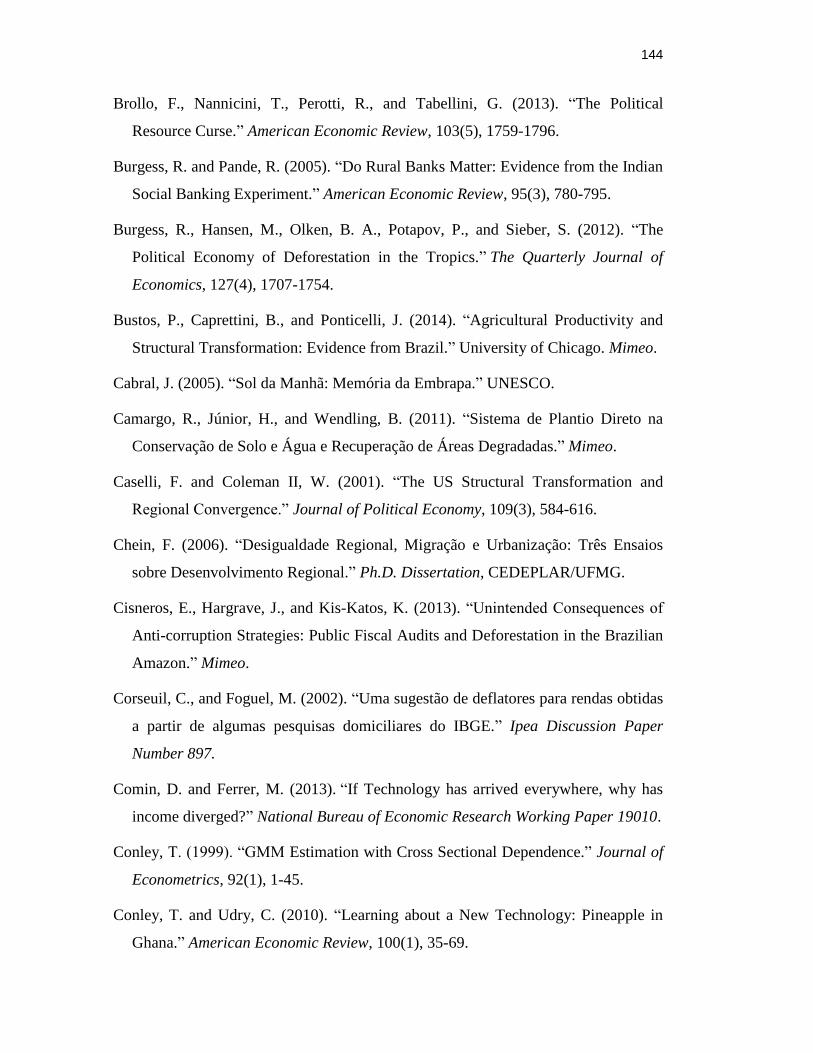
144

Brollo, F., Nannicini, T., Perotti, R., and Tabellini, G. (2013). “The Political

Resource Curse.” American Economic Review, 103(5), 1759-1796.

Burgess, R. and Pande, R. (2005). “Do Rural Banks Matter: Evidence from the Indian

Social Banking Experiment.” American Economic Review, 95(3), 780-795.

Burgess, R., Hansen, M., Olken, B. A., Potapov, P., and Sieber, S. (2012). “The

Political Economy of Deforestation in the Tropics.” The Quarterly Journal of

Economics, 127(4), 1707-1754.

Bustos, P., Caprettini, B., and Ponticelli, J. (2014). “Agricultural Productivity and

Structural Transformation: Evidence from Brazil.” University of Chicago. Mimeo.

Cabral, J. (2005). “Sol da Manhã: Memória da Embrapa.” UNESCO.

Camargo, R., Júnior, H., and Wendling, B. (2011). “Sistema de Plantio Direto na

Conservação de Solo e Água e Recuperação de Áreas Degradadas.” Mimeo.

Caselli, F. and Coleman II, W. (2001). “The US Structural Transformation and

Regional Convergence.” Journal of Political Economy, 109(3), 584-616.

Chein, F. (2006). “Desigualdade Regional, Migração e Urbanização: Três Ensaios

sobre Desenvolvimento Regional.” Ph.D. Dissertation, CEDEPLAR/UFMG.

Cisneros, E., Hargrave, J., and Kis-Katos, K. (2013). “Unintended Consequences of

Anti-corruption Strategies: Public Fiscal Audits and Deforestation in the Brazilian

Amazon.” Mimeo.

Corseuil, C., and Foguel, M. (2002). “Uma sugestão de deflatores para rendas obtidas

a partir de algumas pesquisas domiciliares do IBGE.” Ipea Discussion Paper

Number 897.

Comin, D. and Ferrer, M. (2013). “If Technology has arrived everywhere, why has

income diverged?” National Bureau of Economic Research Working Paper 19010.

Conley, T. (1999). “GMM Estimation with Cross Sectional Dependence.” Journal of

Econometrics, 92(1), 1-45.

Conley, T. and Udry, C. (2010). “Learning about a New Technology: Pineapple in

Ghana.” American Economic Review, 100(1), 35-69.

145

Costinot, A., and Donaldson, D. (2011). “How Large are the Gains from Economic

Integration? Theory and Evidence from US Agriculture, 1880-2002.”

Massachusetts Institute of Technology. Mimeo.

Costinot, A., Donaldson, D. and Smith, C. (Forthcoming). “Evolving Comparative

Advantage and the Impact of Climate Change in Agricultural Markets: Evidence

from 1.7 Million Fields across the World.” Journal of Political Economy.

Cox, G. and McCubbings, M. (1986). “Electoral Politics as a Redistributive Game,”

Journal of Politics, 48(2), 370-389.

de Almeida, L., Kiihl, R., Miranda, M., and Campelo, G. (1999). “Melhoramento de

Soja Para Regiões de Baixas Latitudes,” Embrapa. Mimeo.

de Carli, C.R. (2005). “Embrapa: precursora da parceira público-privada no Brasil,”

Master’s Dissertation. Universidade Federal de Goiás.

Derpsch, R. (1997). “Historical Review of No-Tillage Cultivation of Crops.” Mimeo.

Derpsch, R. (1999). “Frontier in Conservation Tillage and Advances in Conservation

Practice.” Mimeo.

Derpsch, R., Friedrich, T., Kassam, A., and Li, H. (2010). “Current status of

Adoption of No-till Farming in the World and Some of its Main Benefits,”

International Journal of Agricultural and Biological Engineering, 3(1): 1-25.

Diamond, J. (1997). “Guns, Germs, and Steel: The Fates of Human Societies.” W. W.

Norton and Company.

Dixit, A. and Londregan, J. (1996). “The Determinants of Success of Special Interests

in Redistributive Politics,” Journal of Politics, 58(4), 1132-1155.

Drazen, A. and Eslava, M. (2010). “Electoral Manipulation via voter-friendly

Spending: Theory and evidence,” Journal of Development Economics, 92 (1), 39–

52.

Duflo, E., Kremer, M., and Robinson, J. (2008). “How High Are Rates of Return to

Fertilizer? Evidence from Field Experiments in Kenya,” American Economic

Review Papers and Proceedings, 98(2), 482-488.

146

Duflo, E., Kremer, M., and Robinson, J. (2011). “Nudging Farmers to Use Fertilizer:

Theory and Experimental Evidence from Kenya,” American Economic Review,

101(6), 2350-90.

Durante R. (2010). “Risk, Cooperation and the Economic Origins of Social Trust: an

Empirical Investigation,” Sciences Po. Mimeo.

Ellison, G., and Fudenberg, D. (1993). “Rules of Thumb for Social Learning,”

Journal of Political Economy, 101(4), 612-643.

Esteban, J., and Ray, D. (2011). “Linking Conflict to Inequality and Polarization,”

American Economic Review, 101(4), 1345-1374.

Embrapa (2011). “O novo Mapa de Solos do Brasil.” Embrapa Solos.

Evenson, R. E., and Gollin, D. (2003). “Assessing the impact of the Green

Revolution, 1960 to 2000,” Science, 300(5620): 758-762.

Fearnside, P. M. (2001). “Land-tenure Issues as Factors in Environmental Destruction

in Brazilian Amazonia: the Case of Southern Pará,” World Development, 29(8),

1361-1372.

Fenske, J. (2014). “Ecology, Trade, and States in Pre-Colonial Africa,” Journal of the

European Economic Association, 12(3), 612-640.

Ferraz, C. (2007). “Electoral Politics and Bureaucratic Discretion: Evidence from

Environmental Licenses and Local Elections in Brazil,” PUC-Rio. Mimeo.

Ferraz, C. and Finan, F. (2008). “Exposing Corrupt Politicians: The Effects of

Brazil's Publicly Released Audits on Electoral Outcomes,” The Quarterly Journal

of Economics, 123(2), 703-745.

Ferraz, C., and Finan, F. (2009). “Motivating politicians: The impacts of monetary

incentives on quality and performance,” National Bureau of Economic Research

Working Paper 14906.

Ferraz, C. and Finan, F. (2011). “Electoral Accountability and Corruption: Evidence

from the Audits of Local Governments,” American Economic Review, 101(4),

1274-1311.

147

Firpo, S., Fortin, N., and Lemieux, T. (2009). “Unconditional Quantile

Regressions,” Econometrica, 77(3), 953-973.

Foster, A. and Rosenzweig, M. (1995). “Learning by Doing and Learning from

Others: Human Capital and Technical Change in Agriculture,” Journal of Political

Economy, 103(6), 1176:1209.

Foster, A. and Rosenzweig, M. (1996). “Technical Change and Human Capital

Returns and Investments: Evidence from the Green Revolution,” American

Economic Review, 86(4), 931-953.

Foster, A. and Rosenzweig, M. (2008). “Economic Development and the Decline of

Agricultural Employment,” Handbook of Development Economics, 4: 3051-3083.

Foster, A. and Rosenzweig, M. (2010). “Microeconomics of Technology

Adoption,” Annual Review Economics, 2(1): 395-424.

Gasques, J., Rezende, G., Villa Verde, C., Salerno, M., Conceição, J., Carvalho, J.

(2004). “Desempenho e Crescimento do Agronegócio no Brasil,” Ipea Discussion

Paper Number 1099.

Gollin, D., Lagakos, D. and Waugh, M. (2014). “The Agricultural Productivity Gap,”

The Quarterly Journal of Economics, 129(2), 939-993.

Goldstein, M. and Udry, C. (2008). “The Profits of Power: Land Rights and

Agricultural Investment in Ghana,” Journal of Political Economy, 116(6), 981-

1022.

Graham, D., Gauthier, H., and Barros, J.R. (1987). “Thirty Years of Agricultural

Growth in Brazil: Crop Performance, Regional Profile and Recent Policy Review,”

Economic Development and Cultural Change, 36(1), 1-34.

Greenstone, M., and Kack, B. K. (2013). “Envirodevonomics: A Research Agenda

for a Young Field,” Massachusetts Institute of Technology. Mimeo.

Griliches, Z. (1958). “Research Costs and Social Returns: Hybrid Corn and Related

Innovations,” Journal of Political Economy, 66, 419-431.

Grossman, G. M. and Helpman, E. (2001). “Special Interest Politics.” MIT press.

148

Guimarães, E., and Leme, H. (2002). “Caracterização Histórica e Configuração

Espacial da Estrutura Produtiva do Centro-Oeste”, Migração e Ambiente no

Centro-Oeste. Hogan D., Carmo R., Cunha, J. and Baeninger, R. (eds.). Campinas:

Editora Unicamp.

Hargrave, J., and Kis-Katos, K. (2013). “Economic causes of deforestation in the

Brazilian Amazon: A panel data analysis for the 2000s,” Environmental and

Resource Economics, 54(4), 471-494.

Helfand, S. (1999). “The Political Economy of Agricultural Policy in Brazil: Decision

Making and Influence from 1964 to 1992,” Latin American Research Review,

34(2), 3-41.

Hayami, Y. and Ruttan, V. (1970). “Factor Prices and Technical Change in

Agricultural Development: The United States and Japan, 1880-1960,” Journal of

Political Economy, 78(5), 1115-41.

Hornbeck, R. (2012). “The Enduring Impact of the American Dust Bowl: Short-and

Long-Run Adjustments to Environmental Catastrophe,” American Economic

Review, 102(4), 1477-1507.

Hornbeck, R. and Keskin, P. (2014). “The Historically Evolving Impact of the

Ogallala Aquifer: Agricultural Adaptation to Groundwater and Drought,”

American Economic Journal: Applied Economics, 6(1), 190-219.

Hornbeck, R. and Keskin, P. (Forthcoming). “Does Agriculture Generate Local

Economic Spillovers? Short-run and Long-run Evidence from the Ogallala

Aquifer,” American Economic Journal: Economic Policy.

Houtzager, P. and Kurtz, M. (1999). “The Institutional Roots of Popular

Mobilization: State Transformation and Rural Politics in Brazil and Chile, 1960-

1995,” Comparative Studies in Society and History, 42(2), 394-424.

Imbens, G., and Kalyanaraman, K. (2012). “Optimal Bandwidth Choice for the

Regression Discontinuity Estimator,” The Review of Economic Studies, 79(3), 933-

959.

149

Imbens, G. and Lemieux, T. (2008). “Regression discontinuity designs: A guide to

practice,” Journal of Econometrics, 142(2), 615-635.

Inoue, G. (2003). “Sistema de Preparo do Solo e o Plantio Direto no Brasil,”

Agropecuária Técnica, 24(1), 1-11.

IPAM (2009). “Evolução na Política para o Controle do Desmatamento na Amazônia

Brasileira: O PPCDAm,” Clima e Floresta, 15.

IPCC (2014). “Climate Change 2014: Mitigation of Climate Change,” Technical

Report, Geneva, IPCC 2014.

Ipea, Cepal, and GIZ (2011). “Avaliação do Plano de Ação para a Prevenção e

Controle do Desmatamento da Amazônia Legal,” Technical Report.

Jackson, M. (2008). “Social and Economic Networks.” Princeton University Press.

Jepson, W. (2002). “A Political Ecology of Land-Use and Land-Cover Change in the

Brazilian Savanna since 1970,” Ph.D. Dissertation, UCLA.

Jepson, W. (2006a). “Private Agricultural Colonization on a Brazilian Frontier, 1970-

1980,” Historical Geography, 32, 838-863.

Jepson, W. (2006b). “Producing a Modern Agricultural Frontier: Firms and

Cooperatives in Eastern Mato Grosso, Brazil,” Economic Geography, 82 (3), 289-

316.

Junior, M. and Vilela, L. (2002). “Pastagens no Cerrado: Baixa Produtividade pelo

Uso Limitado de Fertilizantes,” Embrapa Cerrados. Mimeo.

Karlan, D., Osei, R., Osei-Akoto, I., and Udry, C. (2014). “Agricultural Decisions

after Relaxing Credit and Risk Constraints,” The Quarterly Journal of Economics,

129(2), 597-652.

Kiihl, R. and Calvo, E. (2008). A Soja no Brasil: Mais de 100 Anos de História,

Quatro Décadas de Sucesso. Agricultural Tropical: Quatro Décadas de Inovações

Tecnológicas, Institucionais e Políticas, A. Albuquerque and A. Silva (eds.).

Embrapa Tecnologia da Informação.

150

Kindermann, G., Obersteiner, M., Sohngen, B., Sathaye, J., Andrasko, K.,

Rametsteiner, E., Schlamadinger, B., Wunder, Sven and Beach, R. (2008). “Global

Cost Estimates of Reducing Carbon Emissions through Avoided

Deforestation,” Proceedings of the National Academy of Sciences, 105(30), 10302-

10307.

Klink, C. and Moreira, A. (2002). “Past and Current Occupation and Land Use,” The

Cerrados of Brazil, P. Oliveira and R. Marquis (eds.). Columbia University Press.

Koenker, R. and Bassett, G. (1978). “Regression Quantiles,” Econometrica, 46(1):

33-50.

Lagakos, D. and Waugh, M. (2013). “Selection, Agriculture, and Cross-Country

Productivity Differences,” The American Economic Review, 103(2), 948-80.

Landers, J. (2005). “Plantio direto. Histórico, Características e Benefícios do Plantio

Direto.” Mimeo.

Leão, S., Ferraz, C., Mello, J. (2013). “Politicized Lending: Campaign Contributions

and Access to Credit,” PUC-Rio. Mimeo.

Leme, T. (2011). “Os Municípios e a Política Nacional do Meio Ambiente,”

Planejamento e Políticas Públicas, 35(2).

List, J., and Sturm, D. (2006). “How Elections Matter: Theory and Evidence from

Environmental Policy,” The Quarterly Journal of Economics, 121(4), 1249-1281.

Macêdo. M. (1998). “Pesquisadores, Agricultores e Ciência,” Cadernos de Ciência &

Tecnologia, 15(1), 29-63.

Machado, J. and Mata, J. (2005). “Counterfactual Decomposition of Changes in

Wage Distributions using Quantile Regression,” Journal of Applied

Econometrics, 20(4), 445-465.

Marden, S. (2013). “Agricultural Reforms and Growth Miracles: Evidence from

China,” London School of Economics. Mimeo.

Martinez-Bravo, M. (2014). “Educate to Lead? The Local Political Economy Effects

of School Construction in Indonesia,” Universidat Pompeu Fabra. Mimeo.

151

Matsuyama, K. (1992). “Agricultural Productivity, Comparative Advantage, and

Economic Growth,” Journal of Economic Theory, 58(2), 317-334.

McCrary, J. (2008). “Manipulation of the Running Variable in the Regression

Discontinuity Design: A density test,” Journal of Econometrics, 142(2), 698-714.

Metay, A., Oliver, R. Scopel, E., Douzet, J-M., Moreira, J., Maraux, F., Feigl, B. and

Feller, C. (2007). “N2O and CH4 Emissions from Soils under Conventional and

No-till Management Practices in Goiânia (Cerrados, Brazil),” Geoderma, 141 (1–

2): 78-88.

Mian, A., Sufi, A. and Trebbi, F. (2010). “The Political Economy of the US Mortgage

Default Crisis,” American Economic Review, 100(5), 1967-98.

Michalopoulos, S. (2012). “The Origins of Ethnolinguistic Diversity,” American

Economic Review, 102(4), 1508-39.

Monteiro, J., Rocha, A., and Kury, B. (2012). “Soybeans in the Savannahs of Brazil,”

Export Pioneers in Latin American, C. Sabel, E. Férnandez-Arias, R. Hausmann,

A. Rodriguez-Clare and E. Stein (eds.). Inter-American Development Bank.

Morjaria, A. (2013). “Electoral Competition and Deforestation: Evidence from

Kenya,” London School of Economics. Mimeo.

Munshi, K. (2004). “Social Learning in a Heterogeneous Population: Technology

Diffusion in the Indian Green Revolution,” Journal of Development Economics,

73(1), 185-213.

Ngai, L. and Pissarides, C. (2007). “Stuctural Change in a Multisector Model of

Growth,” American Economic Review, 97(1), 429-443.

Nunn, N., and Qian, N. (2011). “The Potato's Contribution to Population and

Urbanization: Evidence from a Historical Experiment,” The Quarterly Journal of

Economics, 126(2), 593-650.

Oliveira, P. and Marquis, R. (2002). “The Cerrados of Brazil: Ecology and Natural

History of a Neotropical Savanna.” Columbia University Press.

152

Olmstead, A., and Rhode, P. (2001). “Reshaping the Landscape: the Impact and

Diffusion of the Tractor in American Agriculture, 1910–1960,” The Journal of

Economic History, 61(03), 663-698.

Olmstead, A., and Rhode, P. (2008). “Creating Abundance: Biological Innovation

and American Agricultural Development.” Cambridge: Cambridge University

Press.

Osborne, M. J. and Slivinski, A. (1996). “A Model of Political Competition with

Citizen-Candidates,” The Quarterly Journal of Economics, 111(1), 65-96.

Persson, T. and Tabellini, G. (2002). “Political Economics: Explaining Economic

Policy.” MIT Press.

Pfaff, A. (1999). “What drives deforestation in the Brazilian Amazon? Evidence from

Satellite and Socioeconomic Data,” Journal of Environmental Economics and

Management, 37(1), 26-43.

Pfaff, A.; Robalino, J., Walker, R., Aldrich, S. Caldas, Reis, E., M., Perz, S., Bohrer,

C., Arima, E., Laurance, W. et al (2007). “Road Investments, Spatial Spillovers,

and Deforestation in the Brazilian Amazon,” Journal of Regional Science, 47(1),

109-123.

Piedra, N. (2013). “Legislative Hurdles to Agrarian Reform: The Role of the Bancada

Ruralista in the Brazilian Chamber of Deputies, 1995-2006,” Harvard University.

Mimeo.

PRODES (2013). “Metodologia para Cálculo da Taxa Anual de Desmatamento na

Amazônia Legal.” Technical Report. São José dos Campos: INPE (available at

obt.inpe.br/prodes/metodologia_TaxaProdes.pdf).

Rada, N. (2013). “Assessing Brazil’s Cerrado Agricultural Miracle,” Food Policy,

38(C), 146-155.

Rada, N. and Buccola, S. (2012). “Agricultural policy and productivity: evidence

from Brazilian censuses,” Agricultural Economics, 43(4), 355-367.

153

Rezende, G. (2002). “Ocupação Agrícola e Estrutura Agrária no Cerrado,” IPEA

Discussion Paper Number 913.

Richardson, N. P. (2012). “The Politics of Abundance: Export Agriculture and

Redistributive Conflict in South America,” Ph.D. Dissertation, University of

California (Berkeley).

Rigotti, J., Rios-Neto, E., and Riani, J. (2004). “Variáveis de Educação dos Censos

Demográficos Brasileiros de 1960 a 2000,” Introdução à Demografia da

Educação. ABEP.

Ringler, C., Cenacchi, N., Koo, J., Robertson, R., Fisher, M., Cox, C., Perez, N.,

Garrett, K. and Rosengran, M. (2013). “The Promise of Innovative Farming

Practices,” Global Food Policy Report, IFPRI (eds.), International Food Policy

Research Institute.

Rogoff, K. (1990). “Equilibrium Political Budget Cycles,” American Economic

Review, 80(1), 21-36.

Salim, C. (1986). “As Políticas Econômica e Tecnológica para o Desenvolvimento

Agrário das Áreas de Cerrados no Brasil: Avaliação e Perspectivas,” Caderno de

Difusão de Tecnologia, 3(2), 297-342.

Sanders, J., and Bein, F. (1976). “Agricultural Development on the Brazilian

Frontier: Southern Mato Grosso,” Economic Development and Cultural Change,

24(3), 593-610.

Santos (2006). “Sistema Brasileiro de Conservação de Solos.” Embrapa Solos.

Santos, M., Barbieri, A., Guedes, G., Machado, C., and Carvalho, J.. (2012).

“Dinâmica Demográfica e Uso da Terra no Cerrado Brasileiro: Reflexões a partir

da Experiência do Padap,” Revista de Economia e Sociologia Rural, 50(2), 319-

331.

Schultz, T. (1953). “The Economic Organization of Agriculture.” New York:

McGraw-Hill.

154

Souza-Rodrigues, E. (2013). “Demand for Deforestation in the Amazon,” University

of Toronto. Mimeo.

Sorrenson, W. and Portillo, J. (1997). “Paraguay Soil Conservation Project:

Economic of No-tillage and Crop Rotations Policy and Investment Implications.”

Mimeo.

Spehar, C. (1994). “Impact of Strategic Genes of Soybean on Agricultural

Development in the Brazilian Tropical Savannahs,” Field Crops Research, 41, 41-

46.

Stern, N. (2007). “The Economics of Climate Change: The Stern Review.” Cambridge

University Press.

Strauss, J., Barbosa, M., Teixeira, S., Thomas, D., and Gomes Júnior, R. (1991). “The

Role of Education and Extension in the Adoption of Technology: a Study of Up-

land Rice and Soybean Farmers in Central-West Brazil,” Agricultural Economics,

5: 341-359.

Sukhtankar, S. (2012). “Sweetening the Deal? Political Connections and Sugar Mills

in India,” American Economic Journal: Applied Economics, 4(3), 43-63.

Suri, T. (2011). “Selection and Comparative Advantage in Technology Adoption,”

Econometrica, 79(1), 159-209.

Testa, V., Teixeira, L., Mielniczuk, J. (1992). “Características Químicas de um

Podzólico Vermelho-Escuro afetadas por sistemas de culturas,” Revista Brasileira

de Ciência do Solo, 16(1): 107-114.

The Economist (2012). “Environmental Law in Brazil: Compromise or Deadlock?,”

The Economist, June 2nd.

Trigo, E., Cap, E., Malach, V., Villareal, F. (2009). “The Case of Zero-Tillage

Technology in Argentina,” IFPRI Discussion Paper 915.

Udry, C. (2010). “The Economics of Agriculture in Africa: Notes toward a Research

Programme,” African Journal of Agricultural and Resource Economics, 5(1), 284-

299.

155

Welch, F. (1970). “Education in Production,” Journal of Political Economy, 78(1),

35-59.

West, T. O., and Post, W. M. (2002). “Soil Organic Carbon Sequestration Rates by

Tillage and Crop Rotation,” Soil Science Society of America Journal, 66(6), 1930-

1946.

Young, H. (2009). “Innovation Diffusion in Heterogeneous Populations: Contagion,

Social Influence, and Social Learning,” American Economic Review, 99(5), 1899-

1924.

Young, A. (2013). “Inequality, the Urban-Rural Gap, and Migration,” The Quarterly

Journal of Economics, 128(4), 1727-1785.