Universidad Nacional de La Plata
Séptimas Jornadas de EconomíaMonetaria e InternacionalLa Plata, 9 y 10 de mayo de 2002
The Term Structure of Country Risk and Valuation inEmerging Markets
Cruces, Juan José (Universidad de San Andrés), Buscaglia, Marcos(IAE School of Management and Business, Universidad Austral)
and Alonso, Joaquín (Mercado Abierto)
The Term Structure of Country Risk
and Valuation in Emerging Markets
Juan José Cruces† Marcos Buscaglia†† Joaquín Alonso‡
First draft: January 2002
AbstractMost practitioners add the country risk to the discount rate when valuing projects in Emerging Markets. In
addition to the problems already pointed out in the literature, in this paper we claim that such practice leads to
a pro-cyclical bias in the valuation of long-term projects. The mismatch between the duration of the project
and the duration of the most widely used measure of country risk, J.P. Morgan’s EMBI, leads to an
overvaluation of long-term projects in good times (upward sloping default risk) and to an undervaluation of
them when short-term default risk is high (the contrary is true with respect to short-term projects.)
Using sovereign bond data from five Emerging Markets, we estimate a simple model that captures most of the
variation of default probabilities at different horizons for a given country at one point in time. This model can
be used to solve the misestimation problem.
JEL classification codes: G15, G31
Keywords : Emerging Economies, Cost of Capital, Default Risk
† Universidad de San Andrés, Victoria, Province of Buenos Aires, Argentina. E-mail address:
†† IAE School of Management and Business, Universidad Austral, Pilar, Province of Buenos Aires, Argentina.
Tel.: 54-2322-481069. E-mail address: [email protected]. Corresponding author.
‡ Mercado Abierto, S.A., Buenos Aires, Argentina. E-mail address: [email protected].
2
I. Introduction
Projects in emerging markets are generally perceived as riskier than otherwise similar
projects in developed countries. These “additional risks” include currency inconvertibility,
civil unrest, institutional instability, expropriation, and widespread corruption. Emerging
markets (henceforth EM) are also more volatile than developed economies: their business
cycles are more intense1, and inflation and currency risks are higher.
Several problems have restricted the use among practitioners of the Capital Asset Pricing
Model (CAPM) or its international version, the ICAPM2, to calculate the cost of capital of
projects in EM. First, there is no complete agreement about the degree of integration of EM
capital markets to the world market (see Errunza and Losq, 1985, and Bekaert et al., 2001).
Secondly, local returns are non-normal, show significant first-order autocorrelation
(Bekaert et al., 1998), and there are problems of liquidity and infrequent trading. Finally, as
correlations between local returns and international returns are so low (see Harvey, 1995),
the cost of capital that emerges from the use of these models appears as “too low”.
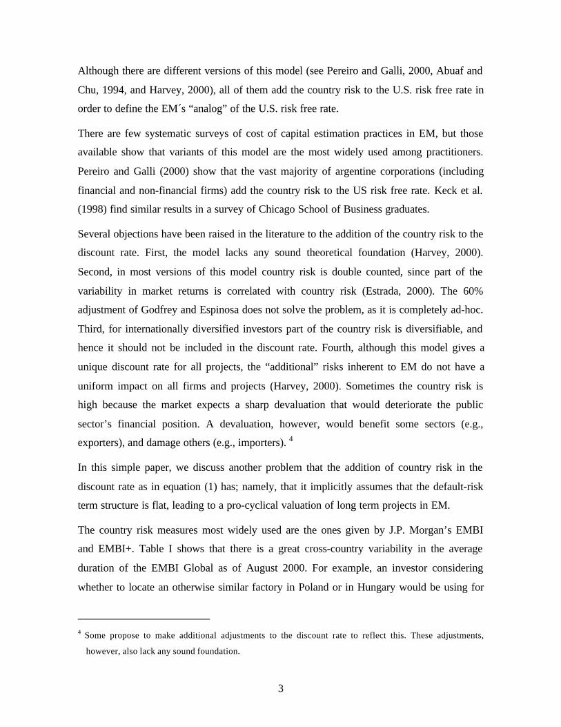
These problems have lead practitioners to account for the “additional risks” by making ad
hoc adjustments to the CAPM. Godfrey and Espinosa (1996), for instance, propose to
calculate the cost of capital in EM by using
E[Ri ]= ( RfUS
+ Credit Spread ) + US
i
σσ
* 0.60 * ( E[RmUS ]– Rf
US ) (1)
where credit spread is the spread between the yield of a U.S. Dollar-denominated EM
sovereign bond and the yield of a comparable U.S. bond, and the term preceding the last
parenthesis is an “adjusted beta”, that is equivalent to 60% of the ratio of the volatility of
the domestic market to that of the U.S. market.3
1 Neumeyer and Perri (2001) find that output in Argentina, Brazil, Korea, Mexico and Philippines is at least
twice as volatile as it is in Canada.
2 See Adler and Dumas (1983).
3 The 60% adjustment is due to the finding that 40% of the volatilities of domestic markets are explained by
variations in credit quality.
3
Although there are different versions of this model (see Pereiro and Galli, 2000, Abuaf and
Chu, 1994, and Harvey, 2000), all of them add the country risk to the U.S. risk free rate in
order to define the EM´s “analog” of the U.S. risk free rate.
There are few systematic surveys of cost of capital estimation practices in EM, but those
available show that variants of this model are the most widely used among practitioners.
Pereiro and Galli (2000) show that the vast majority of argentine corporations (including
financial and non-financial firms) add the country risk to the US risk free rate. Keck et al.
(1998) find similar results in a survey of Chicago School of Business graduates.
Several objections have been raised in the literature to the addition of the country risk to the
discount rate. First, the model lacks any sound theoretical foundation (Harvey, 2000).
Second, in most versions of this model country risk is double counted, since part of the
variability in market returns is correlated with country risk (Estrada, 2000). The 60%
adjustment of Godfrey and Espinosa does not solve the problem, as it is completely ad-hoc.
Third, for internationally diversified investors part of the country risk is diversifiable, and
hence it should not be included in the discount rate. Fourth, although this model gives a
unique discount rate for all projects, the “additional” risks inherent to EM do not have a
uniform impact on all firms and projects (Harvey, 2000). Sometimes the country risk is
high because the market expects a sharp devaluation that would deteriorate the public
sector’s financial position. A devaluation, however, would benefit some sectors (e.g.,
exporters), and damage others (e.g., importers). 4
In this simple paper, we discuss another problem that the addition of country risk in the
discount rate as in equation (1) has; namely, that it implicitly assumes that the default-risk
term structure is flat, leading to a pro-cyclical valuation of long term projects in EM.
The country risk measures most widely used are the ones given by J.P. Morgan’s EMBI
and EMBI+. Table I shows that there is a great cross-country variability in the average
duration of the EMBI Global as of August 2000. For example, an investor considering
whether to locate an otherwise similar factory in Poland or in Hungary would be using for
4 Some propose to make additional adjustments to the discount rate to reflect this. These adjustments,
however, also lack any sound foundation.
4
Poland a country spread corresponding to a duration of 6 years, whereas in Hungary he
would be using a spread associated with a duration of 2.3 years.
Using these default-risk measures in the discount rate to value long-term projects would
bear no additional problem to the ones mentioned above if the default-risk term structure
were flat. But, in fact, this is not the case. In good times, when capital is flowing to EM,
risk spreads are low at the short end of the curve, but they are upward sloping. In many
instances, moreover, the default-risk term structure is downward sloping. This usually
happens when the market expects a default in the short term.
The mismatch between the duration of the project and the duration of the EMBI leads to an
overvaluation of long-term projects in good times and to an undervaluation of them when
default risk is high (the contrary is true with respect to short term projects.)
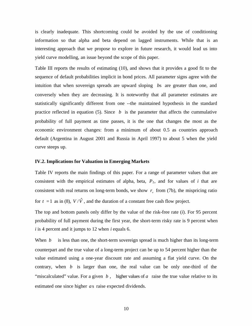
Figure I.A. illustrates this point. While in August 2001 Mexico and Russia had similar
spreads on bonds with short durations, Russia´s risk was much higher at longer horizons. A
mechanical application of equation (1) would ignore these data, which are readily available
from bond markets, and would have led to an undervaluation of otherwise similar long-term
projects in Mexico relative to Russia.
Using sovereign bond data from five Emerging Markets, in this paper we estimate a simple
model that captures most of the variation of default probabilities at different horizons for a
given country at one point in time. This model can be used to solve the miss-estimation
problem.
The paper proceeds as follows. In Section II we explain the model we use to estimate the
default-risk term structure in EM sovereign debt markets and discuss the effects that a non-
flat default-risk term structure has on the valuation of projects. In Section III we describe
the data used to estimate the model. In Section IV we present the estimation results. Section
V concludes.
II. The Model
Consider a perpetuity that promises to pay a coupon of $ c every period (a period represents
one year for simplicity). Let it be the expected annual rate of return on this bond from
5
period zero up to period t, γ the recovery value conditional on default, pt the period-t
probability of payment conditional on previous full payment, and Pt the probability of
payment t-periods from now. Given that each coupon payment has “cross-default”
provisions with every successive coupon, Pt measures the cumulative probability of no
default from inception up to period t.
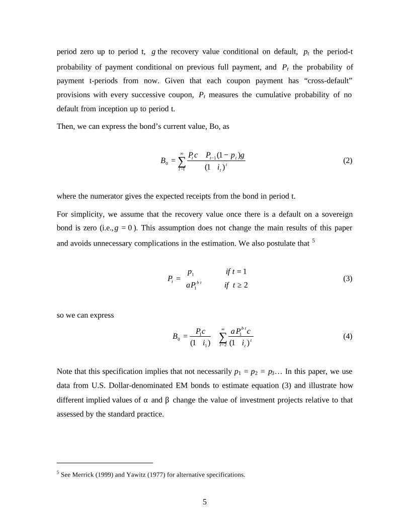
Then, we can express the bond’s current value, Bo, as
∑∞
=
−
+−+
=1
10
)1(
)1(
tt
t
ttt
i
pPcPB
γ (2)
where the numerator gives the expected receipts from the bond in period t.
For simplicity, we assume that the recovery value once there is a default on a sovereign
bond is zero (i.e., 0=γ ). This assumption does not change the main results of this paper
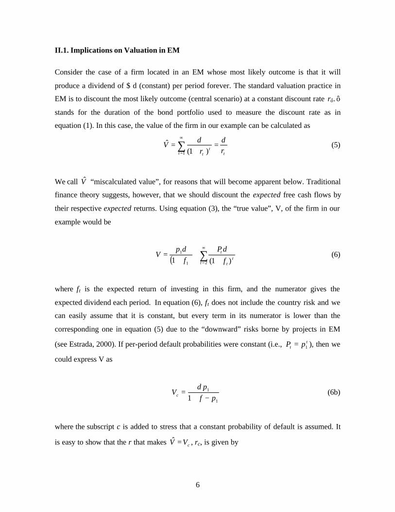
and avoids unnecessary complications in the estimation. We also postulate that 5
≥
==
2
1
1
1
tifP
tifpP
tt βα (3)
so we can express
∑∞
= ++
+=
2
1
1
10
)1()1( tt
t
t
i
cP
i
cPB
βα (4)
Note that this specification implies that not necessarily p1 = p2 = p3… In this paper, we use
data from U.S. Dollar-denominated EM bonds to estimate equation (3) and illustrate how
different implied values of α and β change the value of investment projects relative to that
assessed by the standard practice.
5 See Merrick (1999) and Yawitz (1977) for alternative specifications.
6
II.1. Implications on Valuation in EM
Consider the case of a firm located in an EM whose most likely outcome is that it will
produce a dividend of $ d (constant) per period forever. The standard valuation practice in
EM is to discount the most likely outcome (central scenario) at a constant discount rate rô. ô
stands for the duration of the bond portfolio used to measure the discount rate as in
equation (1). In this case, the value of the firm in our example can be calculated as
ττ rd
r
dV
tt
=+
= ∑∞
=1 )1(ˆ (5)
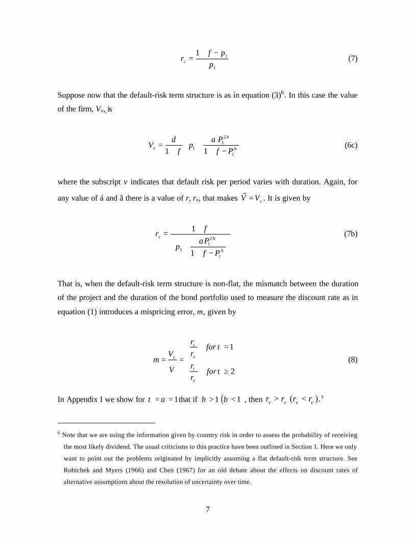
We call V̂ “miscalculated value”, for reasons that will become apparent below. Traditional
finance theory suggests, however, that we should discount the expected free cash flows by
their respective expected returns. Using equation (3), the “true value”, V, of the firm in our
example would be
( ) ∑∞
= ++
+=
21
1
)1(1 tt
t
t
f
dP
f
dpV (6)
where ft is the expected return of investing in this firm, and the numerator gives the
expected dividend each period. In equation (6), ft does not include the country risk and we
can easily assume that it is constant, but every term in its numerator is lower than the
corresponding one in equation (5) due to the “downward” risks borne by projects in EM
(see Estrada, 2000). If per-period default probabilities were constant (i.e., tt pP 1= ), then we
could express V as
1
1
1 pf
pdVc −+
= (6b)
where the subscript c is added to stress that a constant probability of default is assumed. It
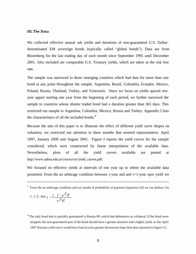
is easy to show that the r that makes cVV =ˆ , rc, is given by
7
1
11
p
pfrc
−+= (7)
Suppose now that the default-risk term structure is as in equation (3)6. In this case the value
of the firm, Vv,,is
−++
+= β
βα
1
21
1 11 Pf
Pp
f
dVv (6c)
where the subscript v indicates that default risk per period varies with duration. Again, for
any value of á and â there is a value of r, rv, that makes vVV =ˆ . It is given by
−+
+
+=
β
βα
1
21
11
1
Pf
Pp
frv (7b)
That is, when the default-risk term structure is non-flat, the mismatch between the duration
of the project and the duration of the bond portfolio used to measure the discount rate as in
equation (1) introduces a mispricing error, m, given by
≥
===
∧
2
1
τ
τ
τ forr
r
forr
r
V
Vm
v
v
c
v (8)
In Appendix I we show for 1== ατ that if ( )11 <> ββ , then ).( cvcv rrrr <> 7
6 Note that we are using the information given by country risk in order to assess the probability of receiving
the most likely dividend. The usual criticisms to this practice have been outlined in Section 1. Here we only
want to point out the problems originated by implicitly assuming a flat default-risk term structure. See
Robichek and Myers (1966) and Chen (1967) for an old debate about the effects on discount rates of
alternative assumptions about the resolution of uncertainty over time.
8
III. The Data
We collected effective annual ask yields and durations of non-guaranteed U.S. Dollar-
denominated EM sovereign bonds (typically called “global bonds”). Data are from
Bloomberg for the last trading day of each month since September 1995 until December
2001. Also included are comparable U.S. Treasury yields, which are taken as the risk free
rate.
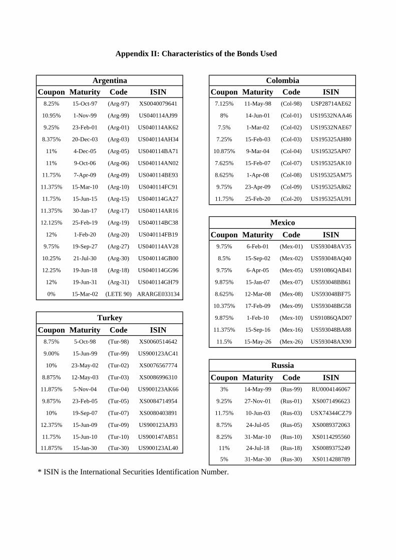
The sample was narrowed to those emerging countries which had data for more than one
bond at any point throughout the sample: Argentina, Brazil, Colombia, Ecuador, Mexico,
Poland, Russia, Thailand, Turkey, and Venezuela. Since we focus on yields spaced one-
year appart starting one year from the beginning of each period, we further narrowed the
sample to countries whose shorter traded bond had a duration greater than 365 days. This
restricted our sample to Argentina, Colombia, Mexico, Russia and Turkey. Appendix I lists
the characteristics of all the included bonds.8
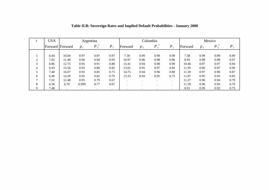
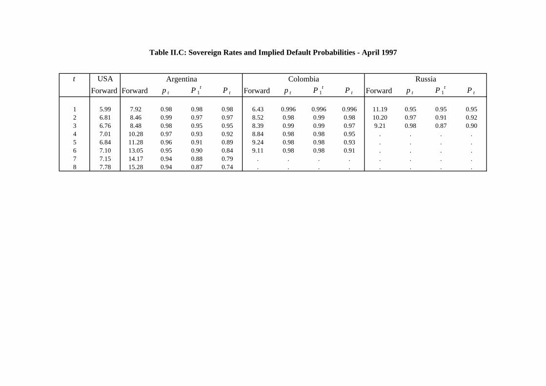
Because the aim of this paper is to illustrate the effect of different yield curve shapes on
valuation, we restricted our attention to three months that seemed representative: April
1997, January 2000 and August 2001. Figure I reports the yield curves for the sample
considered, which were constructed by linear interpolation of the available data.
Nevertheless, plots of all the yield curves available are posted at
http://www.udesa.edu.ar/cruces/coc/yield_curves.pdf.
We focused on effective yields at intervals of one year up to where the available data
permitted. From the no arbitrage condition between t-year and and t+1-year spot yield we
7 From the no arbitrage condition and our model of probability of payment [equation (3)] we can deduce, for
2≥τ , that βτ
βτ
τα
α
1
11
1
1
P
Pfr
−+= .
8 The only bond that is partially guaranteed is Russia-99, which had debentures as collateral. If the bond were
stripped, the non-guaranteed part of the bond should have a greater duration and a higher yield, so the April
1997 Russian yield curve would have had an even greater downward slope than that reported in Figure I.C.
9
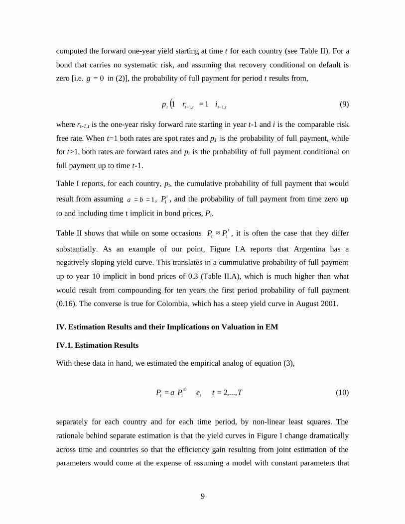
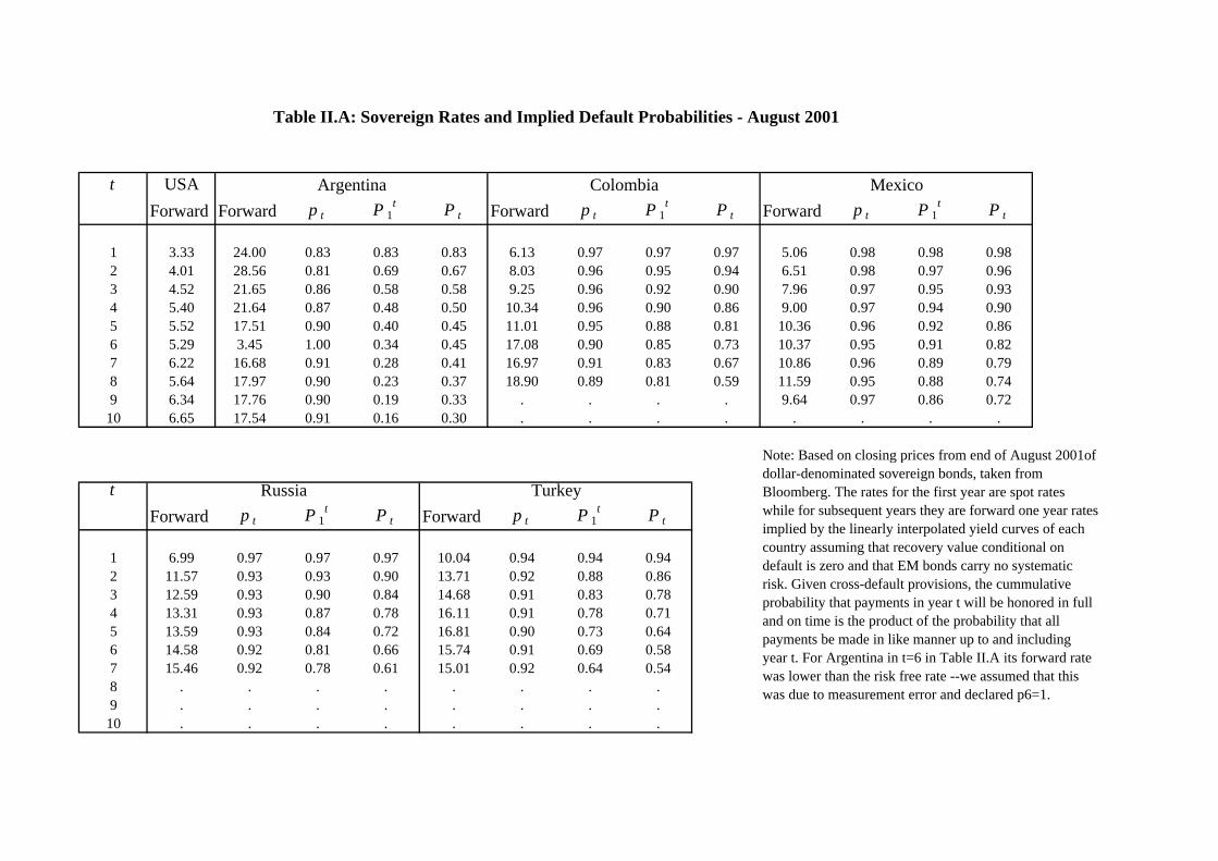
computed the forward one-year yield starting at time t for each country (see Table II). For a
bond that carries no systematic risk, and assuming that recovery conditional on default is
zero [i.e. 0=γ in (2)], the probability of full payment for period t results from,
( ) ttttt irp ,1,1 11 −− +=+ (9)
where rt-1,t is the one-year risky forward rate starting in year t-1 and i is the comparable risk
free rate. When t=1 both rates are spot rates and p1 is the probability of full payment, while
for t>1, both rates are forward rates and pt is the probability of full payment conditional on
full payment up to time t-1.
Table I reports, for each country, pt, the cumulative probability of full payment that would
result from assuming 1== βα , tP1 , and the probability of full payment from time zero up
to and including time t implicit in bond prices, Pt.
Table II shows that while on some occasions t
t PP 1≈ , it is often the case that they differ
substantially. As an example of our point, Figure I.A reports that Argentina has a
negatively sloping yield curve. This translates in a cummulative probability of full payment
up to year 10 implicit in bond prices of 0.3 (Table II.A), which is much higher than what
would result from compounding for ten years the first period probability of full payment
(0.16). The converse is true for Colombia, which has a steep yield curve in August 2001.
IV. Estimation Results and their Implications on Valuation in EM
IV.1. Estimation Results
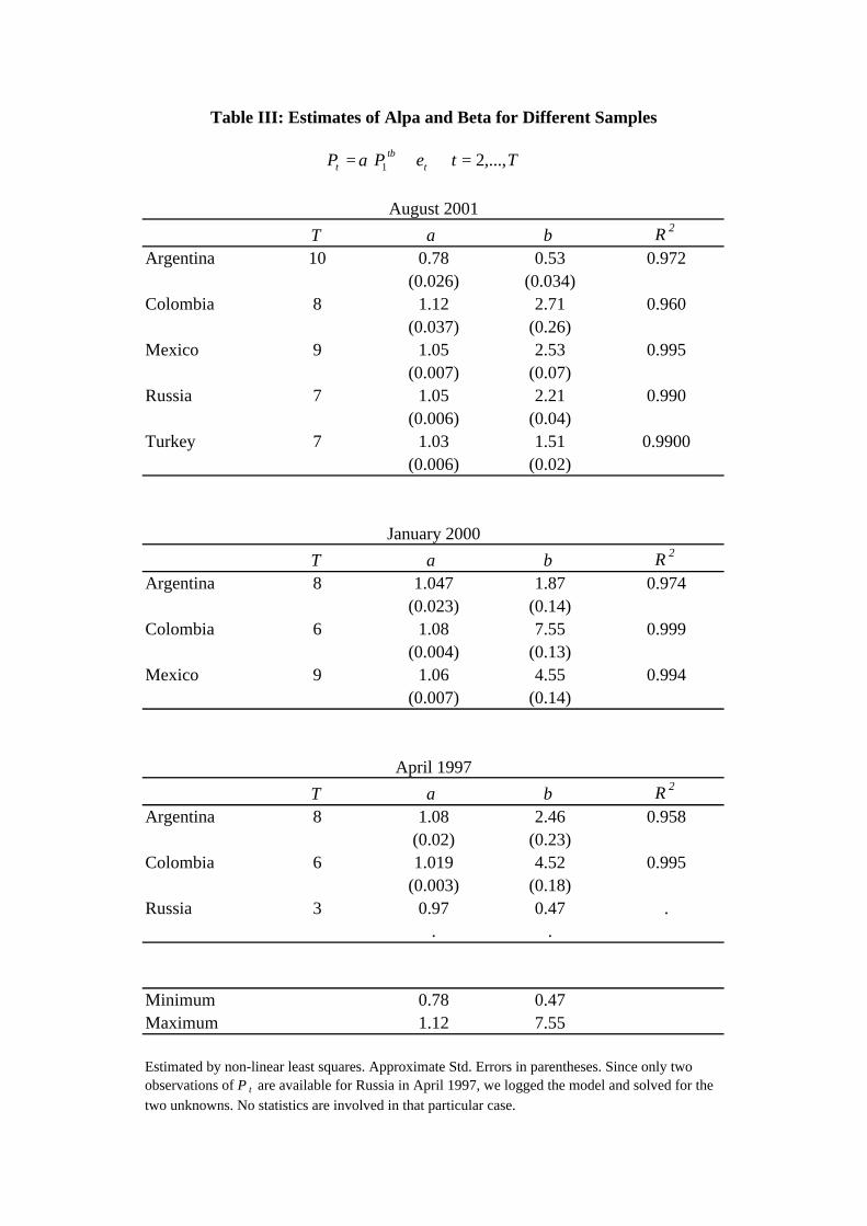
With these data in hand, we estimated the empirical analog of equation (3),
TtePP t
t
t ,...,21 =+= βα (10)
separately for each country and for each time period, by non-linear least squares. The
rationale behind separate estimation is that the yield curves in Figure I change dramatically
across time and countries so that the efficiency gain resulting from joint estimation of the
parameters would come at the expense of assuming a model with constant parameters that
10
is clearly inadequate. This shortcoming could be avoided by the use of conditioning
information so that alpha and beta depend on lagged instruments. While that is an
interesting approach that we propose to explore in future research, it would lead us into
yield curve modelling, an issue beyond the scope of this paper.
Table III reports the results of estimating (10), and shows that it provides a good fit to the
sequence of default probabilities implicit in bond prices. All parameter signs agree with the
intuition that when sovereign spreads are upward sloping sβ are greater than one, and
conversely when they are decreasing. It is noteworthy that all parameter estimates are
statistically significantly different from one --the maintained hypothesis in the standard
practice reflected in equation (5). Since β is the parameter that affects the cummulative
probability of full payment as time passes, it is the one that changes the most as the
economic environment changes: from a minimum of about 0.5 as countries approach
default (Argentina in August 2001 and Russia in April 1997) to about 5 when the yield
curve steeps up.
IV.2. Implications for Valuation in Emerging Markets
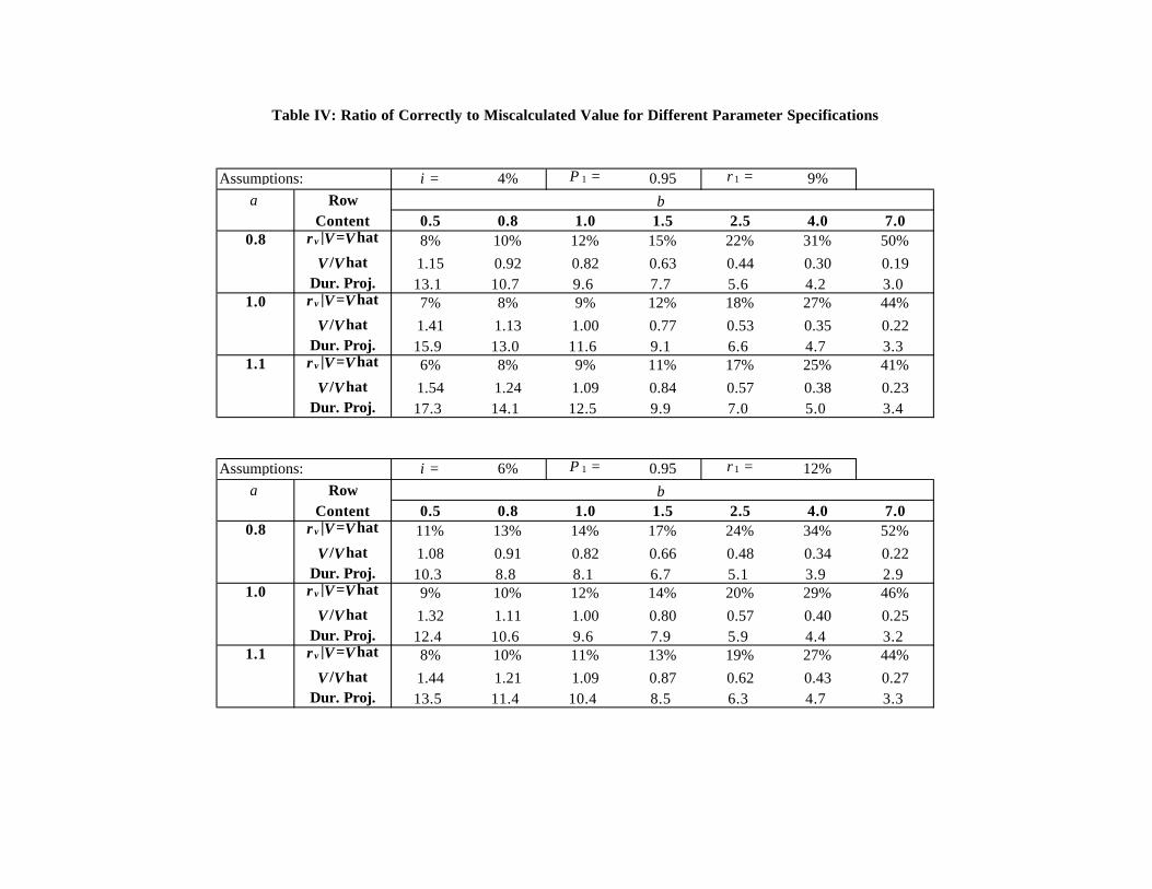
Table IV reports the main findings of this paper. For a range of parameter values that are
consistent with the empirical estimates of alpha, beta, P1, and for values of i that are
consistent with real returns on long-term bonds, we show vr from (7b), the mispricing ratio
for 1=τ as in (8), VV ˆ/ , and the duration of a constant free cash flow project.
The top and bottom panels only differ by the value of the risk-free rate (i). For 95 percent
probability of full payment during the first year, the short-term risky rate is 9 percent when
i is 4 percent and it jumps to 12 when i equals 6.
When β �is less than one, the short-term sovereign spread is much higher than its long-term
counterpart and the true value of a long-term project can be up to 54 percent higher than the
value estimated using a one-year discount rate and assuming a flat yield curve. On the
contrary, when β is larger than one, the real value can be only one-third of the
“miscalculated” value. For a given β , �higher values of α raise the true value relative to its
estimated one since higher sα raise expected dividends.

11
Naturally, when the yield curve steeps up, the constant discount rate that would make the
value of the project from (5) equal to that of (6) is much higher than the short term rate.
V. Conclusions and Further Research
Several problems have restricted practitioners from using the CAPM in order to estimate
discount rates in Emerging Markets, and have led them to account for the “additional” risks
of EM by adding the country risk to the discount rate.
In this paper we claim that such practice does not make an efficient use of the information
given by sovereign debt markets. In particular, it does not account for the fact that the
default-risk term structure is non-flat, being upward sloping in good times, and downward
sloping when the short-term default risk is high.
The mismatch between the duration of the project and the duration of the most widely used
measures of country risk, J.P. Morgan’s EMBI, leads to an overvaluation of long-term
projects in good times and to an undervaluation of them when default risk is high (the
contrary is true with respect to short term projects.)
In this paper, using data from five EM, we estimate a simple model of the term structure of
default-risk and derive its implications on valuation.
We find that by implicitly assuming that the term structure of default risk is flat, mispricing
errors in the range of plus or minus 50 percent can be made for reasonable parameter
values. This mispricing can be avoided by using data that are readily available from bond
markets.
To enrich the analysis, future research should be directed to the inclusion of recovery
values and the use of conditioning information in a model of default-risk term structure.
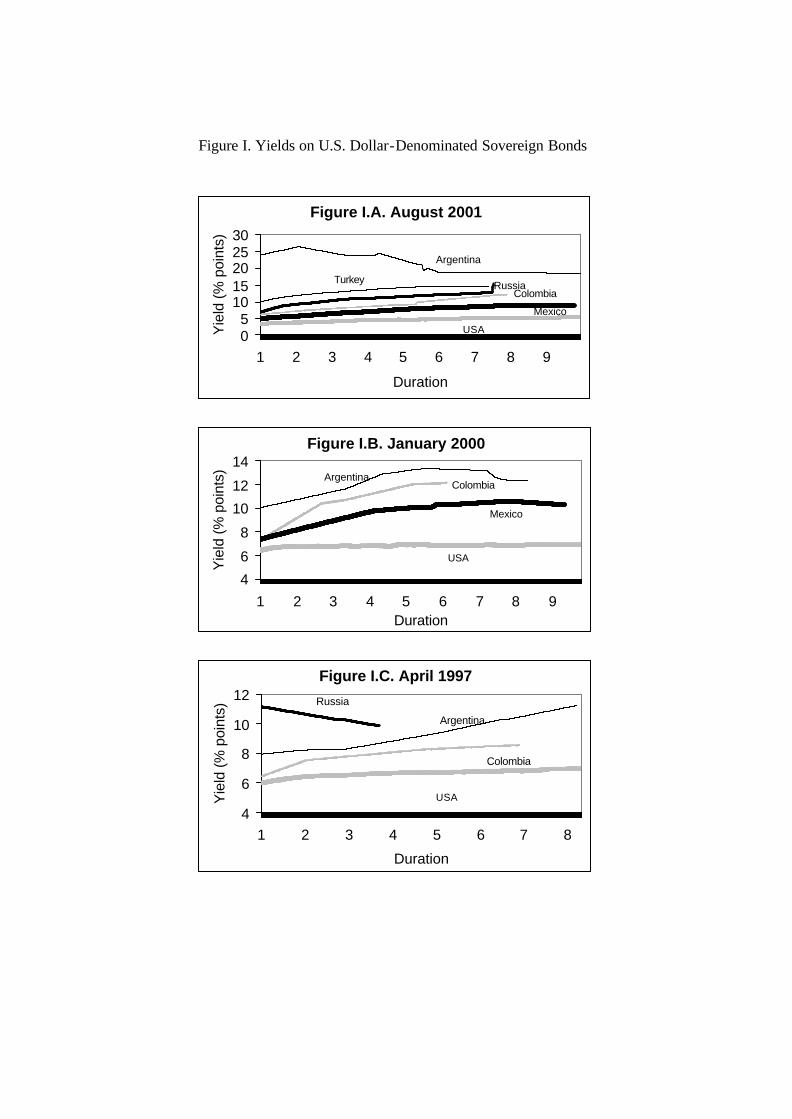
Figure I. Yields on U.S. Dollar-Denominated Sovereign Bonds
Figure I.A. August 2001
05
1015202530
1 2 3 4 5 6 7 8 9
Duration
Yie
ld (%
poi
nts)
Argentina
USA
Mexico
ColombiaRussiaTurkey
Figure I.B. January 2000
4
6
8
10
12
14
1 2 3 4 5 6 7 8 9Duration
Yie
ld (%
poi
nts) Argentina
USA
Mexico
Colombia
Figure I.C. April 1997
4
6
8
10
12
1 2 3 4 5 6 7 8
Duration
Yie
ld (%
poi
nts)
Argentina
USA
Colombia
Russia
Country DurationAlgeria 3.05Argentina 4.13Brazil 4.94Bulgaria 4.59Chile 6.20China 4.56Colombia 5.40Cote d'Ivore 6.20Croatia 3.80Ecuador 5.90Hungary 2.33Lebanon 2.30Malaysia 4.93Mexico 4.93Morocco 3.24Nigeria 1.92Panama 6.56Peru 7.02Philippines 7.14Poland 6.01Russia 5.78South Africa 6.53South Korea 3.79Thailand 4.98Turkey 5.95Ukraine 2.59Venezuela 4.15
Mean 4.77Standard Deviation 1.52
Source: J.P. Morgan (2000)
Table I: Average Duration of Country Components ofJP Morgan's EMBI Global Index
t USA
Forward Forward p t P 1t P t Forward p t P 1
t P t Forward p t P 1t P t
1 3.33 24.00 0.83 0.83 0.83 6.13 0.97 0.97 0.97 5.06 0.98 0.98 0.982 4.01 28.56 0.81 0.69 0.67 8.03 0.96 0.95 0.94 6.51 0.98 0.97 0.963 4.52 21.65 0.86 0.58 0.58 9.25 0.96 0.92 0.90 7.96 0.97 0.95 0.934 5.40 21.64 0.87 0.48 0.50 10.34 0.96 0.90 0.86 9.00 0.97 0.94 0.905 5.52 17.51 0.90 0.40 0.45 11.01 0.95 0.88 0.81 10.36 0.96 0.92 0.866 5.29 3.45 1.00 0.34 0.45 17.08 0.90 0.85 0.73 10.37 0.95 0.91 0.827 6.22 16.68 0.91 0.28 0.41 16.97 0.91 0.83 0.67 10.86 0.96 0.89 0.798 5.64 17.97 0.90 0.23 0.37 18.90 0.89 0.81 0.59 11.59 0.95 0.88 0.749 6.34 17.76 0.90 0.19 0.33 . . . . 9.64 0.97 0.86 0.72
10 6.65 17.54 0.91 0.16 0.30 . . . . . . . .
t
Forward p t P 1t P t Forward p t P 1
t P t
1 6.99 0.97 0.97 0.97 10.04 0.94 0.94 0.942 11.57 0.93 0.93 0.90 13.71 0.92 0.88 0.863 12.59 0.93 0.90 0.84 14.68 0.91 0.83 0.784 13.31 0.93 0.87 0.78 16.11 0.91 0.78 0.715 13.59 0.93 0.84 0.72 16.81 0.90 0.73 0.646 14.58 0.92 0.81 0.66 15.74 0.91 0.69 0.587 15.46 0.92 0.78 0.61 15.01 0.92 0.64 0.548 . . . . . . . .9 . . . . . . . .
10 . . . . . . . .
Note: Based on closing prices from end of August 2001of dollar-denominated sovereign bonds, taken from Bloomberg. The rates for the first year are spot rates while for subsequent years they are forward one year rates implied by the linearly interpolated yield curves of each country assuming that recovery value conditional on default is zero and that EM bonds carry no systematic risk. Given cross-default provisions, the cummulative probability that payments in year t will be honored in full and on time is the product of the probability that all payments be made in like manner up to and including year t. For Argentina in t=6 in Table II.A its forward rate was lower than the risk free rate --we assumed that this was due to measurement error and declared p6=1.
Russia Turkey
Table II.A: Sovereign Rates and Implied Default Probabilities - August 2001
Argentina Colombia Mexico
t USA
Forward Forward p t P 1t P t Forward p t P 1
t P t Forward p t P 1t P t
1 6.44 10.04 0.97 0.97 0.97 7.30 0.99 0.99 0.99 7.38 0.99 0.99 0.992 7.02 11.40 0.96 0.94 0.93 10.97 0.96 0.98 0.96 8.95 0.98 0.98 0.973 6.86 12.75 0.95 0.91 0.88 13.41 0.94 0.98 0.90 10.46 0.97 0.97 0.944 6.93 15.56 0.93 0.88 0.82 13.01 0.95 0.97 0.85 11.95 0.96 0.97 0.905 7.40 16.07 0.93 0.85 0.75 14.75 0.94 0.96 0.80 11.30 0.97 0.96 0.876 6.40 14.29 0.93 0.82 0.70 13.33 0.94 0.95 0.75 11.87 0.95 0.95 0.837 7.01 12.48 0.95 0.79 0.67 . . . . 11.27 0.96 0.94 0.798 6.58 6.70 0.999 0.77 0.67 . . . . 11.59 0.96 0.93 0.769 7.48 . . . . . . . . 8.91 0.99 0.92 0.75
Table II.B: Sovereign Rates and Implied Default Probabilities - January 2000
Argentina Colombia Mexico
t USA
Forward Forward p t P 1t P t Forward p t P 1
t P t Forward p t P 1t P t
1 5.99 7.92 0.98 0.98 0.98 6.43 0.996 0.996 0.996 11.19 0.95 0.95 0.952 6.81 8.46 0.99 0.97 0.97 8.52 0.98 0.99 0.98 10.20 0.97 0.91 0.923 6.76 8.48 0.98 0.95 0.95 8.39 0.99 0.99 0.97 9.21 0.98 0.87 0.904 7.01 10.28 0.97 0.93 0.92 8.84 0.98 0.98 0.95 . . . .5 6.84 11.28 0.96 0.91 0.89 9.24 0.98 0.98 0.93 . . . .6 7.10 13.05 0.95 0.90 0.84 9.11 0.98 0.98 0.91 . . . .7 7.15 14.17 0.94 0.88 0.79 . . . . . . . .8 7.78 15.28 0.94 0.87 0.74 . . . . . . . .
Table II.C: Sovereign Rates and Implied Default Probabilities - April 1997
Argentina Colombia Russia
T α β R 2
Argentina 10 0.78 0.53 0.972(0.026) (0.034)
Colombia 8 1.12 2.71 0.960(0.037) (0.26)
Mexico 9 1.05 2.53 0.995(0.007) (0.07)
Russia 7 1.05 2.21 0.990(0.006) (0.04)
Turkey 7 1.03 1.51 0.9900(0.006) (0.02)
T α β R 2
Argentina 8 1.047 1.87 0.974(0.023) (0.14)
Colombia 6 1.08 7.55 0.999(0.004) (0.13)
Mexico 9 1.06 4.55 0.994(0.007) (0.14)
T α β R 2
Argentina 8 1.08 2.46 0.958(0.02) (0.23)
Colombia 6 1.019 4.52 0.995(0.003) (0.18)
Russia 3 0.97 0.47 .. .
Minimum 0.78 0.47Maximum 1.12 7.55
Estimated by non-linear least squares. Approximate Std. Errors in parentheses. Since only two observations of P t are available for Russia in April 1997, we logged the model and solved for the
two unknowns. No statistics are involved in that particular case.
April 1997
January 2000
August 2001
Table III: Estimates of Alpa and Beta for Different Samples
TtePP tt
t ,...,21 =+= βα
Assumptions: i = 4% P 1 = 0.95 r 1 = 9%
α RowContent 0.5 0.8 1.0 1.5 2.5 4.0 7.0
0.8 r v |V=Vhat 8% 10% 12% 15% 22% 31% 50%
V /Vhat 1.15 0.92 0.82 0.63 0.44 0.30 0.19Dur. Proj. 13.1 10.7 9.6 7.7 5.6 4.2 3.0
1.0 r v |V=Vhat 7% 8% 9% 12% 18% 27% 44%
V /Vhat 1.41 1.13 1.00 0.77 0.53 0.35 0.22Dur. Proj. 15.9 13.0 11.6 9.1 6.6 4.7 3.3
1.1 r v |V=Vhat 6% 8% 9% 11% 17% 25% 41%
V /Vhat 1.54 1.24 1.09 0.84 0.57 0.38 0.23Dur. Proj. 17.3 14.1 12.5 9.9 7.0 5.0 3.4
Assumptions: i = 6% P 1 = 0.95 r 1 = 12%
α RowContent 0.5 0.8 1.0 1.5 2.5 4.0 7.0
0.8 r v |V=Vhat 11% 13% 14% 17% 24% 34% 52%
V /Vhat 1.08 0.91 0.82 0.66 0.48 0.34 0.22Dur. Proj. 10.3 8.8 8.1 6.7 5.1 3.9 2.9
1.0 r v |V=Vhat 9% 10% 12% 14% 20% 29% 46%
V /Vhat 1.32 1.11 1.00 0.80 0.57 0.40 0.25Dur. Proj. 12.4 10.6 9.6 7.9 5.9 4.4 3.2
1.1 r v |V=Vhat 8% 10% 11% 13% 19% 27% 44%
V /Vhat 1.44 1.21 1.09 0.87 0.62 0.43 0.27Dur. Proj. 13.5 11.4 10.4 8.5 6.3 4.7 3.3
β
β
Table IV: Ratio of Correctly to Miscalculated Value for Different Parameter Specifications

Appendix I
Let 1== ατ for simplicity. We want to show that if ( )11 <> ββ , then ).( cvcv rrrr <>
Assume, by contradiction, that 1>β but .cv rr ≤ This would imply that
t
t
t
t
cv
fP
fp
fP
fp
rr
∑∑∞
=
∞
=
+
++
≥
+
++
⇔
≥
2
11
2
11
1111
11
β
For every t, the term between parenthesis on the left hand side is bigger than the
corresponding term on the right hand side if and only if 11 PP ≥β , which is a contradiction.
Coupon Maturity Code ISIN Coupon Maturity Code ISIN8.25% 15-Oct-97 (Arg-97) XS0040079641 7.125% 11-May-98 (Col-98) USP28714AE62
10.95% 1-Nov-99 (Arg-99) US040114AJ99 8% 14-Jun-01 (Col-01) US19532NAA46
9.25% 23-Feb-01 (Arg-01) US040114AK62 7.5% 1-Mar-02 (Col-02) US19532NAE67
8.375% 20-Dec-03 (Arg-03) US040114AH34 7.25% 15-Feb-03 (Col-03) US195325AH80
11% 4-Dec-05 (Arg-05) US040114BA71 10.875% 9-Mar-04 (Col-04) US195325AP07
11% 9-Oct-06 (Arg-06) US040114AN02 7.625% 15-Feb-07 (Col-07) US195325AK10
11.75% 7-Apr-09 (Arg-09) US040114BE93 8.625% 1-Apr-08 (Col-08) US195325AM75
11.375% 15-Mar-10 (Arg-10) US040114FC91 9.75% 23-Apr-09 (Col-09) US195325AR62
11.75% 15-Jun-15 (Arg-15) US040114GA27 11.75% 25-Feb-20 (Col-20) US195325AU91
11.375% 30-Jan-17 (Arg-17) US040114AR16
12.125% 25-Feb-19 (Arg-19) US040114BC38
12% 1-Feb-20 (Arg-20) US040114FB19 Coupon Maturity Code ISIN9.75% 19-Sep-27 (Arg-27) US040114AV28 9.75% 6-Feb-01 (Mex-01) US593048AV35
10.25% 21-Jul-30 (Arg-30) US040114GB00 8.5% 15-Sep-02 (Mex-02) US593048AQ40
12.25% 19-Jun-18 (Arg-18) US040114GG96 9.75% 6-Apr-05 (Mex-05) US91086QAB41
12% 19-Jun-31 (Arg-31) US040114GH79 9.875% 15-Jan-07 (Mex-07) US593048BB61
0% 15-Mar-02 (LETE 90) ARARGE033134 8.625% 12-Mar-08 (Mex-08) US593048BF75
10.375% 17-Feb-09 (Mex-09) US593048BG58
9.875% 1-Feb-10 (Mex-10) US91086QAD07
Coupon Maturity Code ISIN 11.375% 15-Sep-16 (Mex-16) US593048BA88
8.75% 5-Oct-98 (Tur-98) XS0060514642 11.5% 15-May-26 (Mex-26) US593048AX90
9.00% 15-Jun-99 (Tur-99) US900123AC41
10% 23-May-02 (Tur-02) XS0076567774
8.875% 12-May-03 (Tur-03) XS0086996310 Coupon Maturity Code ISIN11.875% 5-Nov-04 (Tur-04) US900123AK66 3% 14-May-99 (Rus-99) RU0004146067
9.875% 23-Feb-05 (Tur-05) XS0084714954 9.25% 27-Nov-01 (Rus-01) XS0071496623
10% 19-Sep-07 (Tur-07) XS0080403891 11.75% 10-Jun-03 (Rus-03) USX74344CZ79
12.375% 15-Jun-09 (Tur-09) US900123AJ93 8.75% 24-Jul-05 (Rus-05) XS0089372063
11.75% 15-Jun-10 (Tur-10) US900147AB51 8.25% 31-Mar-10 (Rus-10) XS0114295560
11.875% 15-Jan-30 (Tur-30) US900123AL40 11% 24-Jul-18 (Rus-18) XS0089375249
5% 31-Mar-30 (Rus-30) XS0114288789
* ISIN is the International Securities Identification Number.
Turkey
Russia
Appendix II: Characteristics of the Bonds Used
Argentina Colombia
Mexico
References
Abuaf, Niso, and Quyen Chu (1994), “The Executive´s Guide to International CapitalBudgeting: 1994 Update”, Salomon Brothers.
Adler, Michael and Bernard Dumas (1983), “International Portfolio Choice andCorporation Finance: A Synthesis, The Journal of Finance, Vol. XXXVIII, No. 3.
Bekaert, Geert, Campbell Harvey, and Robin Lumsdaine (2001), “Dating the Integration ofWorld Equity Markets”, mimeo.
Bekaert, Geert, Claude Erb, Campbell Harvey and Tadas Viskanta (1998), “DistributionalCharacteristics of Emerging Markets Returns and Asset Allocation”, The Journal ofPortfolio Management.
Chen, Houng-Yhi (1967), “Valuation under Uncertainty”, Journal of Financial andQuantitative Analysis, Volume 2, Issue 3, pp. 313-25.
Errunza, Vihang and Etienne Losq (1985), “International Asset Pricing under MildSegmentation: Theory and Test”, The Journal of Finance, Vol. XL, No. 1, pp. 105-24.
Estrada, Javier (2000), “The Cost of Equity in Emerging Markets: A Downside RiskApproach”, Emerging Markets Quarterly, 4 (Fall 2000), pp. 19-30.
Godfrey, Stephen and Ramón Espinosa (1996), “A Practical Approach To CalculatingCosts of Equity for Investments in Emerging Markets”, Journal of Applied CorporateFinance, Fall.
Harvey, Campbell (1995), “Predictable Risk and Returns in Emerging Markets”, TheReview of Financial Studies, Fall, Vol. 8, No. 3.
Harvey, Campbell (2000), “The International Cost of Capital and Risk Calculator(ICCRC)”, mimeo.
J.P. Morgan (2000), “Emerging Markets Bond Index Monitor”, August.
Keck, Tom, Eric Levengood, and Al Longfield (1998), “Using Discounted Cash FlowAnalysis in an International Setting: A Survey of Issues in Modeling the Cost ofCapital”, Journal of Applied Corporate Finance, Fall.
Merrick, John Jr. (1999), “Crisis Dynamics of Implied Default Recovery Ratios: Evidencefrom Russia and Argentina”, mimeo.
Neumeyer, Pablo and Fabrizio Perri (2001), “Business Cycles in Emerging Economies: TheRole of Interest Rates”, mimeo.
Pereiro, Luis and María Galli (2000), “La Determinación del Costo de Capital en laValuación de Empresas de Capital Cerrado: una Guía Práctica”, Working Paper (2000),Centro de Investigación en Finanzas, UTDT.
Robichek, Alexander and Stewart Myers (1966), “Conceptual Problems in the Use of Risk-Adjusted Discount Rates”, The Journal of Finance, December, pp. 727-30.

Yawitz, Jess (1977), “An Analitical Model of Interest Rate Differentials and DifferentDefault Recoveries”, Journal of Financial and Quantitative Analysis, September, pp.481-90.
Recommended