Download pdf - Standard staggered and staggered Newton schemes in thermo-hydro-mechanical problems

ELSEVIER

Computer methods in applied

mechanics and englneerlng

Comput. Methods Appl. Mech. Engrg. 144 (1997) 93-109

Standard staggered and staggered Newton schemes in thermo-hydro-mechanical problems

B.A. Schreflera,*, L. Simoni”, E. Turskab “Istituto di Scienza e Tecnica delle Costruzioni, University of Padova, Via Marzolo 9, 35131 Padova, Italy

bPolish Academy of Sciences, IFTR, ul. Swietokrzyska 21, W-049 Warszawa, Poland

Received 11 May 1995; revised 12 March 1996

Abstract

The aim of the paper is to compare the rates of iteration convergence of two staggered numerical schemes: one using successive substitutions and the other the Newton method. In the case of very weakly coupled problems the Newton method is one order faster, but there are specific cases when it is slower than the standard staggered algorithm. In both cases a convergence condition must be verified. The behaviour of the investigated staggered procedures in case of thermo-hydro-mechanical problems are shown on examples.

1. Introduction

Current engineering problems often involve very complex, coupled sets of equations for which numerical integration may lead to very large systems. In such cases numerical efficiency becomes a dominant concern. That is why, despite their conditional stability, the staggered schemes play an important role in the design of numerical models (see [l-4]). Also, to circumvent the problem of conditional stability a number of stabilization techniques has been developed [5,6].

The standard stalggered procedure is described and analyzed in [2,3,7-91. It is an iteration method of the Gauss-Seidel type used to solve large, coupled, nonsymmetric sets of algebraic equations, which are a discretization of field equations (e.g. two- or three-phase consolidation or thermo-mechanical problems). Usually, the spatial integration has been performed by the finite element method and the time integration b:y the implicit generalized midpoint rule.

The advantageous feature of the staggered procedure is that it allows to solve the equations sequentially, so we are able to use available numerical codes for simpler problems. The main concept of the staggered strategy is to solve a first block of equations for the first set of field variables, with the other variables frozen. Then solve the remaining block of equations for the second set of field variables, with the updated first variables fixed. This is obtained by performing an appropriate partitioning of the matrices (operators) on the 1.h.s. and transferring one component to the r.h.s. of the equation. In the linear case the first set of equations can be substituted into the second, thus giving only one set of equations to be iterated (for examples see [l] and Refs. in [2]). The conditions for convergence and stability can be found in [2,9].

* Corresponding author.

0045-7825/97/$17.00 C3 1997 Elsevier Science S.A. All rights reserved PZZ SOO45-7825(96)01170-X

94 B.A. Schrefler et al. I Comput. Methods Appl. Mech. Engrg. 144 (1997) 93-109

If the equations obtained from an operator split are solved simultaneously we have on the other hand an inherent or physical parullelization of the problem. This means that the discretized equations of every single field can be solved on a separate processor [lo]. However, the splitted variables are not a priori labelled, hence the results of the analysis presented here (in particular the error formulas) are also valid for domain decomposition techniques.

The idea of partitioning has been associated with fractional step methods and in this context analyzed [ll]. The fractional step method has been introduced in Russian literature (e.g. see [12,13]). It is a scheme which reduces a complicated problem into a sequence of simpler ones by splitting-up (partitioning) the operator of the solved equations. In this way we obtain either differential equations of smaller order or of simpler form. To preserve the convergence and stability properties of the full operator the component operators must maintain appropriate group characteristics (see [13,14,16]).

As a modification of the standard staggered procedure, the Newton procedure was suggested. It has been formulated and implemented for thermo-mechanical problems in [15,17-191, for which the coupling is weak. However, also in this case the possibility of applying such algorithms relies on heuristic attempts only [19], without a correct analysis of all the numerical properties of the solution algorithm, not only stability [5-7).

In the paper we compare the iteration properties of both algorithms with the aim of checking the applicability and the convenience of the staggered Newton method to consolidation problems, which are usually strongly coupled and characterized by non-symmetric matrices appearing in the semi- discretized equations. From this point of view we also investigate the consequences of a common practice in simulating slow phenomena, which consists in increasing the time step length according to the slowing down of the process.

2. The model problem

For the sake of completeness, we summarize here the equations governing the thermo-hydro- mechanical problem of consolidation for a multicomponent medium with a solid phase and two fluid phases (water and gas) [20]. In the following, the index w refers to the generic phase, whereas s, 1 and g represent solid, liquid water and gas, respectively:

- Linear momentum balance equation for the volume fraction mixture (neglecting inertial effects) in terms of total stresses (T:

V.a+pb=O (I)

where p is the average density of the mixture.

P = (I- 4)P, + 4% + WPg

C$ is the porosity, p,, is the density force;

- Dry air conservation equation:

(2)

of the m-phase, S the degree of saturation and b the specific body

(3)

where ps,, is the mass concentration of dry air in gas phase, u the displacement vector in solid matrix, ug the velocity of the gas phase and u&, the relative average diffusion velocity of dry air species.

B.A. Schrefler it al. I Comput. Methods Appl. Mech. Engrg. 144 (1997) 93-109 95

- Water species (liquid and vapor) conservation equation:

4 $ [(I - W,:,l + (1 - ~)P*w $ (V*u) + v* (P&) + v* (Pg&)

=-~~l~-sP,$(v.u)+v.(P,u,) (4)

where pgw is the mass concentration of water vapour in gas phase, ut the velocity of the liquid phase;

- Energy conservfation (enthalpy balance):

pep at <+ (~,,K~pwq + P~,C,,~,).VT-V.(~,~~VT) = Ah,,,(~p,~+Sp,$(V.~) -WPA))

(5)

where T represents temperature, C,, Cpw and .cpp the specific heat of the mixture and of its fluid components, heff the effective thermal conductlvlty and Ah,,, the enthalpy of vaporization per unit mass. Energy term due to solid deformation is neglected here.

For the appropriate constitutive equations and initial and boundary conditions the reader is referred to [20].

For the numerical solution equations (l)-(5) are discretized in space by the standard Galerkin Finite Element Method yielding a system of ordinary differential equations in the form

K,u + C,,p, -k CU,p, + C,,T + F, = 0

C,,zi + P,,&,, + C& + C,,f + H,,p, + F, = 0

Cg,ti + C,,@, + Pgg& + Cgl? + H,,p, + Fg = 0

C,,@, + C& + P,,I; + H,,T + F, = 0

(64

or in concise form as

f+CX=F

The matrices are listed in Appendix A. Discretisation in time is carried out by finite differences. We recall that consolidation-type problems

often involve long time spans and computationally it is not convenient to keep the same time step. For instance in a typical thermo-hydro-mechanical problem involving phase changes [20] lasting over 1000 hours, 370 time steps were needed starting from At = 864 s and ending with At = 864 000 s. A constant time step length would lead to unacceptable computing times (11570 time steps). Further, due to possible oscillations of the solution in time when time step is changed [3], it is preferable not to change the time step continuously, but after a certain number of constant time steps.

3. Standard staggered scheme

For simplicity we shall consider a coupled problem consisting of two scalar fields X, y. The scalar fields can be easily generalized to vector arrays characterizing two vector fields (e.g. displacements and pressures forming one field and temperatures the other [3]).

Let

x%+C.X=F (6b)

be again the semi-discrete form of the governing equations, where matrix C can be, in general, non-symmetric and. can depend on X, X = [x, yIT and F = [F”, FYI=. The time-stepping algorithm is chosen to be the implicit backward Euler scheme:


(7)

,’ Y ntl -Y,

n+l = At

This is a particular case of the implicit mid-point rule for 8 = 1. The use of this temporal integration is particularly useful in convective problems, however the generalisation is straightforward and used in the applications.

Thus, from Eq. (6) in conjunction with Eqs. (7), (8) we find

(I+ AtC,+i)%+i = AtF,,+i +x,, (9)

Now we shall focus our attention on solving Eq. (9) for a fixed time step n + 1. Let C,,,, = [c,], then Eq. (9) in matrix form is written as

1+ Ate,,

At c21 AtC12 ][xn+‘] = At[;+] + [;;I

I + Ate,, y,+l (10)

To perform the staggered iteration scheme we first split the matrix on the 1.h.s. of Eq. (10)

[

1 + At cl1 At% l+Atc,, 0

At ~21 l+Atc,, = 0 1 [ 1 + At c22 ] +At[c:l c;2] (11)

then transfer part of it to the r.h.s. The iteration procedure starts with a predicted value of y,, 1,0, x,+ 1,0

(only with yn+l,o in the linear case) and provides new estimates x,+ l,i and y,, l,i by the following equations:

X n+l,i = (I+ Atcll)-‘[AtFZi+l +Xn,K -ClZYn+l,i-11 (12)

where

Cl1 =cll(xn+l,i-l~ Yn+l,i-1 )9 Cl2 = dXn+l,i-1, Yn+l,i-1 19

Y n+l,i = (1 + AtC22)-‘[At’Y,+l +Yn,k -CZIX~+I,II (13)

where

‘22 =c22(xn+l,iT Yn+l,i-1) 7 c21 = C21(Xn+l,i~ Yn+l,i-1) .

K denotes the number of performed iterations and depends on n, K = K(n). The predictor usually is chosen as a linear extrapolation of the last obtained values, although to

obtain better convergence properties it is recommended to use an explicit one or multi-step formula [9]. In concise form the above equations (12), (13) can be written as

X n+l,i =p(xn+l,i-l~ Yn+l,i-1) (14)

Y n+l,i = Q<xn+l,i, Yn+l,i-1) (15)

where P(x, y) denotes the r.h.s. of Eq. (12) and Q&y) denotes the r.h.s. of Eq. (13). As we see, it is a sequential successive substitution method. Let us assess the convergence properties

of its estimates x,+~ i, Y,+~ i to the exact solution x,+~, Y,+~ of Eqs. (14), (15). Since the following considerations regard a fixed time instant, tn+l = (n + 1) At, in the following all

the subscripts n + 1 shall be omitted, i.e. x,+~,~ =xi, Y,+~,~ =yi. The iteration error terms are defined as

E;=xi-x (16)

E;=y,-y (17)

If P,

B.A. Schrefler et al. I Comput. Methods Appl. Mech. Engrg. 14.4 (1997) B-109

Q satisfy the necessary conditions then by Taylor’s theorem

~(~i_l, yi_l> q = P(x, y) + P,x(x, y)Ef-, + P,y(x, Y)E~-, + O((E~-,, Er-,)2)

Q(Xi> yi-1) = !Z(X, y) + Q,,(x> Y)E~ + Q,,<x, Y)E~-, + O((Efy E~-I)~)

97

(18)

(19)

From the fact that x, y are exact solutions of Eqs. (14), (15), i.e. x = P(x, y), y = Q(x, y) and from

Eqs. (14), (15) we derive expressions for the error terms:

E; = P,xEf_l -t P,,E:_, + O((E;_,, E;_,)2) (20)

ET = Q,,Ef + Q,,E;_l + O((Ef, Ef_,)2) (21)

or in matrix form

(22)

where Ei = [Ef, Es]‘. Thus, the staggered procedure is of first order (linear convergence) and its amplification matrix A” is

(23)

For the errors Ef , E: to decrease, the spectral radius of AS must be less that unity

0’) < 1 (24)

The above condition limits the applicability of the method and suggests using the Newton procedure as a modification. In its usual form the Newton method is of second order and is always convergent close to the root.

4. Staggered Newton scheme

The numerical properties of the, as we call it staggered Newton for thermo-mechanical problems (or using the nomenclature of [Ill--isothermal split) have been studied in detail in [ll]. The results are not too optimistic, because this kind of operator split does not fulfill appropriate conditions, i.e. assumptions used to prove known theorems, thus we are not able to reach decisive conclusions. However, for standard finite elements there exists a mesh dependent constant which implies that the method can be used and is conditionally stable. In the model problem in [ll] the evolution problem is approximated by a Crack-Nicholson scheme and for this scheme conditional stability is proven.

In [ll] the authors, motivated by the properties of the operator, give a proposition of an alternative split (the adiabatic split) which fulfills the necessary requirements and forms two simpler problems. One of them has the same number of variables as the full problem, but with the use of constitutive relations (leading to an explicit form for the temperature variable) the number is reduced.

In the case of coupled non-linear consolidation (thermo-hydro-mechanical problem), the characteristics of the operators yielded by the problem are not yet strictly established. This precludes the possibility of building operator splits inheriting adequate properties. Thus, the algorithms consisting of operator (matrix) partitioning have to be verified by other methods.

Let us determine the order of iteration convergence of the Newton staggered scheme. Following [15,18] we define the Newton staggered procedure

(Z+AtC,+,)X,+,-X,-AtF,+,=O

or

P(X n+l> Y,+1) = 0

for the monolithic problem Eq. (9) written as

(25)

(26)

98 B.A. SchrefIer et al. I Comput. Methods Appl. Mech. Engrg. 144 (1997) 93-109

46 n+l, Yn+l) =o (27)

where

P(X n+l> y,+l) = (I+ Atc,,)~,., + A~GY,+~ --xx - AtC+, (28)

4(x n+l> Y,+J = Afcx~,z+I + (I+ A~c,,)Y,+, -Y, - AtFY,+I (29)

As in the previous section, to simplify the subsequent writing, we shall omit subscript IZ + 1: x n+l,i =‘i, Yn+l,i =Yi’ The staggered Newton scheme is given by the iterations

Xi = xi_* -Ptxi-l? Yi-l)‘P,x(‘i-19 Yi-1) (30)

Yi =Yi-1 - 4txi? Yi-1)‘4,y(xi7 Yi-1) (31)

where x,,, y, are the starting values. Expanding the quotients in Eqs. (30) and (31) by Taylor series in point (x, y) and taking into account

that X, y are exact solutions of Eqs. (30), (31) we obtain

E; = - 2 E;_, - O((E:_,, E;_‘_,)*) (32) ,x

ET = -p E; - O((El”, E;_‘_,)*) (33) .Y

where all the derivatives are taken in point (x, y). In matrix form

Ei =ANEi_,

where

(34)

is the amplification matrix. Condition

p(AN) < I

must be satisfied to ensure convergence.

(35)

As we see, the staggered Newton scheme is only of first order-it has the same order as the standard staggered scheme but requires an additional evaluation of tangent operators.

For weakly coupled problems, i.e. P,~ = 0, the method is of second order. This was the case considered by [ 15,18,19], where coupling terms were neglected and good numerical properties achieved.

The comparison of the maximum eigenvalues of the amplification matrices AS and AN tells us which iteration should proceed faster, i.e. the smaller the spectral radius the faster the process. This is concluded from the fact that for any matrix norm I] - (1 compatible with a vector norm:

& ]]A]]” =,1ic ~(4” (36)

The eigenvalues of matrix AS are

G.2 = + @,P,Y + Q,y + 9x + 4 (37)

where

A = KQ,xf’,y + Q.y + &I* - 4f’,,Q,ylo.5

B.A. Schrefier et al. I Comput. Methods Appl. Mech. Engrg. 144 (1997) 93-109 99

Matrix AN possesses eigenvalues

(3%

To be able to compare them we must find a relation between P, Q and p, q. From the definitions of P, Q (found in Eqs. (14), (15)) in conjunction with Eqs. (30) (31) we obtain

P(X, Y) = (I+ Atc,,)x- (1 +Atc,,)% y) (39)

dx, Y) = Cl+ At 4~ - Cl+ At 4Qk Y> (40)

Taking into account that x, y is the exact solution of Eqs. (14), (15) and Eqs. (30), (31) we find that

P,,(K Y) = (1-t At cii)(l - P&, Y)) (41)

p,,(x, y) = -Cl + At cn)Sy(x~ Y> (42)

q,x(-v Y> = -Cl + At 4Q,xk Y) (43)

q,,b Y) = (1 + At c,,)(l - Q,,b Y>) (9

Let us consider some particular cases: l Weakly coulpled problems, i.e. P,~ = 0, q,xO then A”,,* = P,x; Q,y and AN = 0. The staggered

Newton is of second order. l Alternatively coupled problems, i.e. p,, = 0, q,y = 0 then the staggered Newton cannot be used. l Strongly coupled problems in the sense that P,X = 0, Q,Y = 0 then

hf=O; As = P,,Q,, and

A;=o; A: =P,yq,J(l + At eii)(l + Ate,,) = 9,Q.x

thus the spectral radii are equal, both procedures converge at the same rate. l In the case of P,x = 0, the standard staggered procedure may be faster than the Newton one.

Then Ai;, = 0; P,,Q,, + Q,y and A:z = 0; P,,Q,,/(l - Q,,). A typical example is the system of equations in [2, Appendix C].

l The staggered Newton scheme can be divergent, even for starting values very close to the roots.

5. Application to consolidation problems

We now apply the standard staggered and staggered Newton procedures to the solution of a partially saturated soil behaviour. We limit the application to physical partitioning. The strength of coupling between the solid and fluid fields is stronger than the coupling with the temperature field [3], hence to analyse the different numerical procedures, we do not take into account the last one. In particular, the analysis deals with the problem of desaturation of a sand column due to gravity, solved for instance in [21]. This problem is certainly a strongly coupled one during the initial part of the desaturation, i.e. the physically observed behaviour can only be obtained by taking the full coupling into account [22]. Furthermore, the strength of coupling results also from the iteration count [23]. Purely thermo- mechanical proble.ms, such as in [ll], exhibit generally weak coupling. We consider that air remains always at atmospheric pressure, hence the model consists of an equilibrium equation for the multi-phase medium and of a continuity equation for water (Eqs. (1) and (3)). The equations are defined in a closed domain R = [0, h], with h variable so as to be able to analyse the effect of spatial discretization (h was set equal to 50 an.d 100 cm).

100 B.A. Schrefer et al. I Comput. Methods Appl. Mech. Engrg. 144 (1997) 93-109

8.M3E-01 - i \

7.WE-01 -- I I

&WE-01

.s SXlE-01

B

P 4LoE-01

ii 3.00E-01 u)

-.-**-. Suc.Subst.Ston.

- N.- R. Stag.

---- suc.suixt.Stag.

2.CKlE-01

1.00E-01

0.coE+cxl I

1

“.:.\,

20 70 300 800 4cra pooo 14oxl 19wl 240Yl

time (sect)

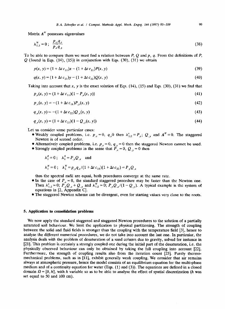
Fig. 1. Comparison between spectral radii: Case 1.

7.aIE-01

6.ooE-01 - N.- R.Stag.

5.ME-O1

4.0JE-01

3.COE-01

2.CQE-01

O.ooE+OO

1 6 20 70 300 8Ou 4000 QXO 14cca 19coO 24Oa

Ime @ed

Fig. 2. Comparison between spectral radii: Case 2.

35

--.--’ N.-R.Stan.

---- sw.suw.stag.

- N. -R. stacl.

5 t

04

1 6 20 70 3cn eal 4ooo wxx) 14lX0 19Wl 24cal

Ime Met)

Fig. 3. Comparison between number of iterations per time step in different solution procedures: Case 1

B.A. Schrejkr et al. I Comput. Methods Appl. Mech. Engrg. 144 (1997) 93-109 101

xl --

1! i 40--

3 30 --

% __ 2”

10 __ f

-----’ N.-R.Stan.

---- suc.subst.stag.

- N.- R Stag.

-----__-..-’

01 I

1 6 20 70 303 800 4ax Km 14CKO 19fYXl 24oml

lime (see)

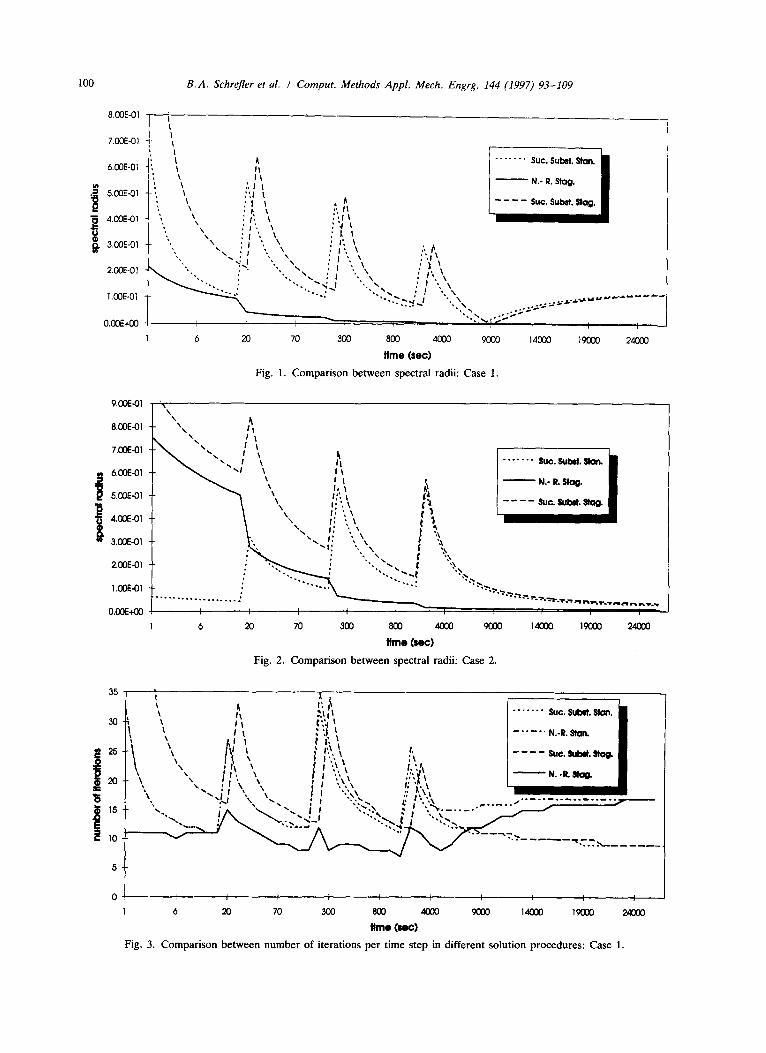
Fig. 4. Comparison between number of iterations per time step in different solution procedures: Case 2.

3.COE-02

2.5OE-02

! 2’00E-02 3 1.5OE-02

i l.DlE-02

5.oOE-03

O.COE+M)

..---.. succ.subst.stan.

- - - - succ. sub& stag.

----“‘N.-R.Stan.

- N.- R. Stag.

6 20 70 3al 800 4am woo 14Wl 19KO 24Krl

tlme (SW)

Fig. 5. Maximum error at the beginning of each time step: Case 1.

1.4OE-02 I I

1.2OE-02

l.KW2

‘0 8 8.C.QE-03 E

i

1 “mE-03 4.IXE-03

2.mE-03

O.WE+W

---- suc.suhlt.stag.

- -. -. N.- R. Stan.

- N.-R. Stag.

6 20 70 3al 800 4aYl m 14am 190x 24wO

time (ted Fig. 6. Maximum error at the beginning of each time step: Case 2.

102 B.A. Schrefler et al. I Cornput. Methods Appl. Mech. Engrg. 144 (1997) 93-109

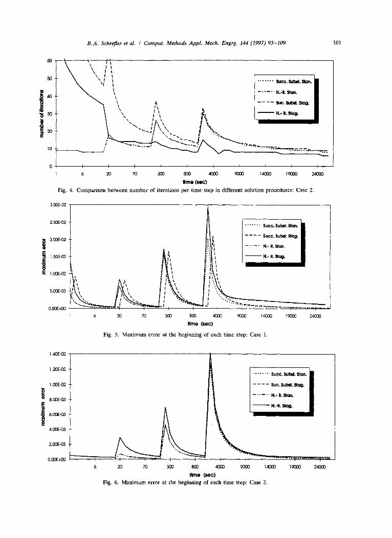
The test consists in solving a 1-D model problem with only 2 degrees of freedom. Dirichlet’s boundary conditions at x = h are associated with zero values of variables, while at h = 0 natural boundary conditions with zero force and flow are assigned. The forcing function is the gravitational effect on the liquid phase. Linear elastic behaviour is considered for the skeleton, while for water the non-linear relationships between capillary pressure, saturation and relative permeability proposed by Safai and Pinder [24] are considered. Spatial discretization is obtained by a single finite element with linear approximation for the field variables and the discretized system is obtained in a standard way

0 N.-R. Stag.

--_ n N.-R Stan I

SUC. Subst. Wm.

5 number d iterations

6y N.-R. Stag.

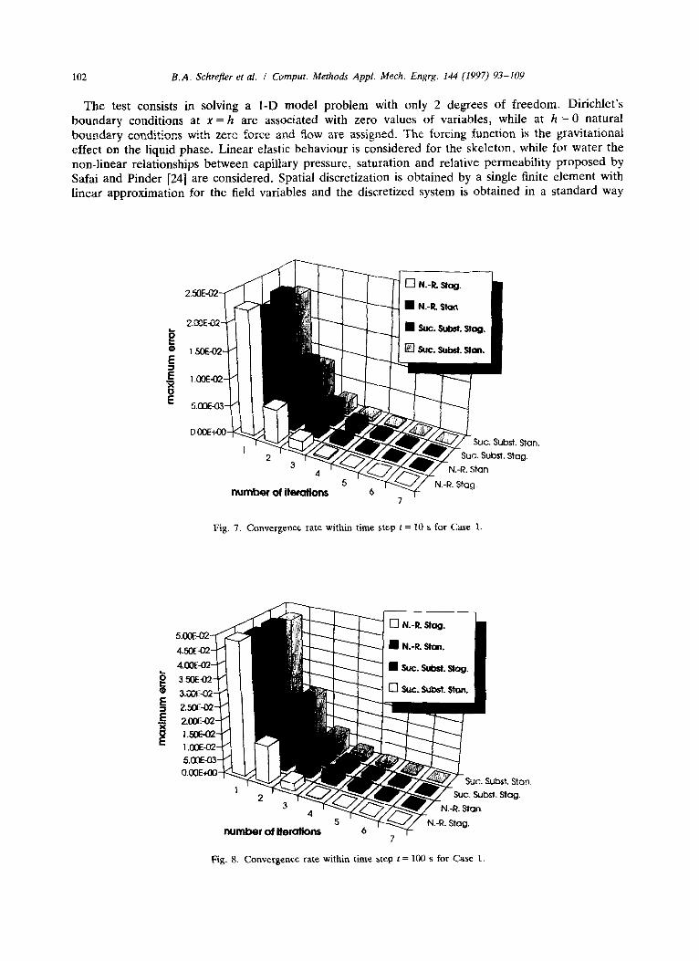
Fig. 7. Convergeoe rate within time step t = 10 s for Case 1.

number of iterdions

Fig. 8. Convergence rate within time step 1= 100 s for Case I.

xt. Stan. Stag.

B.A. Schrefler et al. I Comput. Methods Appl. Mech. Engrg. 144 (1997) 93-109 103

SW. Subst. Stan.

number ot iterations 7

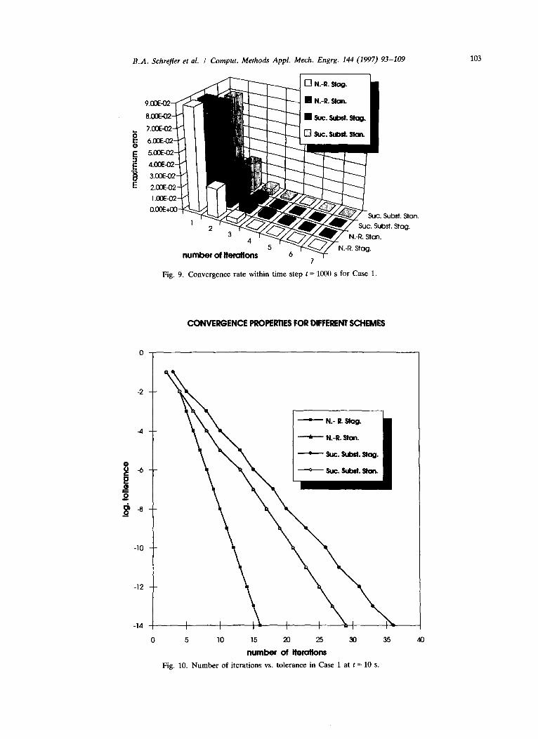
Fig. 9. Convergence rate within time step t = 1000 s for Case 1.

0

-2

-4

0 2 -6 E = e”

B -8

-10

-12

-14

CONVERGENCE PROPERTIES FOR DIFFERENT SCHEMES

- N.- R SMQ.

- N.-R Stan.

- sue. slat. stag.

-SUC.S&St.StUL

0 5 10 15 20 25 xl 35 40

number ot iterations

Fig. 10. Number of iterations vs. tolerance in Case 1 at t = 10 s.

104 B.A. Schrefler et al. ! Comput. Methods Appl. Mech. Engrg. 144 (1997) 93-109

using Gauss-Legendre’s quadrature formulae with two points. The analysed time span covers 7 hours from the start of the outflow. The time step is 1 s, then it is multiplied by 10 after every 10 steps until 10 000 s. As indicated in the Introduction, such an increase of time step length is common in practice in simulation of thermo-hydro-mechanical problems. The material has Young’s modulus of 1300 kN/m, porosity of 0.30 and absolute permeability of 0.045 and 0.0045 cm/s. Case 1 deals with parameter h = 50 cm, absolute permeability 0.045 cm/s, whereas Case 2 presents h = 100 cm and permeability 0.0045 cm/s.

For this limited class of solutions the comparison for the staggered procedures is performed and, at the same time, standard Newton-Raphson and direct successive substitution are applied.

As a general comment, we stress the complexity of the response during the time transient. Figs. l-6 present spectral radii, number of iterations within each time step and maximum error at the beginning of each time step, respectively, for Cases 1 and 2. The response is quite intricate and complicated. The peaks in these Figures are a consequence of the sudden changes in the time step length. A constant time step, or a more gradual change would avoid these peaks, but that does not necessarily mean a decrease in spectral radius, as can be seen in Fig. 1 after 10 000 s. Further, in Case 2 a sudden increase of the time step length produces for the staggered Newton even a decrease of the spectral radius and an ensuing reduction of the number of iterations, see Figs. 2 and 4.

In general, a certain superiority of the staggered Newton method can be drawn: with increasing time the method becomes of second order in Case 1. Case 2 reveals however a drastic increment of the


0

-2

-4

g-6 6 is = e

$4

-10

-12

-14

- N.-R Stag.

- N.-R Stan.

- sue. s&St. stag.

- sue. subst. Stan.

0 5 10 15 20 25 30 35 40

number d iterations

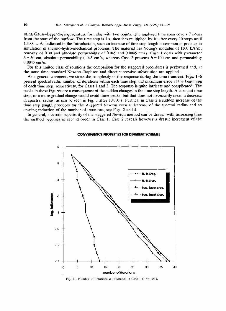
Fig. 11. Number of iterations vs. tolerance in Case 1 at t = 100 s.

B A. Schrefler et al. I Comput. Methods Appl. Mech. Engrg. 144 (1997) 93-109 105

spectral radius at the onset, hence general conclusions can hardly be made for both staggered procedures. Particular attention must be paid to limit of Eq. (35), especially for the first time steps.

We further point out the increase of the iteration number in Case 1 for t > 5000 s due to a larger maximum error at first iteration in each time step (Figs. 3 and 5). This suggests that the last solution used as predictor is less efficient in this algorithm. The dependence on the used material parameters of this fact is evidenced by Fig. 6, where the behaviour of the used predictor is the same for all procedures.

Figs. 7-9 present the drop in the initial error for the compared procedures at three time stations. They permit conclusions similar to those previously stated, also for the effect of the predictor.

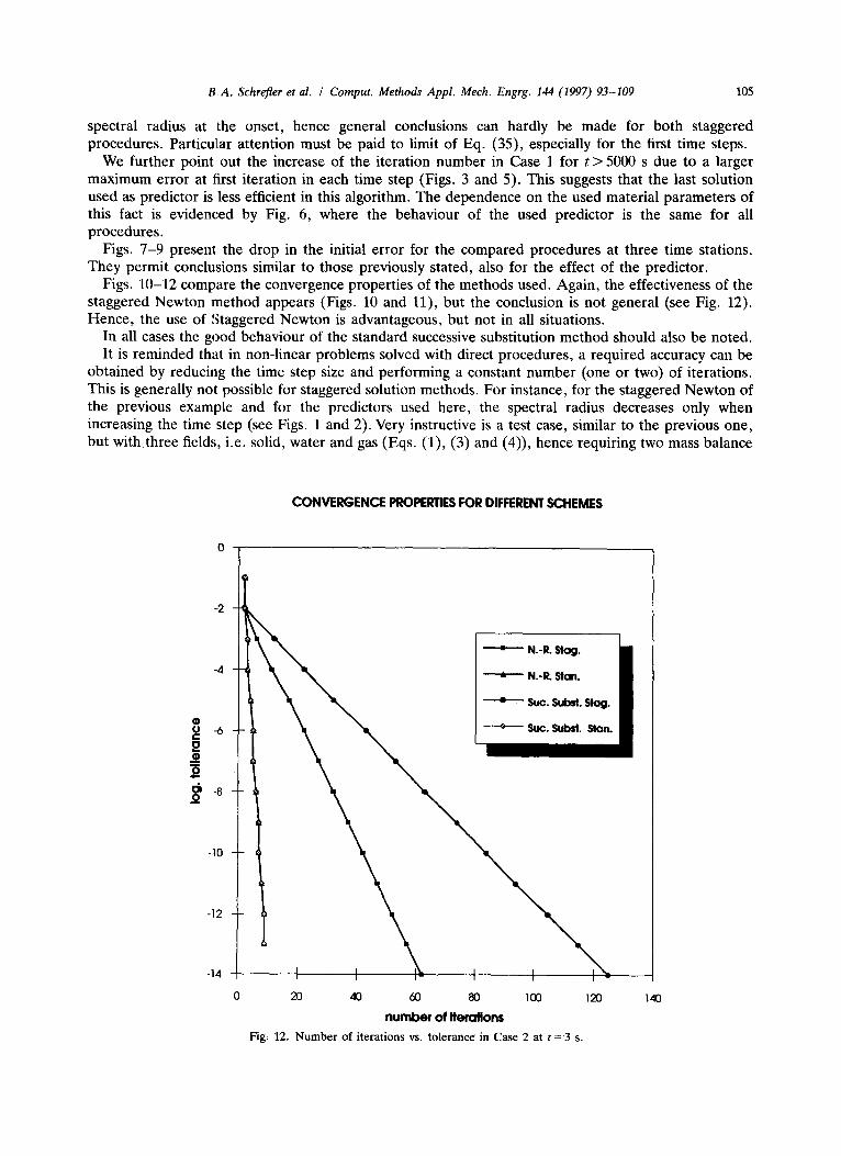
Figs. lo-12 compare the convergence properties of the methods used. Again, the effectiveness of the staggered Newton method appears (Figs. 10 and ll), but the conclusion is not general (see Fig. 12). Hence, the use of !Staggered Newton is advantageous, but not in all situations.

In all cases the good behaviour of the standard successive substitution method should also be noted. It is reminded that in non-linear problems solved with direct procedures, a required accuracy can be

obtained by reducing the time step size and performing a constant number (one or two) of iterations. This is generally not possible for staggered solution methods. For instance, for the staggered Newton of the previous example and for the predictors used here, the spectral radius decreases only when increasing the time step (see Figs. 1 and 2). Very instructive is a test case, similar to the previous one, but with,three fields, i.e. solid, water and gas (Eqs. (l), (3) and (4)), hence requiring two mass balance

0

-2

-4

8 -6 6 8 = e

g-8

-10

-12

-14


- N.-R. Stag.

--t- N.-R Stan.

- sue. !ilkbst. stag.

-suc.subst. Stan.

0 20 40 60 80 100 132

number of iterations Fig. 12. Number of iterations VS. tolerance in Case 2 at t = 3 s.


0.08

0.07 A A t=50 iter.

A A t=rO iter. o A t=tu non-iter.

n A t=50 non-iter.

m 0.06 a

5 0.05 m

t k 0.04

k m 3 0.03

tda 0 0.02

0.01

0, c?6 0 100 200 300 400 500 600

time (set)

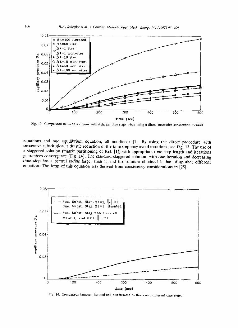
Fig. 13. Comparison between solutions with different time steps when using a direct successive substitution method.

equations and one equilibrium equation, all non-linear [l]. By using the direct procedure with successive substitution, a drastic reduction of the time step may avoid iterations, see Fig. 13. The use of a staggered solution (matrix partitioning of Ref. [l]) with appropriate time step length and iterations guarantees convergence (Fig. 14). The standard staggered solution, with one iteration and decreasing time step has a pectral radius larger than 1, and the solution obtained is that of another different equation. The form of this equation was derived from consistency considerations in [25].

d

enoa_

9 !

k 0.04-

i? a

z

4 0.02 -

time (set)

Fig. 14. Comparison between iterated and non-iterated methods with different time steps.

6. Conclusions

B.A. Schrefer et al. I Comput. Methods Appl. Mech. Engrg. 144 (1997) 93-109 107

Investigations of this paper have evidenced that there exists no definite conclusions about superior method for all non-linear situations.

The staggered Newton scheme demonstrates better convergence properties only for weakly coupled problems. Convergence of it requires restrictions imposed for Newton-Raphson method, the computa- tion of tangent matrices and condition (35) for convergence of iterations to be fulfilled. Thus, for strongly coupled problems the procedure is not so effective as expected. Similar conclusions can be drawn for the use of standard staggered procedures in strongly coupled problems: iteration convergence condition must be verified, not-only stability condition. Moreover, the influence of time step on convergence condition depends on the particular staggered solution used.

Acknowledgment

This research was meccanica numerica

Appendix A

partially supported by the MURST under the contract 40% 93B Algoritmi della non lineare su calcolatori ad architettura parallela.

The matrices appearing in Eqs. (6) are shown here in detail using the notation of [3]:


(WP)TAVNp df2 + I a NPT(p,C~S + pgC;ti)NP d0

F, = - n NPTph di2 + r NPT[q, - nT(pWC,wti + /+:ti)T] dT I I

where

+ np,Cz $! - nS,p,p,Cf 1

T + (1 - n)p,$ + nS,p,C,” + *S,p,C~

References

111

PI

[31

[41

[51

PI

[71

PI

[91

[lOI [Ill

(121

(131 [I41

L. Simoni and B.A. Schrefler, A staggered F.E. solution for water and gas flow in deforming porous media, Comm. Appl. Numer. Methods 7 (1991) 213-223. E. Turska and B.A. Schrefler, On convergence conditions of partitioned solution procedures for consolidation problems, Comput. Methods Appl. Mech. Engrg. 106(1-2) (1993) 51-64. R.W. Lewis and B.A. Schrefler, The Finite Element Method in the Deformation and Consolidation of Porous Media (J. Wiley & Sons, Chichester, 1987). O.C. Zienkiewics and A.H.C. Chart, Coupled problems and their numerical solution, in: J.St. Doltisnis, ed., Advances in Computational Nonlinear Mechanics (CISM Lecture Notes, Springer Verlag-Wien, 1989). K.C. Park, Stabilization of partitioned solution procedure for pore fluid-soil interaction analysis, Int. J. Numer. Methods Engrg. 19 (1983) 1669-1673. O.C. Zienkiewicz, D.K. Paul and A.H.C. Chan, Unconditionally stable staggered solution procedure for soil-pore fluid interaction problems, Int. J. Numer. Methods Engrg. 26 (1988) 1039-1055. K.C. Park, Partitioned transient analysis procedures for coupled-field problems: stability analysis, ASME J. Appl. Mech. 47 (1980) 370-376. K.C. Park and C.A. Felippa, Partitioned analysis of coupled systems, in: T. Belytschko and T.J.R. Hughes, eds., Computational Methods for Transient Analysis (Elsevier Science Publishers B.V., 1983). E. Turska, K. Wisniewski and B.A. Schrefler, Error propagation of staggered solution procedures for transient problems, Comput. Methods Appl. Mech. Engrg. 114 (1993) 51-63. G.F. Carey, Parallelism in finite element modelling, Comm. Appl. Numer. Methods 2(3) (1986) 281-288. F. Armero and J.C. Simo, A new unconditionally stable fractional step method for non-linear coupled thermo-mechanical problems, Int. J. Numer. Methods Engrg. 35 (1992) 737-766. N.N. Yanenko, Method of Fractional Steps for Solving Multi-Dimensional Problems of Mathematical Physics, Novosibirsk: Nauka (1967) [in Russian]. G.I. Marchuk, Methods of Numerical Analysis (Springer-Verlag, New York, 1975). A.J. Chorin et al., Product formulas and numerical algorithms, Comm. Pure Appl. Math. XXX1 (1978) 205-256.

[15] C. Miehe, Zur numerischen Behandlung thermomechanischer Prozesse, Forschungs- und Seminarberichte aus dem Bereich der Mechanik der Universtat Hannover, Bericht-Nr. F 88/6 (1988).

[16] G. Strang, Approximating semigroups and the consistency of difference methods, Proc. Am. Math. Sot. 20 (1969) 1-7. [17] C. Miehe, E. Stein and P. Wriggers, A general concept for thermomechanical coupling, in: S.N. Atluri and G. Yagawa, eds.,

Computational Mechanics 88, Proceedings of ICES Conference, Atlanta (Springer-Verlag, Berlin, 1988). [18] J.C. Simo and C. Miehe, Associative coupled thermoplasticity at finite strains: formulation, numerical analysis and

implementation, Comput. Methods Appl. Mech. Engrg. 98 (1992) 41-104. [19] P. Wriggers, C. Miehe, M. Kleiber and J.C. Simo, On the coupled thermomechanical treatment of necking problems via

finite element methods, Int. J. Numer. Methods Engrg. 33 (1993) 869-883. [20] D. Gawin, P. Baggio and B.A. Schrefler, Coupled heat, water and gas flow in deformable porous media, Int. J. Numer.

Methods Fluids 20 (1995) 969-987. [21] B.A. Schrefler and L. Simoni, A unified approach to the analysis of saturated-unsaturated elastoplastic porous media, in: G.

Swoboda, ed., Numerical Methods in Geomechanics, Innsbruck 1988 (Balkema, Rotterdam, 1988) 205-212. [22] T.N. Narashimhan and P.A. Witherspoon, Numerical model for saturated-unsaturated flow in deformable porous media. 3

Applications. Water Resour. Res. 14 (1978) 1017-1034.

B.,4. Schrejler et al. I Comput. Methods Appl. Mech. Engrg. 144 (1997) 93-109 109

[23] R.W. Lewis, B.A. Schrefler and L. Simoni, Coupling versus uncoupling in soil consolidation, Int. J. Numer. Methods Geomech. 15 (1991) 533-548.

[24] N.M. Safai and G.F. Pinder, Vertical and horizontal land deformation in a desaturating porous medium, Adv. Water Res. 2 (1979) 19-25.

[25] E. Turska and B.A. Schrefler, On consistency, stability and convergence of staggered solution procedures, Atti Act. Naz. Lincei, IX, V (1994) 265-271.