The impact of mobility networks on the worldwide
spread of epidemics
Alessandro Vespignani
Complex Systems GroupDepartment of InformaticsIndiana University
Complex Systems GroupDepartment of InformaticsIndiana University
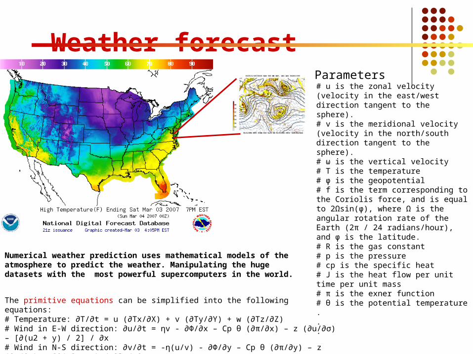
Weather forecast
The primitive equations can be simplified into the following equations:# Temperature: ∂T/∂t = u (∂Tx/∂X) + v (∂Ty/∂Y) + w (∂Tz/∂Z)# Wind in E-W direction: ∂u/∂t = ηv - ∂Φ/∂x – Cp θ (∂π/∂x) – z (∂u/∂σ) – [∂(u2 + y) / 2] / ∂x# Wind in N-S direction: ∂v/∂t = -η(u/v) - ∂Φ/∂y – Cp θ (∂π/∂y) – z (∂v/∂σ) – [∂(u2 + y) / 2] / ∂y# Precipitable water: ∂W/∂t = u (∂Wx/∂X) + v (∂Wy/∂Y) + z (∂Wz/∂Z)# Pressure Thickness: ∂(∂p/∂σ)/∂t = u [(∂p/∂σ)x /∂X] + v [(∂p/∂σ)y /∂Y] + z [(∂p/∂σ)z /∂Z]
# u is the zonal velocity (velocity in the east/west direction tangent to the sphere).# v is the meridional velocity (velocity in the north/south direction tangent to the sphere).# ω is the vertical velocity# T is the temperature# φ is the geopotential# f is the term corresponding to the Coriolis force, and is equal to 2Ωsin(φ), where Ω is the angular rotation rate of the Earth (2π / 24 radians/hour), and φ is the latitude.# R is the gas constant# p is the pressure# cp is the specific heat# J is the heat flow per unit time per unit mass# π is the exner function# θ is the potential temperature...
Parameters
Numerical weather prediction uses mathematical models of the atmosphere to predict the weather. Manipulating the huge datasets with the most powerful supercomputers in the world.
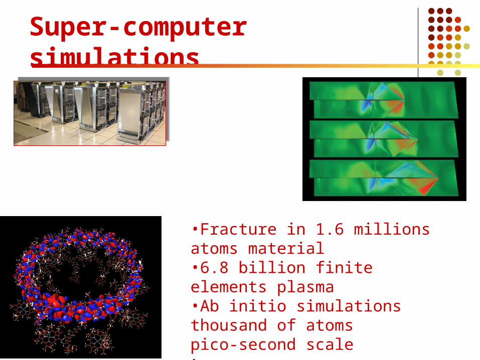
Super-computer simulations
•Fracture in 1.6 millions atoms material•6.8 billion finite elements plasma•Ab initio simulations thousand of atoms pico-second scale• ……
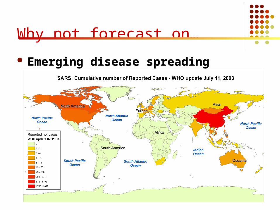
Why not forecast on…
Emerging disease spreading evolution
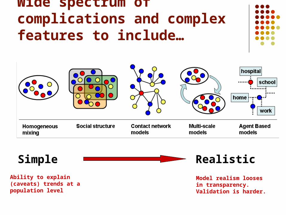
Wide spectrum of complications and complex features to include…
Simple Realistic
Ability to explain (caveats) trends at a population level
Model realism looses in transparency. Validation is harder.
Collective human behavior…. Social phenomena involves
large numbers of heterogeneous individuals over multiple time and size scales huge richness of cognitive/social science
In other words
The complete temperature analysis of the sea surface, and satellite images of atmospheric turbulence are easier to get than the large scale knowledge of commuting patterns or the quantitative measure of the propensity of a certain social behavior.
Unprecedented amount of data…..
Transportation infrastructures Behavioral Networks Census data Commuting/traveling patterns
Different scales: International Intra-nation (county/city/municipality) Intra-city (workplace/daily commuters/individuals behavior)
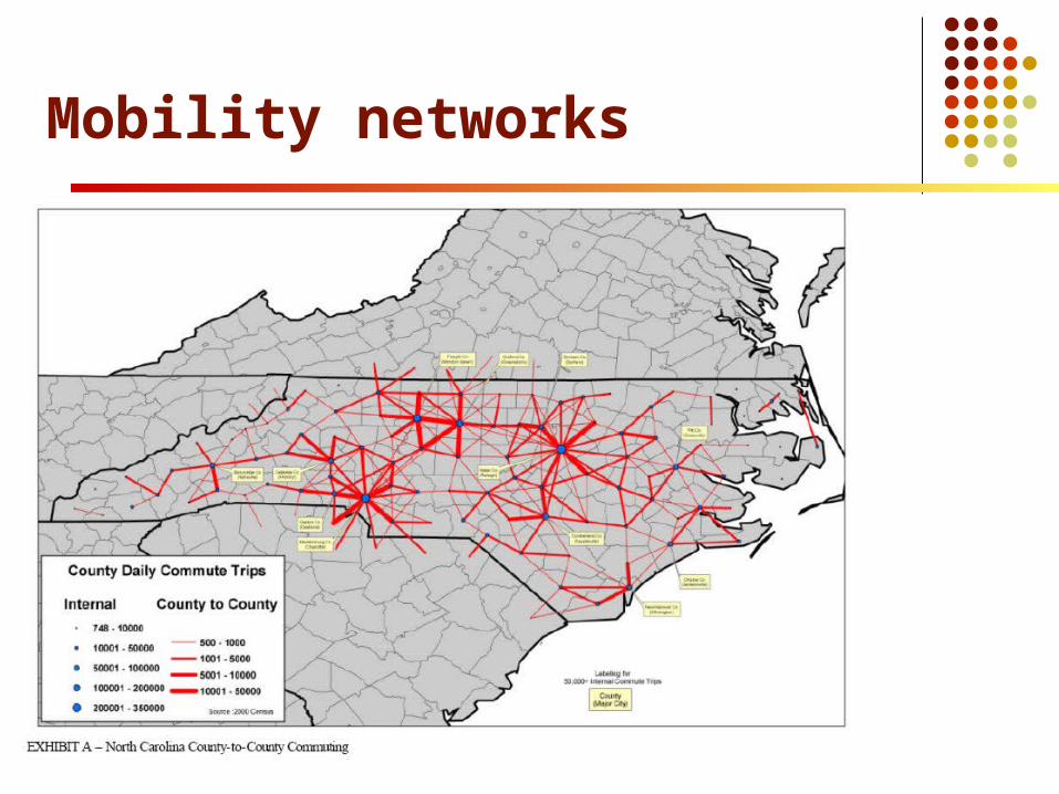
Mobility networks
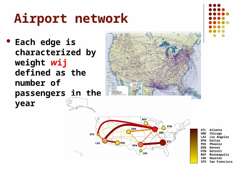
Airport network
Each edge is characterized by weight wij defined as the number of passengers in the year
LAX
ORD
ATL
DFW
SFO
DEN
PHX
DTW
IAH
MSP
ATL AtlantaORD ChicagoLAX Los AngelesDFW DallasPHX PhoenixDEN DenverDTW DetroitMSP MinneapolisIAH HoustonSFO San Francisco
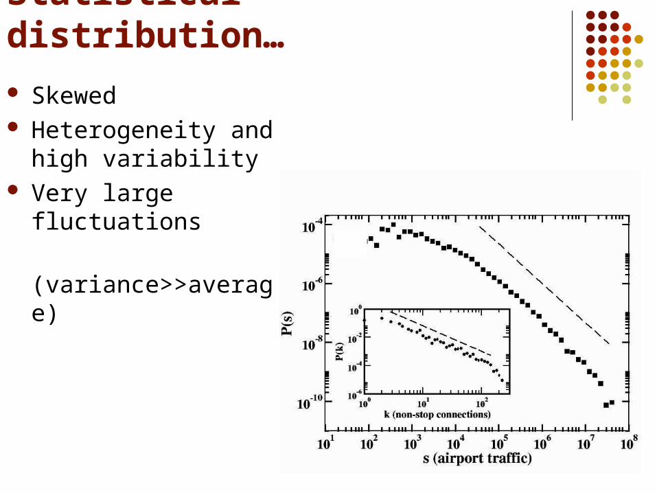
Statistical distribution…
Skewed Heterogeneity and high
variability Very large fluctuations
(variance>>average)
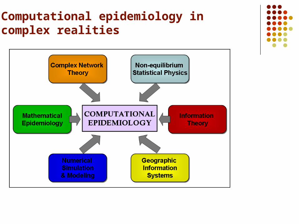
Computational epidemiology in complex realities
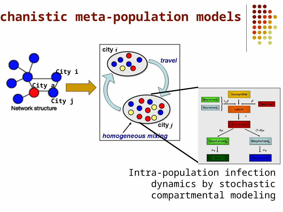
Mechanistic meta-population models
City a
City j
City i
Intra-population infection dynamics by stochastic compartmental
modeling
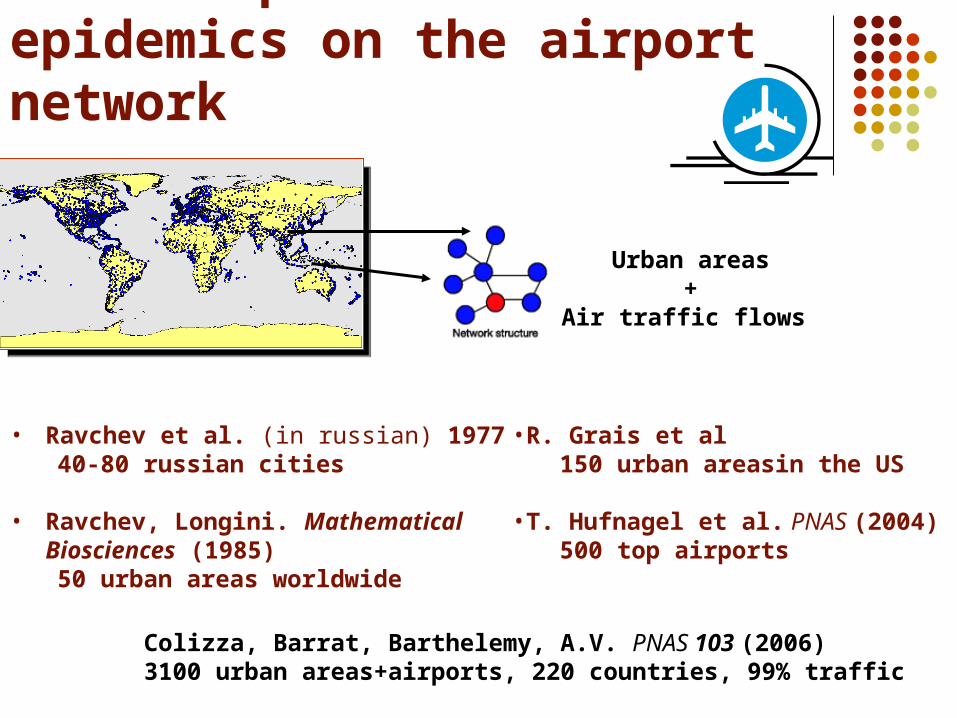
• Ravchev et al. (in russian) 197740-80 russian cities
• Ravchev, Longini. Mathematical Biosciences (1985)50 urban areas worldwide
Global spread of epidemics on the airport network
Urban areas+
Air traffic flows
•R. Grais et al 150 urban areasin the US
•T. Hufnagel et al. PNAS (2004)500 top airports
Colizza, Barrat, Barthelemy, A.V. PNAS 103 (2006)3100 urban areas+airports, 220 countries, 99% traffic
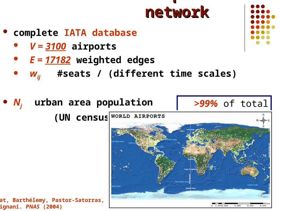
>99% of total traffic
Barrat, Barthélemy, Pastor-Satorras, Vespignani. PNAS (2004)
complete IATA database V = 3100 airports E = 17182 weighted edges wij #seats / (different time scales)
Nj urban area population
(UN census, …)
World-wide airport networkWorld-wide airport network
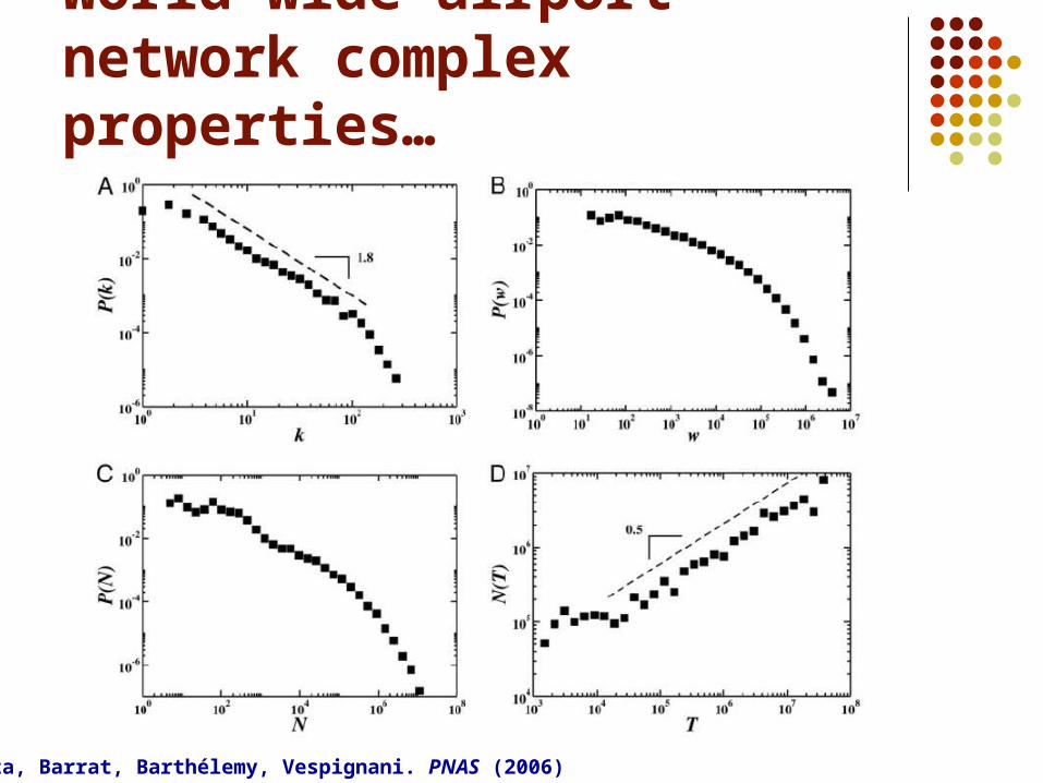
World-wide airport network complex properties…
Colizza, Barrat, Barthélemy, Vespignani. PNAS (2006)
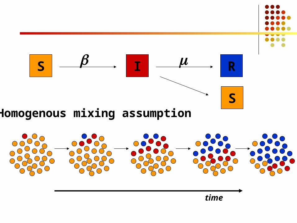
S I R
time
Homogenous mixing assumption
S
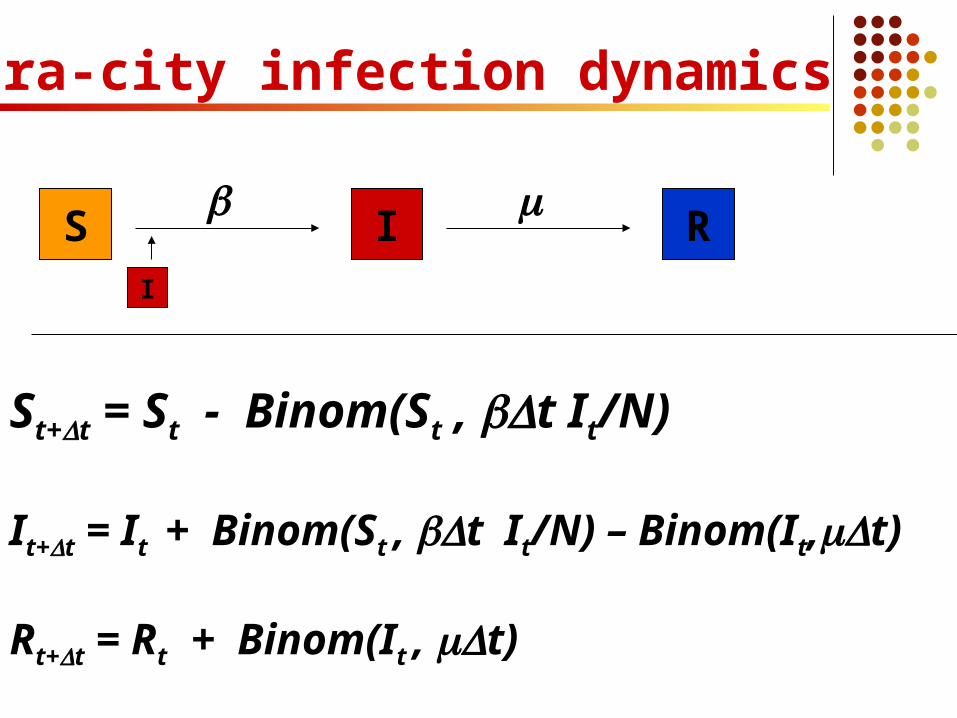
Intra-city infection dynamics
St+t = St - Binom(St , t It/N)
It+t = It + Binom(St , tIt/N) – Binom(It,t)
Rt+t = Rt + Binom(It , t)
S II
R
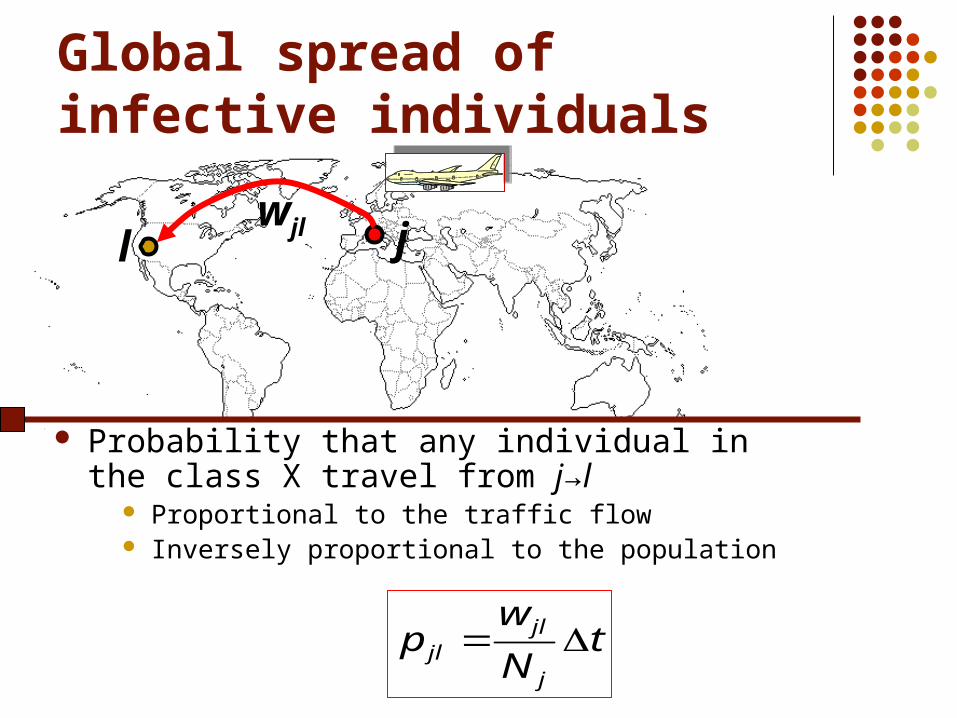
Global spread of infective individuals
jlwjl
tN
wp
j
jljl
Probability that any individual in the class X travel from j→l
Proportional to the traffic flow Inversely proportional to the population
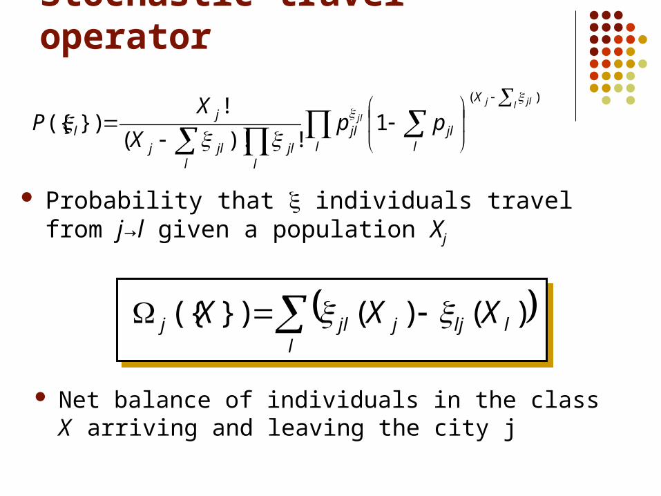
Stochastic travel operator
Probability that individuals travel from j→l given a population Xj
l
lljjjlj XXX )()(})({
l
X
ljljl
ljl
ljlj
jl
l jlj
jl ppX
XP
)(
1!)!(
!})({
Net balance of individuals in the class X arriving and leaving the city j
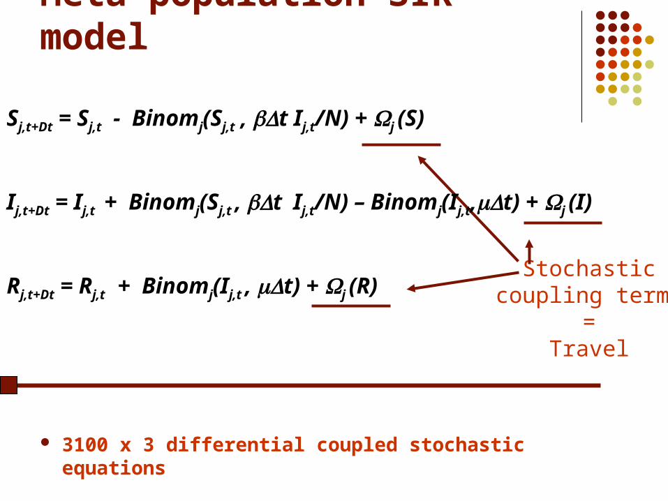
Meta-population SIR model
Stochasticcoupling terms
=Travel
3100 x 3 differential coupled stochastic equations
Sj,t+Dt = Sj,t - Binomj(Sj,t , t Ij,t/N) + j (S)
Ij,t+Dt = Ij,t + Binomj(Sj,t , tIj,t/N) – Binomj(Ij,t,t) + j (I)
Rj,t+Dt = Rj,t + Binomj(Ij,t , t) + j (R)

Directions…..
Basic theoretical questions…
Applications… Historical data Scenarios forecast
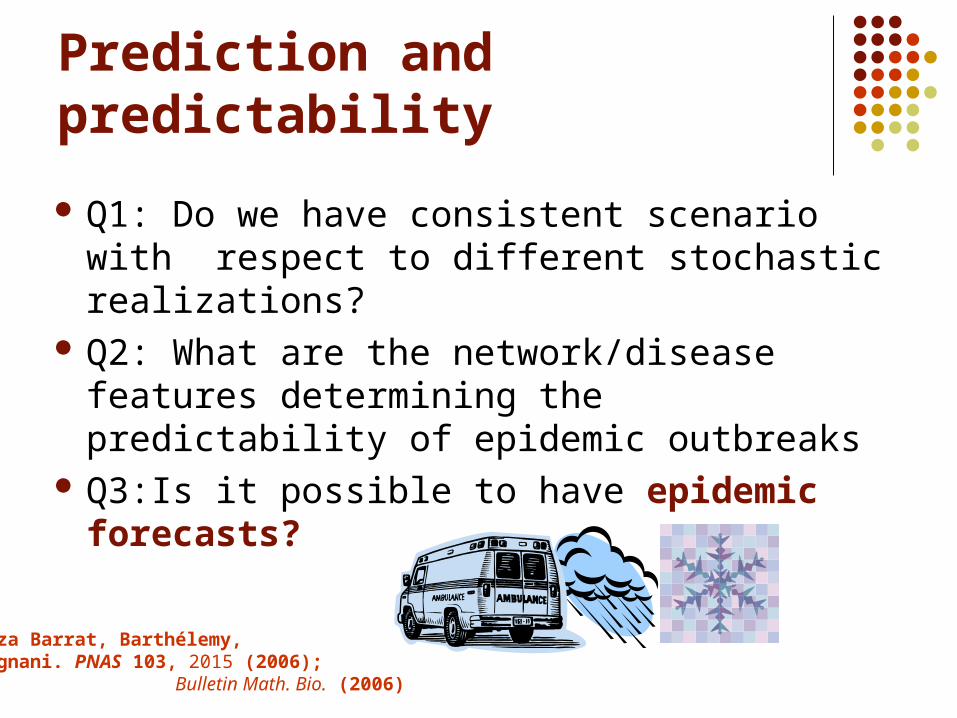
Prediction and predictability
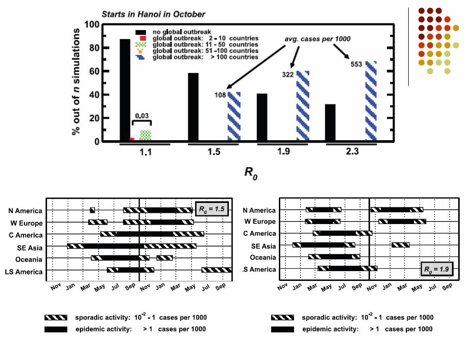
Q1: Do we have consistent scenario with respect to different stochastic realizations?
Q2: What are the network/disease features determining the predictability of epidemic outbreaks
Q3:Is it possible to have epidemic forecasts?
Colizza Barrat, Barthélemy, Vespignani. PNAS 103, 2015 (2006); Bulletin Math. Bio. (2006)
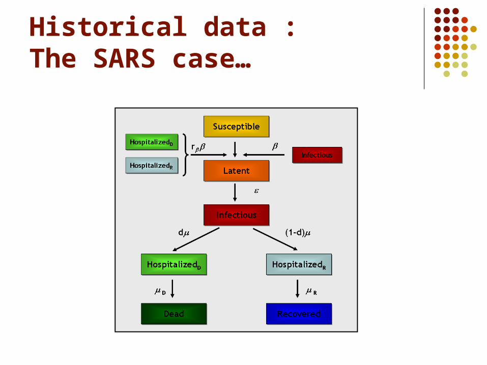
Historical data :The SARS case…
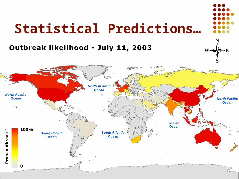
Statistical Predictions…
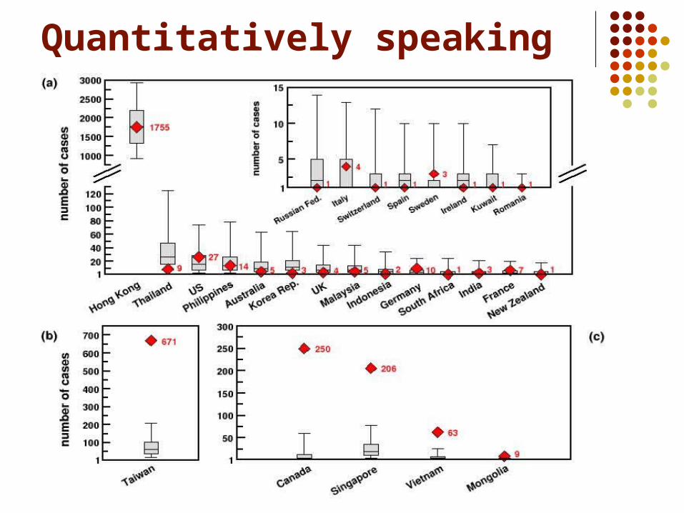
Quantitatively speaking
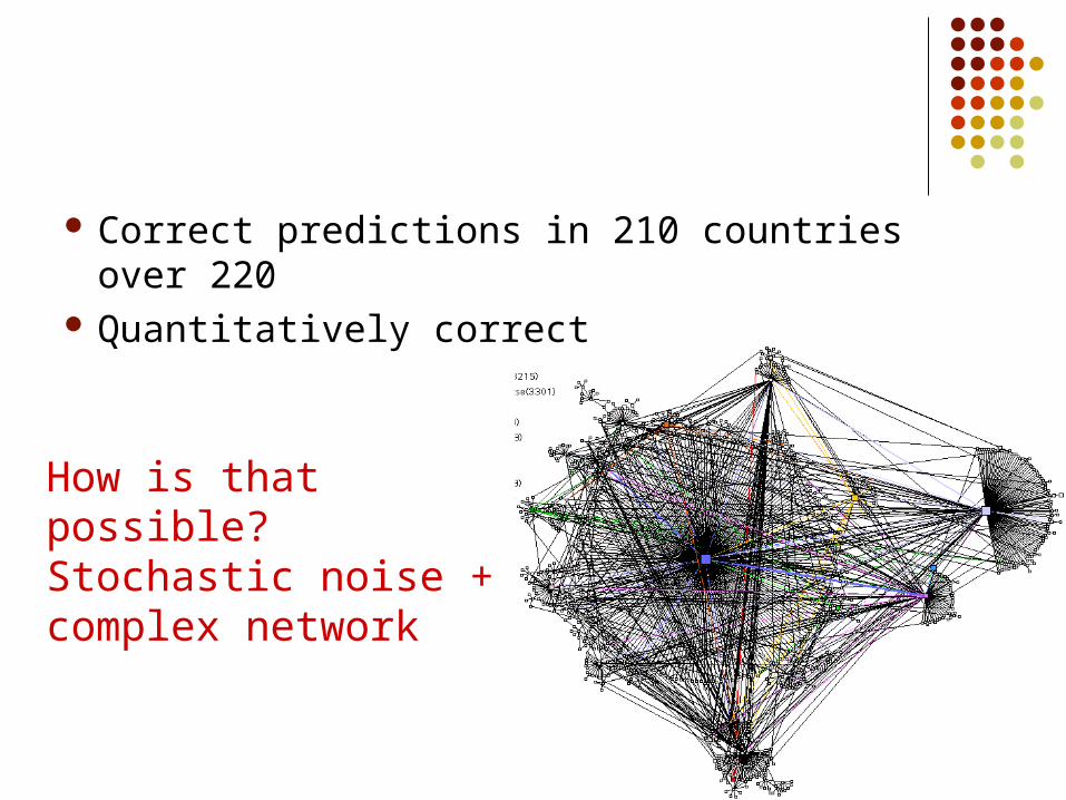
Correct predictions in 210 countries over 220 Quantitatively correct
How is that possible?Stochastic noise + complex network
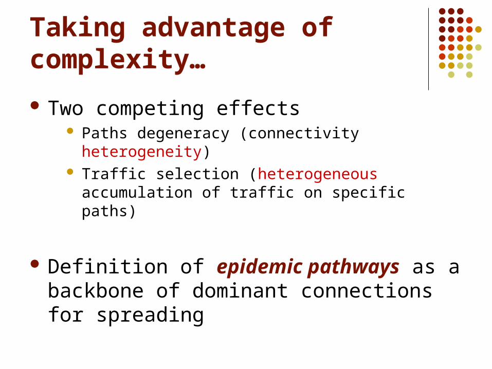
Taking advantage of complexity…
Two competing effects Paths degeneracy (connectivity heterogeneity) Traffic selection (heterogeneous accumulation of
traffic on specific paths)
Definition of epidemic pathways as a backbone of dominant connections for spreading
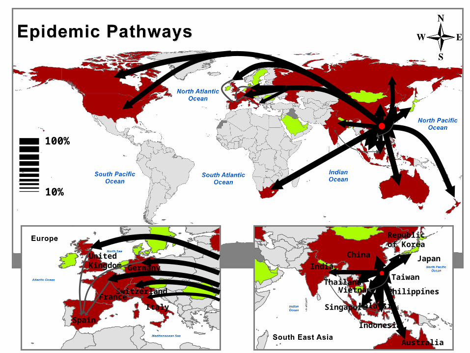
10%
100%
Germany
FranceItaly
Switzerland
United Kingdom
Spain
Australia
China JapanIndia
Indonesia
Malaysia
PhilippinesThailand
Vietnam
Republicof Korea
Taiwan
Singapore
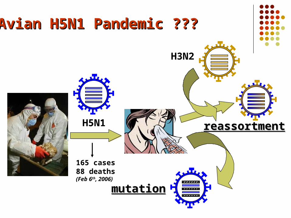
Avian H5N1 Pandemic ???Avian H5N1 Pandemic ???
H5N1
H3N2
reassortmentreassortment
mutationmutation
165 cases88 deaths(Feb 6th, 2006)
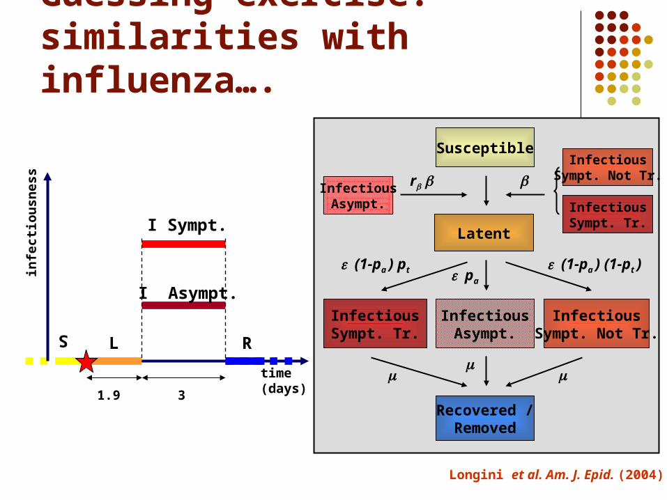
Recovered /Removed
InfectiousAsympt.
Latent
Susceptible
InfectiousSympt. Not Tr.
InfectiousSympt. Tr.
InfectiousAsympt. Infectious
Sympt. Tr.
InfectiousSympt. Not Tr.r
pa(1-pa ) pt (1-pa ) (1-pt )
time(days)
S
L R
I Sympt.
I Asympt.
1.9 3
Longini et al. Am. J. Epid. (2004)
infe
cti
ou
sn
ess
Guessing exercise: similarities with influenza….
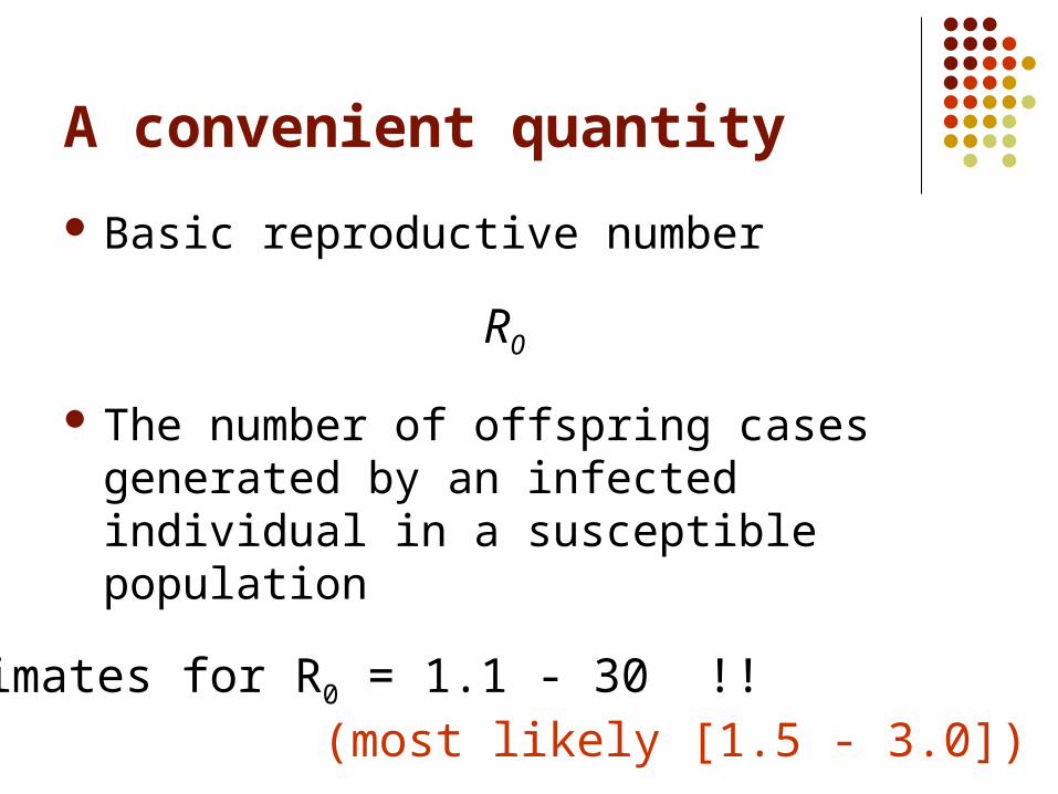
A convenient quantity
Basic reproductive number
The number of offspring cases generated by an infected individual in a susceptible population
R0
Estimates for R0 = 1.1 - 30 !!(most likely [1.5 - 3.0])
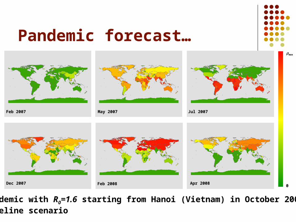
Feb 2007 May 2007 Jul 2007
Dec 2007 Feb 2008 Apr 20080
max
Pandemic with R0=1.6 starting from Hanoi (Vietnam) in October 2006Baseline scenario
Pandemic forecast…
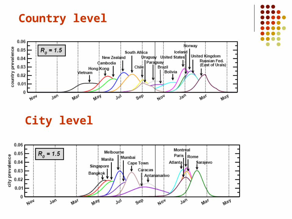
Country level
City level

Containment strategies…. Travel restrictions
Partial Full (country quarantine???)
Antiviral Amantadine and Rimantadine (inhibit matrix proteins) Zanamivir and Oseltamivir (neuraminidase inhibitor)
Vaccination Pre-vaccination to the present H5N1 Vaccine specific to the pandemic virus (6-9 months for
preparation and large scale deployment)
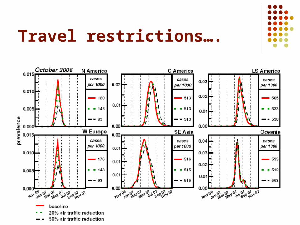
Travel restrictions….
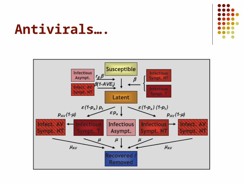
Antivirals….
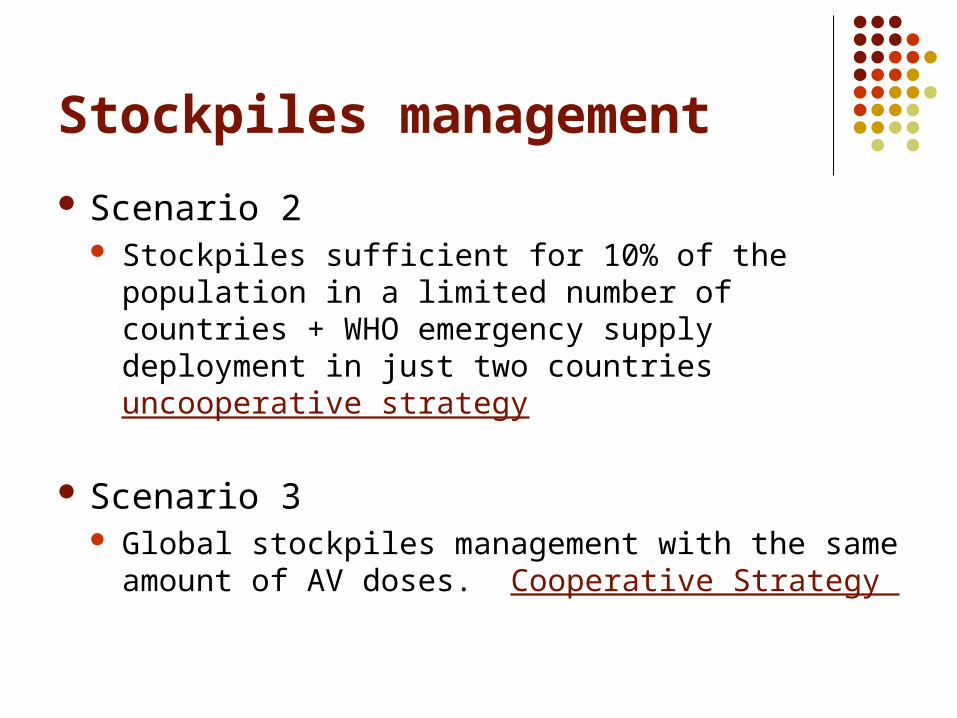
Stockpiles management
Scenario 2 Stockpiles sufficient for 10% of the population in a
limited number of countries + WHO emergency supply deployment in just two countries uncooperative strategy
Scenario 3 Global stockpiles management with the same
amount of AV doses. Cooperative Strategy
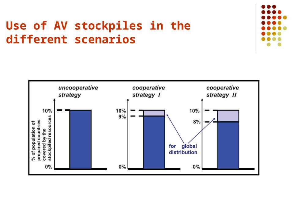
Use of AV stockpiles in the different scenarios
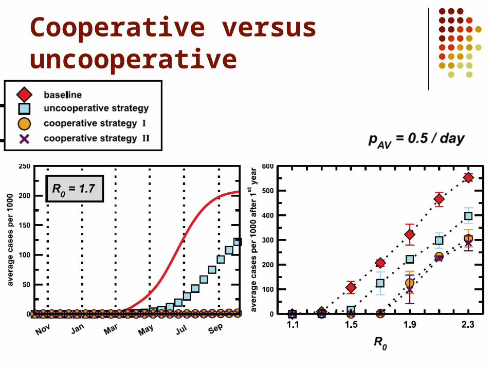
Cooperative versus uncooperative
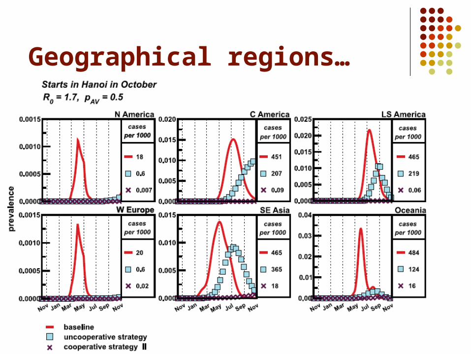
Geographical regions…
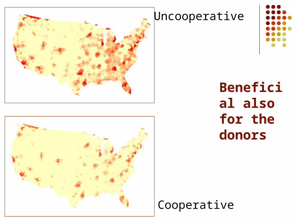
Beneficial also for the donors
Uncooperative
Cooperative
What we learn…
Complex global world calls for a non-local perspective
Preparedness is not just a local issue Real sharing of resources discussed by
policy makers …………
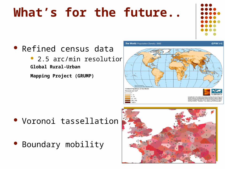
What’s for the future..
Refined census data 2.5 arc/min resolution Global Rural-Urban
Mapping Project (GRUMP)
Voronoi tassellation
Boundary mobility
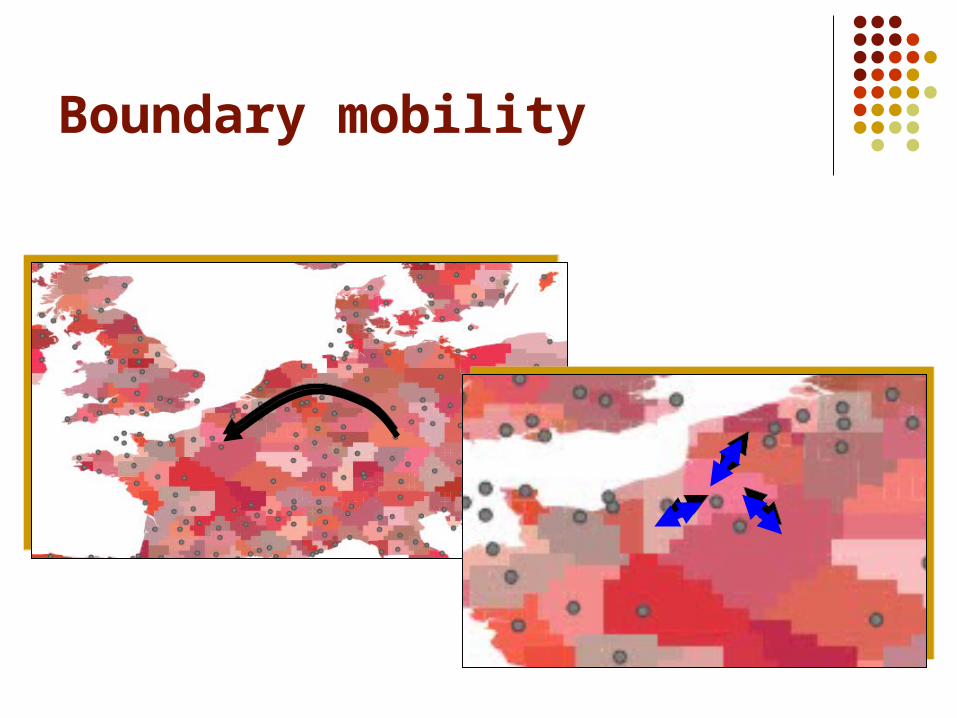
Boundary mobility
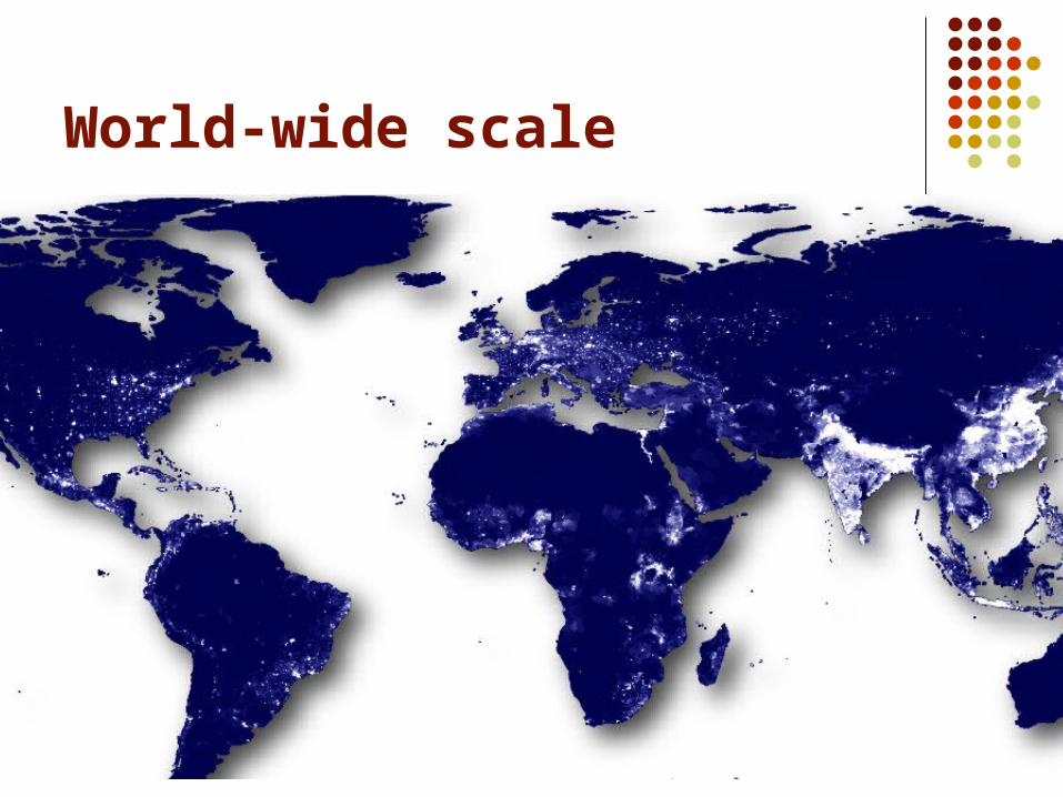
World-wide scale
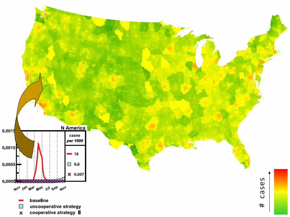
# ca
ses
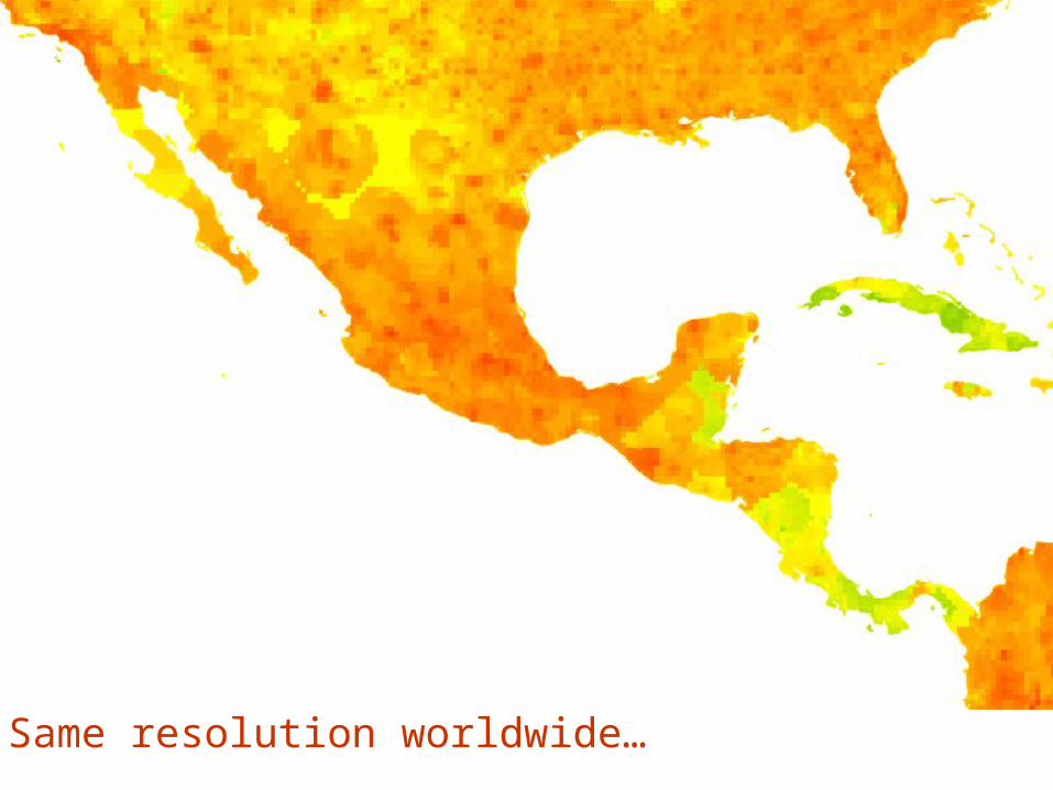
Same resolution worldwide…
Data integration + algorithms
Stochastic epidemic models Network models Data:
Census 3x10⁵ grid population IATA Mobility (US, Europe (12), Australia, Asia)
Visualization packages

Collaborators
V. Colizza A. Barrat
M. Barthelemy R. Pastor Satorras
More Information/paper/data
http://cxnets.googlepages.com
• A.J. Valleron
PNAS, 103, 2015-2020 (2006) Plos Medicine, 4, e13 (2007) Nature Physics, 3, 276-282 (2007)
Recommended