Valores Extremos Multivariados mediante R-vines
Leonardo Moreno
II Jornadas LPE-MAREN
La Paloma, Rocha, 2014

Esquema:
Eventos extremos
El Problema
Una idea de Copulas
Regular Vines
Estimacion y Predicciones

Eventos extremos climaticos.
Inundaciones rıo amarillo 1931China

Eventos extremos climaticos.
Inundaciones en LeonMexico

Eventos extremos climaticos.
Deslaves 1999Venezuela

Eventos extremos climaticos.
Temporal 2005Uruguay

Eventos extremos climaticos.
Temporal 2005Uruguay

Eventos extremos
¿Es posible predecir determinadoseventos extremos?

Poca informacion....
Figura : Estimacion de la cola de la distribucion

Una Aplicacion: LLuvias Extremas en Guanajuato
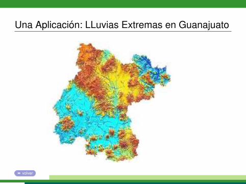
Una Aplicacion: LLuvias Extremas en Guanajuato
volver

Estaciones seleccionadas
●
●
●●
●
●
●
●
●
●
●
●
●
●
●
●
●
●
●
●
11001
11002
1100311005
11006
1100911013
11020
11021
11028
11031
11033
11036
11040
11051
11052
11071
11072
11079
11095
• Se decide trabajar con 20 estaciones que presentan datossimultaneamente en 37 anos.

Copulas: Teorema de Sklar
Para copulas bidimensionales
Sea H la funcion de distribucion conjunta de una v.a vectorial(X ,Y ) con F y G las distribuciones marginales (supongamoscontinuas). Entonces existe y es unica la copula C tal que∀(x , y) ∈ R
2cumple que,
H(x , y) = C(F (x),G(y)). (1)

Propiedades
• Sean M(u, v) ≡ min(u, v) y W (u, v) ≡ max(u + v − 1,0).Entonces para toda copula C se cumple que,
W (u, v) ≤ C(u, v) ≤ M(u, v). (2)
W y M son llamadas las cotas inferior y superior deFrechet-Hoeffding para Copulas
• Sean X e Y v.a absolutamente continuas. X e Y sonindependientes si y solo si CXY (u, v) = Π(u, v) ≡ u.v .

Densidad de la Funcion de Copula
Se llama densidad asociada a la copula C(u1,u2) a,
c(u1,u2) =∂2C(u1,u2)
∂u1∂u2. (3)
En v.a absolutamente continuas se cumple que,
f (x1, x2) = c(F1(x1),F2(x2))f1(x1)f2(x2), (4)

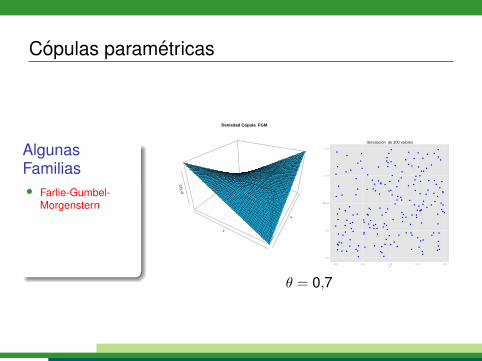
Copulas parametricas
AlgunasFamilias
• Farlie-Gumbel-Morgenstern
• Gaussiana
• Student
• Clayton

Copulas parametricas
AlgunasFamilias
• Farlie-Gumbel-Morgenstern
• Gaussiana
• Student
• Clayton
Copulas parametricas
AlgunasFamilias• Farlie-Gumbel-
Morgenstern
• Gaussiana
• Student
• Clayton
x
y
C(u,v)
Denisdad Cópula FGM
● ●
●
●
●
●
●
●
●
●
●
●
●
●
●
●
●
●
●
●
●
●
●
●
●
●
●
●
●
●
●
●
●
●
●
●
●
● ●
●
●
●
●
●
●
●
●
●
●
●
●
●
●
●
●
●
●
●
●
●
●
●
●
●
●
●
●
●
●
●
●
●
●
●
●
●
●
●
●
●
●
●
●
●
●
●
●
●
●
●●
●
●
●
●
●
●
●
●
●
●
●
●
●
●
● ●
●
●
●
●
●
●
●
● ●
●
●
●
●
●
●
●
●
●
●
●
●
●
●
●
●
●
●
●
●
●
●
●
●
●
●
●
●
●
●
●
●
●
●
●
●
●
●
●
●
●
●
●
●
●
●
●
●
●
●
●
●
●
●
●
●
●
●
●
●
●
●
●
●
●
●
●
●
●
●
●
●
●
●
●
●
●
●
●
●
●
●
●
●
0.00
0.25
0.50
0.75
1.00
0.00 0.25 0.50 0.75 1.00x
y
Simulación de 200 valores
θ = 0,7

Copulas parametricas
AlgunasFamilias• Farlie-Gumbel-
Morgenstern
• Gaussiana
• Student
• Clayton
x
y
C(u,v)
Densidad Cópula Normal
●
●
●
●
●
●
●
●
●
●
●
●
●
●
●
●●
●
●
●
●
●
●
●
●
●
●
●
●
●
●
●
●
●
●
●
●
●
●
●
●
●
●
●
●
●
●
●
●
●
●
●
●
●
●
●
●
●
●
●
●
●
●
●
●
●
●
●
●
●
●
●
●●
●
●
●
●
●
●
●
●
●
●
●
●
●
●
●
●●
●
●
●
●
●
●
●
●
●
●
●
●
●
●
●
●
●
●
●
●
●
●
●
●
●
●
●
●
●
●
●
●
●
●
●
●
●
●
●
●
●
●
●
●●
●
●
●
●
●
●
●
●
●
●
●
●
●
●
●
●
●
●
●
●
●
●
●
●
●
●
●
●
●
●
●
●●
●
●
●
●
●
●
●
●
●
●
●
●
●
●
●
●
●
●
●
●
●
●
●
●
●
●
●
●
●
●
●
0.00
0.25
0.50
0.75
1.00
0.00 0.25 0.50 0.75 1.00x
y
Simulación de 200 valores
θ = 0,25

Copulas parametricas
AlgunasFamilias• Farlie-Gumbel-
Morgenstern
• Gaussiana
• Student
• Clayton
x
y
C(u,v)
Densidad Cópula Student
●
●
●
●
●
●
●
●
●
●
●
●
●
●
●●
●
●
●
●
●
●
●
●
●
●
●
●
●
●
●
●
●
●
●
●
●
● ●
●
●
●
●
●
●
●
●
●
●
●
●●
●
●
●
●
●
●
●
●
●
●
●
●
●
●
●
●
●
●
●
●
●
●
●
●
●
●
●
●
●
●
●
●
●
●
●
●
●
●
●
●
●
●
●
●
●
●
●
●
●
●
●
●
●
●
●
●
●
●
●
●
●
●
●
●
●
●
●
●
●
●
●
●
●
●
●
●
●
●
●
●
●
●
●
●
●
●●
●
●
●
●
●
●
●
●
●
●
●
●
●
●
●
●
●
●
●
●
●
●
●
● ●
●
●
●
●
●
●
●
●
●
●
●
●
●
●
●
●
●
●
●
●
●
●
●
●
●
●
●
●
●
●
●
●
●
●
●
●
0.00
0.25
0.50
0.75
1.00
0.00 0.25 0.50 0.75 1.00x
y
Simulación de 200 valores
ρ = 0,7 y 4 g.l

Copulas parametricas
AlgunasFamilias• Farlie-Gumbel-
Morgenstern
• Gaussiana
• Student
• Clayton
x
y
C(u,v)
Densidad Cópula Clayton
●
●
●
●
●
●
●
●
●
●
●
●
●
●
●
●
●
●
●
●
●
●
●
●
●
●
●
●
●
●
●
●
●
●
●
●
●
●
●
●
●
●
●
●
●
●
●
●
●
●
●
●
●
●
●
●
●
●
●
●
●
●
●
●
●
●
●
●
●●●
● ●
●
●
●
●
●
●
●
●
●
●
●●
●
●
●
●
●
●
●●
●
●
●
●
●
●
●
●
●●
●
●
●
●
●
●
●
●
●
●
●
●
●
●
●
●
●
●
●
● ●
●
●
●
●
●
●
●
●
●
●
●
●
●
●
●
●
●
●
●
●
●
●
●
●
●
●
●
●
●
●
●
●
●
●
●
●
●
●
●
●
●
●
●
●
●
●
●
●
●
●
●
●
●
●
●
●●
●
●
●
●
●
●
●
●
●
●
●
●
●
●
●
●
●
●
●
0.00
0.25
0.50
0.75
1.00
0.00 0.25 0.50 0.75 1.00x
y
Simulación de 200 valores
θ = 1,5

Copulas Extremas
AlgunasFamilias
• Gumbel-Hougaard
• Galambos
• Husler-Reiss
• t-Extremal

Copulas Extremas
AlgunasFamilias
• Gumbel-Hougaard
• Galambos
• Husler-Reiss
• t-Extremal

Copulas Extremas
AlgunasFamilias• Gumbel-Hougaard
• Galambos
• Husler-Reiss
• t-Extremal
x
y
C(u,v)
Denisdad Cópula Gumbel
●
●
●
●
●
●
●
●
●
●
●
●
●
●
●
●
●
●
●
●
●
●
●
●
●
●
●
●
●
●●
●
●
●
●
●
●
●●
●
●
●
●
●
●
●
●
●
●
●
●
●
●
●
●
●
●
●
●
●
●
●
●
●
●
●
●
●
●
●
●
●
●
●
●
●
●
●
●
●
●
●
●
●
● ●
●
●
●
●
●
●
●
●
●
●
●
●
●
●
●
●
●
●
●
●
●
●
●
●
●
●
●
●●
●
●
●
●
●
●
●
●
●
●
●
●
●
●
●
●
●
●
●
●
●
●
●
●
●
●
●
●
●
●
●
●
●
●
●
● ●
●●
●
●
●
●
●
●
●
●
●
●
●
●
●
●
●
●
●●
●
●
●
●
●
●
●
●●
●
●
●
●
●
●
●
●
●
●
●
●
●
●
●
●
●
●
●
0.00
0.25
0.50
0.75
1.00
0.00 0.25 0.50 0.75 1.00x
y
Simulación de 200 valores
α = 2/3

Copulas Extremas
AlgunasFamilias• Gumbel-Hougaard
• Galambos
• Husler-Reiss
• t-Extremal
x
y
C(u,v)
Denisdad Cópula Galambos
●
●
●
●
●
●
●
●
●
●●
●
●
●
●
●
●
●
●
●
●
●
●
●
●
●
●
●
●
●
●
●
●
●
●
●
●
●
●
●
●
●
●
●
●
●
●
●
●
●
●
●
●
●
●
●
●
●
●
●
●
●
●
●
●
●
●
●
●
●
●
●
●
●
●
●
●
●
●●
●
●
●
●
●
●
●
●
●
●
●
●
●
●
●
●
●
●
●
●
●
●
●
●
●
●
●
●
●
●
●
●
●
● ●
●
●
●
●
●●
●
●●
●
●
●
●
●
●
●
●
●
●
●
●
●
●
●
●
●
●
●
●
●
●
●
●
●●
●
●
●
●
●
●
●
●
●
●
●
●
●
●
●
●
●
●
●
●
●
●
●
●
●
●
●
●
●●
●
●
●
●
●
●
●
●
●
●
●
●
●
●
●
●
●
● ●
●
0.00
0.25
0.50
0.75
1.00
0.00 0.25 0.50 0.75 1.00x
y
Simulación de 200 valores
α = 2/3

Copulas Extremas
AlgunasFamilias• Gumbel-Hougaard
• Galambos
• Husler-Reiss
• t-Extremal
x
y
C(u,v)
Densidad Cópula Husler−Reiss
●
●●
●
●
●●
●
●
●
●
●
●
●
●
●
●
●
●
●
●
●
●
●
●
●
●
●
●
●
●
●
●
●●
●
●
●
●
●
●
●
●
●
●
●
●
●
●
●
●
●
●
●●
●
●
●
●
●●
●
●
●
●
●
●
●
●
●
●
●
●
●
●
●
●
●
●
●
●
●
●
●
●
●
●
● ●
●
●
●
●
●
●
●
●
●
●
●
●
●
●
●
●
●
●
●
●
●
●
●
●
●
●
●
●
●
●
●
●
●
●
●
●
●
●
●
●
●
●
●
●
●
●
●
●
●
●
●
●
●
●
●
●
●
● ●
●
●
●
●
●
●
●
●
●
●
●
●
●
●
●
●
●
●
●
●
●
●
●
●
●
●
●
●
●
●
●
●
●
●
●
●
●
●
●
●
●
●
●
●
●
●
●
●
●
●
●
●
0.00
0.25
0.50
0.75
1.00
0.00 0.25 0.50 0.75 1.00x
y
Simulación de 200 valores
a = 3/2

Copulas Extremas
AlgunasFamilias• Gumbel-Hougaard
• Galambos
• Husler-Reiss
• t-Extremal
x
y
C(u,v)
Densidad Cópula t−extremal
●
●
●
●
●
●
●
●
●
●
●
●
●
●
●
●
●
●
●
●
●
●
●
●
●
●
●
●
●
●
●
●
●
●
●
●
●
●
●
●
●
●
●
●●
●
●
●
●
●
● ●
●
●
●
●
●
●
●
●
●
●
●
●
●
●●
●
●
●
●
●
●
●
●
●
●
●
●
●
●
●
●
●
●
●
●●
●
●
●
●
●
●
●
●
●
●
●
●
●
●
●
●●
●
●
●
●
●
●
●
●
●
●
●
●
●
●
●
●
●
●
●
●
●
●
●
●
●
●
●
●
●
●
●
●
●
●
●
●
●
●
●
●
●
●
●
●
●
●
●
●
●
●
●
●
●
●
●
●
●
● ●
●
●
●
●
●
●
●
●
●
●
●
●
●
●
●
●
●
●
●
●
●
●
●
●
●
●
●
●
●
●
●
●
●
●
●
●
0.00
0.25
0.50
0.75
1.00
0.00 0.25 0.50 0.75 1.00x
y
Simulación de 200 valores
ρ = 2/3 y 4 g.l

Estructura de R-vines
f1,2,3,4,5 = f1f2f3f4f5c12c13c34c15c23/1c14/3c35/1c24/13c45/13c25/134,
1
2
12
5
15
3
434
13
13
12
23/1
34
14/3
15
35/1
23/1 14/3 35/145/1324/13
24/13 45/1325/134
El numero posible de R-vines en Rd es d!2 2
(d−2)(d−3)2 .

Ejemplo. C-vines
f1,2,3,4,5 = f1f2f3f4f5c12c13c14c15c23/1c24/1c25/1c34/12c35/12c45/123
A1
1
2
12
3
13
4
14
5
15
A2
12
13
23/1
14
24/1
15
25/1
A3
23/1
24/1
34/1
2
25/135/12
A4
34/12
35/12
45/123

Ejemplos: D-vines
f1,2,3,4,5 = f1f2f3f4f5c12c23c34c45c13/2c24/3c35/4c14/23c25/34c15/234,
A1
1 2 3 4 545342312
A2
12 23 34 4535/424/313/2
A3
13/2 24/3 35/425/3414/23
A4
14/23 25/3415/234

Seleccion del Modelo
La seleccion de la copula R-vines consta de 3 pasos.
1. Seleccionar la estructura R-vines entre todas la posibles.2. Elegir las d(d − 1)/2 familias parametricas de copulas de a
pares.3. Estimar los parametros de las copulas seleccionadas.

Seleccion de la estructura R-vines
• Procedimiento secuencial introducido por Diımann,Brechmann, Czado y Kurowicka (2013), [5].
• Se elige una medida de dependencia δi,j que le asigne pesos alas aristas.
• Bajo un algoritmo (usamos Prim) adecuado se selecciona unarbol, el primero del conjunto, que maximice,∑
arsitas e={i,j}
|δi,j |

Relaciones de dependencia (δi ,j). Correlacion

Relaciones de dependencia. Correlacion
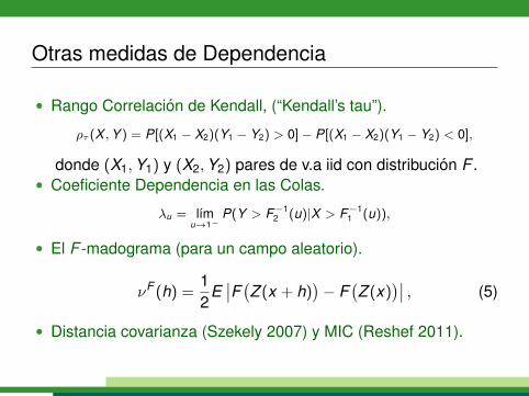
Otras medidas de Dependencia
• Rango Correlacion de Kendall, (“Kendall’s tau”).
ρτ (X ,Y ) = P[(X1 − X2)(Y1 − Y2) > 0]− P[(X1 − X2)(Y1 − Y2) < 0],
donde (X1,Y1) y (X2,Y2) pares de v.a iid con distribucion F .• Coeficiente Dependencia en las Colas.
λu = lımu→1−
P(Y > F−12 (u)|X > F−1
1 (u)),
• El F -madograma (para un campo aleatorio).
νF (h) =12
E∣∣F(Z (x + h)
)− F
(Z (x)
)∣∣ , (5)
• Distancia covarianza (Szekely 2007) y MIC (Reshef 2011).

Seleccion de Familias.
• Luego de elegida la estructura se seleccionan las familias decopulas bidimensionales y se estiman los parametros de cadacopula por maxima verosimilitud.
• El metodo de simplificacion, que consiste en considerarcopulas de una sola familia, y truncamiento, suponer que apartir de cierto nivel las copulas son independientes, fueronintroducidos por Brechmann, Czado y Aas en el 2012, [1].
• Por ultimo se calculan las distribuciones condicionalesempıricas de forma recursiva pues. A partir de ellas se reiterael algoritmo.

Primer arbol de la R-vine (lluvioso)
ver mapa
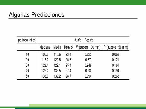
Algunas Predicciones
perıodo (anos) Junio − Agosto
Mediana Media Desvıo P∗(supere 100 mm) P∗(supere 150 mm)
10 105.2 110.6 23.4 0.625 0.06320 116.0 122.5 25.3 0.87 0.12130 123.4 129.1 25.4 0.948 0.16140 127.2 133.5 27.4 0.98 0.19450 133.0 139.2 28.7 0.994 0.268

GRACIAS!!

Referencias (1)
E.Brechmann; C. Czado; K. Aas.Truncated regular vines in high dimensions with application to financial data.Canadian Journal of Statistics, 40(1):68–85, 2012.
K. Aas; C. Czado; A. Frigessi; H. Bakken.Pair-copula constructions of multiple dependence.Insurance, Mathematics and Economics, 44:182–198, 2009.
J.F. Dissmann.Statistical inference for regular vines and application.Master’s thesis, Technische Universit at Munchen., 2010.
D. Kurowicka and R. Cooke.Uncertainty analysis with high dimensional dependence modelling.Wiley, 2006.
J. DiıMann; E. C. Brechmann; C. Czado; D. Kurowicka.Selecting and estimating regular vine copulae and application to financial returns.Computational Statistics & Data Analysis, 59:52–69, 2013.
O. Morales-Napoles.Bayesian belief nets and vines in aviation safety and other applications.PhD thesis, Technische Universiteit Delft, 2008.

Referencias (2)
R. Nelsen.An introduction to copulas.Springer-Verlag, 2006.
A. Sklar.Fonctions de repartition a n dimensions et leurs marges.Publ. Inst. Stat. Univ. Paris, 8:229–231, 1959.
R.M Cooke T. Bedford.Probability density decomposition for conditionally dependent random variables modeled by vines.Annals of Mathematics and Artificial Intelligence, 32:245–268, 2001.
H.Joe; J.J. Xu.The estimation method of inference functions for margins for multivariate models.Technical report, Department of Statistics, University of British Columbia, 1996.
Recommended