CCM – Valutazione Integrata di Impatto Ambientale e Sanitario
“Metodi per la valutazione integrata dell'impatto ambientale e sanitario (VIIAS)dell'inquinamento atmosferico”
Roma, 19 Aprile 2012
Prof. Fausto Manes
Dipartimento di Biologia Ambientale, Sapienza Università di Roma
Valutazione del verde urbano comepotenziale mitigatore dell’inquinamento
atmosferico
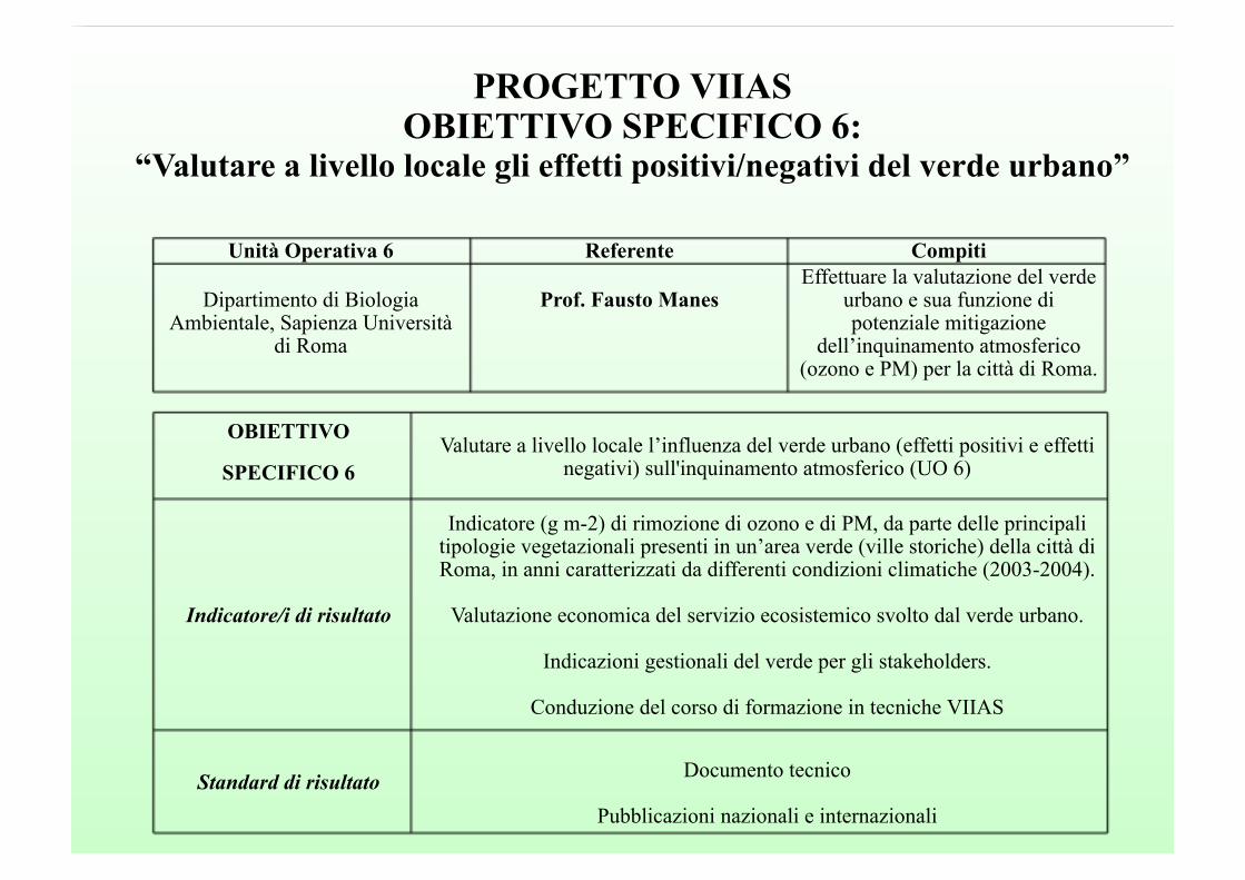
PROGETTO VIIASOBIETTIVO SPECIFICO 6:
“Valutare a livello locale gli effetti positivi/negativi del verde urbano”
Unità Operativa 6 Referente Compiti
Dipartimento di BiologiaAmbientale, Sapienza Università
di Roma
Prof. Fausto Manes
Effettuare la valutazione del verdeurbano e sua funzione dipotenziale mitigazione
dell’inquinamento atmosferico(ozono e PM) per la città di Roma.
OBIETTIVO
SPECIFICO 6Valutare a livello locale l’influenza del verde urbano (effetti positivi e effetti
negativi) sull'inquinamento atmosferico (UO 6)
Indicatore/i di risultato
Indicatore (g m-2) di rimozione di ozono e di PM, da parte delle principalitipologie vegetazionali presenti in un’area verde (ville storiche) della città diRoma, in anni caratterizzati da differenti condizioni climatiche (2003-2004).
Valutazione economica del servizio ecosistemico svolto dal verde urbano.
Indicazioni gestionali del verde per gli stakeholders.
Conduzione del corso di formazione in tecniche VIIAS
Standard di risultato
Documento tecnico
Pubblicazioni nazionali e internazionali
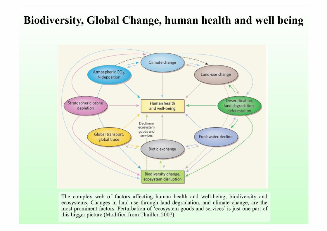
The complex web of factors affecting human health and well-being, biodiversity andecosystems. Changes in land use through land degradation, and climate change, are themost prominent factors. Perturbation of ‘ecosystem goods and services’ is just one part ofthis bigger picture (Modified from Thuiller, 2007).
Biodiversity, Global Change, human health and well being
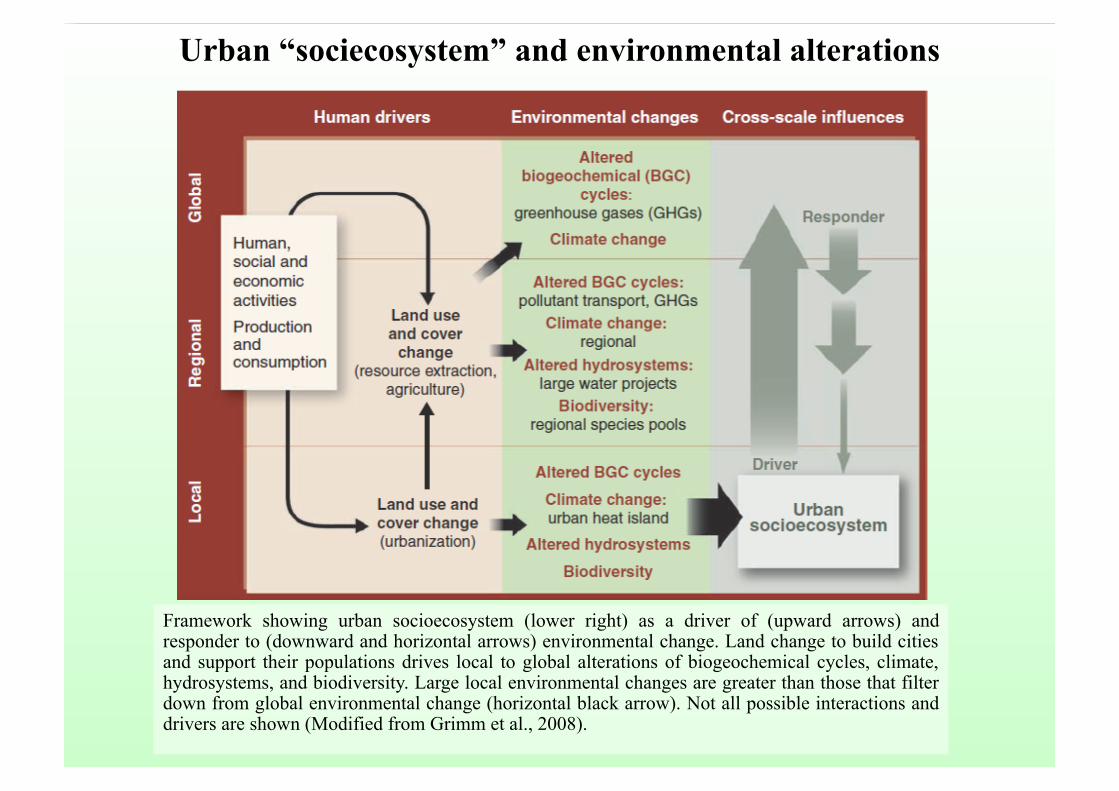
Urban “sociecosystem” and environmental alterations
Framework showing urban socioecosystem (lower right) as a driver of (upward arrows) andresponder to (downward and horizontal arrows) environmental change. Land change to build citiesand support their populations drives local to global alterations of biogeochemical cycles, climate,hydrosystems, and biodiversity. Large local environmental changes are greater than those that filterdown from global environmental change (horizontal black arrow). Not all possible interactions anddrivers are shown (Modified from Grimm et al., 2008).

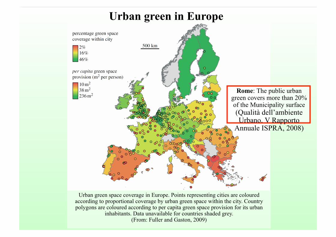
Urban green in Europe
Urban green space coverage in Europe. Points representing cities are colouredaccording to proportional coverage by urban green space within the city. Countrypolygons are coloured according to per capita green space provision for its urban
inhabitants. Data unavailable for countries shaded grey.(From: Fuller and Gaston, 2009)
Rome: The public urbangreen covers more than 20%of the Municipality surface(Qualità dell’ambienteUrbano. V Rapporto
Annuale ISPRA, 2008)
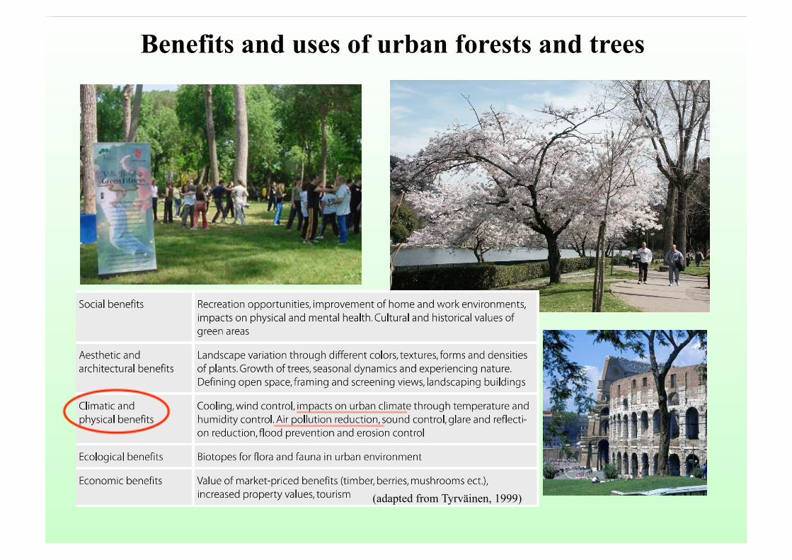
Benefits and uses of urban forests and trees
(adapted from Tyrväinen, 1999)
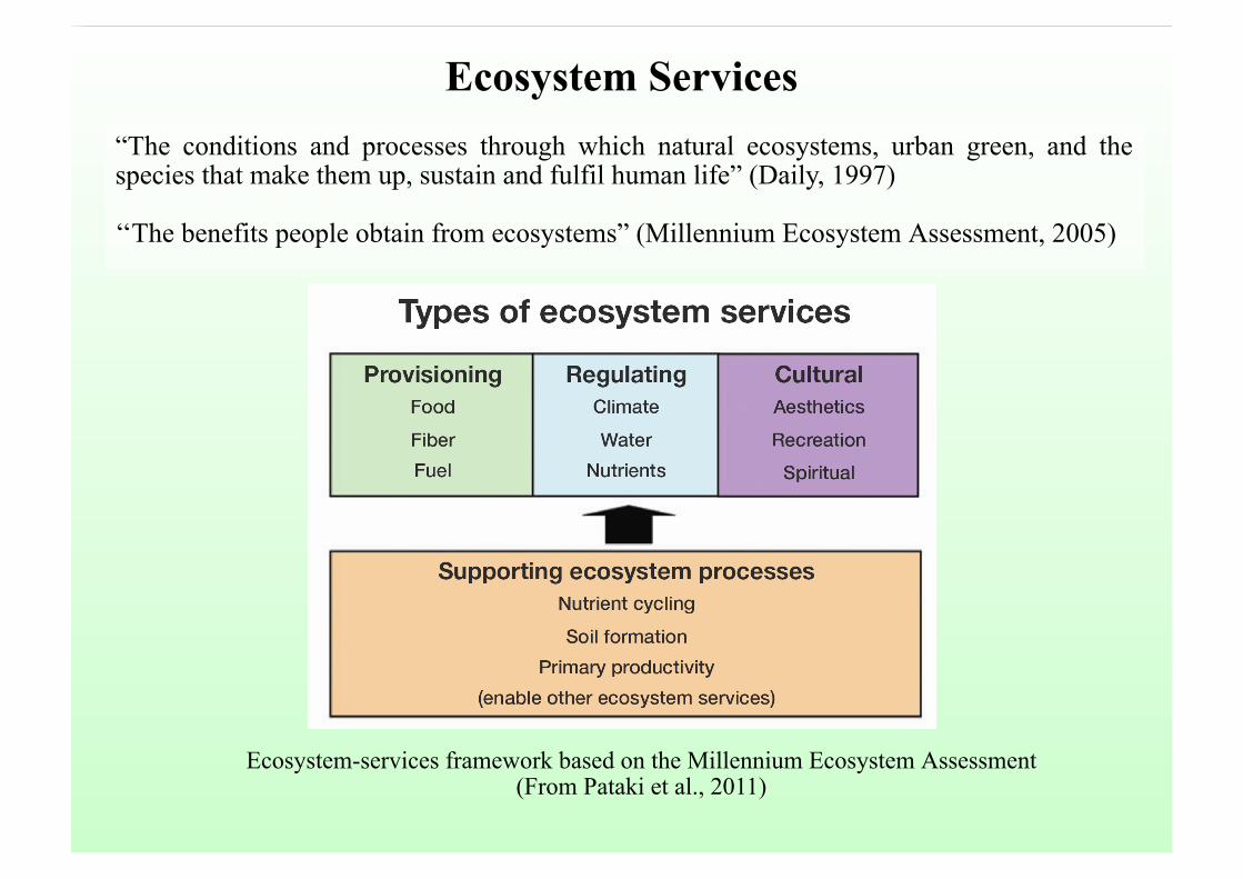
Ecosystem Services“The conditions and processes through which natural ecosystems, urban green, and thespecies that make them up, sustain and fulfil human life” (Daily, 1997) ‘‘The benefits people obtain from ecosystems” (Millennium Ecosystem Assessment, 2005)
Ecosystem-services framework based on the Millennium Ecosystem Assessment(From Pataki et al., 2011)
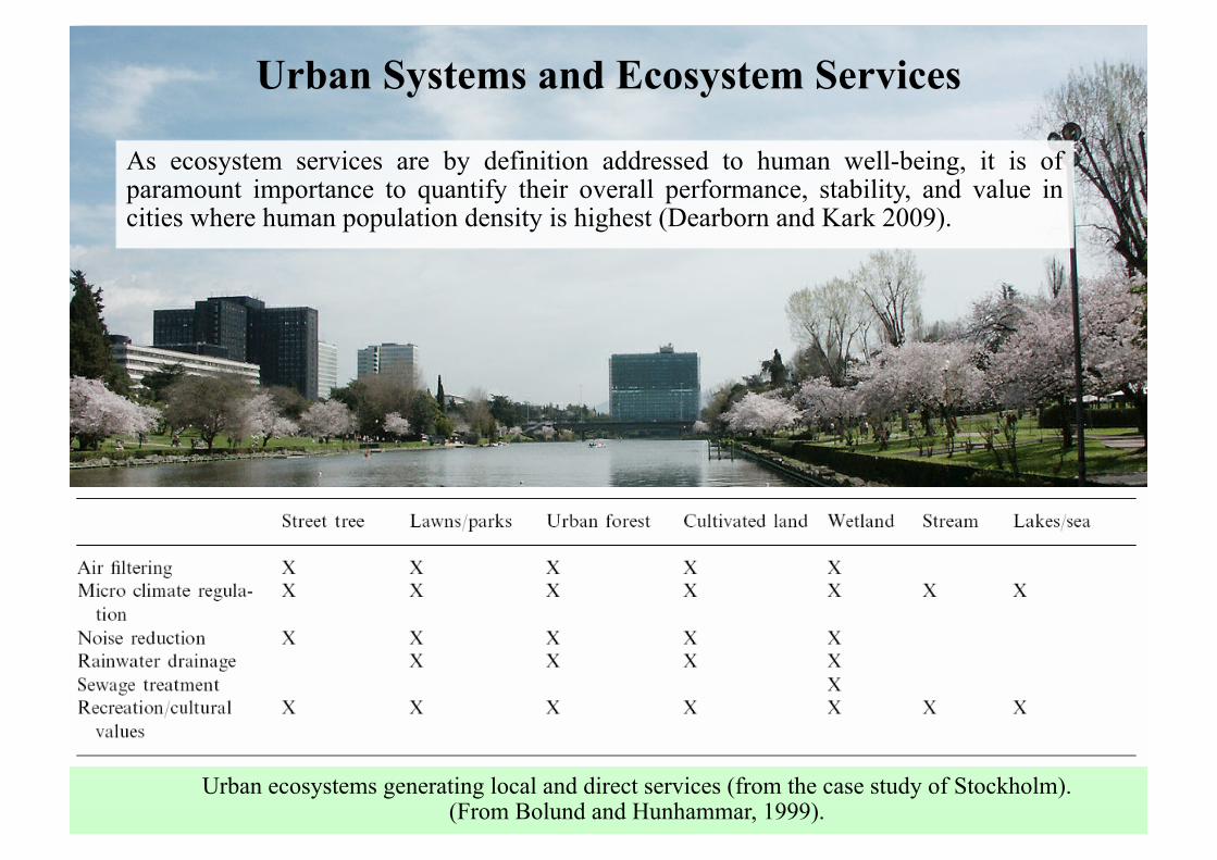
As ecosystem services are by definition addressed to human well-being, it is ofparamount importance to quantify their overall performance, stability, and value incities where human population density is highest (Dearborn and Kark 2009).
Urban Systems and Ecosystem Services
Urban ecosystems generating local and direct services (from the case study of Stockholm).(From Bolund and Hunhammar, 1999).
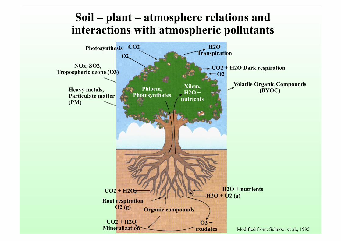
Soil – plant – atmosphere relations andinteractions with atmospheric pollutants
Heavy metals,Particulate matter(PM)
O2CO2Photosynthesis
NOx, SO2,Tropospheric ozone (O3)
H2OTranspiration
O2CO2 + H2O Dark respiration
Volatile Organic Compounds(BVOC)Phloem,
PhotosynthatesXilem,H2O +
nutrients
CO2 + H2O
Root respirationO2 (g) Organic compounds
H2O + nutrientsH2O + O2 (g)
O2 +exudates
CO2 + H2OMineralization Modified from: Schnoor et al., 1995
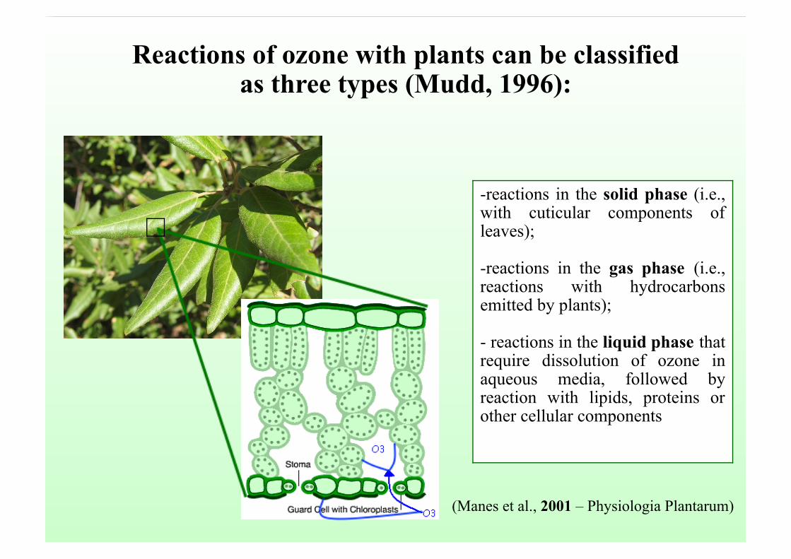
-reactions in the solid phase (i.e.,with cuticular components ofleaves); -reactions in the gas phase (i.e.,reactions with hydrocarbonsemitted by plants); - reactions in the liquid phase thatrequire dissolution of ozone inaqueous media, followed byreaction with lipids, proteins orother cellular components
Reactions of ozone with plants can be classifiedas three types (Mudd, 1996):
(Manes et al., 2001 – Physiologia Plantarum)
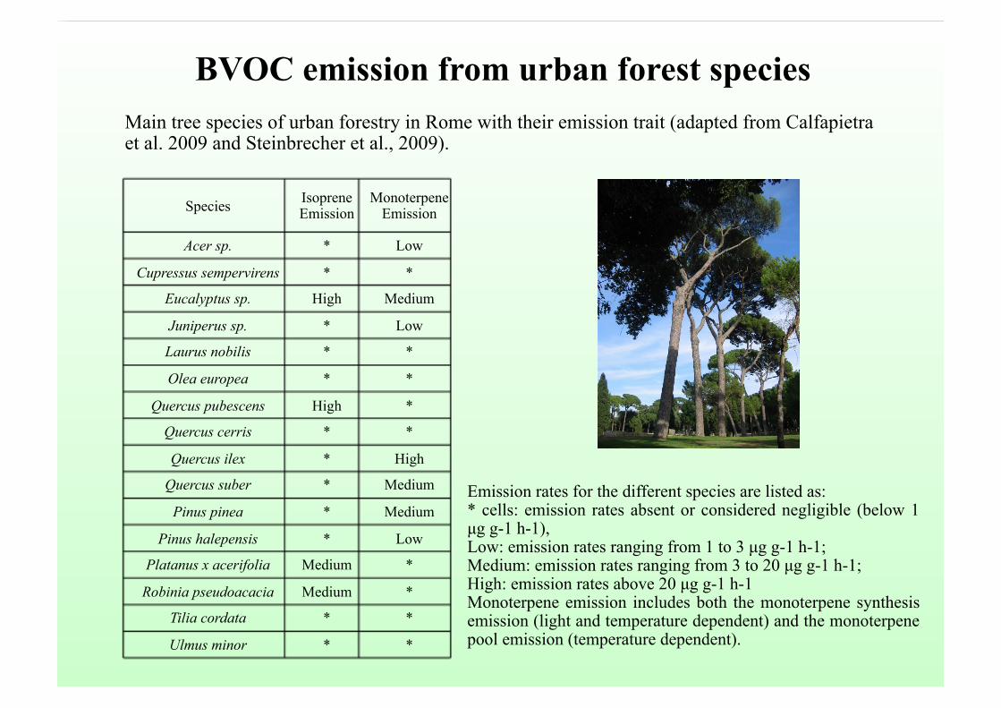
Species IsopreneEmission
MonoterpeneEmission
Acer sp. * Low
Cupressus sempervirens * *
Eucalyptus sp. High Medium
Juniperus sp. * Low
Laurus nobilis * *
Olea europea * *
Quercus pubescens High *
Quercus cerris * *
Quercus ilex * High
Quercus suber * Medium
Pinus pinea * Medium
Pinus halepensis * Low
Platanus x acerifolia Medium *
Robinia pseudoacacia Medium *
Tilia cordata * *
Ulmus minor * *
Emission rates for the different species are listed as:* cells: emission rates absent or considered negligible (below 1µg g-1 h-1),Low: emission rates ranging from 1 to 3 µg g-1 h-1;Medium: emission rates ranging from 3 to 20 µg g-1 h-1;High: emission rates above 20 µg g-1 h-1Monoterpene emission includes both the monoterpene synthesisemission (light and temperature dependent) and the monoterpenepool emission (temperature dependent).
Main tree species of urban forestry in Rome with their emission trait (adapted from Calfapietraet al. 2009 and Steinbrecher et al., 2009).
BVOC emission from urban forest species
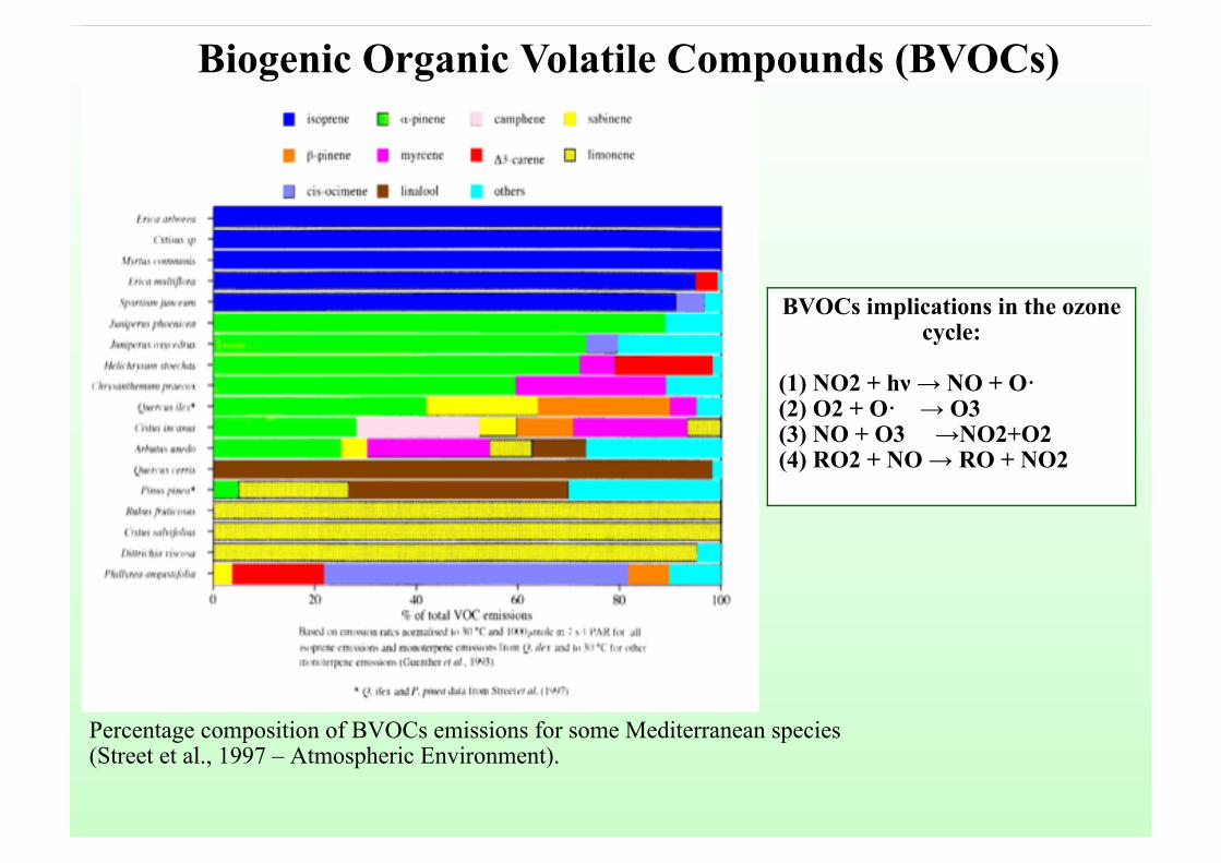
Percentage composition of BVOCs emissions for some Mediterranean species(Street et al., 1997 – Atmospheric Environment).
BVOCs implications in the ozonecycle:
(1) NO2 + hν → NO + O·(2) O2 + O· → O3(3) NO + O3 →NO2+O2(4) RO2 + NO → RO + NO2
Biogenic Organic Volatile Compounds (BVOCs)
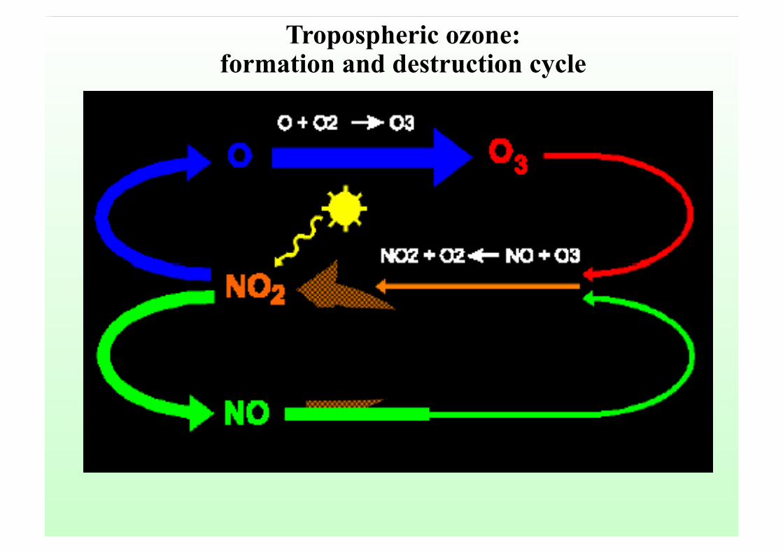
Tropospheric ozone:formation and destruction cycle
From: European Environmental Agency,Technical Report No 1/2009
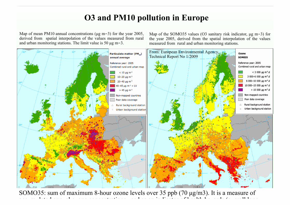
O3 and PM10 pollution in Europe
Map of mean PM10 annual concentrations (µg m-3) for the year 2005,derived from spatial interpolation of the values measured from ruraland urban monitoring stations. The limit value is 50 µg m-3.
Map of the SOMO35 values (O3 sanitary risk indicator, µg m-3) forthe year 2005, derived from the spatial interpolation of the valuesmeasured from rural and urban monitoring stations.
SOMO35: sum of maximum 8-hour ozone levels over 35 ppb (70 µg/m3). It is a measure ofaccumulated annual ozone concentrations used as an indicator of health hazards (overall long-
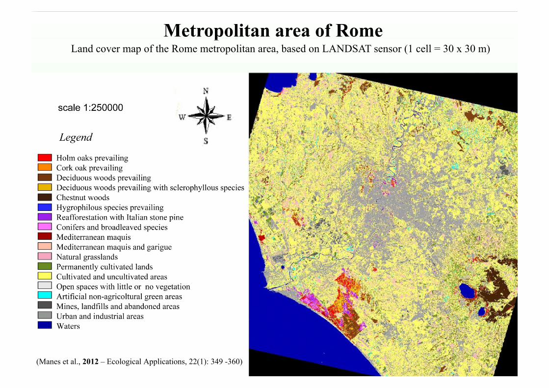
Metropolitan area of RomeLand cover map of the Rome metropolitan area, based on LANDSAT sensor (1 cell = 30 x 30 m)
(Manes et al., 2012 – Ecological Applications, 22(1): 349 -360)
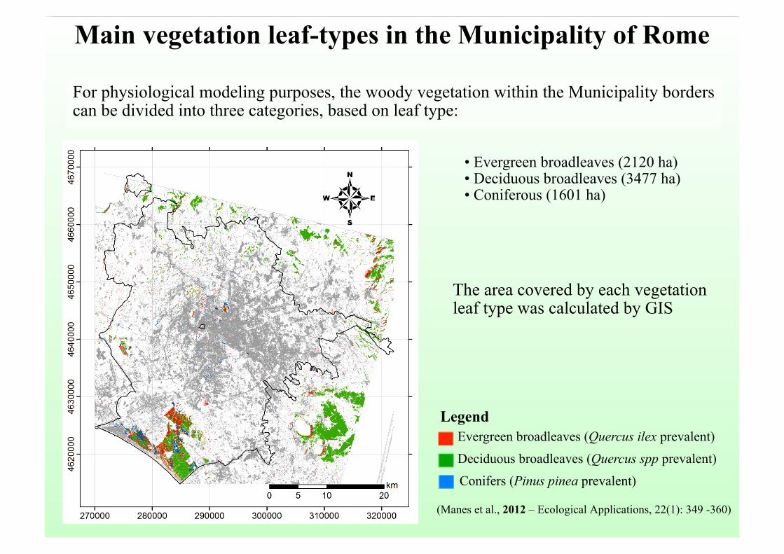
For physiological modeling purposes, the woody vegetation within the Municipality borderscan be divided into three categories, based on leaf type:
• Evergreen broadleaves (2120 ha)• Deciduous broadleaves (3477 ha)• Coniferous (1601 ha)
Main vegetation leaf-types in the Municipality of Rome
The area covered by each vegetationleaf type was calculated by GIS
Legend
Deciduous broadleaves (Quercus spp prevalent)
Evergreen broadleaves (Quercus ilex prevalent)
Conifers (Pinus pinea prevalent)
(Manes et al., 2012 – Ecological Applications, 22(1): 349 -360)
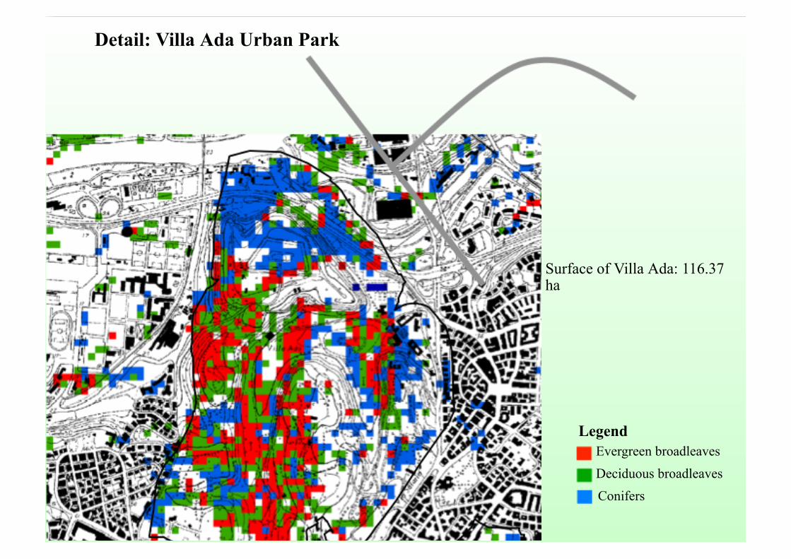
Detail: Villa Ada Urban Park
Legend
Deciduous broadleaves
Evergreen broadleaves
Conifers
Surface of Villa Ada: 116.37ha
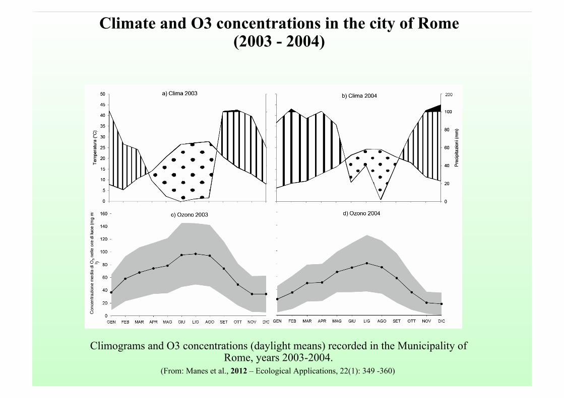
Climate and O3 concentrations in the city of Rome(2003 - 2004)
Climograms and O3 concentrations (daylight means) recorded in the Municipality ofRome, years 2003-2004.
(From: Manes et al., 2012 – Ecological Applications, 22(1): 349 -360)
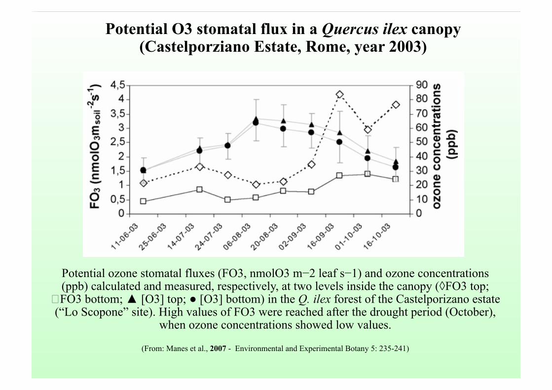
Potential ozone stomatal fluxes (FO3, nmolO3 m−2 leaf s−1) and ozone concentrations(ppb) calculated and measured, respectively, at two levels inside the canopy (◊FO3 top;
�FO3 bottom; ▲ [O3] top; ● [O3] bottom) in the Q. ilex forest of the Castelporizano estate(“Lo Scopone” site). High values of FO3 were reached after the drought period (October),
when ozone concentrations showed low values.
(From: Manes et al., 2007 - Environmental and Experimental Botany 5: 235-241)
Potential O3 stomatal flux in a Quercus ilex canopy(Castelporziano Estate, Rome, year 2003)
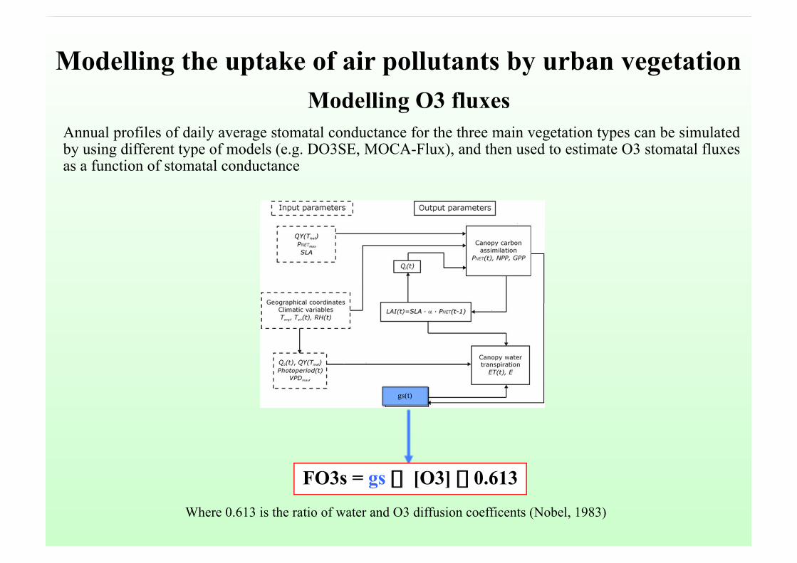
FO3s = gs �� [O3] �� 0.613
Where 0.613 is the ratio of water and O3 diffusion coefficents (Nobel, 1983)
Annual profiles of daily average stomatal conductance for the three main vegetation types can be simulatedby using different type of models (e.g. DO3SE, MOCA-Flux), and then used to estimate O3 stomatal fluxesas a function of stomatal conductance
Modelling the uptake of air pollutants by urban vegetation Modelling O3 fluxes
gs(t)
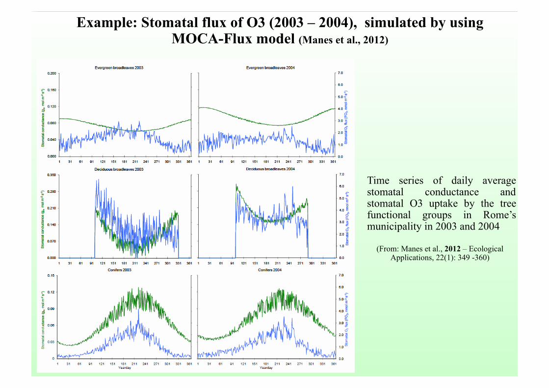
Time series of daily averagestomatal conductance andstomatal O3 uptake by the treefunctional groups in Rome’smunicipality in 2003 and 2004
Example: Stomatal flux of O3 (2003 – 2004), simulated by usingMOCA-Flux model (Manes et al., 2012)
(From: Manes et al., 2012 – EcologicalApplications, 22(1): 349 -360)
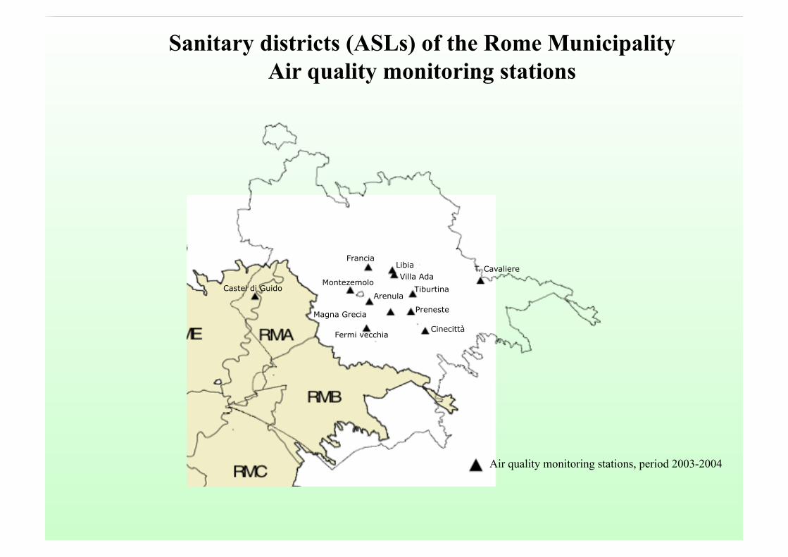
Sanitary districts (ASLs) of the Rome Municipality
Air quality monitoring stations, period 2003-2004
Francia
Arenula
Preneste
Villa AdaTiburtina
Cinecittà
Montezemolo
Magna Grecia
Fermi vecchia
Castel di Guido
T. CavaliereLibia
Air quality monitoring stations
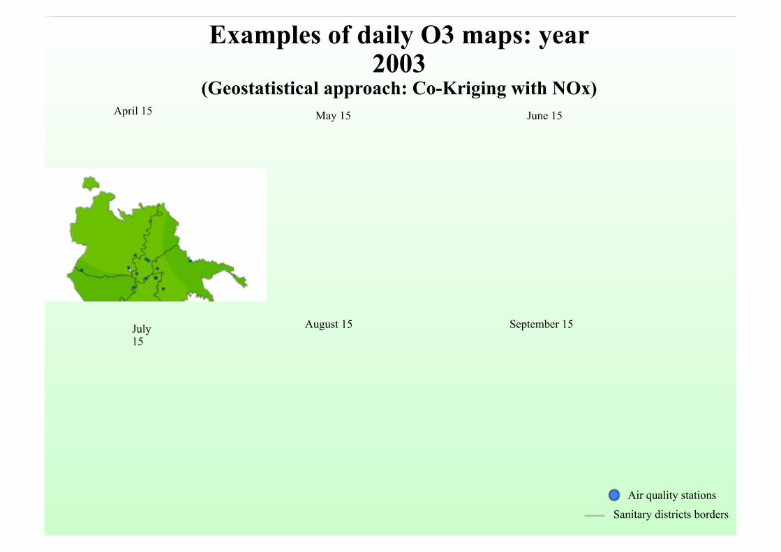
April 15 May 15 June 15
July15
August 15 September 15
Examples of daily O3 maps: year2003
(Geostatistical approach: Co-Kriging with NOx)
Air quality stations
Sanitary districts borders

Air quality stations
Sanitary districts borders
April 15 May 15 June 15
July15
August 15 September 15
Examples of daily O3 maps: year2004
(Geostatistical approach: Co-Kriging with NOx)
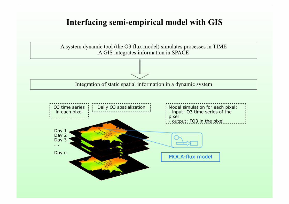
A system dynamic tool (the O3 flux model) simulates processes in TIMEA GIS integrates information in SPACE
Integration of static spatial information in a dynamic system
Daily O3 spatialization
Day 1Day 2Day 3…. Day n
MOCA-flux model
Model simulation for each pixel:- input: O3 time series of thepixel- output: FO3 in the pixel
O3 time seriesin each pixel
Interfacing semi-empirical model with GIS
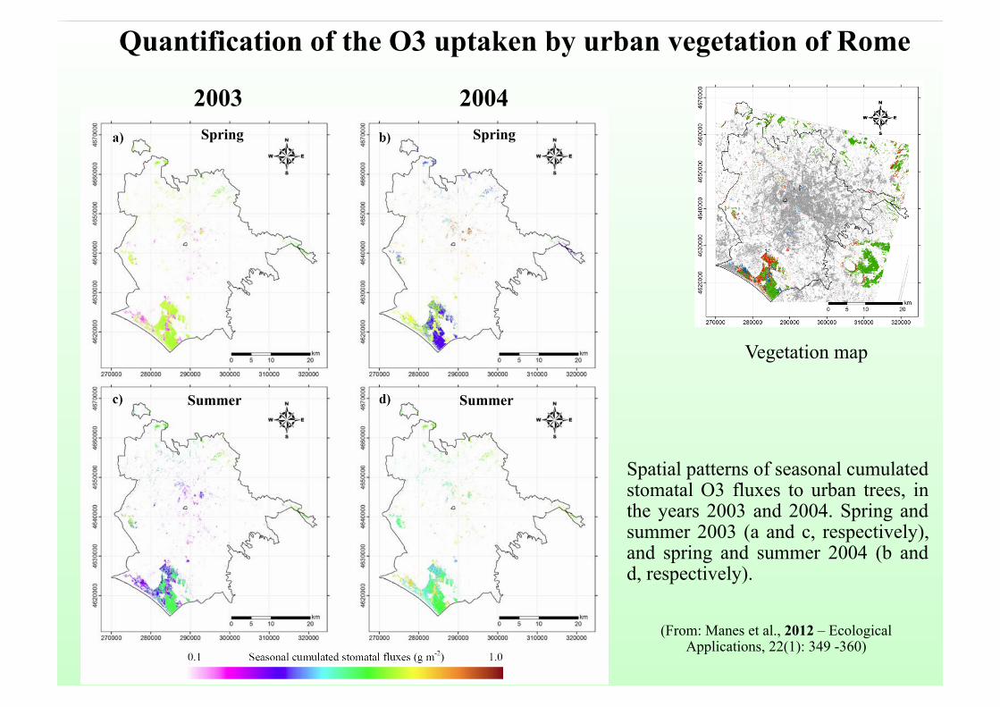
Quantification of the O3 uptaken by urban vegetation of Rome
Spatial patterns of seasonal cumulatedstomatal O3 fluxes to urban trees, inthe years 2003 and 2004. Spring andsummer 2003 (a and c, respectively),and spring and summer 2004 (b andd, respectively).
2003 2004Spring
Summer
Spring
Summer
Vegetation map
(From: Manes et al., 2012 – EcologicalApplications, 22(1): 349 -360)
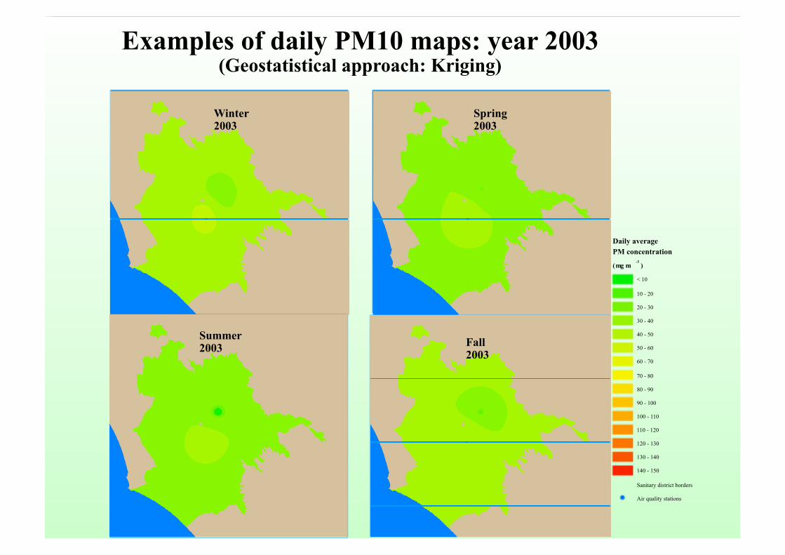
Winter2003
Spring2003
Summer2003
Fall2003
Air quality stations
Sanitary district borders
140 - 150
130 - 140
120 - 130
110 - 120
100 - 110
90 - 100
80 - 90
70 - 80
60 - 70
50 - 60
40 - 50
30 - 40
20 - 30
10 - 20
< 10
(mg m-3
)
Daily averagePM concentration
Examples of daily PM10 maps: year 2003(Geostatistical approach: Kriging)
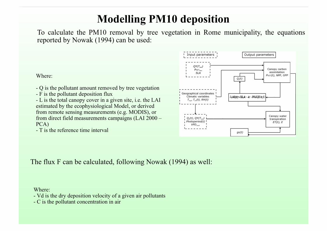
To calculate the PM10 removal by tree vegetation in Rome municipality, the equationsreported by Nowak (1994) can be used:
Where: - Q is the pollutant amount removed by tree vegetation- F is the pollutant deposition flux- L is the total canopy cover in a given site, i.e. the LAIestimated by the ecophysiological Model, or derivedfrom remote sensing measurements (e.g. MODIS), orfrom direct field measurements campaigns (LAI 2000 –PCA)- T is the reference time interval
The flux F can be calculated, following Nowak (1994) as well:
Where:- Vd is the dry deposition velocity of a given air pollutants- C is the pollutant concentration in air
Modelling PM10 deposition
LAI(t)=SLA · a · PNET(t-1)
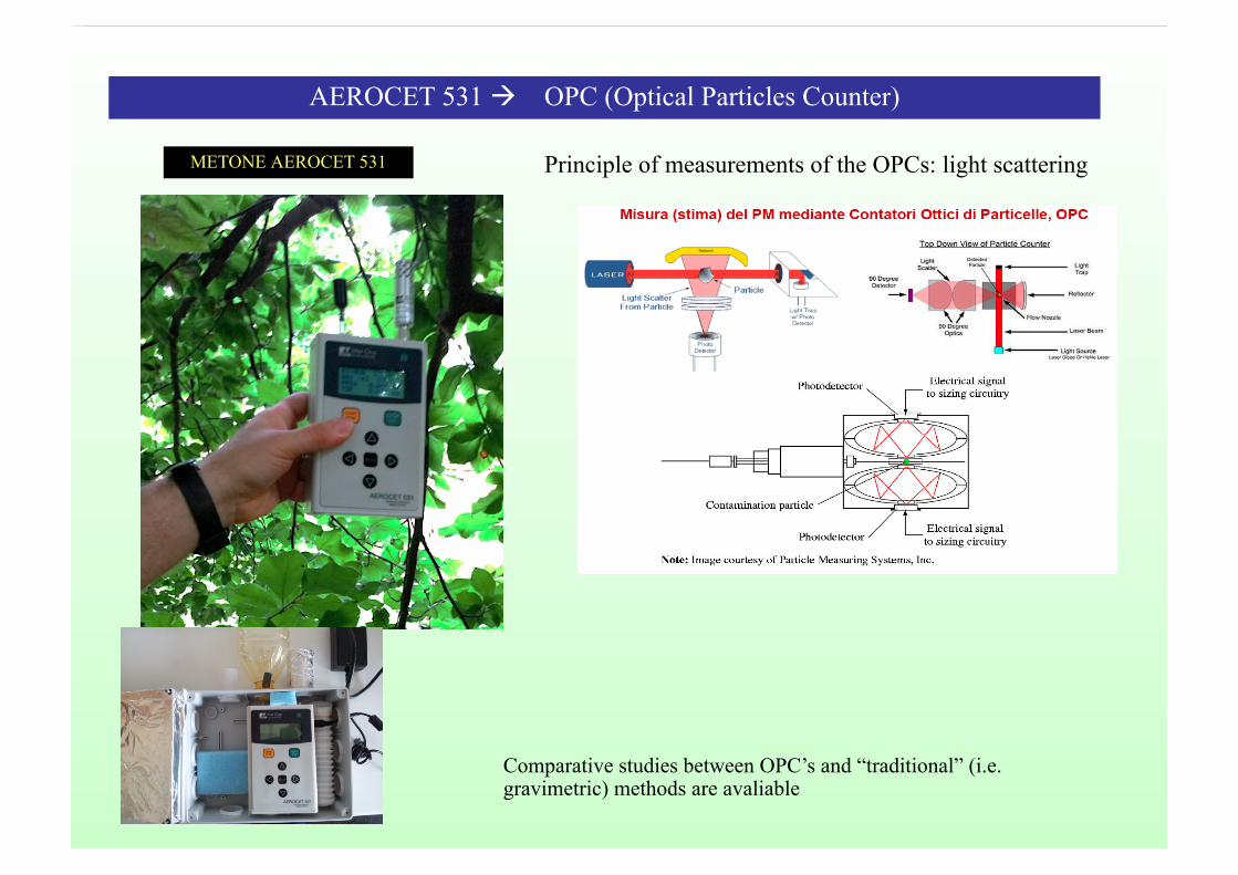
AEROCET 531 ! OPC (Optical Particles Counter)
METONE AEROCET 531
Comparative studies between OPC’s and “traditional” (i.e.gravimetric) methods are avaliable
Principle of measurements of the OPCs: light scattering
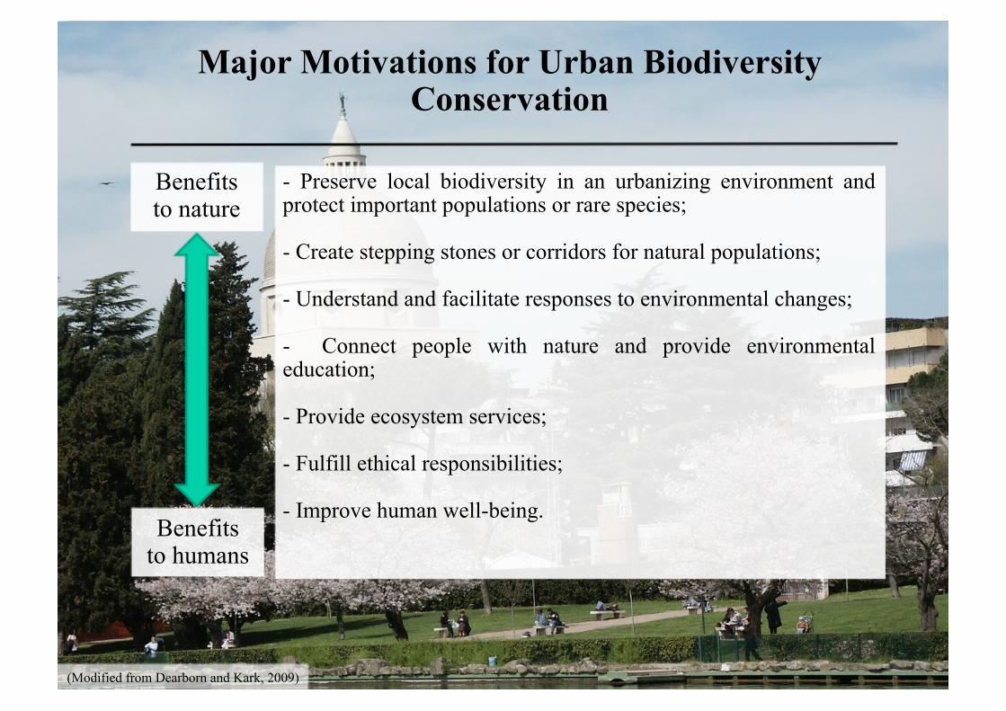
Benefitsto nature
Benefitsto humans
- Preserve local biodiversity in an urbanizing environment andprotect important populations or rare species; - Create stepping stones or corridors for natural populations; - Understand and facilitate responses to environmental changes; - Connect people with nature and provide environmentaleducation; - Provide ecosystem services; - Fulfill ethical responsibilities; - Improve human well-being.
Major Motivations for Urban BiodiversityConservation
(Modified from Dearborn and Kark, 2009)
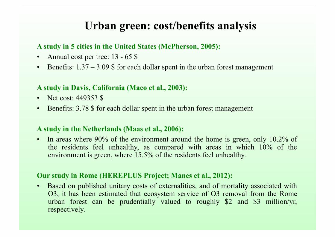
Urban green: cost/benefits analysis
A study in 5 cities in the United States (McPherson, 2005):• Annual cost per tree: 13 - 65 $• Benefits: 1.37 – 3.09 $ for each dollar spent in the urban forest management A study in Davis, California (Maco et al., 2003):• Net cost: 449353 $• Benefits: 3.78 $ for each dollar spent in the urban forest management A study in the Netherlands (Maas et al., 2006):• In areas where 90% of the environment around the home is green, only 10.2% of
the residents feel unhealthy, as compared with areas in which 10% of theenvironment is green, where 15.5% of the residents feel unhealthy.
Our study in Rome (HEREPLUS Project; Manes et al., 2012):• Based on published unitary costs of externalities, and of mortality associated with
O3, it has been estimated that ecosystem service of O3 removal from the Romeurban forest can be prudentially valued to roughly $2 and $3 million/yr,respectively.
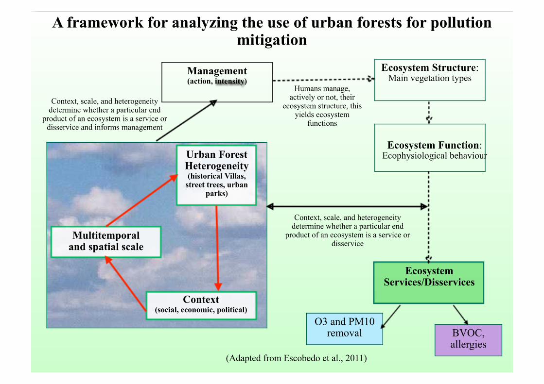
A framework for analyzing the use of urban forests for pollutionmitigation
Multitemporaland spatial scale
Urban ForestHeterogeneity(historical Villas,
street trees, urbanparks)
Context(social, economic, political)
Management(action, intensity)
Ecosystem Structure:Main vegetation types
Ecosystem Function:Ecophysiological behaviour
EcosystemServices/Disservices
Context, scale, and heterogeneitydetermine whether a particular end
product of an ecosystem is a service ordisservice and informs management
(Adapted from Escobedo et al., 2011)
Humans manage,actively or not, their
ecosystem structure, thisyields ecosystem
functions
Context, scale, and heterogeneitydetermine whether a particular end
product of an ecosystem is a service ordisservice
O3 and PM10removal BVOC,
allergies
Thank you for your attention!
Department of Environmental Biology,Sapienza University of Rome
Laboratory of Functional Ecology:
Fausto ManesElisabetta Salvatori
Lina FusaroValerio Silli
Gina GalanteGigliola PuppiCarlo Ricotta
Recommended