Embed Size (px)
Citation preview

Time-Varying Temporal Dependen e
in Autoregressive Models
F. Blasques S.J. Koopman A. Lu as
VU University Amsterdam, Tinbergen Institute, CREATES
International Asso iation for Applied E onometri s
2014 Annual Conferen e
Queen Mary, University of London, 26-28 June 2014
1 / 1 Blasques, Koopman and Lu as Time-Varying Temporal Dependen e

Motivation
For an observable time series y1, . . . , yT , we onsider the
standard autoregressive model of order one, the AR(1) model
yt = ϕyt−1 + ut, ut ∼ pu(ut;λ), t = 1, . . . , T,
where ϕ is the autoregressive oe� ient with stationary
ondition −1 < ϕ < 1 and where ut is the random error with
density fun tion pu(ut;λ) and parameter ve tor λ.
In many appli ations in e onomi s and �nan e, there is a quest
for ϕ to be time-varying, we have
yt = ϕtyt−1 + ut, ut ∼ pu(ut;λ), t = 1, . . . , T,
but what is an appropriate dynami spe i� ation for ϕt ?
2 / 1 Blasques, Koopman and Lu as Time-Varying Temporal Dependen e

Motivation
The time-varying dependen e in an AR(1) model,
yt = ϕtyt−1 + ut, ut ∼ pu(ut;λ), t = 1, . . . , T,
an be modelled expli itly via the link fun tion
ϕt = h(αt),
where αt is spe i�ed as another dynami pro ess, say
αt = Φαt−1 + ηt, ηt ∼ pη(ηt, λ), t = 1, . . . , T.
We regard this system of dynami equations as a onditional,
and possibly nonlinear, state spa e model.
Kalman �lter and maximum likelihood methods an be used.
3 / 1 Blasques, Koopman and Lu as Time-Varying Temporal Dependen e
Motivation
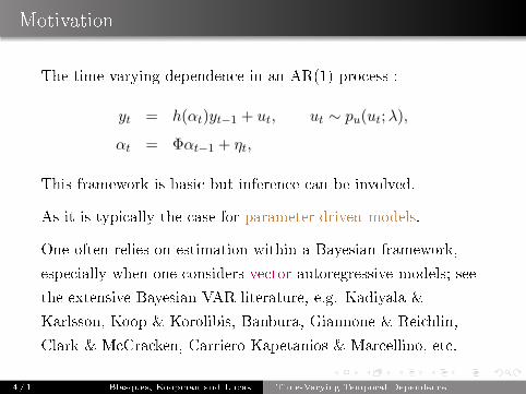
The time-varying dependen e in an AR(1) pro ess :
yt = h(αt)yt−1 + ut, ut ∼ pu(ut;λ),
αt = Φαt−1 + ηt,
This framework is basi but inferen e an be involved.
As it is typi ally the ase for parameter-driven models.
One often relies on estimation within a Bayesian framework,
espe ially when one onsiders ve tor autoregressive models; see
the extensive Bayesian VAR literature, e.g. Kadiyala &
Karlsson, Koop & Korolibis, Banbura, Giannone & Rei hlin,
Clark & M Cra ken, Carriero Kapetanios & Mar ellino, et .
4 / 1 Blasques, Koopman and Lu as Time-Varying Temporal Dependen e
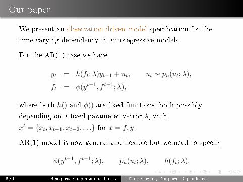
Our paper
We present an observation-driven model spe i� ation for the
time-varying dependen y in autoregressive models.
For the AR(1) ase we have
yt = h(ft;λ)yt−1 + ut, ut ∼ pu(ut;λ),
ft = φ(yt−1, f t−1;λ),
where both h() and φ() are �xed fun tions, both possibly
depending on a �xed parameter ve tor λ, with
xt = {xt, xt−1, xt−2, . . .} for x = f, y.
AR(1) model is now general and �exible but we need to spe ify
φ(yt−1, f t−1;λ), pu(ut;λ), h(ft;λ).
5 / 1 Blasques, Koopman and Lu as Time-Varying Temporal Dependen e

Time-varying temporal dependen e in AR(1) model
For the general and �exible AR(1) model
yt = h(ft;λ)yt−1 + ut, ut ∼ pu(ut;λ),
ft = φ(yt−1, f t−1;λ),
we take the linear updating equation
φ(yt−1, f t−1;λ) = ω + αs(yt−1, f t−1;λ) + βft−1,
where ω, α and β are �xed oe� ients and s(·, ·) is a
deterministi fun tion of past observations.
In parti ular, we take s(·, ·) as the s ore fun tion of the
onditional or predi tive log-density fun tion of yt,
log p(yt|ft, yt−1;λ) ≡ log pu(ut;λ),
as ut = yt − h(ft;λ)yt−1, with respe t to ft.6 / 1 Blasques, Koopman and Lu as Time-Varying Temporal Dependen e

Time-varying temporal dependen e in AR(1) model
Our time-varying temporal dependen e AR(1) model is given by
yt = h(ft;λ)yt−1 + ut, ut ∼ pu(ut;λ),
ft = ω + αs(yt−1, f t−1;λ) + βft−1,
with s ore fun tion
st ≡ s(yt, f t;λ) =∂ log p(yt|ft, y
t−1;λ)
∂ft.
In spirit of GAS model : Creal, Koopman & Lu as (2008,11,13).
Why the s ore ? It is optimal in Kullba k-Leibler sense, later !
But what about the hoi e for pu(ut;λ) and h(ft;λ) ?
7 / 1 Blasques, Koopman and Lu as Time-Varying Temporal Dependen e
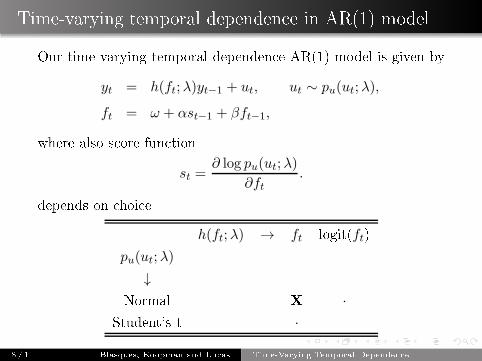
Time-varying temporal dependen e in AR(1) model
Our time-varying temporal dependen e AR(1) model is given by
yt = h(ft;λ)yt−1 + ut, ut ∼ pu(ut;λ),
ft = ω + αst−1 + βft−1,
where also s ore fun tion
st =∂ log pu(ut;λ)
∂ft.
depends on hoi e
h(ft;λ) → ft logit(ft)
pu(ut;λ)
↓
Normal X ·
Student's t ·
8 / 1 Blasques, Koopman and Lu as Time-Varying Temporal Dependen e
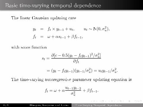
Basi time-varying temporal dependen e
The linear Gaussian updating ase
yt = ft × yt−1 + ut, ut ∼ N(0, σ2u),
ft = ω + αst−1 + βft−1,
with s ore fun tion
st =∂[c− 0.5(yt − ftyt−1)
2/σ2u]
∂ft
= (yt − ftyt−1)(yt−1/σ2u) = utyt−1/σ
2u.
The time-varying autoregressive parameter updating equation is
ft = ω + αut−1yt−2
σ2u
+ βft−1.
9 / 1 Blasques, Koopman and Lu as Time-Varying Temporal Dependen e

Basi time-varying temporal dependen e
We have the model
yt = ft × yt−1 + ut, ft = ω + αut−1yt−2
σ2u
+ βft−1.
Interesting interpretation :
update of ft rea ts to error ut−1 multiplied by yt−2 and
s aled by σ−2u .
role of yt−2 is to signal whether ft is below or above its
mean.
update distinguishes role of observed past data and of past
parameter value.
More interesting/intrinsi updating equations for other pu and h
10 / 1 Blasques, Koopman and Lu as Time-Varying Temporal Dependen e

Basi time-varying temporal dependen e
−2 0 2 4−0.2
0.4
1
−2 0 2 4
−2 0 2 4
N-GAS (β = 0.5) N-GAS (β = 1) t-GAS (β = 0.5) t-GAS (β = 1)
yt−2yt−2 yt−2
yt−1 yt−1 yt−1
ft−1
ft
Figure: Updating for ft: h(f) = f and pu(u) = N , t.
11 / 1 Blasques, Koopman and Lu as Time-Varying Temporal Dependen e

Redu ed form
Our basi time-varying temporal dependen e model
yt = ft × yt−1 + ut, ft = ω + αut−1yt−2
σ2u
+ βft−1,
is e�e tively a nonlinear ARMA model
yt =
{
ω + β
[
yt−1 − ut−1
yt−1
]}
yt−1 + ut + α
[
yt−1
σ2u
]
ut−1.
It is a nonlinear ARMA(2, 1) !
Some minor algebra is required to obtain this result.
Similar results an be obtained for the other ases.
12 / 1 Blasques, Koopman and Lu as Time-Varying Temporal Dependen e

Nonlinear ARMA models
We have shown that our basi time-varying temporal
dependen e model is a nonlinear ARMA model.
But what is new ? So many other nonlinear ARMA models !
Threshold AR � Tong (1991)
yt = ϕt × yt−1 + ut, ϕt = ϕ+ ϕ∗I(yt−2 < γ),
Smooth Transition � Chan & Tong (1986), Teräsvirta (1994)
yt = ϕt × yt−1 + ut, ϕt = γ1xt−2 + γ2(1− xt−2),
where xt = [1 + exp(−γ3 yt)]−1.
13 / 1 Blasques, Koopman and Lu as Time-Varying Temporal Dependen e

Comparison with TAR and STAR
14 / 1 Blasques, Koopman and Lu as Time-Varying Temporal Dependen e

Comparison with our basi model
15 / 1 Blasques, Koopman and Lu as Time-Varying Temporal Dependen e
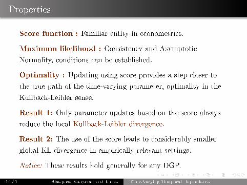
Properties
S ore fun tion : Familiar entity in e onometri s.
Maximum likelihood : Consisten y and Asymptoti
Normality, onditions an be established.
Optimality : Updating using s ore provides a step loser to
the true path of the time-varying parameter, optimality in the
Kullba k-Leibler sense.
Result 1: Only parameter updates based on the s ore always
redu e the lo al Kullba k-Leibler divergen e.
Result 2: The use of the s ore leads to onsiderably smaller
global KL divergen e in empiri ally relevant settings.
Noti e: These results hold generally for any DGP.
16 / 1 Blasques, Koopman and Lu as Time-Varying Temporal Dependen e

Optimal Observation-Driven Update
Key obje tive: Chara terize φ(·) that possess optimality
properties from information theoreti point of view.
Main Question: Is there an optimal form for the update
f̃t+1 = φ(
yt , f̃t ; θ)
, ∀ t ∈ N, f̃1 ∈ F ⊆ R,
Answer: This depends on the notion of optimality!
Result 1: Only parameter updates based on the s ore always
redu e the lo al Kullba k-Leibler divergen e p and p̃.
Result 2: The use of the s ore leads to onsiderably smaller
global KL divergen e in empiri ally relevant settings.
Note: Results hold for any DGP ( any p and {ft} )
17 / 1 Blasques, Koopman and Lu as Time-Varying Temporal Dependen e

De�nitions: Lo al GAS Updates
GAS-update:
f̃t+1 = φ(
yt , f̃t ; θ)
= ω + αs(yt, f̃t) + βf̃t, ∀ t ∈ N,
Newton-GAS update: ( ω = 0, α > 0, β = 1 )
f̃t+1 = αs(yt, f̃t) + f̃t, ∀ t ∈ N,
Lo al update: f̃t+1 in neighborhood of f̃t
Lo al optimality: Refers to lo al updates
18 / 1 Blasques, Koopman and Lu as Time-Varying Temporal Dependen e

De�nition I: Realized KL Divergen e
KL divergen e between p(·|ft) and p̃(
· |f̃t+1;θ)
is given by
DKL
(
p(·|ft) , p̃(
· |f̃t+1;θ)
)
=
∫
∞
−∞
p(yt|ft) lnp(yt|ft)
p̃(
yt|f̃t+1;θ) dyt.
19 / 1 Blasques, Koopman and Lu as Time-Varying Temporal Dependen e

De�nition I: Realized KL Divergen e
KL divergen e between p(·|ft) and p̃(
· |f̃t+1;θ)
is given by
DKL
(
p(·|ft) , p̃(
· |f̃t+1;θ)
)
=
∫
∞
−∞
p(yt|ft) lnp(yt|ft)
p̃(
yt|f̃t+1;θ) dyt.
The realized KL variation ∆t−1RKL
of a parameter update from f̃t
to f̃t+1 is de�ned as
∆t−1RKL
= DKL
(
p(·|ft) , p̃(
· |f̃t+1;θ)
)
−DKL
(
p(·|ft) , p̃(
· |f̃t;θ)
)
19 / 1 Blasques, Koopman and Lu as Time-Varying Temporal Dependen e

De�nition II: Conditionally Expe ted KL Divergen e
An optimal updating s heme, while subje t to randomness,
should have tenden y to move in orre t dire tion:
On average, the KL divergen e should redu e in expe tation.
20 / 1 Blasques, Koopman and Lu as Time-Varying Temporal Dependen e

De�nition II: Conditionally Expe ted KL Divergen e
An optimal updating s heme, while subje t to randomness,
should have tenden y to move in orre t dire tion:
On average, the KL divergen e should redu e in expe tation.
The onditionally expe ted KL (CKL) variation of a parameter
update from f̃t ∈ F̃ to f̃t+1 ∈ F̃ is given by
∆t−1CKL
=
∫
F
q(f̃t+1|f̃t, ft;θ)
[
∫
Y
p(y|ft) lnp̃(y|f̃t;θ)
p̃(y|f̃t+1;θ)dy
]
df̃t+1,
where q(f̃t+1|f̃t, ft;θ) denotes the density of f̃t+1 onditional on
both f̃t and ft. For a given pt, an update is CKL optimal if and
only if ∆t−1CKL
≤ 0.
20 / 1 Blasques, Koopman and Lu as Time-Varying Temporal Dependen e

Ba k to our basi model : ondition for RKL and CKL
Our basi time-varying temporal dependen e model
yt = ft × yt−1 + ut, ft = ω + αut−1yt−2
σ2u
+ βft−1,
we obtain RKL optimality under the ondition
α > σ2u
|ω + (β − 1)f̃t|
|(yt−1 − f̃t−1yt−2)yt−2|,
The new s ore information should have lo ally su� ient impa t
on the updating for ft.
A similar but di�erent ondition is derived for CKL optimality.
21 / 1 Blasques, Koopman and Lu as Time-Varying Temporal Dependen e

22 / 1 Blasques, Koopman and Lu as Time-Varying Temporal Dependen e

Empiri al illustration: Unemployment Insuran e Claims
We analyze the growth rate of US seasonally adjusted weekly
Unemployment Insuran e Claims (UIC) for roughly the last �ve
de ades.
Meyer (1995), Anderson & Meyer (1997, 2000), Hopenhayn &
Ni olini (1997) and Ashenfelter (2005) have studied the UIC
series.
The importan e of fore asting UIC has been highlighted by
Gavin & Kliesen (2002):
UIC is a leading indi ator for several labor market onditions:
how they an be used to fore asting GDP growth rates.
Here we onsider various models and do some omparisons
amongst them.
23 / 1 Blasques, Koopman and Lu as Time-Varying Temporal Dependen e

Empiri al illustration
Unemployment Insuran e Claims: Model Comparison
(N) AR-GAS TAR STAR AR(2) AR(5)
LL 6744 6736 6737 6439 6968
AIC -13478 -13462 -13464 -12870 -13921
RMSE 0.750 0.752 0.752 0.848 1.20
24 / 1 Blasques, Koopman and Lu as Time-Varying Temporal Dependen e

Empiri al results
2005 2006 2007 2008 2009 2010 2011 2012 2013
−0.05
0
0.05
Uemployment Insurance Claims
2005 2006 2007 2008 2009 2010 2011 2012 2013
0.4
0.5
0.6
Normal AR−GAS (Identity Link and Unit Scaling)
25 / 1 Blasques, Koopman and Lu as Time-Varying Temporal Dependen e

Con lusions
We have introdu ed time-varying temporal dependen e in the
AR(1) model
yt = ft × yt−1 + ut, ft = ω + αut−1yt−2
σ2u
+ βft−1,
an observation-driven approa h to time-varying
autoregressive oe� ient: GAS model is e�e tive !
redu ed form : nonlinear ARMA models
they an be ompared with TAR and STAR models
the �ltered estimate ft has optimality properties in the KL
sense when based on the s ore fun tion !
we provide some Monte Carlo eviden e
an empiri al illustration for UIC is presented
26 / 1 Blasques, Koopman and Lu as Time-Varying Temporal Dependen e

This project has received funding from the European Union’s
Seventh Framework Programme for research, technological
development and demonstration under grant agreement no° 320270
www.syrtoproject.eu
This document reflects only the author’s views.
The European Union is not liable for any use that may be made of the information contained therein.