Merge Sort

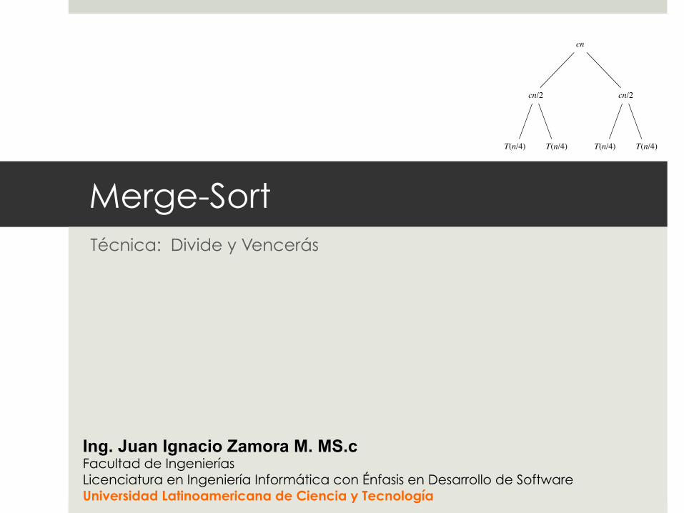
Merge-Sort Técnica: Divide y Vencerás

Ing. Juan Ignacio Zamora M. MS.c Facultad de Ingenierías Licenciatura en Ingeniería Informática con Énfasis en Desarrollo de Software Universidad Latinoamericana de Ciencia y Tecnología

2-14 Lecture Notes for Chapter 2: Getting Started

• Let c be a constant that describes the running time for the base case and also

is the time per array element for the divide and conquer steps. [Of course, we

cannot necessarily use the same constant for both. Itís not worth going into this

detail at this point.]

• We rewrite the recurrence as

T (n) =!c if n = 1 ,2T (n/2) + cn if n > 1 .

• Draw a recursion tree, which shows successive expansions of the recurrence.

• For the original problem, we have a cost of cn, plus the two subproblems, each

costing T (n/2):

cn

T(n/2) T(n/2)

• For each of the size-n/2 subproblems, we have a cost of cn/2, plus two sub-

problems, each costing T (n/4):

cn

cn/2

T(n/4) T(n/4)

cn/2

T(n/4) T(n/4)

• Continue expanding until the problem sizes get down to 1:

cn

cn

Ö

Total: cn lg n + cn

cn

lg n

cn

n

c c c c c c c

Ö

cn

cn/2

cn/4 cn/4

cn/2

cn/4 cn/4

Técnica: Divide y Vencerás

¤  Técnica para resolución de problemas computaciones por medio de la descomposición del problema en instancias equivalentes pero de menor tamaño.

¤  La técnica se basa en 3 pasos conceptuales ¤  Dividir el problema en sub problemas

¤  Conquistar cada problema de forma recursiva

¤  Combinar todas las soluciones para solucionar el problema original

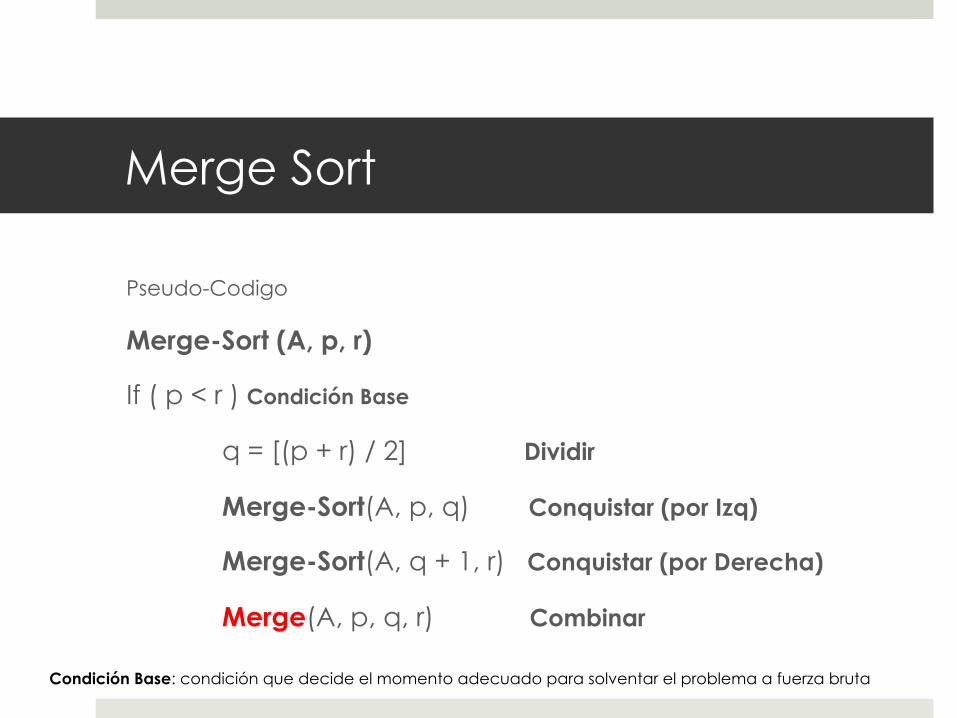
Merge Sort

Pseudo-Codigo

Merge-Sort (A, p, r)

If ( p < r ) Condición Base

q = [(p + r) / 2] Dividir

Merge-Sort(A, p, q) Conquistar (por Izq)

Merge-Sort(A, q + 1, r) Conquistar (por Derecha)

Merge(A, p, q, r) Combinar

Condición Base: condición que decide el momento adecuado para solventar el problema a fuerza bruta

Demostración Conceptual

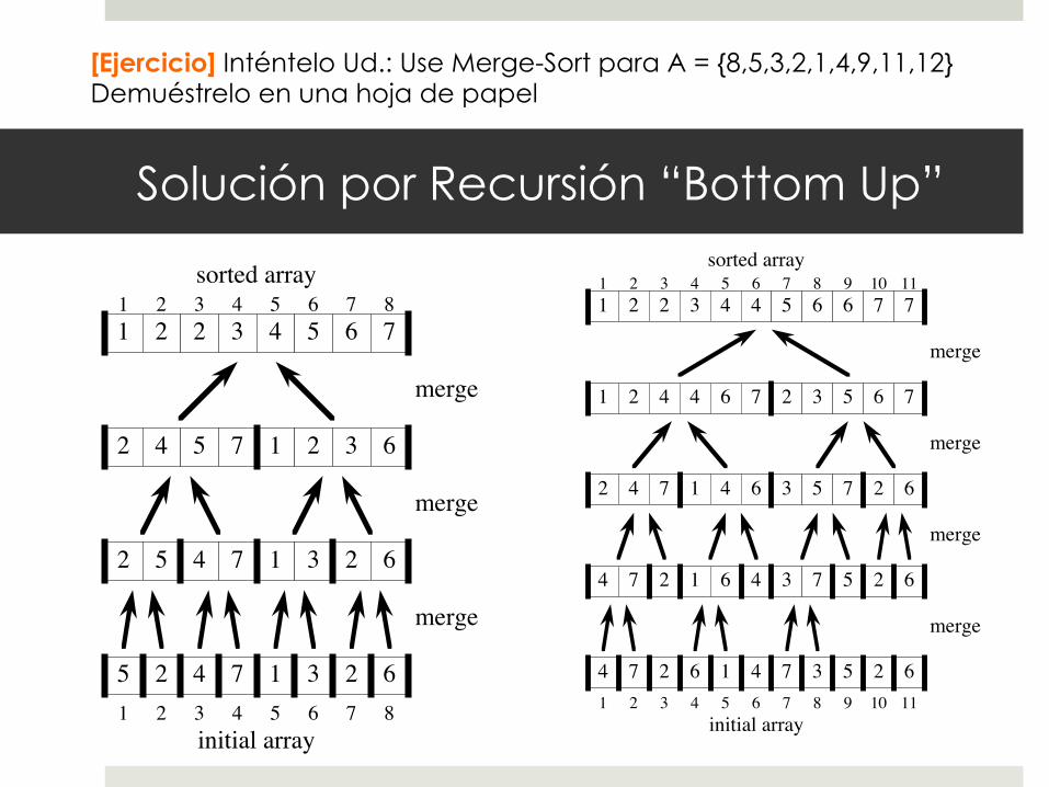
Solución por Recursión “Bottom Up”

Lecture Notes for Chapter 2: Getting Started 2-9

Merge sort

A sorting algorithm based on divide and conquer. Its worst-case running time hasa lower order of growth than insertion sort.

Because we are dealing with subproblems, we state each subproblem as sortinga subarray A[p . . r]. Initially, p = 1 and r = n, but these values change as werecurse through subproblems.

To sort A[p . . r]:

Divide by splitting into two subarrays A[p . . q] and A[q + 1 . . r], where q is thehalfway point of A[p . . r].

Conquer by recursively sorting the two subarrays A[p . . q] and A[q + 1 . . r].

Combine by merging the two sorted subarrays A[p . . q] and A[q + 1 . . r] to pro-duce a single sorted subarray A[p . . r]. To accomplish this step, weíll define aprocedure MERGE(A, p, q, r).

The recursion bottoms out when the subarray has just 1 element, so that itís triviallysorted.

MERGE-SORT(A, p, r)if p < r ! Check for base casethen q ! "(p + r)/2# ! Divide

MERGE-SORT(A, p, q) ! ConquerMERGE-SORT(A, q + 1, r) ! ConquerMERGE(A, p, q, r) ! Combine

Initial call: MERGE-SORT(A, 1, n)[It is astounding how often students forget how easy it is to compute the halfwaypoint of p and r as their average (p + r)/2. We of course have to take the floorto ensure that we get an integer index q. But it is common to see students performcalculations like p+ (r $ p)/2, or even more elaborate expressions, forgetting theeasy way to compute an average.]

Example: Bottom-up view for n = 8: [Heavy lines demarcate subarrays used insubproblems.]

1 2 3 4 5 6 7 8

5 2 4 7 1 3 2 6

2 5 4 7 1 3 2 6

initial array

merge

2 4 5 7 1 2 3 6

merge

1 2 3 4 5 6 7

merge

sorted array

21 2 3 4 5 6 7 8


[Examples when n is a power of 2 are most straightforward, but students mightalso want an example when n is not a power of 2.]Bottom-up view for n = 11:

1 2 3 4 5 6 7 8

4 7 2 6 1 4 7 3

initial array

merge

merge

merge

sorted array

5 2 69 10 11

4 7 2 1 6 4 3 7 5 2 6

2 4 7 1 4 6 3 5 7 2 6

1 2 4 4 6 7 2 3 5 6 7

1 2 2 3 4 4 5 6 6 7 71 2 3 4 5 6 7 8 9 10 11

merge

[Here, at the next-to-last level of recursion, some of the subproblems have only 1element. The recursion bottoms out on these single-element subproblems.]

Merging

What remains is the MERGE procedure.

Input: Array A and indices p, q, r such that• p ! q < r .• Subarray A[p . . q] is sorted and subarray A[q + 1 . . r] is sorted. By the

restrictions on p, q, r , neither subarray is empty.

Output: The two subarrays are merged into a single sorted subarray in A[p . . r].

We implement it so that it takes !(n) time, where n = r " p+ 1 = the number ofelements being merged.What is n? Until now, n has stood for the size of the original problem. But nowweíre using it as the size of a subproblem. We will use this technique when weanalyze recursive algorithms. Although we may denote the original problem sizeby n, in general n will be the size of a given subproblem.

Idea behind linear-time merging: Think of two piles of cards.• Each pile is sorted and placed face-up on a table with the smallest cards on top.• We will merge these into a single sorted pile, face-down on the table.• A basic step:

• Choose the smaller of the two top cards.

[Ejercicio] Inténtelo Ud.: Use Merge-Sort para A = {8,5,3,2,1,4,9,11,12} Demuéstrelo en una hoja de papel

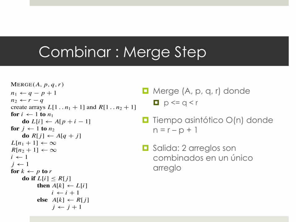
Combinar : Merge Step

¤  Merge (A, p, q, r) donde ¤  p <= q < r

¤  Tiempo asintótico O(n) donde n = r – p + 1

¤  Salida: 2 arreglos son combinados en un único arreglo


• Remove it from its pile, thereby exposing a new top card.• Place the chosen card face-down onto the output pile.

• Repeatedly perform basic steps until one input pile is empty.• Once one input pile empties, just take the remaining input pile and place itface-down onto the output pile.

• Each basic step should take constant time, since we check just the two top cards.• There are ! n basic steps, since each basic step removes one card from theinput piles, and we started with n cards in the input piles.

• Therefore, this procedure should take !(n) time.We donít actually need to check whether a pile is empty before each basic step.• Put on the bottom of each input pile a special sentinel card.• It contains a special value that we use to simplify the code.• We use", since thatís guaranteed to ìloseî to any other value.• The only way that" cannot lose is when both piles have " exposed as theirtop cards.

• But when that happens, all the nonsentinel cards have already been placed intothe output pile.

• We know in advance that there are exactly r # p + 1 nonsentinel cards$ stoponce we have performed r # p + 1 basic steps. Never a need to check forsentinels, since theyíll always lose.

• Rather than even counting basic steps, just fill up the output array from index pup through and including index r .

Pseudocode:

MERGE(A, p, q, r)n1% q # p + 1n2% r # qcreate arrays L[1 . . n1 + 1] and R[1 . . n2 + 1]for i % 1 to n1

do L[i]% A[p + i # 1]for j % 1 to n2

do R[ j ]% A[q + j ]L[n1 + 1]%"R[n2 + 1]%"i % 1j % 1for k % p to r

do if L[i] ! R[ j ]then A[k]% L[i]

i % i + 1else A[k]% R[ j ]

j % j + 1

[The book uses a loop invariant to establish that MERGE works correctly. In alecture situation, it is probably better to use an example to show that the procedureworks correctly.]

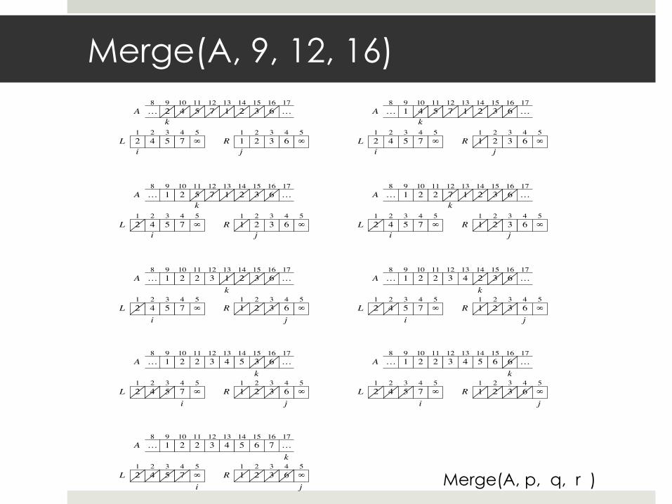
Merge(A, 9, 12, 16) 2-12 Lecture Notes for Chapter 2: Getting Started

Example: A call of MERGE(9, 12, 16)

A

L R1 2 3 4 1 2 3 4

i j

k

2 4 5 7 1 2 3 6

A

L R1 2 3 4 1 2 3 4

i j

k

2 4 5 7

1

2 3 61

2 4 5 7 1 2 3 6 4 5 7 1 2 3 6

A

L R

9 10 11 12 13 14 15 16

1 2 3 4 1 2 3 4

i j

k

2 4 5 7

1

2 3 61

5 7 1 2 3 62 A

L R1 2 3 4 1 2 3 4

i j

k

2 4 5 7

1

2 3 61

7 1 2 3 62 2

5

∞5

∞5

∞5

∞

5

∞5

∞5

∞5

∞

9 10 11 12 13 14 15 16

9 10 11 12 13 14 15 16

9 10 11 12 13 14 15 168Ö

17Ö

8Ö

17Ö

8Ö

17Ö

8Ö

17Ö

A

L R1 2 3 4 1 2 3 4

i j

k

2 4 5 7

1

2 3 61

1 2 3 62 2 3 A

L R1 2 3 4 1 2 3 4

i j

k

2 4 5 7

1

2 3 61

2 3 62 2 3 4

A

L R1 2 3 4 1 2 3 4

i j

k

2 4 5 7

1

2 3 61

3 62 2 3 4 5 A

L R1 2 3 4 1 2 3 4

i j

k

2 4 5 7

1

2 3 61

62 2 3 4 5

5

∞5

∞5

∞5

∞

5

∞5

∞5

∞5

∞

6

A

L R1 2 3 4 1 2 3 4

i j

k

2 4 5 7

1

2 3 61

72 2 3 4 5

5

∞5

∞

6

9 10 11 12 13 14 15 16

9 10 11 12 13 14 15 16

9 10 11 12 13 14 15 16

9 10 11 12 13 14 15 16

9 10 11 12 13 14 15 16

8Ö

17Ö

8Ö

17Ö

8Ö

17Ö

8Ö

17Ö

8Ö

17Ö

[Read this figure row by row. The first part shows the arrays at the start of theìfor k ! p to rî loop, where A[p . . q] is copied into L[1 . . n1] and A[q+1 . . r] iscopied into R[1 . . n2]. Succeeding parts show the situation at the start of successiveiterations. Entries in A with slashes have had their values copied to either L or Rand have not had a value copied back in yet. Entries in L and R with slashes havebeen copied back into A. The last part shows that the subarrays are merged backinto A[p . . r], which is now sorted, and that only the sentinels (") are exposed inthe arrays L and R.]

Running time: The first two for loops take !(n1+ n2) = !(n) time. The last forloop makes n iterations, each taking constant time, for !(n) time.Total time: !(n).

Merge(A, p, q, r )

Rendimiento Merge-Sort

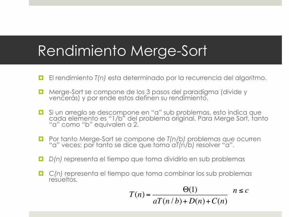
¤  El rendimiento T(n) esta determinado por la recurrencia del algoritmo.

¤  Merge-Sort se compone de los 3 pasos del paradigma (divide y vencerás) y por ende estos definen su rendimiento.

¤  Si un arreglo se descompone en “a” sub problemas, esto indica que cada elemento es “1/b” del problema original. Para Merge Sort, tanto “a” como “b” equivalen a 2.

¤  Por tanto Merge-Sort se compone de T(n/b) problemas que ocurren “a” veces; por tanto se dice que toma aT(n/b) resolver “a”.

¤  D(n) representa el tiempo que toma dividirlo en sub problemas

¤  C(n) representa el tiempo que toma combinar los sub problemas resueltos.

T (n) = Θ(1)aT (n / b)+D(n)+C(n)

n ≤ c

Rendimiento Merge-Sort

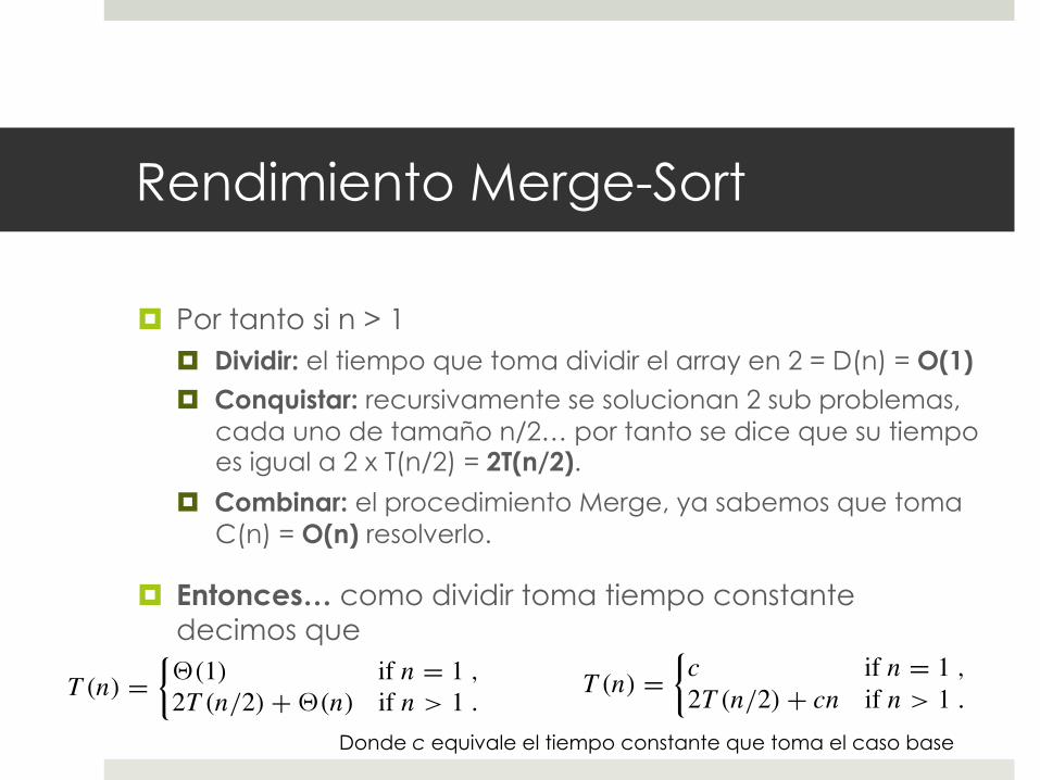
¤  Por tanto si n > 1 ¤  Dividir: el tiempo que toma dividir el array en 2 = D(n) = O(1) ¤  Conquistar: recursivamente se solucionan 2 sub problemas,

cada uno de tamaño n/2… por tanto se dice que su tiempo es igual a 2 x T(n/2) = 2T(n/2).

¤  Combinar: el procedimiento Merge, ya sabemos que toma C(n) = O(n) resolverlo.

¤  Entonces… como dividir toma tiempo constante decimos que


Analyzing divide-and-conquer algorithms

Use a recurrence equation (more commonly, a recurrence) to describe the runningtime of a divide-and-conquer algorithm.

Let T (n) = running time on a problem of size n.• If the problem size is small enough (say, n ! c for some constant c), we have abase case. The brute-force solution takes constant time: !(1).

• Otherwise, suppose that we divide into a subproblems, each 1/b the size of theoriginal. (In merge sort, a = b = 2.)

• Let the time to divide a size-n problem be D(n).• There are a subproblems to solve, each of size n/b" each subproblem takes

T (n/b) time to solve" we spend aT (n/b) time solving subproblems.• Let the time to combine solutions be C(n).• We get the recurrence

T (n) =!!(1) if n ! c ,aT (n/b) + D(n) + C(n) otherwise .

Analyzing merge sort

For simplicity, assume that n is a power of 2" each divide step yields two sub-problems, both of size exactly n/2.The base case occurs when n = 1.

When n # 2, time for merge sort steps:Divide: Just compute q as the average of p and r " D(n) = !(1).

Conquer: Recursively solve 2 subproblems, each of size n/2" 2T (n/2).Combine: MERGE on an n-element subarray takes !(n) time" C(n) = !(n).

Since D(n) = !(1) and C(n) = !(n), summed together they give a function thatis linear in n: !(n)" recurrence for merge sort running time is

T (n) =!!(1) if n = 1 ,2T (n/2) + !(n) if n > 1 .

Solving the merge-sort recurrence: By the master theorem in Chapter 4, we canshow that this recurrence has the solution T (n) = !(n lg n). [Reminder: lg nstands for log2 n.]Compared to insertion sort (!(n2) worst-case time), merge sort is faster. Tradinga factor of n for a factor of lg n is a good deal.On small inputs, insertion sort may be faster. But for large enough inputs, mergesort will always be faster, because its running time grows more slowly than inser-tion sortís.

We can understand how to solve the merge-sort recurrence without the master the-orem.


• Let c be a constant that describes the running time for the base case and also

is the time per array element for the divide and conquer steps. [Of course, we

cannot necessarily use the same constant for both. Itís not worth going into this

detail at this point.]

• We rewrite the recurrence as

T (n) =!c if n = 1 ,2T (n/2) + cn if n > 1 .

• Draw a recursion tree, which shows successive expansions of the recurrence.

• For the original problem, we have a cost of cn, plus the two subproblems, each

costing T (n/2):

cn

T(n/2) T(n/2)

• For each of the size-n/2 subproblems, we have a cost of cn/2, plus two sub-

problems, each costing T (n/4):

cn

cn/2

T(n/4) T(n/4)

cn/2

T(n/4) T(n/4)

• Continue expanding until the problem sizes get down to 1:

cn

cn

Ö

Total: cn lg n + cn

cn

lg n

cn

n

c c c c c c c

Ö

cn

cn/2

cn/4 cn/4

cn/2

cn/4 cn/4

Donde c equivale el tiempo constante que toma el caso base

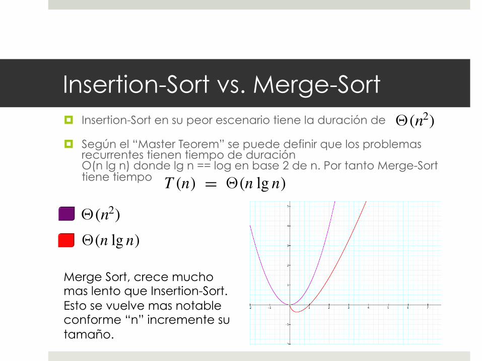
Insertion-Sort vs. Merge-Sort ¤  Insertion-Sort en su peor escenario tiene la duración de

¤  Según el “Master Teorem” se puede definir que los problemas recurrentes tienen tiempo de duración O(n lg n) donde lg n == log en base 2 de n. Por tanto Merge-Sort tiene tiempo














T (n) =!!(1) if n = 1 ,2T (n/2) + !(n) if n > 1 .
















T (n) =!!(1) if n = 1 ,2T (n/2) + !(n) if n > 1 .



Merge Sort, crece mucho mas lento que Insertion-Sort. Esto se vuelve mas notable conforme “n” incremente su tamaño.














T (n) =!!(1) if n = 1 ,2T (n/2) + !(n) if n > 1 .
















T (n) =!!(1) if n = 1 ,2T (n/2) + !(n) if n > 1 .



Merge-Sort es el campeón de la semana. Próximos contendientes … Heap-Sort, Quick-Sort…

Tarea Problemas de la Semana 1.  Programar el algoritmo de

“BubleSort” en su lenguaje de preferencia. Calcular el tiempo asintótico y compararlo contra MergeSort. Cual prefiere? Explique su respuesta!

Continua…

Tarea

Problemas de la Semana

2. Demuestre con argumentos lógicos si una búsqueda binaria puede ser escrita bajo el paradigma de divide y venceras…? (pista revisar capitulo 12)

3. Calcular el tiempo asintótico de los problemas [Carry Operations, Jolly Jumper y el Palíndromo de 2 números de 3 dígitos. 4. Leer Capítulos 4 (divide and conquer), 6 (heapsort) y 7 (quicksort).

Temas de Exposición Grupal

¤  Algoritmo Torres de Hanói

¤  “Divide and Conquer” orientado a Parallel Programming << ejemplo: Merge Sort Multihilo >>

¤  Algoritmo de Disjktra

¤  Transformación de Fourier*

¤  Radix-Sort

¤  Bucket-Sort

¤  Geometría Computacional*

¤  String Matching con Autómatas Finitos*

¤  Multiplicación Binaria usando “Divide and Conquer”

¤  Algoritmo Bellman-Ford*

Education

Merge Sort