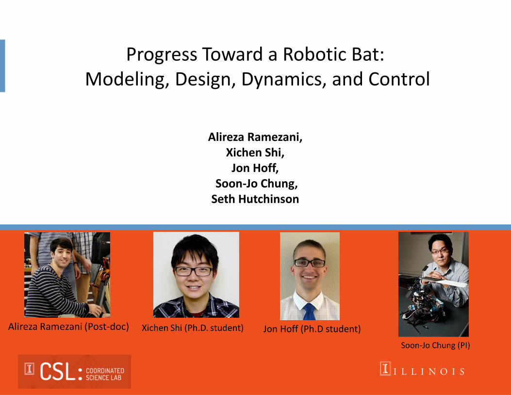
Progress Toward a Robotic Bat: Modeling, Design, Dynamics, and Control

Alireza Ramezani, Xichen Shi, Jon Hoff,

Soon-Jo Chung, Seth Hutchinson

Jon Hoff (Ph.D student)

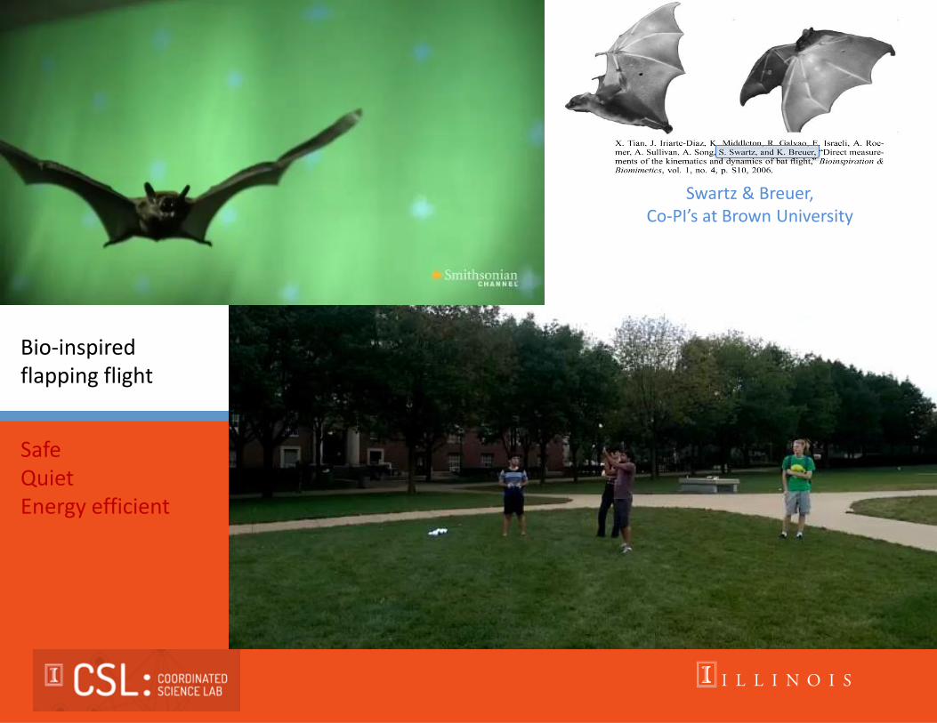
Swartz & Breuer, Co-PI’s at Brown University

Bio-inspired flapping flight

Safe Quiet Energy efficient

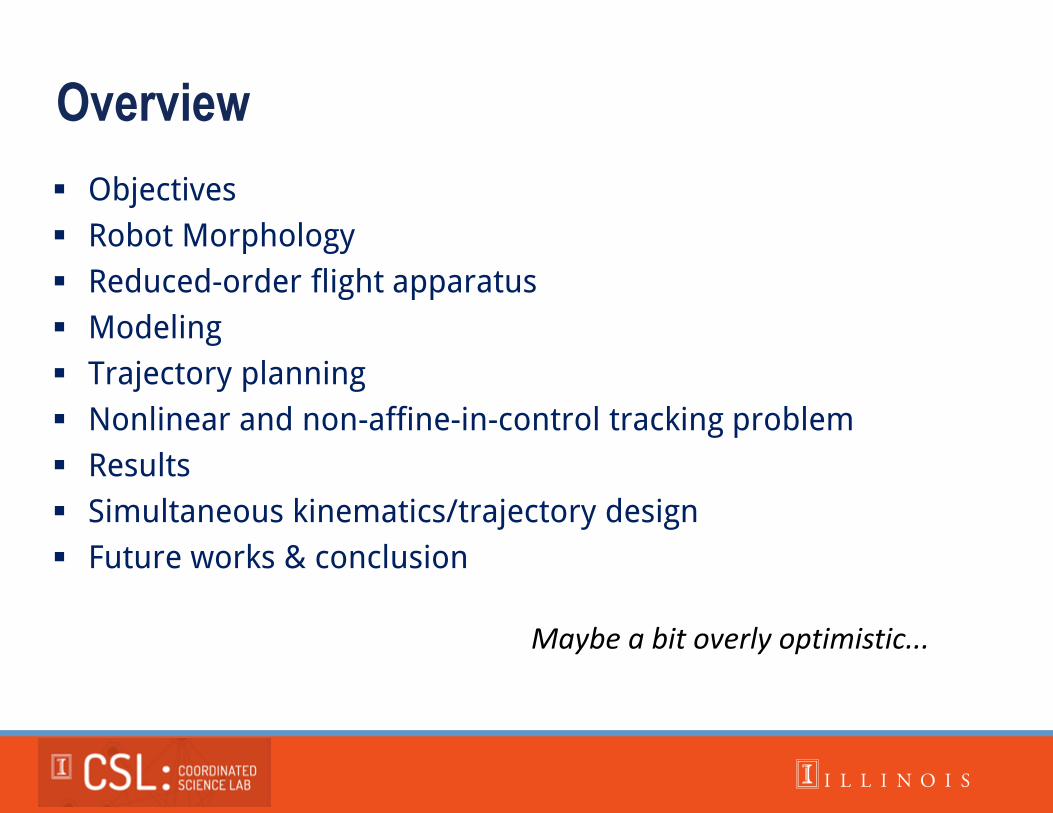
Overview

Objectives

Robot Morphology

Reduced-order flight apparatus

Modeling

Trajectory planning

Nonlinear and non-affine-in-control tracking problem

Results

Simultaneous kinematics/trajectory design

Future works & conclusion

Maybe a bit overly optimistic...

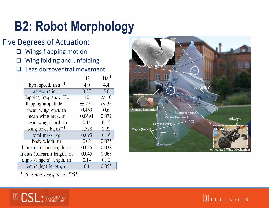
B2: Robot Morphology Five Degrees of Actuation:

Wings flapping motion

Wing folding and unfolding

Legs dorsoventral movement

B2: Robot Morphology Articulated Flight Mechanism

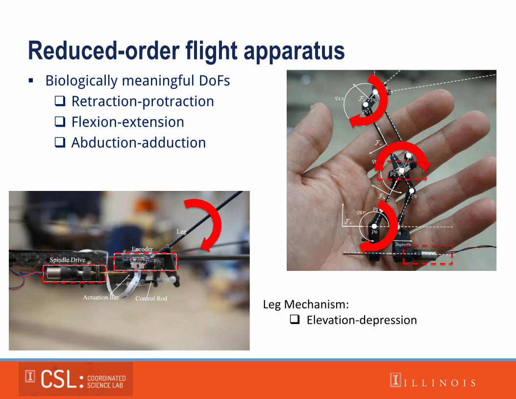
Reduced-order flight apparatus Biologically meaningful DoFs

Retraction-protraction

Flexion-extension

Abduction-adduction

Leg Mechanism: Elevation-depression

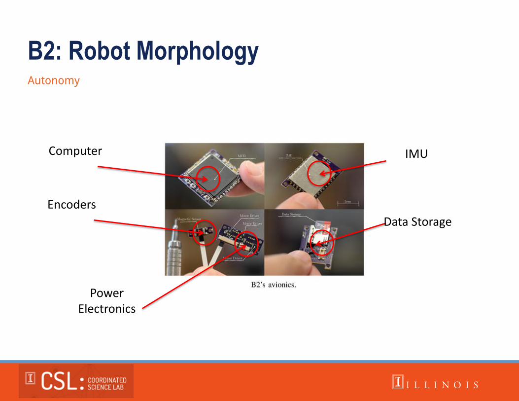
B2: Robot Morphology Autonomy

Computer

Encoders

Power Electronics

IMU

Data Storage

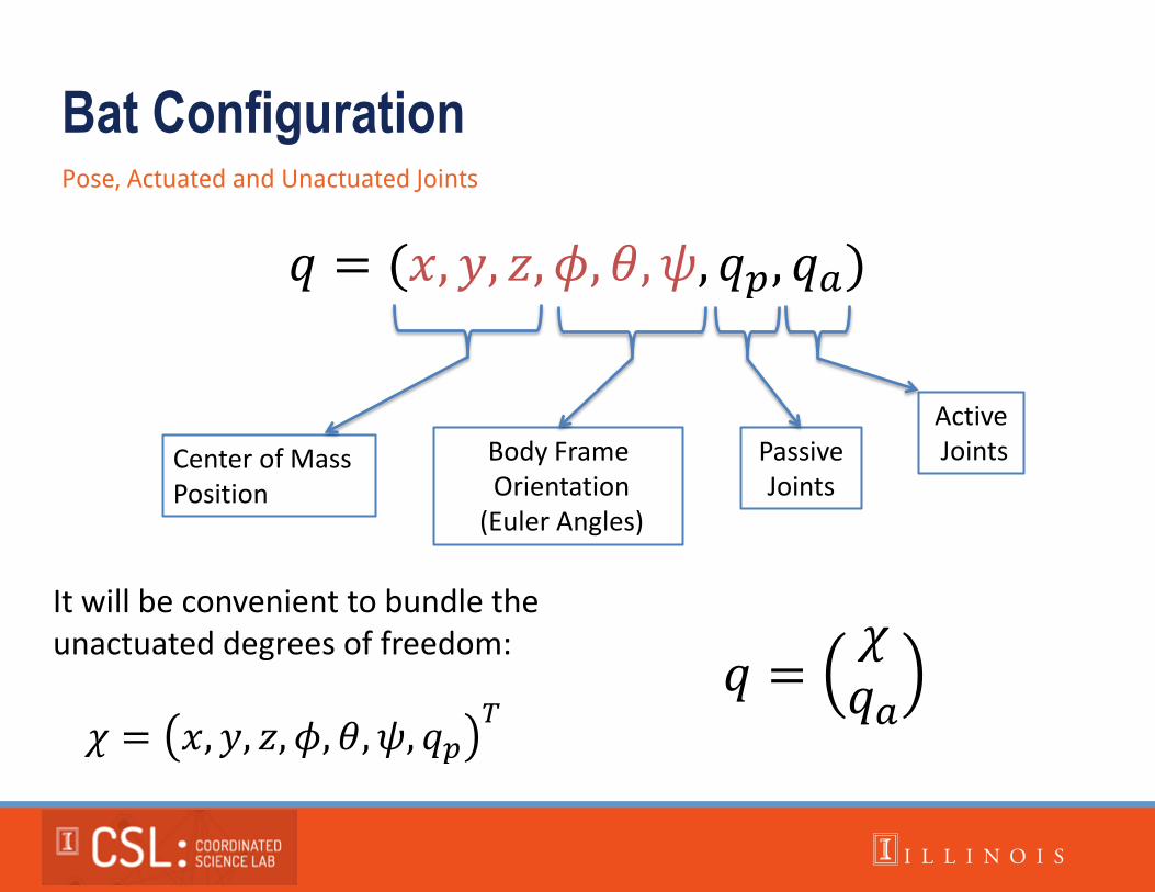
Bat Configuration Pose, Actuated and Unactuated Joints

𝑞 = (𝑥, 𝑦, 𝑧, 𝜙, 𝜃, 𝜓, 𝑞𝑝, 𝑞𝑎)

Center of Mass Position

Body Frame Orientation

(Euler Angles)

Passive Joints

Active Joints

𝜒 = 𝑥, 𝑦, 𝑧, 𝜙, 𝜃, 𝜓, 𝑞𝑝𝑇

It will be convenient to bundle the unactuated degrees of freedom:

𝑞 =𝜒𝑞𝑎

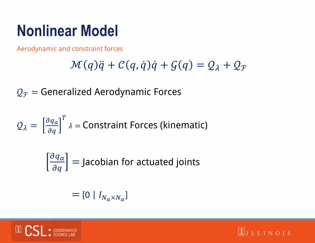
Nonlinear Model Aerodynamic and constraint forces

ℳ 𝑞 𝑞 + 𝒞 𝑞, 𝑞 𝑞 + 𝒢 𝑞 = 𝒬𝜆 + 𝒬ℱ

𝒬ℱ = Generalized Aerodynamic Forces

𝒬𝜆 = 𝜕𝑞𝑎

𝜕𝑞

𝑇𝜆 = Constraint Forces (kinematic)

𝜕𝑞𝑎

𝜕𝑞= Jacobian for actuated joints

= [0 | 𝐼𝑁𝑎×𝑁𝑎]

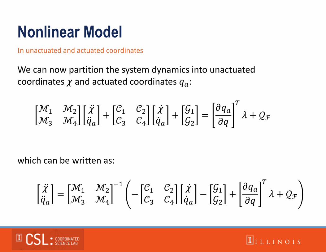
Nonlinear Model In unactuated and actuated coordinates

We can now partition the system dynamics into unactuated coordinates 𝜒 and actuated coordinates 𝑞𝑎:

ℳ1 ℳ2

ℳ3 ℳ4

𝜒 𝑞 𝑎

+𝒞1 𝒞2𝒞3 𝒞4

𝜒 𝑞 𝑎

+𝒢1𝒢2

=𝜕𝑞𝑎𝜕𝑞

𝑇

𝜆 + 𝒬ℱ

which can be written as:

𝜒 𝑞 𝑎

=ℳ1 ℳ2

ℳ3 ℳ4

−1

−𝒞1 𝒞2𝒞3 𝒞4

𝜒 𝑞 𝑎

−𝒢1𝒢2

+𝜕𝑞𝑎𝜕𝑞

𝑇

𝜆 + 𝒬ℱ

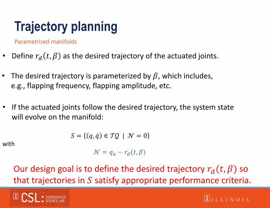
Trajectory planning Parametrized manifolds

• Define 𝑟𝑑 𝑡, 𝛽 as the desired trajectory of the actuated joints.

• The desired trajectory is parameterized by 𝛽, which includes, e.g., flapping frequency, flapping amplitude, etc.

• If the actuated joints follow the desired trajectory, the system state will evolve on the manifold:

𝑆 = 𝑞, 𝑞 ∈ 𝒯𝒬 | 𝒩 = 0 with

𝒩 = 𝑞𝑎 − 𝑟𝑑(𝑡, 𝛽)

Our design goal is to define the desired trajectory 𝑟𝑑(𝑡, 𝛽) so that trajectories in 𝑆 satisfy appropriate performance criteria.

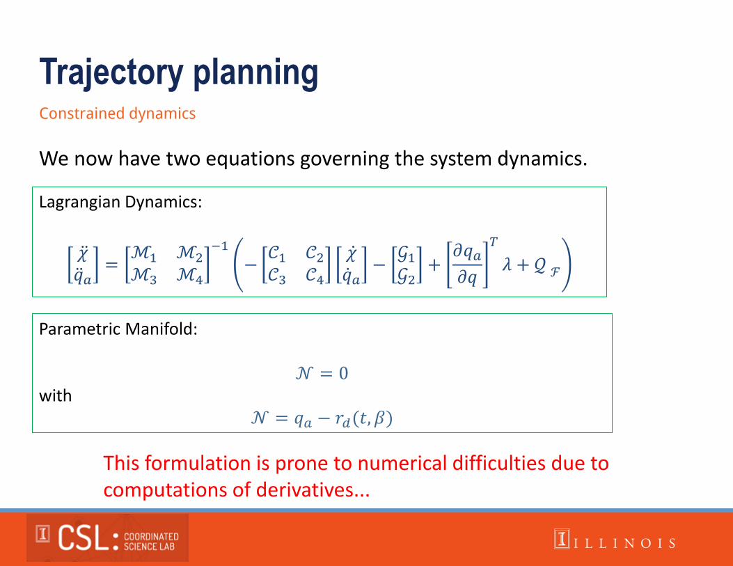
Trajectory planning Constrained dynamics

Parametric Manifold:

𝒩 = 0 with

𝒩 = 𝑞𝑎 − 𝑟𝑑(𝑡, 𝛽)

We now have two equations governing the system dynamics.

Lagrangian Dynamics:

𝜒 𝑞 𝑎

=ℳ1 ℳ2

ℳ3 ℳ4

−1

−𝒞1 𝒞2𝒞3 𝒞4

𝜒 𝑞 𝑎

−𝒢1𝒢2

+𝜕𝑞𝑎𝜕𝑞

𝑇

𝜆 + 𝒬 ℱ

This formulation is prone to numerical difficulties due to computations of derivatives...

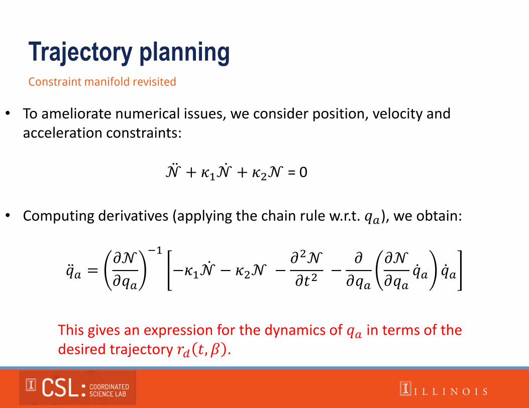
Trajectory planning Constraint manifold revisited

• To ameliorate numerical issues, we consider position, velocity and acceleration constraints:

𝒩 + 𝜅1𝒩 + 𝜅2𝒩 = 0

• Computing derivatives (applying the chain rule w.r.t. 𝑞𝑎), we obtain:

𝑞 𝑎 =𝜕𝒩

𝜕𝑞𝑎

−1

−𝜅1𝒩 − 𝜅2𝒩 −𝜕2𝒩

𝜕𝑡2 −

𝜕

𝜕𝑞𝑎

𝜕𝒩

𝜕𝑞𝑎𝑞 𝑎 𝑞 𝑎

This gives an expression for the dynamics of 𝑞𝑎 in terms of the desired trajectory 𝑟𝑑 𝑡, 𝛽 .

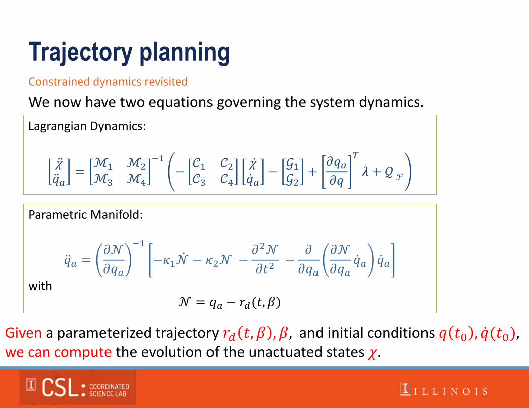
Trajectory planning Constrained dynamics revisited

Parametric Manifold:

𝑞 𝑎 =𝜕𝒩

𝜕𝑞𝑎

−1

−𝜅1𝒩 − 𝜅2𝒩 −𝜕2𝒩

𝜕𝑡2 −

𝜕

𝜕𝑞𝑎

𝜕𝒩

𝜕𝑞𝑎𝑞 𝑎 𝑞 𝑎

with 𝒩 = 𝑞𝑎 − 𝑟𝑑(𝑡, 𝛽)

We now have two equations governing the system dynamics.

Lagrangian Dynamics:

𝜒 𝑞 𝑎

=ℳ1 ℳ2

ℳ3 ℳ4

−1

−𝒞1 𝒞2𝒞3 𝒞4

𝜒 𝑞 𝑎

−𝒢1𝒢2

+𝜕𝑞𝑎𝜕𝑞

𝑇

𝜆 + 𝒬 ℱ

Given a parameterized trajectory 𝑟𝑑 𝑡, 𝛽 , 𝛽, and initial conditions 𝑞 𝑡0 , 𝑞 (𝑡0), we can compute the evolution of the unactuated states 𝜒.

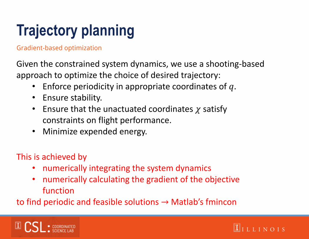
Trajectory planning Gradient-based optimization

Given the constrained system dynamics, we use a shooting-based approach to optimize the choice of desired trajectory:

• Enforce periodicity in appropriate coordinates of 𝑞. • Ensure stability. • Ensure that the unactuated coordinates 𝜒 satisfy

constraints on flight performance. • Minimize expended energy.

This is achieved by • numerically integrating the system dynamics • numerically calculating the gradient of the objective

function to find periodic and feasible solutions → Matlab’s fmincon

can be written as

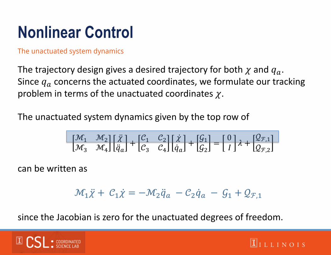
ℳ1𝜒 + 𝒞1𝜒 = −ℳ2𝑞 𝑎 − 𝒞2𝑞 𝑎 − 𝒢1 + 𝒬ℱ,1 since the Jacobian is zero for the unactuated degrees of freedom.

The unactuated system dynamics given by the top row of

ℳ1 ℳ2

ℳ3 ℳ4

𝜒 𝑞 𝑎

+𝒞1 𝒞2𝒞3 𝒞4

𝜒 𝑞 𝑎

+𝒢1𝒢2

= 0 𝐼

𝜆 +𝒬ℱ,1𝒬ℱ,2

Nonlinear Control The unactuated system dynamics

The trajectory design gives a desired trajectory for both 𝜒 and 𝑞𝑎. Since 𝑞𝑎 concerns the actuated coordinates, we formulate our tracking problem in terms of the unactuated coordinates 𝜒.

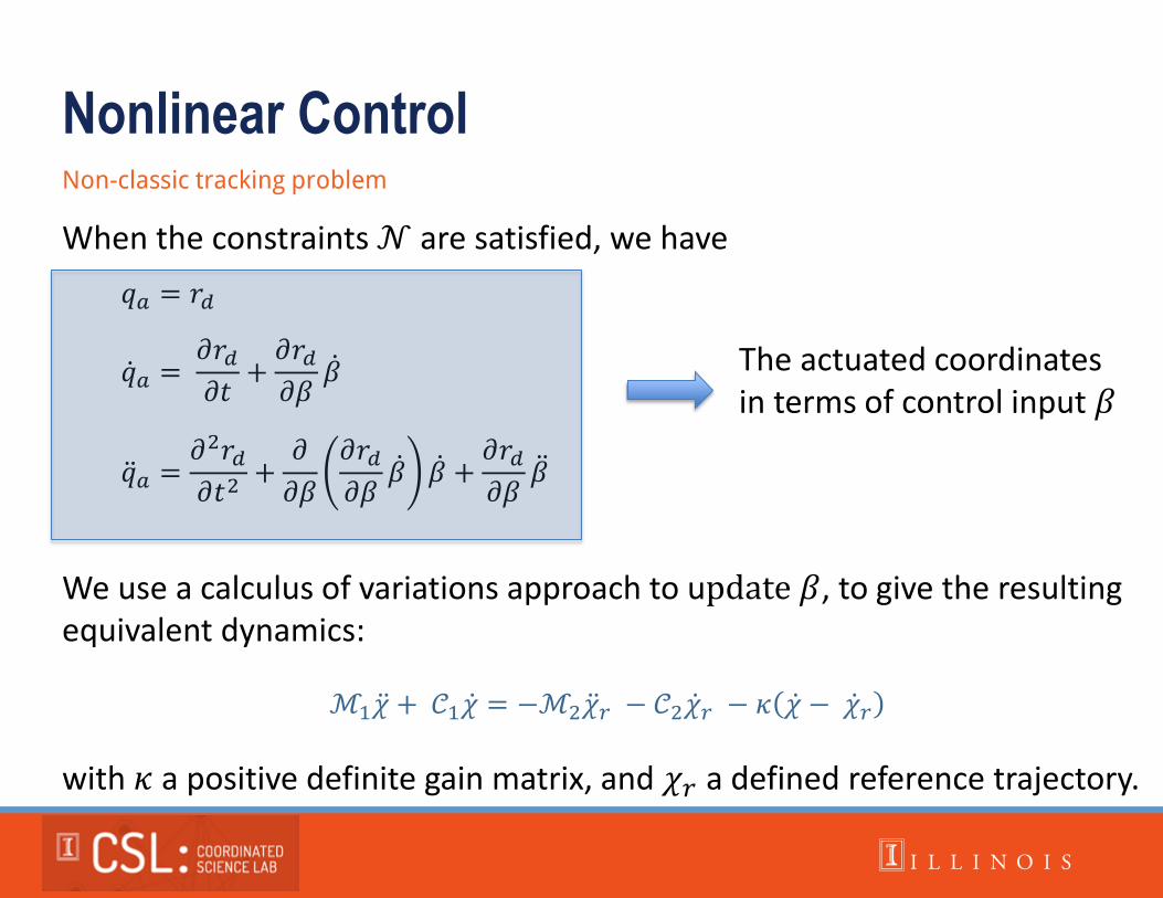
Nonlinear Control Non-classic tracking problem

When the constraints 𝒩 are satisfied, we have

𝑞 𝑎 = 𝜕𝑟𝑑𝜕𝑡

+𝜕𝑟𝑑𝜕𝛽

𝛽

𝑞 𝑎 =𝜕2𝑟𝑑𝜕𝑡2

+𝜕

𝜕𝛽

𝜕𝑟𝑑𝜕𝛽

𝛽 𝛽 +𝜕𝑟𝑑𝜕𝛽

𝛽

𝑞𝑎 = 𝑟𝑑

We use a calculus of variations approach to update 𝛽, to give the resulting equivalent dynamics:

ℳ1𝜒 + 𝒞1𝜒 = −ℳ2𝜒 𝑟 − 𝒞2𝜒 𝑟 − 𝜅 𝜒 − 𝜒 𝑟

with 𝜅 a positive definite gain matrix, and 𝜒𝑟 a defined reference trajectory.

The actuated coordinates in terms of control input 𝛽

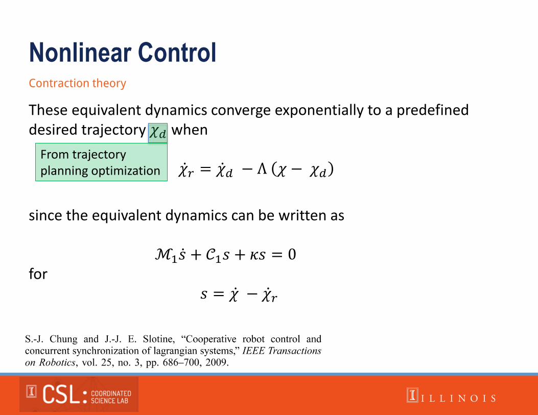
Nonlinear Control Contraction theory

These equivalent dynamics converge exponentially to a predefined desired trajectory 𝜒𝑑 when

𝜒 𝑟 = 𝜒 𝑑 − Λ 𝜒 − 𝜒𝑑

since the equivalent dynamics can be written as

ℳ1𝑠 + 𝒞1𝑠 + 𝜅𝑠 = 0 for

𝑠 = 𝜒 − 𝜒 𝑟

From trajectory planning optimization

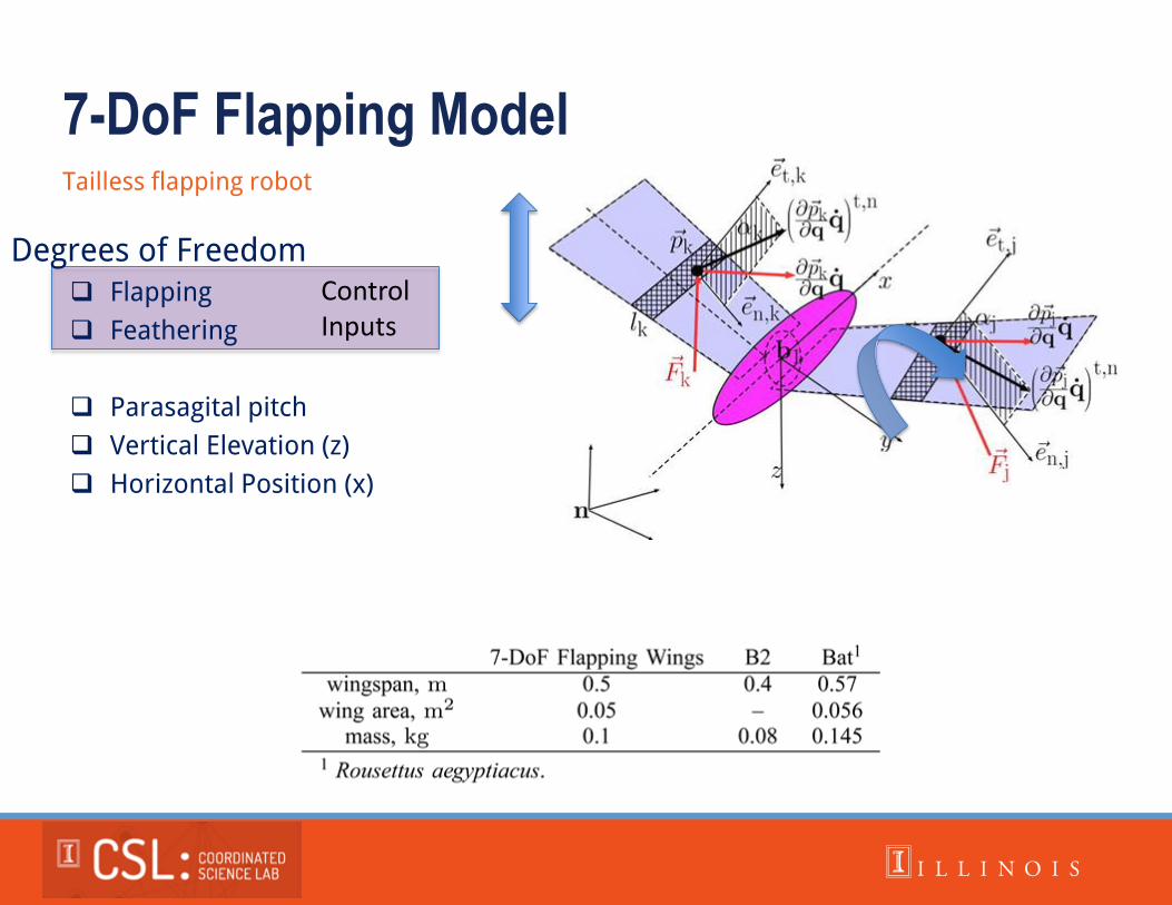
7-DoF Flapping Model Tailless flapping robot

Degrees of Freedom Flapping

Feathering

Parasagital pitch

Vertical Elevation (z)

Horizontal Position (x)

Control Inputs

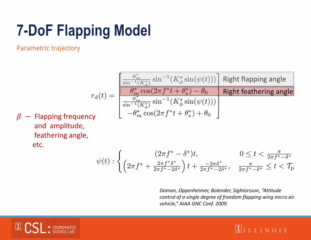
Right flapping angle

7-DoF Flapping Model Parametric trajectory

Doman, Oppenheimer, Bolender, Sightorsson, “Attitude control of a single degree of freedom flapping wing micro air vehicle,” AIAA GNC Conf. 2009.

𝛽 − Flapping frequency and amplitude, feathering angle, etc.

Right feathering angle

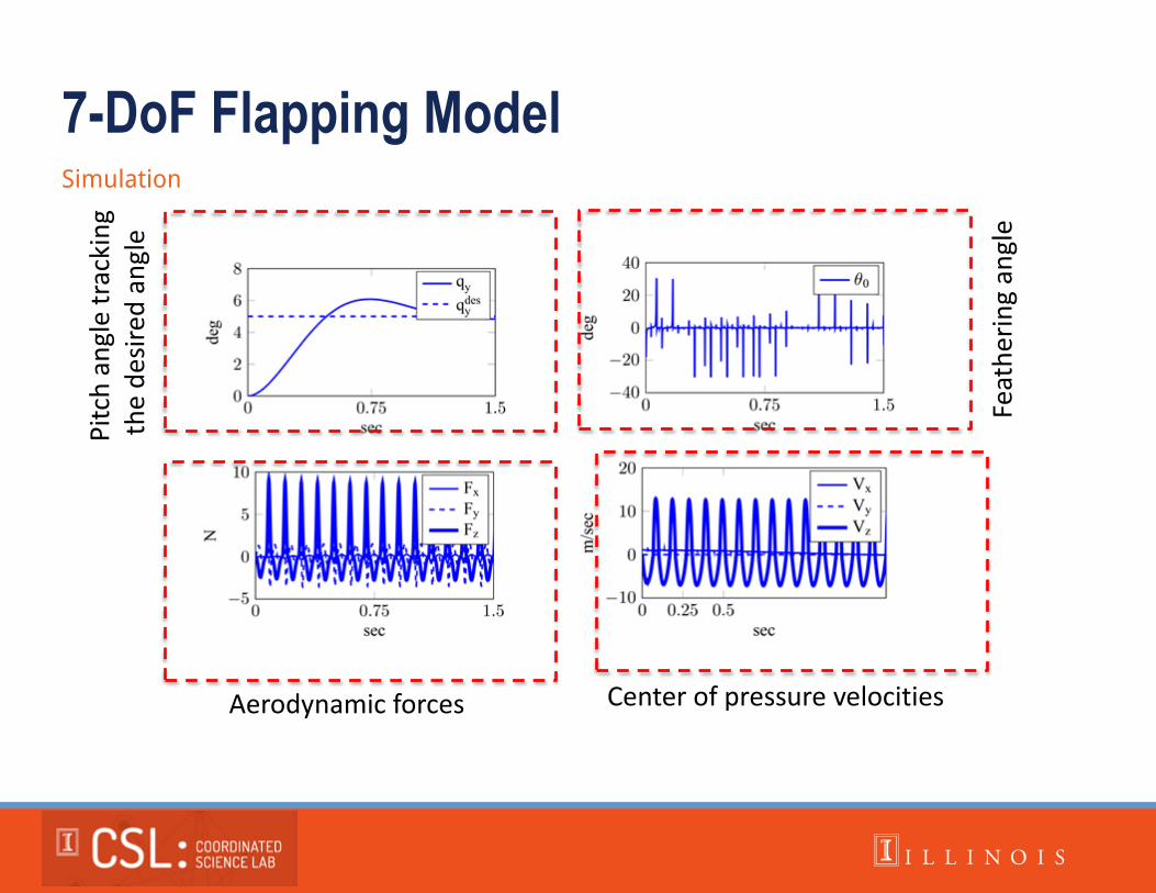
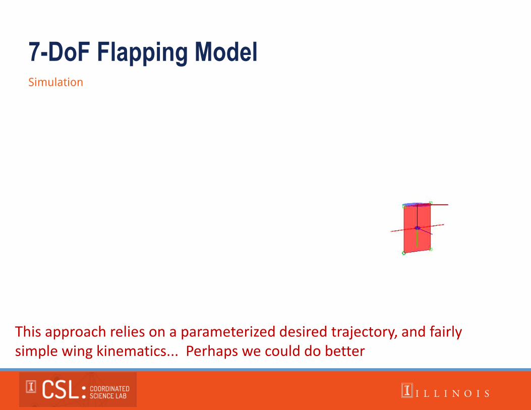
7-DoF Flapping Model Simulation

Pit

ch a

ngl

e tr

acki

ng

th

e d

esir

ed a

ngl

e

Feat

her

ing

angl

e

Aerodynamic forces Center of pressure velocities

7-DoF Flapping Model Simulation

This approach relies on a parameterized desired trajectory, and fairly simple wing kinematics... Perhaps we could do better

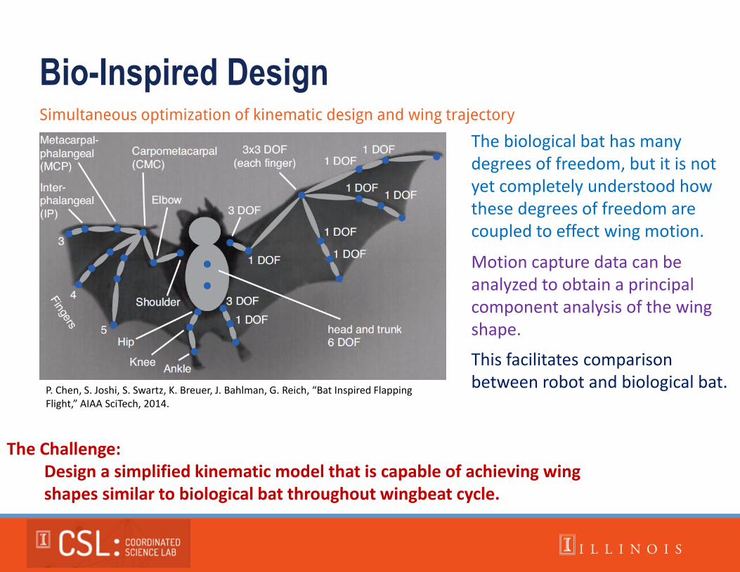
Bio-Inspired Design Simultaneous optimization of kinematic design and wing trajectory

The Challenge: Design a simplified kinematic model that is capable of achieving wing shapes similar to biological bat throughout wingbeat cycle.

The biological bat has many degrees of freedom, but it is not yet completely understood how these degrees of freedom are coupled to effect wing motion.

Motion capture data can be analyzed to obtain a principal component analysis of the wing shape.

This facilitates comparison between robot and biological bat.

P. Chen, S. Joshi, S. Swartz, K. Breuer, J. Bahlman, G. Reich, “Bat Inspired Flapping Flight,” AIAA SciTech, 2014.

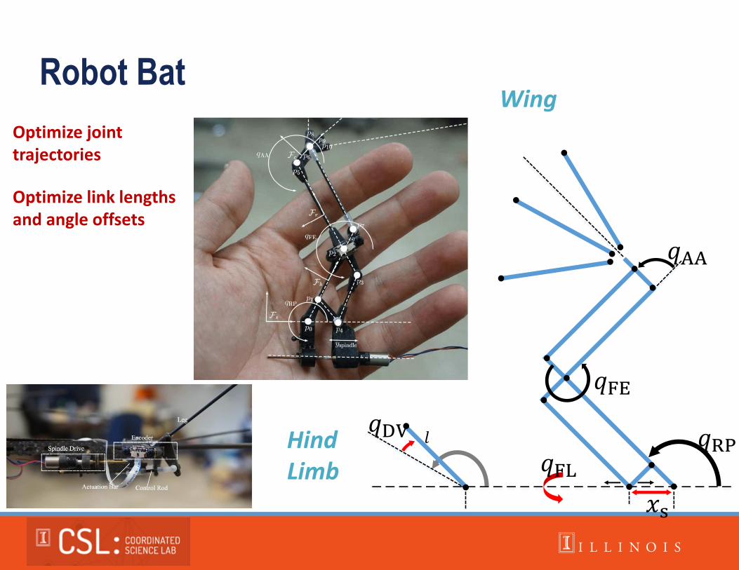
𝑞RP

𝑞FE

𝑞AA

𝑞DV

𝑥s

𝑞FL 𝑙

Optimize link lengths and angle offsets

Robot Bat

Hind Limb

Wing Optimize joint trajectories

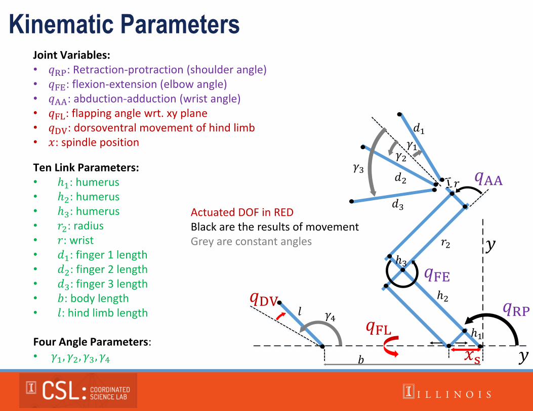
Kinematic Parameters

𝑞RP

𝑞FE

𝑞AA

𝑞DV

𝑥s

𝑞FL

𝛾1 𝛾2

𝛾3

𝛾4

ℎ1

ℎ2

ℎ3

𝑟2

𝑑1

𝑑2

𝑑3

𝑟

𝑙

𝑏

𝑦

𝑦

Actuated DOF in RED Black are the results of movement Grey are constant angles

Joint Variables: • 𝑞RP: Retraction-protraction (shoulder angle) • 𝑞FE: flexion-extension (elbow angle) • 𝑞AA: abduction-adduction (wrist angle) • 𝑞FL: flapping angle wrt. xy plane • 𝑞DV: dorsoventral movement of hind limb • 𝑥: spindle position

Ten Link Parameters: • ℎ1: humerus • ℎ2: humerus • ℎ3: humerus • 𝑟2: radius • 𝑟: wrist • 𝑑1: finger 1 length • 𝑑2: finger 2 length • 𝑑3: finger 3 length • 𝑏: body length • 𝑙: hind limb length

Four Angle Parameters: • 𝛾1, 𝛾2, 𝛾3, 𝛾4

Optimization Iterative optimization of flapping parameters and kinematic parameters

Iteratively optimize

flapping angle trajectory

spindle trajectory

link lengths and offset angles

hind limb trajectory

Optimization Criteria:

• Minimize Euclidean distance between selected makers on the biological bat and the corresponding locations on the robot bat.

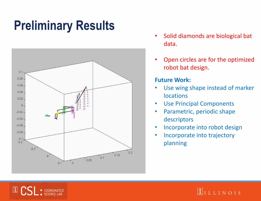
Preliminary Results • Solid diamonds are biological bat

data.

• Open circles are for the optimized robot bat design.

Future Work: • Use wing shape instead of marker

locations • Use Principal Components • Parametric, periodic shape

descriptors • Incorporate into robot design • Incorporate into trajectory

planning

Concluding Remarks

Kinematic design – passive and active joints

Nonlinear dynamics – many unactuated degrees of freedom

Actuated degrees of freedom define a manifold on which the system dynamics evolve

Design actuator inputs to define this manifold, which shapes the system dynamics

Design a nonlinear control to track the desired unactuated dynamics

Preliminary results on 7 dof simulation

Simultaneous kinematics/trajectory design

Undergraduate Researchers

Graduate Researchers

Principal Investigators Postdoc