Some 2015 Updates to the TC16 DMT Report 2001

Silvano Marchetti University of L'Aquila, Italy. E-mail: silvano@marchetti-dmt.it

Keywords:DMT, SDMT

ABSTRACT : Aims of this paper are (a) To give, at least in part, an overview of the DMT and SDMT developments in the period 2001-2015 (b) Illustrate specific aspects emerged in the years during the use and interpretation of the test (c) Possibly clarify questions that from time to time have arisen during the application of the test to the soil characterization and to the design of geotechnical works. More and more in the years has emerged the centrality of the parameter KD, one of the few in situ parameters able to provide information on stress history, whose knowledge is fundamental for obtaining reasonable predictions of settlements and liquefaction resistance.

LITERATURE ON DMT / SDMT

A considerable amount of literature concerning DMT and SDMT is available today. A list of basic DMT references, key papers, Standards, Proceedings can be found in the TC16 DMT Report 2001 (this Report is re-included as Appendix A in the Proceedings of this DMT'15 Conference).

In the last 15 years many papers on DMT and SDMT have also been published in a variety of Journals and Conferences, in particular in the Proceedings of the International Soil Characterization Conferences : ISC1 Atlanta 1998, ISC2 Porto 2004, ISC3 Taiwan 2008, ISC4 Recife 2012. Many of the key papers can be downloaded from the website : www.marchetti-dmt.it

The TC16 DMT Report 2001 and the present 2015 update represent an effort to bring together key information - including recent developments - on execution, interpretation, applications, possibly to save time to the interested reader.

INDEX

1. Current trends and ongoing developments 2. Sensitivity of DMT and CPT to Stress History 3. OCR in sand 4. K0 and Ø in sand 5. Niche of silts. Partial drainage 6. Roots of the OCR and Cu correlations 7. Displaying the DMT results 8. Similarity between KD and fs 9. Normalization exponent for KD 10. Settlements 11. Monitoring compaction

12. Go/MDMT vs (KD, ID) and Vs prediction 13. Cementation 14. Liquefaction

14.1 CRR by CPT 14.2 CRR by DMT 14.3 CRR by CPT and DMT combined 14.4 CRR from Vs (SDMT) 14.5 State parameter

15. DMT execution in semiliquid soils 16. MIX

16.1 G-gamma decay curves 16.2 Intercorrelations CPT-DMT 16.3 Reliability of ID 16.4 Advancing speed 16.5 Tip resistance Qc vs Qd 16.6 Reason of the 1.1 mm displacement 16.7 Cu field vane 16.8 Non textbook soils

1 CURRENT TRENDS AND ONGOING DEVELOPMENTS

The last decades have seen a massive migration from laboratory testing to insitu testing. Often today CPT and DMT are used as the major part of an investigation. In situ testing are fast, economical, reproducible, informative, provide many data, cost much less than sampling & testing. CPT and DMT represent a mutation compared with SPT, because the instrumental accuracy of CPT and DMT is “laboratory-grade”, unlike SPT. In situ tests are particularly helpful in sand (but also in tailings, semiliquid soils etc.) where recovering samples is difficult. In situ tests, in these materials, are the state-of-practice. It must be kept in mind, however,

that laboratory remains fundamental for research, including understanding and advancing in situ tests.

While in the laboratory "pure" soil properties such as strength, stiffness, stress history etc. can be determined, in the field it is possible to measure only "mixed" soil responses, i.e. responses that depend at the same time on strength, stiffness, stress history etc. Hence pure soil properties from in situ tests can only be obtained by "triangulation", i.e. derived by several independent in situ responses.

In the recent decades specialists of numerical models have developed a variety of constitutive models, often requiring a two-digit number of soil properties, the majority determined in the laboratory. When only in situ test results are available, the number of soil responses is dramatically lower. Yet at least several in situ responses are necessary, because the soil has many unknowns. Only in simple problems DMT alone or CPT alone may be sufficient. E.g. for predicting settlements DMT alone may be sufficient, while for detecting the depth of strong layers able to support pile tips CPT alone may be sufficient. In less simple problems a soil model is necessary, in which case a sufficient number of responses from in situ testing must be available.

When CPT and DMT are executed in sand, three independent significant parameters are obtained : Qcn, KD, ED 1 (ED1 = ED / 'vo). If SCPT or SDMT are used, then the additional parameter Vs (or Go) is obtained. An ideal future scenario could be : (a) Model specialists developing soil models based on Qcn, KD, ED1, (Go) (b) Practitioners using FEM programs by entering, for each element of the mesh, the Qcn, KD, ED1 (Go) they have measured unequivocally in situ. Moving towards an insitu

multiparameter approach appears a logical trend. It may be noted that in the above list ID and fs are

missing. However ID is known once KD and ED are known, being ID = ED /(34.7 KD 'vo). As to fs, the information contained in fs is already contained, in a more direct form, in KD, as explained in section 8.

The following example demonstrates the necessity of a multiparameter approach. In order to estimate OCR in sand both Qcn and KD are needed, i.e. CPT alone or DMT alone are insufficient. Fig. 1 by Lee et al. (2011) shows the results of a calibration chamber study comparing the reactivity to OCR of Qcn and KD in sands of various Dr. Fig. 1(a) shows that Qcn is scarcely sensitive to OCR, indicating that estimating OCR from just Qcn is problematic. Fig. 1 (b) shows that a given value of KD can be due to a low Dr and a high OCR or to a high Dr and a low OCR. In order to separate the Dr effect from the OCR effect, i.e. to pinpoint the right (OCR, Dr) pair and therefore, to estimate OCR, Qcn is also necessary to provide an indication of Dr in the horizontal axis. (preferred methods for estimating OCR in sand are covered in Section 3).

In general, for the geotechnical characterization of a site, the main contributions that DMT can provide are information on stress history (KD) and information on stiffness (via ED or MDMT). Not many alternatives are available today to obtain information on stress history, especially in sand. Yet stress history is important, in particular for estimating settlements and liquefaction resistance. For a given value of Qcn, many KD values are possible. When KD is high, settlements are smaller, liquefaction resistance is higher and a more economical foundation can be designed.

Fig. 1. Sensitivity of CPT and DMT to Stress History (Lee et al. 2011).

2 SENSITIVITY OF DMT AND CPT TO STRESS HISTORY

Numerous researchers have observed that DMT is considerably more sensitive than CPT to stress history. The first researcher to point out the higher sensitivity of DMT to stress history was Schmertmann (1984), who found, by simple experiments, that the modulus increase due to overconsolidation, predicted by DMT "was four times the modulus increase predicted by CPT" (Note that the increase of MDMT is largely due to the increase of KD, as ED increases only slightly with stress history). Schmertmann explained the different sensitivity of DMT and CPT to stress history noting that "the cone appears to destroy a large part of the modification of the soil structure caused by the overconsolidation and it therefore measures very little of the related increase in modulus. In contrast the lower strain penetration of the DMT preserves more of the effect of overconsolidation. Using the CPT to evaluate modulus changes after ground treatments may lead to a large overestimate of the settlement".

The higher sensitivity to stress history of KD, compared with the sensitivity of Qcn (normalized cone tip resistance Qc), has been observed either in the Calibration Chamber (e.g. Jamiolkowski and Lo Presti 1998) and in the field (e.g. Schmertmann et al. 1986, Jendeby 1992, Marchetti 2010).

A comprehensive calibration chamber research project, specifically aimed at comparing the effects of stress history on CPT and DMT, was carried out in Korea (Lee et al. 2011) on Busan sand. Fig.1 compares the effects of stress history on Qcn and on KD obtained by executing CPT and DMT on normally consolidated and on overconsolidated sand specimens, previously preconsolidated to OCR in the interval 1 to 8. OCR increased Qcn by a factor

1.10 to 1.15, but increased KD by a substantially higher factor 1.30 to 2.50. The regression coefficient close to 1 in the CPT diagram in Fig. 1, for data points of all OCR values, indicated poor ability of Qcn to distinguish overconsolidated sands from normally consolidated sand.

The higher sensitivity of the DMT emerges also when monitoring compaction, which is a way of imposing stress history. Schmertmann et al. (1986), noted in a compaction job "MDMT increased much more than Qc after the ground modification work, with an average (percent increase in MDMT) / (percent increase in qc) of about 2.3".

The higher sensitivity of KD to stress history includes aging (Monaco & Schmertmann 2007, Monaco and Marchetti 2007, Jamiolkowski and Lo Presti 1998, Marchetti 2010).

In conclusion Qcn reflects essentially Dr, and only to a minor

extent stress history (see Fig. 1). KD reflects the total effect of Dr plus various

stress history effects such as aging, Ko, structure and cementation (cementation is discussed in section 13).

The capability of KD to sense stress history is important, since stress history has a significant beneficial effect on stiffness and on soil resistance to liquefaction. There are not many alternatives to KD for obtaining in situ information on stress history. On the other hand if the investigation does not provide adequate information on stress history, the benefits of stress history are not felt and therefore ignored, leading to a more expensive design.

3 OCR IN SAND

In clays the correlation OCR = (0.5 KD)1.56 provides generally reasonable estimates of OCR. In contrast, in sands, KD alone is insufficient for estimating OCR and some additional information is necessary.

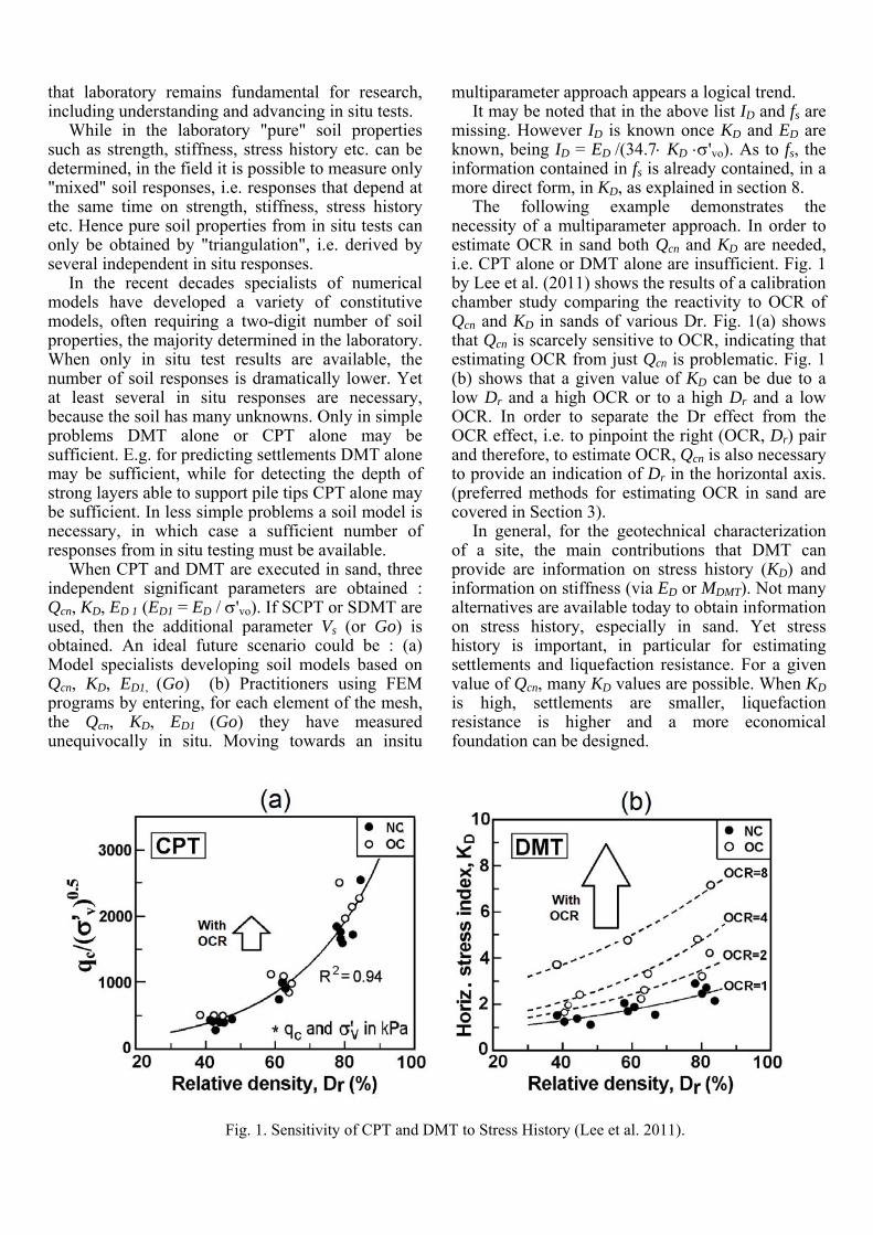
The estimation of OCR in sand was already undertaken in the TC16 DMT Report 2001, where, as a conclusion, the following semi-quantitative guidelines were given : MDMT /Qc = 5-10 in NC sands, MDMT /Qc = 12-24 in OC sands. These guidelines imply that estimating OCR in sands requires a multiparameter approach, in that both KD from DMT and Qc from CPT are needed, i.e. DMT alone or CPT alone are not sufficient. It is noted that the ratio MDMT / Qc in the above guidelines is the same ratio α = M / Qc used to get an estimate of the operative modulus.

The origin of the above guidelines is the following. In 1992 Jendeby executed DMTs and CPTs before and after the compaction of a loose

Fig. 2. Ratio MDMT /qc before/after compaction of a loose sand fill (Jendeby 1992).

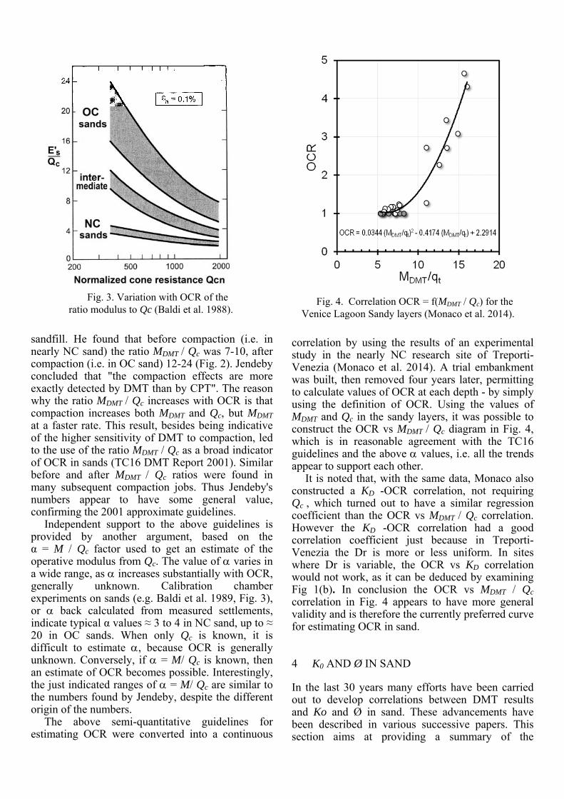
sandfill. He found that before compaction (i.e. in nearly NC sand) the ratio MDMT / Qc was 7-10, after compaction (i.e. in OC sand) 12-24 (Fig. 2). Jendeby concluded that "the compaction effects are more exactly detected by DMT than by CPT". The reason why the ratio MDMT / Qc increases with OCR is that compaction increases both MDMT and Qc, but MDMT at a faster rate. This result, besides being indicative of the higher sensitivity of DMT to compaction, led to the use of the ratio MDMT / Qc as a broad indicator of OCR in sands (TC16 DMT Report 2001). Similar before and after MDMT / Qc ratios were found in many subsequent compaction jobs. Thus Jendeby's numbers appear to have some general value, confirming the 2001 approximate guidelines.

Independent support to the above guidelines is provided by another argument, based on the α = M / Qc factor used to get an estimate of the operative modulus from Qc. The value of varies in a wide range, as increases substantially with OCR, generally unknown. Calibration chamber experiments on sands (e.g. Baldi et al. 1989, Fig. 3), or back calculated from measured settlements, indicate typical α values ≈ 3 to 4 in NC sand, up to ≈ 20 in OC sands. When only Qc is known, it is difficult to estimate , because OCR is generally unknown. Conversely, if = M/ Qc is known, then an estimate of OCR becomes possible. Interestingly, the just indicated ranges of = M/ Qc are similar to the numbers found by Jendeby, despite the different origin of the numbers.

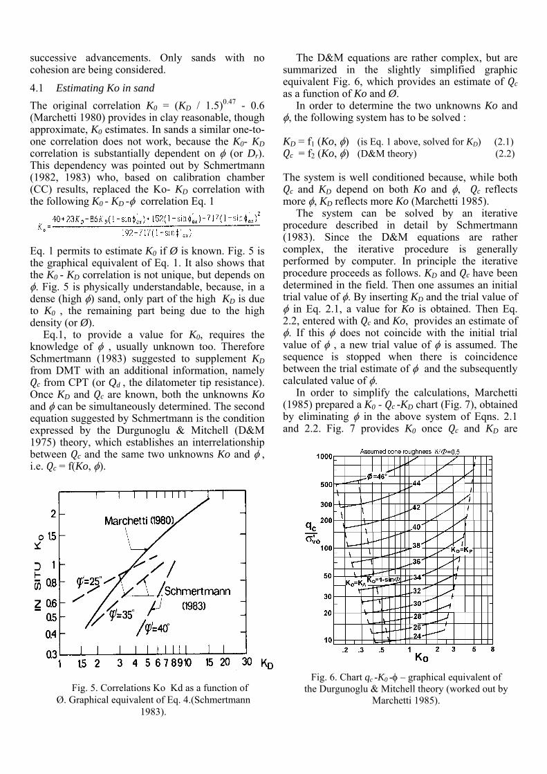
The above semi-quantitative guidelines for estimating OCR were converted into a continuous

correlation by using the results of an experimental study in the nearly NC research site of Treporti-Venezia (Monaco et al. 2014). A trial embankment was built, then removed four years later, permitting to calculate values of OCR at each depth - by simply using the definition of OCR. Using the values of MDMT and Qc in the sandy layers, it was possible to construct the OCR vs MDMT / Qc diagram in Fig. 4, which is in reasonable agreement with the TC16 guidelines and the above values, i.e. all the trends appear to support each other.

It is noted that, with the same data, Monaco also constructed a KD -OCR correlation, not requiring Qc , which turned out to have a similar regression coefficient than the OCR vs MDMT / Qc correlation. However the KD -OCR correlation had a good correlation coefficient just because in Treporti-Venezia the Dr is more or less uniform. In sites where Dr is variable, the OCR vs KD correlation would not work, as it can be deduced by examining Fig 1(b). In conclusion the OCR vs MDMT / Qc correlation in Fig. 4 appears to have more general validity and is therefore the currently preferred curve for estimating OCR in sand.

4 K0 AND Ø IN SAND

In the last 30 years many efforts have been carried out to develop correlations between DMT results and Ko and Ø in sand. These advancements have been described in various successive papers. This section aims at providing a summary of the

Fig. 4. Correlation OCR = f(MDMT / Qc) for the Venice Lagoon Sandy layers (Monaco et al. 2014).

Fig. 3. Variation with OCR of the ratio modulus to Qc (Baldi et al. 1988).

successive advancements. Only sands with no cohesion are being considered.

4.1 Estimating Ko in sand

The original correlation K0 = (KD / 1.5)0.47 - 0.6 (Marchetti 1980) provides in clay reasonable, though approximate, K0 estimates. In sands a similar one-to-one correlation does not work, because the K0- KD correlation is substantially dependent on (or Dr). This dependency was pointed out by Schmertmann (1982, 1983) who, based on calibration chamber (CC) results, replaced the Ko- KD correlation with the following K0 - KD - correlation Eq. 1 Eq. 1 permits to estimate K0 if Ø is known. Fig. 5 is the graphical equivalent of Eq. 1. It also shows that the K0 - KD correlation is not unique, but depends on . Fig. 5 is physically understandable, because, in a dense (high ) sand, only part of the high KD is due to K0 , the remaining part being due to the high density (or Ø).

Eq.1, to provide a value for K0, requires the knowledge of , usually unknown too. Therefore Schmertmann (1983) suggested to supplement KD from DMT with an additional information, namely Qc from CPT (or Qd , the dilatometer tip resistance). Once KD and Qc are known, both the unknowns Ko and can be simultaneously determined. The second equation suggested by Schmertmann is the condition expressed by the Durgunoglu & Mitchell (D&M 1975) theory, which establishes an interrelationship between Qc and the same two unknowns Ko and , i.e. Qc = f(Ko, ).

The D&M equations are rather complex, but are summarized in the slightly simplified graphic equivalent Fig. 6, which provides an estimate of Qc as a function of Ko and Ø.

In order to determine the two unknowns Ko and , the following system has to be solved : KD = f1 (Ko, ) (is Eq. 1 above, solved for KD) (2.1) Qc = f2 (Ko, ) (D&M theory) (2.2) The system is well conditioned because, while both Qc and KD depend on both Ko and , Qc reflects more , KD reflects more Ko (Marchetti 1985).

The system can be solved by an iterative procedure described in detail by Schmertmann (1983). Since the D&M equations are rather complex, the iterative procedure is generally performed by computer. In principle the iterative procedure proceeds as follows. KD and Qc have been determined in the field. Then one assumes an initial trial value of . By inserting KD and the trial value of in Eq. 2.1, a value for Ko is obtained. Then Eq. 2.2, entered with Qc and Ko, provides an estimate of . If this does not coincide with the initial trial value of , a new trial value of is assumed. The sequence is stopped when there is coincidence between the trial estimate of and the subsequently calculated value of .

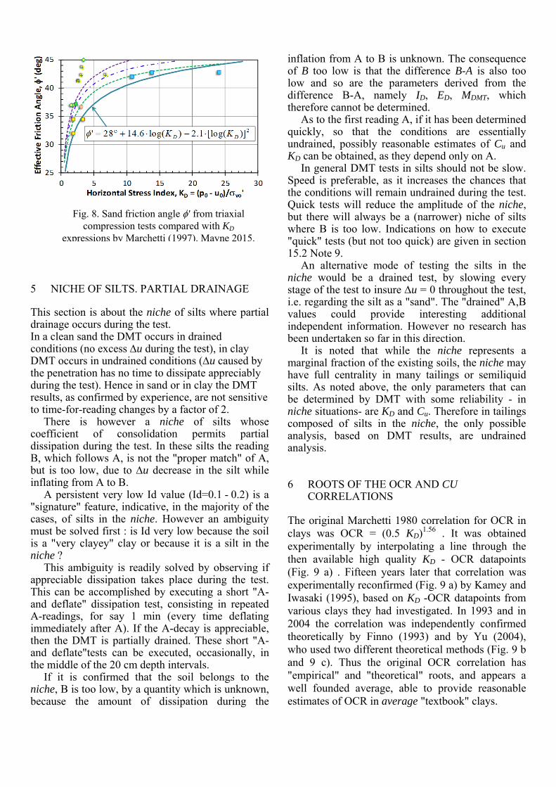
In order to simplify the calculations, Marchetti (1985) prepared a K0 - Qc -KD chart (Fig. 7), obtained by eliminating in the above system of Eqns. 2.1 and 2.2. Fig. 7 provides K0 once Qc and KD are

Fig. 5. Correlations Ko Kd as a function of Ø. Graphical equivalent of Eq. 4.(Schmertmann

1983).

Fig. 6. Chart qc -K0 - – graphical equivalent of the Durgunoglu & Mitchell theory (worked out by

Marchetti 1985).

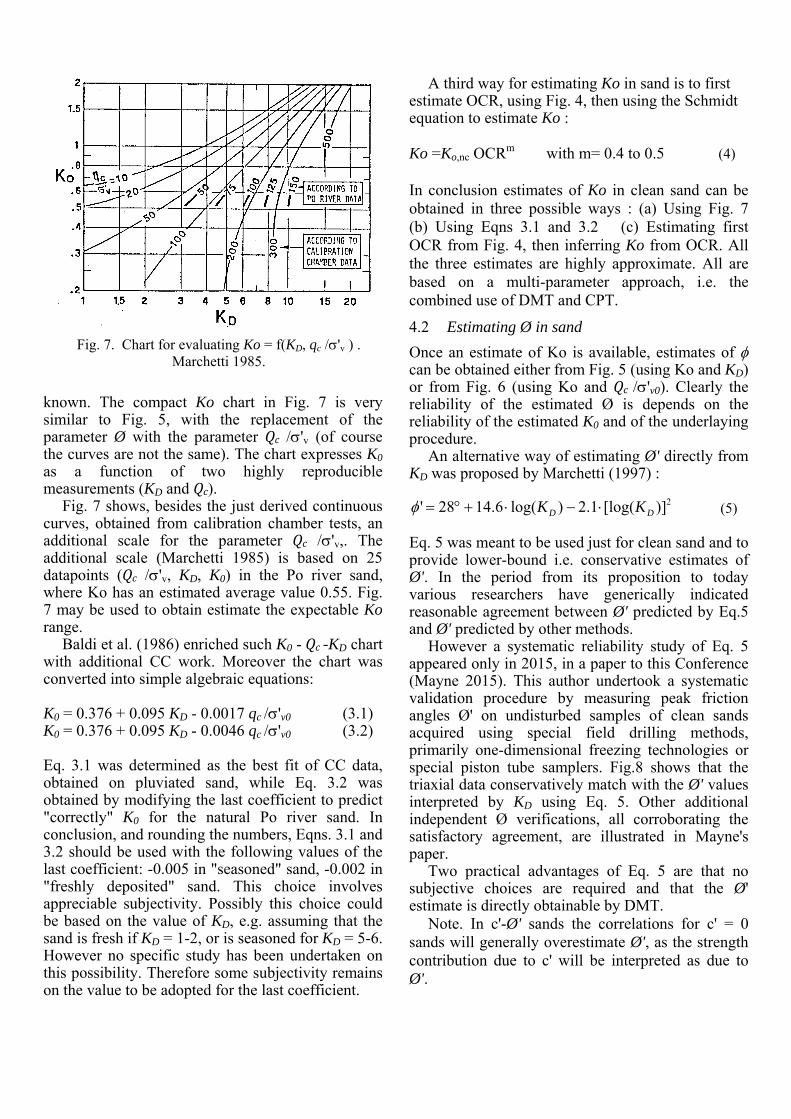
known. The compact Ko chart in Fig. 7 is very similar to Fig. 5, with the replacement of the parameter Ø with the parameter Qc /'v (of course the curves are not the same). The chart expresses K0 as a function of two highly reproducible measurements (KD and Qc).

Fig. 7 shows, besides the just derived continuous curves, obtained from calibration chamber tests, an additional scale for the parameter Qc /'v,. The additional scale (Marchetti 1985) is based on 25 datapoints (Qc /'v, KD, K0) in the Po river sand, where Ko has an estimated average value 0.55. Fig. 7 may be used to obtain estimate the expectable Ko range.

Baldi et al. (1986) enriched such K0 -Qc -KD chart with additional CC work. Moreover the chart was converted into simple algebraic equations: K0 = 0.376 + 0.095 KD - 0.0017 qc /'v0 (3.1) K0 = 0.376 + 0.095 KD - 0.0046 qc /'v0 (3.2) Eq. 3.1 was determined as the best fit of CC data, obtained on pluviated sand, while Eq. 3.2 was obtained by modifying the last coefficient to predict "correctly" K0 for the natural Po river sand. In conclusion, and rounding the numbers, Eqns. 3.1 and 3.2 should be used with the following values of the last coefficient: -0.005 in "seasoned" sand, -0.002 in "freshly deposited" sand. This choice involves appreciable subjectivity. Possibly this choice could be based on the value of KD, e.g. assuming that the sand is fresh if KD = 1-2, or is seasoned for KD = 5-6. However no specific study has been undertaken on this possibility. Therefore some subjectivity remains on the value to be adopted for the last coefficient.

A third way for estimating Ko in sand is to first estimate OCR, using Fig. 4, then using the Schmidt equation to estimate Ko : Ko =Ko,nc OCRm with m= 0.4 to 0.5 (4) In conclusion estimates of Ko in clean sand can be obtained in three possible ways : (a) Using Fig. 7 (b) Using Eqns 3.1 and 3.2 (c) Estimating first OCR from Fig. 4, then inferring Ko from OCR. All the three estimates are highly approximate. All are based on a multi-parameter approach, i.e. the combined use of DMT and CPT.

4.2 Estimating Ø in sand

Once an estimate of Ko is available, estimates of can be obtained either from Fig. 5 (using Ko and KD) or from Fig. 6 (using Ko and Qc /'v0). Clearly the reliability of the estimated Ø is depends on the reliability of the estimated K0 and of the underlaying procedure.

An alternative way of estimating Ø' directly from KD was proposed by Marchetti (1997) : (5) Eq. 5 was meant to be used just for clean sand and to provide lower-bound i.e. conservative estimates of Ø'. In the period from its proposition to today various researchers have generically indicated reasonable agreement between Ø' predicted by Eq.5 and Ø' predicted by other methods.

However a systematic reliability study of Eq. 5 appeared only in 2015, in a paper to this Conference (Mayne 2015). This author undertook a systematic validation procedure by measuring peak friction angles Ø' on undisturbed samples of clean sands acquired using special field drilling methods, primarily one-dimensional freezing technologies or special piston tube samplers. Fig.8 shows that the triaxial data conservatively match with the Ø' values interpreted by KD using Eq. 5. Other additional independent Ø verifications, all corroborating the satisfactory agreement, are illustrated in Mayne's paper.

Two practical advantages of Eq. 5 are that no subjective choices are required and that the Ø' estimate is directly obtainable by DMT.

Note. In c'-Ø' sands the correlations for c' = 0 sands will generally overestimate Ø', as the strength contribution due to c' will be interpreted as due to Ø'.

2)][log(1.2)log(6.1428' DD KK

Fig. 7. Chart for evaluating Ko = f(KD, qc /'v ) . Marchetti 1985.

5 NICHE OF SILTS. PARTIAL DRAINAGE

This section is about the niche of silts where partial drainage occurs during the test. In a clean sand the DMT occurs in drained conditions (no excess u during the test), in clay DMT occurs in undrained conditions (u caused by the penetration has no time to dissipate appreciably during the test). Hence in sand or in clay the DMT results, as confirmed by experience, are not sensitive to time-for-reading changes by a factor of 2.

There is however a niche of silts whose coefficient of consolidation permits partial dissipation during the test. In these silts the reading B, which follows A, is not the "proper match" of A, but is too low, due to u decrease in the silt while inflating from A to B.

A persistent very low Id value (Id=0.1 - 0.2) is a "signature" feature, indicative, in the majority of the cases, of silts in the niche. However an ambiguity must be solved first : is Id very low because the soil is a "very clayey" clay or because it is a silt in the niche ?

This ambiguity is readily solved by observing if appreciable dissipation takes place during the test. This can be accomplished by executing a short "A-and deflate" dissipation test, consisting in repeated A-readings, for say 1 min (every time deflating immediately after A). If the A-decay is appreciable, then the DMT is partially drained. These short "A-and deflate"tests can be executed, occasionally, in the middle of the 20 cm depth intervals.

If it is confirmed that the soil belongs to the niche, B is too low, by a quantity which is unknown, because the amount of dissipation during the

inflation from A to B is unknown. The consequence of B too low is that the difference B-A is also too low and so are the parameters derived from the difference B-A, namely ID, ED, MDMT, which therefore cannot be determined.

As to the first reading A, if it has been determined quickly, so that the conditions are essentially undrained, possibly reasonable estimates of Cu and KD can be obtained, as they depend only on A.

In general DMT tests in silts should not be slow. Speed is preferable, as it increases the chances that the conditions will remain undrained during the test. Quick tests will reduce the amplitude of the niche, but there will always be a (narrower) niche of silts where B is too low. Indications on how to execute "quick" tests (but not too quick) are given in section 15.2 Note 9.

An alternative mode of testing the silts in the niche would be a drained test, by slowing every stage of the test to insure u = 0 throughout the test, i.e. regarding the silt as a "sand". The "drained" A,B values could provide interesting additional independent information. However no research has been undertaken so far in this direction.

It is noted that while the niche represents a marginal fraction of the existing soils, the niche may have full centrality in many tailings or semiliquid silts. As noted above, the only parameters that can be determined by DMT with some reliability - in niche situations- are KD and Cu. Therefore in tailings composed of silts in the niche, the only possible analysis, based on DMT results, are undrained analysis.

6 ROOTS OF THE OCR AND CU CORRELATIONS

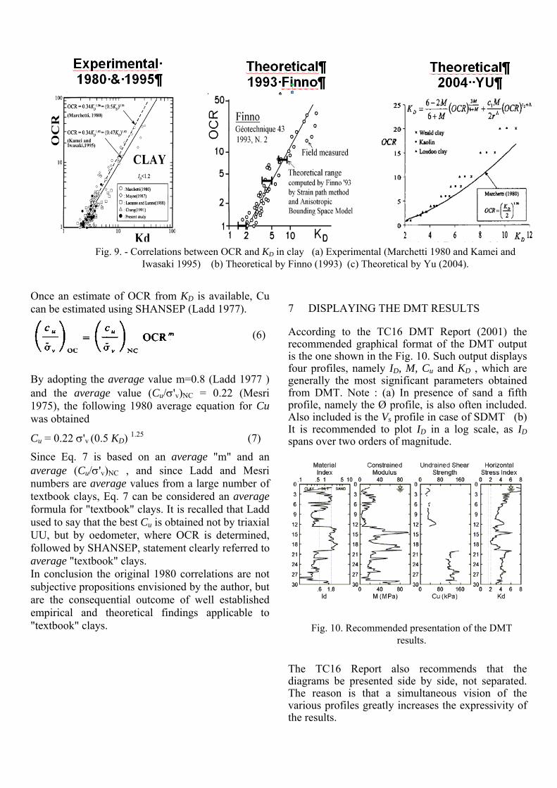
The original Marchetti 1980 correlation for OCR in clays was OCR = (0.5 KD)1.56 . It was obtained experimentally by interpolating a line through the then available high quality KD - OCR datapoints (Fig. 9 a) . Fifteen years later that correlation was experimentally reconfirmed (Fig. 9 a) by Kamey and Iwasaki (1995), based on KD -OCR datapoints from various clays they had investigated. In 1993 and in 2004 the correlation was independently confirmed theoretically by Finno (1993) and by Yu (2004), who used two different theoretical methods (Fig. 9 b and 9 c). Thus the original OCR correlation has "empirical" and "theoretical" roots, and appears a well founded average, able to provide reasonable estimates of OCR in average "textbook" clays.

Fig. 8. Sand friction angle ' from triaxial compression tests compared with KD

expressions by Marchetti (1997). Mayne 2015.

Once an estimate of OCR from KD is available, Cu can be estimated using SHANSEP (Ladd 1977). (6)

By adopting the average value m=0.8 (Ladd 1977 ) and the average value (Cu/'v)NC = 0.22 (Mesri 1975), the following 1980 average equation for Cu was obtained

Cu = 0.22 'v (0.5 KD) 1.25 (7)

Since Eq. 7 is based on an average "m" and an average (Cu/'v)NC , and since Ladd and Mesri numbers are average values from a large number of textbook clays, Eq. 7 can be considered an average formula for "textbook" clays. It is recalled that Ladd used to say that the best Cu is obtained not by triaxial UU, but by oedometer, where OCR is determined, followed by SHANSEP, statement clearly referred to average "textbook" clays. In conclusion the original 1980 correlations are not subjective propositions envisioned by the author, but are the consequential outcome of well established empirical and theoretical findings applicable to "textbook" clays.

7 DISPLAYING THE DMT RESULTS

According to the TC16 DMT Report (2001) the recommended graphical format of the DMT output is the one shown in the Fig. 10. Such output displays four profiles, namely ID, M, Cu and KD , which are generally the most significant parameters obtained from DMT. Note : (a) In presence of sand a fifth profile, namely the Ø profile, is also often included. Also included is the Vs profile in case of SDMT (b) It is recommended to plot ID in a log scale, as ID spans over two orders of magnitude.

The TC16 Report also recommends that the diagrams be presented side by side, not separated. The reason is that a simultaneous vision of the various profiles greatly increases the expressivity of the results.

Fig. 9. - Correlations between OCR and KD in clay (a) Experimental (Marchetti 1980 and Kamei and Iwasaki 1995) (b) Theoretical by Finno (1993) (c) Theoretical by Yu (2004).

Fig. 10. Recommended presentation of the DMT results.

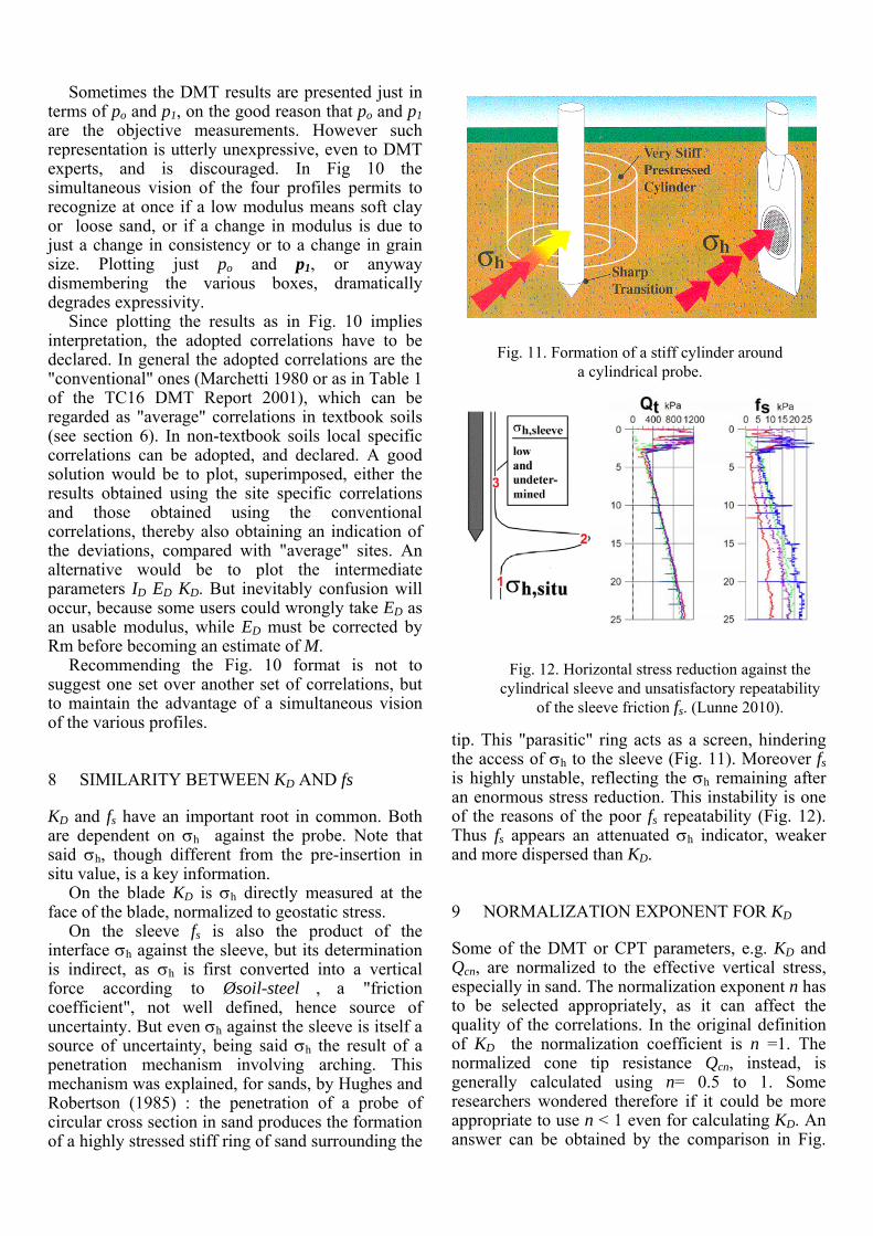
Sometimes the DMT results are presented just in terms of po and p1, on the good reason that po and p1 are the objective measurements. However such representation is utterly unexpressive, even to DMT experts, and is discouraged. In Fig 10 the simultaneous vision of the four profiles permits to recognize at once if a low modulus means soft clay or loose sand, or if a change in modulus is due to just a change in consistency or to a change in grain size. Plotting just po and p1, or anyway dismembering the various boxes, dramatically degrades expressivity.

Since plotting the results as in Fig. 10 implies interpretation, the adopted correlations have to be declared. In general the adopted correlations are the "conventional" ones (Marchetti 1980 or as in Table 1 of the TC16 DMT Report 2001), which can be regarded as "average" correlations in textbook soils (see section 6). In non-textbook soils local specific correlations can be adopted, and declared. A good solution would be to plot, superimposed, either the results obtained using the site specific correlations and those obtained using the conventional correlations, thereby also obtaining an indication of the deviations, compared with "average" sites. An alternative would be to plot the intermediate parameters ID ED KD. But inevitably confusion will occur, because some users could wrongly take ED as an usable modulus, while ED must be corrected by Rm before becoming an estimate of M.

Recommending the Fig. 10 format is not to suggest one set over another set of correlations, but to maintain the advantage of a simultaneous vision of the various profiles.

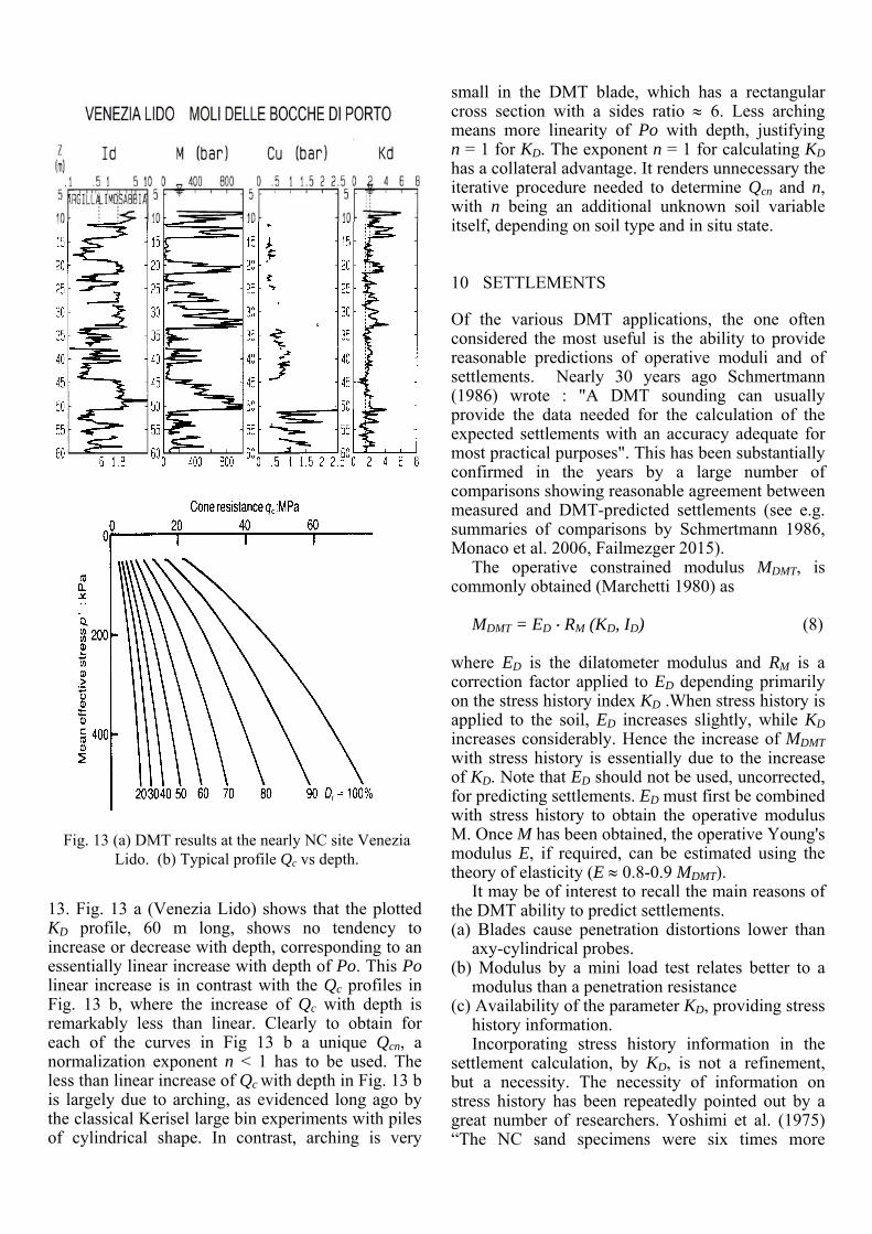
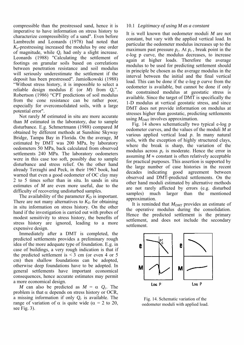
8 SIMILARITY BETWEEN KD AND fs

KD and fs have an important root in common. Both are dependent on h against the probe. Note that said h, though different from the pre-insertion in situ value, is a key information.

On the blade KD is h directly measured at the face of the blade, normalized to geostatic stress.

On the sleeve fs is also the product of the interface h against the sleeve, but its determination is indirect, as h is first converted into a vertical force according to Øsoil-steel , a "friction coefficient", not well defined, hence source of uncertainty. But even h against the sleeve is itself a source of uncertainty, being said h the result of a penetration mechanism involving arching. This mechanism was explained, for sands, by Hughes and Robertson (1985) : the penetration of a probe of circular cross section in sand produces the formation of a highly stressed stiff ring of sand surrounding the

tip. This "parasitic" ring acts as a screen, hindering the access of h to the sleeve (Fig. 11). Moreover fs is highly unstable, reflecting the h remaining after an enormous stress reduction. This instability is one of the reasons of the poor fs repeatability (Fig. 12). Thus fs appears an attenuated h indicator, weaker and more dispersed than KD.

9 NORMALIZATION EXPONENT FOR KD

Some of the DMT or CPT parameters, e.g. KD and Qcn, are normalized to the effective vertical stress, especially in sand. The normalization exponent n has to be selected appropriately, as it can affect the quality of the correlations. In the original definition of KD the normalization coefficient is n =1. The normalized cone tip resistance Qcn, instead, is generally calculated using n= 0.5 to 1. Some researchers wondered therefore if it could be more appropriate to use n < 1 even for calculating KD. An answer can be obtained by the comparison in Fig.

Fig. 11. Formation of a stiff cylinder around a cylindrical probe.

Fig. 12. Horizontal stress reduction against the cylindrical sleeve and unsatisfactory repeatability

of the sleeve friction fs. (Lunne 2010).

13. Fig. 13 a (Venezia Lido) shows that the plotted KD profile, 60 m long, shows no tendency to increase or decrease with depth, corresponding to an essentially linear increase with depth of Po. This Po linear increase is in contrast with the Qc profiles in Fig. 13 b, where the increase of Qc with depth is remarkably less than linear. Clearly to obtain for each of the curves in Fig 13 b a unique Qcn, a normalization exponent n < 1 has to be used. The less than linear increase of Qc with depth in Fig. 13 b is largely due to arching, as evidenced long ago by the classical Kerisel large bin experiments with piles of cylindrical shape. In contrast, arching is very

small in the DMT blade, which has a rectangular cross section with a sides ratio 6. Less arching means more linearity of Po with depth, justifying n = 1 for KD. The exponent n = 1 for calculating KD has a collateral advantage. It renders unnecessary the iterative procedure needed to determine Qcn and n, with n being an additional unknown soil variable itself, depending on soil type and in situ state.

10 SETTLEMENTS

Of the various DMT applications, the one often considered the most useful is the ability to provide reasonable predictions of operative moduli and of settlements. Nearly 30 years ago Schmertmann (1986) wrote : "A DMT sounding can usually provide the data needed for the calculation of the expected settlements with an accuracy adequate for most practical purposes". This has been substantially confirmed in the years by a large number of comparisons showing reasonable agreement between measured and DMT-predicted settlements (see e.g. summaries of comparisons by Schmertmann 1986, Monaco et al. 2006, Failmezger 2015).

The operative constrained modulus MDMT, is commonly obtained (Marchetti 1980) as

MDMT = ED RM (KD, ID) (8)

where ED is the dilatometer modulus and RM is a correction factor applied to ED depending primarily on the stress history index KD .When stress history is applied to the soil, ED increases slightly, while KD increases considerably. Hence the increase of MDMT with stress history is essentially due to the increase of KD. Note that ED should not be used, uncorrected, for predicting settlements. ED must first be combined with stress history to obtain the operative modulus M. Once M has been obtained, the operative Young's modulus E, if required, can be estimated using the theory of elasticity (E 0.8-0.9 MDMT).

It may be of interest to recall the main reasons of the DMT ability to predict settlements. (a) Blades cause penetration distortions lower than

axy-cylindrical probes. (b) Modulus by a mini load test relates better to a

modulus than a penetration resistance (c) Availability of the parameter KD, providing stress

history information. Incorporating stress history information in the

settlement calculation, by KD, is not a refinement, but a necessity. The necessity of information on stress history has been repeatedly pointed out by a great number of researchers. Yoshimi et al. (1975) “The NC sand specimens were six times more

Fig. 13 (a) DMT results at the nearly NC site Venezia Lido. (b) Typical profile Qc vs depth.

compressible than the prestressed sand, hence it is imperative to have information on stress history to characterize compressibility of a sand". Even before Lambrecht and Leonards (1978) had noted that Ko-prestressing increased the modulus by one order of magnitude, while Qc had only a slight increase. Leonards (1988) "Calculating the settlement of footings on granular soils based on correlations between penetration resistance and soil modulus will seriously underestimate the settlement if the deposit has been prestressed". Jamiolkowski (1988) “Without stress history, it is impossible to select a reliable design modulus E (or M) from Qc”. Robertson (1986) “CPT predictions of soil modulus from the cone resistance can be rather poor, especially for overconsolidated soils, with a large potential error".

Not rarely M estimated in situ are more accurate than M estimated in the laboratory, due to sample disturbance. E.g. Schmertmann (1988) compared M obtained by different methods at Sunshine Skyway Bridge, Tampa Bay in Florida. On the average, M estimated by DMT was 200 MPa, by laboratory oedometers 50 MPa, back calculated from observed settlements 240 MPa. The laboratory oedometers were in this case too soft, possibly due to sample disturbance and stress relief. On the other hand already Terzaghi and Peck, in their 1967 book, had warned that even a good oedometer of OC clay may 2 to 5 times softer than in situ. In sands in situ estimates of M are even more useful, due to the difficulty of recovering undisturbed samples.

The availability of the parameter KD is important. There are not many alternatives to KD for obtaining in situ information on stress history. On the other hand if the investigation is carried out with probes of modest sensitivity to stress history, the benefits of stress history are ignored, leading to a more expensive design.

Immediately after a DMT is completed, the predicted settlements provides a preliminary rough idea of the more adequate type of foundation. E.g. in case of buildings, a very rough indication is that if the predicted settlement is < 3 cm (or even 4 or 5 cm) then shallow foundations can be adopted, otherwise deep foundations have to be adopted. In general settlements have important economical consequences, hence accurate estimates may permit a more economical design.

M can also be predicted as M = Qc. The problem is that depends on stress history or OCR, a missing information if only Qc is available. The range of variation of is quite wide ( = 2 to 20, see Fig. 3).

10.1 Legitimacy of using M as a constant

It is well known that oedometer moduli M are not constant, but vary with the applied vertical load. In particular the oedometer modulus increases up to the maximum past pressure pc. At pc , break point in the e-log p curve, the modulus decreases, to increase again at higher loads. Therefore the average modulus to be used for predicting settlement should in principle be chosen as the average modulus in the interval between the initial and the final vertical load. This can be done if the e-log p curve from the oedometer is available, but cannot be done if only the constrained modulus at geostatic stress is available. Since the target of DMT is specifically the 1-D modulus at vertical geostatic stress, and since DMT does not provide information on modulus at stresses higher than geostatic, predicting settlements using MDMT involves approximation.

Fig. 14 shows schematically two typical e-log p oedometer curves, and the values of the moduli M at various applied vertical load p. In many natural soils, with the exception of highly structured clays, where the break is sharp, the variation of the modulus across pc is moderate. Hence the error in assuming M constant is often relatively acceptable for practical purposes. This assertion is supported by the large number of case histories in the recent decades indicating good agreement between observed and DMT-predicted settlements. On the other hand moduli estimated by alternative methods are not rarely affected by errors (e.g. disturbed samples) much larger than the mentioned approximation.

It is reminded that MDMT provides an estimate of the operative modulus during the consolidation. Hence the predicted settlement is the primary settlement, and does not include the secondary settlement.

Fig. 14. Schematic variation of the oedometer moduli with applied load.

10.2 Deriving M drained from an undrained test

In clay, the expansion of the membrane occurs in undrained conditions. Therefore the dilatometer modulus ED is an undrained modulus. Thus, according to logic, the correlation to be investigated should be between ED and the undrained modulus Eu. Attempts of this kind were carried out in the early days of the DMT development. However a big obstacle, precluding such possibility, was the high variability of the undrained moduli provided by different laboratories, at least in part due to the high sensitivity of Eu to the disturbance. Hence, as a second attempt, the correlation ED - M was investigated. This correlation involves many soil properties, including material type, anisotropy, pore pressure parameters etc. Hence no unique ED - M correlation can be expected. On the other hand the DMT provides, in addition to ED, also the parameters ID and KD , containing at least some information on material type and stress history. This availability provides some basis to expect at least some degree of correlation ED - M , using ID and KD as parameters. Moreover, while the correlation ED - M is, at least in principle, weaker than ED - Eu , at least ED - M can be tested, because M by different laboratory have much less variability than Eu.

Obviously the final word goes to real world observations. Large number of case histories have generally proved the favorable comparisons between observed and DMT-predicted primary settlements, thereby supporting the use of MDMT as operative constrained modulus.

Note also Lambe et al. (1977) : “Drained moduli of saturated clays are typically about one-third to one-fourth the undrained values”. Hence a broad connection drained-undrained stiffness has already been invoked in the past.

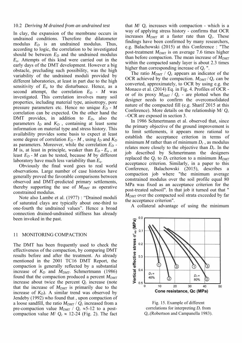
11 MONITORING COMPACTION

The DMT has been frequently used to check the effectiveness of the compaction, by comparing DMT results before and after the treatment. As already mentioned in the 2001 TC16 DMT Report, the compaction is generally reflected by a substantial increase of KD and MDMT. Schmertmann (1986) found that the compaction produced a percent MDMT increase about twice the percent Qc increase (note that the increase of MDMT is primarily due to the increase of KD). A similar trend was observed by Jendeby (1992) who found that , upon compaction of a loose sandfill, the ratio MDMT / Qc increased from a pre-compaction value MDMT / Qc 5-12 to a post-compaction value M/ Qc 12-24 (Fig. 2). The fact

that M/ Qc increases with compaction - which is a way of applying stress history - confirms that OCR increases MDMT at a faster rate than Qc. These findings have been confirmed by many researchers, e.g. Balachowski (2015) at this Conference : "The post-treatment MDMT is on average 7.6 times higher than before compaction. The mean increase of MDMT within the compacted sandy layer is about 2.3 times higher than corresponding increase of Qc ".

The ratio MDMT / Qc appears an indicator of the OCR achieved by the compaction. MDMT / Qc can be converted, approximately, to OCR by using e.g. the Monaco et al. (2014) Eq. in Fig. 4. Profiles of OCR - or of its proxy MDMT / Qc - are plotted when the designer needs to confirm the overconsolidated nature of the compacted fill (e.g. Sharif 2015 at this Conference). More details on the relationship M/ Qc

- OCR are exposed in section 3. In 1986 Schmertmann et al. observed that, since

the primary objective of the ground improvement is to limit settlements, it appears more rational to establish the acceptance criterion in terms of minimum M rather than of minimum Dr , as modulus relates more closely to the objective than Dr. In the job described by Schmertmann the designers replaced the Qc to Dr criterion to a minimum MDMT acceptance criterion. Similarly, in a paper to this Conference, Balachowski (2015), describes a compaction job where "the minimum average constrained modulus over the soil profile equal 80 MPa was fixed as an acceptance criterion for the post-treated subsoil". In that job it turned out that " MDMT over the compacted soil strata exceeded by far the acceptance criterion".

A collateral advantage of using the minimum

Fig. 15. Example of different correlations for interpreting Dr from

Qc.(Robertson and Campanella 1983).

MDMT acceptance criterion is avoiding the in situ Dr determination, often problematic. AspointedoutbyRobertson and Campanella (1983) Hilton Minessand atDr =60% has the sameQc as MontereysandatDr=40%,i.e.thereisnouniquemappingQctoDrapplicabletoallsands(Fig.15).

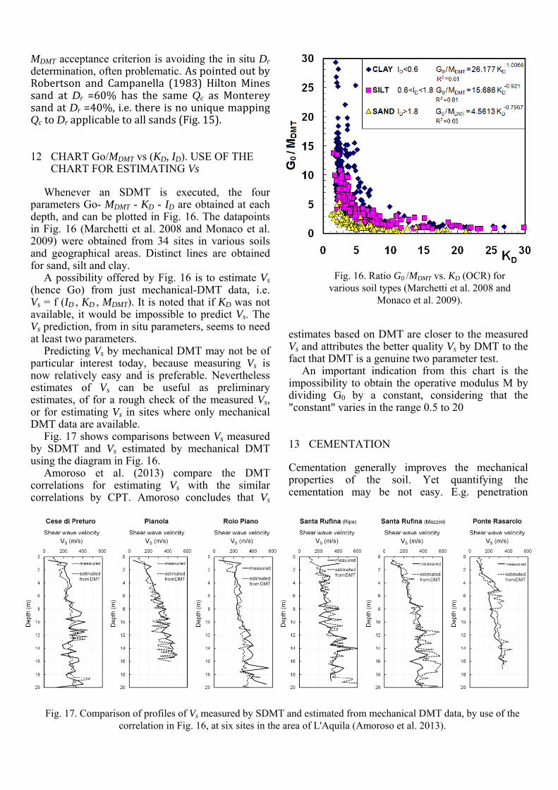
12 CHART Go/MDMT vs (KD, ID). USE OF THE CHART FOR ESTIMATING Vs

Whenever an SDMT is executed, the four parameters Go- MDMT - KD - ID are obtained at each depth, and can be plotted in Fig. 16. The datapoints in Fig. 16 (Marchetti et al. 2008 and Monaco et al. 2009) were obtained from 34 sites in various soils and geographical areas. Distinct lines are obtained for sand, silt and clay.

A possibility offered by Fig. 16 is to estimate Vs (hence Go) from just mechanical-DMT data, i.e. Vs = f (ID , KD , MDMT). It is noted that if KD was not available, it would be impossible to predict Vs. The Vs prediction, from in situ parameters, seems to need at least two parameters.

Predicting Vs by mechanical DMT may not be of particular interest today, because measuring Vs is now relatively easy and is preferable. Nevertheless estimates of Vs can be useful as preliminary estimates, of for a rough check of the measured Vs, or for estimating Vs in sites where only mechanical DMT data are available.

Fig. 17 shows comparisons between Vs measured by SDMT and Vs estimated by mechanical DMT using the diagram in Fig. 16.

Amoroso et al. (2013) compare the DMT correlations for estimating Vs with the similar correlations by CPT. Amoroso concludes that Vs

estimates based on DMT are closer to the measured Vs and attributes the better quality Vs by DMT to the fact that DMT is a genuine two parameter test.

An important indication from this chart is the impossibility to obtain the operative modulus M by dividing G0 by a constant, considering that the "constant" varies in the range 0.5 to 20

13 CEMENTATION

Cementation generally improves the mechanical properties of the soil. Yet quantifying the cementation may be not easy. E.g. penetration

Fig. 17. Comparison of profiles of Vs measured by SDMT and estimated from mechanical DMT data, by use of the correlation in Fig. 16, at six sites in the area of L'Aquila (Amoroso et al. 2013).

Fig. 16. Ratio G0 /MDMT vs. KD (OCR) for various soil types (Marchetti et al. 2008 and

Monaco et al. 2009).

probes could not feel the benefits of the cementation in a similar proportion as the soil, because the insertion may partly destroy the cementation. One factor controlling the entity of the destruction is the distortion caused by the penetration. Another factor is the nature of the cementation, that can be ductile (toothpaste-like) or fragile (glasslike). A fragile cementation is more vulnerable. Fine soils have often a ductile, less vulnerable, cementation.

One parameter that can help for investigating the cementation is KD. Experience has shown that, in clay, KD increases with cementation. E.g. higher than expected KD were observed at the Fucino site (Marchetti 1980, AGI 1991) and at S. Barbara site (Marchetti 1991), where the calcium carbonate content was particularly high. However in sands having a cementation of the fragile type the blade penetration is likely to destroy at least part of the cementation. Hence it is not warranted that in these sands KD increases with the cementation, despite that in the sand the effect is beneficial.

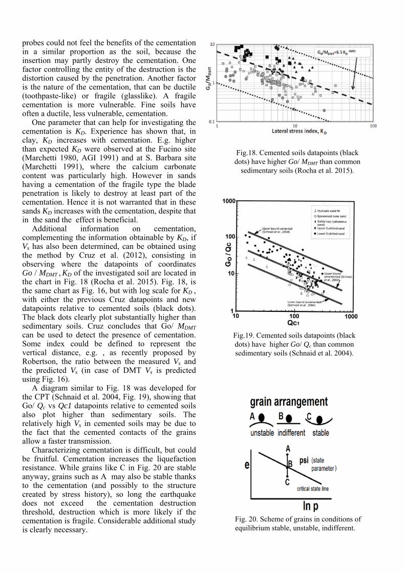
Additional information on cementation, complementing the information obtainable by KD, if Vs has also been determined, can be obtained using the method by Cruz et al. (2012), consisting in observing where the datapoints of coordinates Go / MDMT , KD of the investigated soil are located in the chart in Fig. 18 (Rocha et al. 2015). Fig. 18, is the same chart as Fig. 16, but with log scale for KD , with either the previous Cruz datapoints and new datapoints relative to cemented soils (black dots). The black dots clearly plot substantially higher than sedimentary soils. Cruz concludes that Go/ MDMT can be used to detect the presence of cementation. Some index could be defined to represent the vertical distance, e.g. , as recently proposed by Robertson, the ratio between the measured Vs and the predicted Vs (in case of DMT Vs is predicted using Fig. 16).

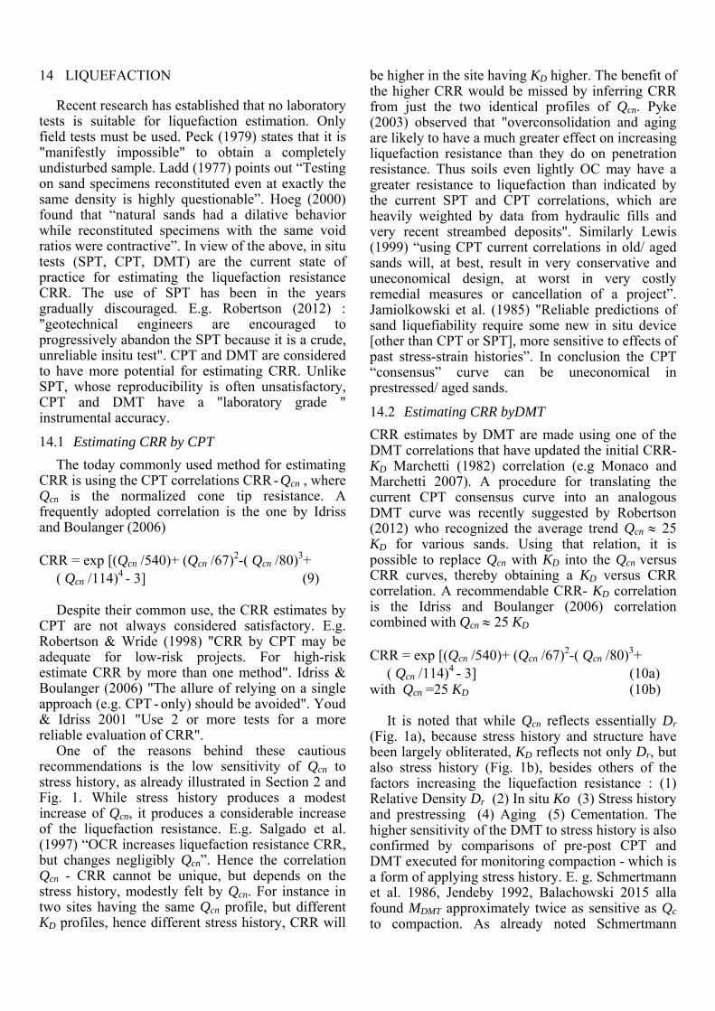
A diagram similar to Fig. 18 was developed for the CPT (Schnaid et al. 2004, Fig. 19), showing that Go/ Qc vs Qc1 datapoints relative to cemented soils also plot higher than sedimentary soils. The relatively high Vs in cemented soils may be due to the fact that the cemented contacts of the grains allow a faster transmission.

Characterizing cementation is difficult, but could be fruitful. Cementation increases the liquefaction resistance. While grains like C in Fig. 20 are stable anyway, grains such as A may also be stable thanks to the cementation (and possibly to the structure created by stress history), so long the earthquake does not exceed the cementation destruction threshold, destruction which is more likely if the cementation is fragile. Considerable additional study is clearly necessary.

Fig. 20. Scheme of grains in conditions of equilibrium stable, unstable, indifferent.

Fig.18. Cemented soils datapoints (black dots) have higher Go/ MDMT than common

sedimentary soils (Rocha et al. 2015).

Fig.19. Cemented soils datapoints (black dots) have higher Go/ Qc than common sedimentary soils (Schnaid et al. 2004).

14 LIQUEFACTION

Recent research has established that no laboratory tests is suitable for liquefaction estimation. Only field tests must be used. Peck (1979) states that it is "manifestly impossible" to obtain a completely undisturbed sample. Ladd (1977) points out “Testing on sand specimens reconstituted even at exactly the same density is highly questionable”. Hoeg (2000) found that “natural sands had a dilative behavior while reconstituted specimens with the same void ratios were contractive”. In view of the above, in situ tests (SPT, CPT, DMT) are the current state of practice for estimating the liquefaction resistance CRR. The use of SPT has been in the years gradually discouraged. E.g. Robertson (2012) : "geotechnical engineers are encouraged to progressively abandon the SPT because it is a crude, unreliable insitu test". CPT and DMT are considered to have more potential for estimating CRR. Unlike SPT, whose reproducibility is often unsatisfactory, CPT and DMT have a "laboratory grade " instrumental accuracy.

14.1 Estimating CRR by CPT

The today commonly used method for estimating CRR is using the CPT correlations CRR - Qcn , where Qcn is the normalized cone tip resistance. A frequently adopted correlation is the one by Idriss and Boulanger (2006)

CRR = exp [(Qcn /540)+ (Qcn /67)2-( Qcn /80)3+

( Qcn /114)4 - 3] (9) Despite their common use, the CRR estimates by

CPT are not always considered satisfactory. E.g. Robertson & Wride (1998) "CRR by CPT may be adequate for low-risk projects. For high-risk estimate CRR by more than one method". Idriss & Boulanger (2006) "The allure of relying on a single approach (e.g. CPT - only) should be avoided". Youd & Idriss 2001 "Use 2 or more tests for a more reliable evaluation of CRR".

One of the reasons behind these cautious recommendations is the low sensitivity of Qcn to stress history, as already illustrated in Section 2 and Fig. 1. While stress history produces a modest increase of Qcn, it produces a considerable increase of the liquefaction resistance. E.g. Salgado et al. (1997) “OCR increases liquefaction resistance CRR, but changes negligibly Qcn”. Hence the correlation Qcn - CRR cannot be unique, but depends on the stress history, modestly felt by Qcn. For instance in two sites having the same Qcn profile, but different KD profiles, hence different stress history, CRR will

be higher in the site having KD higher. The benefit of the higher CRR would be missed by inferring CRR from just the two identical profiles of Qcn. Pyke (2003) observed that "overconsolidation and aging are likely to have a much greater effect on increasing liquefaction resistance than they do on penetration resistance. Thus soils even lightly OC may have a greater resistance to liquefaction than indicated by the current SPT and CPT correlations, which are heavily weighted by data from hydraulic fills and very recent streambed deposits". Similarly Lewis (1999) “using CPT current correlations in old/ aged sands will, at best, result in very conservative and uneconomical design, at worst in very costly remedial measures or cancellation of a project”. Jamiolkowski et al. (1985) "Reliable predictions of sand liquefiability require some new in situ device [other than CPT or SPT], more sensitive to effects of past stress-strain histories”. In conclusion the CPT “consensus” curve can be uneconomical in prestressed/ aged sands.

14.2 Estimating CRR byDMT

CRR estimates by DMT are made using one of the DMT correlations that have updated the initial CRR- KD Marchetti (1982) correlation (e.g Monaco and Marchetti 2007). A procedure for translating the current CPT consensus curve into an analogous DMT curve was recently suggested by Robertson (2012) who recognized the average trend Qcn 25 KD for various sands. Using that relation, it is possible to replace Qcn with KD into the Qcn versus CRR curves, thereby obtaining a KD versus CRR correlation. A recommendable CRR- KD correlation is the Idriss and Boulanger (2006) correlation combined with Qcn 25 KD

CRR = exp [(Qcn /540)+ (Qcn /67)2-( Qcn /80)3+

( Qcn /114)4 - 3] (10a) with Qcn =25 KD (10b)

It is noted that while Qcn reflects essentially Dr (Fig. 1a), because stress history and structure have been largely obliterated, KD reflects not only Dr, but also stress history (Fig. 1b), besides others of the factors increasing the liquefaction resistance : (1) Relative Density Dr (2) In situ Ko (3) Stress history and prestressing (4) Aging (5) Cementation. The higher sensitivity of the DMT to stress history is also confirmed by comparisons of pre-post CPT and DMT executed for monitoring compaction - which is a form of applying stress history. E. g. Schmertmann et al. 1986, Jendeby 1992, Balachowski 2015 alla found MDMT approximately twice as sensitive as Qc to compaction. As already noted Schmertmann

explained the higher sensitivity of KD to stress history:"the cone appears to destroy a large part of the modification of soil structure caused by the overconsolidation. In contrast the lower strain penetration of the DMT preserves more of the effect of overconsolidation". More on the topic is in sections 2 and 3.

The fact that stress history increases significantly CRR and KD, but only slightly Qcn, suggests that a correlation KD - CRR could be stricter than Qcn - CRR. However comparisons are as today impossible due to the present scarcity of real earthquake KD - CRR datapoints.

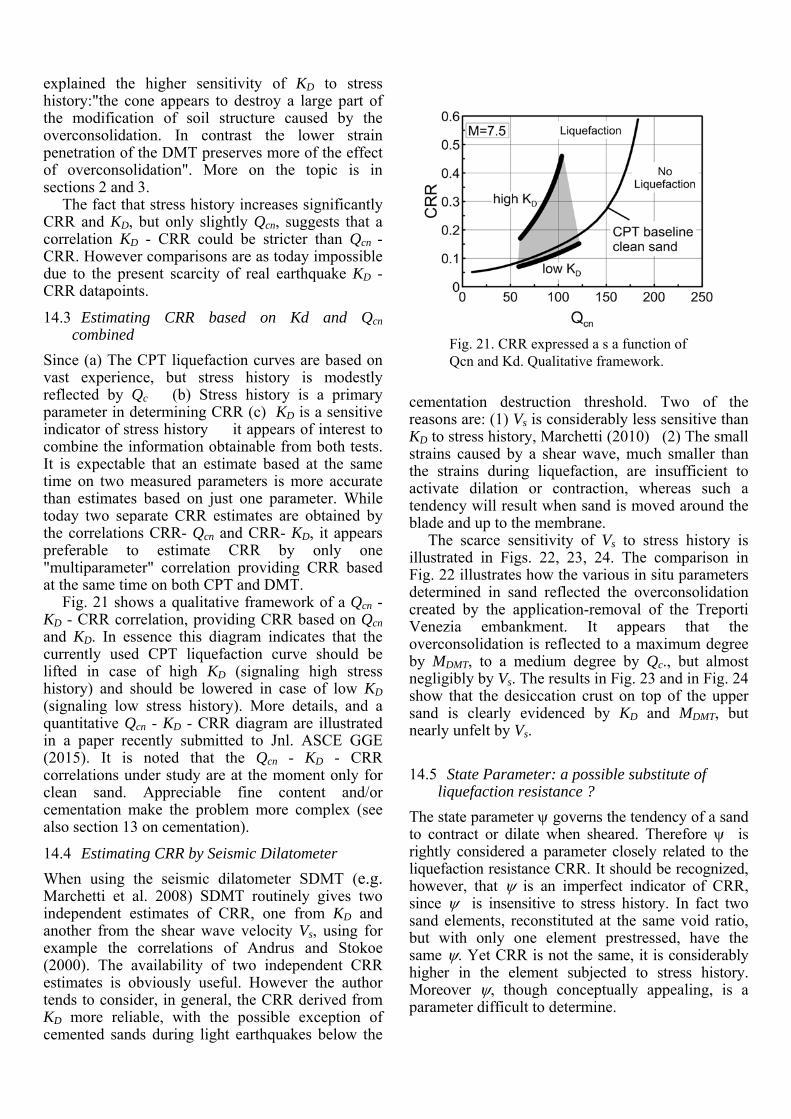
14.3 Estimating CRR based on Kd and Qcn combined

Since (a) The CPT liquefaction curves are based on vast experience, but stress history is modestly reflected by Qc (b) Stress history is a primary parameter in determining CRR (c) KD is a sensitive indicator of stress history it appears of interest to combine the information obtainable from both tests. It is expectable that an estimate based at the same time on two measured parameters is more accurate than estimates based on just one parameter. While today two separate CRR estimates are obtained by the correlations CRR- Qcn and CRR- KD, it appears preferable to estimate CRR by only one "multiparameter" correlation providing CRR based at the same time on both CPT and DMT.

Fig. 21 shows a qualitative framework of a Qcn - KD - CRR correlation, providing CRR based on Qcn and KD. In essence this diagram indicates that the currently used CPT liquefaction curve should be lifted in case of high KD (signaling high stress history) and should be lowered in case of low KD (signaling low stress history). More details, and a quantitative Qcn - KD - CRR diagram are illustrated in a paper recently submitted to Jnl. ASCE GGE (2015). It is noted that the Qcn - KD - CRR correlations under study are at the moment only for clean sand. Appreciable fine content and/or cementation make the problem more complex (see also section 13 on cementation).

14.4 Estimating CRR by Seismic Dilatometer

When using the seismic dilatometer SDMT (e.g. Marchetti et al. 2008) SDMT routinely gives two independent estimates of CRR, one from KD and another from the shear wave velocity Vs, using for example the correlations of Andrus and Stokoe (2000). The availability of two independent CRR estimates is obviously useful. However the author tends to consider, in general, the CRR derived from KD more reliable, with the possible exception of cemented sands during light earthquakes below the

cementation destruction threshold. Two of the reasons are: (1) Vs is considerably less sensitive than KD to stress history, Marchetti (2010) (2) The small strains caused by a shear wave, much smaller than the strains during liquefaction, are insufficient to activate dilation or contraction, whereas such a tendency will result when sand is moved around the blade and up to the membrane.

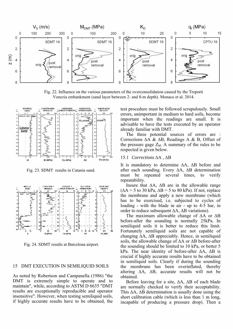
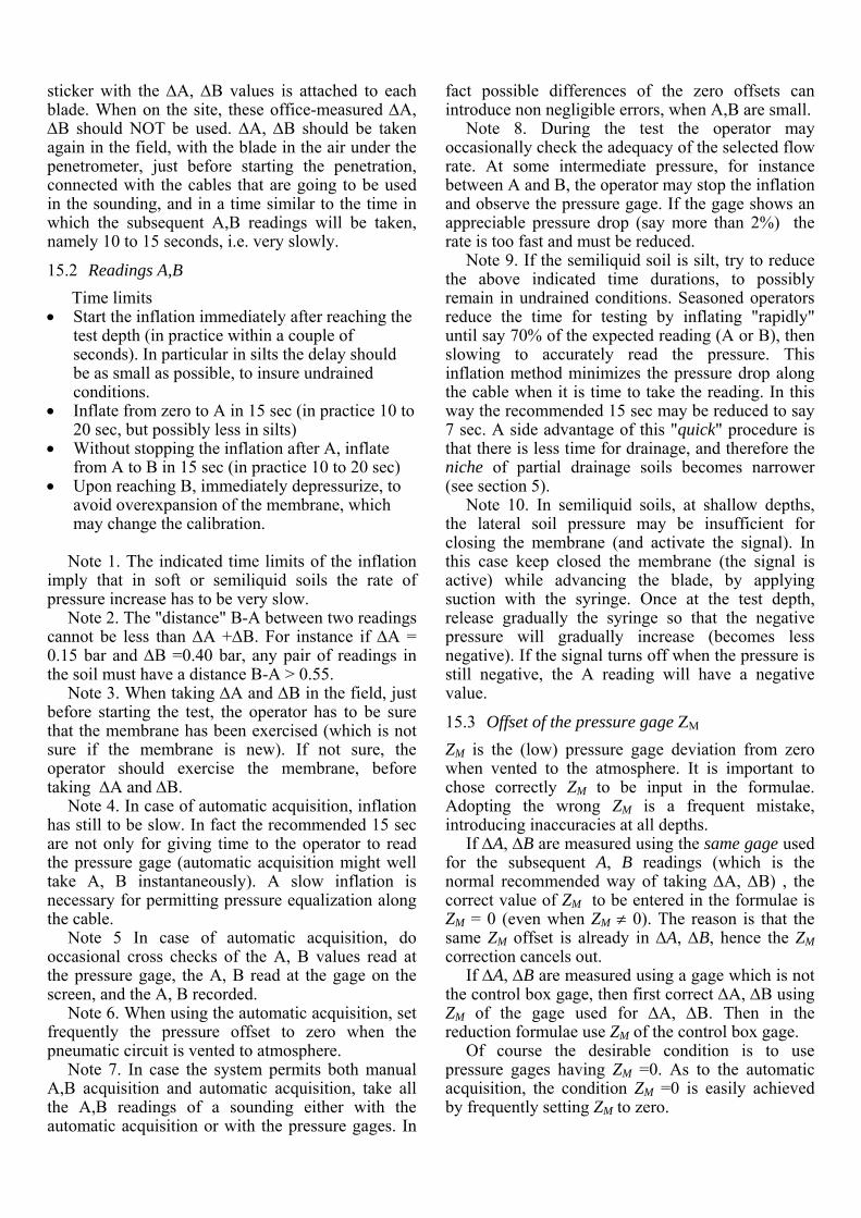
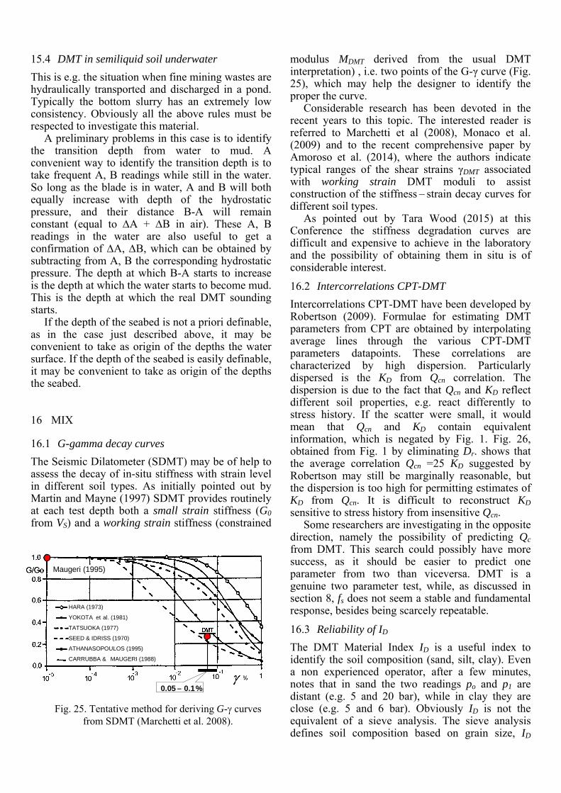
The scarce sensitivity of Vs to stress history is illustrated in Figs. 22, 23, 24. The comparison in Fig. 22 illustrates how the various in situ parameters determined in sand reflected the overconsolidation created by the application-removal of the Treporti Venezia embankment. It appears that the overconsolidation is reflected to a maximum degree by MDMT, to a medium degree by Qc., but almost negligibly by Vs. The results in Fig. 23 and in Fig. 24 show that the desiccation crust on top of the upper sand is clearly evidenced by KD and MDMT, but nearly unfelt by Vs.

14.5 State Parameter: a possible substitute of liquefaction resistance ?

The state parameter governs the tendency of a sand to contract or dilate when sheared. Therefore is rightly considered a parameter closely related to the liquefaction resistance CRR. It should be recognized, however, that is an imperfect indicator of CRR, since is insensitive to stress history. In fact two sand elements, reconstituted at the same void ratio, but with only one element prestressed, have the same . Yet CRR is not the same, it is considerably higher in the element subjected to stress history. Moreover , though conceptually appealing, is a parameter difficult to determine.

Fig. 21. CRR expressed a s a function of Qcn and Kd. Qualitative framework.

15 DMT EXECUTION IN SEMILIQUID SOILS

As noted by Robertson and Campanella (1986) "the DMT is extremely simple to operate and to maintain", while, according to ASTM D 6635 "DMT results are exceptionally reproducible and operator insensitive". However, when testing semiliquid soils, if highly accurate results have to be obtained, the

test procedure must be followed scrupulously. Small errors, unimportant in medium to hard soils, become important when the readings are small. It is advisable to have the tests executed by an operator already familiar with DMT.

The three potential sources of errors are : Corrections A & B, Readings A & B, Offset of the pressure gage ZM. A summary of the rules to be respected is given below.

15.1 Corrections A , B

It is mandatory to determine A, B before and after each sounding. Every A, B determination must be repeated several times, to verify repeatability.

Insure that A, B are in the allowable range (A = 5 to 30 kPa, B = 5 to 80 kPa). If not, replace the membrane and apply a new membrane (which has to be exercised, i.e. subjected to cycles of loading - with the blade in air - up to 4-5 bar, in order to reduce subsequent A, B variations).

The maximum allowable change of A or B before-after the sounding is normally 25kPa. In semiliquid soils it is better to reduce this limit. Fortunately semiliquid soils are not capable of changing A, B appreciably. Hence, in semiliquid soils, the allowable change of A or B before-after the sounding should be limited to 10 kPa, or better 5 kPa. The near identity of before-after A, B is crucial if highly accurate results have to be obtained in semiliquid soils. Clearly if during the sounding the membrane has been overinflated, thereby altering A, B, accurate results will not be obtained.

Before leaving for a site, A, B of each blade are normally checked to verify their acceptability. This A, B determination is usually done using the short calibration cable (which is less than 1 m long, incapable of producing a pressure drop). Then a

Fig. 23. SDMT results in Catania sand.

Fig. 22. Influence on the various parameters of the overconsolidation caused by the Treporti Venezia embankment (sand layer between 2- and 8-m depth). Monaco et al. 2014.

Fig. 24. SDMT results at Barcelona airport.

sticker with the A, B values is attached to each blade. When on the site, these office-measured A, B should NOT be used. A, B should be taken again in the field, with the blade in the air under the penetrometer, just before starting the penetration, connected with the cables that are going to be used in the sounding, and in a time similar to the time in which the subsequent A,B readings will be taken, namely 10 to 15 seconds, i.e. very slowly.

15.2 Readings A,B

Time limits Start the inflation immediately after reaching the

test depth (in practice within a couple of seconds). In particular in silts the delay should be as small as possible, to insure undrained conditions.

Inflate from zero to A in 15 sec (in practice 10 to 20 sec, but possibly less in silts)

Without stopping the inflation after A, inflate from A to B in 15 sec (in practice 10 to 20 sec)

Upon reaching B, immediately depressurize, to avoid overexpansion of the membrane, which may change the calibration.

Note 1. The indicated time limits of the inflation

imply that in soft or semiliquid soils the rate of pressure increase has to be very slow.

Note 2. The "distance" B-A between two readings cannot be less than A +B. For instance if A = 0.15 bar and B =0.40 bar, any pair of readings in the soil must have a distance B-A > 0.55.

Note 3. When taking A and B in the field, just before starting the test, the operator has to be sure that the membrane has been exercised (which is not sure if the membrane is new). If not sure, the operator should exercise the membrane, before taking A and B.

Note 4. In case of automatic acquisition, inflation has still to be slow. In fact the recommended 15 sec are not only for giving time to the operator to read the pressure gage (automatic acquisition might well take A, B instantaneously). A slow inflation is necessary for permitting pressure equalization along the cable.

Note 5 In case of automatic acquisition, do occasional cross checks of the A, B values read at the pressure gage, the A, B read at the gage on the screen, and the A, B recorded.

Note 6. When using the automatic acquisition, set frequently the pressure offset to zero when the pneumatic circuit is vented to atmosphere.

Note 7. In case the system permits both manual A,B acquisition and automatic acquisition, take all the A,B readings of a sounding either with the automatic acquisition or with the pressure gages. In

fact possible differences of the zero offsets can introduce non negligible errors, when A,B are small.

Note 8. During the test the operator may occasionally check the adequacy of the selected flow rate. At some intermediate pressure, for instance between A and B, the operator may stop the inflation and observe the pressure gage. If the gage shows an appreciable pressure drop (say more than 2%) the rate is too fast and must be reduced.

Note 9. If the semiliquid soil is silt, try to reduce the above indicated time durations, to possibly remain in undrained conditions. Seasoned operators reduce the time for testing by inflating "rapidly" until say 70% of the expected reading (A or B), then slowing to accurately read the pressure. This inflation method minimizes the pressure drop along the cable when it is time to take the reading. In this way the recommended 15 sec may be reduced to say 7 sec. A side advantage of this "quick" procedure is that there is less time for drainage, and therefore the niche of partial drainage soils becomes narrower (see section 5).

Note 10. In semiliquid soils, at shallow depths, the lateral soil pressure may be insufficient for closing the membrane (and activate the signal). In this case keep closed the membrane (the signal is active) while advancing the blade, by applying suction with the syringe. Once at the test depth, release gradually the syringe so that the negative pressure will gradually increase (becomes less negative). If the signal turns off when the pressure is still negative, the A reading will have a negative value.

15.3 Offset of the pressure gage ZM

ZM is the (low) pressure gage deviation from zero when vented to the atmosphere. It is important to chose correctly ZM to be input in the formulae. Adopting the wrong ZM is a frequent mistake, introducing inaccuracies at all depths.

If A, B are measured using the same gage used for the subsequent A, B readings (which is the normal recommended way of taking A, B) , the correct value of ZM to be entered in the formulae is ZM = 0 (even when ZM 0). The reason is that the same ZM offset is already in A, B, hence the ZM correction cancels out.

If A, B are measured using a gage which is not the control box gage, then first correct A, B using ZM of the gage used for A, B. Then in the reduction formulae use ZM of the control box gage.

Of course the desirable condition is to use pressure gages having ZM =0. As to the automatic acquisition, the condition ZM =0 is easily achieved by frequently setting ZM to zero.

15.4 DMT in semiliquid soil underwater

This is e.g. the situation when fine mining wastes are hydraulically transported and discharged in a pond. Typically the bottom slurry has an extremely low consistency. Obviously all the above rules must be respected to investigate this material.

A preliminary problems in this case is to identify the transition depth from water to mud. A convenient way to identify the transition depth is to take frequent A, B readings while still in the water. So long as the blade is in water, A and B will both equally increase with depth of the hydrostatic pressure, and their distance B-A will remain constant (equal to A + B in air). These A, B readings in the water are also useful to get a confirmation of A, B, which can be obtained by subtracting from A, B the corresponding hydrostatic pressure. The depth at which B-A starts to increase is the depth at which the water starts to become mud. This is the depth at which the real DMT sounding starts.

If the depth of the seabed is not a priori definable, as in the case just described above, it may be convenient to take as origin of the depths the water surface. If the depth of the seabed is easily definable, it may be convenient to take as origin of the depths the seabed.

16 MIX

16.1 G-gamma decay curves

The Seismic Dilatometer (SDMT) may be of help to assess the decay of in-situ stiffness with strain level in different soil types. As initially pointed out by Martin and Mayne (1997) SDMT provides routinely at each test depth both a small strain stiffness (G0 from VS) and a working strain stiffness (constrained

modulus MDMT derived from the usual DMT interpretation) , i.e. two points of the G-γ curve (Fig. 25), which may help the designer to identify the proper the curve.

Considerable research has been devoted in the recent years to this topic. The interested reader is referred to Marchetti et al (2008), Monaco et al. (2009) and to the recent comprehensive paper by Amoroso et al. (2014), where the authors indicate typical ranges of the shear strains γDMT associated with working strain DMT moduli to assist construction of the stiffness – strain decay curves for different soil types.

As pointed out by Tara Wood (2015) at this Conference the stiffness degradation curves are difficult and expensive to achieve in the laboratory and the possibility of obtaining them in situ is of considerable interest.

16.2 Intercorrelations CPT-DMT

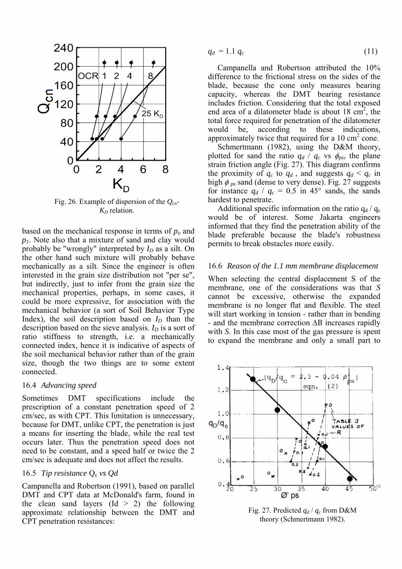
Intercorrelations CPT-DMT have been developed by Robertson (2009). Formulae for estimating DMT parameters from CPT are obtained by interpolating average lines through the various CPT-DMT parameters datapoints. These correlations are characterized by high dispersion. Particularly dispersed is the KD from Qcn correlation. The dispersion is due to the fact that Qcn and KD reflect different soil properties, e.g. react differently to stress history. If the scatter were small, it would mean that Qcn and KD contain equivalent information, which is negated by Fig. 1. Fig. 26, obtained from Fig. 1 by eliminating Dr. shows that the average correlation Qcn =25 KD suggested by Robertson may still be marginally reasonable, but the dispersion is too high for permitting estimates of KD from Qcn. It is difficult to reconstruct KD sensitive to stress history from insensitive Qcn.

Some researchers are investigating in the opposite direction, namely the possibility of predicting Qc from DMT. This search could possibly have more success, as it should be easier to predict one parameter from two than viceversa. DMT is a genuine two parameter test, while, as discussed in section 8, fs does not seem a stable and fundamental response, besides being scarcely repeatable.

16.3 Reliability of ID

The DMT Material Index ID is a useful index to identify the soil composition (sand, silt, clay). Even a non experienced operator, after a few minutes, notes that in sand the two readings po and p1 are distant (e.g. 5 and 20 bar), while in clay they are close (e.g. 5 and 6 bar). Obviously ID is not the equivalent of a sieve analysis. The sieve analysis defines soil composition based on grain size, ID

HARA (1973) YOKOTA et al. (1981) TATSUOKA (1977) SEED & IDRISS (1970) ATHANASOPOULOS (1995) CARRUBBA & MAUGERI (1988)

0.05 to 0.1%

HARA (1973) YOKOTA et al. (1981) TATSUOKA (1977) SEED & IDRISS (1970) ATHANASOPOULOS (1995) CARRUBBA & MAUGERI (1988)

0.05 – 0.1 %

Maugeri (1995)

Fig. 25. Tentative method for deriving G- curves from SDMT (Marchetti et al. 2008).

based on the mechanical response in terms of po and p1. Note also that a mixture of sand and clay would probably be "wrongly" interpreted by ID as a silt. On the other hand such mixture will probably behave mechanically as a silt. Since the engineer is often interested in the grain size distribution not "per se", but indirectly, just to infer from the grain size the mechanical properties, perhaps, in some cases, it could be more expressive, for association with the mechanical behavior (a sort of Soil Behavior Type Index), the soil description based on ID than the description based on the sieve analysis. ID is a sort of ratio stiffness to strength, i.e. a mechanically connected index, hence it is indicative of aspects of the soil mechanical behavior rather than of the grain size, though the two things are to some extent connected.

16.4 Advancing speed

Sometimes DMT specifications include the prescription of a constant penetration speed of 2 cm/sec, as with CPT. This limitation is unnecessary, because for DMT, unlike CPT, the penetration is just a means for inserting the blade, while the real test occurs later. Thus the penetration speed does not need to be constant, and a speed half or twice the 2 cm/sec is adequate and does not affect the results.

16.5 Tip resistance Qc vs Qd

Campanella and Robertson (1991), based on parallel DMT and CPT data at McDonald's farm, found in the clean sand layers (Id > 2) the following approximate relationship between the DMT and CPT penetration resistances:

qd = 1.1 qc (11)

Campanella and Robertson attributed the 10% difference to the frictional stress on the sides of the blade, because the cone only measures bearing capacity, whereas the DMT bearing resistance includes friction. Considering that the total exposed end area of a dilatometer blade is about 18 cm2, the total force required for penetration of the dilatometer would be, according to these indications, approximately twice that required for a 10 cm2 cone.

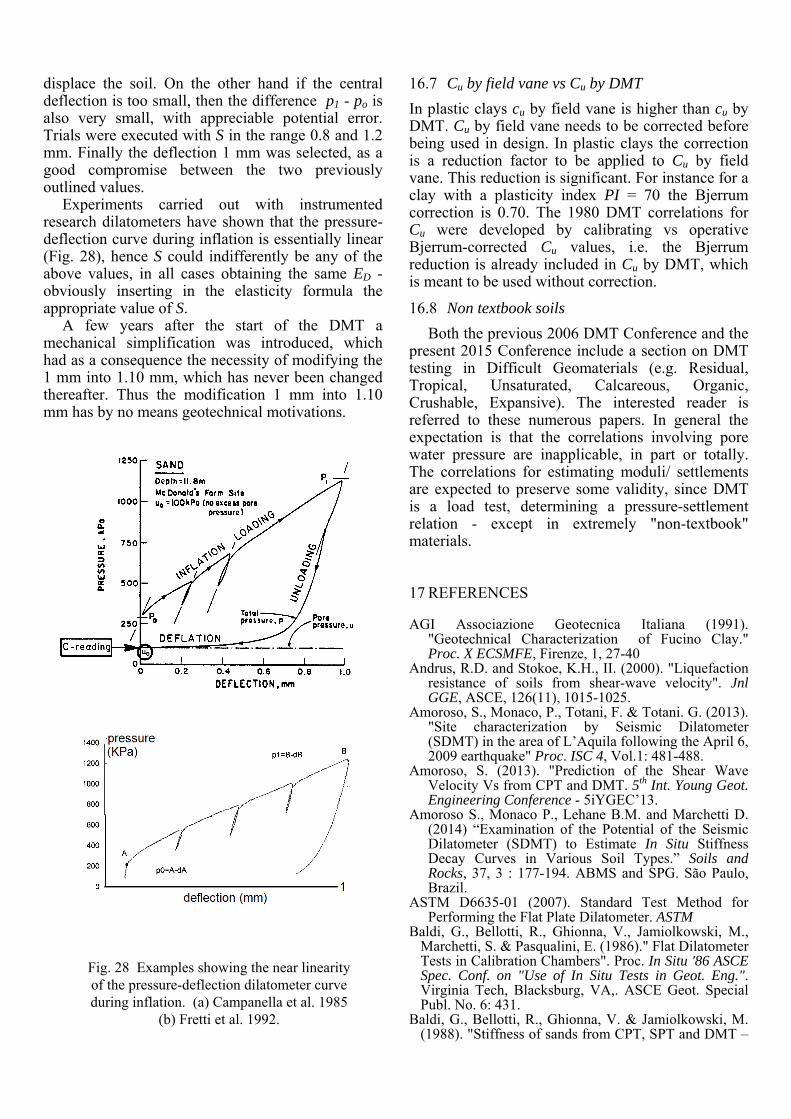
Schmertmann (1982), using the D&M theory, plotted for sand the ratio qd / qc vs ps, the plane strain friction angle (Fig. 27). This diagram confirms the proximity of qc to qd , and suggests qd < qc in high ps sand (dense to very dense). Fig. 27 suggests for instance qd / qc = 0.5 in 45° sands, the sands hardest to penetrate.

Additional specific information on the ratio qd / qc would be of interest. Some Jakarta engineers informed that they find the penetration ability of the blade preferable because the blade's robustness permits to break obstacles more easily.

16.6 Reason of the 1.1 mm membrane displacement

When selecting the central displacement S of the membrane, one of the considerations was that S cannot be excessive, otherwise the expanded membrane is no longer flat and flexible. The steel will start working in tension - rather than in bending - and the membrane correction B increases rapidly with S. In this case most of the gas pressure is spent to expand the membrane and only a small part to

Fig. 27. Predicted qd / qc from D&M theory (Schmertmann 1982).

Fig. 26. Example of dispersion of the Qcn-KD relation.

displace the soil. On the other hand if the central deflection is too small, then the difference p1 - po is also very small, with appreciable potential error. Trials were executed with S in the range 0.8 and 1.2 mm. Finally the deflection 1 mm was selected, as a good compromise between the two previously outlined values.

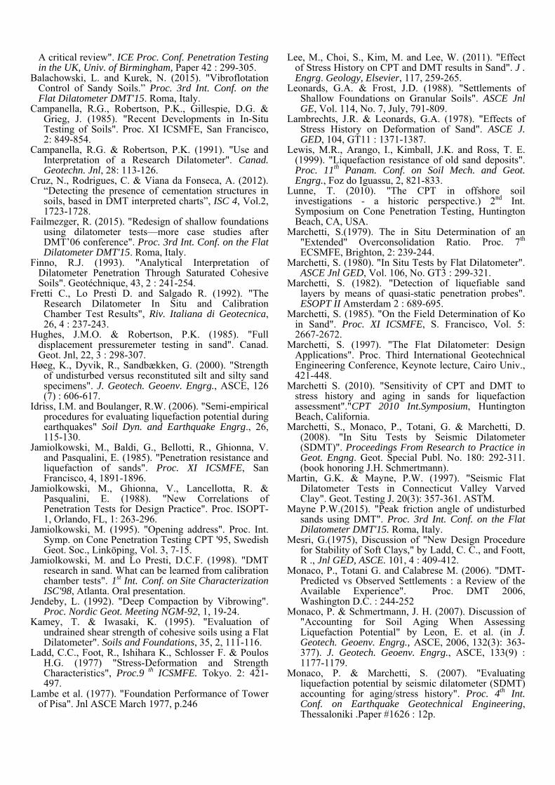
Experiments carried out with instrumented research dilatometers have shown that the pressure-deflection curve during inflation is essentially linear (Fig. 28), hence S could indifferently be any of the above values, in all cases obtaining the same ED - obviously inserting in the elasticity formula the appropriate value of S.

A few years after the start of the DMT a mechanical simplification was introduced, which had as a consequence the necessity of modifying the 1 mm into 1.10 mm, which has never been changed thereafter. Thus the modification 1 mm into 1.10 mm has by no means geotechnical motivations.

16.7 Cu by field vane vs Cu by DMT

In plastic clays cu by field vane is higher than cu by DMT. Cu by field vane needs to be corrected before being used in design. In plastic clays the correction is a reduction factor to be applied to Cu by field vane. This reduction is significant. For instance for a clay with a plasticity index PI = 70 the Bjerrum correction is 0.70. The 1980 DMT correlations for Cu were developed by calibrating vs operative Bjerrum-corrected Cu values, i.e. the Bjerrum reduction is already included in Cu by DMT, which is meant to be used without correction.

16.8 Non textbook soils

Both the previous 2006 DMT Conference and the present 2015 Conference include a section on DMT testing in Difficult Geomaterials (e.g. Residual, Tropical, Unsaturated, Calcareous, Organic, Crushable, Expansive). The interested reader is referred to these numerous papers. In general the expectation is that the correlations involving pore water pressure are inapplicable, in part or totally. The correlations for estimating moduli/ settlements are expected to preserve some validity, since DMT is a load test, determining a pressure-settlement relation - except in extremely "non-textbook" materials.

17 REFERENCES

AGI Associazione Geotecnica Italiana (1991). "Geotechnical Characterization of Fucino Clay." Proc. X ECSMFE, Firenze, 1, 27-40

Andrus, R.D. and Stokoe, K.H., II. (2000). "Liquefaction resistance of soils from shear-wave velocity". Jnl GGE, ASCE, 126(11), 1015-1025.

Amoroso, S., Monaco, P., Totani, F. & Totani. G. (2013). "Site characterization by Seismic Dilatometer (SDMT) in the area of L’Aquila following the April 6, 2009 earthquake" Proc. ISC 4, Vol.1: 481-488.

Amoroso, S. (2013). "Prediction of the Shear Wave Velocity Vs from CPT and DMT. 5th Int. Young Geot. Engineering Conference - 5iYGEC’13.

Amoroso S., Monaco P., Lehane B.M. and Marchetti D. (2014) “Examination of the Potential of the Seismic Dilatometer (SDMT) to Estimate In Situ Stiffness Decay Curves in Various Soil Types.” Soils and Rocks, 37, 3 : 177-194. ABMS and SPG. São Paulo, Brazil.

ASTM D6635-01 (2007). Standard Test Method for Performing the Flat Plate Dilatometer. ASTM

Baldi, G., Bellotti, R., Ghionna, V., Jamiolkowski, M., Marchetti, S. & Pasqualini, E. (1986)." Flat Dilatometer Tests in Calibration Chambers". Proc. In Situ '86 ASCE Spec. Conf. on "Use of In Situ Tests in Geot. Eng.". Virginia Tech, Blacksburg, VA,. ASCE Geot. Special Publ. No. 6: 431.

Baldi, G., Bellotti, R., Ghionna, V. & Jamiolkowski, M. (1988). "Stiffness of sands from CPT, SPT and DMT –

Fig. 28 Examples showing the near linearity of the pressure-deflection dilatometer curve during inflation. (a) Campanella et al. 1985

(b) Fretti et al. 1992.

A critical review". ICE Proc. Conf. Penetration Testing in the UK, Univ. of Birmingham, Paper 42 : 299-305.

Balachowski, L. and Kurek, N. (2015). "Vibroflotation Control of Sandy Soils.” Proc. 3rd Int. Conf. on the Flat Dilatometer DMT'15. Roma, Italy.

Campanella, R.G., Robertson, P.K., Gillespie, D.G. & Grieg, J. (1985). "Recent Developments in In-Situ Testing of Soils". Proc. XI ICSMFE, San Francisco, 2: 849-854.

Campanella, R.G. & Robertson, P.K. (1991). "Use and Interpretation of a Research Dilatometer". Canad. Geotechn. Jnl, 28: 113-126.

Cruz, N., Rodrigues, C. & Viana da Fonseca, A. (2012). “Detecting the presence of cementation structures in soils, based in DMT interpreted charts”, ISC 4, Vol.2, 1723-1728.

Failmezger, R. (2015). "Redesign of shallow foundations using dilatometer tests—more case studies after DMT’06 conference". Proc. 3rd Int. Conf. on the Flat Dilatometer DMT'15. Roma, Italy.

Finno, R.J. (1993). "Analytical Interpretation of Dilatometer Penetration Through Saturated Cohesive Soils". Geotéchnique, 43, 2 : 241-254.

Fretti C., Lo Presti D. and Salgado R. (1992). "The Research Dilatometer In Situ and Calibration Chamber Test Results", Riv. Italiana di Geotecnica, 26, 4 : 237-243.

Hughes, J.M.O. & Robertson, P.K. (1985). "Full displacement pressuremeter testing in sand". Canad. Geot. Jnl, 22, 3 : 298-307.

Høeg, K., Dyvik, R., Sandbækken, G. (2000). "Strength of undisturbed versus reconstituted silt and silty sand specimens". J. Geotech. Geoenv. Engrg., ASCE, 126 (7) : 606-617.

Idriss, I.M. and Boulanger, R.W. (2006). "Semi-empirical procedures for evaluating liquefaction potential during earthquakes" Soil Dyn. and Earthquake Engrg., 26, 115-130.

Jamiolkowski, M., Baldi, G., Bellotti, R., Ghionna, V. and Pasqualini, E. (1985). "Penetration resistance and liquefaction of sands". Proc. XI ICSMFE, San Francisco, 4, 1891-1896.

Jamiolkowski, M., Ghionna, V., Lancellotta, R. & Pasqualini, E. (1988). "New Correlations of Penetration Tests for Design Practice". Proc. ISOPT-1, Orlando, FL, 1: 263-296.

Jamiolkowski, M. (1995). "Opening address". Proc. Int. Symp. on Cone Penetration Testing CPT '95, Swedish Geot. Soc., Linköping, Vol. 3, 7-15.

Jamiolkowski, M. and Lo Presti, D.C.F. (1998). "DMT research in sand. What can be learned from calibration chamber tests". 1st Int. Conf. on Site Characterization ISC'98, Atlanta. Oral presentation.

Jendeby, L. (1992). "Deep Compaction by Vibrowing". Proc. Nordic Geot. Meeting NGM-92, 1, 19-24.

Kamey, T. & Iwasaki, K. (1995). "Evaluation of undrained shear strength of cohesive soils using a Flat Dilatometer". Soils and Foundations, 35, 2, 111-116.

Ladd, C.C., Foot, R., Ishihara K., Schlosser F. & Poulos H.G. (1977) "Stress-Deformation and Strength Characteristics", Proc.9 th ICSMFE. Tokyo. 2: 421-497.

Lambe et al. (1977). "Foundation Performance of Tower of Pisa". Jnl ASCE March 1977, p.246

Lee, M., Choi, S., Kim, M. and Lee, W. (2011). "Effect of Stress History on CPT and DMT results in Sand". J . Engrg. Geology, Elsevier, 117, 259-265.

Leonards, G.A. & Frost, J.D. (1988). "Settlements of Shallow Foundations on Granular Soils". ASCE Jnl GE, Vol. 114, No. 7, July, 791-809.

Lambrechts, J.R. & Leonards, G.A. (1978). "Effects of Stress History on Deformation of Sand". ASCE J. GED, 104, GT11 : 1371-1387.

Lewis, M.R., Arango, I., Kimball, J.K. and Ross, T. E. (1999). "Liquefaction resistance of old sand deposits". Proc. 11th Panam. Conf. on Soil Mech. and Geot. Engrg., Foz do Iguassu, 2, 821-833.

Lunne, T. (2010). "The CPT in offshore soil investigations - a historic perspective.) 2nd Int. Symposium on Cone Penetration Testing, Huntington Beach, CA, USA.

Marchetti, S.(1979). The in Situ Determination of an "Extended" Overconsolidation Ratio. Proc. 7th ECSMFE, Brighton, 2: 239-244.

Marchetti, S. (1980). "In Situ Tests by Flat Dilatometer". ASCE Jnl GED, Vol. 106, No. GT3 : 299-321.

Marchetti, S. (1982). "Detection of liquefiable sand layers by means of quasi-static penetration probes". ESOPT II Amsterdam 2 : 689-695.

Marchetti, S. (1985). "On the Field Determination of Ko in Sand". Proc. XI ICSMFE, S. Francisco, Vol. 5: 2667-2672.

Marchetti, S. (1997). "The Flat Dilatometer: Design Applications". Proc. Third International Geotechnical Engineering Conference, Keynote lecture, Cairo Univ., 421-448.

Marchetti S. (2010). "Sensitivity of CPT and DMT to stress history and aging in sands for liquefaction assessment"."CPT 2010 Int.Symposium, Huntington Beach, California.

Marchetti, S., Monaco, P., Totani, G. & Marchetti, D. (2008). "In Situ Tests by Seismic Dilatometer (SDMT)". Proceedings From Research to Practice in Geot. Engng. Geot. Special Publ. No. 180: 292-311. (book honoring J.H. Schmertmann).

Martin, G.K. & Mayne, P.W. (1997). "Seismic Flat Dilatometer Tests in Connecticut Valley Varved Clay". Geot. Testing J. 20(3): 357-361. ASTM.

Mayne P.W.(2015). "Peak friction angle of undisturbed sands using DMT". Proc. 3rd Int. Conf. on the Flat Dilatometer DMT'15. Roma, Italy.

Mesri, G.(1975), Discussion of "New Design Procedure for Stability of Soft Clays," by Ladd, C. C., and Foott, R ., Jnl GED, ASCE. 101, 4 : 409-412.

Monaco, P., Totani G. and Calabrese M. (2006). "DMT- Predicted vs Observed Settlements : a Review of the Available Experience". Proc. DMT 2006, Washington D.C. : 244-252

Monaco, P. & Schmertmann, J. H. (2007). Discussion of "Accounting for Soil Aging When Assessing Liquefaction Potential" by Leon, E. et al. (in J. Geotech. Geoenv. Engrg., ASCE, 2006, 132(3): 363-377). J. Geotech. Geoenv. Engrg., ASCE, 133(9) : 1177-1179.

Monaco, P. & Marchetti, S. (2007). "Evaluating liquefaction potential by seismic dilatometer (SDMT) accounting for aging/stress history". Proc. 4th Int. Conf. on Earthquake Geotechnical Engineering, Thessaloniki .Paper #1626 : 12p.

Monaco, P., Marchetti, S., Totani, G. and Marchetti,D. (2009 "Interrelationship between small strain modulus G0 and operative modulus" Proc. IS-Tokyo 2009, Tsukuba, 1315-1323.

Monaco et al. (2014). "Overconsolidation and stiffness of Venice Lagoon Sands and Silts from SDMT and CPTU". Jnl Asce GGE. Jan 2014 : 215-227

Pyke, R. (2003). Discussion of "Liquefaction Resistance of Soils: Summary Report from the 1996 NCEER and 1998 NCEER/NSF". Jnl GGE, ASCE, 129(3), 283-284.

Robertson, P.K. (2009). "CPT-DMT Correlations". ASCE J. GGE, 135.11, 1762-1771.

Robertson, P.K. (2012). "Mitchell Lecture. Interpretation of in-situ tests - some insight." Proc. ISC-4, Porto de Galinhas - Brazil, 1, 3-24.

Robertson, P.K. and Campanella, R.G. (1983). "Interpretation of Cone Penetration Test". Canad. G. Jnl, 20, p. 722.

Robertson, P.K., Campanella, R.G., Gillespie, D. and Rice, A. (1986). "Seismic CPT to measure in-situ shear Wave Velocity" ASCE J. GED, 112, 8, 791-803.

Robertson, P.K. & Campanella, R.G. (1986). "Estimating Liquefaction Potential of Sands Using the Flat Plate Dilatometer". ASTM Geotechn. Testing Journal, 9(1) : 38-40.

Rocha, B.P., Castro. B.A.C.and Giacheti H.L. (2015). "Seismic DMT Test in a Non-Text Book Type Geomaterial" Proc. 3rd Int. Conf. on the Flat Dilatometer DMT'15. Roma, Italy.

Salgado, R., Boulanger,R.W. and Mitchell, J.K. (1997). "Lateral Stress Effects on CPT Liquefaction Resistance Correlations". ASCE J. GGE, 123.08, 726-735.

Sharif, E. (2015). "Early Applications of DMT in Dubai in Two Main Projects for Natural Sharif Artificial Earthfill Silty Sand". Proc. 3rd Int. Conf. on the Flat Dilatometer DMT'15. Roma, Italy.

Schmertmann, J.H. (1982). "A Method for Determining the Friction Angle in Sands from the Marchetti Dilatometer Test (DMT)". Proc. 2nd European Symp. on Penetration Testing, Amsterdam. 2: 853.

Schmertmann, J.H. (1983). "Revised Procedure for Calculating Ko and OCR from DMT's with Id>1.2 and which Incorporates the Penetration Measurement to Permit Calculating the Plane Strain Friction Angle". DMT Digest No. 1. GPE Inc., Gainesville, Florida, U.S.A.

Schmertmann, J.H. (1984). "Comparing DMT with CPT in NC/OC Sand Bucket test." Digest No. 4 Section 4D. GPE Inc., Gainesville, Florida, U.S.A.

Schmertmann, J.H. (1986). "Dilatometer to compute Foundation Settlement". Proc. In Situ '86, ASCE Spec. Conf. on "Use of In Situ Tests in Geotechn. Engineering", Virginia Tech, Blacksburg, VA, ASCE Geot. Special Publ. No. 6, 303-321.

Schmertmann, J.H. (1988). "Dilatometers Settle In", Civil Engineering ASCE , March 1988

Schmertmann, J.H., Baker, W., Gupta, R. & Kessler, K. (1986). "CPT/DMT Quality Control of Ground Modification at a Power Plant". Proc. In Situ '86 ASCE Spec. Conf. VIP, Blacksburg, Geot. Spec. Publ. No. 6, 985-1001.

Schnaid F. "2009"."In Situ Testing in Geomechanics – the main tests". Taylor and Francis Group, London: Book 327 p.

Schnaid, F., Lehane, B. & Fahey, M. 2004. "In-situ test characterization of unusual geomaterial". Proc. ISC’2, Porto, 2004. 1, 49-73

TC16 DMT Report (2001). “The Flat Dilatometer Test (DMT) in Soil Investigations”. A Report by the ISSMGE Committee TC16. 41 pp. Reprinted in Proc. DMT 2006, Washington D.C.

Wood, T. (2015). "Re-appraisal of the Dilatometer for In-situ Assessment of Geotechnical Properties of Swedish glacio-marine clays". Proc. 3rd Int. Conf. on the Flat Dilatometer DMT'15. Roma, Italy.

Youd, T.L. and Idriss, I.M. (2001). "Liquefaction Resistance of Soils: Summary Report from the 1996 NCEER and 1998 NCEER/NSF Workshops on Evaluation of Liquefaction Resistance of Soils". Jnl GGE, ASCE, 127(4), 297-313.

Yoshimi,Y, Kuwabara, F.and Tokimatsu. K. (1975). "One-dimensional Volume Change characteristics of sands under very low confining stresses". Soils and Foundations, 15, 51-60.

Yu, H.S. 2004. "In situ soil testing: from mechanics to interpretation". 1st J.K. Mitchell Lecture, Proc. ISC-2, Porto. 1: 3-38.