Magnetismo basico

2 BASIC MAGNETISM

2.1 DIAMAGNETISM, PARAMAGNETISM, FERROMAGNETISM

The classical theories of both diamagnetism and paramagnetism first appeared in 1905 in a paper by Paul Langevin (1872-1946). Diamagnetism is a property of all materials. It arises from the interaction of an applied magnetic field and the motion of electrons orbiting the nucleus. Because electrons carry charge, they experience a sideways Lorentz force (Hendrik Lorentz, 1853-1928) when moving through a magnetic field. The outcome can be appreciated from a simple case involving an electron traveling clockwise in a circular orbit centered at the origin and lying in the xy plane, with an external magnetic field applied in the +x direction. For half the orbit (x > 0), the Lorentz force will parallel -z ; for the other half, it will parallel +z. A torque therefore arises parallel to the y axis, and this causes the orbit to precess-- like a gyroscope--around the field direction. This so-called Larmor precession (Joseph Larmor, 1857-1942) gives rise to a magnetic moment in the opposite direction to the applied field. For our purpose, the effect is so small that it can almost always be neglected. It is typically a hundred times smaller than paramagnetism and a hundred thousand times smaller than ferromagnetism. Quartz (SiO2) and many other minerals that occur naturally in sediments, rocks, and soils are diamagnetic, as is water. There are certain cases, then, where the diamagnetic signal from these substances may become appreciable. One example is the weakly magnetized water- saturated sediment sometimes encountered in lake studies. Another occurs in the laboratory when samples are heated for various experiments. For this purpose, quartz sample holders are often used. Now diamagnetism is independent of temperature, whereas paramagnetism and ferromagnetism decrease markedly as the sample is heated. At high temperatures, therefore, the diamagnetism of the sample holder itself may complicate the experimental results.

In the context of environmental magnetism, paramagnetism is much more important than diamagnetism. It arises by virtue of the fact that the electron behaves as though it were spinning about its own axis as well as orbiting the nucleus. It therefore possesses a spin magnetic moment in addition to its orbital magnetic moment. The

8 2 Basic Magnetism

total magnetic moment of an atom is given by the vector sum of all the electronic moments. If the spin and orbital magnetic moments of an atom are oriented in such a way as to cancel one another out, the atom has zero magnetic moment. This leads to diamagnetic behavior. If, on the other hand, the cancellation is only partial, the atom has a permanent magnetic moment. This leads to paramagnetism. For example, sodium has one unpaired electron in its 3s subshell. Such atoms will tend to be aligned by an external magnetic field, but thermal energy will always prevent perfect alignment. Consequently, the resulting magnetization decreases as temperature increases, the balance being a matter of statistics. Many minerals of interest to environmental studies are paramagnetic, although they generally turn out to produce "noise" rather than "signal." Nevertheless, it is important to monitor possible paramagnetic contributions to the net magnetization of a sample in order to isolate properly the ferromagnetic component, which is usually where environmental information is encoded.

Ferromagnetism is much stronger than diamagnetism and paramagnetism. It is particularly associated with the elements iron (hence the name), nickel, and cobalt but also occurs in many natural minerals such as certain very important iron oxides described in Chapter 3. Because of its unfilled 3d subshell, the iron atom possesses a fundamental magnetic moment of 4 Bohr magnetons (4/~ B, see Box 2.1) (Niels Bohr, 1885-1962). In the crystal lattice of ferromagnetic materials, adjacent atoms are sufficiently close together that some of the electron orbitals overlap and a strong interaction arises. This so-called exchange coupling means that, rather than being directed at random, the magnetic moments of all the atoms in the lattice are aligned,

Box 2.1 Bohr Magneton

All electrons behave like microscopic magnets with a fundamental quantity of magnetic moment called the Bohr magneton, #B. Its magnitude is given by eh/4~rm, e and m being the electron charge and mass and h being Planck's constant; substituting the appropriate values for these fundamental quantities leads to #B = 9.27 • 10 -24 Am 2. Each electron subshell in an atom can accept a maximum number of electrons arranged with their magnetic moments aligned in either of two antiparallel directions. A filled subshell has an even number of electrons and therefore has zero magnetic moment. We are particularly interested in the element iron. Its 26 electrons are arranged like this: ls22s22p63s23p63d64s 2. All the subshells are full except for 3d, which is four electrons short of the full d-subshell complement. The six electrons in the 3d subshell provide a net magnetic moment of 4#B because they are aligned five in one direction and only one in the opposite direction, following a basic requirement of quantum mechanics known as Hund's rule.

ls 2s 2p 3s 3p 3d 4s

2.2 Magnetic Susceptibility 9

giving rise to a strong magnetization. This arrangement is usually depicted as a regular array of arrows, all the same length and all parallel. This is ferromagnetism in its simplest form, but exchange coupling can give rise to other configurations.

In antiferromagnetism, the atomic magnets all have the same strength but neigh- boring atoms have oppositely directed moments. Although possessing strong exchange coupling, such materials have zero net magnetization. In some cases, however, a weak magnetization can arise from lattice defects and vacancies or from situations in which the atomic moments are slightly tilted out of perfect antiparallel- ism (spin canting).

There is yet another important way in which exchange coupling acts, giving rise to the phenomenon of ferrimagnetism. Here, the crystal lattice contains two kinds of sites with cations in two different coordination states. The outcome, in terms of our mental picture, is that two types of arrow are required, one longer than the other. As in antiferromagnetism, the two sets are opposed, but a strong magnetization can obviously arise if the two types are sufficiently unequal. This point will be discussed further in Chapter 3 in the context of specific minerals of interest.

2.2 M A G N E T I C SUSCEPTIBILITY

Suppose a suitable piece of a material in which we are interested is placed in a uniform magnetic field (H) and thereby acquires a magnetization per unit volume of M (Fig. 2.1). Its magnetic susceptibility (K) is defined as the magnetization acquired per unit field,

K - M / H (2.1)

In SI units, both M and H are measured in A/m, so K is dimensionless. Strictly speaking, K is called the volume susceptibility: to obtain what is called the mass susceptibility, we divide by the density (p),

• = K/p (2.2)

Because K is dimensionless, X has units of reciprocal density, m 3/kg. In some situations, it is more convenient to introduce the magnetic moment of the

entire body. This is simply given by the product Mv, where v is the total volume, the resulting units being Am 2.

In diamagnetic materials, the precessing electrons give rise to values of X on the order of 10 -8 m3/kg. Water is one of the strongest, with • -0.90 • 10 -8 m3/kg, many common rock-forming silicates, such as quartz and calcite, having values about half as large.

Paramagnetic materials have strongly temperature-dependent susceptibilities described by Curie's law (Pierre Curie, 1859-1906),

K = C / T (2.3)

10 2 Basic Magnetism

MAGNETIC SUSCEPTIBILITY

H v

H = magnetic field [A/m]

M = magnetization/volume [A/m]

v = volume [m31

p = density [kg/m 3]

Volume susceptibility

Mass susceptibility

K: = M/H [dimensionless]

X = rJp [m3/kg]

Magnetic moment = Mv [Am 2]

Figure 2.1 Definition of magnetic susceptibility and related parameters.

where T is absolute temperature and C is Curie's constant (see Box 2.2). At room temperature, the thermal energy tending to disrupt alignment is thousands of times greater than the magnetic energy trying to align the atomic moments, m. For n atoms, the result is that the net magnetization is a small fraction of the total maximum, nm.

This can be approached only at very low temperatures or by the application of extremely high fields. At room temperature, one needs fields on the order of 109A/m, whereas a typical laboratory electromagnet can reach only about 106 A/m. This means that, for all practical purposes, if we experimentally determine a graph of M versus H for a paramagnet, it will be restricted to a region near the origin where the relationship is linear, the slope being equal to the susceptibility. The mass susceptibilities (• of common rock-forming silicates, such as fayalite or biotite and the iron sulfide pyrite, are typically about 5 x 10 .7 m 3/kg (within a factor of 2).

In ferromagnetic materials, the relationship between M and H is more compli- cated (and consequently more interesting) than those for diamagnets and paramagnets. One important difference is that it is relatively easy to achieve saturation, where all the atomic moments are aligned. In some cases, this occurs in fields that are well within the range of laboratory electromagnets. Normal practice, therefore, is to measure at low fields (less than ~ 103 A/m) near the origin of the M - H graph. The

2.2 Magnetic Susceptibility 11

Box 2.2 Curie's Law

Paramagnetism arises from the tendency of atomic magnetic moments, m, to be aligned by an external magnetic field, H, all the time opposed by the disrupting effect of thermal energy. At any given temperature, the balance of thermal and magnetic energies leads to a statistical alignment such that the probability of finding an atomic moment at an angle 0 to the magnetic field depends exponen- tially on the ratio of the two energies, that is, emH c o s O/kT (where k is Boltzmann's constant and T is absolute temperature). The weakness of the alignment can readily be checked by substituting typical values. Considering atoms with a magnetic moment of 1 Bohr magneton in typical laboratory fields at room temperature leads to m H / k T ( = ~) in the range 10 -3 to 10 -4. Thermal pertur- bations vastly outweigh magnetic alignment. The actual magnetization is given by

M - nm(coth(a)- 1/o0 - nmL(oO

where n is the total number of atoms and L(ot) is called the Langevin function. For small or, L(~) is approximately equal to or/3, and Curie's law is obtained:

K = M / H = nm2/3kT = C / T

slope then gives the low-field susceptibility (alternatively called the initial suscepti- b i l i t y - b u t note that the word "initial" is often omitted). A much more important consideration, however, is the inevitable tendency of strongly magnetic objects to demagnetize themselves (see Box 2.3). The result is that the measured susceptibility is given by

K -- Ki/(1 -+- NKi) (2.4)

where Ki is the actual intrinsic susceptibility that would be measured in the absence of a demagnetizing field. Experimentally, this can be arranged by using a ring-shaped sample, called a Rowland ring after its inventor Henry Rowland (1848-1901). The demagnetizing factor, N, is simply determined by the shape of the sample. For a sphere, it is 1/3. For such a sample, as Ki increases by an order of magnitude from 10 to 100, K changes by only 26% (from 2.31 to 2.91, in fact). In the limit, K approaches 1/N, and the measured susceptibility is completely controlled by the shape of the sample. This is clearly illustrated in Fig. 2.2: a material with an intrinsic susceptibility of 100, for example, suffers a reduction of 97% as the sample shape varies from a long rod to a sphere.

We have discussed the phenomenon of demagnetization in terms of bulk material, but the same arguments hold for typical environmental samples. Now, however, the control is exerted by the shape of the individual magnetic mineral grains inside the sample, not the overall shape of the sample itself. Of course, the grains inside


Box 2.3 Demagnetizing Factor

Consider an elongated sample situated in an external field, H, applied parallel to the sample's long axis. It becomes magnetized as shown in the inset diagram, with magnetic poles at each end. These poles produce a field inside the sample, Hd, which is opposed to H.

z v

O O

Ii

.=_ 0.1 N I1) E

t~ E I1) (:3

. . . . . . . . . . . . + i ! i i i - . . . . . . . . . . . . . . . . . . . . . . . . .

0.011 0.1 1

Axial Ratio

This demagnetizing fieM depends on the shape of the sample and its magnetization (M), that is, Hd = N M , where N is the so-called demagnetizing factor.

Thus,

ninternal - - H - Hd = H - N M = H - N(Kininternal)

where Ki is the intrinsic susceptibility of the material. The susceptibility actually observed is

K = M / H = [ K i n i n t e r n a l ] / [ n i n t e r n a l ( 1 -I- NKi)] - - Ki/(1 -I- NKi) .

If the sample is long and thin, the poles are far apart, N approaches zero, and the effect is negligible. The simplest case to deal with mathematically is the ellipsoid of revolution. For a prolate ellipsoid (wherein one axis is longer than the other two), N is only about 0.02 for an axial ratio of 10:1. However, when the sample is more equidimensional, the demagnetizing effect cannot be neglected. For example, in the case of a sphere, N = 1/3 (see the accompanying graph).

the sample will not generally be aligned, so some form of spatial averaging will take place. Specific minerals of interest will be discussed in detail in Chapter 3. For the moment, we consider the useful example of a population of roughly equidimensional grains of magnetite (Fe304): it is found experimentally that the susceptibility of most well-characterized samples falls in the range 3.1 + 0.4 SI (Heider et al., 1996), which corresponds to 5.2 • 10 -4 m3/kg < • < 6.7 • 10 -4 m3/kg. Recall that this is approximately a thousand times greater than that of most relevant paramagnetic materials and a hundred thousand times greater than most diamagnetic values.

100 , w , i , | ' | I , O 0 | ~ | ~ w ,

10

o

"0 (D

1

2~

0.1

2.3 Magnetic Hysteresis 13

I I I I I I I [ I I | | i | | i

10 100

Intrinsic susceptibility Ki

Figure 2.2 This plot shows the drastic effect of demagnetization on measured susceptibility (K) for materials of high intrinsic susceptibility (Ki). For an infinitely long rod there is no reduction, whereas for a sphere (axial ratio 1:1) susceptibility is reduced by more than a factor of 30.

2.3 M A G N E T I C H Y S T E R E S I S

In the previous section, discussion centered on magnetic susceptibility, which measures the ability of a substance to acquire magnetization while the external magnetic field (H) is being applied. This is referred to as the induced magnetization. For diamagnets and paramagnets, when the external field is removed, the magnetization disappears. But for ferromagnets, this is not so. This feature is usually investigated by first applying a strong field so that the magnetization (M) is saturated (Fig. 2.3). As H is then decreased to zero, M does not fall to the origin. This is the phenomenon of magnetic hysteresis: it leaves the sample with a permanent magnetization, or magnetic remanence. If the field is now increased in the negative direction, M gradually falls to zero and then reverses and eventually saturates again. Repeated cycling of H traces out a hysteresis loop.

It is useful to identify and name certain key points on such a loop, as indicated in Figure 2.3. After application of a sufficiently high field, the sample acquires its saturation magnetization (Ms). Removal of this field leaves the sample with its saturation remanence (Mrs), but if the original field was insufficient to achieve saturation, we speak only of the sample's remanence (Mr). Application of a reversed field to Mrs eventually leads to the point where the overall magnetization, M, equals zero. The field necessary to achieve this is called the coercive force (He). [This quantity is not really a force (which would be measured in newtons), but the picturesque old- fashioned term is still universally app l i ed - - i t has the merit of conjuring up the


Ms

M,, 11 / /

I

Hcr H

Figure 2.3 Magnetic hysteresis. Several key points are labeled on the axes and explained in the text. The initial susceptibility (K) is given by the slope of the M - I t curve in low fields. He is known as the coercive force, whereas the field necessary to reduce Mrs to zero is called the coercivity of remanence, Hcr.

picture of an unwilling sample yielding under the action of an external agent.] To arrive at the point where the sample has zero remanence after the removal of the field (i.e., to get to the origin of the M - H graph), a somewhat stronger negative field is required. This is called the coercivity of remanence (Hcr). These four key elements of the hysteresis loop (Ms, Mrs, He, and Her) turn out to be extremely useful diagnostic tools. A few typical hysteresis loops are shown in Fig. 2.4. In Chapter 4, we will see how they are applied to environmental problems. However, let us not overlook the great technological importance of hysteresis. Two remanence points (+Mr and -Mr) provide the two states necessary for a binary system (1 and 0), from which it is a short step to magnetic recording, the basis of all modern computer hard drives.

2.4 GRAIN SIZE EFFECTS

If you were to look inside a magnetized ferromagnet, you would discover that it is divided into small regions in which the magnetization is uniform but that the magnetization vector within each region differs from that of its neighbors. This is why Mrs < Ms (see Fig. 2.3). These regions are called magnetic domains (Fig. 2.5).

2.4 Grain Size Effects 15

...... 8

'7 ~ 4 ~" 0 (a)

9 - 4

~ - 8 , , ~ -o.3-o.2-o.1 o o'.1 o12 o.3

Field (T)

~ - 8 . . . . :~ -0.3-0.2-0.1 0 0.1 0.2 0.3

Field (T)

1.0 (c) 0.5

-0.5 . ~

- 1 . 0 ,

-1.0 -0.5 0 0'.5 1.0 Field (T)

Figure 2.4 (a and b) Examples of hysteresis curves from the central equatorial Atlantic (Frederichs et al.,

1999). The hysteresis loop of the sample in (a) is relatively wide open at low coercivity. Its "rectangular" shape indicates the presence of single-domain particles of magnetite. In the sample in (b), the ferrimagnetic content is greatly diminished. The "sigmoid"-shaped loop hardly opens and implies the presence of a coarser grained magnetite mineral fraction. (c) Mixtures of minerals with different coercivities may produce constricted hysteresis loops that are narrow in the middle section but wider above and below this region. Hence they are called wasp-waisted. The sample in (c) is a Pleistocene lacustrine sediment from Butte valley in northern California. On the basis of additional rock magnetic investigations, Roberts et al. (1995) ascribe its wasp- waistedness to the simultaneous occurrence of superparamagnetic and single-domain magnetite. Because the hysteresis loop is open at applied fields above 0.4 T, they even do not exclude a contribution from high-coercivity minerals such as hematite or goethite, a and b, �9 Springer-Verlag, with permission of the publishers and the authors, c, �9 American Geophysical Union. Reproduced by permission of American Geophysical Union.

Figure 2.5 Schematic representation of magnetic domains. In the two-domain particle, the dashed lines represent the domain wall, in which the individual atomic moments gradually rotate from the direction in one domain to that in its neighbor.

T h e y arise f r o m the m i n i m i z a t i o n o f the overa l l ene rgy b u d g e t o f the sample , as

exp la ined in Box 2.4.

M i n e r a l gra ins c o n t a i n i n g m a n y d o m a i n s are cal led m u l t i d o m a i n ( M D ) part icles;

those c o n t a i n i n g only one are re fe r red to as s i ng l e -doma in (SD) part ic les . T h e

b o u n d a r y be tween the two types is n o t s h a r p - - t h e r e is a s ignif icant midd le g r o u n d

cons is t ing o f gra ins c o n t a i n i n g on ly a few doma ins . Str ict ly speaking , such gra ins are


Box 2.4 Magnetic Energy Budget

Consider a spherical particle of the common magnetic mineral magnetite (Fe304). If it is small enough, it will be uniformly magnetized--all its atomic magnetic moments will be parallel. In this magnetically polarized state, the north and south poles on the surface give rise to what is called magnetostatic energy, EM, given by v(p~oNM2/2). Here, v is the particle's volume, Ms its saturation magnetization (= 480 kA/m), and N its demagnetization factor (= 1/3, see Box 2.3); ix 0 is the permeability constant [defined in (2.8)]. If the particle is now divided into two equally sized, oppositely polarized, hemispheres (called domains), the magnetostatic energy is approximately halved. But to do this a price must be paid. The boundary between the two regions--called a domain wall--costs ~ 10 -3 J /m 2. This is because the wall has finite thickness within which the atomic magnetic vectors gradually rotate from the direction in one domain to that of its neighbor. Extra energy is involved because the crystalline magnetite has "easy" and "hard" directions of magnetization--it is anisotropic. To minimize the overall energy, the domains themselves are magnetized along crystallographic easy directions. The magnetic vectors in the wall must therefore be forced out of such directions, a process that requires energy. The critical size for single-domain (SD) behavior can be found by comparing the total energies of the two configurations and substituting the appropriate numerical values. Give it a try; you will find that below

50 nm, magnetite particles will be SD.

MD, but they possess many of the properties of assemblages of true SD grains. Stacey (1963) first realized the importance of grains of this kind, for which he coined the term pseudo-single-domain (PSD) particles. In nature, geological processes lead to a wide distribution of grain sizes with the result that all three categories are found in environmental investigations.

There is a fourth size-dependent property that is particularly important to us, namely the property of superparamagnetism. It arises from the time stability of remanence. This is best understood by considering the behavior of a hypothetical assemblage of identical SD particles. Unless they are at a temperature of absolute zero, thermal energy causes random fluctuations of the individual magnetic moments associated with each and every particle. A finite chance exists that some of the moments flip completely through 180 ~ leading to a progressive decrease in the net magnetization of the whole sample. Superficially, it is rather like the spontaneous decay of radioactive substances, but the underlying physics is entirely different, of course. Both processes lead to an exponential decrease with time, with the decay rate being described in terms of a characteristic time. In the case of radioactivity, it is common practice to quote the half-life, but for thermodynamic phenomena such as the decay of magnetism, the standard procedure is to define a relaxation time (T), such that

Mt = Moe -t/~ (2.5)

2.4 Grain Size Effects 17

where M0 is the initial remanent magnetization at time zero and Mt is its decreased value at time t. As Louis N6el (1904-2000) pointed out, the relaxation time itself is given by

7 = f ~ El/E2 (2.6)

wherefis a frequency factor on the order of 109 s -1, E1 is the potential energy barrier opposing each 180 ~ magnetization flip, and E2 is the thermal energy (N6el, 1955). The behavior of the whole ensemble of grains thus represents a constant struggle between alignment (due to El) and its disruption (due to E2). The thermal energy equals k T, where k is Boltzmann's constant (Ludwig Boltzmann, 1844-1906) and T is the absolute temperature. The potential energy barrier equals Kv, where K is a coefficient arising from grain anisotropy (crystalline and/or shape) and v is the grain's volume. The end result is that -r depends extremely strongly on the ratio v/T. If the grain size is sufficiently small, "r can diminish to a matter of seconds or even less. The material is still ferromagnetic but the remanence is disappearing before your very eyes- - the assemblage is said to be superparamagnetic (SP, for short). Substitution of typical numerical values for equidimensional magnetite shows that, at room temperature, the relaxation time increases from less than a minute for 28-nm grains to more than a billion years for 37-nm grains. This leads naturally to the notion of a critical diameter above which remanence can be considered stable. Alternatively, in some situations (e.g., fired archeological pottery; see Chapters 6 and 11) it is convenient to speak of a blocking temperature below which the remanence is stable. A magnetization acquired by cooling from an elevated temperature is called a thermoremanent magnetization (universally abbreviated to TRM; see later).

The actual dimensions of grains falling in the various categories (MD, PSD, SD, SP) are very much a function of the mineral in question. In magnetite, direct microscopic observations indicate that two-domain patterns (definitely PSD) persist up to ~ 10 -6 m, whereas to accommodate about 10 domains, a grain of some 10 -4 m may be required (Dunlop and Ozdemir, 1997). These are all small s izes--bear in mind that the distance between atoms in solid iron is ~3 x 10-1~ and the wave- length of visible light is ~5 x 10 -7 m. One useful way of illustrating domain behavior is to map out the various fields on a plot of grain size versus grain shape (Evans and McElhinny, 1969; Butler and Banerjee, 1975). This is done for magnetite in Fig. 2.6, to which has been added the modifications suggested by three- dimensional micromagnetic calculations (Fabian et al., 1996). These more recent calculations indicate that equidimensional grains as large as 140 nm may act as single domains.

Regardless of the precise locations of the boundaries separating the different size- dependent behaviors, it is both practicable and useful to identify the distinct magnetic properties of MD, PSD, SD, and SP assemblages. For this exercise, several diagnostic tests--discussed in Sections 2.6 and 2 .8 - -a re available. Because the dominant grain size present is controlled by the original process of formation and the subsequent history, such tests often provide useful environmental information concerning the origin and evolution of a particular deposit.


E i- v

t--

t~ t"

0 .--

Q.

1000

100 -

10

\ \

I

0.2 0|.4

PSD

- 1000

�9 ~ - 1 0 0

s p

, , , , 10 016 0.8 1

W i d t h / L e n g t h

Figure 2 .6 Size-shape regions for various domain states in magnetite. The lower three curves are from Butler and Banerjee (1975) and the uppermost one is from Fabian et aL (1996). The lowermost curve represents a relaxation time of 100 seconds. For axial ratios less than ,-~0.95, this curve is calculated on the basis of shape anisotropy, but the small bend near the right-hand axis results from the importance of magnetocrystalline anisotropy in near-equidimensional particles. The lower dashed curve (short dashes) is similar to the curve below it but is calculated for a relaxation time of 4.5 billion years (the age of the Earth). The upper dashed curve (long dashes) was calculated from a simple energy balance model, whereas the solid line with the open circles results from a full three-dimensional micromagnetic calculation. The superparamagnetic (SP), single-domain (SD), and pseudo-single-domain (PSD) fields are indicated.

2.5 S U M M A R Y OF MAGNETIC P A R A M E T E R S A N D T E R M I N O L O G Y

For convenience, the most important magnetic quantities and the SI units in which they are measured are gathered together in Table 2.1 (see also Appendix 1). For more details on magnetic units in general, see Payne (1981). It is also useful to summarize here (see Table 2.2) some unavoidable jargon that will arise in later chapters. As we saw previously, while a sample is being held in a field, it will have an induced magnetization. When the field is removed, the sample may retain a remanent magnetization (or remanence, for short). The remanence could arise in a number of ways, each of which is given a name (not to confuse the student, but to provide useful information, usually to indicate that the manner in which it became magnetized is known).

When a natural sample is first collected and before any laboratory experiments have been conducted on it, one speaks of its natural remanent magnetization (NRM). This is a neutral term reflecting our ignorance concerning the sample's history.

2.5 Summary of Magnetic Parameters and Terminology 19

Table 2.1 Common Magnetic Quantities

Volume susceptibility K dimensionless

Mass susceptibility • m 3 kg -1

Magnetizing field H Am- 1

Magnetic induction B T

Magnetization M Am -1

Magnetic moment Mv Am 2

Saturation magnetization Ms AmZkg -1 (mass normalized)

Saturation remanence Mrs AmZkg -1 (mass normalized)

Coercive force Hc or Bc Am -1 or T

Coercivity of r e m a n e n c e Ocr o r Bcr Am -1 or T

Table 2.2 Common Types of Remanent Magnetization

Natural remanent magnetization

Thermoremanent magnetization

Isothermal remanent magnetization

Saturation IRM

Anhysteretic remanent magnetization

Depositional remanent magnetization

Chemical remanent magnetization

NRM

TRM

IRM

SIRM

ARM

DRM

CRM

A remanence acquired by cooling from an elevated temperature (in a volcanic lava flow, for example) is a thermoremanent magnetization (TRM). A remanence acquired by exposure to a field at ambient temperature is an isothermal remanent magnetization (IRM). This can arise in nature (in a lightning strike, for example) but more often refers to laboratory procedures where a sample has been exposed to a known field (it is equivalent to the quantity Mr described in Section 2.3). If the field used to impart an IRM is sufficient to achieve saturation, we speak of saturation isothermal remanence (SIRM), which is equivalent to Mrs (see Fig. 2.3). Be warned, however, that the acronym SIRM is often used to represent the remanence acquired by a sample after exposure to what happens to be the highest field available to a particular investigator. This is usually on the order of 1 T and may, or may not, actually reach true saturation. The coercivity spectrum obtained by incremental IRM acquisition is a p o w e r f u l - and popu la r - - laboratory technique.

For completeness, we also include here certain terms that will be discussed in greater detail as they arise later in the book. A widely used experimental procedure involves magnetizing a sample by means of a small bias field in the presence of an


alternating magnetic field that is smoothly reduced to zero from a predetermined maximum: this is anhysteretic remanent magnetization (ARM) (see Fig. 4.12). The alternating field plays a role not unlike that provided by thermal agitations in TRM but avoids the danger of unwanted chemical changes caused by heat.

In Chapter 5, the terms detrital (or depositional) remanent magnetization (DRM) (see Box 5.1) and chemical remanent magnetization (CRM) (see Box 5.2) will be used in connection with paleomagnetism. They provide two other mechanisms (in addition to TRM) by which geological formations can acquire, and retain, a record of past changes in the geomagnetic field.

2.6 ENVIROMAGNETIC PARAMETERS

The items listed in Table 2.1 are fundamental parameters that arise in any discussion of the properties of magnetic materials--in physics, chemistry, and engineering, for example. Those in Table 2.2 are rather more specialized, being restricted mostly to geophysics and geology. There is yet a third group (see Table 2.3) that is absolutely essential to us in our pursuit of environmental magnetism. The parameters in- volvedmand certain combinations of them--will crop up time and time again throughout this book so it is worth gathering them together at the outset. They have been introduced by various authors with specific purposes in mind, and their use will become clear when actual examples arise throughout the book. Rather than

Table 2.3 Selected Enviromagnetic Parameters

Xlf

Xhifi

Xferri

Xfd

XARM

Bivariate ratios:

S

SIRM/KIf

ARM/SIRM

Mrs~Ms

O./Bc

Bivariate plots:

Mrs~Ms v s Bcr//Bc KARM VS Klf

Hu vs H~,

Low-field susceptibility

High-field susceptibility

Ferrimagnetic susceptibility

Frequency-dependent susceptibility

Anhysteretic remanent susceptibility

S-ratio (= "soft" IRM/"hard" IRM)

Granulometry indicator

Granulometry indicator

Magnetization ratio

Coercivity ratio

Day plot

King plot

FORC diagram

2.6 Enviromagnetic Parameters 21

make the list exhaustive (not to mention exhausting), we have chosen a representative cross section to portray the current state of the art. This should allow the reader to appreciate the rationale behind other combinations currently in use as well as those yet to be devised.

2.6.1 Susceptibility

First, let us consider the various forms in which the all-important parameter susceptibility is useful. As we saw previously, in its mass-normalized form this is usually given the symbol • In some instances, this will appear as • to stress that it has been measured in a low magnetic field (typically < 1 mT) as opposed to Xhifi, the susceptibility given by the slope of the magnetization curve at high fields, beyond closure of the hysteresis loop (i.e., above ~ 100 mT; see Fig. 2.4). Subtracting Xhifi from Xlf yields the ferrimagnetic susceptibility, Xferri" This is because Xhifi measures the contribution of the paramagnetic and antiferromagnetic minerals present: when these are sub- tracted, we are left with the ferrimagnetic component that saturates in relatively low fields (typically < ~ 200 mT). Another extremely important susceptibility parameter is its frequency dependence, Xfd. This is the difference in susceptibility observed when the apparatus being used is driven at two different frequencies. It is particularly useful for detecting the presence of very small, superparamagnetic particles (see Chapter 4). [Note that some authors label the two frequencies as If (low frequency) and hf (high frequency), which leads to Xlf and Xhf. To prevent confusion, we reserve If for low field, not low frequency. We avoid hf altogether. Where necessary, we indicate--as a subscript-- the actual measuring frequency used.] On another point of nomenclat- ure, it should be noted that all these susceptibility quantities have their corresponding volumetric susceptibility counterparts, denoted K instead of X.

2.6.2 ARM Susceptibility

The ARM susceptibility is the mass-normalized ARM (in Am 2/kg) per unit bias field (H, in A/m). It turns out to be a useful parameter in its own right and also as one factor in certain widely used ratios. Moreover, division by H represents an essential normalization if different experimenters use different bias fields. Its most useful property is that it preferentially responds to SD particles because, gram for gram, these acquire more remanence than particles containing domain walls that allow lower magnetostatic energy configurations to be achieved. For example, Maher (1988) compiles results for a series of essentially pure magnetite powders of known grain size, giving NARM values of ~8 x 10-3m3kg -1 for particles with a mean diameter of 0.05 microns, but only 8 x 10 .4 m3kg -1 for 1-micron particles. (Recall that 1 m i c r o n - 10 .6 m.)

2.6.3 S-Ratio

The main purpose of the so-called S-ratio is to provide a measure of the relative amounts of high-coercivity ("hard") remanence to low-coercivity ("soft")


remanence. In many cases, this provides a fair estimate of the relative importance of antiferromagnetics (such as hard hematite) versus ferrimagnetics (such as soft magnetite). The procedure is to saturate a sample in the forward direction (SIRM) and then expose it to a backfield (typically equal to 0.3 T). The S-ratio is obtained by dividing the "backwards" remanence by the SIRM. Values close to unity indicate that the remanence is dominated by soft ferrimagnets (e.g., see Fig. 4.18). (Note that some authors retain the algebraic [negative] sign for the backward IRM.)

2.6.4 ARM/SIRM and SIRM/KIf

These ratios are widely employed as grain size indicators for magnetite (e.g., see Fig. 4.21). Small particles yield higher values because they are more efficient at acquiring remanence, particularly ARM (e.g., see Maher, 1988; Dunlop and Xu, 1993; Dunlop, 1995). Broadly speaking, it is found experimentally that SIRM as a function of grain diameter follows a power law over a very wide range of grain sizes (from ~0.04 to ,-~400 p,m). On the other hand, ARM follows two separate power laws above and below ~ 1 I~m. For smaller grains, the slope is steeper, so that samples containing a higher fraction of SD-PSD particles will yield higher ARM/SIRM ratios. For the SIRM/Klf ratio, the observed size dependence of the numerator, coupled with the size independence of the denominator (Heider et al., 1996), again leads to higher values where smaller particles are more abundant.

It has emerged that the SIRM/Klf ratio is also useful for indicating the presence of the iron sulfide greigite (Roberts et al., 1996; see also Chapter 3).

2.6.5 Mrs/Ms and Bcr/B c and the Day Plot

These two ratios are sometimes used separately (e.g., see Fig. 4.18) but are particularly useful when used simultaneously on a graph of Mrs~Ms versus Bcr/Bc u sometimes referred to as a Day plot (Day et al., 1977). For the most part, this type of analysis is valid only if other evidence points to magnetite as the dominant magnetic mineral present. This is because most of the experimental data available refer to this mineral. Nevertheless, this restriction is not too severe because magnetite is, in fact, a commonly occurring mineral. Moreover, it is strongly magnetic and will often dominate the magnetic properties of a sample even when present in relatively small amounts. The ratio Mrs~Ms is >_ 0.5 for single-domain particles (Dunlop and Ozdemir, 1997, p. 320) and decreases as particle size increases into the PSD and MD fields. This is because the presence of domain walls allows each particle to take up a remanence configuration that minimizes its magnetostatic energy (see Box 2.4), which, for the whole assemblage of particles, leads to a much reduced value of Mrs. How far it will be reduced can be understood from the following argument. The slope of the hysteresis loop near the origin is close to 1/N (where N is the demagnetizing factor, ~ 1/3), which means that [Mrsl ~ 3Hc. The coercive force (Hc) in MD grains depends on the strength of domain wall pinning, which, in turn, depends on the level of internal stress within the particle. According to Dunlop and Ozdemir (1997), it is not likely to exceed 10mT (~ 8 kA/m) for MD magnetite. Finally, therefore,


Mrs~Ms <_ 3 x (8 kA/m)/(480 k A / m ) - 0.05 (see Table 3.1 for the Ms value for magnetite). In practice, therefore, SD behavior is classified as Mrs~Ms >_ 0.5 and MD behavior as Mrs~Ms <_ 0.05. Between these two values, PSD behavior is indicated. Whereas the remanence ratio Mrs~Ms can never exceed unity, the coercivity ratio Bcr/Bc can never be less than unity (see Fig. 2.3). Calculating its exact value, however, is not as straightforward as was the case for the remanence ratio. For MD particles, theory predicts a value given by (1 + NKi), where Ki is the intrinsic susceptibility of the material. Taking a typical value of Ki - 10, Dunlop and Ozdemir (1997, p. 318) obtain a lower limit of ~ 4 for MD coercivity ratios. The corresponding upper limit for SD behavior is very poorly constrained. Empirically, it seems that it cannot exceed ~ 2, so most practitioners have rather arbitrarily accepted a value of 1.5. Values between 1.5 and 4 are taken to indicate the presence of PSD particles.

The so-called Day plot therefore consists of rectangular zones with SD behavior defined by Mrs~Ms >_ 0.5 and Bcr/Bc <_ 1.5, MD behavior defined by Mrs~Ms <_ 0.05 and Bcr/Bc >_ 4.0, with the PSD zone sandwiched in between. Figures 4.15 and 4.19a are good examples of how the Day plot is commonly used. Dunlop (2002a,b) has undertaken a thorough reassessment of the way in which these kinds of data can be interpreted. His penetrating analysis provides a new road map allowing a more subtle means of navigating the Day plot. In particular, he shows how various mixtures of superparamagnetic (SP), single-domain (SD), pseudo-single-domain (PSD), and multidomain (MD) particles can sometimes be unraveled. This is particularly useful because it has been widely found that there is a strong tendency for enviromagnetic materials to yield values falling in the PSD zone when, in fact, they actually contain mixtures of grains in different domain states. The detail is averaged o u t - - instead of a nice black-and-white zebra, all we get is a fuzzy gray horse.

Dunlop's approach is to use theoretical hysteresis curves combined with experimental results obtained from samples of known composition and grain size to redefine the standard rectangular zones and then to construct "mixing curves" obtained by combining various proportions of pairs of end members (e.g., SD + MD, SD + SP). He suggests that the previously accepted boundaries be adjusted so that the MD zone is now defined by Mrs~Ms < 0.02 and Bcr/Bc > 5.0 (compared with the earlier values of 0.05 and 4.0, respectively). He retains the well- established threshold of Mrs~Ms >_ 0.5 for SD behavior but favors Bcr/Bc <_ 2.0 (rather than 1.5). Finally, he points out that the addition of SP particles leads to the identification of a new field with approximate limits 0.1 < Mrs~Ms <_ 0.5 and Bcr/Bc ratios as high as 100. This is particularly important because SP particles have often been completely misplaced on the Day plot or else omitted from it altogether.

Figure 2.7 presents a good example of a binary mixture interpretation applied to lake sediment data. Most of the points fall in the PSD box, but there is a clear trend that strongly suggests that each sample actually contains a mixture of SD and MD particles (with the SD fraction ranging from ~ 10 to ~85 %). The tendency for the most SD-rich samples to plot to the right of the mixing curve suggests that a third, SP, component may also be present.


0.60

0.50

0.40

0.30

0.20

0.10

0.0

I I

S D

i . . . . . . . . . . . . . . . . . . . . . . . . . . . . . . . . . . . . . . . . . . . . . o :

- : P S D : -

. . . . . . . . . . . . . . . . . . . . . . . . . . . . . . . . . . . : - - - M D - - i = i

1 2 3 4 5 6

Bcr / B c

Figure 2.7 Day plot illustrating the effect of a binary mixture of single-domain (SD) and multidomain (MD) particles. The samples involved are lake sediments from Minnesota. (Modified from Dunlop, 2002b.)

2.6.6 KARM/KIf and the King Plot

If a sample's dominant magnetic mineral is magnetite, this dimensionless ratio provides a means of assessing grain sizes (King et al., 1982). This is because both parameters increase linearly with increasing magnetite concentration, but, as pointed out before, smaller grains are relatively more efficient at acquiring remanence. Thus, if the two parameters are plotted on a graph (with KARM as the ordinate), smaller grains yield steeper slopes, as indicated in Fig. 2.8 (see also Figs. 4.16 and 9.10). Such a graph is often referred to informally as a King plot. (It is able to use K rather than • because both parameters are measured on the same samples, so that most investi- gators omit the superfluous step of normalizing by mass or volume.) Notice that the slope changes relatively slowly as a function of size for large grains and much more rapidly for smaller grains. This means that what we might call the "resolving power" of this procedure is much greater for SD and PSD distributions than for samples dominated by MD assemblages.


I 0.1~

0.2 CO

3 - ,m

rO J

2 -

r r " <

_ 5 1

~ 2 0 - - " 200--

I I I I

0 0.2 0.4 0.6 0.8 1

Low-field susceptibility (10 -3 SI)

Figure 2.8 Relationship between ARM susceptibility (KARM) and low-field susceptibility (Klf) for magnetite particles of different size (given in microns). (Adapted from King et al., 1982.) �9 Elsevier Science, with permission of the publishers.

2.6.7 Hc, Ha and FORC Diagrams

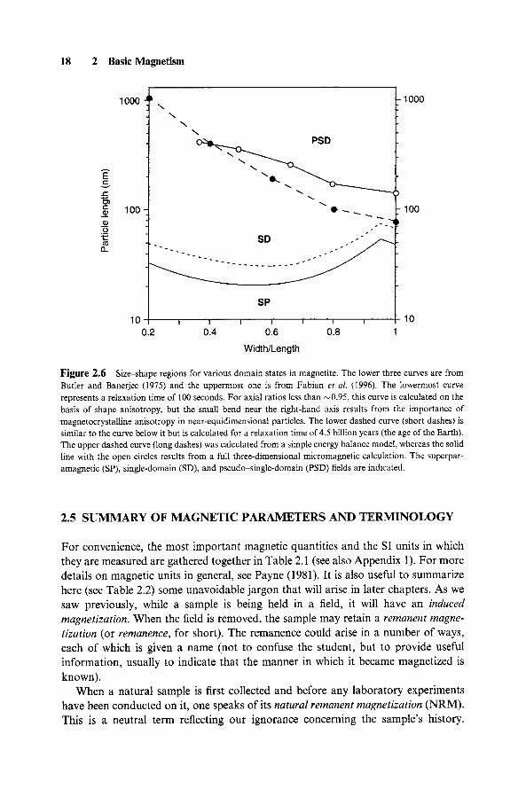
The analysis of hysteresis properties has been extended by measuring the M(H) curve not only in one major hysteresis cycle between a large positive and a large negative field. Saturating in a positive field and then reversing the field to a number of negative field values and subsequently returning to positive saturation produces a number of curves which have been named first-order reversal curves (FORCs) (Mayergoyz, 1986). They are generally transformed for better visualization into contour plots known as FORC diagrams (Pike et al., 1999; Roberts et al., 2000).

As Pike and Marvin (2001) explain, FORC measurements start out by saturating a sample in a strong positive field. Then the field is changed to a negative field Hr (Fig. 2.9a). A FORC is measured when reverting back from Hr to full positive saturation. The magnetization at the applied field Ha on the FORC with reversal field Hr is denoted by M ( H r , Ha), where Ha > Hr. The difference between successive FORCs arises from irreversible magnetization changes that occur between successive reversal fields (Fig. 2.9b). The FORC distribution is defined as the mixed second derivative:

O2M(Hr, Ha) p(Hr, Ha) = , (2.7)

aHraHa


A M (Am 2) Hsa t -----> (a) l - - - - -

"/ "a/ H r / --~,11 ~ "/- " M(Hr'Ha),

, I

-200 I / 200 (mT) /10 H

(b) M (Am 2) (C) M (Am 2)

,oo (d) P0Hr , # p0Hu

50

-200 -100 \6, ~

\z Oo/j

Ha

::::::::::::::::::::::::::::::::: U0Hc '

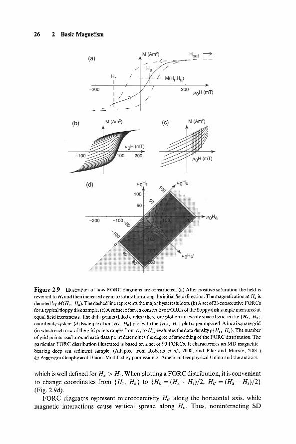
Figure 2.9 Illustration of how FORC diagrams are constructed. (a) After positive saturation the field is reversed to Hr and then increased again to saturation along the initial field direction. The magnetization at Ha is denoted by M(Hr, Ha). The dashed line represents the major hysteresis loop. (b) A set of 33 consecutive FORCs for a typical floppy disk sample. (c) A subset of seven consecutive FORCs of the floppy disk sample measured at equal field increments. The data points (filled circles) therefore plot on an evenly spaced grid in the { Hr, Ha } coordinate system. (d) Example of an { Hr, Ha } plot with the { Hc,, Hu } plot superimposed. A local square grid (in which each row of the grid points ranges from Hr to Ha) evaluates the data density p{ Hr, Ha }. The number of grid points used around each data point determines the degree of smoothing of the FORC distribution. The particular FORC distribution illustrated is based on a set of 99 FORCs. It characterizes an MD magnetite- bearing deep sea sediment sample. (Adapted from Roberts et al., 2000, and Pike and Marvin, 2001.) �9 American Geophysical Union. Modified by permission of American Geophysical Union and the authors.

which is well defined for Ha > Hr. When plotting a FORC distribution, it is convenient to change coordinates from {Hr, Ha} to {Hu = (Ha + Hr)/2, Hc' = (Ha - Hr)/2} (Fig. 2.9d).

FORC diagrams represent microcoercivity He, along the horizontal axis, while magnetic interactions cause vertical spread along Hu. Thus, noninteracting SD

2.7 Magnetic Units 27

10 I-- E

v

0 "1- o

- 1 0

0 40 80 120

PoHc,(mT)

Figure 2.10 Example of a FORC diagram of weakly interacting SD titanomagnetite from the Yucca Mountain ash flow (southern Nevada). Note that contours center around a well-defined coercivity maximum of ~45 mT and do not reach the ordinate. Vertical spread is minimal. (Adapted from Pike and Marvin, 2001, with permission of the authors.)

particles produce horizontally elongated contour lines on a FORC diagram, peaking at the appropriate Hc, with little vertical spread (Fig. 2.10). They have no contours close to the ordinate. Thermal relaxation of SP and (small) SD particles yields maximum density of vertical contour lines near Hc, = 0 (Pike et al., 2001a). MD grains seem to have vertical contour lines centered on their Hc, with a contour density spread over a comparatively large Hu interval because the domains within MD particles interact with each other (Pike et al., 2001b). Often they form contour line patches that are shaped like acute triangles in various attitudes (Roberts et al., 2000).

Loess/paleosol samples from Moravia show distinctly different FORC distributions (van Oorschot et al., 2002). The paleosol sample (Fig. 2.11, upper panel) is dominated by well-dispersed fine-grained SD magnetite grains that have a wide range of coercivities (up to 50 mT) with very little vertical spread (within + 2 mT) indicating virtually no interaction. Increased contour density close to the ordinate might indicate the presence of SP material. A few triangular contours point to the subordinate presence of MD grains. The loess sample (Fig. 2.11, lower panel) also contains SD magnetite, which is centered more to the left, indicating slightly coarser grain size. The vertical distribution is wider (most contours within + 4 mT), and more contours of MD-like triangular shape are observed. Thus, MD contributions seem to be more significant in the loess sample. SP grains cannot be discerned in the weakly magnetic loess sample.

At present, FORC diagrams are able to recognize magnetic interactions qualita- tively and to identify SP, SD, and MD particles of magnetic minerals that may constitute a complex magnetic rock mineralogy. According to Pike et al. (2001b), quantitative tools for interpreting and modeling FORC diagrams can be expected to improve these capabilities in the near future.

2.7 MAGNETIC UNITS

So far, so good. The required magnetic parameters have been successfully introduced. But because we will need to discuss real data resulting from actual laboratory


20

10

E "-' 0 i =

=s -10

-20

20

10

I -

E '-" 0 := "1- =s

-10

-20

0 20 40 60 80

-0

(D 0

0

F" 0 0 O0

0 10 20 30 40 50

,uoH c, [mT]

Figure 2.11 FORC diagram of a paleosol and a loess sample from Moravia (from van Oorschot et al., 2002). The maximum field for both diagrams was 500mT, and 106 FORCs were measured. Further explanation is given in the text. (From van Oorschot et al., 2002.) �9 Blackwell Publishing, with permission of the publishers and the authors.

investigations, we must now take a brief detour concerning the matter of units. Over the last 200 years or so, several measurement systems have been devised leading to different units being used to measure the same physical quantities: kilometers versus miles, pounds versus kilograms, and joules versus calories are familiar examples.

Nowhere has the confusion been more troublesome than in the treatment of magnet-

ism. At least four systems have been in use at various times, and the modern reader

requires conversion tables to use the older literature (e.g., see Appendix 1). No purpose

would be served in dwelling here on the fundamental reasons behind this complexity

(for a particularly lucid discussion, see Feynman e t a l . , 1964). Our sole purpose is to

introduce the system universally employed by enviromagnetic practitioners.

In this book, we stick to the Syst6me Internationale (SI, for short), which is now

taught in all high schools. Even so, a complication arises because there are two kinds

of magnetic field, H and B. The H field we have already seen in Fig. 2.1. It is measured in A/m. In the absence of matter (i.e., in a vacuum), the two fields are

related by

B - #0 H (2.8)

2.8 Putting It All Together 29

where #0 is the so-called permeability constant. In SI, it has the value 4"rr x 10 -7 Vs/Am, which means that B not only differs from H in size but also is measured in different units, namely Vs/m 2, or tesla (T) (Nikola Tesla, 1856-1943). Human nature being what it is, even the experts often do not distinguish between B and H. Indeed, for many purposes it is enough simply to refer to the "magnetic field" (you will find many examples throughout this book!). (Perhaps this laziness can be excused--after all, it is very common to give one's weight in kilograms rather than the correct SI unit of force, the newton.) Strictly speaking, of course, B and H should not be mixed up: some authors therefore refer to H as the magnetizing field and B as the magnetic induction or flux density. The Earth's magnetic B field has a strength of

5 x 10 -5 T, and a typical magnet for holding notes on your refrigerator door has a field of ~ 10 -2 T. Because the tesla is a large unit, it is common to give laboratory fields in millitesla (1 mT = 10 -3 T).

2.8 P U T T I N G IT ALL T O G E T H E R

The various enviromagnetic parameters (and their combinations) discussed here are generally employed for the purpose of answering three broad questions:

�9 Composition (i.e., which magnetic minerals are present?) �9 Concentration (i.e., how much of each one is present?) �9 Granulometry (i.e., what are the dominant grain sizes present?)

Variations in each of these offer useful information concerning environmental change, several examples of which are described in Chapter 4.

As far as composition is concerned, the most useful parameter mentioned so far is the S-ratio. But there are other important diagnostic tests, such as the Curie point and the so-called Verwey and Morin transitions. These are covered in Chapter 3, where the main features of the important environmental magnetic minerals are summarized. Several nonmagnetic techniques are also of great value in this context, including X-ray diffraction, M6ssbauer spectroscopy, and microscopy (both optical and electron).

Concentration-dependent parameters include • SIRM, and Ms. These increase monotonically with the amount of magnetic material present. They can therefore signal increases and decreases of magnetic influx into an area, perhaps as a result of changes in climate (see Chapter 7), subsurface fluid flow (see Chapter 8), biological activity (see Chapter 9), or industrial pollution (see Chapter 10). However, most parameters, other than Ms, are also dependent on grain size. This difficulty provides the motivation for the use of certain biparametric ratios that attempt to take account of variations in the total amount of magnetic material present. Successful removal of concentration dependence then emphasizes the role of grain size.

The ratio of ARM susceptibility to low-field susceptibility is one of the most widely used concentration-independent parameters. As pointed out earlier, for magnetite, XARM is strongly size dependent whereas Xlf lies close to 6 x 10 -4 m3/kg


( = 3.1 SI) over a very wide range of sizes, from 0.01 Ixm all the way up to 6 mm (Heider et al., 1996). Only as the superparamagnetic range is entered does systematic change occur (when the driving frequency of the measuring instrument becomes comparable to the relaxation times of the magnetic particles in the sample; see Eq. (2.6) and the description of susceptibility instruments in Chapter 4). At this point the susceptibility increases abruptly by an order of magnitude. For this reason, Maher (1988) recommends an experimental sequence in which the frequency dependence of the material under investigation is measured first, to check for the presence of grains near the SD/SP threshold. Then XARM is determined and normalized to remove the concentration effect. This is usually done using • as the denominator (corresponding to the King plot), although Maher herself prefers to divide by SIRM.

Engineering

Magnetismo basico