Embed Size (px)
Citation preview
MATLAB MODELLING OF SPT AND GRAIN SIZE DATA IN PRODUCING SOIL PROFILE
CE 400: PROJECT AND THESIS
Submitted by-Debojit Sarker
Student ID: 0704015
Supervised by-Dr. Md. Zoynul Abedin
Professor,Department of Civil Engineering,
BUET.
Objectives:
To develop a MATLAB computer model that could
produce the soil-profile at a particular location using GPS
coordinates or chainage location.
To validate the model using known soil profile data.
To use predicted borehole log in case studies of designing
practical problems (e.g. Pile Capacity and Liquefaction).
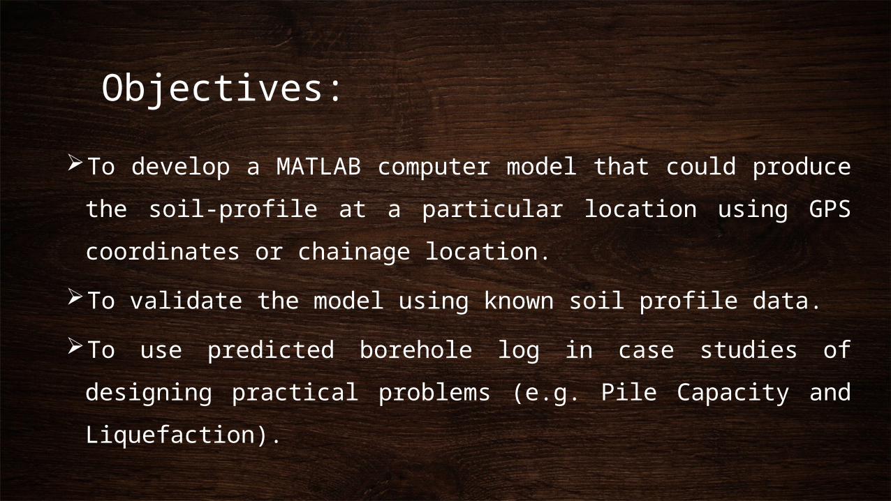
Project Site
Jajira Approach Road of Padma Multipurpose Bridge Project in Madaripur district
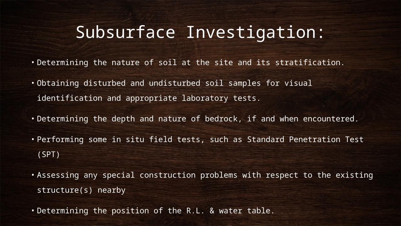
Subsurface Investigation:
• Determining the nature of soil at the site and its stratification.
• Obtaining disturbed and undisturbed soil samples for visual identification and
appropriate laboratory tests.
• Determining the depth and nature of bedrock, if and when encountered.
• Performing some in situ field tests, such as Standard Penetration Test (SPT)
• Assessing any special construction problems with respect to the existing
structure(s) nearby
• Determining the position of the R.L. & water table.
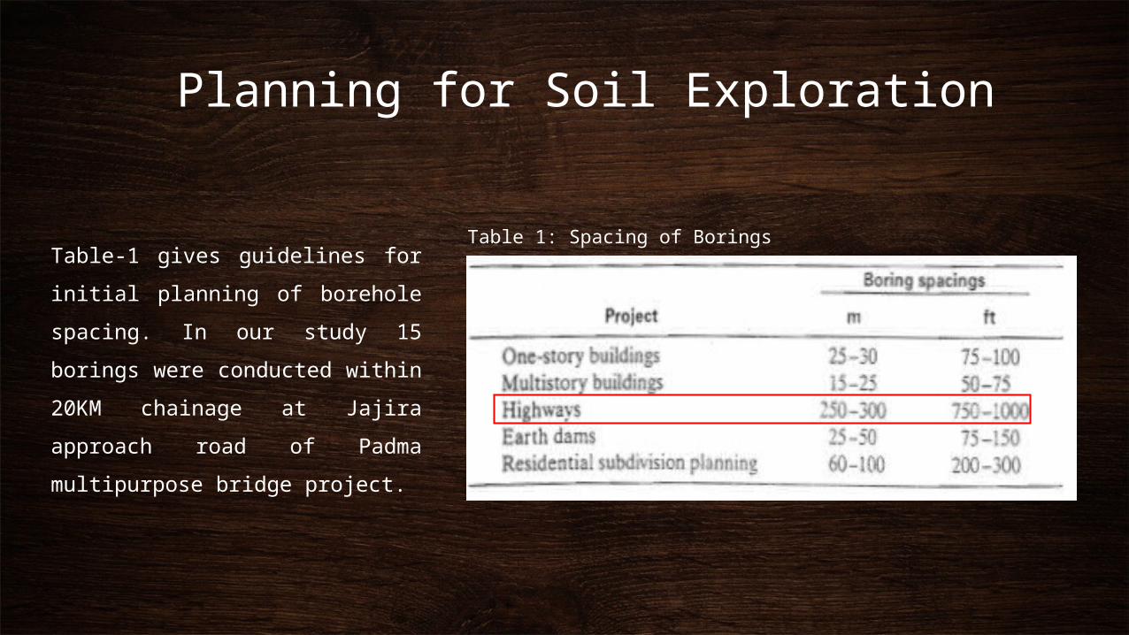
Planning for Soil Exploration
Table-1 gives guidelines for initial
planning of borehole spacing. In
our study 15 borings were
conducted within 20KM chainage
at Jajira approach road of Padma
multipurpose bridge project.
Table 1: Spacing of Borings
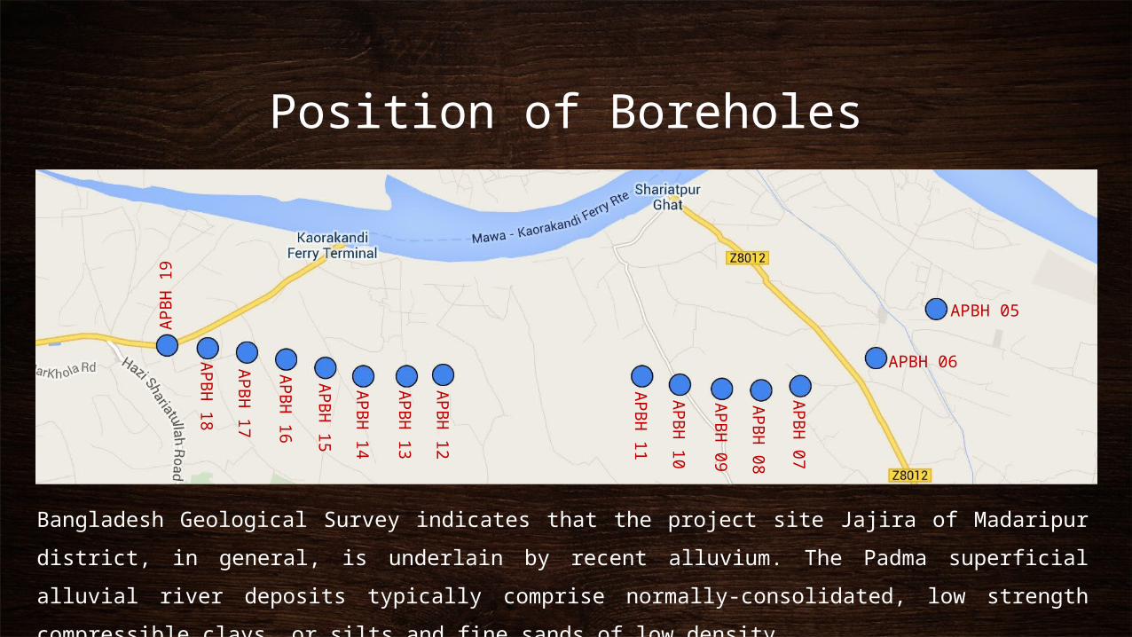
Position of Boreholes
APBH 05
APBH 06
APB
H 0
7
APB
H 0
8
APB
H 0
9
APB
H 1
0
APB
H 1
1
APB
H 1
2
APB
H 1
3
APB
H 1
4
APB
H 1
5
APB
H 1
6
APB
H 1
7
APB
H 1
8
APB
H 1
9
Bangladesh Geological Survey indicates that the project site Jajira of Madaripur district, in
general, is underlain by recent alluvium. The Padma superficial alluvial river deposits typically
comprise normally-consolidated, low strength compressible clays, or silts and fine sands of low
density.
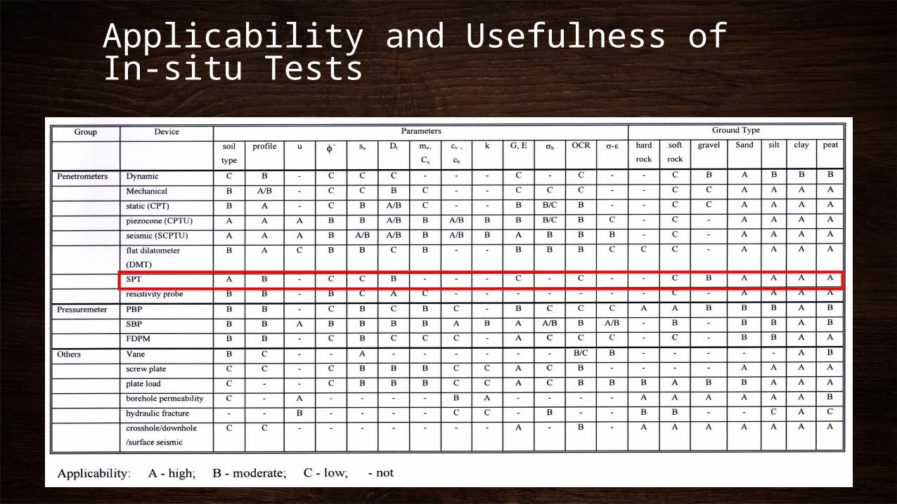
Applicability and Usefulness of In-situ Tests
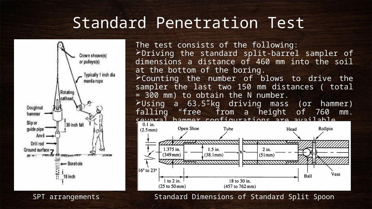
Standard Penetration TestThe test consists of the following:Driving the standard split-barrel sampler of dimensions a distance of 460 mm into the soil at the bottom of the boring.Counting the number of blows to drive the sampler the last two 150 mm distances ( total = 300 mm) to obtain the N number. Using a 63.5-kg driving mass (or hammer) falling “free” from a height of 760 mm. several hammer configurations are available.
Standard Dimensions of Standard Split SpoonSPT arrangements
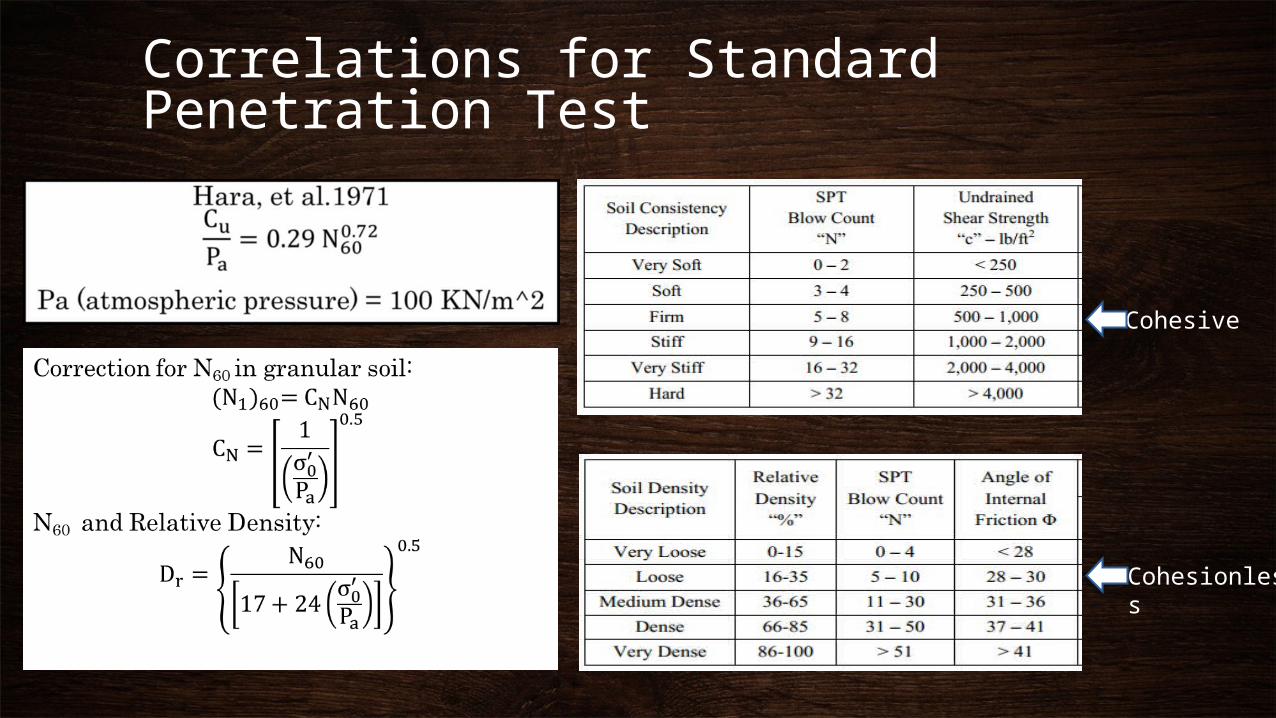
Correlations for Standard Penetration Test
Cohesive
Cohesionless
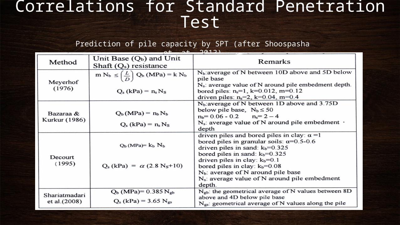
Correlations for Standard Penetration TestPrediction of pile capacity by SPT (after Shoospasha et. at. 2013)
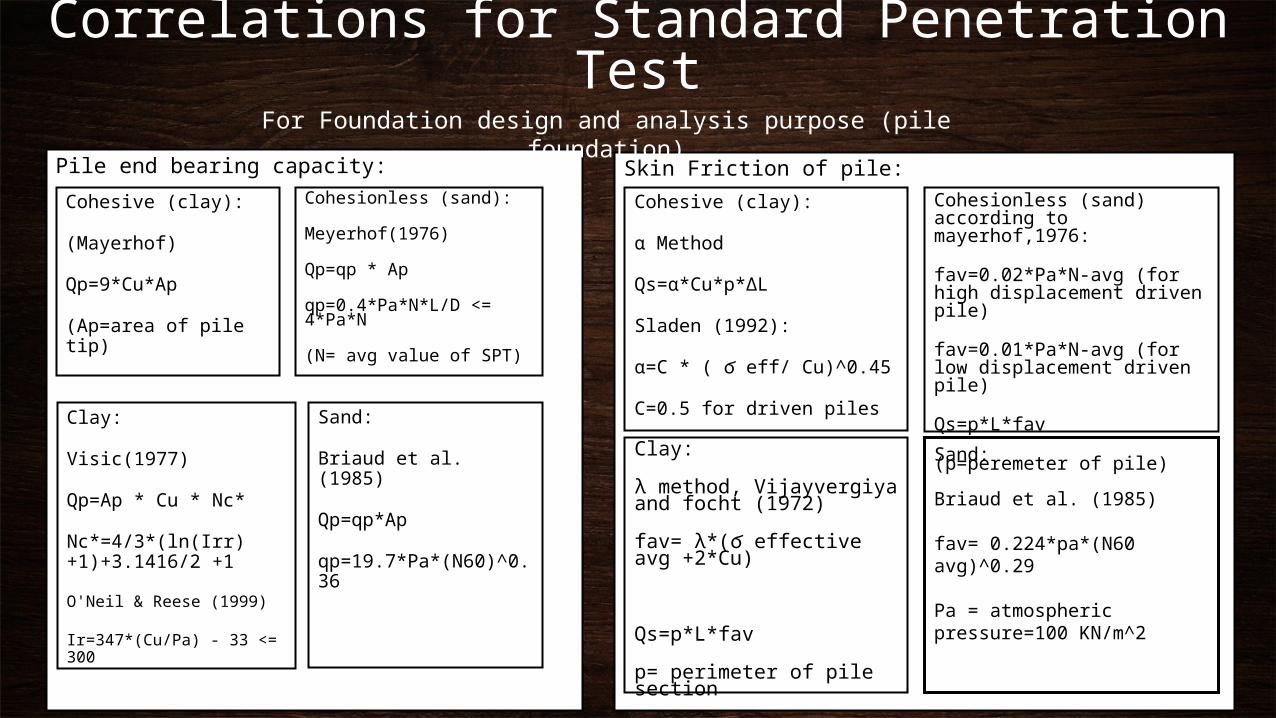
Correlations for Standard Penetration Test
Skin Friction of pile:
Cohesive (clay):
α Method
Qs=α*Cu*p*ΔL
Sladen (1992):
α=C * ( ϭ eff/ Cu)^0.45
C=0.5 for driven piles
Cohesionless (sand) according to mayerhof,1976:
fav=0.02*Pa*N-avg (for high displacement driven pile)
fav=0.01*Pa*N-avg (for low displacement driven pile)
Qs=p*L*fav
(p=peremeter of pile)
Pile end bearing capacity:
Cohesive (clay):
(Mayerhof)
Qp=9*Cu*Ap
(Ap=area of pile tip)
Cohesionless (sand):
Meyerhof(1976)
Qp=qp * Ap
qp=0.4*Pa*N*L/D <= 4*Pa*N
(N= avg value of SPT)
For Foundation design and analysis purpose (pile foundation)
Clay:
Visic(1977)
Qp=Ap * Cu * Nc*
Nc*=4/3*(ln(Irr) +1)+3.1416/2 +1
O'Neil & Reese (1999)
Ir=347*(Cu/Pa) - 33 <= 300
Sand:
Briaud et al. (1985)
Qp=qp*Ap
qp=19.7*Pa*(N60)^0.36
Clay:
λ method, Vijayvergiya and focht (1972)
fav= λ*(ϭ effective avg +2*Cu)
Qs=p*L*fav
p= perimeter of pile section
Sand:
Briaud et al. (1985)
fav= 0.224*pa*(N60 avg)^0.29
Pa = atmospheric pressure=100 KN/m^2
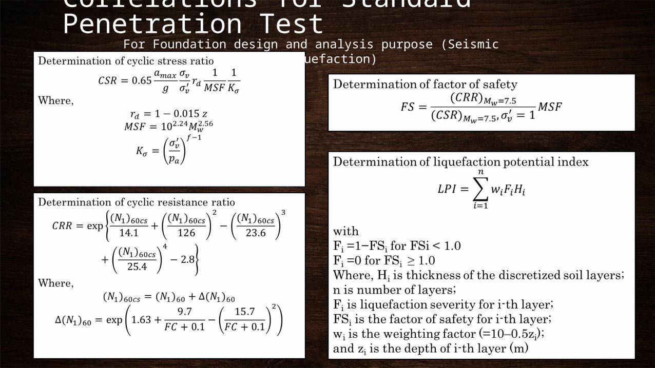
Correlations for Standard Penetration Test
For Foundation design and analysis purpose (Seismic Soil Liquefaction)
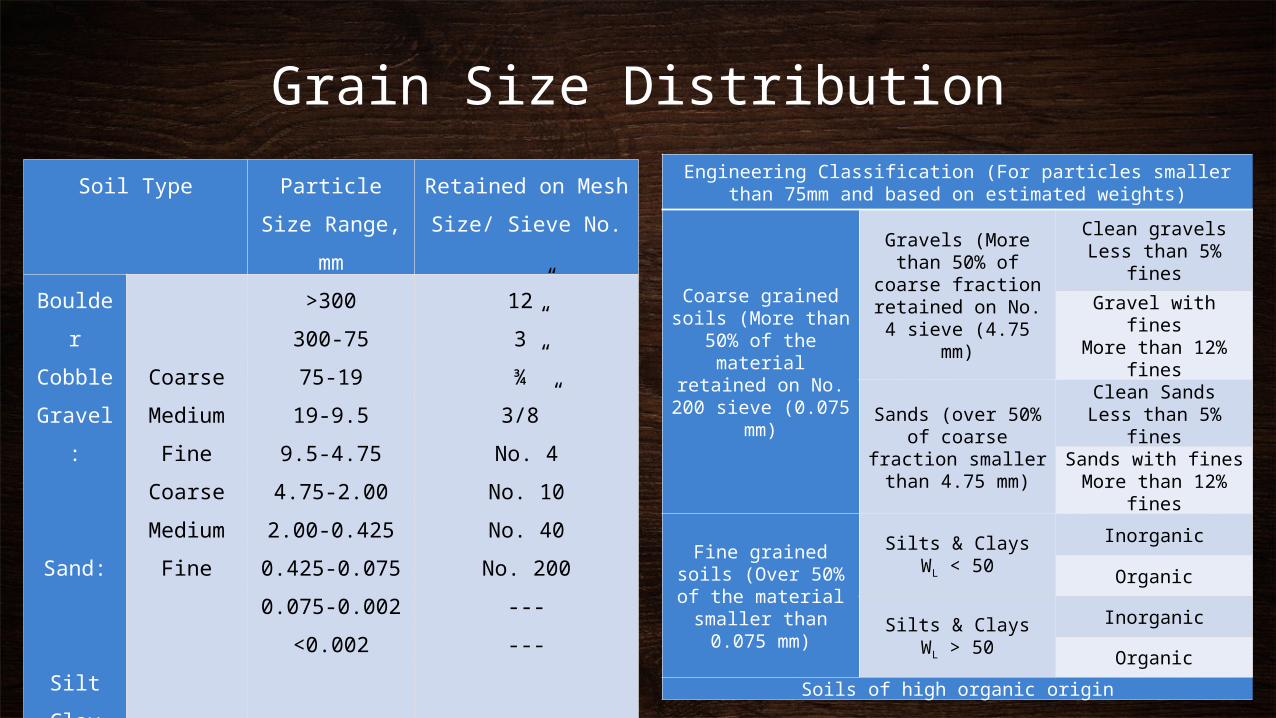
Grain Size Distribution
Soil Type Particle Size
Range, mm
Retained on Mesh
Size/ Sieve No.
Boulder
Cobble
Gravel:
Sand:
Silt
Clay
Coarse
Medium
Fine
Coarse
Medium
Fine
>300
300-75
75-19
19-9.5
9.5-4.75
4.75-2.00
2.00-0.425
0.425-0.075
0.075-0.002
<0.002
12”
3”
¾”
3/8”
No. 4
No. 10
No. 40
No. 200
---
---
Engineering Classification (For particles smaller than 75mm and based on estimated weights)
Coarse grained soils (More than
50% of the material retained on No. 200 sieve
(0.075 mm)
Gravels (More than 50% of coarse
fraction retained on No. 4 sieve
(4.75 mm)
Clean gravelsLess than 5% fines
Gravel with finesMore than 12%
fines
Sands (over 50% of coarse fraction smaller than 4.75
mm)
Clean SandsLess than 5% fines
Sands with finesMore than 12%
fines
Fine grained soils (Over 50% of the material smaller than 0.075 mm)
Silts & ClaysWL < 50
Inorganic
Organic
Silts & ClaysWL > 50
Inorganic
Organic
Soils of high organic origin
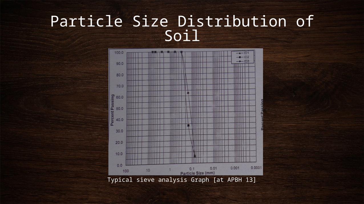
Particle Size Distribution of Soil
Typical sieve analysis Graph [at APBH 13]

MATLAB
MATLAB® is a high-level language and interactive environment
for numerical computation, visualization, and programming.
Using MATLAB, you can analyze data, develop algorithms, and
create models and applications.
The language, tools, and built-in math functions enable you to
explore multiple approaches and reach a solution faster than
with spreadsheets or traditional programming languages, such as
C/C++ or Java™.
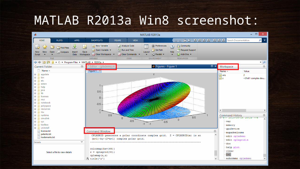
MATLAB R2013a Win8 screenshot:
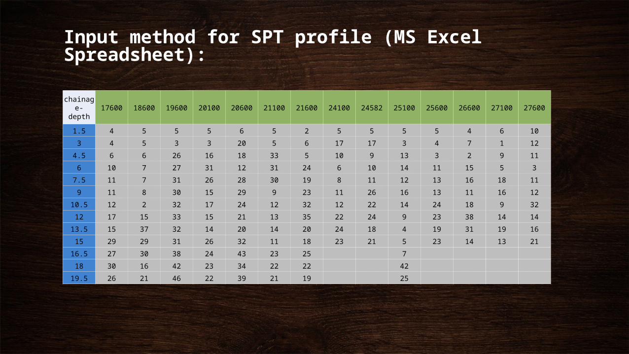
Input method for SPT profile (MS Excel Spreadsheet):
chainage- depth
17600 18600 19600 20100 20600 21100 21600 24100 24582 25100 25600 26600 27100 27600
1.5 4 5 5 5 6 5 2 5 5 5 5 4 6 10
3 4 5 3 3 20 5 6 17 17 3 4 7 1 12
4.5 6 6 26 16 18 33 5 10 9 13 3 2 9 11
6 10 7 27 31 12 31 24 6 10 14 11 15 5 3
7.5 11 7 31 26 28 30 19 8 11 12 13 16 18 11
9 11 8 30 15 29 9 23 11 26 16 13 11 16 12
10.5 12 2 32 17 24 12 32 12 22 14 24 18 9 32
12 17 15 33 15 21 13 35 22 24 9 23 38 14 14
13.5 15 37 32 14 20 14 20 24 18 4 19 31 19 16
15 29 29 31 26 32 11 18 23 21 5 23 14 13 21
16.5 27 30 38 24 43 23 25 7
18 30 16 42 23 34 22 22 42
19.5 26 21 46 22 39 21 19 25
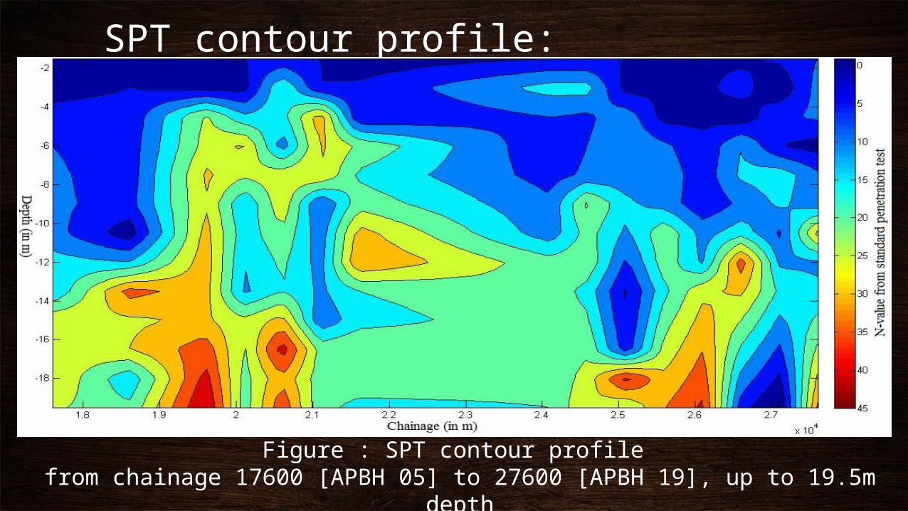
SPT contour profile:
Figure : SPT contour profile from chainage 17600 [APBH 05] to 27600 [APBH 19], up to 19.5m depth
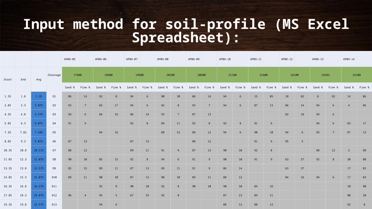
Input method for soil-profile (MS Excel Spreadsheet):
APBH-05 APBH-06 APBH-07 APBH-08 APBH-09 APBH-10 APBH-11 APBH-12 APBH-13 APBH-14
Start End Avg
Chainage 17600 18600 19600 20100 20600 21100 21600 24100 24582 25100
Sand % Fine % Sand % Fine % Sand % Fine % Sand % Fine % Sand % Fine % Sand % Fine % Sand % Fine % Sand % Fine % Sand % Fine % Sand % Fine %
1.35 1.8 1.35 D1 86 14 92 8 94 6 90 10 86 14 94 6 15 85 18 82 8 92 14 86
2.85 3.3 3.075 D2 93 7 83 17 94 6 92 8 93 7 94 6 87 13 86 14 94 6 4 96
4.35 4.8 4.575 D3 94 6 84 16 86 14 93 7 87 13 82 18 94 6
5.85 6.3 6.075 D4 91 9 92 8 89 11 92 8 92 8 91 9 94 6 83 17
7.35 7.82 7.585 D5 84 16 88 12 88 12 94 6 90 10 94 6 93 7 87 13
8.85 9.3 9.075 D6 87 13 87 13 88 12 91 9 95 5
10.35 10.8 10.575 D7 88 12 89 11 91 9 87 13 90 10 92 8 88 12 2 98
11.85 12.3 12.075 D8 90 10 85 15 92 8 94 6 91 9 90 10 91 9 63 37 92 8 20 80
13.35 13.8 13.575 D9 85 15 89 11 87 13 89 11 91 9 86 14 63 37 17 83
14.85 15.3 15.075 D10 89 11 90 10 87 13 90 10 89 11 88 12 84 16 94 6 17 83
16.35 16.8 16.575 D11 92 8 90 10 92 8 90 10 90 10 84 16 10 90
17.85 18.3 18.075 D12 96 4 95 5 67 33 92 8 87 13 89 11 90 10
19.35 19.8 19.575 D13 94 6 88 12 88 12 92 8
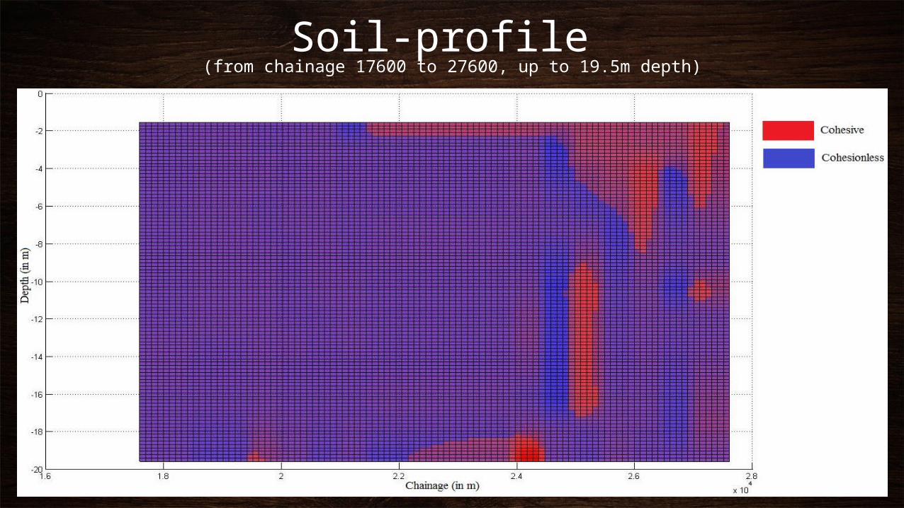
Soil-profile (from chainage 17600 to 27600, up to 19.5m depth)
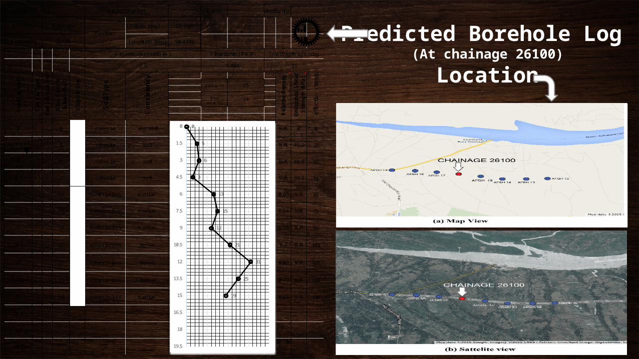
Predicted Borehole Log (At chainage 26100)
Location
Latitude (deg) 23.4009
Longitude (deg) 90.1735
0 0 cohesive very soft N/A 0 0
1.5 5 cohesive soft N/A 46.2 23
3 6 cohesive soft N/A 48.8 42
4.5 3 cohesive soft N/A 39.9 54
6 13 cohesionless medium 0.63 N/A 66
7.5 15 cohesionless medium 0.64 N/A 79
9 12 cohesionless medium 0.55 N/A 91
10.5 21 cohesionless dense 0.7 N/A 103
12 31 cohesionless dense 0.83 N/A 115
13.5 25 cohesionless dense 0.72 N/A 128
15 19 cohesionless medium 0.61 N/A 140
16.5
18
19.5
effe
ctiv
e s
tress
γ (kN/m 2̂) 15
γ sat (kN/m 2̂)
18
Rela
tive D
en
sit
y
Un
dra
ined
Sh
ear
Str
en
gth
(kP
a)
Gra
ph
ic L
og
Dep
th (
mete
r)
Sam
ple
Typ
e
Sam
ple
Nu
mb
er
Blo
w C
ou
nts
(b
low
s/f
oo
t)
So
il T
yp
e
Co
ns
iste
nc
y
Groundwater Depth (m):
2.5
Elevation(m) PWD:
5.804
Total Depth of Boring:
15
Project Number:Project: Client: Boring No.
Address: Madaripur
Position:
Chainage: 26100
0
5
6
3
13
15
12
21
31
25
19
0
1.5
3
4.5
6
7.5
9
10.5
12
13.5
15
16.5
18
19.5
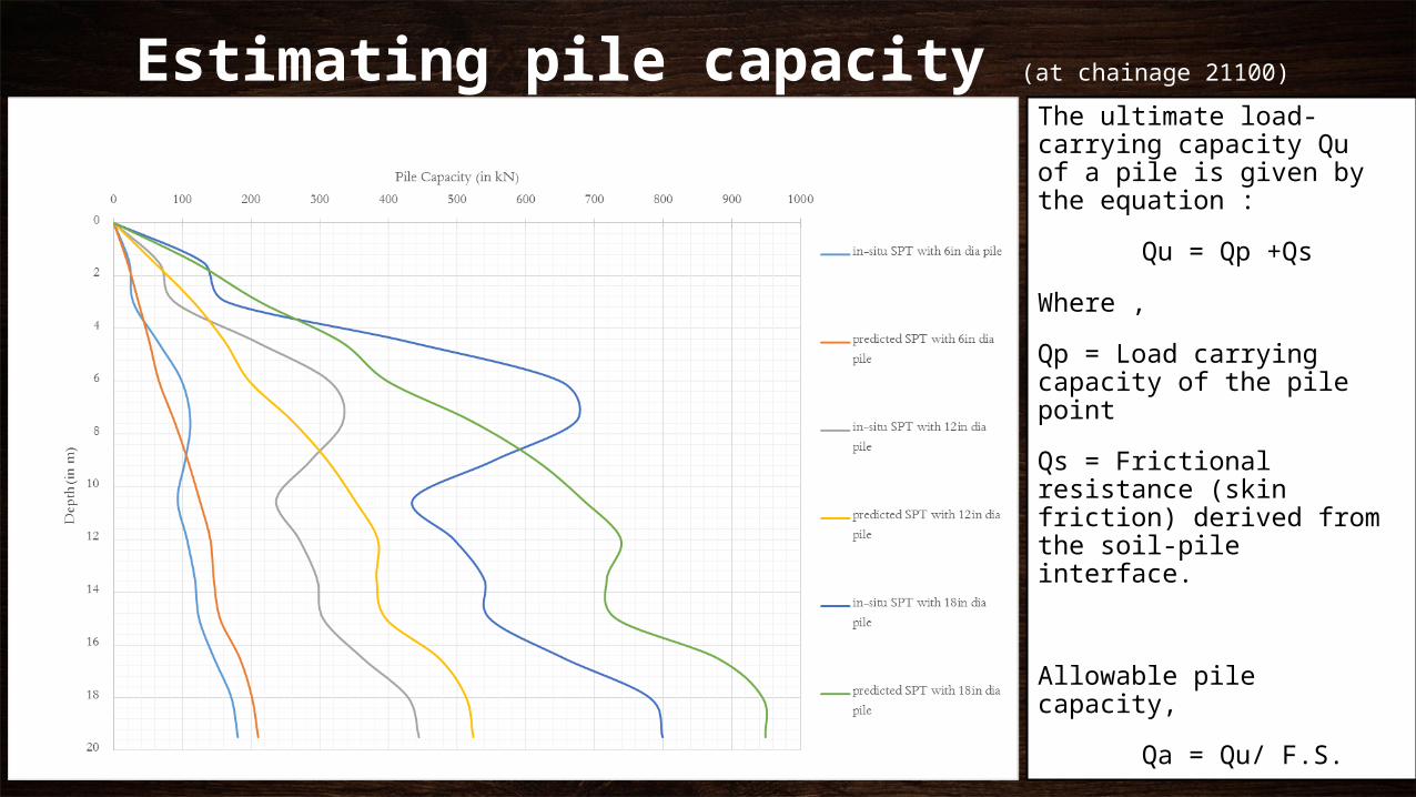
The ultimate load-carrying capacity Qu of a pile is given by the equation :
Qu = Qp +Qs
Where ,
Qp = Load carrying capacity of the pile point
Qs = Frictional resistance (skin friction) derived from the soil-pile interface.
Allowable pile capacity,
Qa = Qu/ F.S.
Estimating pile capacity (at chainage 21100)
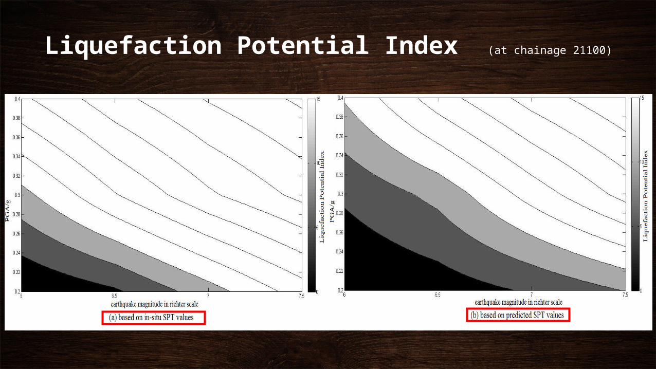
Liquefaction Potential Index (at chainage 21100)
Summary
The developed MATLAB model can predict an intermittent borehole log with
reasonable accuracy.
The developed model gives SPT contours that may be used to identify the soil
spatial stiffness.
The program yields grain size surface plots that may be used to identify the soil
profile.
The estimation of pile capacity suggests that the predicted borehole estimates the
SPT values well.
The variation in liquefaction potential suggests that the model be refined for grain
size estimation.

Thank You