Energy saving policies final

Alejandro Fernández-Montes González

Advisors: Juan Antonio Ortega

Luis González Abril

Energy-Saving Policies in

Grid-Computing and

Smart Environments

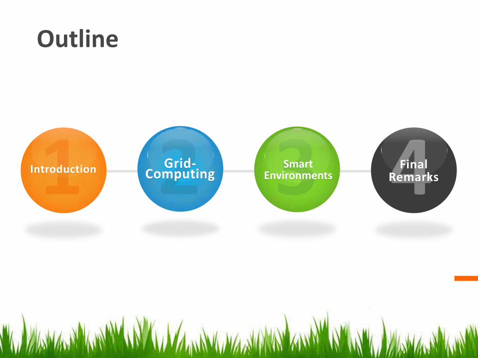
Outline

Introduction Grid-Computing

Smart Environments

FinalRemarks

Introduction Research

Motivation, Success Criteria, Energy Efficiency, Energy vs Power

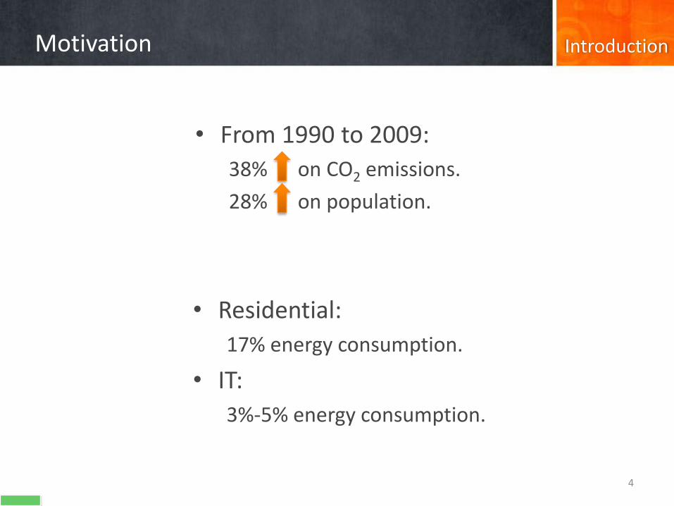
IntroductionMotivation

• From 1990 to 2009:

38% on CO2 emissions.

28% on population.

• Residential:

17% energy consumption.

• IT:

3%-5% energy consumption.

4

IntroductionResearch Question & Success criteria

5

Which are the best energy policies to save energy in Grid-Computing and Smart Environments?

• Check if both model and supporting algorithms define energy-saving policies indeed.

• Demonstrate it by experiments through simulation software.

IntroductionEnergy efficiency

6

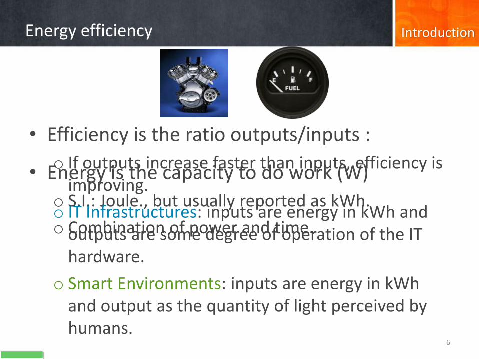
• Energy is the capacity to do work (W)

o S.I.: Joule., but usually reported as kWh.

o Combination of power and time.

• Efficiency is the ratio outputs/inputs :

o If outputs increase faster than inputs, efficiency is improving.

o IT Infrastructures: inputs are energy in kWh and outputs are some degree of operation of the IT hardware.

o Smart Environments: inputs are energy in kWh and output as the quantity of light perceived by humans.

IntroductionEnvironments analyzed

7

• Energy efficiency has been tackled from two sides:

o Grid-Computing. Collaboration with to save energy in Grid’5000 infrastructure.

o Smart Environments. Study about lighting conditions supported with sensors in order to save energy.

IntroductionThesis Outline

• Grid-Computing

o 2011

o 2012

• Smart Environments

o 2009

• Defended as a set of papers.

8

Grid-Computing Energy-Saving policies,Efficiency Comparison

Grid’5000, Simulation Software, On-off policies, Data Envelopment Analysis

Grid-ComputingData Center

10

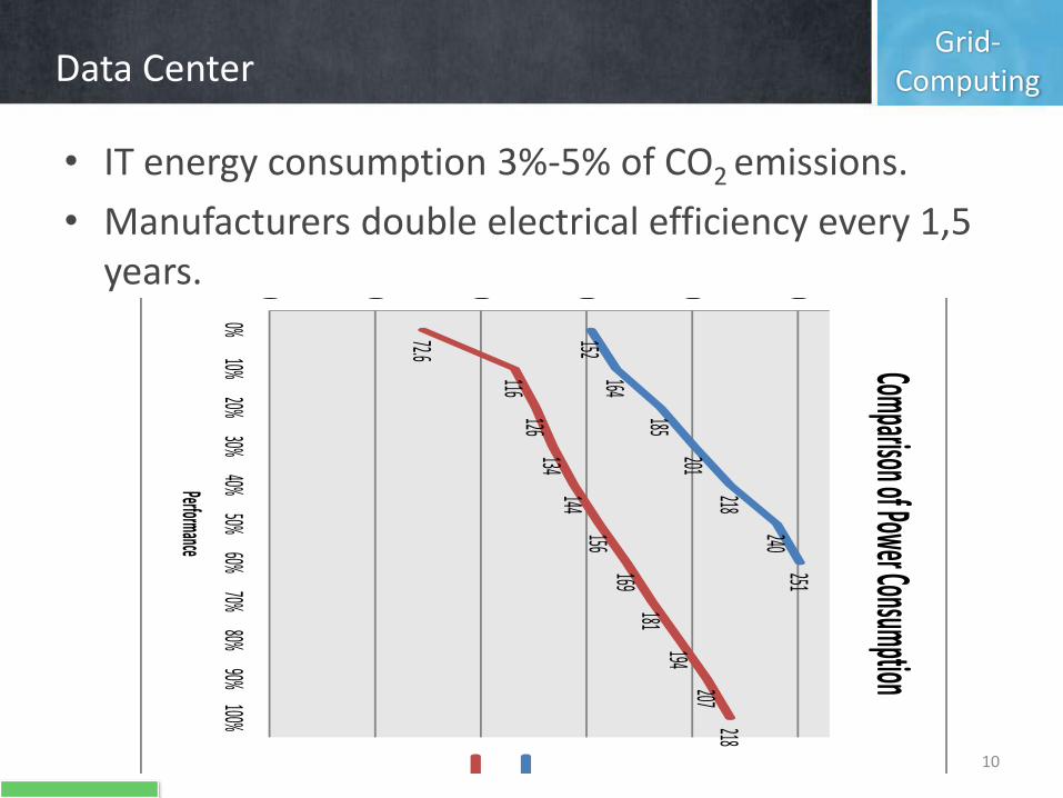
• IT energy consumption 3%-5% of CO2 emissions.

• Manufacturers double electrical efficiency every 1,5 years.

152164

185201

218

240251

72.6

116126

134144

156169

181194

207218

0 50 100 150 200 250

0%10%

20%30%

40%50%

60%70%

80%90%

100%

Power (Watts)

Performance

Comparison of Power Consumption

w2k3

w2k8

Grid-ComputingData Center

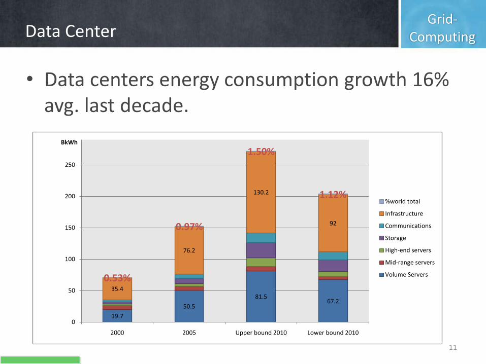
11

• Data centers energy consumption growth 16% avg. last decade.

19.7

50.5

81.567.2

35.4

76.2

130.2

92

0.53%

0.97%

1.50%

1.12%

0

50

100

150

200

250

2000 2005 Upper bound 2010 Lower bound 2010

BkWh

%world total

Infrastructure

Communications

Storage

High-end servers

Mid-range servers

Volume Servers

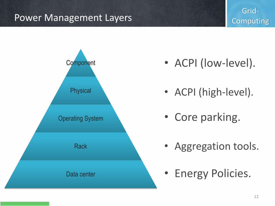
Grid-ComputingPower Management Layers

12

Component

Physical

Operating System

Rack

Data center

• ACPI (low-level).

• ACPI (high-level).

• Core parking.

• Aggregation tools.

• Energy Policies.

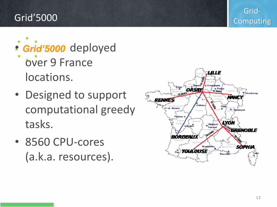
Grid-ComputingGrid’5000

13

• deployed over 9 France locations.

• Designed to support computational greedy tasks.

• 8560 CPU-cores (a.k.a. resources).

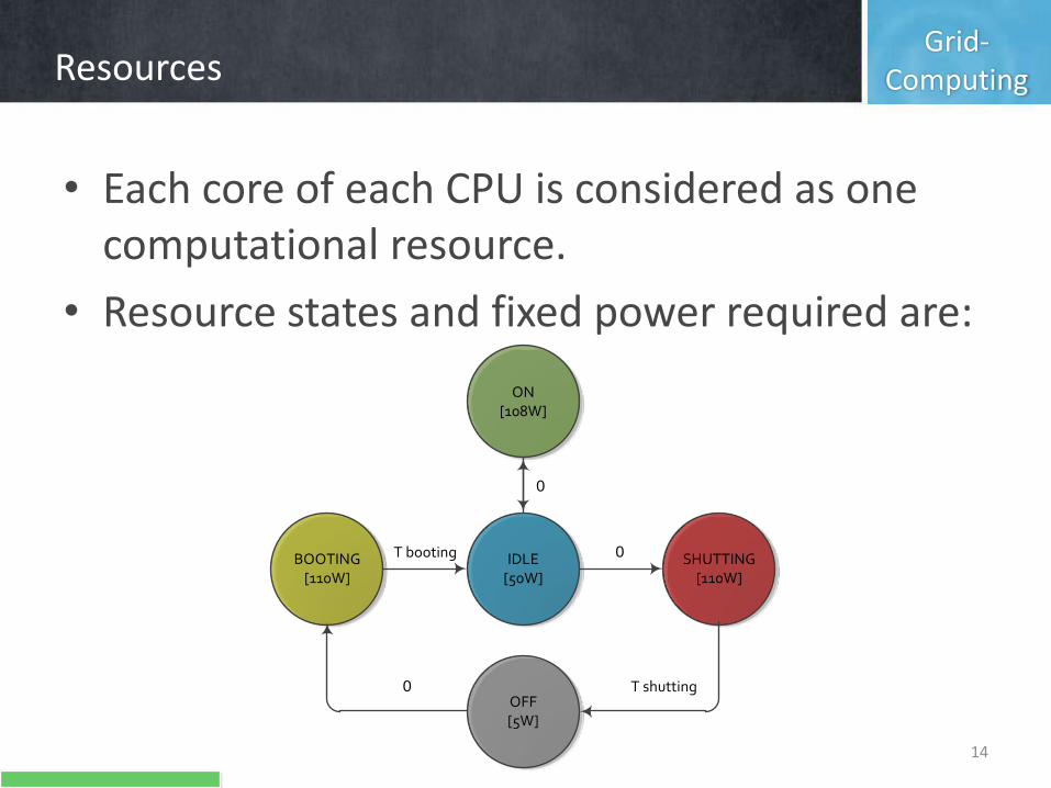
Grid-ComputingResources

14

• Each core of each CPU is considered as one computational resource.

• Resource states and fixed power required are:

IDLE[50W]

OFF[5W]

BOOTING[110W]

SHUTTING[110W]

ON[108W]

T booting

0

0

T shutting0

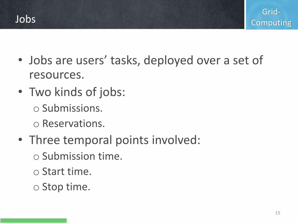
Grid-ComputingJobs

15

• Jobs are users’ tasks, deployed over a set of resources.

• Two kinds of jobs:o Submissions.

o Reservations.

• Three temporal points involved:o Submission time.

o Start time.

o Stop time.

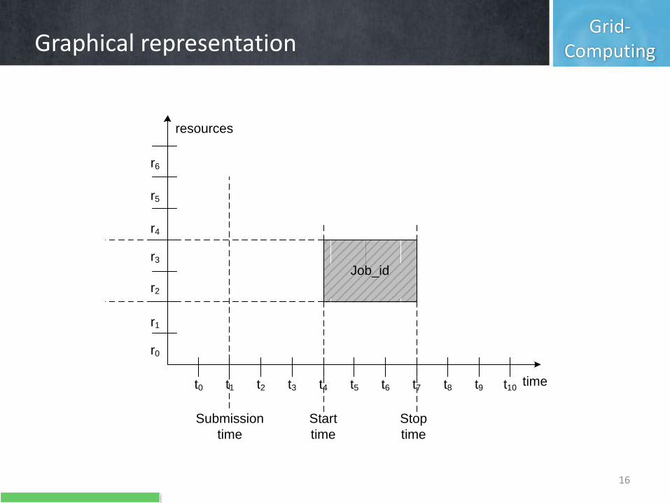
Grid-ComputingGraphical representation

16

resources

time

r0

t0

r6

r5

r4

r3

r2

r1

t8t7t6t5t4t3t2t1 t10t9

Job_id

Start

time

Stop

time

Submission

time

Grid-ComputingScheduling Energy Policies

17

• Establish the managing of the states of grid resources.

• What to do with each resource that finishes the execution of a job:

o Leave On (idle).

o Shut resource down.

• Seven energy policies proposals are analyzedand compared.

Off

Idle

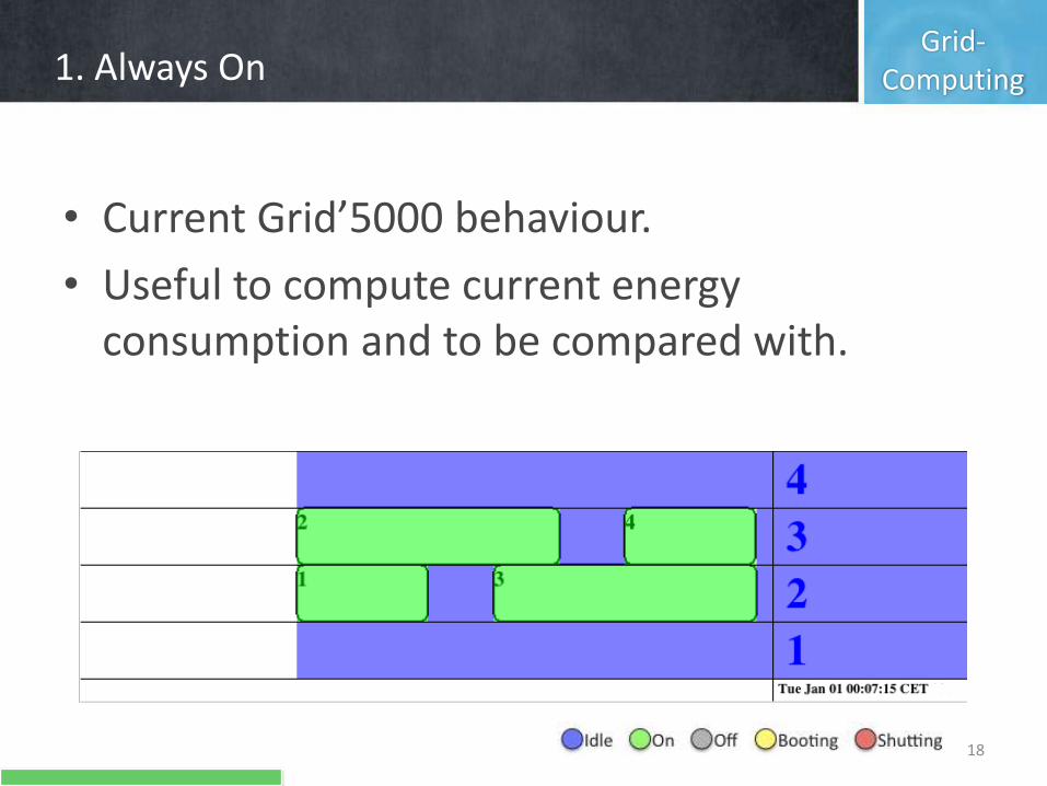
Grid-Computing1. Always On

18

• Current Grid’5000 behaviour.

• Useful to compute current energy consumption and to be compared with.

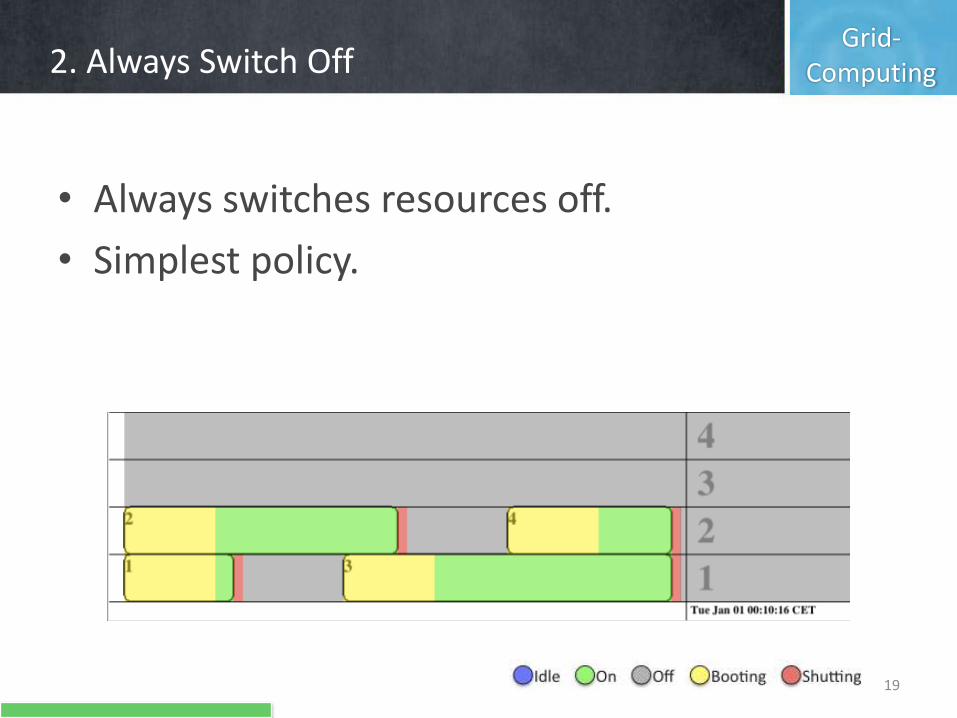
Grid-Computing2. Always Switch Off

19

• Always switches resources off.

• Simplest policy.

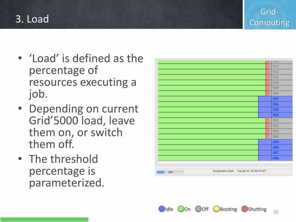
Grid-Computing3. Load

20

• ‘Load’ is defined as the percentage of resources executing a job.

• Depending on current Grid’5000 load, leave them on, or switch them off.

• The threshold percentage is parameterized.

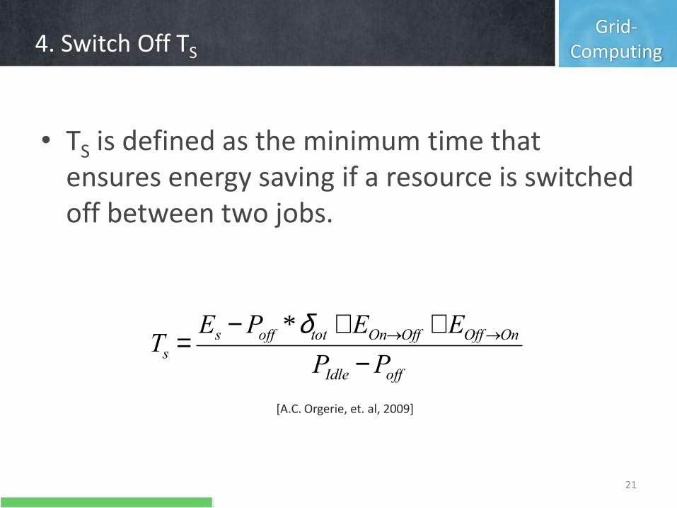
Grid-Computing4. Switch Off TS

21

• TS is defined as the minimum time that ensures energy saving if a resource is switched off between two jobs.

Ts =Es -Poff *dtot +EOn®Off +EOff®On

PIdle -Poff

[A.C. Orgerie, et. al, 2009]

Grid-Computing4. Switch Off TS

22

• Looks in the agenda for jobs that are going to be run in a period less than TS.

• Computes number of resources that are going to be needed and acts on resources.

• Only this energy policy looks up the agenda for reservations already made.

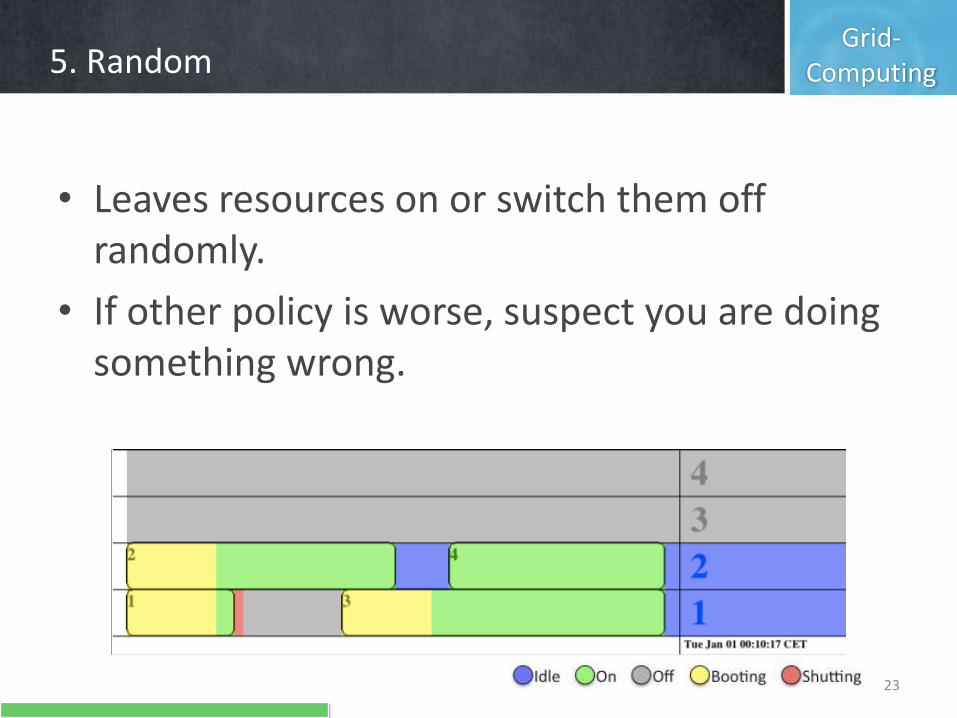
Grid-Computing5. Random

23

• Leaves resources on or switch them off randomly.

• If other policy is worse, suspect you are doing something wrong.

Grid-Computing6. Exponential

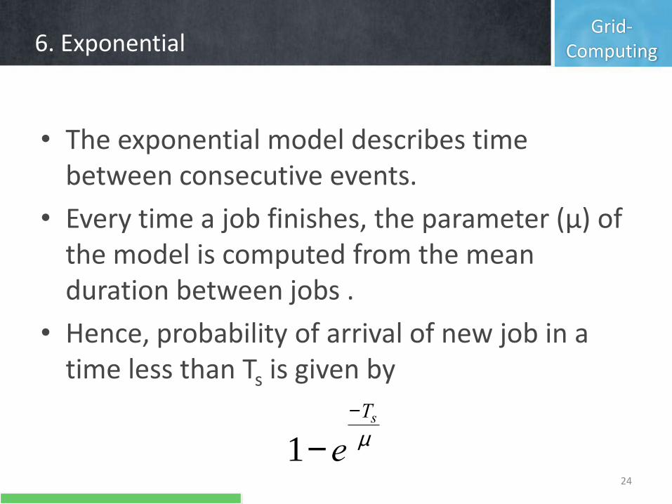
24

• The exponential model describes time between consecutive events.

• Every time a job finishes, the parameter (μ) of the model is computed from the mean duration between jobs .

• Hence, probability of arrival of new job in a time less than Ts is given by

1- e

-Ts

m

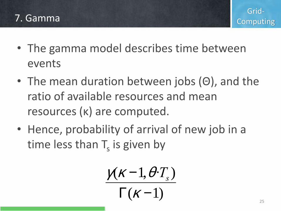
Grid-Computing7. Gamma

25

• The gamma model describes time between events

• The mean duration between jobs (Θ), and the ratio of available resources and mean resources (κ) are computed.

• Hence, probability of arrival of new job in a time less than Ts is given by

g(k -1,q ·Ts )

G(k -1)

Grid-ComputingArranging policies

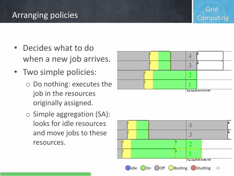
26

• Decides what to do when a new job arrives.

• Two simple policies:

o Do nothing: executes the job in the resources originally assigned.

o Simple aggregation (SA): looks for idle resources and move jobs to these resources.

Grid-ComputingExperimentation

27

• Tested all combinations of Energy and Arranging policies.

• Computed results:

o Energy consumed.

o Energy saved.

o Number of bootings and shuttings.

o Comparison between minimal and actual.

o Saved energy by booting-shutting.

Grid-ComputingExperimentation

28

• Two periods of six months.

• Seven energy policies.

Configurable energy policies have been used with various values.

• Two arranging policies.

• Add up to a total of 324 simulations.

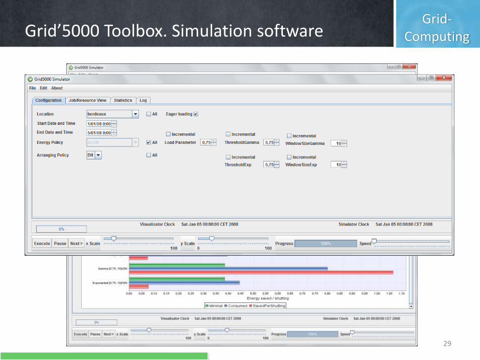
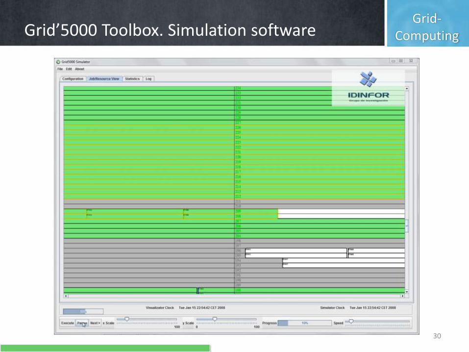
Grid-ComputingGrid’5000 Toolbox. Simulation software

29

Grid-ComputingGrid’5000 Toolbox. Simulation software

30

‹#›

‹#›

Grid-ComputingResults

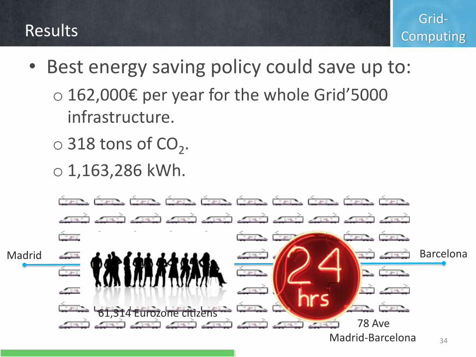
• Best energy saving policy could save up to:

o 162,000€ per year for the whole Grid’5000 infrastructure.

o 318 tons of CO2.

o 1,163,286 kWh.

Madrid Barcelona

78 Ave Madrid-Barcelona

61,314 Eurozone citizens

34

Grid-Computing

35

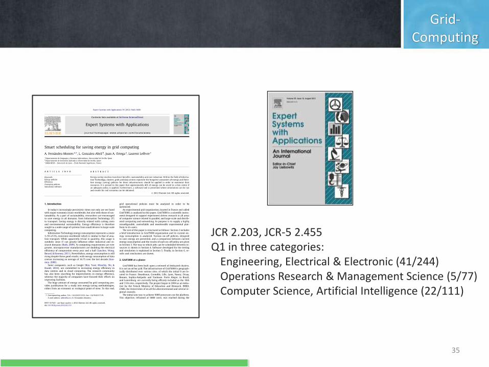
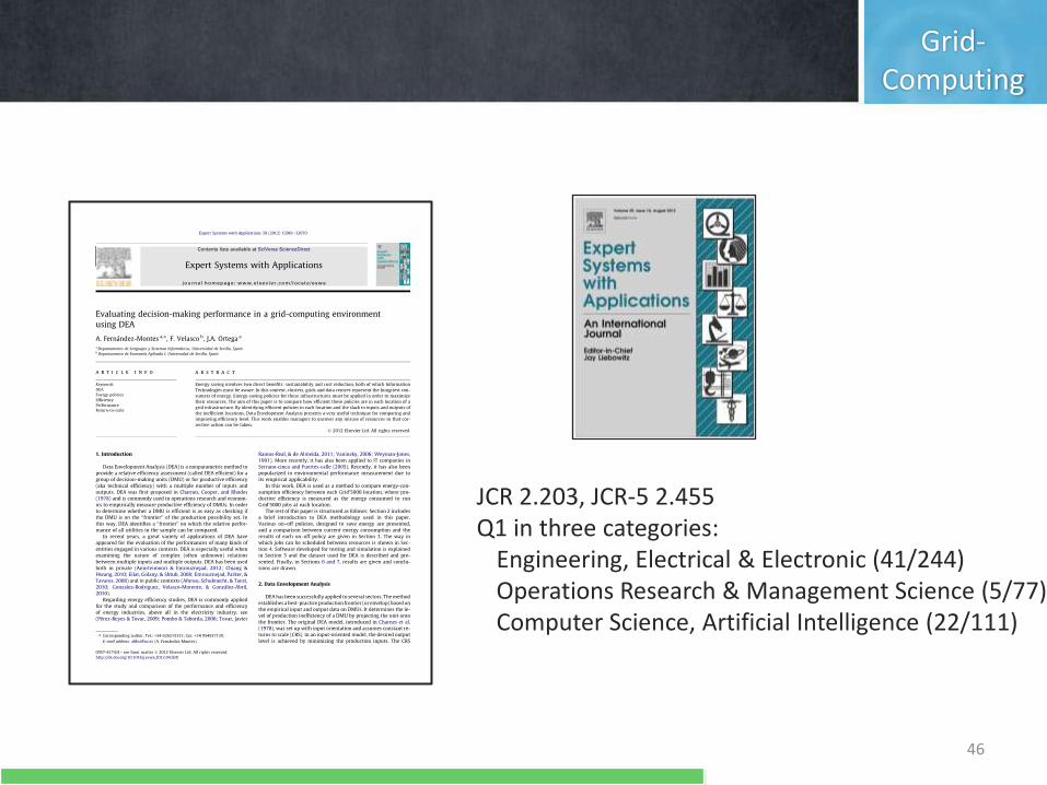
JCR 2.203, JCR-5 2.455Q1 in three categories:

Engineering, Electrical & Electronic (41/244)Operations Research & Management Science (5/77)Computer Science, Artificial Intelligence (22/111)

Grid-Computing

Efficiency Analysis. Data Envelopment Analysis (DEA)

36

• Non-parametric method to provide a relative efficiency assessment for a group of decision-making units (DMU) with multiple inputs and outputs.

• Useful to answer questions like:o Which are the most efficient franchises of a company?o What parameters should be changed in a franchise to

be more efficient?

• Establishes the efficient frontier to check if a DMU is efficient or not, and provides the actions that should be applied.

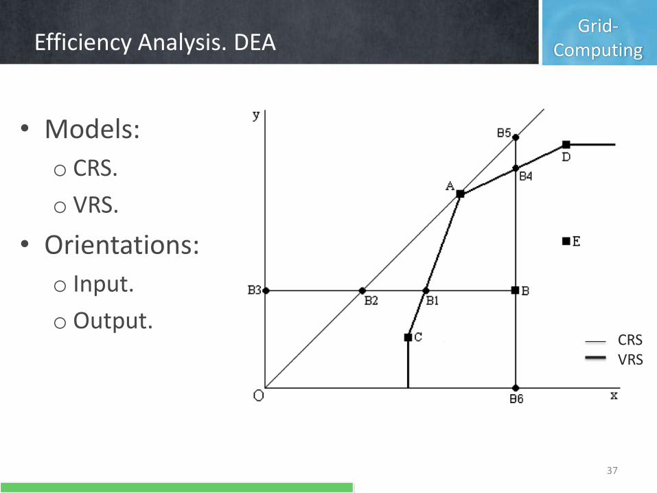
Grid-ComputingEfficiency Analysis. DEA

37

CRSVRS

• Models:

o CRS.

o VRS.

• Orientations:

o Input.

o Output.


38

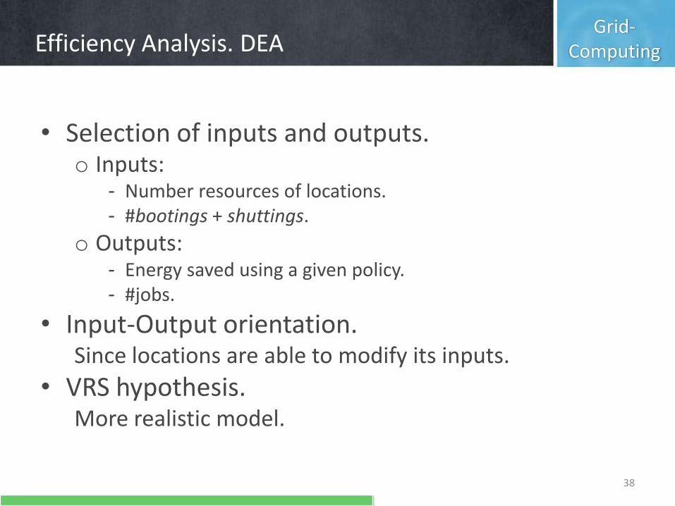
• Selection of inputs and outputs.o Inputs:

- Number resources of locations.- #bootings + shuttings.

o Outputs:- Energy saved using a given policy.- #jobs.

• Input-Output orientation.Since locations are able to modify its inputs.

• VRS hypothesis.More realistic model.


39

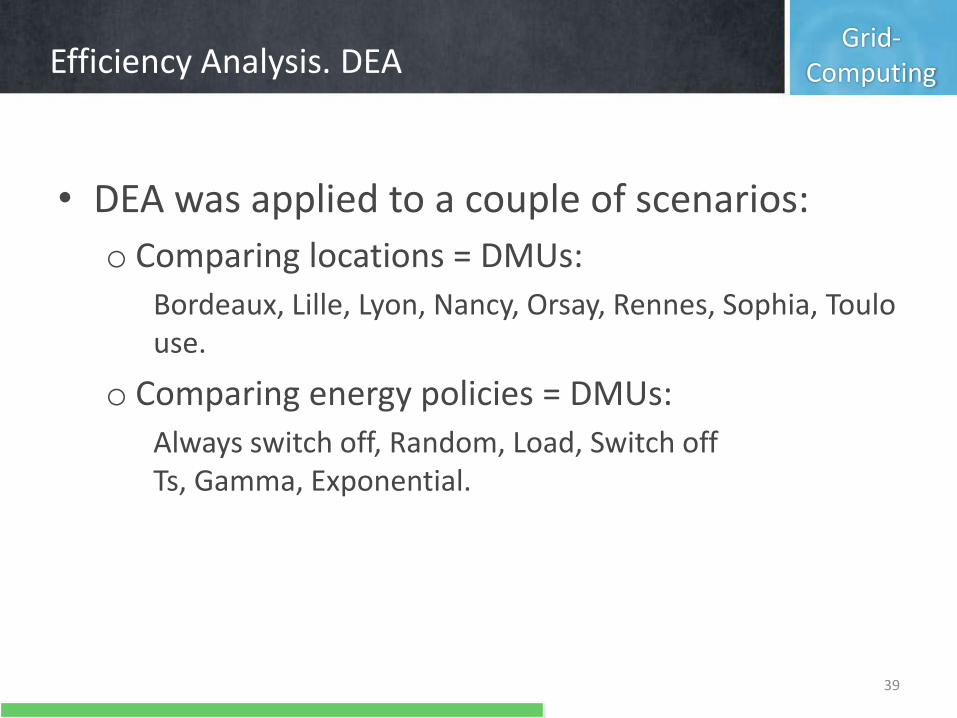
• DEA was applied to a couple of scenarios:

o Comparing locations = DMUs:

Bordeaux, Lille, Lyon, Nancy, Orsay, Rennes, Sophia, Toulouse.

o Comparing energy policies = DMUs:

Always switch off, Random, Load, Switch off Ts, Gamma, Exponential.

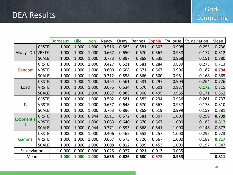
Grid-ComputingDEA Results

40

Bordeaux Lille Lyon Nancy Orsay Rennes Sophia Toulouse St. deviation Mean

Always Off

CRSTE 1.000 1.000 1.000 0.516 0.583 0.581 0.303 0.908 0.255 0.736

VRSTE 1.000 1.000 1.000 0.667 0.650 0.670 0.567 0.938 0.177 0.812

SCALE 1.000 1.000 1.000 0.773 0.897 0.868 0.535 0.968 0.151 0.880

Random

CRSTE 1.000 1.000 1.000 0.427 0.521 0.581 0.284 0.889 0.273 0.713

VRSTE 1.000 1.000 1.000 0.600 0.608 0.671 0.567 0.906 0.187 0.794

SCALE 1.000 1.000 1.000 0.712 0.858 0.866 0.500 0.981 0.168 0.865

Load

CRSTE 1.000 1.000 1.000 0.464 0.561 0.581 0.297 0.904 0.264 0.726

VRSTE 1.000 1.000 1.000 0.675 0.634 0.670 0.601 0.937 0.172 0.815

SCALE 1.000 1.000 1.000 0.687 0.885 0.868 0.495 0.965 0.171 0.862

Ts

CRSTE 1.000 1.000 1.000 0.502 0.581 0.582 0.294 0.936 0.261 0.737

VRSTE 1.000 1.000 1.000 0.657 0.648 0.670 0.567 0.937 0.178 0.810

SCALE 1.000 1.000 1.000 0.763 0.896 0.868 0.519 0.999 0.159 0.881

Exponential

CRSTE 1.000 1.000 0,944 0.511 0.572 0.581 0.307 1.000 0.259 0.739

VRSTE 1.000 1.000 1.000 0.663 0.640 0.670 0.567 1.000 0.185 0.817

SCALE 1.000 1.000 0,944 0.771 0.893 0.868 0.541 1.000 0.148 0.877

Gamma

CRSTE 1.000 1.000 1.000 0.406 0.465 0.653 0.257 1.000 0.295 0.723

VRSTE 1.000 1.000 1.000 0.667 0.573 0.726 0.567 1.000 0.189 0.817

SCALE 1.000 1.000 1.000 0.608 0.812 0.899 0.453 1.000 0.197 0.847

St. deviation 0.000 0.000 0.000 0.025 0.027 0.021 0.013 0.035

Mean 1.000 1.000 1.000 0.655 0.626 0.680 0.573 0.953 0.811

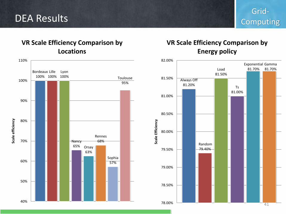
Grid-ComputingDEA Results

41

Bordeaux100%

Lille100%

Lyon100%

Nancy65% Orsay

63%

Rennes68%

Sophia57%

Toulouse95%

40%

50%

60%

70%

80%

90%

100%

110%

Scal

e e

ffic

ien

cy

VR Scale Efficiency Comparison by Locations

Always Off 81.20%

Random 79.40%

Load 81.50%

Ts 81.00%

Exponential 81.70%

Gamma 81.70%

78.00%

78.50%

79.00%

79.50%

80.00%

80.50%

81.00%

81.50%

82.00%

Scal

e E

ffic

ien

cy

VR Scale Efficiency Comparison by Energy policy

Grid-ComputingCorrections needed

42

VariableOriginal

ValueRadial

MovementSlack

movementProjected

value

Output Saved energy 152,141 0 0 152,141

Output #jobs 57,987 0 38,556 96,543

Input #resources 714 -235 0 478

Input #bootings 1,770,858 -584,429 -832,549 353,879

Rennes under the energy policy Exponential.

VariableOriginal

ValueRadial

MovementSlack

movementProjected

value

Output Saved energy 85,250 0 0 152,141

Output #jobs 165,995 0 0 165,995

Input #resources 434 -27 0 406

Input #bootings 876,026 -55,393 0 820,632

Toulouse under the energy policy TS.

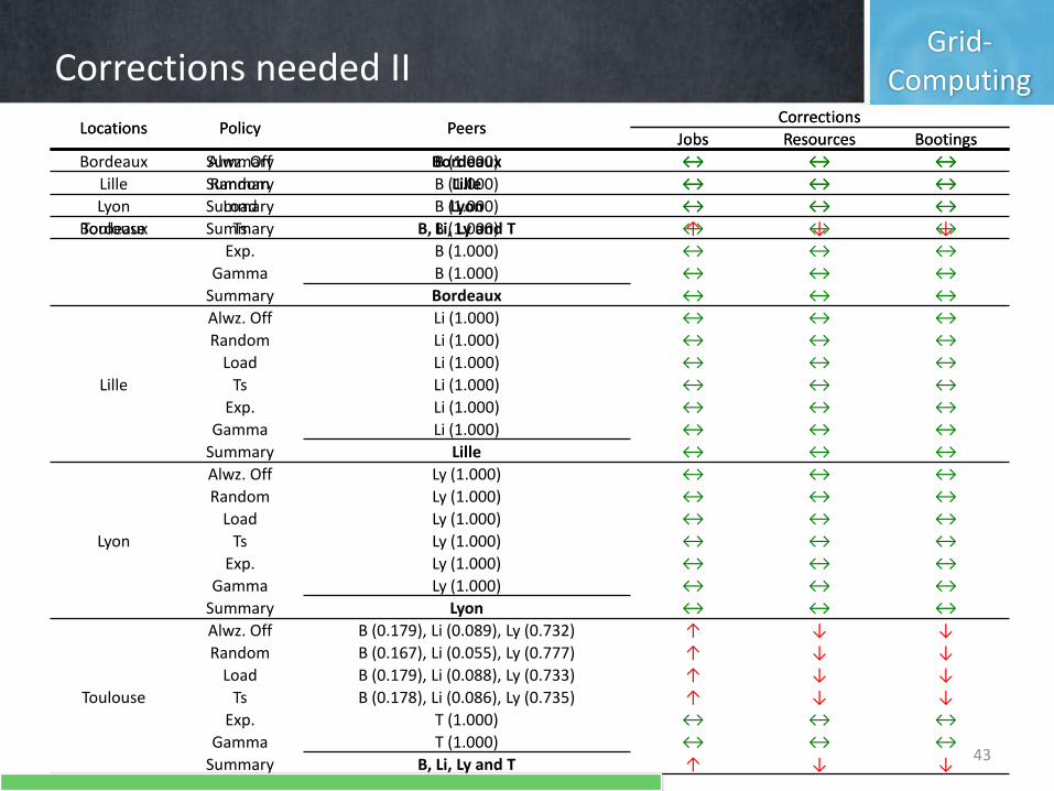
Grid-ComputingCorrections needed II

Locations Policy PeersCorrections

Jobs Resources Bootings

Bordeaux Summary Bordeaux ↔ ↔ ↔

Lille Summary Lille ↔ ↔ ↔

Lyon Summary Lyon ↔ ↔ ↔

Toulouse Summary B, Li, Ly and T ↑ ↓ ↓



Bordeaux

Alwz. Off B (1.000) ↔ ↔ ↔

Random B (1.000) ↔ ↔ ↔

Load B (1.000) ↔ ↔ ↔

Ts B (1.000) ↔ ↔ ↔

Exp. B (1.000) ↔ ↔ ↔

Gamma B (1.000) ↔ ↔ ↔

Summary Bordeaux ↔ ↔ ↔

Lille

Alwz. Off Li (1.000) ↔ ↔ ↔

Random Li (1.000) ↔ ↔ ↔

Load Li (1.000) ↔ ↔ ↔

Ts Li (1.000) ↔ ↔ ↔

Exp. Li (1.000) ↔ ↔ ↔

Gamma Li (1.000) ↔ ↔ ↔

Summary Lille ↔ ↔ ↔

Lyon

Alwz. Off Ly (1.000) ↔ ↔ ↔

Random Ly (1.000) ↔ ↔ ↔

Load Ly (1.000) ↔ ↔ ↔

Ts Ly (1.000) ↔ ↔ ↔

Exp. Ly (1.000) ↔ ↔ ↔

Gamma Ly (1.000) ↔ ↔ ↔

Summary Lyon ↔ ↔ ↔

Toulouse

Alwz. Off B (0.179), Li (0.089), Ly (0.732) ↑ ↓ ↓

Random B (0.167), Li (0.055), Ly (0.777) ↑ ↓ ↓

Load B (0.179), Li (0.088), Ly (0.733) ↑ ↓ ↓

Ts B (0.178), Li (0.086), Ly (0.735) ↑ ↓ ↓

Exp. T (1.000) ↔ ↔ ↔

Gamma T (1.000) ↔ ↔ ↔

Summary B, Li, Ly and T ↑ ↓ ↓43

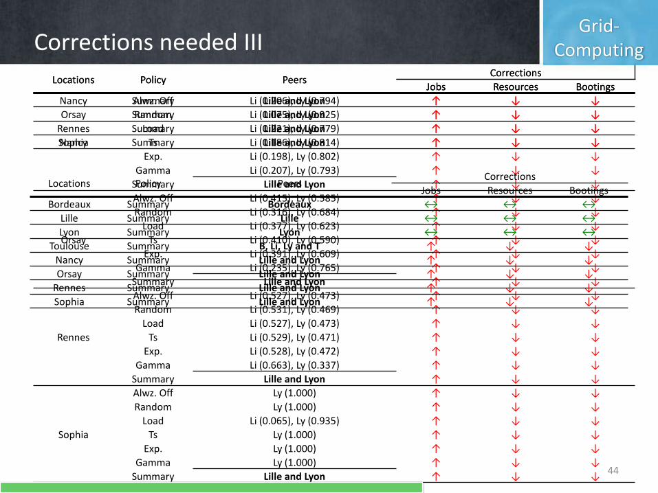
Grid-ComputingCorrections needed III

44



Nancy

Alwz. Off Li (0.206), Ly (0.794) ↑ ↓ ↓

Random Li (0.075), Ly (0.925) ↑ ↓ ↓

Load Li (0.221), Ly (0.779) ↑ ↓ ↓

Ts Li (0.186), Ly (0.814) ↑ ↓ ↓

Exp. Li (0.198), Ly (0.802) ↑ ↓ ↓

Gamma Li (0.207), Ly (0.793) ↑ ↓ ↓

Summary Lille and Lyon ↑ ↓ ↓

Orsay

Alwz. Off Li (0.415), Ly (0.585) ↑ ↓ ↓

Random Li (0.316), Ly (0.684) ↑ ↓ ↓

Load Li (0.377), Ly (0.623) ↑ ↓ ↓

Ts Li (0.410), Ly (0.590) ↑ ↓ ↓

Exp. Li (0.391), Ly (0.609) ↑ ↓ ↓

Gamma Li (0.235), Ly (0.765) ↑ ↓ ↓


Rennes

Alwz. Off Li (0.527), Ly (0.473) ↑ ↓ ↓

Random Li (0.531), Ly (0.469) ↑ ↓ ↓

Load Li (0.527), Ly (0.473) ↑ ↓ ↓

Ts Li (0.529), Ly (0.471) ↑ ↓ ↓

Exp. Li (0.528), Ly (0.472) ↑ ↓ ↓

Gamma Li (0.663), Ly (0.337) ↑ ↓ ↓


Sophia

Alwz. Off Ly (1.000) ↑ ↓ ↓

Random Ly (1.000) ↑ ↓ ↓

Load Li (0.065), Ly (0.935) ↑ ↓ ↓

Ts Ly (1.000) ↑ ↓ ↓

Exp. Ly (1.000) ↑ ↓ ↓

Gamma Ly (1.000) ↑ ↓ ↓




Nancy Summary Lille and Lyon ↑ ↓ ↓

Orsay Summary Lille and Lyon ↑ ↓ ↓

Rennes Summary Lille and Lyon ↑ ↓ ↓

Sophia Summary Lille and Lyon ↑ ↓ ↓



Bordeaux Summary Bordeaux ↔ ↔ ↔

Lille Summary Lille ↔ ↔ ↔

Lyon Summary Lyon ↔ ↔ ↔

Toulouse Summary B, Li, Ly and T ↑ ↓ ↓

Nancy Summary Lille and Lyon ↑ ↓ ↓

Orsay Summary Lille and Lyon ↑ ↓ ↓

Rennes Summary Lille and Lyon ↑ ↓ ↓

Sophia Summary Lille and Lyon ↑ ↓ ↓

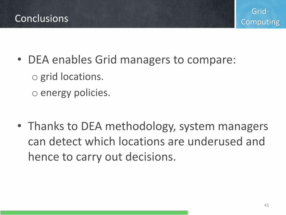
Grid-ComputingConclusions

45

• DEA enables Grid managers to compare:

o grid locations.

o energy policies.

• Thanks to DEA methodology, system managers can detect which locations are underused and hence to carry out decisions.

Grid-Computing

46

JCR 2.203, JCR-5 2.455Q1 in three categories:

Engineering, Electrical & Electronic (41/244)Operations Research & Management Science (5/77)Computer Science, Artificial Intelligence (22/111)

Lighting, Wireless Sensor Networks, User preferences

Smart environments Lighting adjustment,

User preferences

SmartEnvironmentsIntroduction

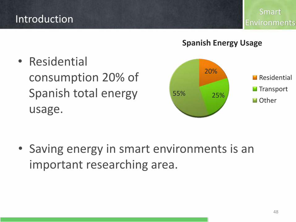
• Residential consumption 20% of Spanish total energy usage.

20%

25%55%

Spanish Energy Usage

Residential

Transport

Other

48

• Saving energy in smart environments is an important researching area.

SmartEnvironmentsIntroduction

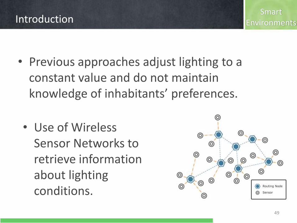
• Previous approaches adjust lighting to a constant value and do not maintain knowledge of inhabitants’ preferences.

• Use of Wireless Sensor Networks to retrieve information about lighting conditions.

49

SmartEnvironmentsMotivation

50

• Spanish technical building code establishes 400 lumens as the optimal quantity of light for a standard office.

• Measures may vary depending on:

o sensors location.

o type of lighting appliances.

o windows orientation, size, etc.

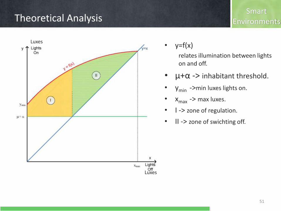
SmartEnvironmentsTheoretical Analysis

• y=f(x)

relates illumination between lights on and off.

• µ+α -> inhabitant threshold.

• ymin ->min luxes lights on.

• xmax -> max luxes.

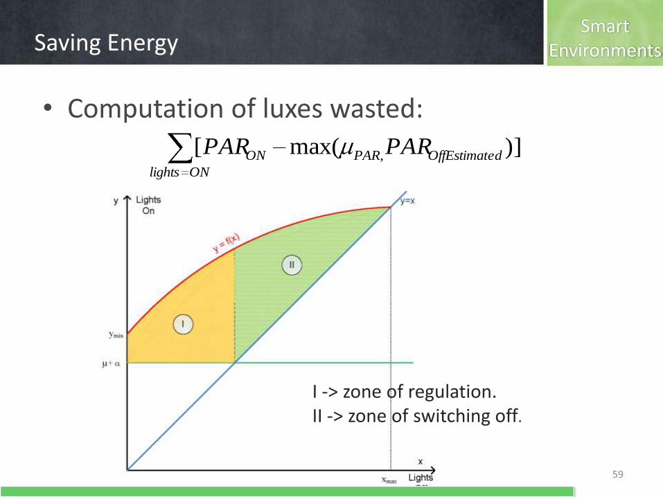
• I -> zone of regulation.

• II -> zone of swichting off.

51

Luxes

Luxes

SmartEnvironmentsExperimental Environment

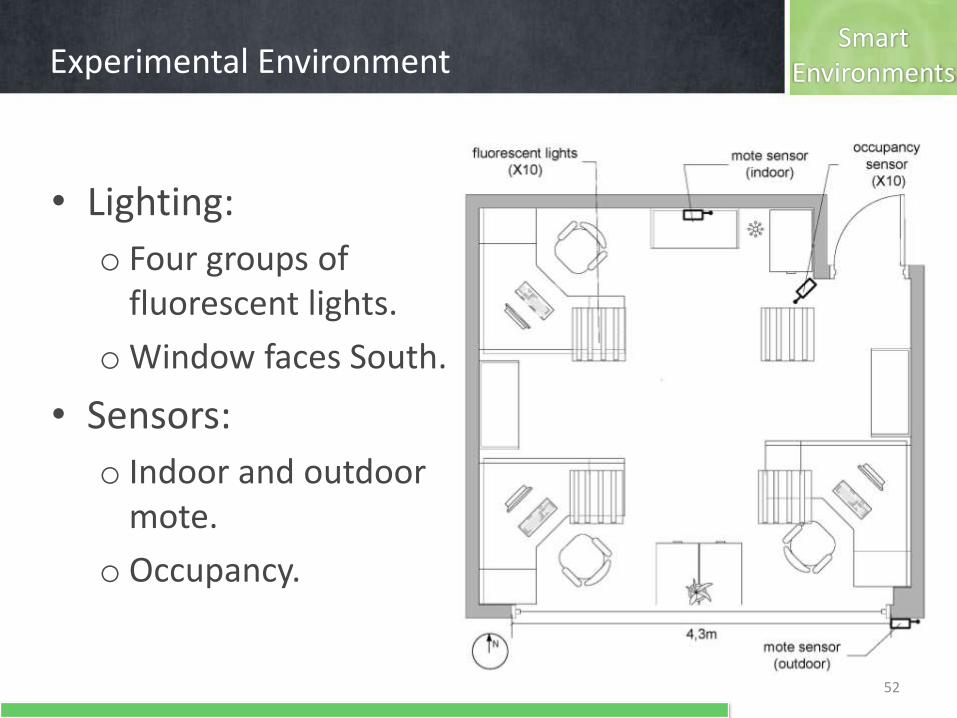
• Lighting:

o Four groups of fluorescent lights.

o Window faces South.

• Sensors:

o Indoor and outdoor mote.

o Occupancy.

52


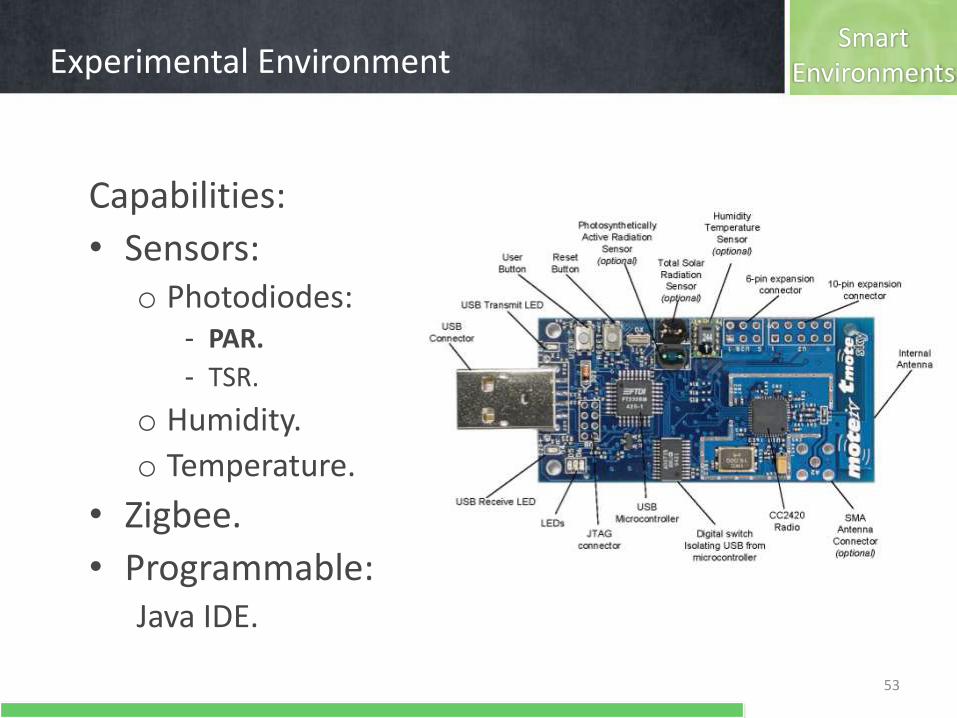
Capabilities:

• Sensors:o Photodiodes:

- PAR.

- TSR.

o Humidity.

o Temperature.

• Zigbee.

• Programmable:Java IDE.

53


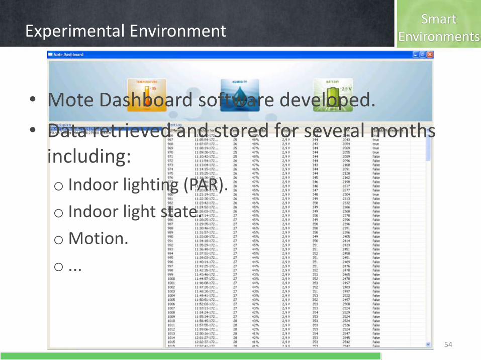
• Mote Dashboard software developed.

• Data retrieved and stored for several months including:

o Indoor lighting (PAR).

o Indoor light state.

o Motion.

o ...

54

SmartEnvironmentsUser Preference Threshold

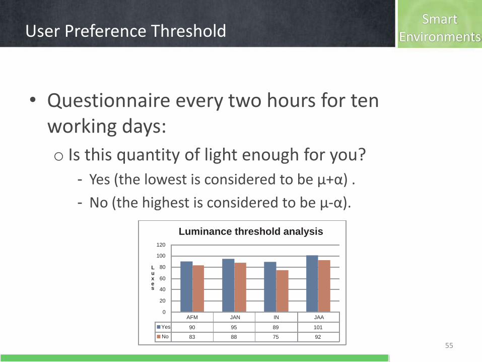
• Questionnaire every two hours for ten working days:

o Is this quantity of light enough for you?

- Yes (the lowest is considered to be μ+α) .

- No (the highest is considered to be μ-α).

AFM JAN IN JAA

Yes 90 95 89 101

No 83 88 75 92

0

20

40

60

80

100

120

s e x u L

Luminance threshold analysis

55

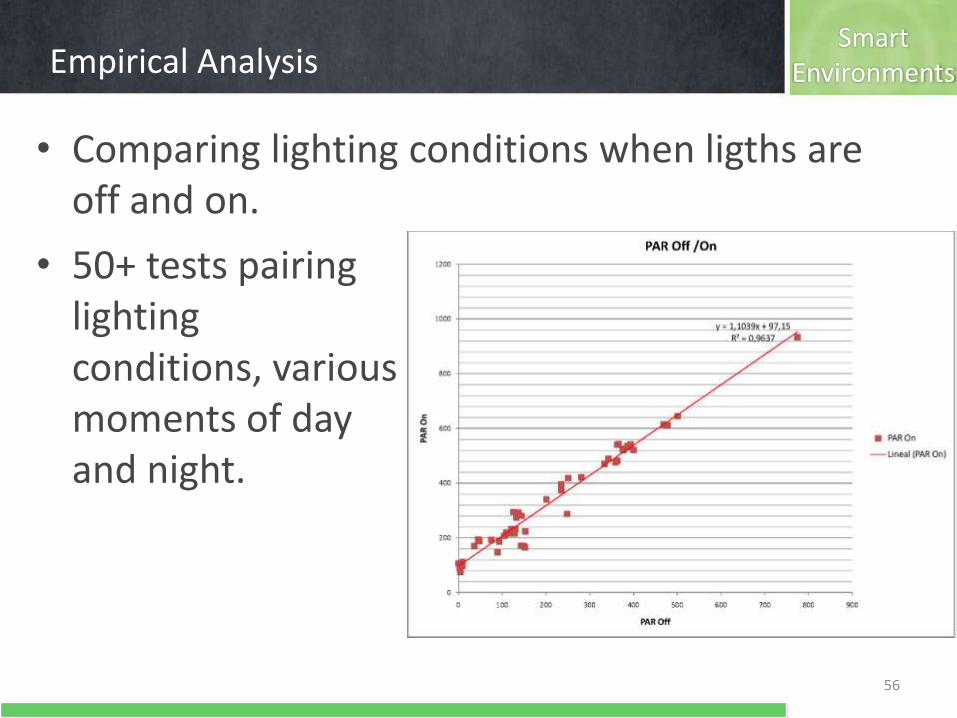
SmartEnvironmentsEmpirical Analysis

• Comparing lighting conditions when ligths are off and on.

• 50+ tests pairing lighting conditions, various moments of day and night.

56

SmartEnvironmentsEmpirical Analysis

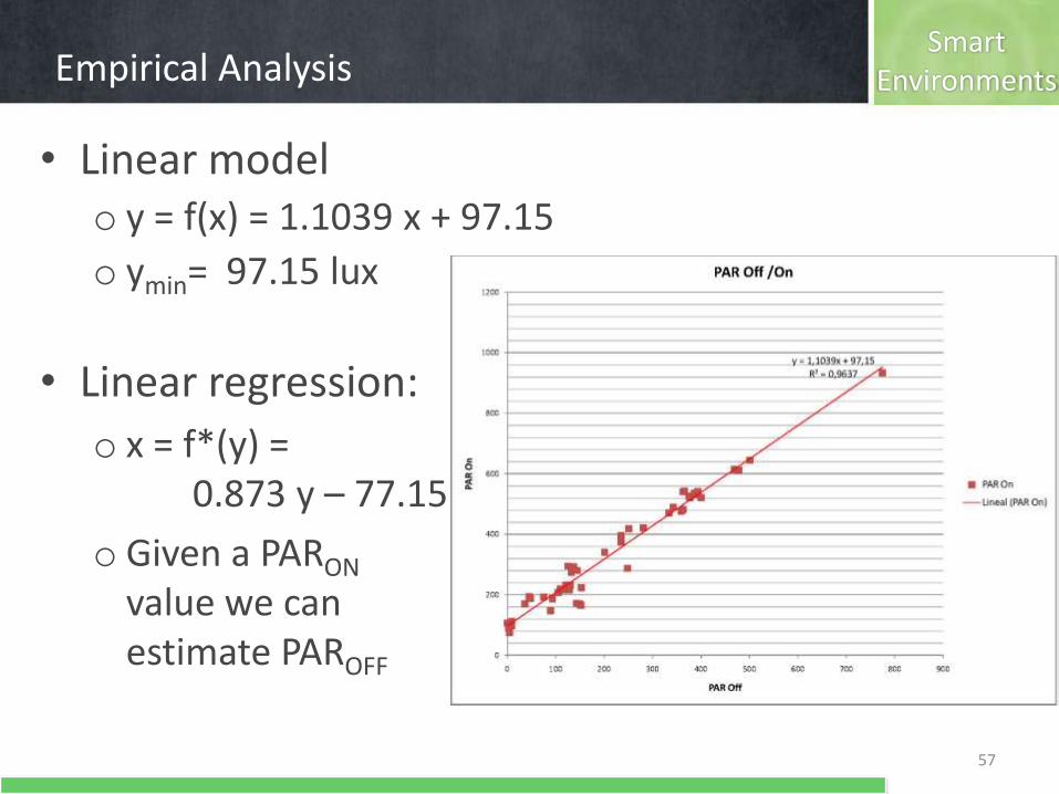
• Linear modelo y = f(x) = 1.1039 x + 97.15

o ymin= 97.15 lux

• Linear regression:

o x = f*(y) = 0.873 y – 77.15

o Given a PARON

value we can estimate PAROFF

57

SmartEnvironmentsSaving Energy

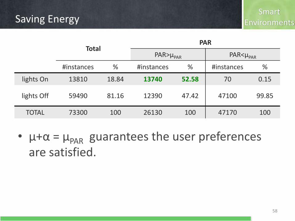
• μ+α = μPAR guarantees the user preferences are satisfied.

TotalPAR

PAR>µPAR PAR<µPAR

#instances % #instances % #instances %

lights On 13810 18.84 13740 52.58 70 0.15

lights Off 59490 81.16 12390 47.42 47100 99.85

TOTAL 73300 100 26130 100 47170 100

58


59

•

)(ONlights

edOffEstimatON PARPAR

)]max([ ,

ONlights

edOffEstimatPARON PARPAR

• Computation of luxes wasted:

I -> zone of regulation.II -> zone of switching off.


60

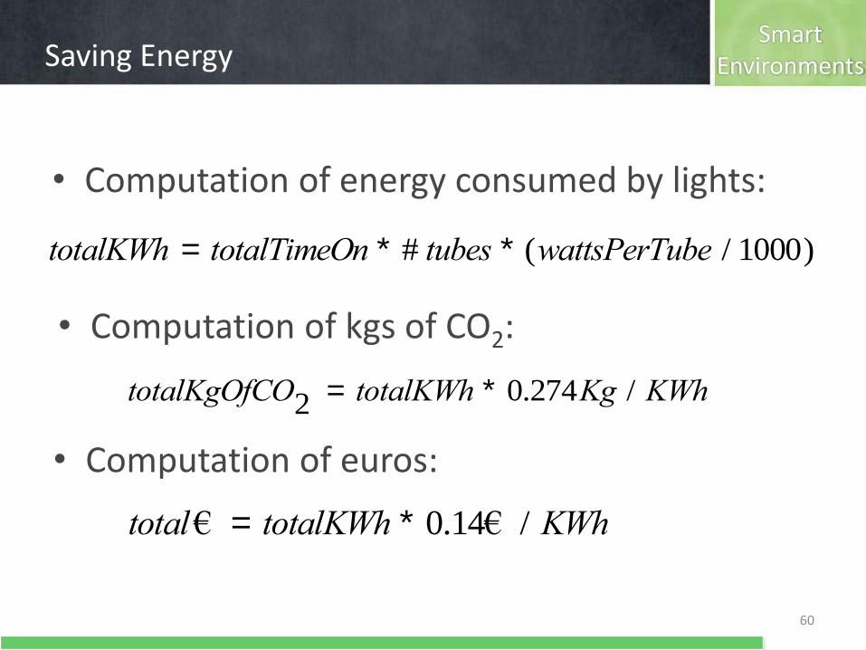
• Computation of energy consumed by lights:

totalKWh = totalTimeOn * # tubes * (wattsPerTube / 1000)

totalKgOfCO2 = totalKWh * 0.274Kg / KWh

total€ = totalKWh * 0.14€ / KWh

• Computation of kgs of CO2:

• Computation of euros:


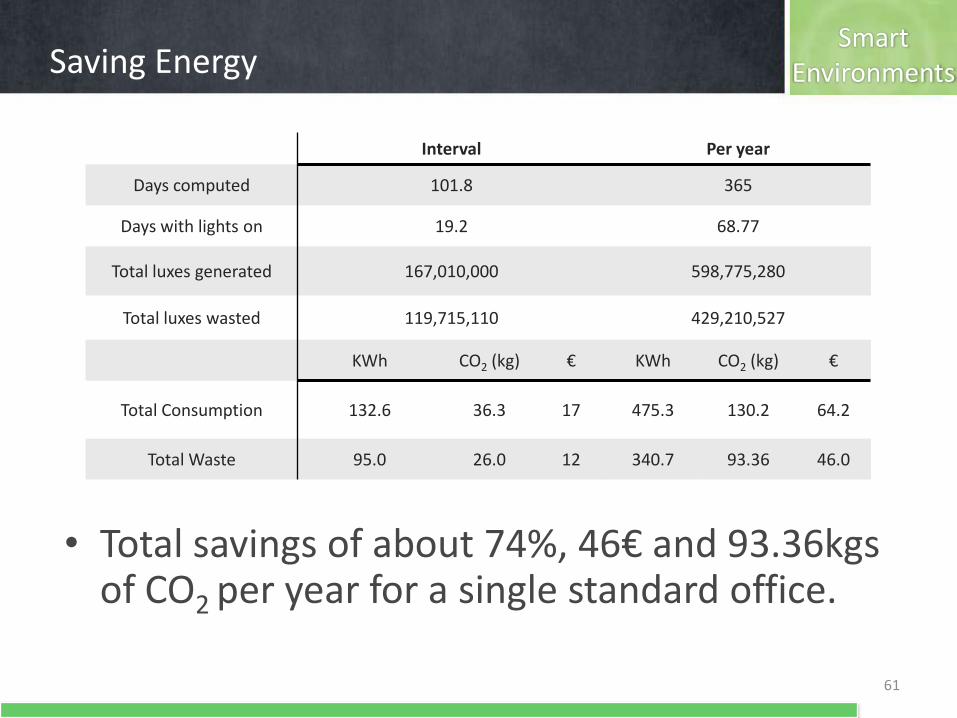
Interval Per year

Days computed 101.8 365

Days with lights on 19.2 68.77

Total luxes generated 167,010,000 598,775,280

Total luxes wasted 119,715,110 429,210,527

KWh CO2 (kg) € KWh CO2 (kg) €

Total Consumption 132.6 36.3 17 475.3 130.2 64.2

Total Waste 95.0 26.0 12 340.7 93.36 46.0

• Total savings of about 74%, 46€ and 93.36kgs of CO2 per year for a single standard office.

61

SmartEnvironments

62

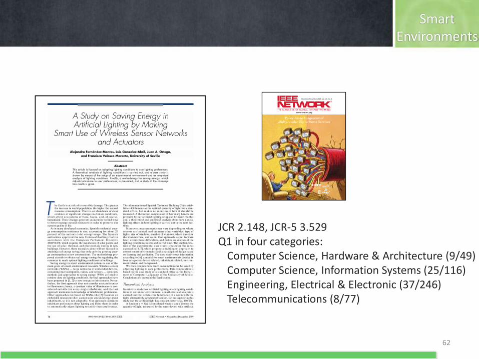
JCR 2.148, JCR-5 3.529Q1 in four categories:

Computer Science, Hardware & Architecture (9/49) Computer Science, Information Systems (25/116) Engineering, Electrical & Electronic (37/246) Telecommunications (8/77)

Final RemarksConclusions & Future Work,

Curriculum

Data center, Stress measurement, Curriculum

FinalRemarksConclusions

64

• Various energy saving policies have been designed and tested

– These energy policies can save up to 40% of energy on Grid-Computing infrastructures.

• DEA is a useful tool for comparing efficiency of locations and suggesting improvements.

– measures relative efficiency between locations, useful to take corrective decisions.

FinalRemarksConclusions

65

• Energy and economic costs savings can be carried out by means of cheap devices such as sensors and control appliances

• Energy policies applied to lighting conditions and based on user preferences can save up to 74% of energy.

FinalRemarksFuture work

66

• Grid-Computing:

o Adapting energy policies to take into account the variety of energy consumptions of resources.

o Adapting models to data centers issues.

o Development of new policies and combination of policies.

• Smart Environments:

o Collaboration with U. Reutlingen in order to extend Smart Environments model where biometric information is considered.

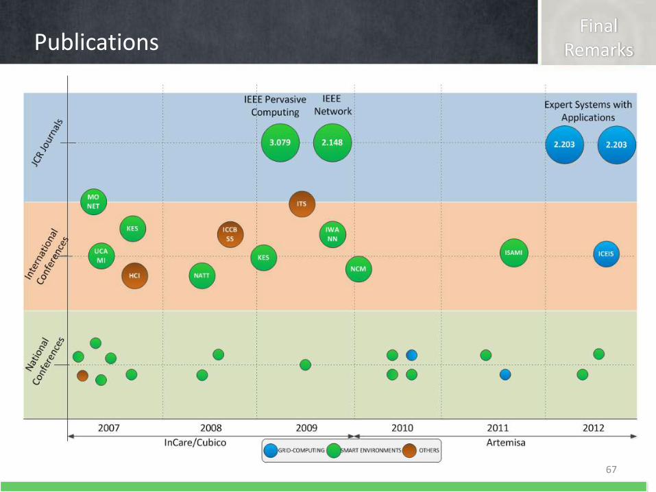
FinalRemarksPublications

67

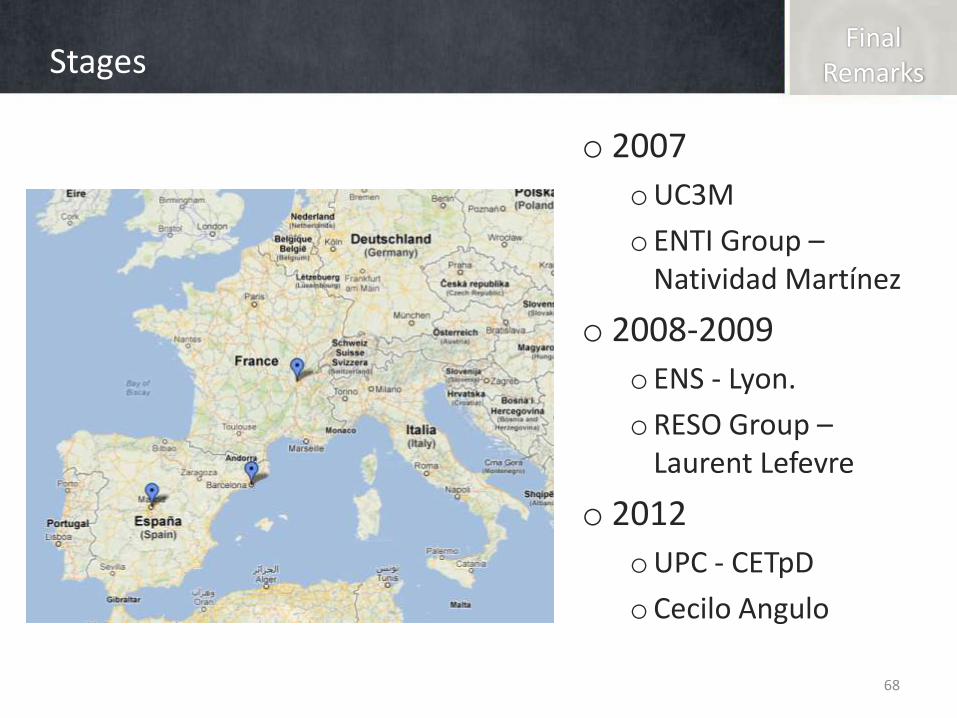
FinalRemarksStages

68

o 2007

oUC3M

o ENTI Group –Natividad Martínez

o 2008-2009

o ENS - Lyon.

oRESO Group –Laurent Lefevre

o 2012

oUPC - CETpD

oCecilo Angulo

Alejandro Fernández-Montes González

Advisors: Juan Antonio Ortega

Luis González Abril

Energy-Saving Policies in

Grid-Computing and

Smart Environments

Entertainment & Humor

Energy saving policies final