Response of Ocean Biogeochemistry and Isotopes to Different Iron Fluxes and Circulations

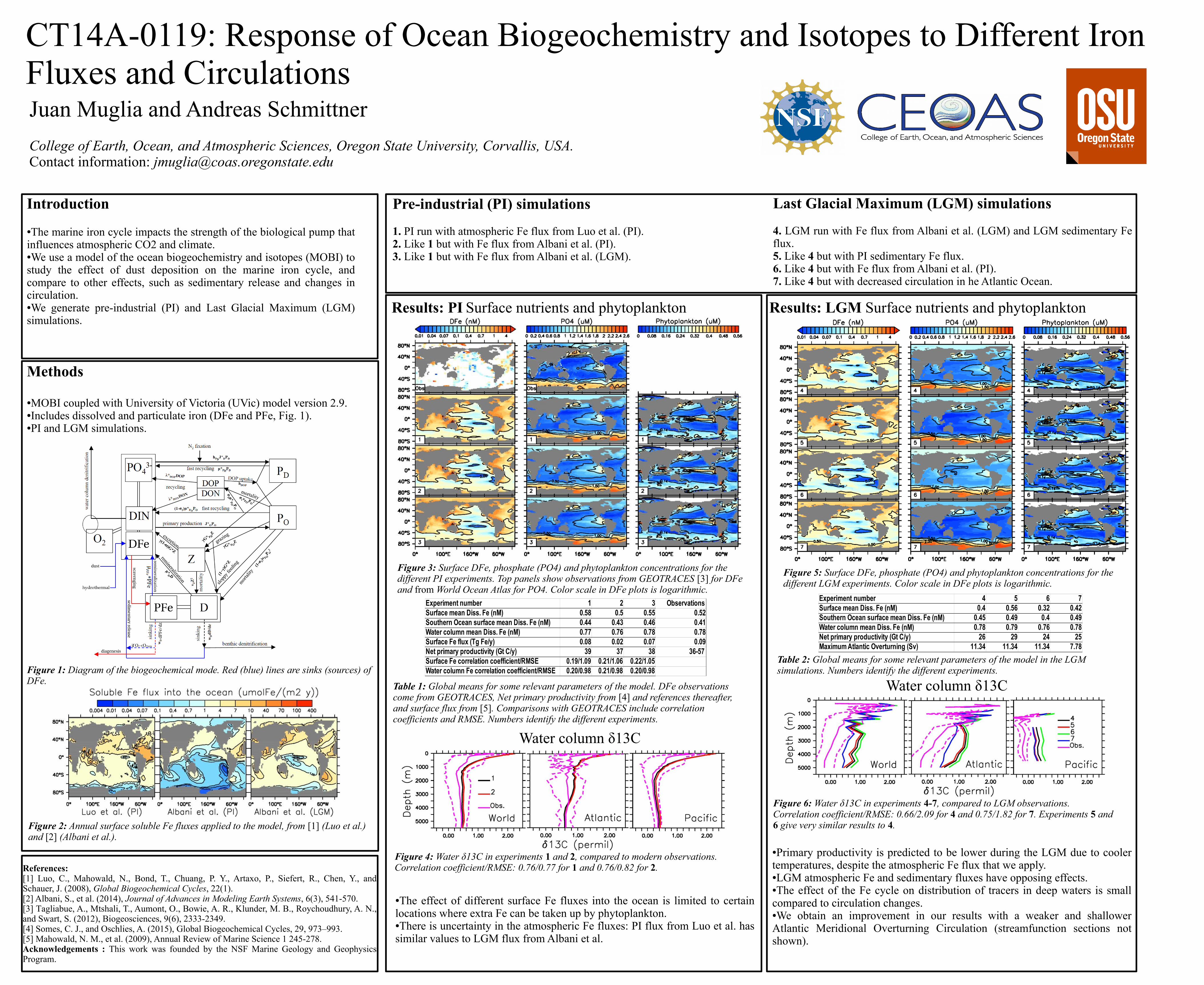
CT14A-0119: Response of Ocean Biogeochemistry and Isotopes to Different Iron Fluxes and Circulations

Juan Muglia and Andreas Schmittner College of Earth, Ocean, and Atmospheric Sciences, Oregon State University, Corvallis, USA.Contact information: [email protected]

Figure 1: Diagram of the biogeochemical mode. Red (blue) lines are sinks (sources) of DFe.

Methods

●MOBI coupled with University of Victoria (UVic) model version 2.9.●Includes dissolved and particulate iron (DFe and PFe, Fig. 1).●PI and LGM simulations.

References: [1] Luo, C., Mahowald, N., Bond, T., Chuang, P. Y., Artaxo, P., Siefert, R., Chen, Y., and Schauer, J. (2008), Global Biogeochemical Cycles, 22(1).[2] Albani, S., et al. (2014), Journal of Advances in Modeling Earth Systems, 6(3), 541-570.[3] Tagliabue, A., Mtshali, T., Aumont, O., Bowie, A. R., Klunder, M. B., Roychoudhury, A. N., and Swart, S. (2012), Biogeosciences, 9(6), 2333-2349.[4] Somes, C. J., and Oschlies, A. (2015), Global Biogeochemical Cycles, 29, 973–993.[5] Mahowald, N. M., et al. (2009), Annual Review of Marine Science 1 245-278.Acknowledgements : This work was founded by the NSF Marine Geology and Geophysics Program.

Introduction

●The marine iron cycle impacts the strength of the biological pump that influences atmospheric CO2 and climate. ●We use a model of the ocean biogeochemistry and isotopes (MOBI) to study the effect of dust deposition on the marine iron cycle, and compare to other effects, such as sedimentary release and changes in circulation. ●We generate pre-industrial (PI) and Last Glacial Maximum (LGM) simulations.

Figure 2: Annual surface soluble Fe fluxes applied to the model, from [1] (Luo et al.) and [2] (Albani et al.).

Results: PI Results: LGM

Experiment number 1 2 3 ObservationsSurface mean Diss. Fe (nM) 0.58 0.5 0.55 0.52Southern Ocean surface mean Diss. Fe (nM) 0.44 0.43 0.46 0.41Water column mean Diss. Fe (nM) 0.77 0.76 0.78 0.78Surface Fe flux (Tg Fe/y) 0.08 0.02 0.07 0.09Net primary productivity (Gt C/y) 39 37 38 36-57Surface Fe correlation coefficient/RMSE 0.19/1.09 0.21/1.06 0.22/1.05Water column Fe correlation coefficient/RMSE 0.20/0.98 0.21/0.98 0.20/0.98

Experiment number 4 5 6 7Surface mean Diss. Fe (nM) 0.4 0.56 0.32 0.42Southern Ocean surface mean Diss. Fe (nM) 0.45 0.49 0.4 0.49Water column mean Diss. Fe (nM) 0.78 0.79 0.76 0.78Net primary productivity (Gt C/y) 26 29 24 25Maximum Atlantic Overturning (Sv) 11.34 11.34 11.34 7.78

Figure 3: Surface DFe, phosphate (PO4) and phytoplankton concentrations for the different PI experiments. Top panels show observations from GEOTRACES [3] for DFe and from World Ocean Atlas for PO4. Color scale in DFe plots is logarithmic.

Last Glacial Maximum (LGM) simulations

4. LGM run with Fe flux from Albani et al. (LGM) and LGM sedimentary Fe flux. 5. Like 4 but with PI sedimentary Fe flux. 6. Like 4 but with Fe flux from Albani et al. (PI).7. Like 4 but with decreased circulation in he Atlantic Ocean.

Pre-industrial (PI) simulations 1. PI run with atmospheric Fe flux from Luo et al. (PI).2. Like 1 but with Fe flux from Albani et al. (PI).3. Like 1 but with Fe flux from Albani et al. (LGM).

Surface nutrients and phytoplankton Surface nutrients and phytoplankton

Figure 5: Surface DFe, phosphate (PO4) and phytoplankton concentrations for the different LGM experiments. Color scale in DFe plots is logarithmic.

Table 1: Global means for some relevant parameters of the model. DFe observations come from GEOTRACES, Net primary productivity from [4] and references thereafter, and surface flux from [5]. Comparisons with GEOTRACES include correlation coefficients and RMSE. Numbers identify the different experiments.

Table 2: Global means for some relevant parameters of the model in the LGM simulations. Numbers identify the different experiments.

Water column δ13C

Water column δ13C

Figure 4: Water δ13C in experiments 1 and 2, compared to modern observations. Correlation coefficient/RMSE: 0.76/0.77 for 1 and 0.76/0.82 for 2.

Figure 6: Water δ13C in experiments 4-7, compared to LGM observations. Correlation coefficient/RMSE: 0.66/2.09 for 4 and 0.75/1.82 for 7. Experiments 5 and 6 give very similar results to 4.

●The effect of different surface Fe fluxes into the ocean is limited to certain locations where extra Fe can be taken up by phytoplankton.●There is uncertainty in the atmospheric Fe fluxes: PI flux from Luo et al. has similar values to LGM flux from Albani et al.

●Primary productivity is predicted to be lower during the LGM due to cooler temperatures, despite the atmospheric Fe flux that we apply. ●LGM atmospheric Fe and sedimentary fluxes have opposing effects. ●The effect of the Fe cycle on distribution of tracers in deep waters is small compared to circulation changes.●We obtain an improvement in our results with a weaker and shallower Atlantic Meridional Overturning Circulation (streamfunction sections not shown).