Embed Size (px)
Citation preview

林隆慧
卡方检验

Chi-square (x) goodness of fit
Chi-square goodness of fit is widely used to infer whether the population from which a sample of nominal data came conforms to a certain theoretical distribution.
e.g., a plant geneticist may raise 100 progeny from a cross that is hypothesized to result a 3:1 phenotypic ratio of pink-flowered to white-flowered. Perhaps a ratio of 84 pink: 16 white is observed, although out of this total of 100 roses, the geneticist’s hypothesis would predict a ratio of 75 pink: 25 white. The question to be answered, then, is whether the observed frequencies deviate significantly from the frequencies expected if the hypothesis were true

Chi-square (x) goodness of fit
The following calculation of a statistic called chi-square is used as a measure of how far a sample distribution deviate from a theoretical distribution
Here, Oi is the frequency, or number of counts, observed in class i, Ei is the frequency expected in class i if the null hypothesis is true, and the summation is performed over all k categories of data.
Larger disagreement between observed and expected frequencies will results in a larger x2 value. Thus, this type of calculation is referred to as a measure of goodness of fit. A calculated x2 value can be as small as zero, in the case of perfect fit.

Chi-square goodness of fit for two categories
Calculation of chi-square goodness of fit for k = 2 (e.g., data consisting of 100 flower colors to a hypothesized color ratio of 3: 1)
Categories (flower color)
H0: The sample data came from a population having a 3: 1 ratio of pink to white flowersHA: The sample data came from a population not having a 3: 1 flower color ratio
Pink White
Oi
(Ei )
84 16
(75) (25)
degree of freedom = = k – 1 = 2 – 1 = 1
= (84 – 75)2/75 + (16 – 25)2/25 = 4.320
0.025 < P < 0.05. Therefore, reject H0 and accept HA
n
100

Statistical errors in hypothesis testing
A probability of 5% or less is commonly used as the criterion for rejection of H0. The probability used as the criterion for rejection is termed the significance level, denoted by , and the value of the test statistic corresponding to this probability is the critical value (临界值 ) of the statistic.
It is very important to realize that a true null hypothesis occasionally will be rejected, which of course means that we have committed an error. This error will be committed with a frequency of . That is, if H0 is in fact a true statement about a statistical population, it will be concluded erroneously to be false 5% of the time.

Two types of statistical errors
Type I error: The rejection of a null hypothesis when it is in fact a true statement is a Type I error (also called error, or an error of the first kind). (弃真 )
Type II error: On the other hand, if H0 is in fact false, our test may occasionally not detected this fact, and we shall have reached an erroneous conclusion by not rejecting H0. This error, of not rejecting the null hypothesis when it is in fact false, is a Type II error (also called error, or an error of the second kind).(纳伪)
If H0 is true If H0 is false
No error Type I error
No error Type II error
If H0 is rejected
If H0 is not rejected1-
1-

Chi-square goodness of fit for more than two categories
Calculation of chi-square goodness of fit for k = 4
Categories (flower color)
H0: The sample from a population having a 9: 3: 3: 1 color pattern of flowersHA: The sample from a population not having a 9: 3: 3: 1 color pattern of flowers
Red rayed Red margined
Oi
(Ei )
152 39
(140.6)
= k – 1 = 4 – 1 = 3
= 8.956
0.025 < P < 0.05. Therefore, reject H0 and accept HA
Blizzard Rayed
53 6
n
250
(46.9) (46.9) (15.6)
Red rayed
Red margined
BlizzardRayed

Chi-square correction for continuity
Chi-square values obtained from actual data belonging to discrete or discontinuous distribution. However, the theoretical x2 distribution is a continuous distribution. x2
values calculated obtained from discrete data ( = 1 in particular) are often overestimated and may therefore cause us to commit the Type I error with a probability greater than the stated .
The Yates correction (see below) should routinely be used when = 1

The log-likelihood ratio (G-test)
The x2 test is the traditional method for tests of GOF. The G-test is an alternative to the x2 test for analyzing frequencies. The two methods are interchangeable. The G-test is increasingly used because: it is easier to calculate; mathematicians believe it has theoretical advantages in advanced applications
G = 2 O ln (O/E) (ln = natural logarithm)
The G-test statistic (G) uses the same tables as the x2 test. The G-test is based on the principle that the ratios of two probabilities can be used as a test statistic to measure the degree of agreement between sampled and expected frequencies. Williams (1976) recommends G be used in preference to x2 whenever any
> expected frequency
The two methods often yield the same conclusions; when they do not, many statiscians prefer G test and therefore recommend its routine use

G-test for more than two categories
Categories (flower color)
H0: The sample from a population having a 9: 3: 3: 1 color pattern of flowersHA: The sample from a population not having a 9: 3: 3: 1 color pattern of flowers
Red rayed Red margined
Oi
(Ei )
152 39
(140.6)
= k – 1 = 4 – 1 = 3
0.001 < P < 0.025. Therefore, reject H0 and accept HA
Blizzard Rayed
53 6
n
250
(46.9) (46.9) (15.6)
Red rayed
Red margined
BlizzardRayed G = 2 O ln (O/E) = 10.807

2×2 联表的独立性检验

2×2 联表的独立性检验

2×2 联表的独立性检验

2×2 联表的独立性检验

2×2 联表的独立性检验

R×C 列联表的独立性检验
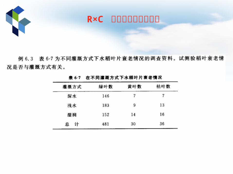
R×C 列联表的独立性检验

R×C 列联表的独立性检验Fisher’s Exact Test

R×C 列联表的独立性检验Fisher’s Exact Test
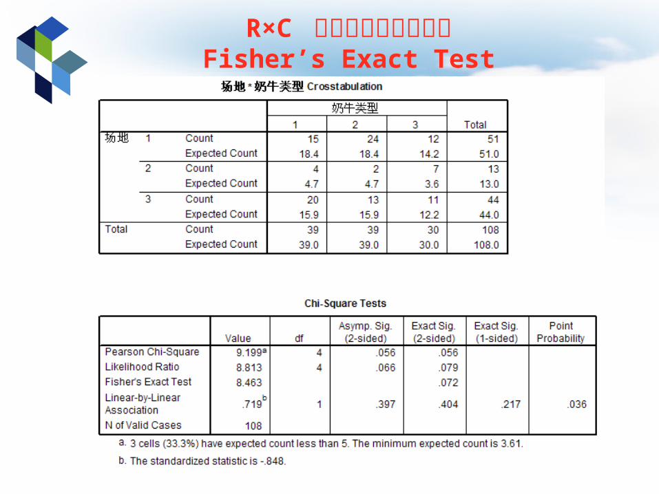
R×C 列联表的独立性检验Fisher’s Exact Test

配对卡方检验
把每一份样本平分为两份,分别用两种检测方法进行检测,比较两种方法的结果(两类计数资料)是否具有一致性或两种方法在哪些地方不一致
分别采用两种方法对同一批动、植物进行检查,比较此两种方法的结果是否有本质不同

配对卡方检验

配对卡方检验

配对卡方检验