以每年參觀 Lake Keepit 的人數為例

數 98 級乙班林柏佐

494402345

Variable

Dist=Distance Inc=Family Income Size=Family Members Y=Numbers of Vistors

pair

Residuals Plot-SLR

Box-Cox

Transformation

fm1<-lm(log(Y+1)~Dist+Inc+Size)在做轉換時，要注意各係數都必須是正數，因為 Y 有 0 ，所以我讓其加 1 ，來做 regression

Residuals Plot-Transformation

Select Model

fm2<-lm(log(Y+1)~Dist+Size) Coefficients: Estimate Std. Error t value Pr(>|t|) (Intercept) 1.613546 0.104927 15.378 < 2e-16 ***Dist -0.014158 0.001071 -13.218 < 2e-16 ***Size 0.084795 0.023403 3.623 0.000353 ***---Signif. codes: 0 ‘***’ 0.001 ‘**’ 0.01 ‘*’ 0.05 ‘.’ 0.1 ‘ ’ 1 Residual standard error: 0.5169 on 247 degrees of freedomMultiple R-squared: 0.4295, Adjusted R-squared: 0.4249 F-statistic: 92.99 on 2 and 247 DF, p-value: < 2.2e-16

Residuals Plot-Select Model

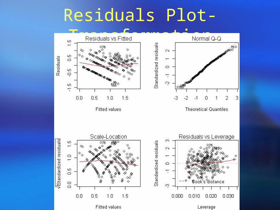
Variance Stable

Call:lm(formula = sqrt(Y) ~ Dist + Inc + Size)Residuals: Min 1Q Median 3Q Max -1.6186 -0.4273 0.0727 0.4570 1.6070 Coefficients: Estimate Std. Error t value Pr(>|t|) (Intercept) 1.884998 0.184333 10.226 < 2e-16 ***Dist -0.017528 0.001348 -13.000 < 2e-16 ***Inc 0.024612 0.018196 1.353 0.17742 Size 0.104933 0.029553 3.551 0.00046 ***---Signif. codes: 0 ‘***’ 0.001 ‘**’ 0.01 ‘*’ 0.05 ‘.’ 0.1 ‘ ’ 1 Residual standard error: 0.6507 on 246 degrees of freedomMultiple R-squared: 0.424, Adjusted R-squared: 0.417 F-statistic: 60.36 on 3 and 246 DF, p-value: < 2.2e-16

Residuals Plot-Variance Stable

WLS

lm(formula = sqrt(Y) ~ Dist + Inc + Size, weights = wi)Residuals: Min 1Q Median 3Q Max -3.1818 -0.8134 0.1118 0.9051 3.2484 Coefficients: Estimate Std. Error t value Pr(>|t|) (Intercept) 1.874293 0.181835 10.308 < 2e-16 ***Dist -0.018063 0.001328 -13.599 < 2e-16 ***Inc 0.027104 0.017669 1.534 0.126323# 收入太低決定將其拿掉Size 0.113891 0.029023 3.924 0.000113 ***---Signif. codes: 0 ‘***’ 0.001 ‘**’ 0.01 ‘*’ 0.05 ‘.’ 0.1 ‘ ’ 1 Residual standard error: 1.233 on 246 degrees of freedomMultiple R-squared: 0.4511, Adjusted R-squared: 0.4444 F-statistic: 67.38 on 3 and 246 DF, p-value: < 2.2e-16

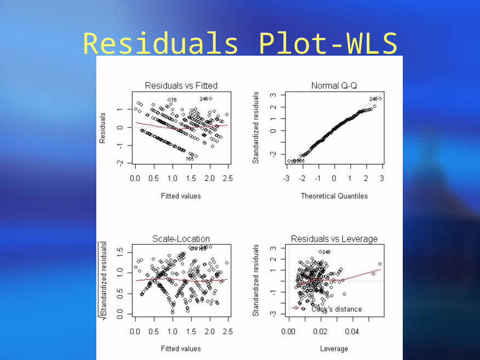
Residuals Plot-WLS

WLS+Model Selection

Call:lm(formula = sqrt(Y) ~ Dist + Size, weights = wi)Residuals: Min 1Q Median 3Q Max -3.2532 -0.8942 0.1028 0.9767 3.0845 Coefficients: Estimate Std. Error t value Pr(>|t|) (Intercept) 2.077797 0.124694 16.663 < 2e-16 ***Dist -0.018099 0.001332 -13.590 < 2e-16 ***Size 0.109893 0.028985 3.791 0.000188 ***---Signif. codes: 0 ‘***’ 0.001 ‘**’ 0.01 ‘*’ 0.05 ‘.’ 0.1 ‘ ’ 1 Residual standard error: 1.236 on 247 degrees of freedomMultiple R-squared: 0.4458, Adjusted R-squared: 0.4413 F-statistic: 99.34 on 2 and 247 DF, p-value: < 2.2e-16

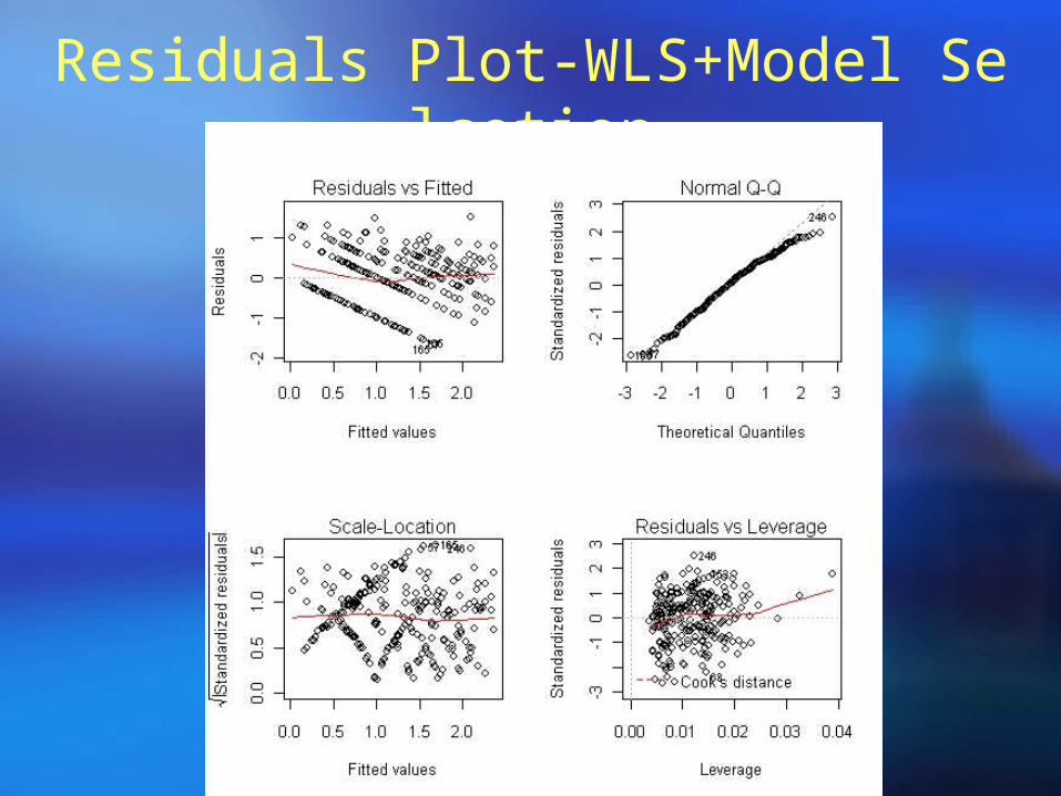
Residuals Plot-WLS+Model Selcetion

結論最後我選擇 這個 model, 但是其實還是有很多要改進，它的 R-squared 太低，解釋力不夠。或許利用generalized least square 可以解決這個問題。

2.077797 0.018099Dist 0.109893SizeY

The End

Thanks for your attention.