الفصل الدراسى السابع S-7 هندسة ميكروموجية Microwave Engineering 1

السابع الدراسى -Sالفصل7

ميكروموجية هندسة

Microwave Engineering

1

2

3

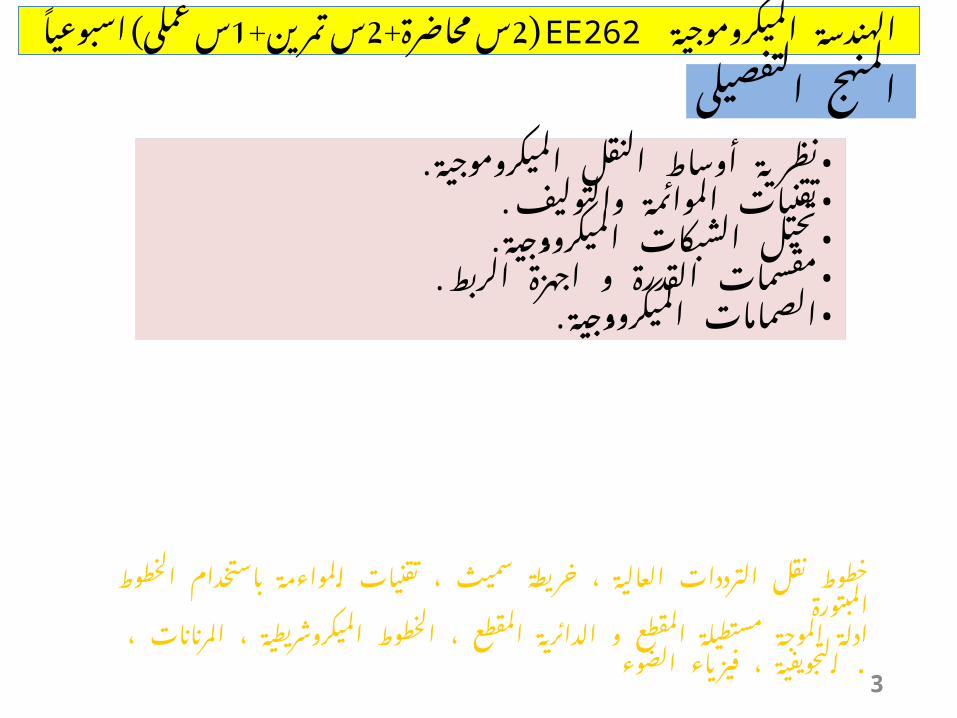
الميكروموجية +EE262( 2 الهندسة محاضرة +2س تمرين س 1س )! اسبوعيا عملى

الميكروموجية نظرية • النقل .أوساطالموائمة • والتوليف.تقنياتالميكرو • الشبكات ية.جومتحيل•. الربط اجهزة و القدرة مقسماتالميكرو • ية.جومالصمامات

المنهج التفصيلى

المواءمة تقنيات ، سميث خريطة ، العالية الترددات نقل خطوطالمبتورة الخطوط باستخدام

الخطوط ، ، المقطع الدائرية و المقطع مستطيلة الموجة ادلةالضوء فيزياء ، التجويفية المرنانات ، . الميكروشريطية

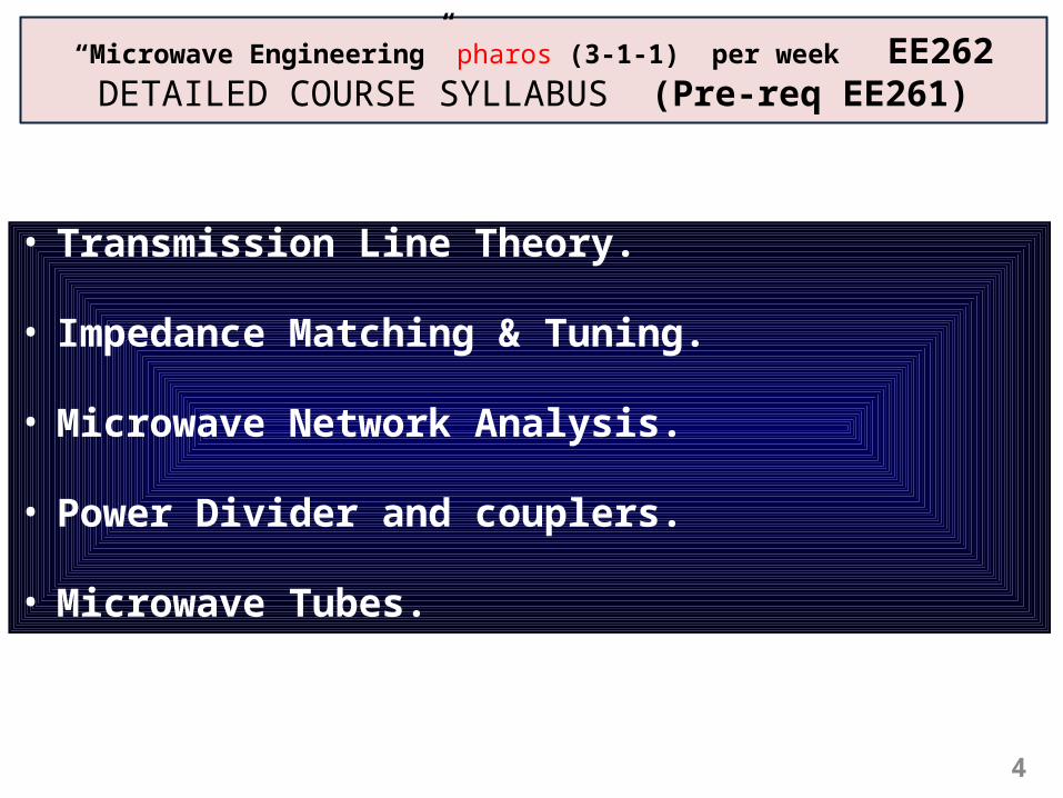
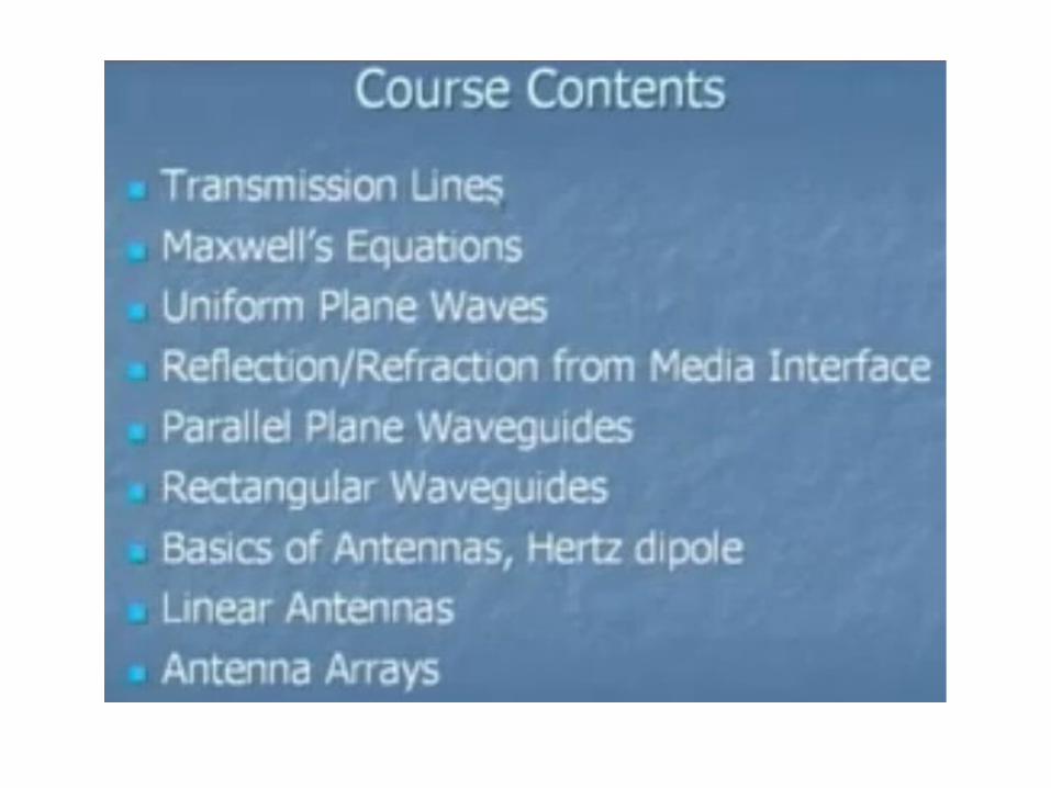
• Transmission Line Theory. • Impedance Matching & Tuning. • Microwave Network Analysis.

• Power Divider and couplers.

• Microwave Tubes.

4

“Microwave Engineering” pharos (3-1-1) per week EE262DETAILED COURSE SYLLABUS (Pre-req EE261)

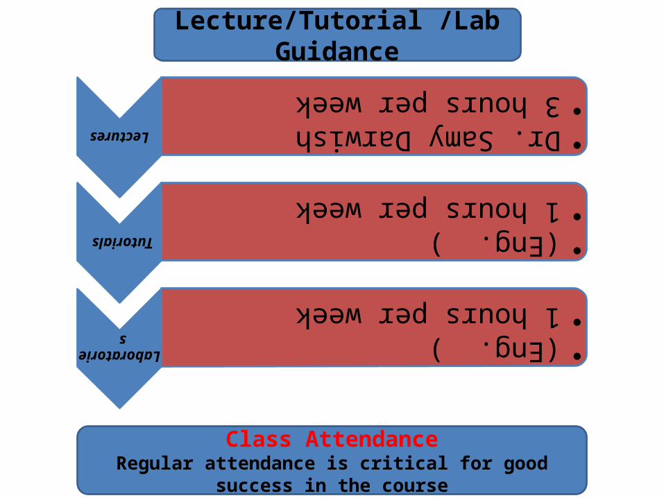
Lectures

•Dr. Samy Darwish

•3 hours per week

Tutorials

•(Eng. )

•1 hours per week

Laboratories

•(Eng. )

•1 hours per week

Lecture/Tutorial /Lab Guidance

Class AttendanceRegular attendance is critical for good success in the course

Evaluation methods i) Evaluation of class work including: -Drop Quizzes:10%. -Home work assignment & short reports and presentation: 15%.

ii) Mid term written exam @ 8th week: 25%.

v) Final examination: 50%.

Assessment Instruments ii) Short reports and presentation. iii) Quizzes.

Course Assessment

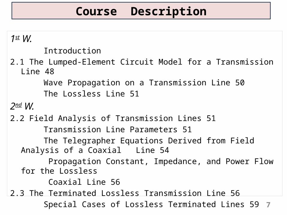
1st W. Introduction2.1 The Lumped-Element Circuit Model for a Transmission Line 48 Wave Propagation on a Transmission Line 50 The Lossless Line 51

2nd W.2.2 Field Analysis of Transmission Lines 51 Transmission Line Parameters 51 The Telegrapher Equations Derived from Field Analysis of a Coaxial Line 54 Propagation Constant, Impedance, and Power Flow for the Lossless Coaxial Line 562.3 The Terminated Lossless Transmission Line 56 Special Cases of Lossless Terminated Lines 59

Course Description

7

3rd W. 2.4 The Smith Chart 63 The Combined Impedance–Admittance Smith Chart 67 The Slotted Line 68

4th W.2.5 The Quarter-Wave Transformer 72The Impedance Viewpoint 72 The Multiple-Reflection Viewpoint 742.6 Generator and Load Mismatches 76Load Matched to Line 77 Generator Matched to Loaded Line 77Conjugate Matching 772.7 Lossy Transmission Lines 78The Low-Loss Line 79 The Distortionless Line 80The Terminated Lossy Line 81The Perturbation Method for Calculating Attenuation 82The Wheeler Incremental Inductance Rule 83

Course Description cont…

8

5th W. Impedance Matching & Tuning 2285.1 Matching with Lumped Elements (LNetworks) 229Analytic Solutions 230 Smith Chart Solutions 2315.2 Single-Stub Tuning 234Shunt Stubs 235 Series Stubs 2385.3 Double-Stub Tuning 241Smith Chart Solution 242 Analytic Solution 2455.4 The Quarter-Wave Transformer 246


9

6th W. Microwave Network Analysis. 1654.1 Impedance and Equivalent Voltages and Currents 166Equivalent Voltages and Currents 166 The Concept of Impedance 170Even and Odd Properties ofZ(ω)and(ω) 1734.2 Impedance and Admittance Matrices 174Reciprocal Networks 175 Lossless Networks 177

7th W. Microwave Network Analysis.4.3 The Scattering Matrix 178Reciprocal Networks and Lossless Networks 181A Shift in Reference Planes 184Power Waves and Generalized Scattering Parameters 1854.4 The Transmission(ABCD)Matrix 188Relation to Impedance Matrix 191Equivalent Circuits for Two-Port Networks 191


10

8th W. Microwave Network Analysis.

4.5 Signal Flow Graphs 194Decomposition of Signal Flow Graphs 195Application to Thru-Reflect-Line Network Analyzer Calibration 1974.6 Discontinuities and Modal Analysis 203Modal Analysis of an H-Plane Step in Rectangular Waveguide 203


11

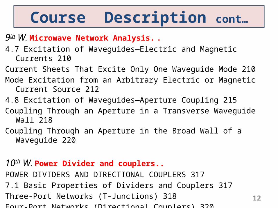
9th W. Microwave Network Analysis. .4.7 Excitation of Waveguides—Electric and Magnetic Currents 210Current Sheets That Excite Only One Waveguide Mode 210Mode Excitation from an Arbitrary Electric or Magnetic Current Source 2124.8 Excitation of Waveguides—Aperture Coupling 215Coupling Through an Aperture in a Transverse Waveguide Wall 218Coupling Through an Aperture in the Broad Wall of a Waveguide 220

10th W. Power Divider and couplers..POWER DIVIDERS AND DIRECTIONAL COUPLERS 3177.1 Basic Properties of Dividers and Couplers 317Three-Port Networks (T-Junctions) 318Four-Port Networks (Directional Couplers) 3207.2 The T-Junction Power Divider 324Lossless Divider 324 Resistive Divider 326


12

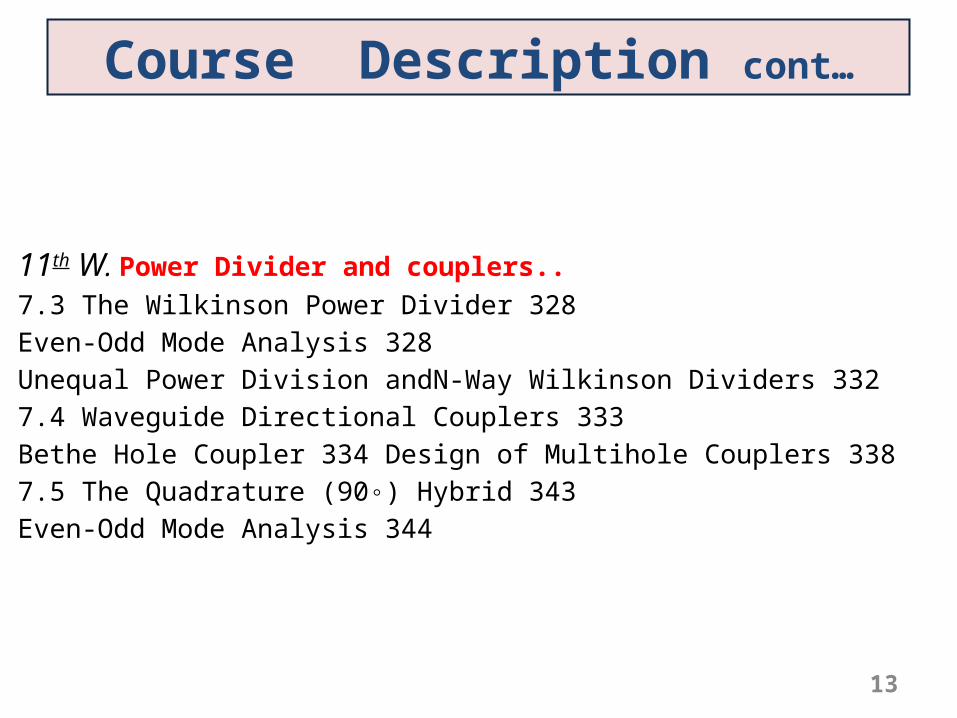
11th W. Power Divider and couplers..7.3 The Wilkinson Power Divider 328Even-Odd Mode Analysis 328Unequal Power Division andN-Way Wilkinson Dividers 3327.4 Waveguide Directional Couplers 333Bethe Hole Coupler 334 Design of Multihole Couplers 3387.5 The Quadrature (90◦) Hybrid 343Even-Odd Mode Analysis 344


13


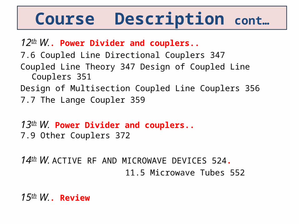
12th W.. Power Divider and couplers..7.6 Coupled Line Directional Couplers 347Coupled Line Theory 347 Design of Coupled Line Couplers 351Design of Multisection Coupled Line Couplers 3567.7 The Lange Coupler 359

13th W. Power Divider and couplers.. 7.9 Other Couplers 372

14th W. ACTIVE RF AND MICROWAVE DEVICES 524. 11.5 Microwave Tubes 552

15th W.. Review

األسبوع األول

15

introduction

Introduction to

Microwave Engineering

What happened if the frequency increase?What is the relation between frequency of electro magnetic waves and dimension of electric elements?

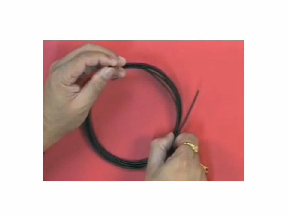
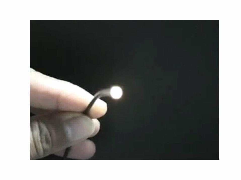
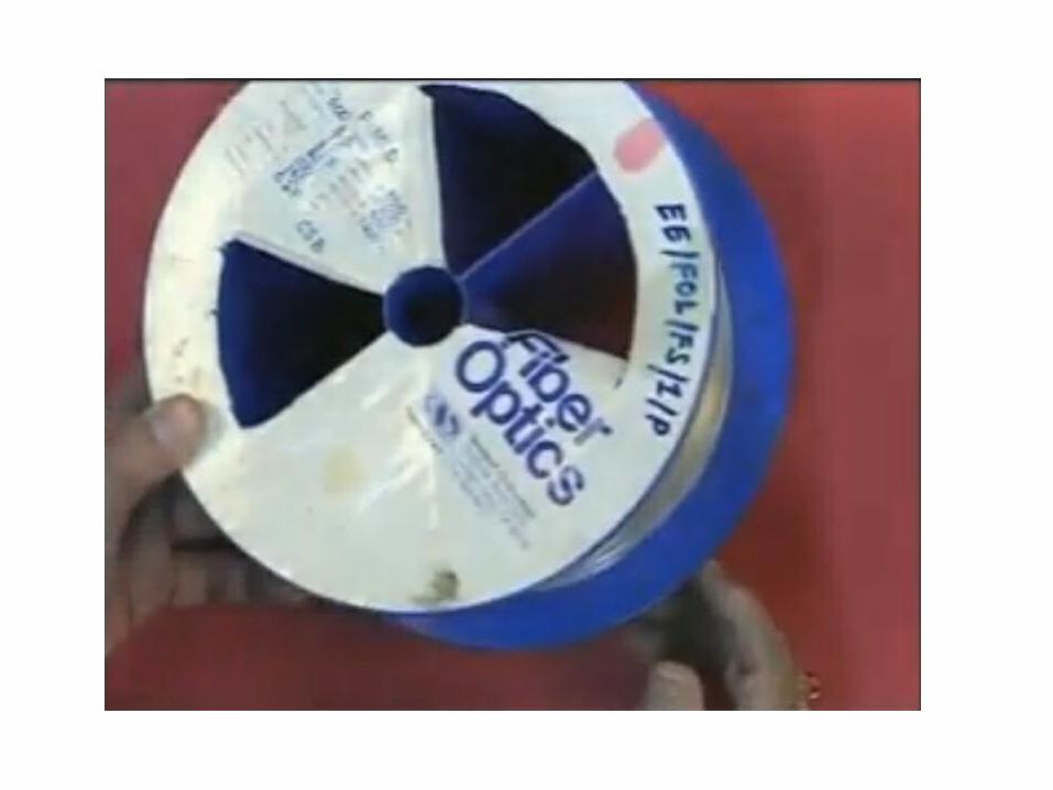
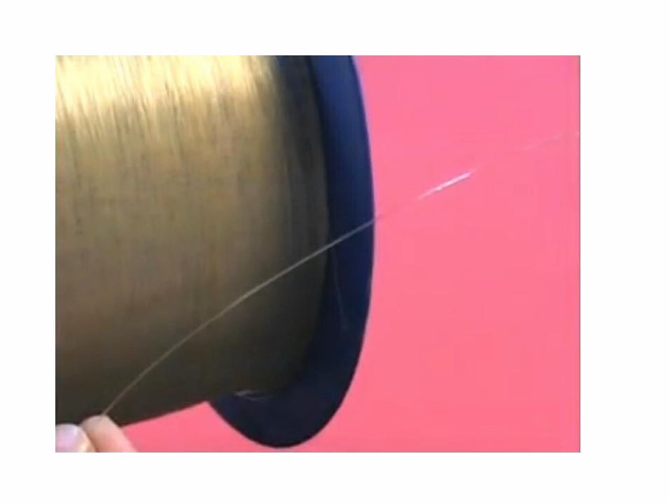
The electromagnetic phenomena can be divided into two categories:Low frequency with high power (electrical machining, power generation, distribution electrical energy…) .High frequency but low power (communications, radar, satellites, optical fiber…)

What are Microwaves?

1 cm

f =10 kHz, = c/f = 3 x 108/ 10 x 103 = 30000 m

Phase delay = )2 or 360) * Physical length/Wavelength

f =10 GHz, = 3 x 108/ 10 x 109 = 3 cm

Electrical length =1 cm/30000 m = 0.33 x 10-6 , Phase delay = 0.00012

RF

Microwave

Electrical length = 0.33 , Phase delay = 118.8

1 360

Electrically long - The phase of a voltage or current changes significantly over the physical extent of the device

Electrical length = Physical length/Wavelength )expressed in )

!!!

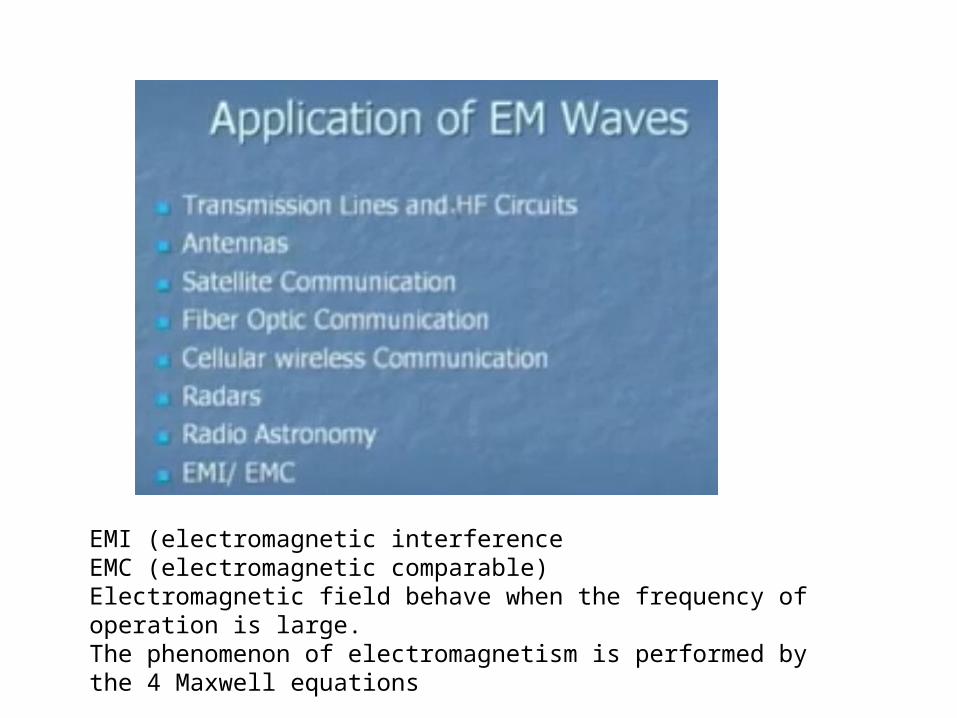
EMI (electromagnetic interferenceEMC (electromagnetic comparable)Electromagnetic field behave when the frequency of operation is large.The phenomenon of electromagnetism is performed by the 4 Maxwell equations

Applications of Microwave Engineering

• The majority of today’s applications of RF and microwave technology are to wire-less networking and communications systems, wireless security systems, radar systems, environmental remote sensing, and medical systems.

• Wireless connectivity promises to provide voice and data access to “anyone, anywhere, at any time.

• Modern wireless telephony is based on the concept of cellular frequency reuse, a technique first proposed by Bell Labs in 1947-1988

• These early systems are usually referred to now as first generation cellular systems, or 1G.

• Microwave oven, Radar, Satellite communication, direct broadcast satellite (DBS) television, personal communication systems (PCSs) etc.

Applications of Microwave Engineering

• Second-generation (2G) cellular systems achieved improved performance by using various digital modulation schemes, with systems such as GSM, CDMA, DAMPS, PCS, and PHS being some of the major standards introduced in the 1990s in the United States, Europe, and Japan.

• These systems can handle digitized voice, as well as some limited data, with data rates typically in the 8 to 14 kbps range.

• In recent years there has been a wide variety of new and modified standards to transition to handheld services that include voice, texting, data networking, positioning, and Internet access.

• These standards are variously known as 2.5G, 3G, 3.5G, 3.75G, and 4G, with current plans to provide data rates up to at least 100 Mbps.

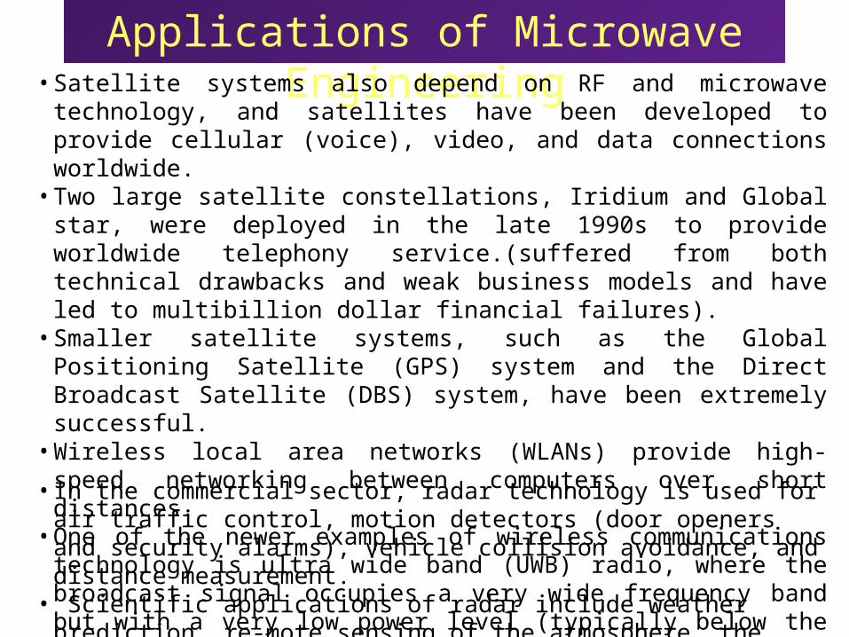
Applications of Microwave Engineering• Satellite systems also depend on RF and microwave technology, and satellites

have been developed to provide cellular (voice), video, and data connections worldwide.

• Two large satellite constellations, Iridium and Global star, were deployed in the late 1990s to provide worldwide telephony service.(suffered from both technical drawbacks and weak business models and have led to multibillion dollar financial failures).

• Smaller satellite systems, such as the Global Positioning Satellite (GPS) system and the Direct Broadcast Satellite (DBS) system, have been extremely successful.

• Wireless local area networks (WLANs) provide high-speed networking between computers over short distances.

• One of the newer examples of wireless communications technology is ultra wide band (UWB) radio, where the broadcast signal occupies a very wide frequency band but with a very low power level (typically below the ambient radio noise level) to avoid interference with other systems.• In the commercial sector, radar technology is used for air traffic control, motion detectors (door openers and security alarms), vehicle collision avoidance, and distance measurement.

• Scientific applications of radar include weather prediction, re-mote sensing of the atmosphere, the oceans, and the ground, as well as medical diagnostics and therapy.

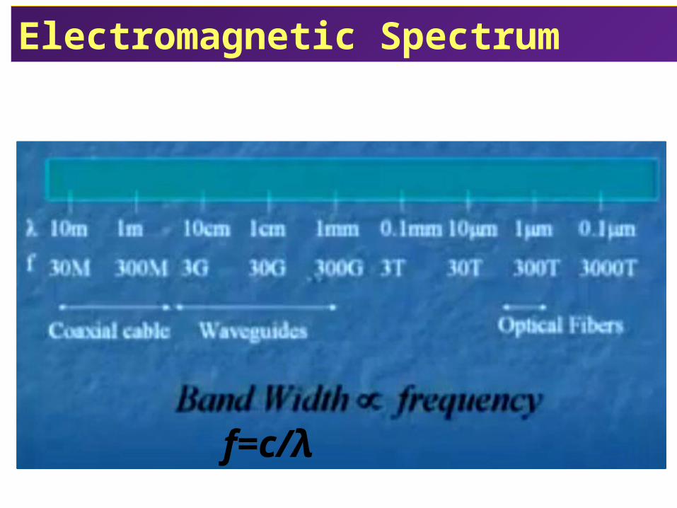
f=c/λ

Electromagnetic Spectrum

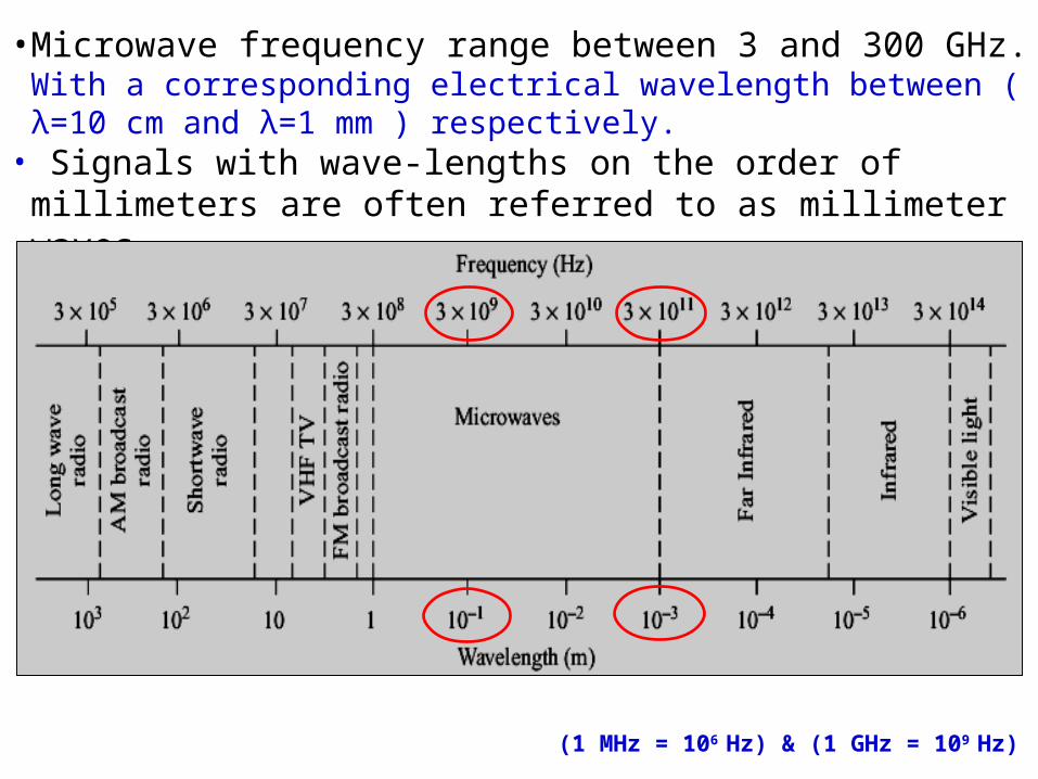
• Microwave frequency range between 3 and 300 GHz. With a corresponding electrical wavelength between ( λ=10 cm and λ=1 mm ) respectively.

• Signals with wave-lengths on the order of millimeters are often referred to as millimeter waves

(1 MHz = 106 Hz) & (1 GHz = 109 Hz)

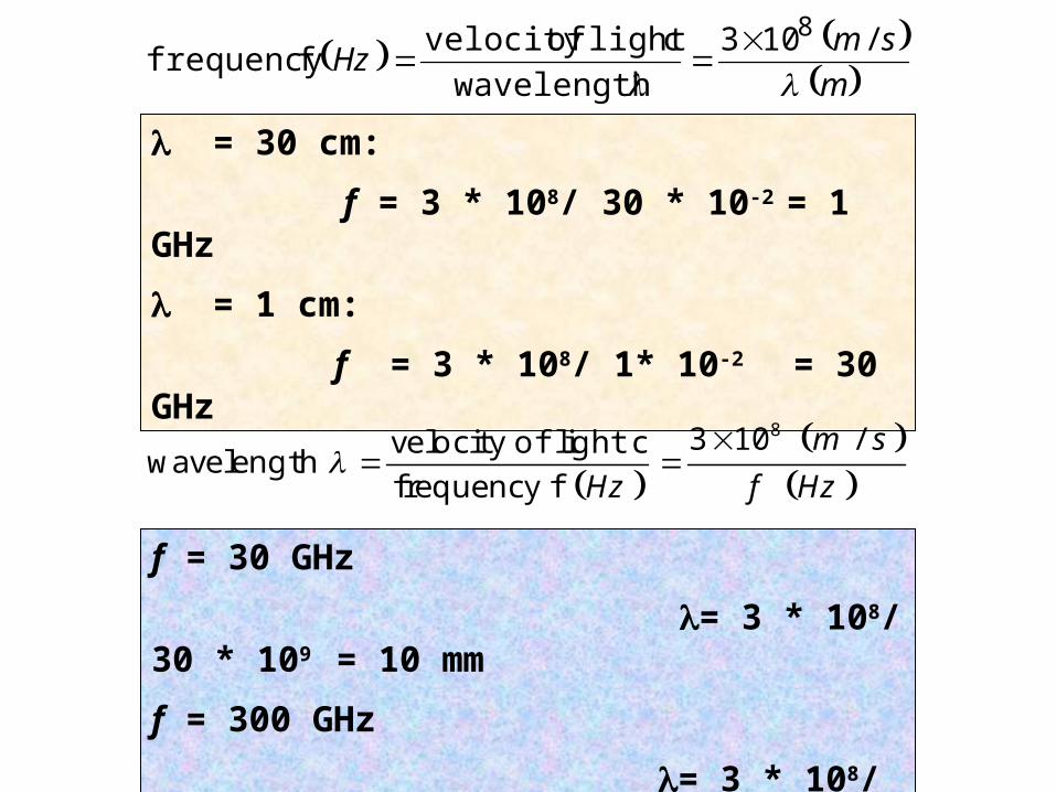
= 30 cm:

f = 3 * 108/ 30 * 10-2 = 1 GHz

= 1 cm:

f = 3 * 108/ 1* 10-2 = 30 GHz

f = 30 GHz

= 3 * 108/ 30 * 109 = 10 mm

f = 300 GHz

= 3 * 108/ 300 * 109 = 1 mm

m

smHz

/ 103

wavelength

clight ofvelocity ffrequency

8

83 10 /velocity of light cwavelength

frequency f

m s

Hz f Hz

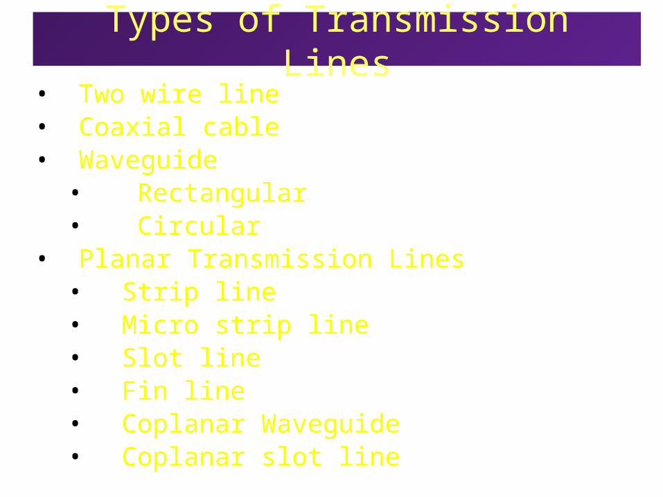
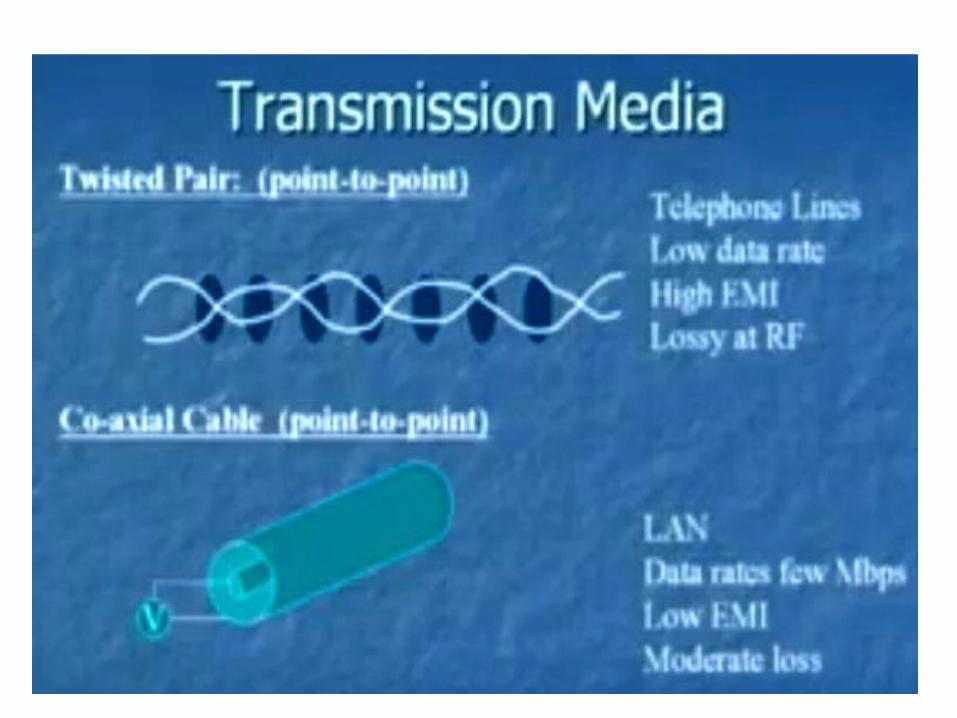
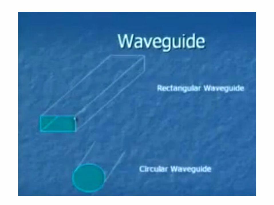
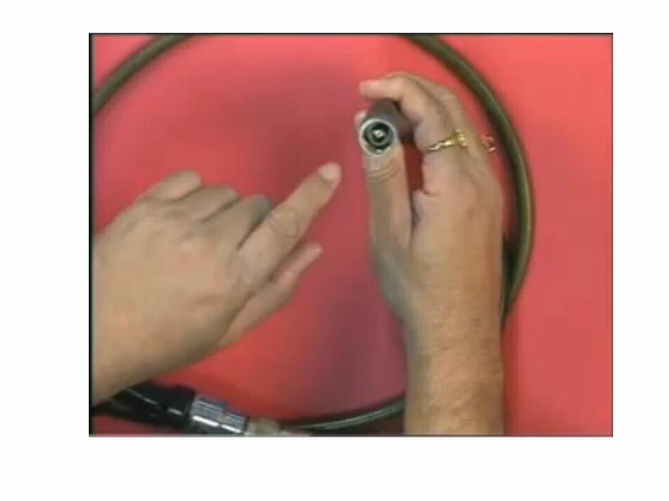
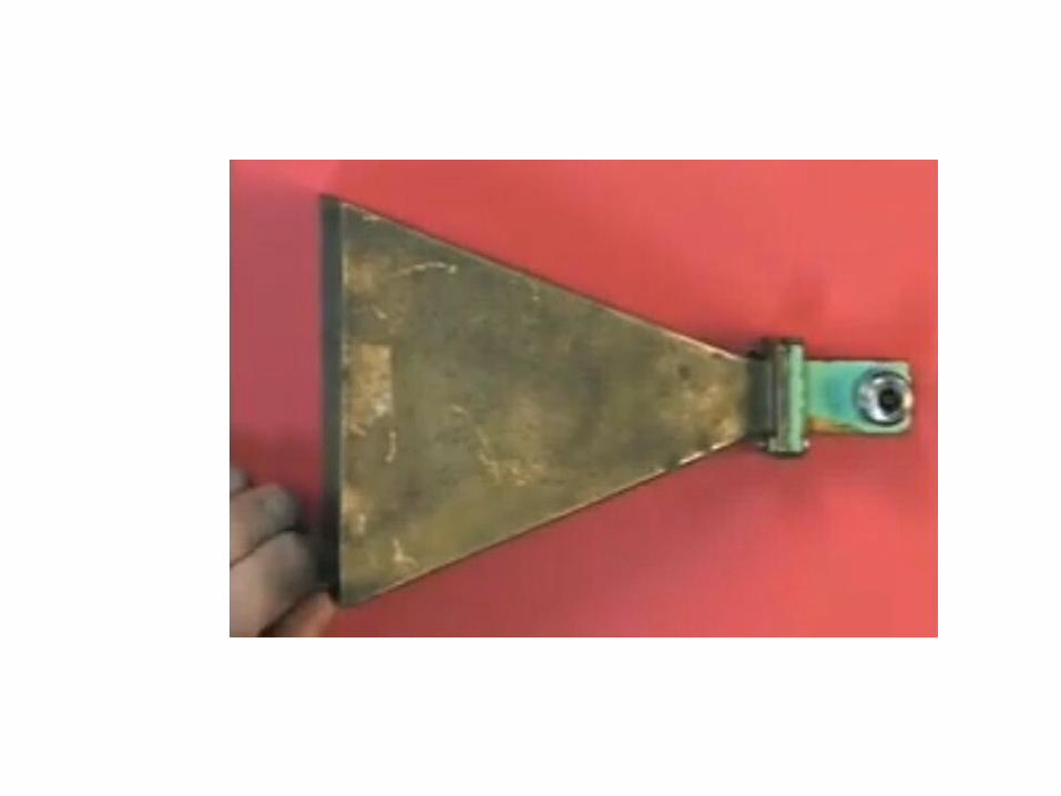
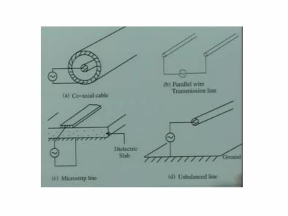
Types of Transmission Lines• Two wire line• Coaxial cable• Waveguide

• Rectangular• Circular

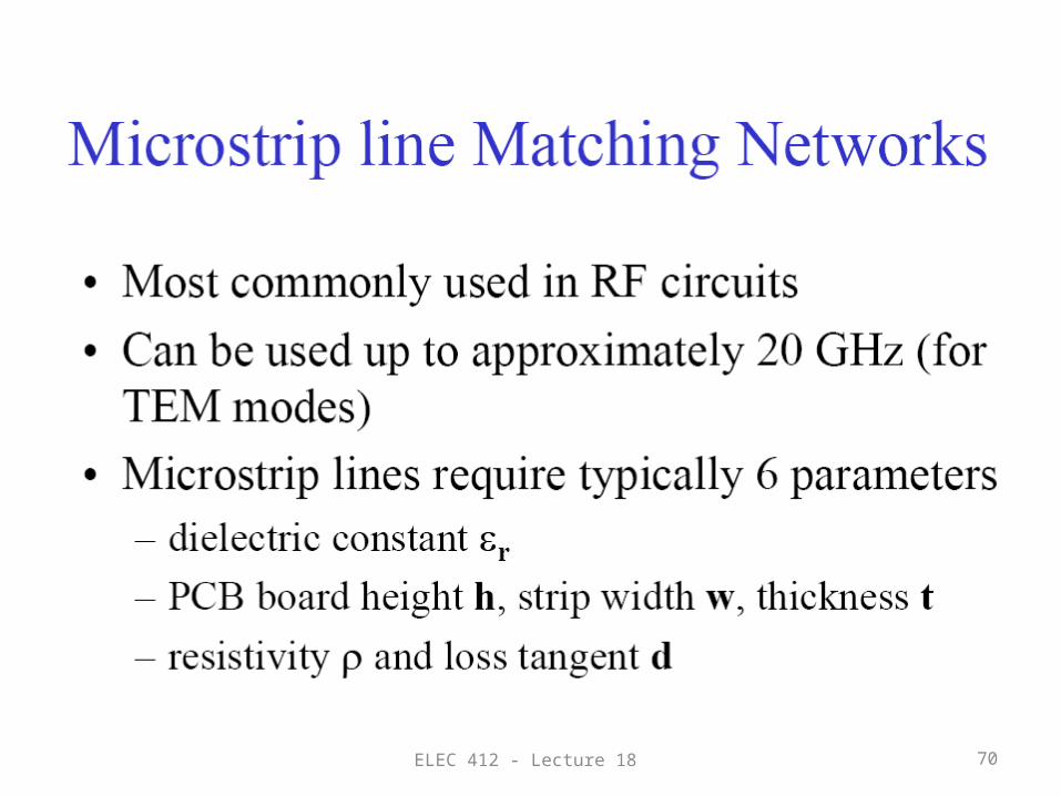
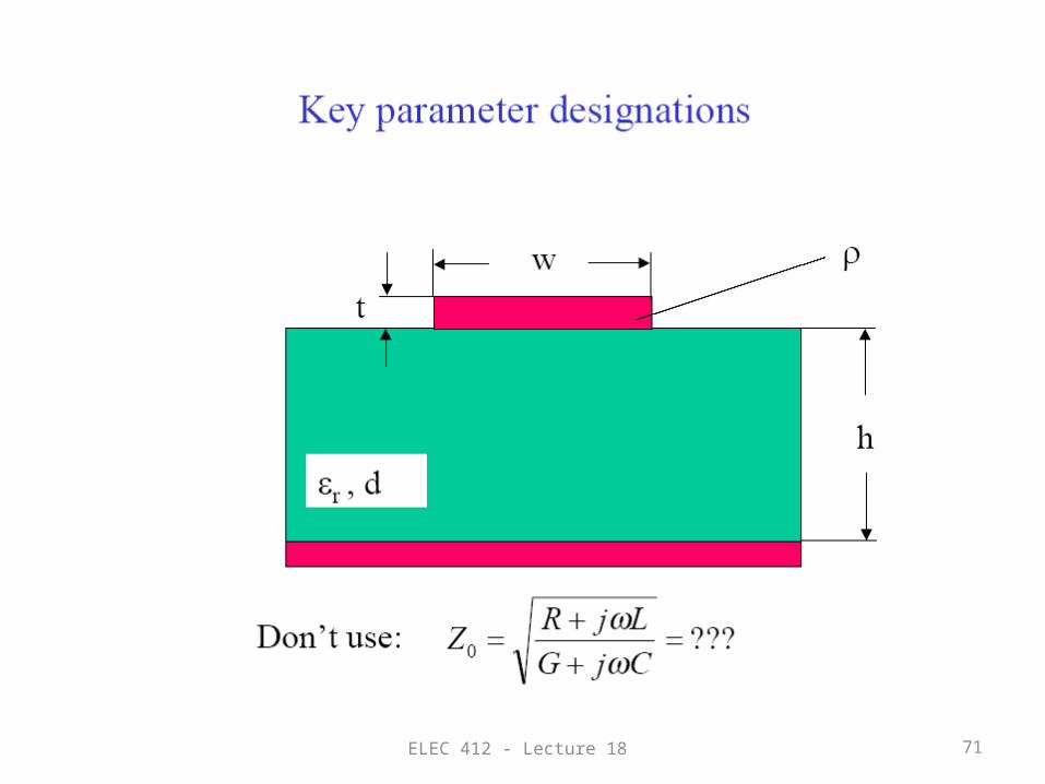
• Planar Transmission Lines• Strip line• Micro strip line• Slot line• Fin line• Coplanar Waveguide• Coplanar slot line

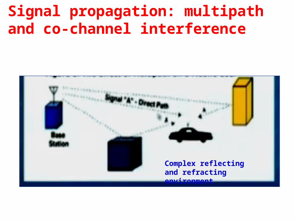
Signal propagation: multipath and co-channel interference

Complex reflecting and refracting environment

• The signal travel as a function of time (time varying electromagnetic fields) with multi path {fading phenomena}.

• Then interference was don which cause destructive (- - -) or constructive (+++) of the signal.

• So a good design of antenna systems will reduce the mobile communication interference.

Signal propagation: multipath and co-channel interference

• The first application of electromagnetic waves is the transmission line (TL).

• (Time varying voltage and current) It is a medium which can transfer power from point to another.

A

A’

B

B’

VQVp

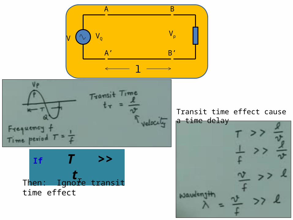
l

V

If T >> tr

Then: Ignore transit time effect

Transit time effect cause a time delay

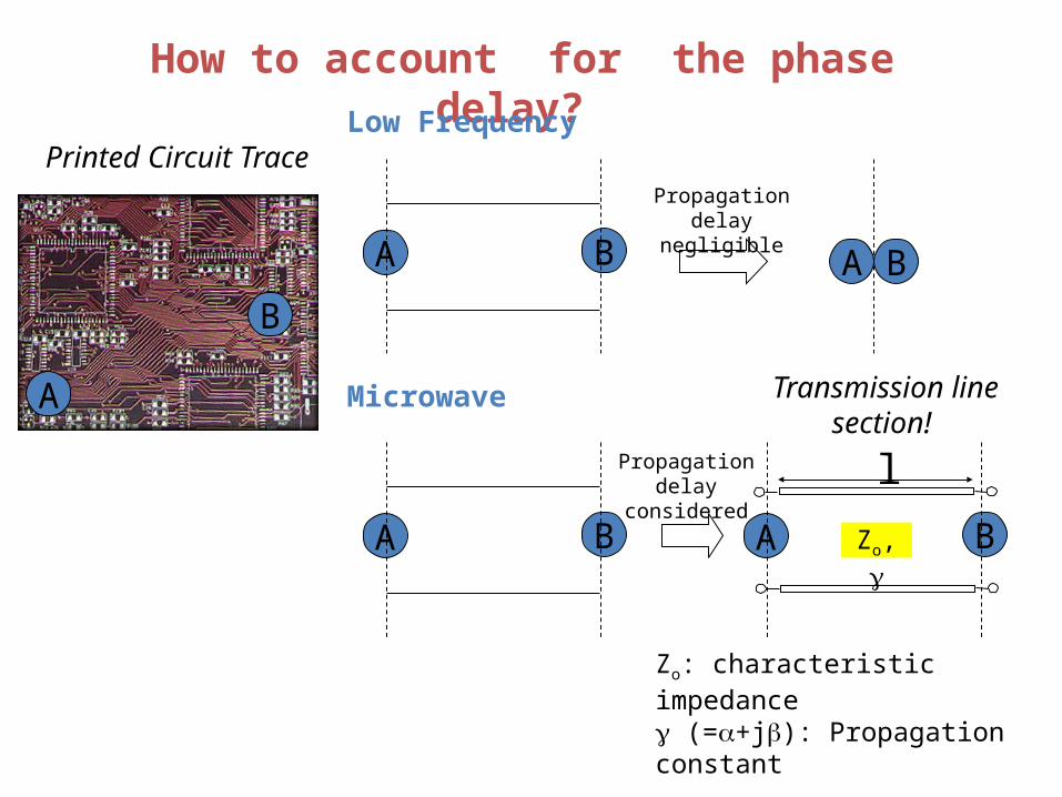
How to account for the phase delay?

A

B

A B A B

Low Frequency

Microwave

A B A B

Propagation delay negligible

Transmission line section!

l

Printed Circuit Trace

Zo: characteristic impedance (=+j): Propagation constant

Zo,

Propagation delay considered

• At much lower frequencies the wavelength is large enough that there is insignificant phase variation across the dimensions of a component.

• Because of the high frequencies (and short wavelengths), standard circuit theory often cannot be used directly to solve microwave network problems.

• Standard circuit theory is an approximation, or special case, of the broader theory of electromagnetic as described by Maxwell’s equations.

• The lumped circuit element approximations of circuit theory may not be valid at high RF and microwave frequencies, where one must work with Maxwell’s equations and their solutions.

• Microwave components often act as distributed elements, where the phase of the voltage or current changes significantly related to device dimensions.

• The solution interested in terminal quantities such as power, impedance, voltage, and current, which can be expressed in terms of circuit theory concepts.

األسبوع الثانى

46

Transmission Line Theory

Transmission Line Theory

47

Any physical structure that guide the electromagnetic wave from place to place is called a Transmission Line (TL).

Introduction

Transmission line theory bridges the gap between field analysis and basic circuit theory, which is important in the analysis of microwave circuits and devices.

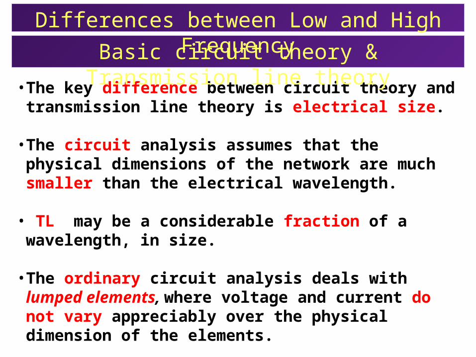
• The key difference between circuit theory and transmission line theory is electrical size.

• The circuit analysis assumes that the physical dimensions of the network are much smaller than the electrical wavelength.

• TL may be a considerable fraction of a wavelength, in size.

• The ordinary circuit analysis deals with lumped elements, where voltage and current do not vary appreciably over the physical dimension of the elements.

• Thus a TL is a distributed parameter network, where voltages and currents can vary in magnitude and phase over its length.

Basic circuit theory & Transmission line theoryDifferences between Low and High Frequency

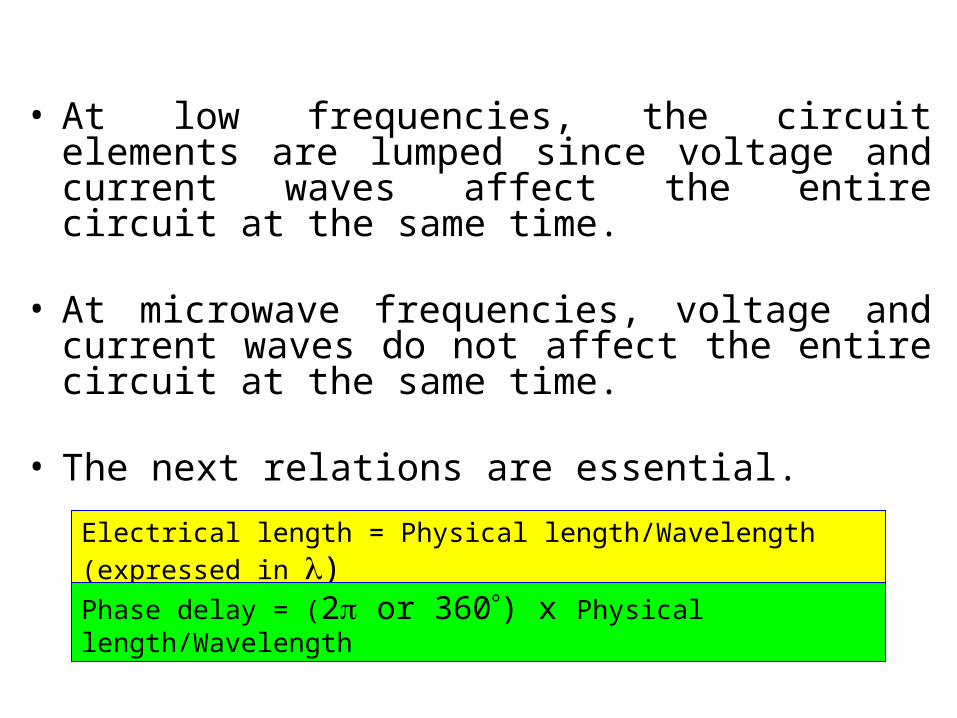
• At low frequencies, the circuit elements are lumped since voltage and current waves affect the entire circuit at the same time.

• At microwave frequencies, voltage and current waves do not affect the entire circuit at the same time.

• The next relations are essential.

Electrical length = Physical length/Wavelength )expressed in )

Phase delay = )2 or 360) x Physical length/Wavelength

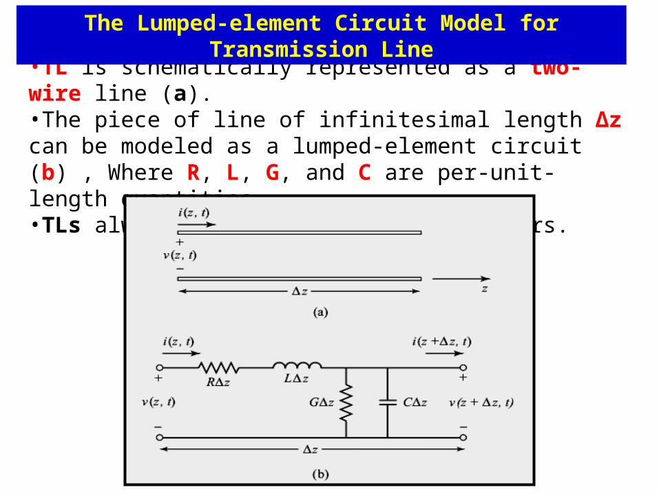
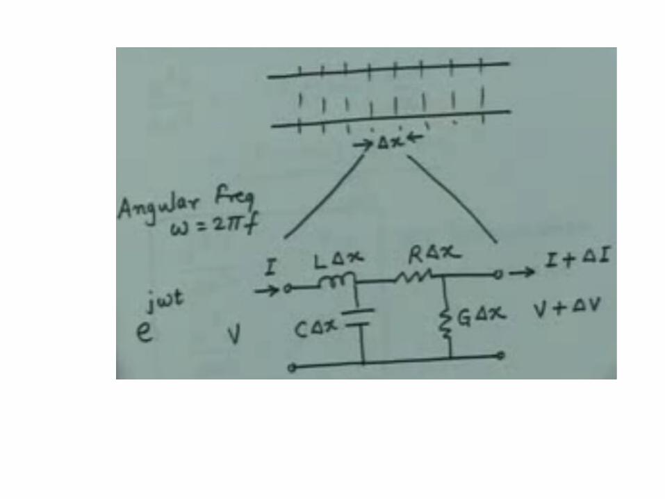
•TL is schematically represented as a two-wire line (a). •The piece of line of infinitesimal length Δz can be modeled as a lumped-element circuit (b) , Where R, L, G, and C are per-unit-length quantities.•TLs always have at least two conductors.

The Lumped-element Circuit Model for Transmission Line

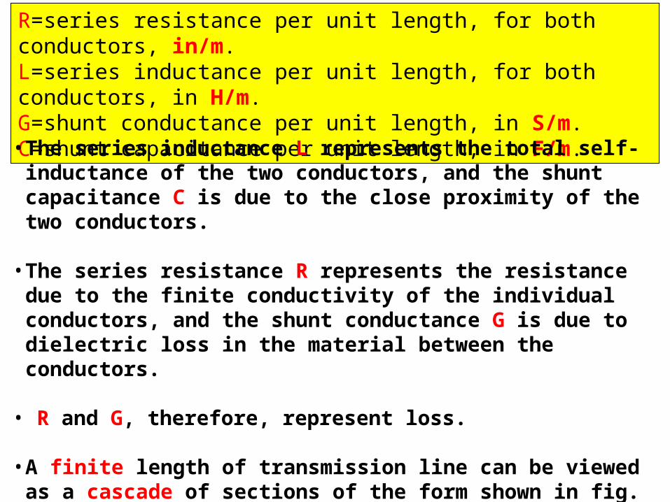
R=series resistance per unit length, for both conductors, in/m.L=series inductance per unit length, for both conductors, in H/m.G=shunt conductance per unit length, in S/m.C=shunt capacitance per unit length, in F/m.

• The series inductance L represents the total self-inductance of the two conductors, and the shunt capacitance C is due to the close proximity of the two conductors.

• The series resistance R represents the resistance due to the finite conductivity of the individual conductors, and the shunt conductance G is due to dielectric loss in the material between the conductors.

• R and G, therefore, represent loss.

• A finite length of transmission line can be viewed as a cascade of sections of the form shown in fig.(b).

• From the circuit of fig.(b), Kirchhoff’s voltage law can be applied as:

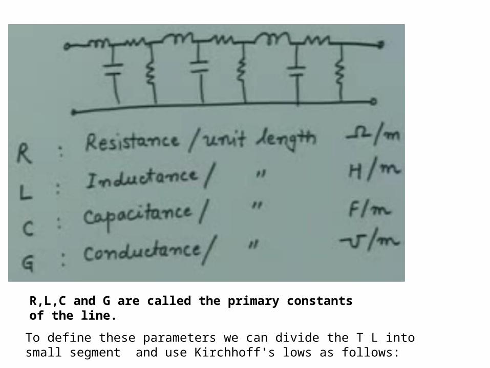
R,L,C and G are called the primary constants of the line.

To define these parameters we can divide the T L into small segment and use Kirchhoff's lows as follows:

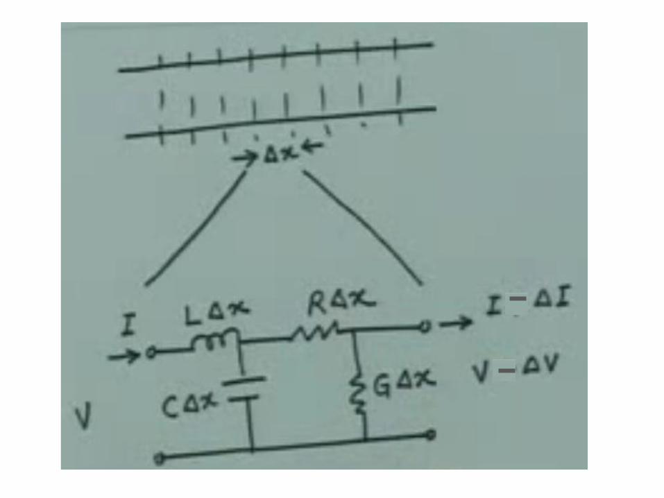
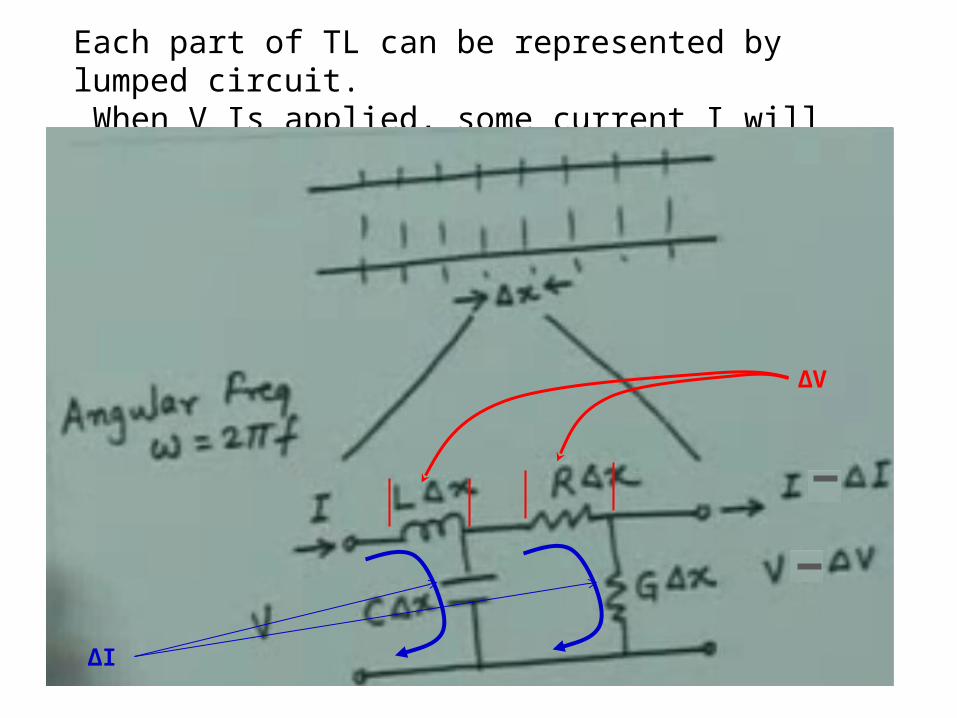
Each part of TL can be represented by lumped circuit. When V Is applied, some current I will flow in the circuit.

ΔI

ΔV

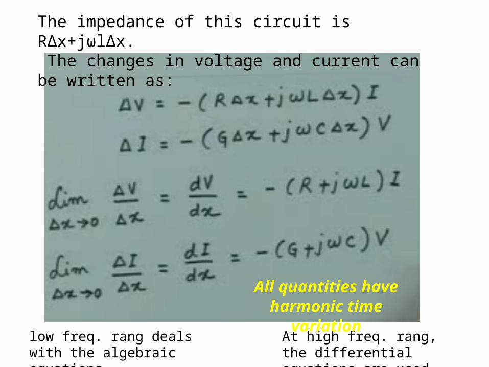
low freq. rang deals with the algebraic equations.

At high freq. rang, the differential equations are used

All quantities have harmonic time variation

The impedance of this circuit is RΔx+jωlΔx. The changes in voltage and current can be written as:

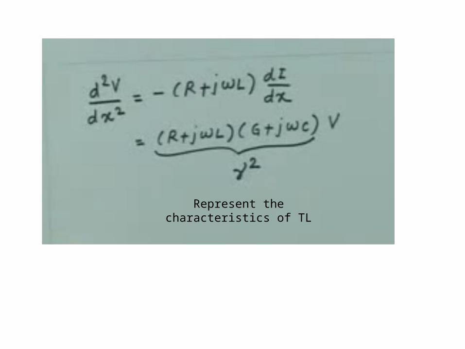
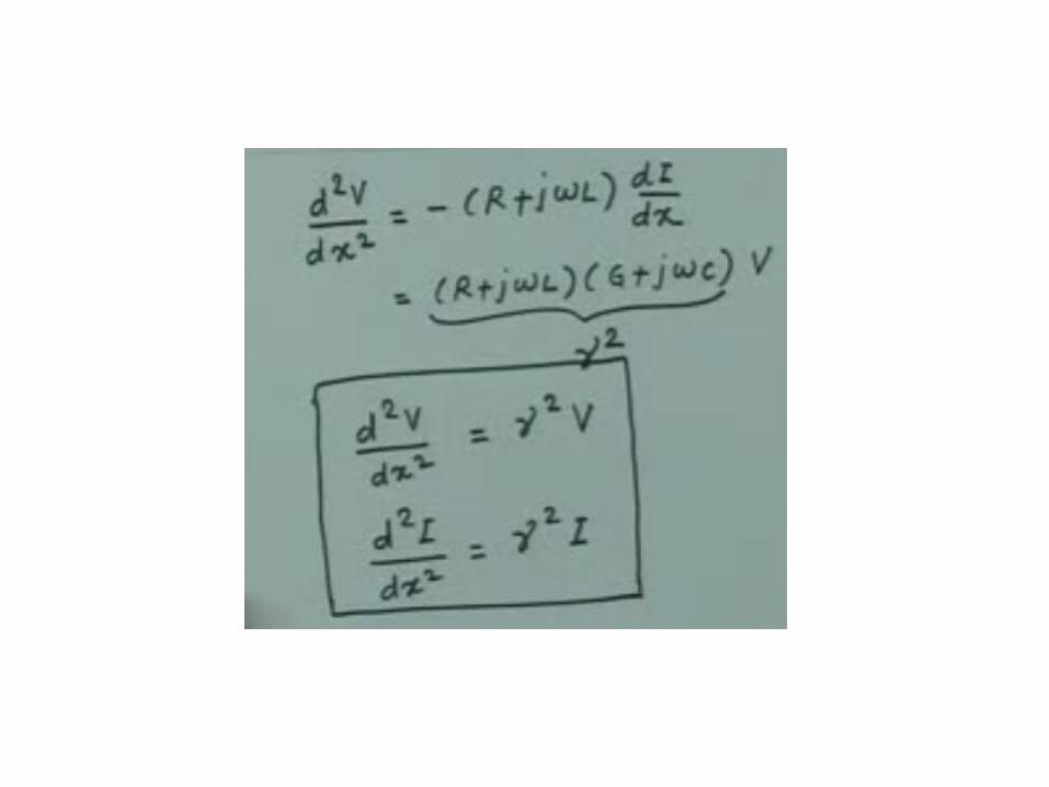
Represent the characteristics of TL

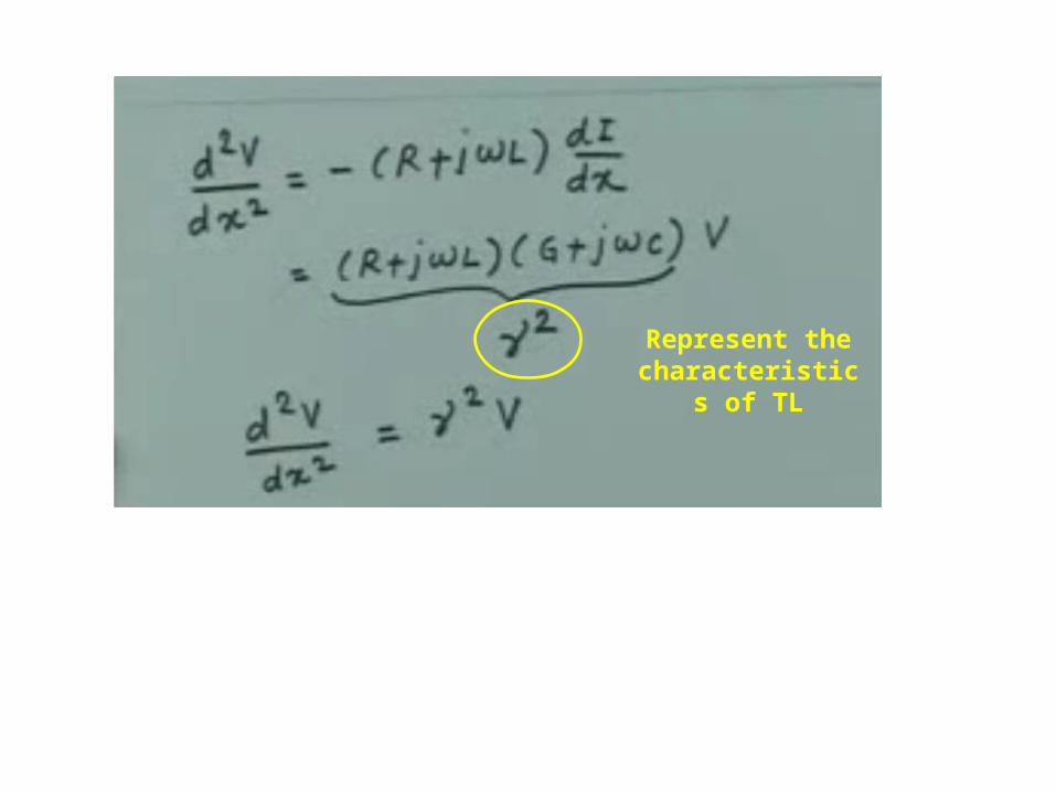
Represent the characteristics of TL

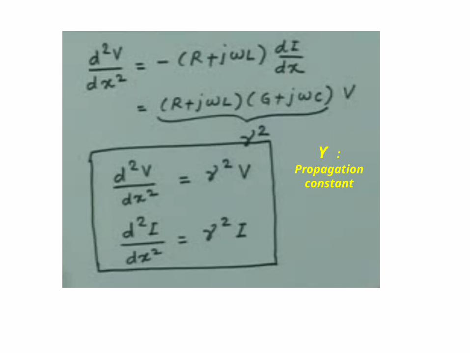
Ƴ : Propagation constant

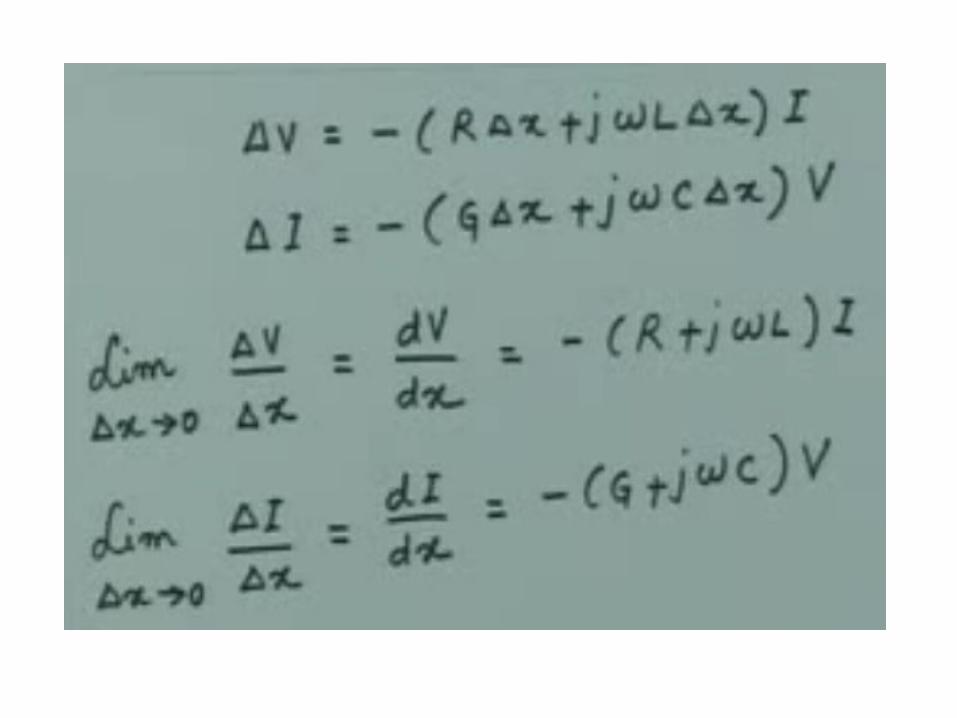
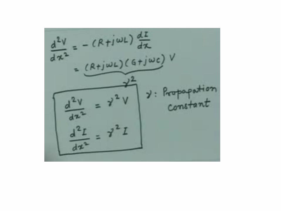
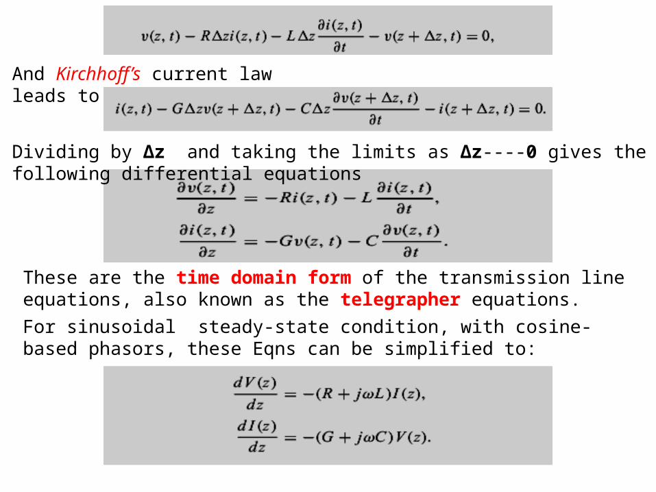
These are the time domain form of the transmission line equations, also known as the telegrapher equations.

Dividing by Δz and taking the limits as Δz----0 gives the following differential equations

For sinusoidal steady-state condition, with cosine-based phasors, these Eqns can be simplified to:

And Kirchhoff’s current law leads to:

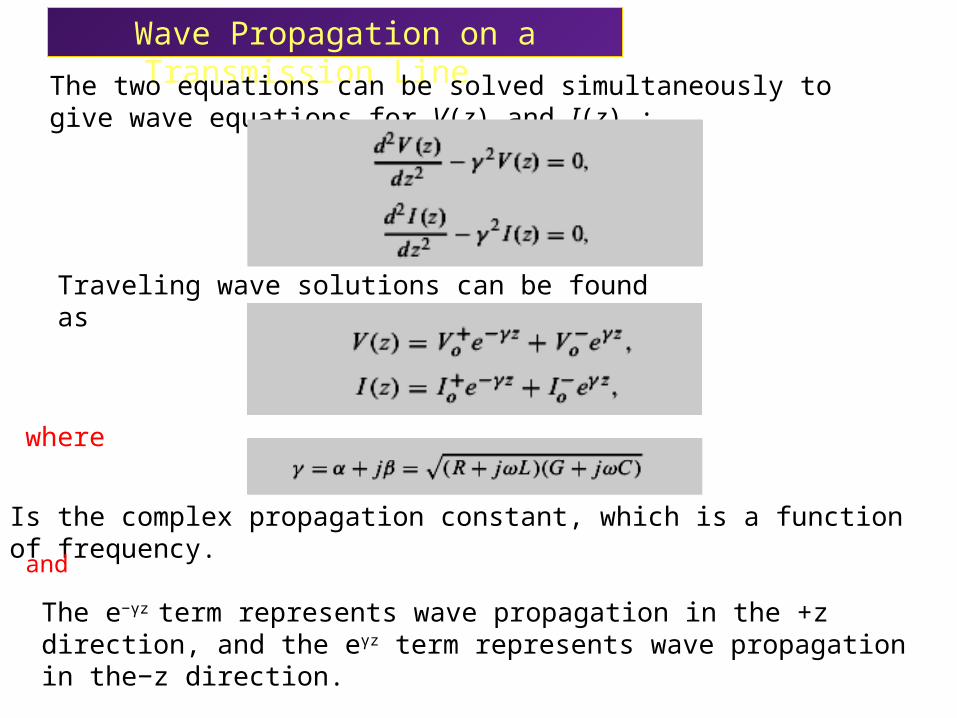
Wave Propagation on a Transmission Line

The two equations can be solved simultaneously to give wave equations for V(z) and I(z) :

Is the complex propagation constant, which is a function of frequency.

where

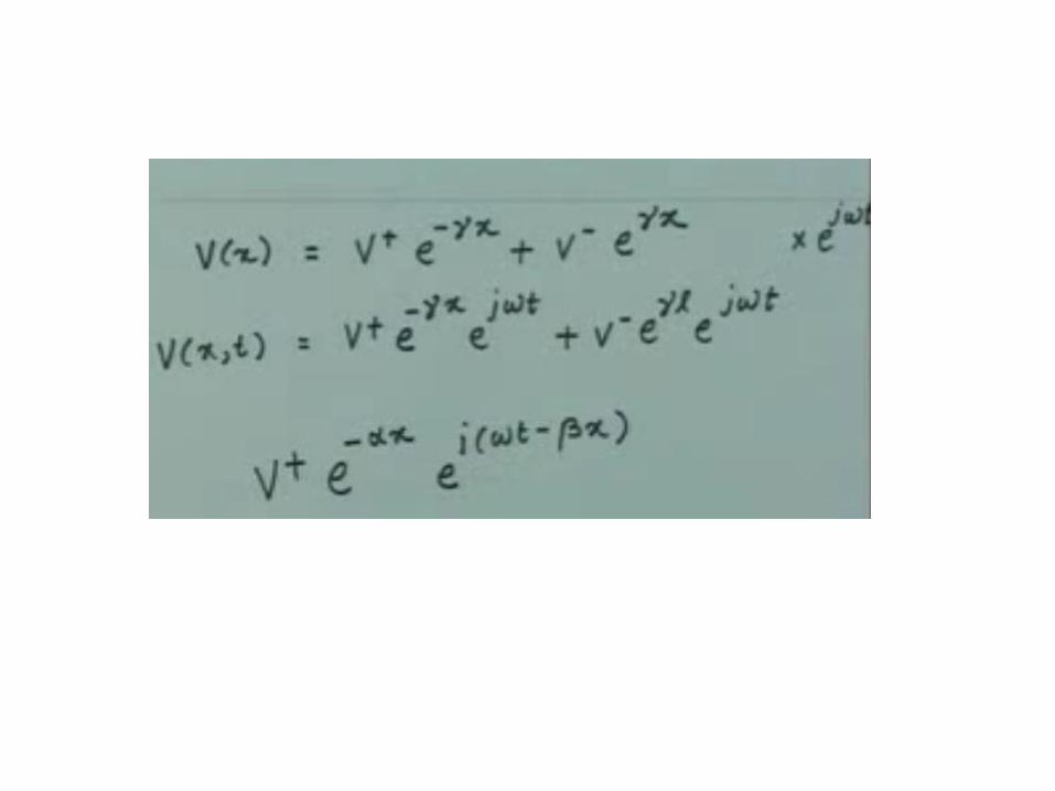
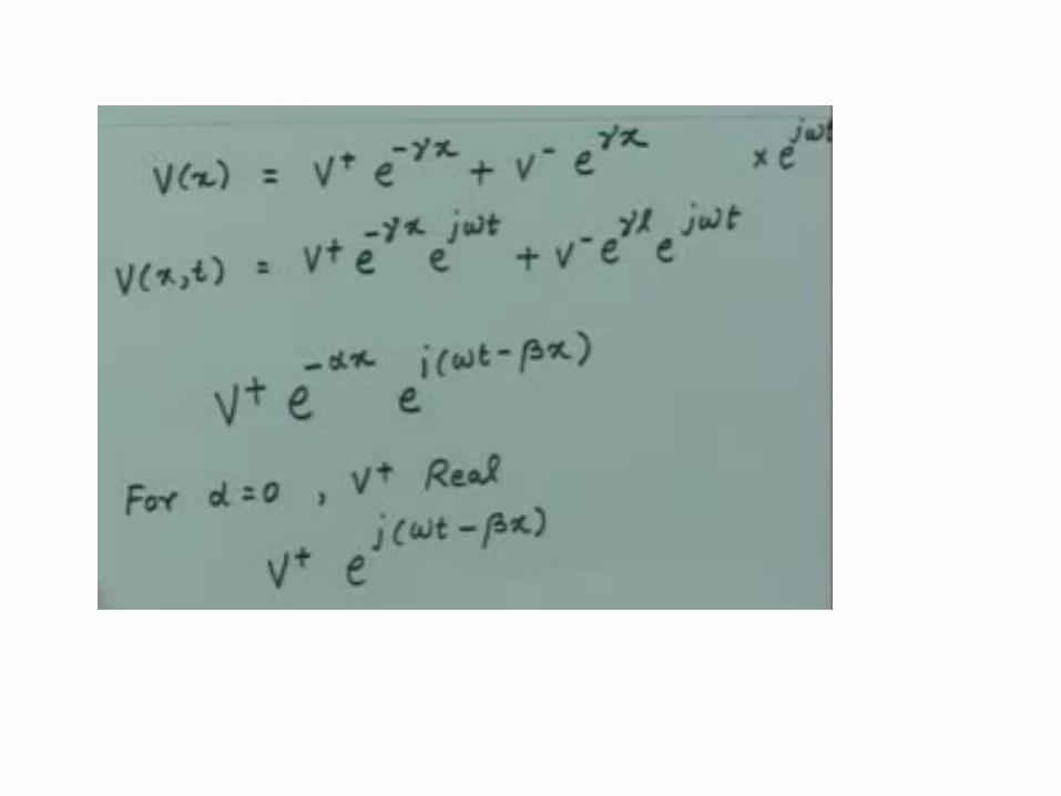
Traveling wave solutions can be found as

and

The e−γz term represents wave propagation in the +z direction, and the eγz term represents wave propagation in the−z direction.

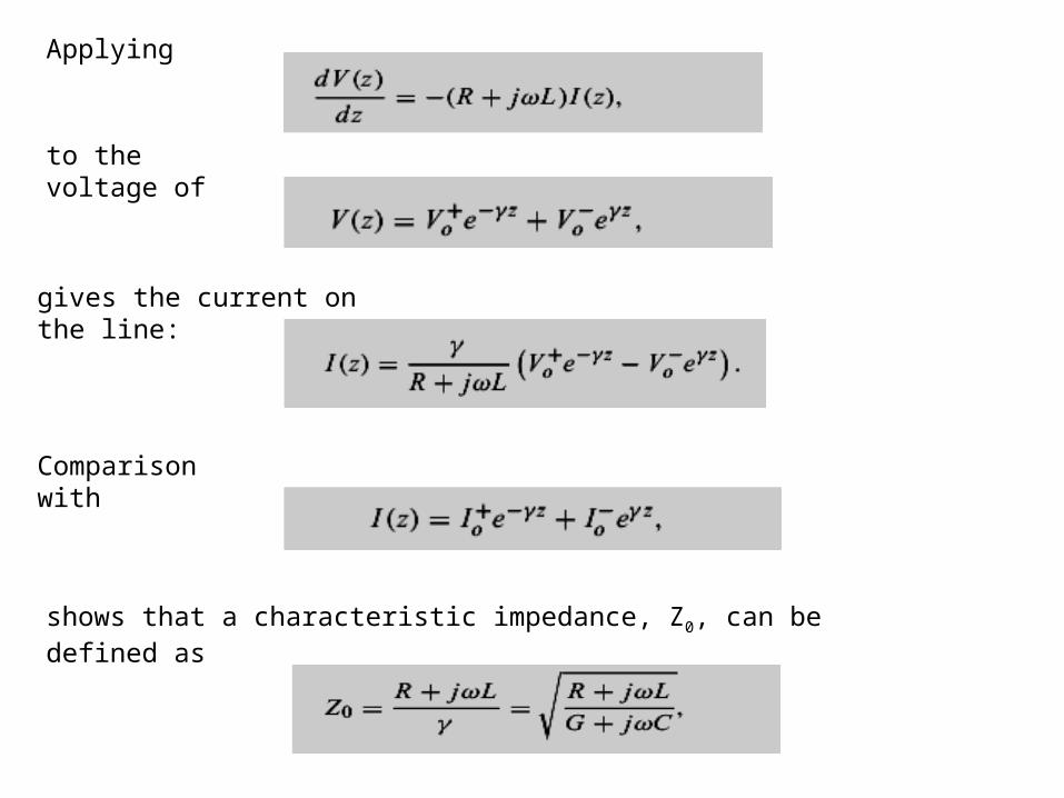
Applying

Comparison with

to the voltage of

gives the current on the line:

shows that a characteristic impedance, Z0, can be defined as

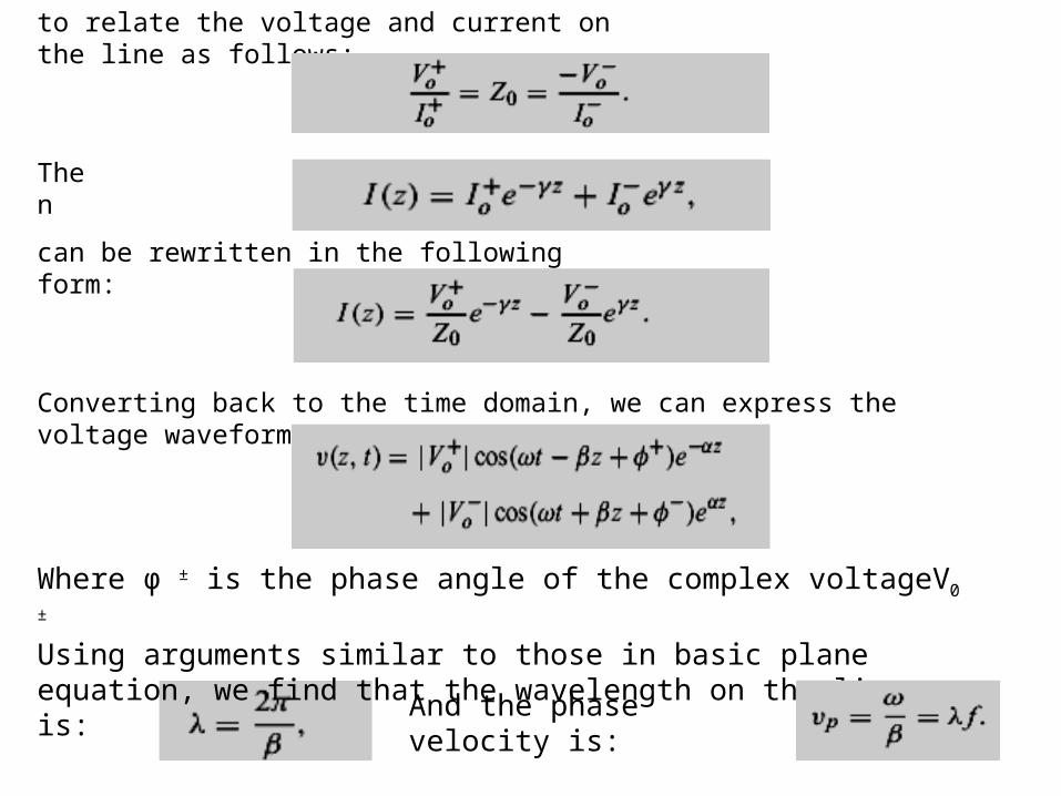
to relate the voltage and current on the line as follows:

Then

Converting back to the time domain, we can express the voltage waveform as

Where φ ± is the phase angle of the complex voltageV0 ±

Using arguments similar to those in basic plane equation, we find that the wavelength on the line is:

can be rewritten in the following form:

And the phase velocity is:

ELEC 412 - Lecture 18 70




Documents

الفصل الدراسى السابع S-7 هندسة ميكروموجية Microwave Engineering 1