沈致远

^2^

^

( ( ))( , ( ))

| ( ) |

Y f XL Y f X

Y f X

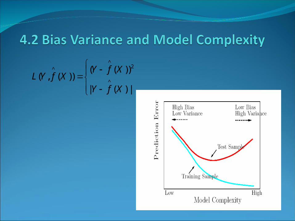
Test error(generalization error): the expected prediction error over an independent test sample

Training error: the average loss over the training sample.

^

[ ( , ( ))]Err E L Y f X

_____ ^

1

1( , ( ))

N

ii

err L y f XN

It is important to note that there are in fact two separate goals that we might have in mind:

Model Selection: estimating the performance of different models in order to choose the (approximate) best one.

Model Assessment: having chosen a final model, estimating its prediction error(generalization error) on new data.

If we are in a data-rich situation, the best approach for both problem is to randomly divide the dataset into three parts: a training set, a validation set, and a test set.The training set: fit the modelThe validation set: estimate prediction error for model selection.The test set: assessment of the generalization error of the final chosen model.

Train Validation Test

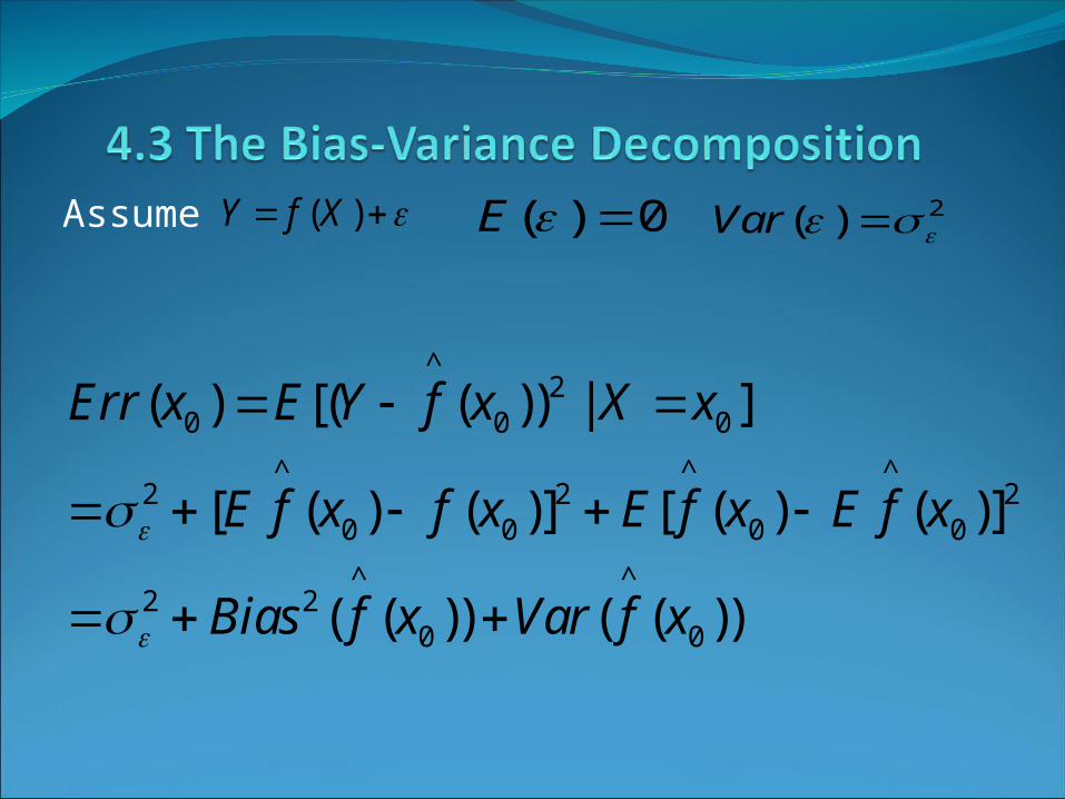
Assume ( )Y f X ( ) 0E 2( )Var

^2

0 0 0

^ ^ ^2 2 2

0 0 0 0

^ ^2 2

0 0

( ) [( ( )) | ]

[ ( ) ( )] [ ( ) ( )]

( ( )) ( ( ))

Err x E Y f x X x

E f x f x E f x E f x

Bias f x Var f x

For k-nearest –neighbor regression fit

^2

0 0 0

2 2 20

1

( ) [( ( )) | ]

1[ ( ) ( )] /

k

k

ll

Err x E Y f x X x

f x f x kk

For a linear model fit,^

20 0 0

^2 2 2 2

0 0 0

( ) [( ( )) | ]

[ ( ) ( )] || ( ) ||

p

p

Err x E Y f x X x

E f x f x h x

^2 2 2

1 1

1 1( ) [ ( ) ( )]

N N

i i ii i

pErr x E f x f x

N N N

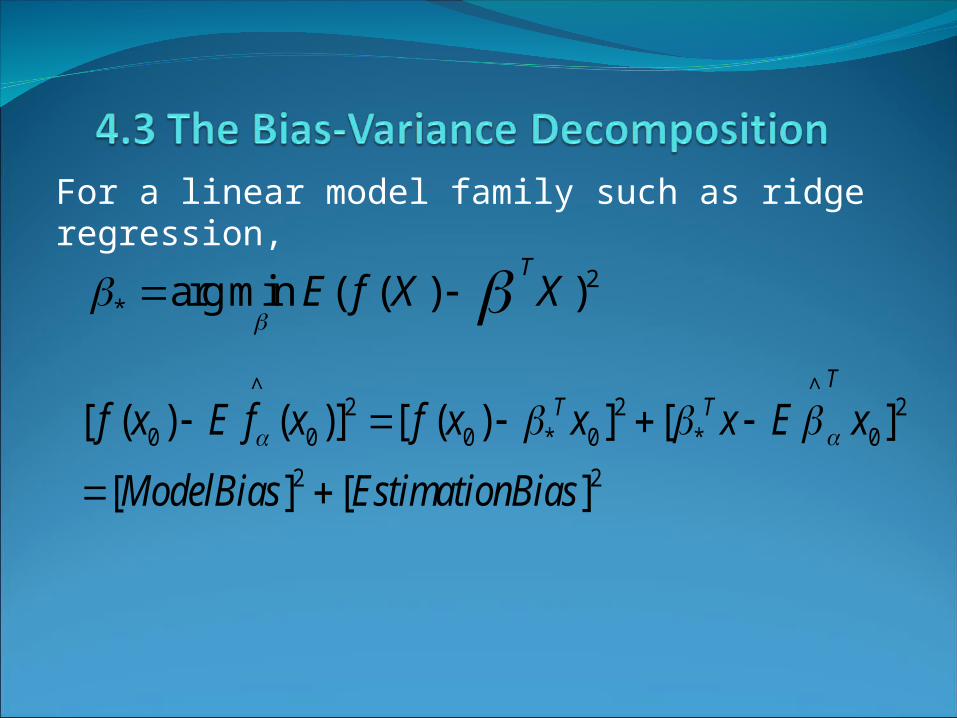
For a linear model family such as ridge regression,

2* argmin ( ( ) )

TE f X X

^ ^2 2 2

0 0 0 * 0 * 0

2 2

[ ( ) ( )] [ ( ) ] [ ]

[ ] [ ]

TT Tf x E f x f x x x E x

ModelBias EstimationBias

Typically, the training error rate

will be less than the true rate because the same data is being used to fit the model and assess its error. A fitting method typically adapts to the training data and hence the apparent or training error will be an overly optimistic estimate of the generalization error.

____ ^

1

1( , ( ))

N

i ii

err L y f xN

^

[ ( , ( ))]Err E L Y f X

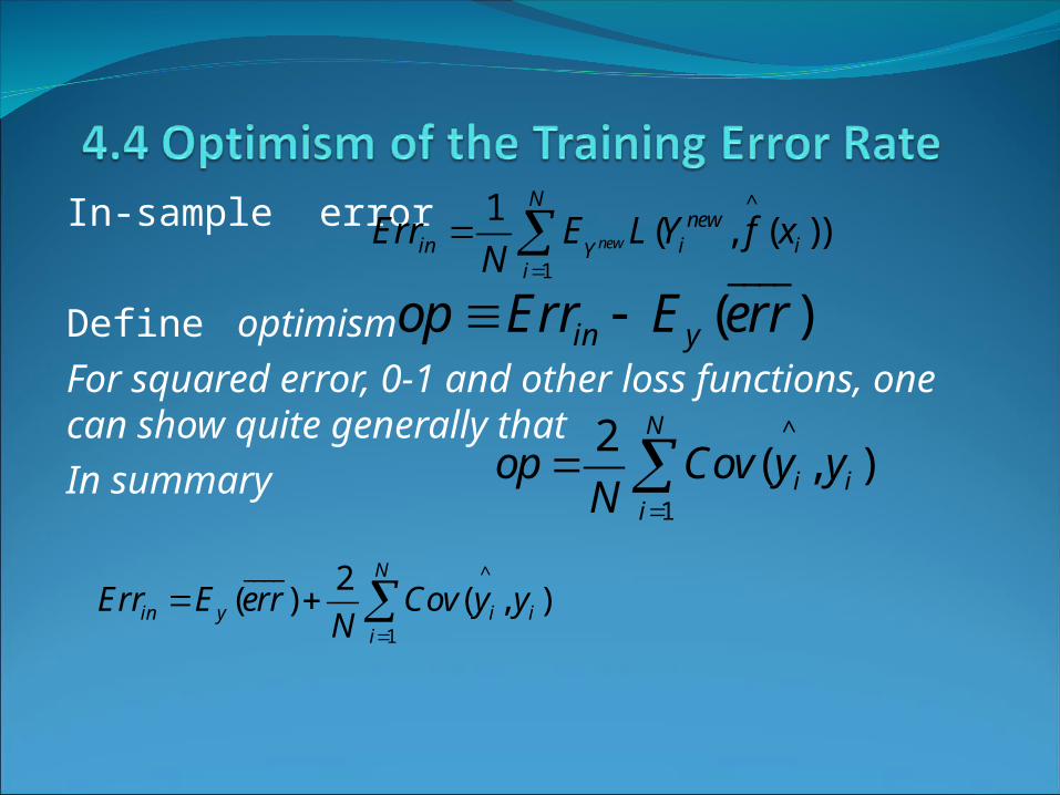
In-sample error

Define optimismFor squared error, 0-1 and other loss functions, one can show quite generally thatIn summary

^

1

1( , ( ))new

Nnew

in i iYi

Err E L Y f xN

____

( )in yop Err E err

^

1

2( , )

N

i ii

op Cov y yN

____ ^

1

2( ) ( , )

N

in y i ii

Err E err Cov y yN

If is obtained by a linear fit with d inputs or basis functions, for the additive error model

So

^

iy( )Y f X

^2

1

( , )N

i ii

Cov y y d

____2( ) 2in y

dErr E err

N

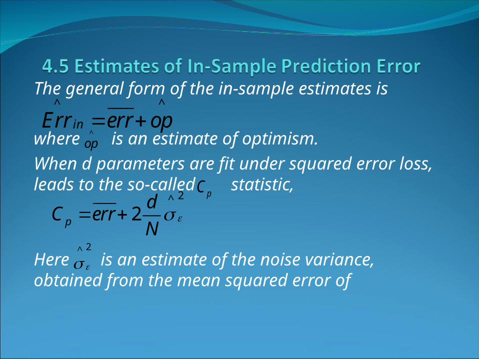
The general form of the in-sample estimates is

where is an estimate of optimism.When d parameters are fit under squared error loss, leads to the so-called statistic,

Here is an estimate of the noise variance, obtained from the mean squared error of

____^ ^

inErr err op ^

op

pC2____ ^

2p

dC err

N

2^

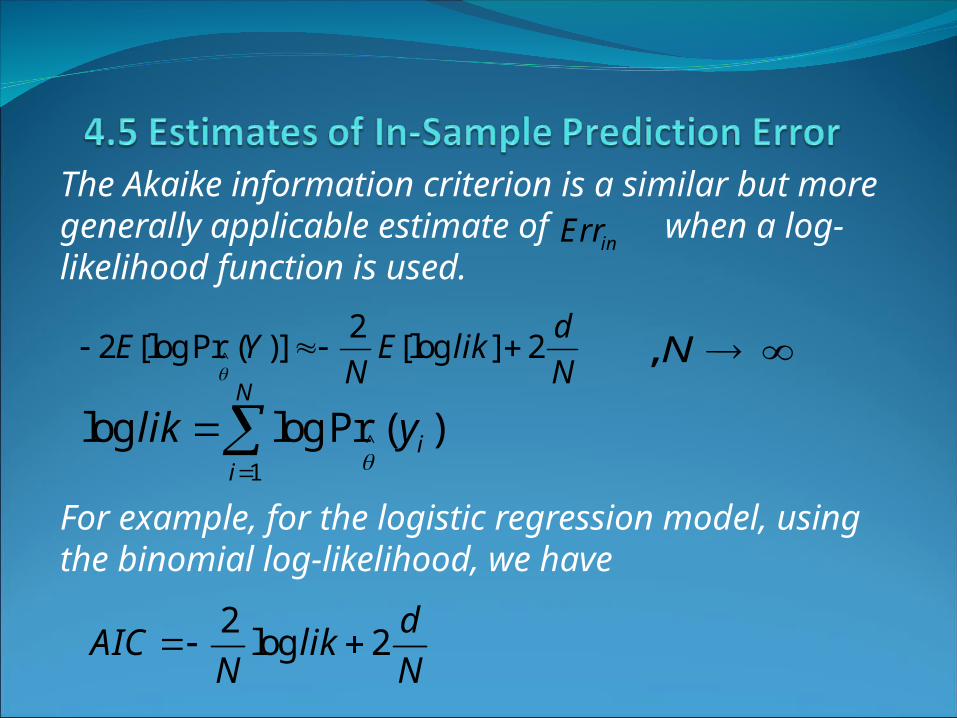
The Akaike information criterion is a similar but more generally applicable estimate of when a log-likelihood function is used.

For example, for the logistic regression model, using the binomial log-likelihood, we have

inErr

^

22 [log Pr ( )] [log ] 2

dE Y E lik

N N ,N

^

1

log log Pr ( )N

ii

lik y

2log 2

dAIC lik

N N

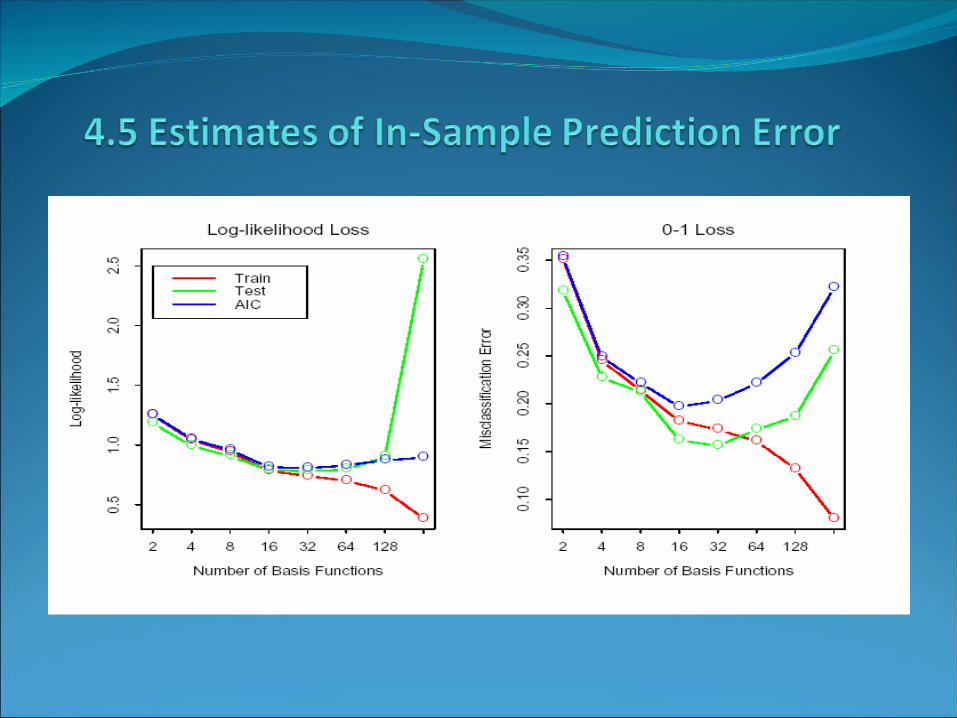
Given a set of models indexed by a tuning parameters denote by and the training error and number of parameters for each model. Then for this set of models we define

The function AIC provides an estimate of the test error curve, and we find the tuning parameter that minimizes it. Our final chosen model is

2____ ^( )( ) ( ) 2

dAIC err

N

( )xf

____

( )err ( )d

^

^ ( )xf

The effective number of parameters is defined as

^

y Sy

( ) ( )d S trace S

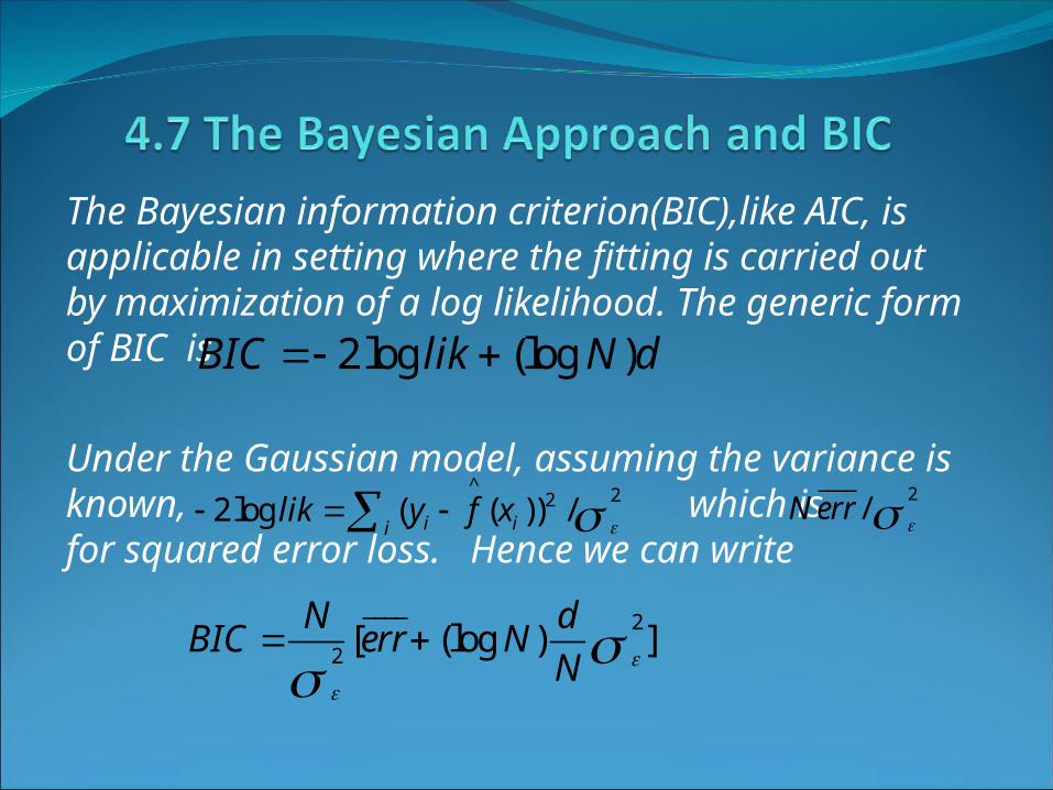
The Bayesian information criterion(BIC),like AIC, is applicable in setting where the fitting is carried out by maximization of a log likelihood. The generic form of BIC is

Under the Gaussian model, assuming the variance is known, which is for squared error loss. Hence we can write

2log (log )BIC lik N d

^ 222log ( ( )) /i iilik y f x

____2

2 [ (log ) ]N d

BIC err NN

____2

/N err

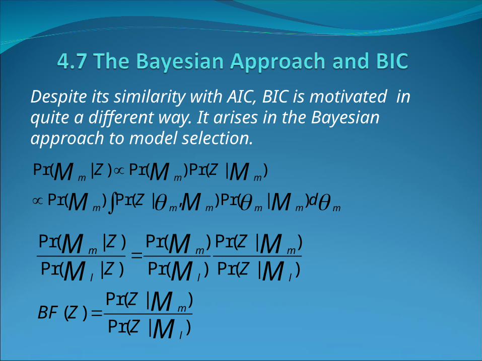
Despite its similarity with AIC, BIC is motivated in quite a different way. It arises in the Bayesian approach to model selection.

Pr( | ) Pr( ) Pr( | )

Pr( ) Pr( | , ) Pr( | )

m m m

m m mm m m

Z Z

Z d

M M MM M M

Pr( | ) Pr( ) Pr( | )

Pr( | ) Pr( ) Pr( | )

Pr( | )( )

Pr( | )

m m m

l l l

m

l

Z Z

Z Z

ZBF Z

Z

M M MM M M

MM

Loss function:

The posterior probability of each model

^

log Pr( | ) log Pr( | , ) log (1)2m

mm m

dZ Z N OM M

^

2log Pr( | , )m mZ M

mM1

2

1

2

1

m

l

BIC

M BIC

l

e

e

Loss function:

The posterior probability of each model

^

log Pr( | ) log Pr( | , ) log (1)2m

mm m

dZ Z N OM M

^

2log Pr( | , )m mZ M

mM1

2

1

2

1

m

l

BIC

M BIC

l

e

e

The minimum description length(MDL) approach gives a selection criterion formally identical to the BIC approach, but is motivated from an optimal coding viewpoint.

Message

Z1 Z2 Z3 Z4

Code 0 10 110 111

How we decide which to use? It depends on how often we will be sending each of the messages. If, for example, we will be sending Z1 most often , it makes sense to use the shortest code 0 for Z1. Using this kind of strategy-shorter codes for more frequent messages-the average message length will be shorter.In general, if messages are sent with probabilitiesa famous theorem due to Shannon says we should use code lengths and the average message length satisfies

Pr( )iz

2log Pr( )iizl

2( ) Pr( ) log (Pr( ))i iE length z z

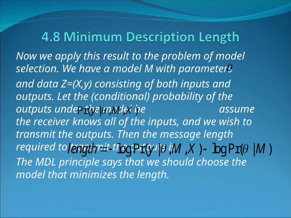
Now we apply this result to the problem of model selection. We have a model M with parametersand data Z=(X,y) consisting of both inputs and outputs. Let the (conditional) probability of the outputs under the model be assume the receiver knows all of the inputs, and we wish to transmit the outputs. Then the message length required to transmit the outputs isThe MDL principle says that we should choose the model that minimizes the length.

Pr( | , , )y M X

log Pr( | , , ) log Pr( | )length y M X M

K-fold cross-validation uses part of the available data to fit the model and a different part to test it. We split the data into K roughly equal-sized parts; for example K=5,

Let be an indexing function that indicates the partition to which observation i is allocated by the randomization. Denote by the fitted function, computed with the kth part of the data removed. Then the cross-validation estimate of prediction error is

Train

Train Test Train Train

:{1, } {1, }N K ……， ……，

^

( )kf x

^( )

1

1( , ( ))

Ni

i ii

CV L y f xN

Generalized cross-validation

^^

2 2

1 1

( )1 1[ ( )] [ ]

1

N Ni i i

i ii i ii

y f xy f x

N N S

^

2

1

( )1[ ]1 ( ) /

Ni i

i

y f xGCV

N trace S N

In the figure, S(Z) is any quantity computed from the data Z, for example, the prediction at some input point. From the bootstrap sampling we can estimate any aspect of the distribution of S(Z), for example its variance,^

* * 2

1

1[ ( )] ( ( ) )

1

Bb

b

Var S Z S Z SB

^^*

1 1

1 1( , ( ))

B Nb

boot i ib i

Err L y f xB N

The leave-one-out bootstrap estimate of prediction error is define by

The “.632 estimator” is designed to alleviate this bias.

^ ^(1) *

1

1 1( , ( ))

| | i

Nb

i iii b C

Err L y f xN C

^^(.632) ____(1).368 .632Err err Err

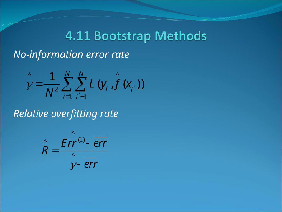
No-information error rate

Relative overfitting rate

'

'

^ ^

21 1

1( , ( ))

N N

i ii i

L y f xN

^ ____(1)^

____^

Err errR

err

We define “.632+” estimator by

^^(.632 ) ____^ ^(1)(1 )Err err Err

^

^

.632

1 .368R

Thanks a lot!